Evolutionary tree reconstruction (Chapter 10)

Evolutionary tree reconstruction(Chapter 10)

Early Evolutionary Studies• Anatomical features were the dominant criteria

used to derive evolutionary relationships between species since Darwin till early 1960s

• The evolutionary relationships derived from these relatively subjective observations were often inconclusive. Some of them were later proved incorrect

Evolution and DNA Analysis: the Giant Panda Riddle

• For roughly 100 years scientists were unable to figure out which family the giant panda belongs to

• Giant pandas look like bears but have features that are unusual for bears and typical for raccoons, e.g., they do not hibernate

• In 1985, Steven O’Brien and colleagues solved the giant panda classification problem using DNA sequences and algorithms

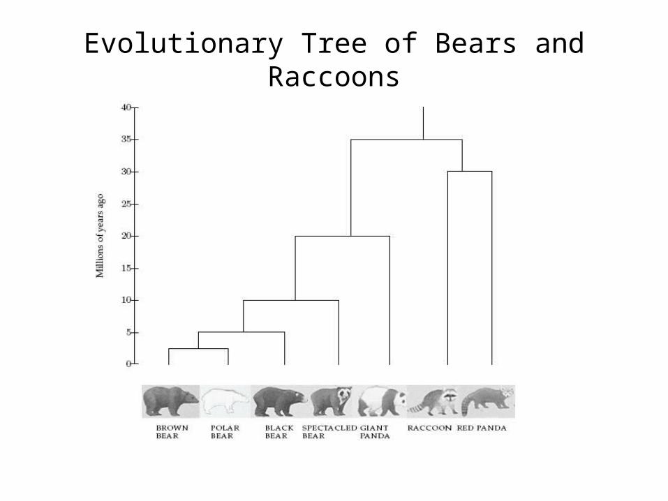
Evolutionary Tree of Bears and Raccoons

Out of Africa Hypothesis

• DNA-based reconstruction of the human evolutionary tree led to the Out of Africa Hypothesis that claims our most ancient ancestor lived in Africa roughly 200,000 years ago

mtDNA analysis supports “Out of Africa” Hypothesis

• African origin of humans inferred from:– African population was the most diverse

(sub-populations had more time to

diverge)– The evolutionary tree separated one

group of Africans from a group containing all five populations.

– Tree was rooted on branch between groups of greatest difference.

Evolutionary tree

• A tree with leaves = species, and edge lengths representing evolutionary time

• Internal nodes also species: the ancestral species

• Also called “phylogenetic tree”

• How to construct such trees from data?

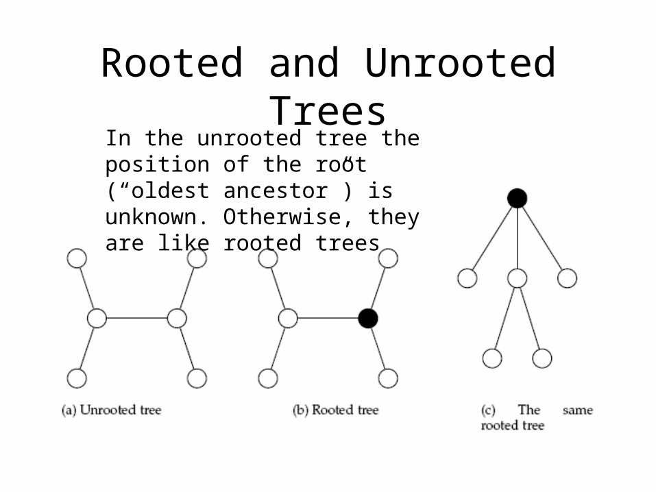
Rooted and Unrooted TreesIn the unrooted tree the position of the root (“oldest ancestor”) is unknown. Otherwise, they are like rooted trees

Distances in Trees• Edges may have weights reflecting:

– Number of mutations on evolutionary path from one species to another

– Time estimate for evolution of one species into another

• In a tree T, we often compute

dij(T) - the length of a path between leaves i and j • This may be based on direct comparison of

sequence between i and j

Distance in Trees: an Example

d1,4 = 12 + 13 + 14 + 17 + 13 = 69

i

j

Fitting Distance Matrix

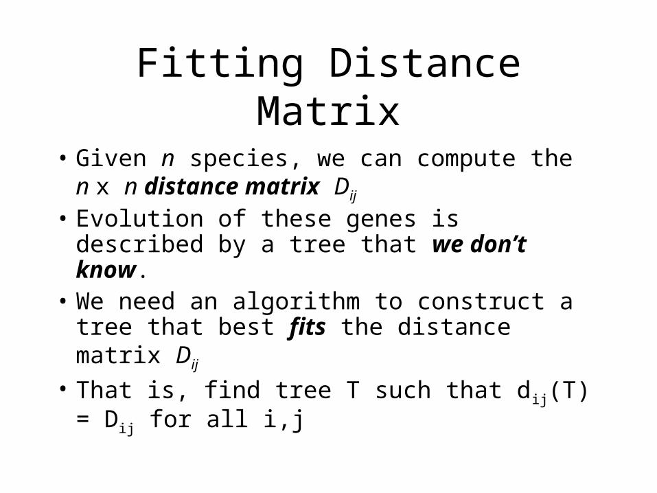
• Given n species, we can compute the n x n distance matrix Dij

• Evolution of these genes is described by a tree that we don’t know.

• We need an algorithm to construct a tree that best fits the distance matrix Dij

• That is, find tree T such that dij(T) = Dij for all i,j

Reconstructing a 3 Leaved Tree

• Tree reconstruction for any 3x3 matrix is straightforward

• We have 3 leaves i, j, k and a center vertex c

Observe:

dic + djc = Dij

dic + dkc = Dik

djc + dkc = Djk

Reconstructing a 3 Leaved Tree (cont’d)

dic + djc = Dij

dic + dkc = Dik

2dic + djc + dkc = Dij + Dik

2dic + Djk = Dij + Dik

dic = (Dij + Dik – Djk)/2Similarly,

djc = (Dij + Djk – Dik)/2dkc = (Dki + Dkj – Dij)/2

Trees with > 3 Leaves

• Any tree with n leaves has 2n-3 edges

• This means fitting a given tree to a distance matrix D requires solving a system of “n choose 2” equations with 2n-3 variables

• This is not always possible to solve for n > 3

Additive Distance Matrices

Matrix D is ADDITIVE if there exists a tree T with dij(T) = Dij

NON-ADDITIVE otherwise

Distance Based Phylogeny Problem

• Goal: Reconstruct an evolutionary tree from a distance matrix

• Input: n x n distance matrix Dij

• Output: weighted tree T with n leaves fitting D

• If D is additive, this problem has a solution and there is a simple algorithm to solve it

Solution 1

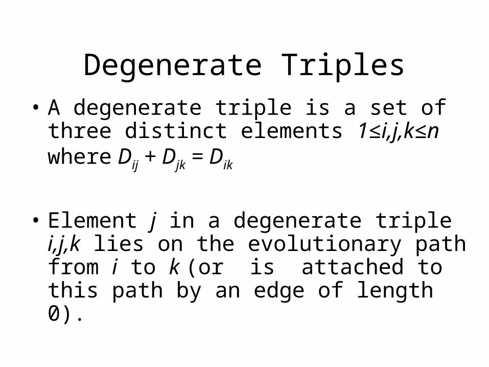
Degenerate Triples• A degenerate triple is a set of three distinct

elements 1≤i,j,k≤n where Dij + Djk = Dik

• Element j in a degenerate triple i,j,k lies on the evolutionary path from i to k (or is attached to this path by an edge of length 0).

Looking for Degenerate Triples

• If distance matrix D has a degenerate triple i,j,k then j can be “removed” from D thus reducing the size of the problem.

• If distance matrix D does not have a degenerate triple i,j,k, one can “create” a degenerate triple in D by shortening all hanging edges (edge leading to a leaf) in the tree.

Shortening Hanging Edges to Produce Degenerate Triples

• Shorten all “hanging” edges (edges that connect leaves) until a degenerate triple is found

Finding Degenerate Triples

• If there is no degenerate triple, all hanging edges are reduced by the same amount δ, so that all pair-wise distances in the matrix are reduced by 2δ.

• Eventually this process collapses one of the leaves (when δ = length of shortest hanging edge), forming a degenerate triple i,j,k and reducing the size of the distance matrix D.

• The attachment point for j can be recovered in the reverse transformations by saving Dij for each collapsed leaf.

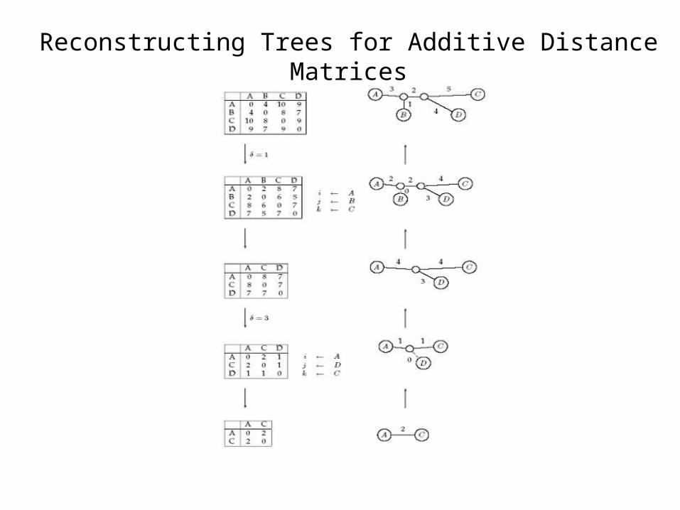
Reconstructing Trees for Additive Distance Matrices

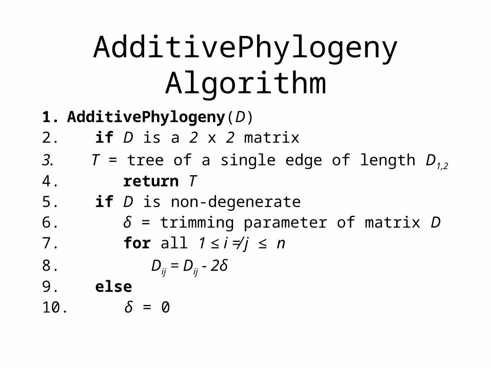
AdditivePhylogeny Algorithm

1. AdditivePhylogeny(D)2. if D is a 2 x 2 matrix3. T = tree of a single edge of length D1,2

4. return T5. if D is non-degenerate6. δ = trimming parameter of matrix D7. for all 1 ≤ i ≠ j ≤ n8. Dij = Dij - 2δ9. else10. δ = 0

AdditivePhylogeny (cont’d)

11. Find a triple i, j, k in D such that Dij + Djk = Dik

12. x = Dij

13. Remove jth row and jth column from D14. T = AdditivePhylogeny(D)15. Add a new vertex v to T at distance x from i to k16. Add j back to T by creating an edge (v,j) of length

017. for every leaf l in T18. if distance from l to v in the tree ≠ Dl,j

19. output “matrix is not additive”20. return21. Extend all “hanging” edges by length δ22. return T

AdditivePhylogeny (Cont’d)

• This algorithm checks if the matrix D is additive, and if so, returns the tree T.

• How to compute the trimming parameter δ ?

• Inefficient way to check additivity

• More efficient way comes from “Four point condition”

The Four Point Condition

• A more efficient additivity check is the “four-point condition”

• Let 1 ≤ i,j,k,l ≤ n be four distinct leaves in a tree

The Four Point Condition (cont’d)

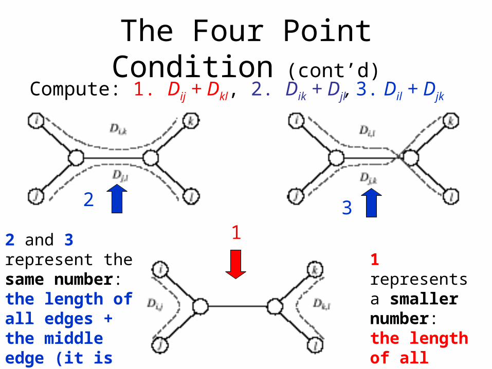
Compute: 1. Dij + Dkl, 2. Dik + Djl, 3. Dil + Djk

1

2 3

2 and 3 represent the same number: the length of all edges + the middle edge (it is counted twice)

1 represents a smaller number: the length of all edges – the middle edge

The Four Point Condition: Theorem

• The four point condition for the quartet i,j,k,l is satisfied if two of these sums are the same, with the third sum smaller than these first two

• Theorem : An n x n matrix D is additive if and only if the four point condition holds for every quartet 1 ≤ i,j,k,l ≤ n

Solution 2

UPGMA: Unweighted Pair Group Method with Arithmetic Mean

• UPGMA is a clustering algorithm that:

– computes the distance between clusters using average pairwise distance

– assigns a height to every vertex in the tree

UPGMA’s Weakness

• The algorithm produces an ultrametric tree : the distance from the root to any leaf is the same

• UPGMA assumes a constant molecular clock: all species represented by the leaves in the tree are assumed to accumulate mutations (and thus evolve) at the same rate. This is a major pitfall of UPGMA.

UPGMA’s Weakness: Example

2

3

41

1 4 32

Correct treeUPGMA

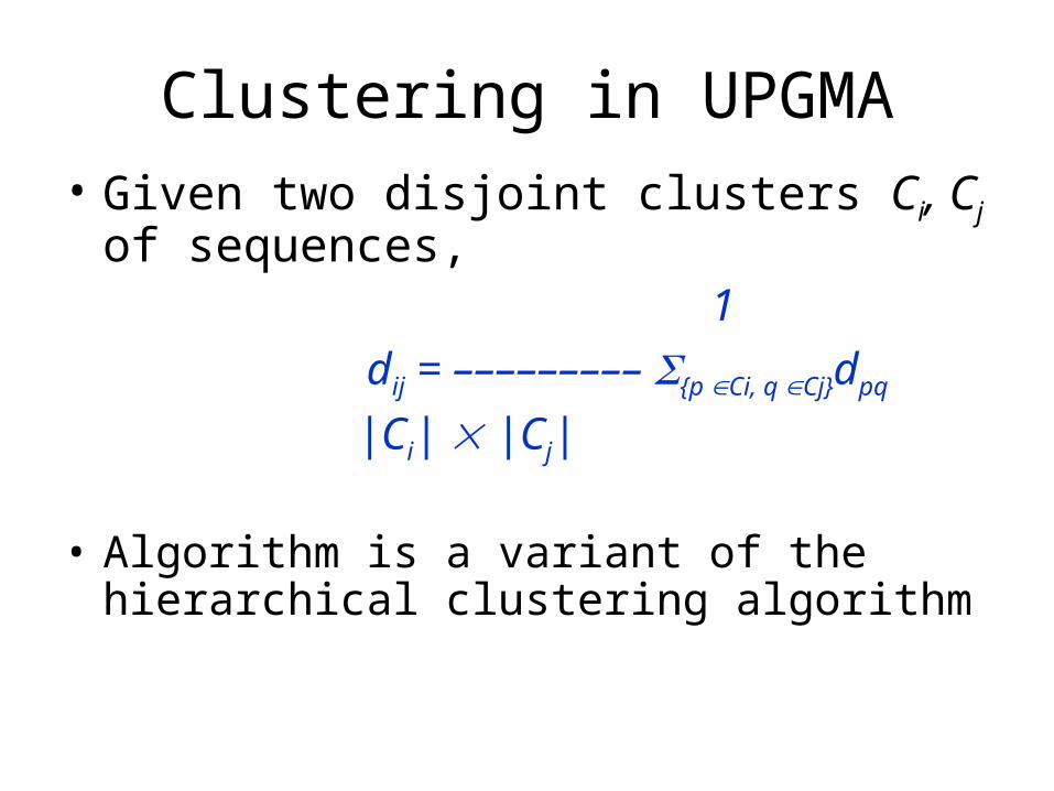
Clustering in UPGMA• Given two disjoint clusters Ci, Cj of

sequences, 1

dij = ––––––––– {p Ci, q Cj}dpq

|Ci| |Cj|

• Algorithm is a variant of the hierarchical clustering algorithm

UPGMA Algorithm

Initialization:

Assign each xi to its own cluster Ci

Define one leaf per sequence, each at height 0Iteration:

Find two clusters Ci and Cj such that dij is min

Let Ck = Ci Cj

Add a vertex connecting Ci, Cj and place it at height dij /2

Length of edge (Ci,Ck) = h(Ck) - h(Ci)

Length of edge (Cj,Ck) = h(Ck) - h(Cj)

Delete clusters Ci and Cj

Termination:When a single cluster remains

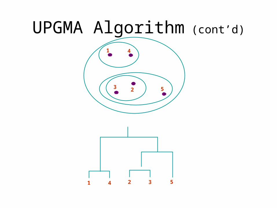
UPGMA Algorithm (cont’d)

1 4

3 2 5

1 4 2 3 5

Solution 3

Using Neighboring Leaves to Construct the Tree

• Find neighboring leaves i and j with parent k• Remove the rows and columns of i and j• Add a new row and column corresponding to k, where

the distance from k to any other leaf m can be computed as:

Dkm = (Dim + Djm – Dij)/2

Compress i and j into k, iterate algorithm for rest of tree

Finding Neighboring Leaves• To find neighboring leaves we simply select a pair of closest leaves.

• WRONG !

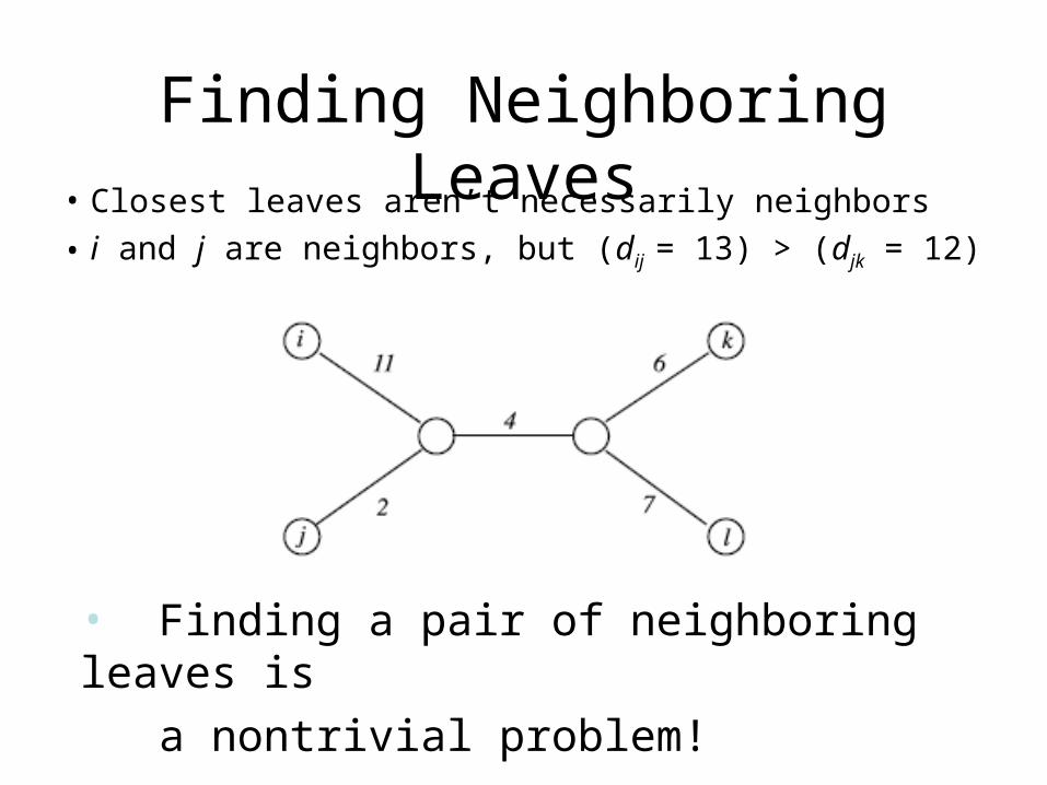
Finding Neighboring Leaves• Closest leaves aren’t necessarily neighbors

• i and j are neighbors, but (dij = 13) > (djk = 12)

• Finding a pair of neighboring leaves is

a nontrivial problem!

Neighbor Joining Algorithm

• In 1987 Naruya Saitou and Masatoshi Nei developed a neighbor joining algorithm for phylogenetic tree reconstruction

• Finds a pair of leaves that are close to each other but far from other leaves: implicitly finds a pair of neighboring leaves

• Similar to UPGMA, merges clusters iteratively• Finds two clusters that are closest to each other and

farthest from the other clusters• Advantages: works well for additive and other non-

additive matrices, it does not have the flawed molecular clock assumption

Solution 4

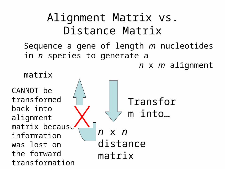
Alignment Matrix vs. Distance Matrix

Sequence a gene of length m nucleotides in n species to generate a               n x m alignment matrix

n x n distance matrix

CANNOT be transformed back into alignment matrix because information was lost on the forward transformation

Transform into…

Character-Based Tree Reconstruction

• Better technique:– Character-based reconstruction algorithms

use the n x m alignment matrix

(n = # species, m = #characters)

directly instead of using distance matrix. – GOAL: determine what character strings at

internal nodes would best explain the character strings for the n observed species

Character-Based Tree Reconstruction (cont’d)

• Characters may be nucleotides, where A, G, C, T are states of this character. Other characters may be the # of eyes or legs or the shape of a beak or a fin.

• By setting the length of an edge in the tree to the Hamming distance, we may define the parsimony score of the tree as the sum of the lengths (weights) of the edges

Parsimony Approach to Evolutionary Tree Reconstruction

• Applies Occam’s razor principle to identify the simplest explanation for the data

• Assumes observed character differences resulted from the fewest possible mutations

• Seeks the tree that yields lowest possible parsimony score - sum of cost of all mutations found in the tree

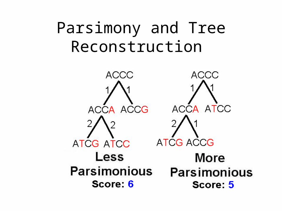
Parsimony and Tree Reconstruction

Small Parsimony Problem

• Input: Tree T with each leaf labeled by an m-character string.

• Output: Labeling of internal vertices of the tree T minimizing the parsimony score.

• We can assume that every leaf is labeled by a single character, because the characters in the string are independent.

Weighted Small Parsimony Problem

• A more general version of Small Parsimony Problem

• Input includes a k * k scoring matrix describing the cost of transformation of each of k states into another one

• For Small Parsimony problem, the scoring matrix is based on Hamming distance

dH(v, w) = 0 if v=w

dH(v, w) = 1 otherwise

Scoring Matrices

A T G C

A 0 1 1 1

T 1 0 1 1

G 1 1 0 1

C 1 1 1 0

A T G C

A 0 3 4 9

T 3 0 2 4

G 4 2 0 4

C 9 4 4 0

Small Parsimony Problem Weighted Parsimony Problem

Weighted Small Parsimony Problem: Formulation

• Input: Tree T with each leaf labeled by elements of a k-letter alphabet and a k x k scoring matrix (ij)

• Output: Labeling of internal vertices of the tree T minimizing the weighted parsimony score

Sankoff’s Algorithm

• Check children’s every vertex and determine the minimum between them

• An example

Sankoff Algorithm: Dynamic Programming

• Calculate and keep track of a score for every possible label at each vertex– st(v) = minimum parsimony score of the

subtree rooted at vertex v if v has character t

• The score at each vertex is based on scores of its children:

– st(parent) = mini {si( left child ) + i, t} +

minj {sj( right child ) + j, t}

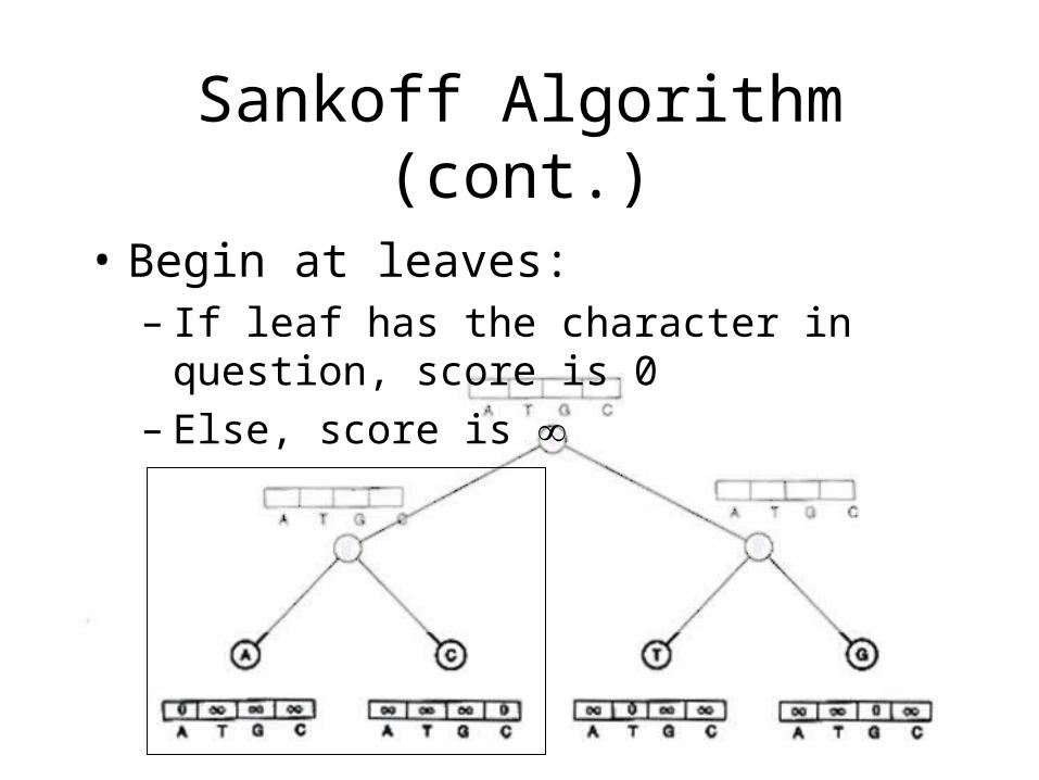
Sankoff Algorithm (cont.)

• Begin at leaves:– If leaf has the character in question, score

is 0– Else, score is

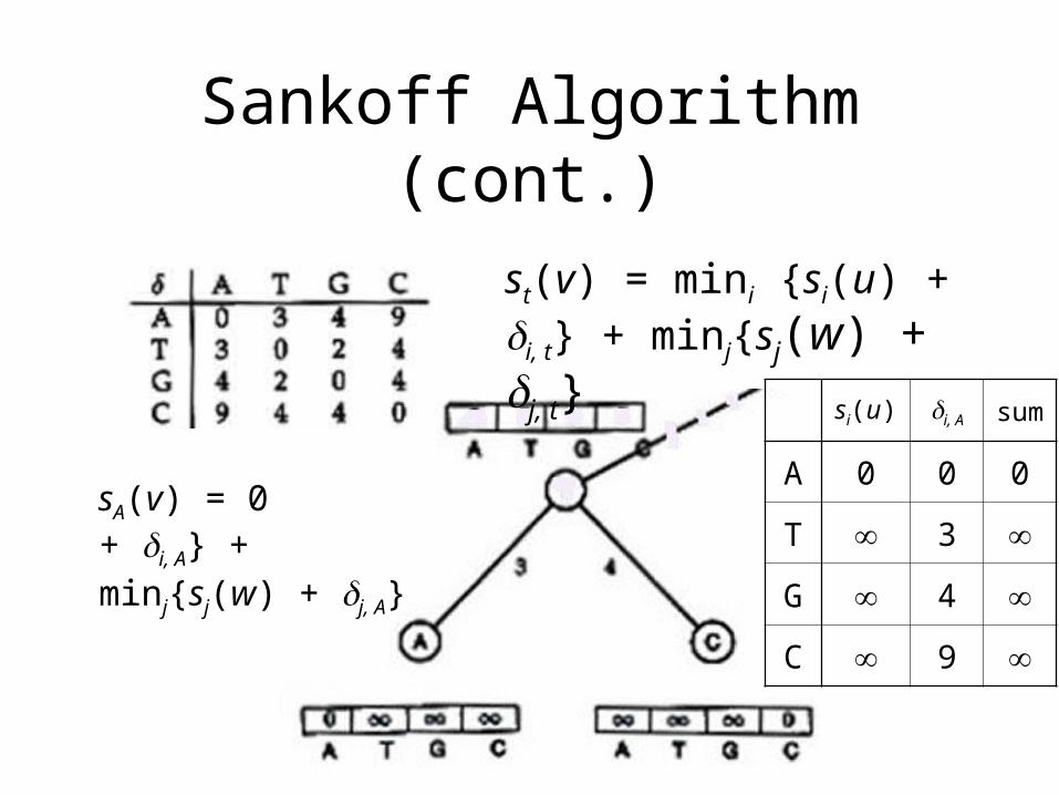
Sankoff Algorithm (cont.)

st(v) = mini {si(u) + i, t} + minj{sj(w) + j, t}

sA(v) = mini{si(u) + i, A} + minj{sj(w) + j, A}

si(u) i, A sum

A 0 0 0

T 3

G 4

C 9

sA(v) = 0

Sankoff Algorithm (cont.)

st(v) = mini {si(u) + i, t} + minj{sj(w) + j, t}

sA(v) = mini{si(u) + i, A} + minj{sj(w) + j, A}

sj(u) j, A sum

A 0

T 3

G 4

C 0 9 9

+ 9 = 9sA(v) = 0

Sankoff Algorithm (cont.)

st(v) = mini {si(u) + i, t} + minj{sj(w) + j, t}

Repeat for T, G, and C

Sankoff Algorithm (cont.)

Repeat for right subtree

Sankoff Algorithm (cont.)

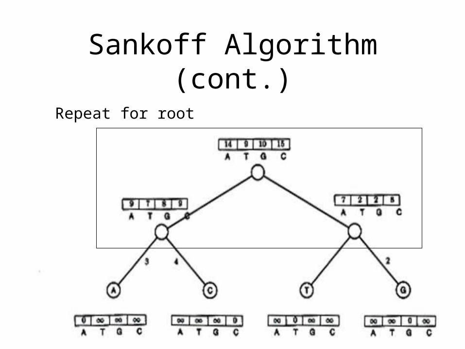
Repeat for root

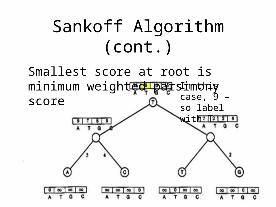
Sankoff Algorithm (cont.)

Smallest score at root is minimum weighted parsimony score In this case, 9 –

so label with T

Sankoff Algorithm: Traveling down the Tree

• The scores at the root vertex have been computed by going up the tree

• After the scores at root vertex are computed the Sankoff algorithm moves down the tree and assign each vertex with optimal character.

Sankoff Algorithm (cont.)

9 is derived from 7 + 2

So left child is T,

And right child is T

Sankoff Algorithm (cont.)

And the tree is thus labeled…

Large Parsimony Problem

• Input: An n x m matrix M describing n species, each represented by an m-character string

• Output: A tree T with n leaves labeled by the n rows of matrix M, and a labeling of the internal vertices such that the parsimony score is minimized over all possible trees and all possible labelings of internal vertices

Large Parsimony Problem (cont.)

• Possible search space is huge, especially as n increases– (2n – 3)!! possible rooted trees– (2n – 5)!! possible unrooted trees

• Problem is NP-complete– Exhaustive search only possible w/ small n(< 10)

• Hence, branch and bound or heuristics used

Nearest Neighbor InterchangeA Greedy Algorithm

• A Branch Swapping algorithm• Only evaluates a subset of all possible trees• Defines a neighbor of a tree as one reachable

by a nearest neighbor interchange– A rearrangement of the four subtrees defined by

one internal edge– Only three different arrangements per edge