EVOLUTIONARY STRUCTURAL OPTIMIZATION WITH MULTIPLE PERFORMANCE CONSTRAINTS BY LARGE ADMISSIBLE PERTURBATIONS by Taemin Earmme A dissertation submitted in partial fulfillment of the requirements for the degree of Doctor of Philosophy (Mechanical Engineering and Naval Architecture and Marine Engineering) in The University of Michigan 2009 Doctoral Committee: Professor Michael M. Bernitsas, Co-Chair Professor Panos Y. Papalambros, Co-Chair Professor Armin W. Troesch Associate Professor Dale G. Karr

Welcome message from author
This document is posted to help you gain knowledge. Please leave a comment to let me know what you think about it! Share it to your friends and learn new things together.
Transcript
EVOLUTIONARY STRUCTURAL OPTIMIZATION WITH MULTIPLE PERFORMANCE CONSTRAINTS BY LARGE ADMISSIBLE
PERTURBATIONS
by
Taemin Earmme
A dissertation submitted in partial fulfillment of the requirements for the degree of
Doctor of Philosophy (Mechanical Engineering and Naval Architecture and Marine Engineering)
in The University of Michigan 2009
Doctoral Committee: Professor Michael M. Bernitsas, Co-Chair Professor Panos Y. Papalambros, Co-Chair Professor Armin W. Troesch Associate Professor Dale G. Karr

© Taemin Earmme
2009

ii
To My Parents

iii
ACKNOWLEDGEMENTS
I would like to thank my advisor, Professor Michael Bernitsas for his valuable
advice and guidance throughout my graduate work. I also like to express sincere
appreciation to the members of my dissertation committee, Professor Papalambros,
Professor Troesch and Professor Karr, especially thankful to Professor Papalambros who
accepted a position as co-chair of my combined Ph.D.
Thanks to all of my friends in Mechanical Engineering who started this long
journey together. I will never forget the days spent with everyone. I really appreciate
seniors and friends in Naval Architecture and Marine Engineering who welcomed me
with warm hearts and support when I joined the NAME department. Also, thanks to my
good old friends in GLC (Gainax Lover's Club) for their support of all the stress relieving
things.
I have been fortunate to have officemates, Jonghun and Ayoung sitting side by
side – helping each other, talking or sometimes sharing the virtue of procrastination.
Thanks.
Finally, I would like to thank my parents and twin brother for all of the love and
support they have given me through my graduate years. Without their encouragement and
belief in me, I could not have made this far. Thank you so much.
This research was funded by NDSEG (National Defense Science and Engineering
Graduate) fellowship awarded through Department of Defense.

iv
TABLE OF CONTENTS
DEDICATION ............................................................................................. ii
ACKNOWLEDGEMENTS ....................................................................... iii
LIST OF TABLES ..................................................................................... vii
LIST OF FIGURES .................................................................................. viii
LIST OF APPENDICES ............................................................................. xi
NOMENCLATURE ................................................................................... xii
ABSTRACT ................................................................................................ xiv
CHAPTER
I. INTRODUCTION ............................................................................ 1
1.1. Literature Review ......................................................................................2
1.1.1. Topology Optimization .................................................................2
1.1.2. Evolutionary Structural Optimization ...........................................3
1.1.3. LargE Admissible Perturbation (LEAP) Methodology ................3
1.2. Dissertation Outline .....................................................................................4
II. PROBLEM FORMULATION ....................................................... 6
2.1. Topology Optimization Formulation .........................................................6
2.2. LargE Admissible Perturbation (LEAP) Formulation ...............................9
2.3. Evolutionary Structural Optimization (ESO) Algorithm .........................15
2.3.1. Element Elimination Criterion ....................................................15
v
2.3.2. Cumulative Energy Elimination Rate (CEER) ...........................17
2.3.3. Element Freezing Criterion .........................................................18
2.4. Optimization Process Steps .....................................................................18
III. PARAMETRIC EVOLUTION RESULTS ............................... 22
3.1. Static Displacement Problem ...................................................................25
3.1.1. Cantilever Beam ..........................................................................25
3.1.2. Bridge ..........................................................................................27
3.2. Modal Dynamic Problem .........................................................................29
3.2.1. Cantilever Beam ...........................................................................29
3.2.2. Bridge ..........................................................................................31
3.3. Simultaneous Static and Modal Dynamic Problem ..................................33
3.3.1. Cantilever Beam ...........................................................................33
3.3.2. Bridge ..........................................................................................35
3.4. Topology Evolution with Increased Resolution ......................................38
3.5. Topology Evolution with Performance Constraints Varied .....................40
3.5.1. Static Displacement Constraints .................................................40
3.5.2. Modal Dynamic Constraints .......................................................43
IV. TOPOLOGY EVOLUTION PATTERNS ................................. 46
4.1. Static Displacement Topology Evolution Patterns ...................................46
4.1.1. Cantilever Beam ..........................................................................46
4.1.2. Bridge ..........................................................................................50
4.2. Modal Dynamic Topology Evolution Patterns ........................................54
4.2.1. Cantilever Beam ..........................................................................54
4.2.2. Bridge ..........................................................................................59
4.3. Static and Modal Dynamic Topology Evolution Patterns ........................62
4.3.1. Cantilever Beam ..........................................................................62
4.3.2. Bridge ..........................................................................................68
V. CONCLUSIONS .......................................................................... 72

vi
5.1. Dissertation Contributions .......................................................................72
5.2. Concluding Remarks ................................................................................74
5.3. Suggested Future Work ...........................................................................75
APPENDICES ............................................................................................. 76
BIBLOGRAPHY ........................................................................................ 88
vii
LIST OF TABLES
Table
3.1. Structural performance specifications for cantilever beam application ...................24
3.2. Structural performance specifications for bridge application ..................................24
3.3. Number of iterations and volume reduction percentage for static cantilever beam
evolution ..................................................................................................................26
3.4. Number of iterations and volume reduction percentage for static bridge
evolution ..................................................................................................................28
3.5. Number of iterations and volume reduction percentage for modal dynamic
cantilever beam evolution ........................................................................................30
3.6. Number of iterations and volume reduction percentage for modal dynamic
bridge evolution .......................................................................................................32
3.7. Number of iterations and volume reduction percentage for static displacement
and modal dynamic of cantilever beam evolution ...................................................34
3.8. Number of iterations and volume reduction percentage for static displacement
and modal dynamic bridge evolution .......................................................................36
3.9. Number of iterations and volume reduction for the high resolution
cantilever beam evolution ........................................................................................39
3.10. Number of iterations and volume reduction for static displacement
objective of cantilever beam evolution with lower corner force .............................43
3.11. Number of iterations and volume reduction for modal dynamic
objective of cantilever beam evolution ....................................................................45

viii
LIST OF FIGURES
Figure
2.1. Schematic representation of solution process ..........................................................11
2.2. Algorithmic Representation of Incremental Method ...............................................14
2.3. Algorithmic Representation of ESO/LEAP(Evolutionary Structural
Optimization/ LargE Admissible Perturbation) methodology .................................20
3.1. Cantilever beam with one point load at the center of the free-end ..........................22
3.2. Bridge with three point loads ...................................................................................23
3.3. Evolved cantilever beam for static displacement objective and sE = 3.0 ...............26
3.4. Evolved cantilever beam for static displacement objective and sE = 3.5 ...............26
3.5. Evolved bridge for static displacement objective and sE = 3.0 ..............................28
3.6. Evolved bridge for static displacement objective and sE = 3.5 ..............................28
3.7. Evolved cantilever beam for modal dynamic objective and sE = 3.0 .....................30
3.8. Evolved cantilever beam for modal dynamic objective and sE = 3.5 .....................30
3.9. Evolved bridge for modal dynamic objective and sE = 3.0 ....................................32
3.10. Evolved bridge for modal dynamic objective and sE = 3.5 ....................................32
3.11. Evolved cantilever beam for static displacement/modal dynamic objective
and sE = 3.0 ............................................................................................................34
3.12. Evolved cantilever beam for static displacement/modal dynamic objective
and sE = 3.5 ............................................................................................................34
3.13. Evolved bridge for static displacement/modal dynamic objective
and sE = 2.0 ............................................................................................................36
3.14. Evolved bridge for static displacement/modal dynamic objective
and sE = 2.5 ............................................................................................................36

ix
3.15. Evolved cantilever beam for static displacement objective with high resolution ....39
3.16. Evolved cantilever beam for modal dynamic objective with high resolution .........39
3.17. Cantilever beam with one point load at the lower corner of the free-end ................40
3.18. Evolved cantilever beam with lower corner force for static displacement
objective / 0.5u u′ = .................................................................................................42
3.19. Evolved cantilever beam with lower corner force for static displacement
objective / 0.65u u′ = ...............................................................................................42
3.20. Evolved cantilever beam with lower corner force for static displacement
objective / 0.8u u′ = .................................................................................................42
3.21. Evolved cantilever beam for modal dynamic objective 2 2/ 1.44ω ω′ = ...................44
3.22. Evolved cantilever beam for modal dynamic objective 2 2/ 1.6ω ω′ = .....................44
3.23. Evolved cantilever beam for modal dynamic objective 2 2/ 1.8ω ω′ = .....................44
4.1. Topology evolution pattern for cantilever beam - static displacement objective
and sE =3.0 ..............................................................................................................48
4.2. Topology evolution pattern for cantilever beam - static displacement objective
and sE =3.5 ..............................................................................................................49
4.3. Topology evolution pattern for bridge - static displacement objective
and sE =3.0 ..............................................................................................................51
4.4. Topology evolution pattern for bridge - static displacement objective
and sE =3.5 ..............................................................................................................53
4.5. Topology evolution pattern for cantilever beam – modal dynamic objective
and sE =3.0 ..............................................................................................................56
4.6. Topology evolution pattern for cantilever beam – modal dynamic objective
and sE =3.5 ..............................................................................................................58
4.7. Topology evolution pattern for bridge – modal dynamic objective
and sE =3.0 ..............................................................................................................60
4.8. Topology evolution pattern for bridge – modal dynamic objective
and sE =3.5 ..............................................................................................................61
x
4.9. Topology evolution pattern for cantilever beam – static displacement/modal
dynamic objectives and sE =3.0 ..............................................................................64
4.10. Topology evolution pattern for cantilever beam – static displacement/modal
dynamic objectives and sE =3.5 ..............................................................................67
4.11. Topology evolution pattern for bridge – static displacement/modal
dynamic objectives and sE =2.0 ..............................................................................69
4.12. Topology evolution pattern for bridge – static displacement/modal
dynamic objectives and sE =2.5 ..............................................................................71

xi
LIST OF APPENDICES
APPENDIX
A. General Perturbation Equation for Static Deflection with
Static Mode Compensation ......................................................................................... 76
(a) Static Mode Compensation .....................................................................................76
(b) General Perturbation Equation for Static Deflection Redesign .............................78
B. General Perturbation Equation for Modal Dynamics ...................................................80
C. Linear Prediction for Eigenvectors ..............................................................................82
D. Feasible Sequential Quadratic Programming (FSQP) .................................................85

xii
NOMENCLATURE
Symbol Description [ ]eB element strain-nodal displacement matrix
CEER Cumulative Energy Elimination Rate
[ ]eD element constitutive law matrix
DSE Dynamic Strain Energy
e e -th redesign variable ( 1, ,e p= … )
E Young’s modulus
0E initial Young’s modulus
eE element Young’s modulus
sE designer specified (target) Young’s modulus
{ }f force vector
[ ]k global stiffness matrix
[ ]ek element stiffness matrix
[ ]K generalized stiffness matrix
KE Kinetic Energy
l increment number
LEAP LargE Admissible Perturbations
[ ]m global mass matrix
[ ]em element mass matrix
[ ]M generalized mass matrix
n number of degrees of freedom of structural model
an number of admissibility constraints
xiii
[ ]eN interpolation function matrix for element
rn number of the extracted modal dynamic modes
un number of displacement constraints
nω number of natural frequency constraints
dn number of forced response amplitude constraints
nσ number of static stress constraints
p number of redesign variables
RESTRUCT REdesign of STRUCTures program
s calculated performance value
s′ performance objective value
S1 baseline (initial) structure
S2 unknown (objective) structure
SSE Static Strain Energy
{ }u nodal displacement vector
eU equivalent energy level for element
Greek Symbols eα fractional change of redesign variable
∆ change between state S1 and state S2
[ ]Φ dynamic mode shape matrix
{ }iφ i -th dynamic mode shape vector
2iω i -th modal dynamic eigenvalue
Special Symbols
( )′ refers to desired structure
[ ] { },T T transposed matrix and vector, respectively
( )l refers to l -th increment in the incremental scheme

xiv
ABSTRACT
EVOLUTIONARY STRUCTURAL OPTIMIZATION WITH MULTIPLE PERFORMANCE CONSTRAINTS BY LARGE ADMISSIBLE
PERTURBATIONS
by
Taemin Earmme Co-Chairs: Michael M. Bernitsas and Panos Y. Papalambros
A LargE Admissible Perturbation (LEAP) with Evolutionary Structural
Optimization methodology is developed. The LEAP methodology uses an incremental
predictor-corrector scheme, which makes it possible to solve the redesign problem using
data only from the finite element analysis of the baseline structure for changes on the
order of 100% in performance and redesign variables without trial and error or repetitive
finite element analyses. A structural topology evolution algorithm is introduced using a
Cumulative Energy Elimination Rate (CEER) scheme by removing low energy elements
at each iteration, while using the elastic modulus in each element as redesign variable in
the LEAP methodology. Benchmark examples are used to demonstrate that static
displacement, modal dynamic constraints, and simultaneous static and dynamic
constraints can be achieved. Convergence is achieved in 3 to 7 iterations with two FEA’s
per iteration inside the ESO/LEAP algorithm. Results of numerical applications satisfy
engineering intuition and show the effect of multiple objectives on topology evolution.

1
CHAPTER I
INTRODUCTION
A designer knows he has achieved perfection not when there is nothing left to add,
but when there is nothing left to take away. (Antoine de Saint-Exupéry)
For decades, the development of Finite Element Analysis (FEA) has played an
important role design various and complex structures along with the achievement of
computational efficiency. The area of structural optimization has expanded with the
advancement of Finite Element Analysis (FEA) in various industry fields from
automotive to electronics, mostly designing the mechanical elements and devices. The
structural optimization techniques played a major role to obtain a best solution satisfying
any engineering specification required by a designer.
Structural optimization can be largely classified into three main areas: size
optimization, shape optimization and topology optimization. In size optimization, the
goal is to find the optimal thickness distribution of a linearly elastic plate or the optimal
member areas in a truss structure. The design domain and the topology of the structure
are fixed while changing the size to achieve the design objective. In shape optimization,
the boundary of a given topology varies to obtain optimal shape. In a typical case of
shape optimization such as the boundary variation method, the objective is to refine the
initial shape to an optimized shape, which achieves minimal von Mises equivalent stress
in the body.
Topology optimization concentrates on the distribution of material and structural
connectivity in the design domain. It aims finding an optimal lay-out of the structure,
2
which maximizes (or minimizes) an efficiency measure subjected to specific constraints.
The importance of topology optimization is growing to a greater extent recently,
since it can provide intuitive concepts to a designer at the early stage of the designing
process.
1.1. Literature Review
In Section 1.1.1, the development of general Topology Optimization is reviewed
with two major approaches: Homogenization method and Solid Isotropic Material
Penalization. Evolutionary Structural Optimization (ESO) related papers are presented in
Section 1.1.2 and a development history of LargE Admissible Perturbations (LEAP)
methodology is reviewed in Section 1.1.3.
1.1.1. Topology Optimization
Topology optimization is first developed from distributed parameter approaches
to shape optimization. Cheng and Olhoff [1] identified that the zero thickness of a plate
implies void material in the structure. Their work led to Bendsøe and Kikuchi [2] who
first introduced the material distribution for topology design as a computational tool.
Most of topology structural optimization problem frequently studied is the
compliance minimization (stiffness maximization) subject to volume constraints. There
are two approaches to this problem: the one is the homogenization method and the other
is SIMP (Solid Isotropic with Material Penalization) method.
Homogenization Method
In the homogenization method, a homogenized elasticity tensor is formulated to
model a unit cell with a rectangular void. (Bendsøe & Kikuchi [2], Bendsøe [3]) The
dimensions and orientation angles of the voids are used as the design variables. The
initial design domain is homogeneous at the macroscopic scale and the size and
orientation of internal rectangular holes are varied to find optimal porosity of the
3
structure. The method has been successfully applied to solve many types of topology
optimization problems (Suzuki [4], Ma & Kikuchi [5], Pederson [6]).
SIMP(Solid Isotropic with Material Penalization) Method
The SIMP (Solid Isotropic with Material Penalization) method is the most widely
used minimum compliance formulation. It implements the idea of a penalizing density
variable to converge to zero or one, i.e., void or solid (Yang & Chuang [7]). One of the
advantages of the SIMP formulation is that it is easy to implement in a Finite Element
Analysis framework.
1.1.2. Evolutionary Structural Optimization
Evolutionary Structural Optimization (ESO) was first introduced by Xie and
Steven [8] by gradually removing the low stress elements to obtain the objective structure.
It has been applied to many individual optimization criteria such as stress, strain, stiffness,
natural frequency, buckling, stress minimization, and heat transfer (Chu et al.[9], Zhao,
Steven & Xie [10], Manickarajah, Xie & Steven [11], Li et al.[12]) .
The ESO methodology is expanded to Bi-directional Evolutionary Structural
Optimization (BESO) (Querin et al.[13], Proos et al.[14], Huang & Xie [15]). The BESO
approach allows both removing and adding elements which leads to the optimum more
efficiently. BESO methodology was used to design continuum structures with one or
multiple materials, or periodic structures utilizing the material interpolation scheme
(Huang & Xie [16],[17]).
1.1.3. LargE Admissible Perturbation (LEAP) Methodology
Perturbation based redesign methods have been introduced by Stetson and Palma
[18]. They used linear perturbation method to calculate small structural changes
necessary which affect the given change in vibration modes. Sandström and Anderson
4
[19] and Stetson and Harrison [20] developed equations that relate the unknown
eigenvectors of the desired structure to the known eigenvectors of the initial structure.
The LargE Admissible Perturbation (LEAP) methodology was first developed to
formulate and solve the structural redesign problem. It can solve large scale redesign
problems subject to static displacement, natural frequency, forced dynamics amplitude,
and static stress constraints. LEAP can achieve changes on the order of 100%-300%
without trial and error or repeated finite element analyses. Hoff and Bernitsas [21]
introduced static and modal dynamic redesign. The two constraints were integrated in the
redesign process by Kim and Bernitsas [22]. Bernitsas and Tawekal [23] solved the
model calibration problem by LEAP in a cognate space. Plate and shell elements were
added by Bernitsas and Rim [24]. Bernitsas and Suryatama [25] improved the static
deflection redesign algorithm by introducing static mode compensation. Bernitsas and
Blouin [26] developed a LEAP algorithm to solve the problem of forced response
amplitude. The static stress redesign problem was solved by Bernitsas and by Kristanto
[27]. Blouin and Bernitsas [28] developed and compared incremental and direct methods
for the LEAP algorithm.
The LEAP methodology was first implemented in topology optimization by
Suryatama and Bernitsas [29] optimizing a structure which satisfied several performance
constraints simultaneously. This was further developed and studied by Miao and
Bernitsas [30] and Earmme and Bernitsas [31] using the Evolutionary Structural
Optimization method.
1.2. Dissertation Outline
In this dissertation, a structural topology evolution algorithm is developed using
LargE Admissible Perturbations (LEAP). The problem formulation for general topology
optimization and LargE Admissible Perturbations methodology is described in Chapter II.
The general topology optimization is formulated in Section 2.1 and LEAP methodology
is presented in Section 2.2.
In Section 2.3, an Evolutionary Structural Optimization scheme is described. The
ESO/LEAP algorithm consists of two nested loops. The outer loop is the process of

5
removal of inefficient elements while the inner loop uses LEAP to find the optimal
design which satisfies the performance objectives. The elastic modulus in each element is
used as redesign variable in the LEAP methodology. A Cumulative Energy Elimination
Rate (CEER) scheme is introduced by removing low energy elements, which do not
contribute to total performance of the structure, at each iteration.
In Chapter III, the developed methodology is tested by two benchmark examples:
cantilever beam and bridge. The numerical results for static displacement, modal
dynamic, and simultaneous static displacement and modal dynamic performance
constraints are presented from Section 3.1 through Section 3.3. The results for cantilever
beam example with increased finite element mesh is exhibited in Section 3.4 and the
converged results for varying the value of performance constraints are shown in Section
3.5.
The detailed evolution pattern is further studied in Chapter IV. The evolving
topology progress of benchmark example is shown to verify the effectiveness of present
methodology. The dissertation contributions/conclusions and suggested future work are
summarized in Chapter V.
6
CHAPTER II
PROBLEM FORMULATION
This Chapter consists of two parts, the first one is the general topology
optimization formulation and the second recasts that formulation into a Large Admissible
Perturbation form. Those are presented in Sections 2.1 and 2.2, respectively.
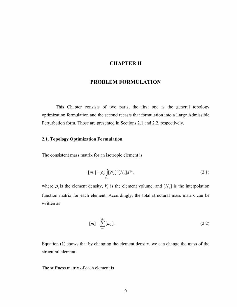
2.1. Topology Optimization Formulation
The consistent mass matrix for an isotropic element is
[ ] [ ] [ ]e
Te e e e
V
m N N dVρ= ∫ , (2.1)
where eρ is the element density, eV is the element volume, and [ ]eN is the interpolation
function matrix for each element. Accordingly, the total structural mass matrix can be
written as
1[ ] [ ]
en
ee
m m=
=∑ . (2.2)
Equation (1) shows that by changing the element density, we can change the mass of the
structural element.
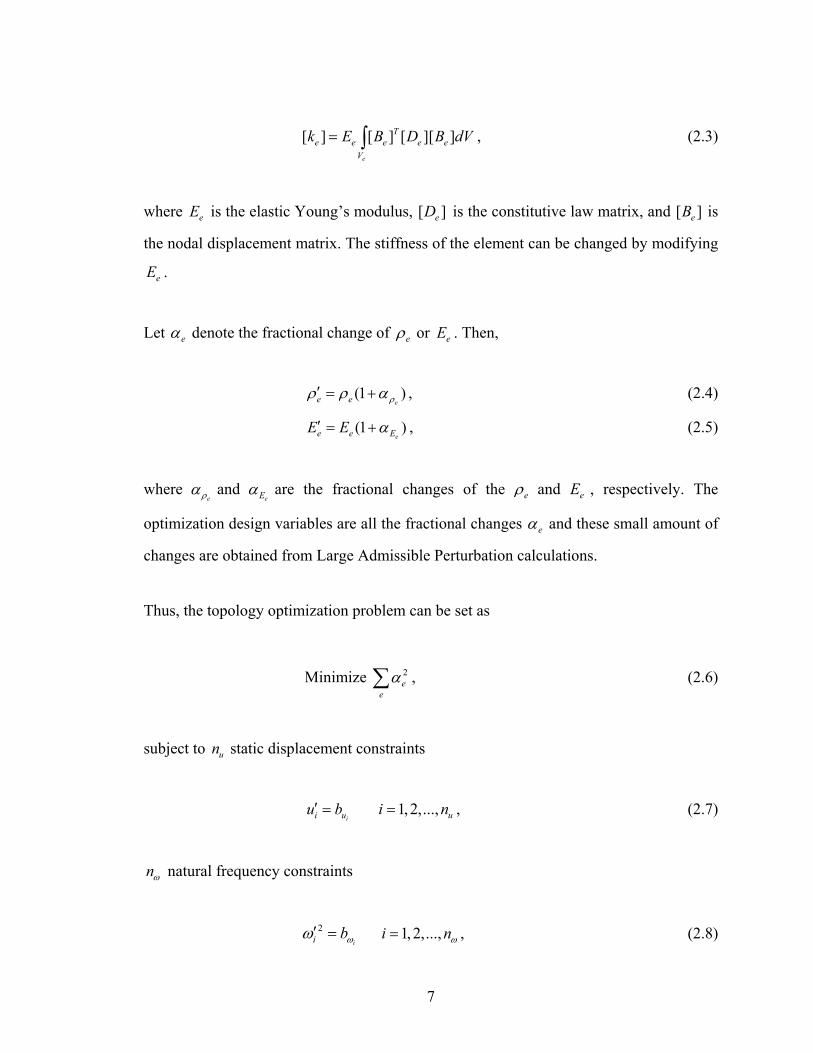
The stiffness matrix of each element is
7
[ ] [ ] [ ][ ]e
Te e e e e
V
k E B D B dV= ∫ , (2.3)
where eE is the elastic Young’s modulus, [ ]eD is the constitutive law matrix, and [ ]eB is
the nodal displacement matrix. The stiffness of the element can be changed by modifying
eE .
Let eα denote the fractional change of eρ or eE . Then,
(1 )ee e ρρ ρ α′ = + , (2.4)
(1 )ee e EE E α′ = + , (2.5)
where eρ
α and eEα are the fractional changes of the eρ and eE , respectively. The
optimization design variables are all the fractional changes eα and these small amount of
changes are obtained from Large Admissible Perturbation calculations.
Thus, the topology optimization problem can be set as
Minimize 2e
eα∑ , (2.6)
subject to un static displacement constraints
ii uu b′ = 1, 2,..., ui n= , (2.7)
nω natural frequency constraints
2
ii bωω′ = 1, 2,...,i nω= , (2.8)

8
dn forced-response amplitude constraints
ii dd b′ = 1, 2,..., di n= , (2.9)
nσ static stress constraints
ii bσσ ′ = 1, 2,...,i nσ= , (2.10)
where , ,u db b bω , and bσ are the designer performance specifications. Primed quantities
refer to the objective structure while unprimed quantities refer to the initial baseline
structure. Further, an admissibility constraints are imposed from among the complete set
{ } [ ]{ } 0Tj ikφ φ′ ′ ′ = , (2.11)
{ } [ ]{ } 0Tj imφ φ′ ′ ′ = , 1, 2,...,i nω= , 1,..., rj i n= + , (2.12)
and 2p lower and upper bounds on the redesign variables are imposed
1 ,e e eα α α− +− < ≤ ≤ 1, 2,...,e p= , (2.13)
where eα is element redesign variable, p is the number of redesign variables, eα− , eα
+ are
lower and upper bound, respectively. Material specifications on the redesign variables are
0eE = or sE . (2.14)
The optimization criterion here is the norm of the difference between initial
structure and objective structure instead of minimization of compliance which is usually
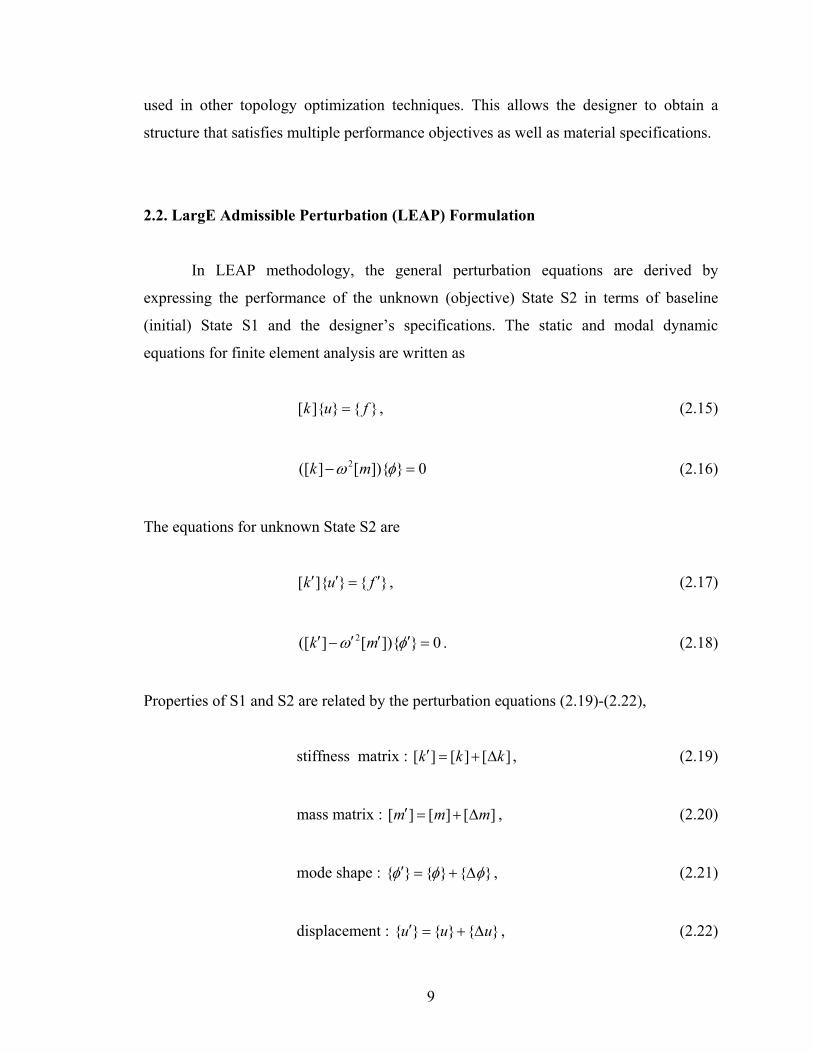
9
used in other topology optimization techniques. This allows the designer to obtain a
structure that satisfies multiple performance objectives as well as material specifications.
2.2. LargE Admissible Perturbation (LEAP) Formulation
In LEAP methodology, the general perturbation equations are derived by
expressing the performance of the unknown (objective) State S2 in terms of baseline
(initial) State S1 and the designer’s specifications. The static and modal dynamic
equations for finite element analysis are written as
[ ]{ } { }k u f= , (2.15)
2([ ] [ ]){ } 0k mω φ− = (2.16)
The equations for unknown State S2 are
[ ]{ } { }k u f′ ′ ′= , (2.17)
2([ ] [ ]){ } 0k mω φ′ ′ ′ ′− = . (2.18)
Properties of S1 and S2 are related by the perturbation equations (2.19)-(2.22),
stiffness matrix : [ ] [ ] [ ]k k k′ = + ∆ , (2.19)
mass matrix : [ ] [ ] [ ]m m m′ = + ∆ , (2.20)
mode shape : { } { } { }φ φ φ′ = + ∆ , (2.21)
displacement : { } { } { }u u u′ = + ∆ , (2.22)
10
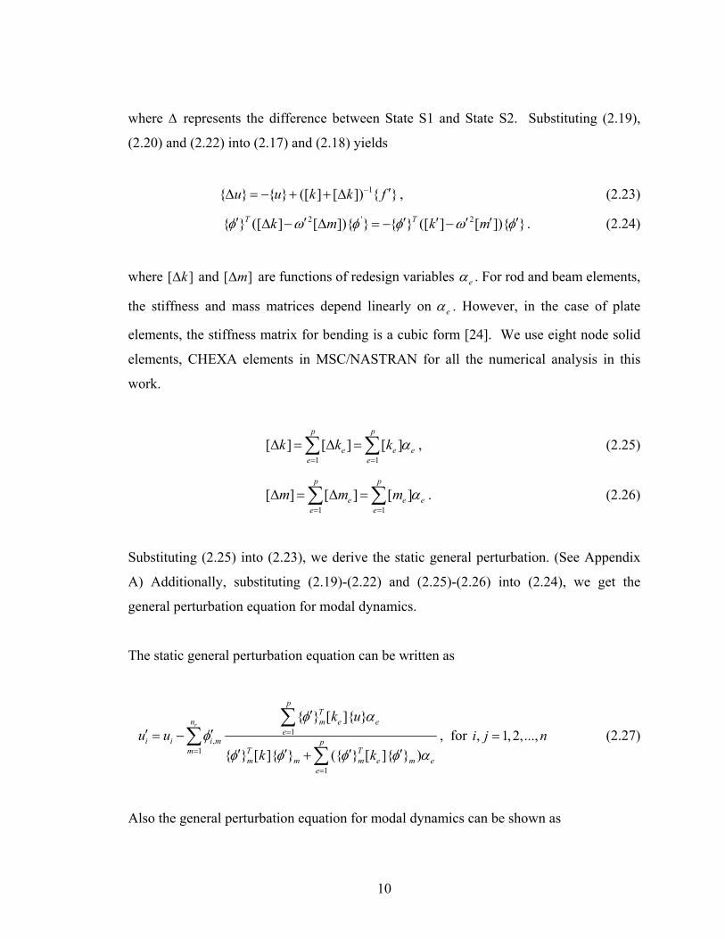
where ∆ represents the difference between State S1 and State S2. Substituting (2.19),
(2.20) and (2.22) into (2.17) and (2.18) yields
1{ } { } ([ ] [ ]) { }u u k k f− ′∆ = − + + ∆ , (2.23)
2 ' 2{ } ([ ] [ ]){ } { } ([ ] [ ]){ }T Tk m k mφ ω φ φ ω φ′ ′ ′ ′ ′ ′ ′∆ − ∆ = − − . (2.24)
where [ ]k∆ and [ ]m∆ are functions of redesign variables eα . For rod and beam elements,
the stiffness and mass matrices depend linearly on eα . However, in the case of plate
elements, the stiffness matrix for bending is a cubic form [24]. We use eight node solid
elements, CHEXA elements in MSC/NASTRAN for all the numerical analysis in this
work.
1 1[ ] [ ] [ ]
p p
e e ee e
k k k α= =
∆ = ∆ =∑ ∑ , (2.25)
1 1[ ] [ ] [ ]
p p
e e ee e
m m m α= =
∆ = ∆ =∑ ∑ . (2.26)
Substituting (2.25) into (2.23), we derive the static general perturbation. (See Appendix
A) Additionally, substituting (2.19)-(2.22) and (2.25)-(2.26) into (2.24), we get the
general perturbation equation for modal dynamics.
The static general perturbation equation can be written as
1,
1
1
{ } [ ]{ }
{ } [ ]{ } ({ } [ ]{ } )
r
pT
n m e ee
i i i m pT Tmm m m e m e
e
k uu u
k k
φ αφ
φ φ φ φ α
=
=
=
′′ ′= −
′ ′ ′ ′+
∑∑
∑, for , 1, 2,...,i j n= (2.27)
Also the general perturbation equation for modal dynamics can be shown as
11
2 2
1({ } [ ]{ } { } [ ]{ } ) { } [ ]{ } { } [ ]{ }
pT T T T Tj e i i j e i e i j i j e i
ek m m kφ φ ω φ φ α ω φ φ φ φ
=
′ ′ ′ ′ ′ ′ ′ ′ ′ ′− = −∑
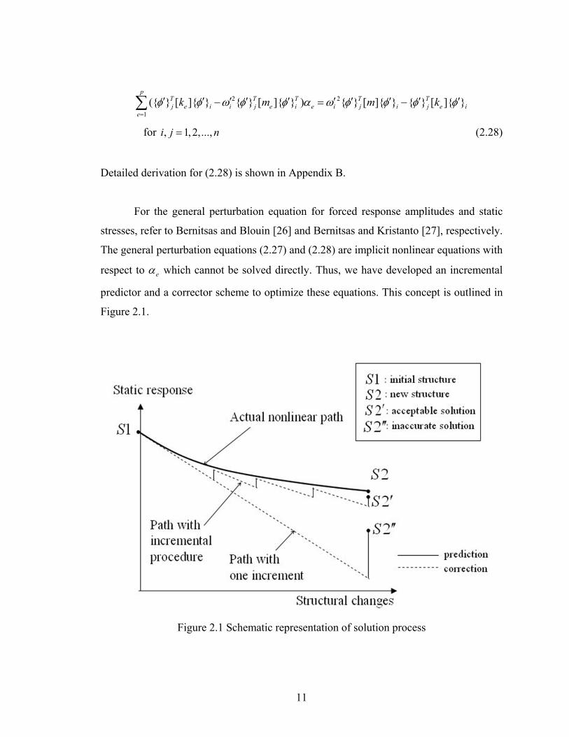
for , 1, 2,...,i j n= (2.28)
Detailed derivation for (2.28) is shown in Appendix B.
For the general perturbation equation for forced response amplitudes and static
stresses, refer to Bernitsas and Blouin [26] and Bernitsas and Kristanto [27], respectively.
The general perturbation equations (2.27) and (2.28) are implicit nonlinear equations with
respect to eα which cannot be solved directly. Thus, we have developed an incremental
predictor and a corrector scheme to optimize these equations. This concept is outlined in
Figure 2.1.
Figure 2.1 Schematic representation of solution process
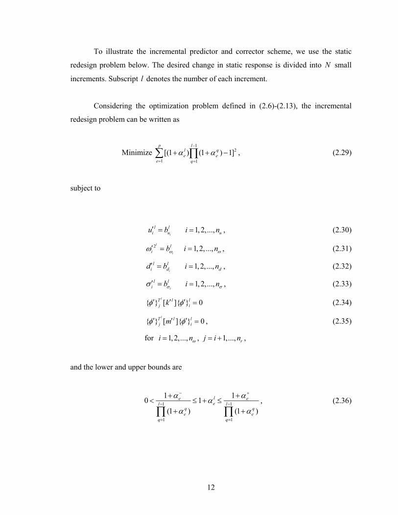
12
To illustrate the incremental predictor and corrector scheme, we use the static
redesign problem below. The desired change in static response is divided into N small
increments. Subscript l denotes the number of each increment.
Considering the optimization problem defined in (2.6)-(2.13), the incremental
redesign problem can be written as
Minimize 1
2
1 1
[(1 ) (1 ) 1]p l
l qe e
e q
α α−
= =
+ + −∑ ∏ , (2.29)
subject to
i
l li uu b′ = 1, 2,..., ui n= , (2.30)
2l
i
li bωω′ = 1, 2,...,i nω= , (2.31)
i
l li dd b′ = 1, 2,..., di n= , (2.32)
i
l li bσσ ′ = 1, 2,...,i nσ= , (2.33)
{ } [ ]{ } 0lT l l
j ikφ φ′ ′ ′ = (2.34)
{ } [ ]{ } 0lT l l
j imφ φ′ ′ ′ = , (2.35)
for 1, 2,...,i nω= , 1,..., rj i n= + ,
and the lower and upper bounds are
1 1
1 1
1 10 1(1 ) (1 )
le eel l
q qe e
q q
α ααα α
− +
− −
= =
+ +< ≤ + ≤
+ +∏ ∏, (2.36)
13
where 1
1
(1 )l
qe
q
α−
=
+∏ is known from all previous increments. For the first iteration, l is equal
to 1 by definition.
While selecting the optimal criterion as to equal the end of incremental change to
completion of the solution process, criterion (2.6) is satisfied since
1
1 (1 )N
qe e
q
α α=
+ = +∏ (2.37)
At the same time, the performance constraints satisfy the general perturbation equation
such as (2.27) and (2.28).
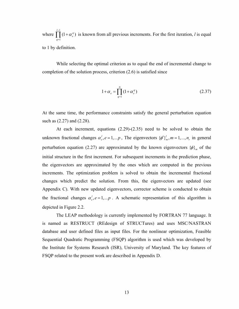
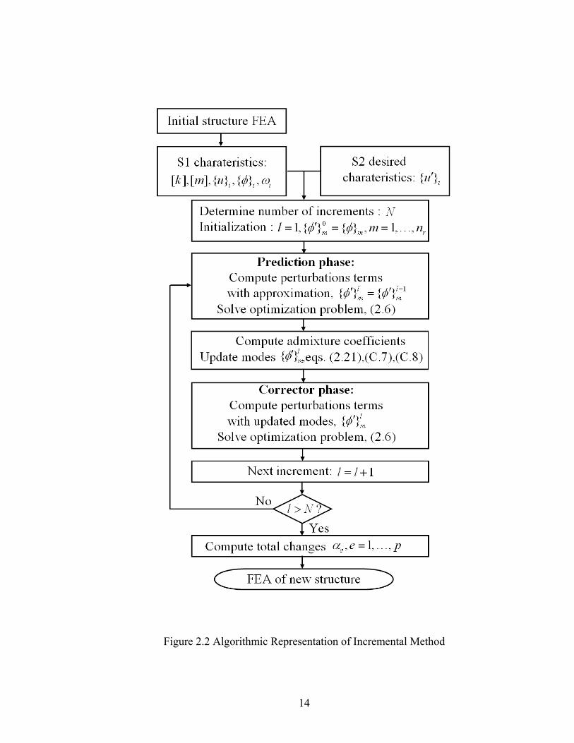
At each increment, equations (2.29)-(2.35) need to be solved to obtain the
unknown fractional changes , 1,...le e pα = , The eigenvectors { } , 1,...,l
m rm nφ′ = in general
perturbation equation (2.27) are approximated by the known eigenvectors { }mφ of the
initial structure in the first increment. For subsequent increments in the prediction phase,
the eigenvectors are approximated by the ones which are computed in the previous
increments. The optimization problem is solved to obtain the incremental fractional
changes which predict the solution. From this, the eigenvectors are updated (see
Appendix C). With new updated eigenvectors, corrector scheme is conducted to obtain
the fractional changes , 1,...le e pα = . A schematic representation of this algorithm is
depicted in Figure 2.2.
The LEAP methodology is currently implemented by FORTRAN 77 language. It
is named as RESTRUCT (REdesign of STRUCTures) and uses MSC/NASTRAN
database and user defined files as input files. For the nonlinear optimization, Feasible
Sequential Quadratic Programming (FSQP) algorithm is used which was developed by
the Institute for Systems Research (ISR), University of Maryland. The key features of
FSQP related to the present work are described in Appendix D.
14
Figure 2.2 Algorithmic Representation of Incremental Method

15
2.3. Evolutionary Structural Optimization (ESO) Algorithm
The ESO algorithm developed in this work consists of two nested loops. The
inner loop, which uses LEAP to calculate the performance equations into a form that can
be handled without trial and error or repeated FEA’s, finds incrementally the optimal
design which satisfies the objectives. The outer loop implements the search for the
optimal topology. The major characteristics of the ESO/LEAP algorithm developed in
this work are the following:
(1) The optimal topology is achieved in 3-7 iterations. In each iteration, the starting
(baseline) topology has been generated in the previous iteration. The initial topology is a
uniform, homogeneous, solid block.
(2) In the inner loop of each iteration, the LEAP algorithm is used to optimize the
structure generated by the outer loop to achieve the redesign objectives and calculate the
optimization variables eα .
(3) Following the LEAP optimization within each iteration, two heuristic criteria are used
to modify the topology in a rational way. Both address the extremes of the stiffness of the
generated elements. The first criterion eliminates elements at the lower end of the
stiffness values. The second criterion replaces high stiffness elements by the upper limit
of stiffness, which is equal to the stiffness of the available material.
In Sections 2.3.1 through 2.3.3, the heuristic criteria implemented in the topology
evolution process are presented, while in Section 2.4, the major steps of the ESO/LEAP
algorithm are described.
2.3.1. Element Elimination Criterion
To eliminate the inefficient elements, which do not contribute to the total
performance of the structure, a rejection criterion is employed. For static topology design,
the material efficiency can be measured by Static Strain Energy (SSE). Gradual removal
16
of the lower static strain energy elements leads to a more uniform distribution of material
efficiency in the evolving optimal topology compared to the initial structure. For
dynamic modal redesign, the material efficiency is measured by both the Dynamic Strain
Energy (DSE) and the Kinetic Energy (KE). Accordingly, the rejection criterion places a
lower limit on a predefined expression of the material efficiency that includes both DSE
and KE. Theoretically, the total DSE of the structure is equal to the total KE in free
vibration. The distribution of DSE, however, is different from that of KE, that is, DSE
and KE are not the same for individual elements. Thus, we need to consider both DSE
and KE in the material efficiency measure.
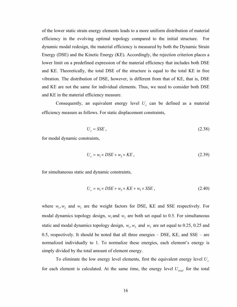
Consequently, an equivalent energy level eU can be defined as a material
efficiency measure as follows. For static displacement constraints,
eU SSE= , (2.38)
for modal dynamic constraints,
1 2eU w DSE w KE= × + × , (2.39)
for simultaneous static and dynamic constraints,
1 2 3eU w DSE w KE w SSE= × + × + × , (2.40)
where 1 2,w w and 3w are the weight factors for DSE, KE and SSE respectively. For
modal dynamics topology design, 1w and 2w are both set equal to 0.5. For simultaneous
static and modal dynamics topology design, 1 2,w w and 3w are set equal to 0.25, 0.25 and
0.5, respectively. It should be noted that all three energies – DSE, KE, and SSE – are
normalized individually to 1. To normalize these energies, each element’s energy is
simply divided by the total amount of element energy.
To eliminate the low energy level elements, first the equivalent energy level eU
for each element is calculated. At the same time, the energy level totalU for the total
17
elements in the structure is computed. All elements that satisfy the following criterion are
rejected.
e
total
U CEERU
< . (2.41)
If the element is removed, its Young’s modulus is set to a very low value close to zero
(weak material) to represent the element elimination. The elements removed virtually do
not carry any load and their energy levels are negligible. The advantage of this method is
that it does not need to regenerate a new finite element mesh at each iteration even if the
developed structure largely differs from initial structure.
Determining the value of the Cumulative Element Elimination Rate (CEER) is
explained in the next section.
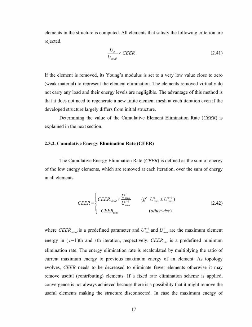
2.3.2. Cumulative Energy Elimination Rate (CEER)
The Cumulative Energy Elimination Rate (CEER) is defined as the sum of energy
of the low energy elements, which are removed at each iteration, over the sum of energy
in all elements.
1maxmax max1
max
min
( )
( )
ii i
initial i
UCEER if U UCEER U
CEER otherwise
−−
⎧× ≤⎪= ⎨
⎪⎩
(2.42)
where initialCEER is a predefined parameter and 1maxiU − and max
iU are the maximum element
energy in ( 1i − )th and i th iteration, respectively. minCEER is a predefined minimum
elimination rate. The energy elimination rate is recalculated by multiplying the ratio of
current maximum energy to previous maximum energy of an element. As topology
evolves, CEER needs to be decreased to eliminate fewer elements otherwise it may
remove useful (contributing) elements. If a fixed rate elimination scheme is applied,
convergence is not always achieved because there is a possibility that it might remove the
useful elements making the structure disconnected. In case the maximum energy of
18
current iteration exceeds the previous iteration, we assign the CEER a minimum
elimination rate, which is a very small value between 0.001 and 0.015. At this stage,
minimum elimination rate should be applied since every remaining element carries
concentrated energy. Under this condition, the total energy distribution is approaching
convergence level and therefore minCEER should be used.
2.3.3. Element Freezing Criterion
Following elimination of the low efficiency elements based on the CEER criterion,
the element freezing criterion is used to manage the other extreme of Young’s modulus.
Specifically, elements with values of Young’s modulus greater than sE are assigned a
value of Young’s modulus equal to sE , which is defined by the designer. This process,
on one hand, makes the material more uniform and on the other hand, places an upper
limit on the extreme values of Young’s modulus generated in the redesign process.
Accordingly, the optimal material distribution produced by RESTRUCT is adjusted
based on the following criterion
1 ,,
sie i
e
EE
E+ ⎧= ⎨⎩
ie sie s
E EE E
≥<
(2.43)
where 1ieE + is the Young’s modulus of element e for the next iteration. i
eE is the current
element material property in RESTRUCT. When the material property of an element
reaches sE , it is frozen at the material value of sE In the rest of the optimization process,
only the elements that have not been eliminated or have not been frozen are used.
2.4. Optimization Process Steps
There are two loops in the optimization process. The outer loop sets the updated
topology based on the two heuristic criteria defined above. The inner loop optimizes the

19
redesign variables to achieve the performance objectives. The major steps of the
ESO/LEAP algorithm are shown schematically in Figure 2.3.

20
Figure 2.3 Algorithmic Representation of ESO/LEAP (Evolutionary Structural Optimization / LargE Admissible Perturbation) methodology
21
For the inner loop, RESTRUCT process is used to find the structural changes, eα
by incremental predictor-corrector scheme which is explained in Section 2.2. If the
calculated results satisfy the performance goals, it continues to the next step. The element
elimination is applied with Cumulative Energy Elimination Rate (CEER) and freezing
criteria. Then Young’s modulus values of all elements which are not eliminated and
Young’s modulus value is below sE , are set to sE temporarily. This process is to check
whether the structure with Young’s modulus properties of the elements are all equal to
sE satisfies the performance criteria or not. If it satisfies the criteria, stop the
optimization process and converged result is obtained.
The optimization criteria for the outer loop are the norm between desired
performance objective and calculated performance values. It can be written as
s s ε′ − < (2.44)
where s′ is designer specified performance objectives and s is calculated performance
values. If the absolute value of difference is less than ε , optimization process is
terminated and we get a new objective structure. 5% is used as the criteria value for this
work. If the criterion is not satisfied, it returns to the beginning of the RESTRUCT
process as depicted in Figure 2.3.

22
CHAPTER III
PARAMETRIC EVOLUTION RESULTS
In this Chapter, two numerical applications are presented in static, dynamic, and
simultaneous (static and dynamic) redesign. The first application is a cantilever beam
with a concentrated force applied at the free-end as shown in Figure 3.1. The design
domain has length 16 mm, height 10 mm and thickness 3 mm. Initial Young’s modulus
is 50 2.07 10E MPa= × , Poisson’s ratio 0.3ν = , and mass density
9 2 47.833 10 /Ns mmρ −= × . A 300N force is applied downward at the center of the free-
end. A finite element mesh of 32×20 is used.
Figure 3.1. Cantilever beam with one point load at the center of the free-end
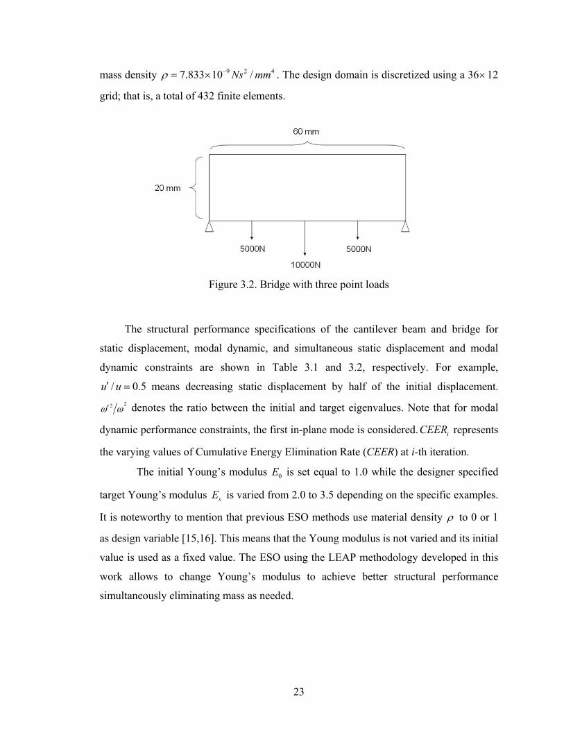
The second example is a simply supported bridge with three point forces [5]. Loads
are applied to the bottom of the initial structure. It has a 60 mm×20 mm domain with 1
mm thickness. Initial Young’s modulus 50 2.07 10E MPa= × , Poisson’s ratio 0.3ν = , and
23
mass density 9 2 47.833 10 /Ns mmρ −= × . The design domain is discretized using a 36×12
grid; that is, a total of 432 finite elements.
Figure 3.2. Bridge with three point loads
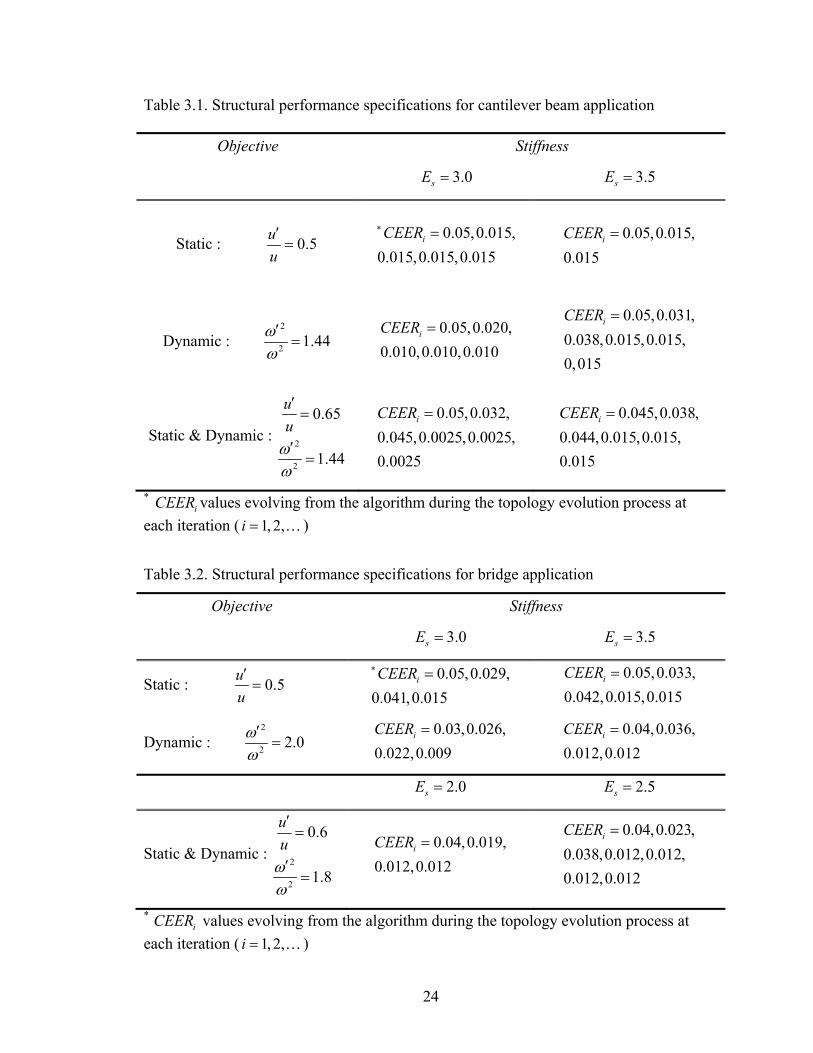
The structural performance specifications of the cantilever beam and bridge for
static displacement, modal dynamic, and simultaneous static displacement and modal
dynamic constraints are shown in Table 3.1 and 3.2, respectively. For example,
/ 0.5u u′ = means decreasing static displacement by half of the initial displacement. 22ω ω′ denotes the ratio between the initial and target eigenvalues. Note that for modal
dynamic performance constraints, the first in-plane mode is considered. iCEER represents
the varying values of Cumulative Energy Elimination Rate (CEER) at i-th iteration.
The initial Young’s modulus 0E is set equal to 1.0 while the designer specified
target Young’s modulus sE is varied from 2.0 to 3.5 depending on the specific examples.
It is noteworthy to mention that previous ESO methods use material density ρ to 0 or 1
as design variable [15,16]. This means that the Young modulus is not varied and its initial
value is used as a fixed value. The ESO using the LEAP methodology developed in this
work allows to change Young’s modulus to achieve better structural performance
simultaneously eliminating mass as needed.
24
Table 3.1. Structural performance specifications for cantilever beam application
Objective Stiffness
3.0sE = 3.5sE =
Static : 0.5uu′=
0.05,0.015,0.015,0.015,0.015
iCEER∗ = 0.05,0.015,0.015
iCEER =
Dynamic : 2
2 1.44ωω′=
0.05,0.020,0.010,0.010,0.010
iCEER =
0.05,0.031,0.038,0.015,0.015,0,015
iCEER =
Static & Dynamic : 2
2
0.65
1.44
uuωω
′=
′=
0.05,0.032,
0.045,0.0025,0.0025,0.0025
iCEER =
0.045,0.038,0.044,0.015,0.015,0.015
iCEER =
* iCEER values evolving from the algorithm during the topology evolution process at each iteration ( 1, 2,i = … )
Table 3.2. Structural performance specifications for bridge application
Objective Stiffness
3.0sE = 3.5sE =
Static : 0.5uu′=
0.05,0.029,0.041,0.015
iCEER∗ = 0.05,0.033,
0.042,0.015,0.015iCEER =
Dynamic : 2
2 2.0ωω′=
0.03,0.026,0.022,0.009
iCEER =
0.04,0.036,0.012,0.012
iCEER =
2.0sE = 2.5sE =
Static & Dynamic : 2
2
0.6
1.8
uuωω
′=
′=
0.04,0.019,
0.012,0.012iCEER =
0.04,0.023,
0.038,0.012,0.012,0.012,0.012
iCEER =
* iCEER values evolving from the algorithm during the topology evolution process at
each iteration ( 1, 2,i = … )
25
3.1. Static Displacement Problem
As shown in Table 3.1 and Table 3.2, the static displacement objective is to
decrease the displacement at the loading point by a factor of 2. It is tested using two
target values for sE , 3.0 and 3.5. That is, the element Young’s modulus starts from initial
value 0E =1.0 and increased up to the target sE value of 3.0 or 3.5. The initial CEER
value is set at 0.05.
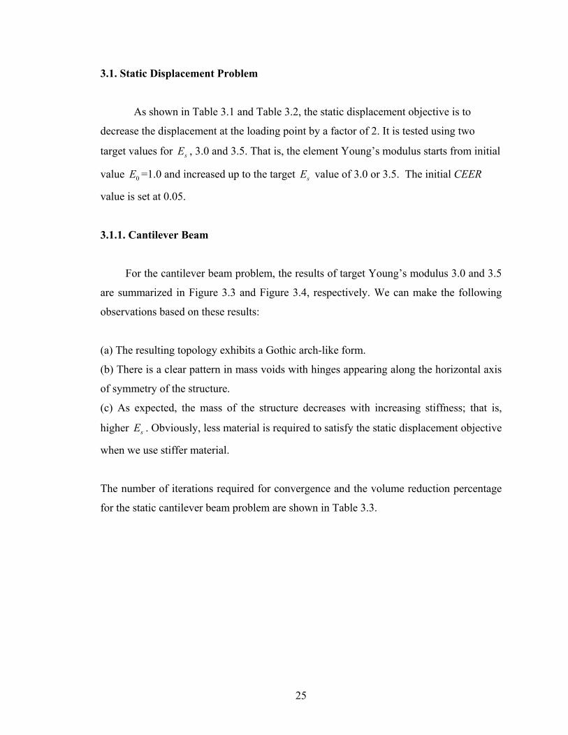
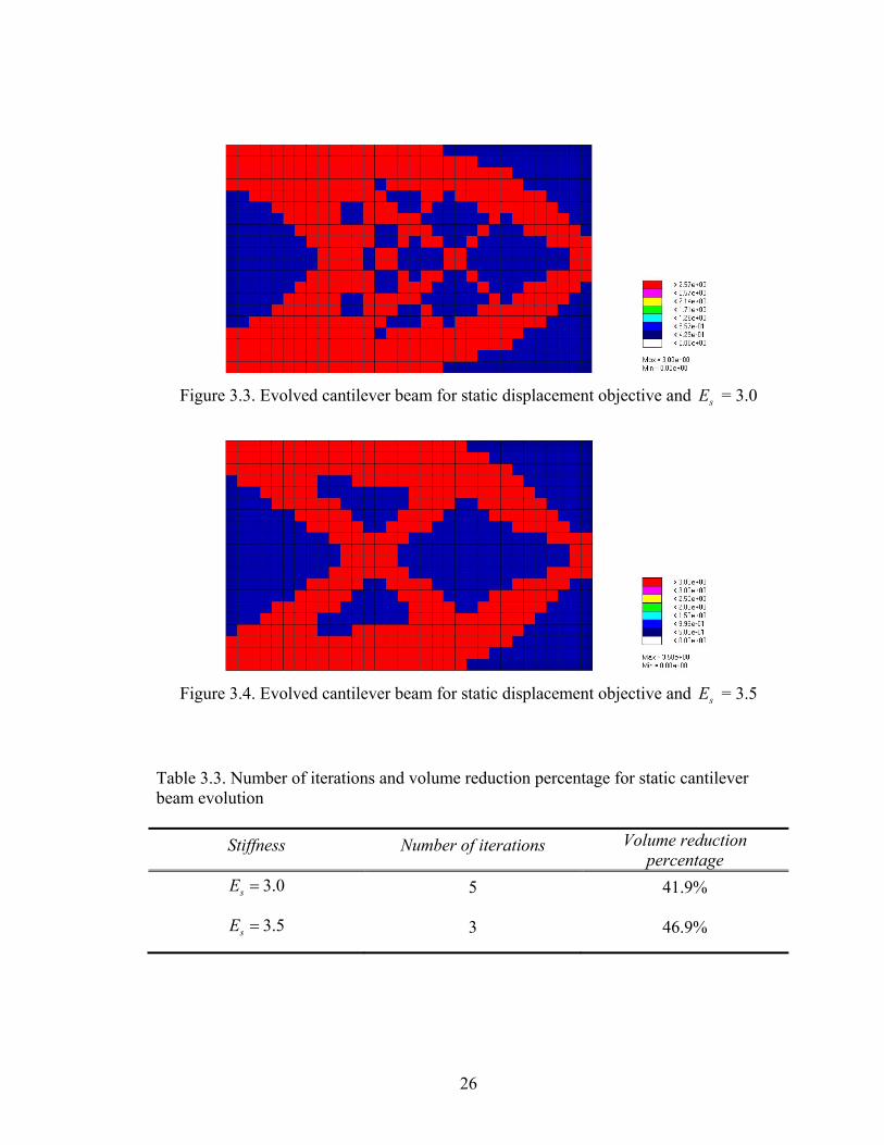
3.1.1. Cantilever Beam
For the cantilever beam problem, the results of target Young’s modulus 3.0 and 3.5
are summarized in Figure 3.3 and Figure 3.4, respectively. We can make the following
observations based on these results:
(a) The resulting topology exhibits a Gothic arch-like form.
(b) There is a clear pattern in mass voids with hinges appearing along the horizontal axis
of symmetry of the structure.
(c) As expected, the mass of the structure decreases with increasing stiffness; that is,
higher sE . Obviously, less material is required to satisfy the static displacement objective
when we use stiffer material.
The number of iterations required for convergence and the volume reduction percentage
for the static cantilever beam problem are shown in Table 3.3.
26
Figure 3.3. Evolved cantilever beam for static displacement objective and sE = 3.0
Figure 3.4. Evolved cantilever beam for static displacement objective and sE = 3.5
Table 3.3. Number of iterations and volume reduction percentage for static cantilever beam evolution
Stiffness Number of iterations Volume reduction percentage
3.0sE = 5 41.9%
3.5sE = 3 46.9%

27
Comparing present work to the recently developed Bi-directional Evolutionary
Structural Optimization (BESO) method, the ESO/LEAP achieves very similar topology
only in three iterations while the BESO methodology requires at least 70 iterations [15].
Further, the BESO method, when the volume reaches its objective value, which is 50% of
the total design domain, the mean compliance converges to a constant value of 1.87 Nmm.
The present method achieves volume reduction of 46.9% and mean compliance of 1.60
Nmm with significantly decreased number of iterations.
3.1.2. Bridge
The objective of the bridge example is to reduce static displacement by half at mid-
span of the bridge bottom, where the largest force is applied. The converged results are
shown in Figure 3.5 and Figure 3.6 using two different sE values of 3.0 and 3.5,
respectively. The number of iterations and volume reduction percentages are listed in
Table 3.4. The resulting topology exhibits the following features:
(a) Curved and straight elements evolved from the initial solid structure to form a bridge-
like structure to support the three point loads while observing the two fixed boundary
points.
(b) Using higher sE , i.e., stiffer material, requires less material to achieve the specified
performance.
(c) There is similarity in voids and joints between the two cases. In the less stiff material
case, more material is required to support the applied loads. As expected, the higher
Young’s modulus structure develops thinner members than the less stiff material case.
(d) The lack of bridge bottom can be justified intuitively. Loads are not applied along the
entire bottom of the bridge. Accordingly, the three vertical structural members evolve
which transfer the bottom loads to the arch above which is a most efficient way of
supporting loads between two boundaries.

28
Figure 3.5. Evolved bridge for static displacement objective and sE = 3.0
Figure 3.6. Evolved bridge for static displacement objective and sE = 3.5
Table 3.4. Number of iterations and volume reduction percentage for static bridge evolution
Stiffness Number of iterations Volume reduction
percentage
3.0sE = 4 45.4%
3.5sE = 5 54.6%
29
3.2. Modal Dynamic Problem
The modal dynamic problem is to increase the first eigenvalue corresponding to the
in-plane bending mode. For the cantilever beam, the objective is to increase the first
eigenvalue by a factor of 1.44. For the bridge, the objective is to increase the first
eigenvalue by a factor of 2.0.
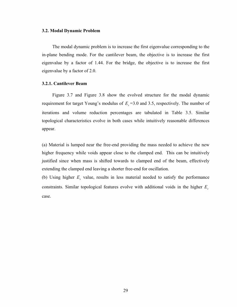
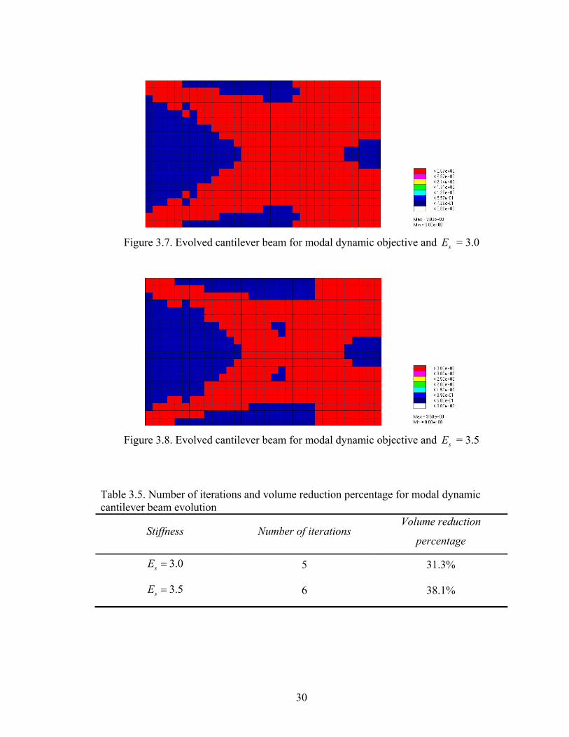
3.2.1. Cantilever Beam
Figure 3.7 and Figure 3.8 show the evolved structure for the modal dynamic
requirement for target Young’s modulus of sE =3.0 and 3.5, respectively. The number of
iterations and volume reduction percentages are tabulated in Table 3.5. Similar
topological characteristics evolve in both cases while intuitively reasonable differences
appear.
(a) Material is lumped near the free-end providing the mass needed to achieve the new
higher frequency while voids appear close to the clamped end. This can be intuitively
justified since when mass is shifted towards to clamped end of the beam, effectively
extending the clamped end leaving a shorter free-end for oscillation.
(b) Using higher sE value, results in less material needed to satisfy the performance
constraints. Similar topological features evolve with additional voids in the higher sE
case.
30
Figure 3.7. Evolved cantilever beam for modal dynamic objective and sE = 3.0
Figure 3.8. Evolved cantilever beam for modal dynamic objective and sE = 3.5
Table 3.5. Number of iterations and volume reduction percentage for modal dynamic cantilever beam evolution
Stiffness Number of iterations Volume reduction
percentage
3.0sE = 5 31.3%
3.5sE = 6 38.1%

31
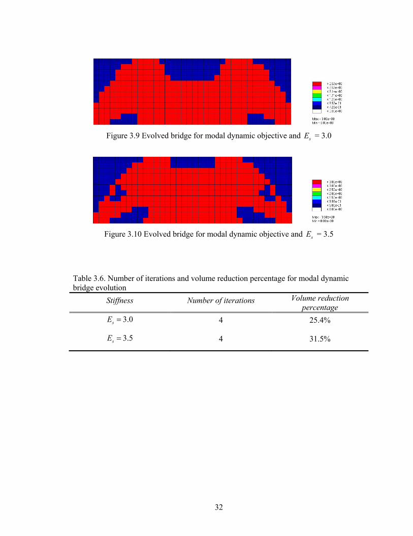
3.2.2. Bridge
For the bridge topology evolution examples, the modal dynamic performance
objective is to increase the first eigenvalue of the in-plane bending mode by a factor of
2.0. The results are shown in Figure 3.9 and Figure 3.10. using sE =3.0 and 3.5,
respectively. The following observations can be made:
(a) For both cases, the mass is preserved in the middle of the structure where the
amplitude of oscillation is higher.
(b) Higher target Young’s modulus sE results in voids near the end supports – away from
the high oscillations at the center of the bridge. This decreases the total volume. The
modal dynamic requirement is still satisfied in spite of the reduced stiffness. The higher
sE compensates for loss of stiffness.
32
Figure 3.9 Evolved bridge for modal dynamic objective and sE = 3.0
Figure 3.10 Evolved bridge for modal dynamic objective and sE = 3.5
Table 3.6. Number of iterations and volume reduction percentage for modal dynamic bridge evolution
Stiffness Number of iterations Volume reduction percentage
3.0sE = 4 25.4%
3.5sE = 4 31.5%
33
3.3. Simultaneous Static and Modal Dynamic Problem
In this section, static displacement and modal dynamic performance objectives are
considered at the same time. As shown in Table 3.1, the objectives for the cantilever
beam topology evolution are to reduce the displacement of a specific point by a factor of
0.65 for the cantilever beam and to increase the first eigenvalue of the in-plane bending
mode by a factor of 1.44. For the bridge example, the objective for static displacement is
to reduce the amplitude by a factor of 0.6 and simultaneously to increase the first
eigenvalue by a factor of 1.8. The initial Cumulative Energy Elimination Rate (CEER) is
0.045 for cantilever beam and 0.04 for the bridge example.
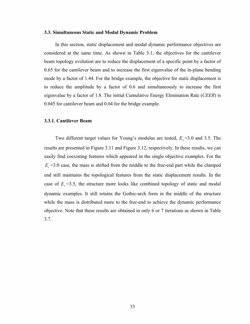
3.3.1. Cantilever Beam
Two different target values for Young’s modulus are tested, sE =3.0 and 3.5. The
results are presented in Figure 3.11 and Figure 3.12, respectively. In these results, we can
easily find coexisting features which appeared in the single objective examples. For the
sE =3.0 case, the mass is shifted from the middle to the free-end part while the clamped
end still maintains the topological features from the static displacement results. In the
case of sE =3.5, the structure more looks like combined topology of static and modal
dynamic examples. It still retains the Gothic-arch form in the middle of the structure
while the mass is distributed more to the free-end to achieve the dynamic performance
objective. Note that these results are obtained in only 6 or 7 iterations as shown in Table
3.7.
34
Figure 3.11. Evolved cantilever beam for static displacement/modal
dynamic objective and sE = 3.0
Figure 3.12. Evolved cantilever beam for static displacement/modal
dynamic objective and sE = 3.5 Table 3.7. Number of iterations and volume reduction percentage for static displacement and modal dynamic of cantilever beam evolution
Stiffness Number of iterations Volume reduction percentage
3.0sE = 6 42.5%
3.5sE = 7 44.4%

35
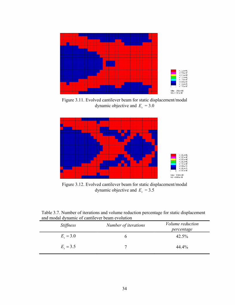
3.3.2. Bridge
In this example, target Young’s modulus values of sE =2.0 and 2.5 are used. The
converged results are shown in Figure 3.13 and Figure 3.14. These results show
simultaneous characteristics observed in the static displacement and modal dynamic cases
independently. The following observations are made:
(a) The overall arch shape which evolved in the static displacement case is still
predominant.
(b) Mass is lumped near the center where maximum oscillation occurs.
(c) The three voids observed in the static displacement evolution are still present in the
middle. The size of the voids, however, is decreased.
36
Figure 3.13. Evolved bridge for static displacement/modal
dynamic objective and sE = 2.0
Figure 3.14. Evolved bridge for static displacement/modal
dynamic objective and sE = 2.5 Table 3.8. Number of iterations and volume reduction percentage for static displacement and modal dynamic bridge evolution
Stiffness Number of iterations Volume reduction
percentage
2.0sE = 4 25.9%
2.5sE = 6 38.4%

37
The advantage of applying the Cumulative Energy Elimination Rate (CEER)
scheme instead of fixed rate elimination method [30], the converged result is obtained
much faster. For example, it requires 6 or 10 iterations to get the similar converging
results in static problem 3.5sE = while it takes only 3 iterations. All the other examples
in the present work show less or same number of iterations.
Additionally, since fixed elimination rate method removes constant number of
elements at each iteration, it sometimes eliminates useful elements which are critical to
structural stability. The CEER scheme can overcome this problem by removing very
small portion of the elements when the optimization process is close to convergence.

38
3.4. Topology Evolution with Increased Resolution
In this section, the cantilever example with increased resolution of the finite
element mesh is tested. A finite element mesh of 48 × 30 is used. The performance
constraints applied are same as shown in Table 3.1. Only the static displacement and
modal dynamic constraints are applied separately. The designer specified target Young’s
modulus sE is set equal to 3.0.
Evolved cantilever beam for static displacement and modal dynamic objective are
exhibited in Figure 3.15 and Figure 3.16, respectively. Comparing these results to the
32 × 20 mesh results, which are shown in Figure 3.3 and Figure 3.7, very similar
characteristics can be observed. The topological features are similar in both applications
with nearly the same volume reduction achieved. As shown in Table 3.9, it only takes 6
iterations in both cases to obtain the converged results in spite of the increased resolution
of the finite element mesh used.

39
Figure 3.15. Evolved cantilever beam for static displacement objective
with high resolution
Figure 3.16. Evolved cantilever beam for modal dynamic objective
with high resolution
Table 3.9. Number of iterations and volume reduction for the high resolution cantilever beam evolution
Objective Number of iterations Volume reduction
percentage
Static: 0.5uu′= 6 39.9%
Modal dynamic : 2
2 1.44ωω′= 6 33.7%
40
3.5. Topology Evolution with Performance Constraints Varied
Most of the topology optimization methods in the literature impose a volume
constraint [3,7,15,16] while achieving maximum stiffness (i.e., compliance minimization).
The ESO/LEAP algorithm developed in this work has no volume constraint since there is
no limit or stopping criterion for volume reduction.
In this section, the topology evolution results using the ESO/LEAP methodology
with applying different values of structural performance constraints are presented. The
results show that the volume resulting in the final structure can be adjusted by applying
different performance constraint values.
3.5.1. Static Displacement Constraints
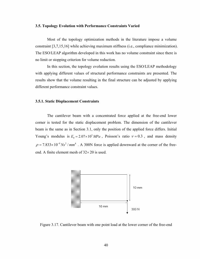
The cantilever beam with a concentrated force applied at the free-end lower
corner is tested for the static displacement problem. The dimension of the cantilever
beam is the same as in Section 3.1, only the position of the applied force differs. Initial
Young’s modulus is 50 2.07 10E MPa= × , Poisson’s ratio 0.3ν = , and mass density
9 2 47.833 10 /Ns mmρ −= × . A 300N force is applied downward at the corner of the free-
end. A finite element mesh of 32×20 is used.
Figure 3.17. Cantilever beam with one point load at the lower corner of the free-end

41
The static displacement objective is to change the displacement at the loading
point by a factor of 0.5, 0.65 and 0.8. The results are shown in Figure 3.18, Figure 3.19,
and Figure 3.20, respectively.

42
Figure 3.18. Evolved cantilever beam with lower corner force for static displacement
objective / 0.5u u′ =
Figure 3.19. Evolved cantilever beam with lower corner force for static displacement
objective / 0.65u u′ =
Figure 3.20. Evolved cantilever beam with lower corner force for static displacement
objective / 0.8u u′ =
43
Table 3.10. Number of iterations and volume reduction for static displacement objective of cantilever beam evolution with lower corner force
Objective Number of iterations Volume reduction
percentage
Static: 0.5uu′= 4 44.8%
Static: 0.65uu′= 4 51.9%
Static: 0.8uu′= 5 68.0%
We can make the following observations:
(a) By increasing the ratio of static deflection, the volume reduction rate of the objective
structure increases. As expected, less material is required to design a more flexible
structure.
(b) The topological branches evolve to a simple and thinner form when the static
displacement constraint is more flexible.
(c) Obviously, the volume result can be adjusted by changing the value of the static
displacement constraint.
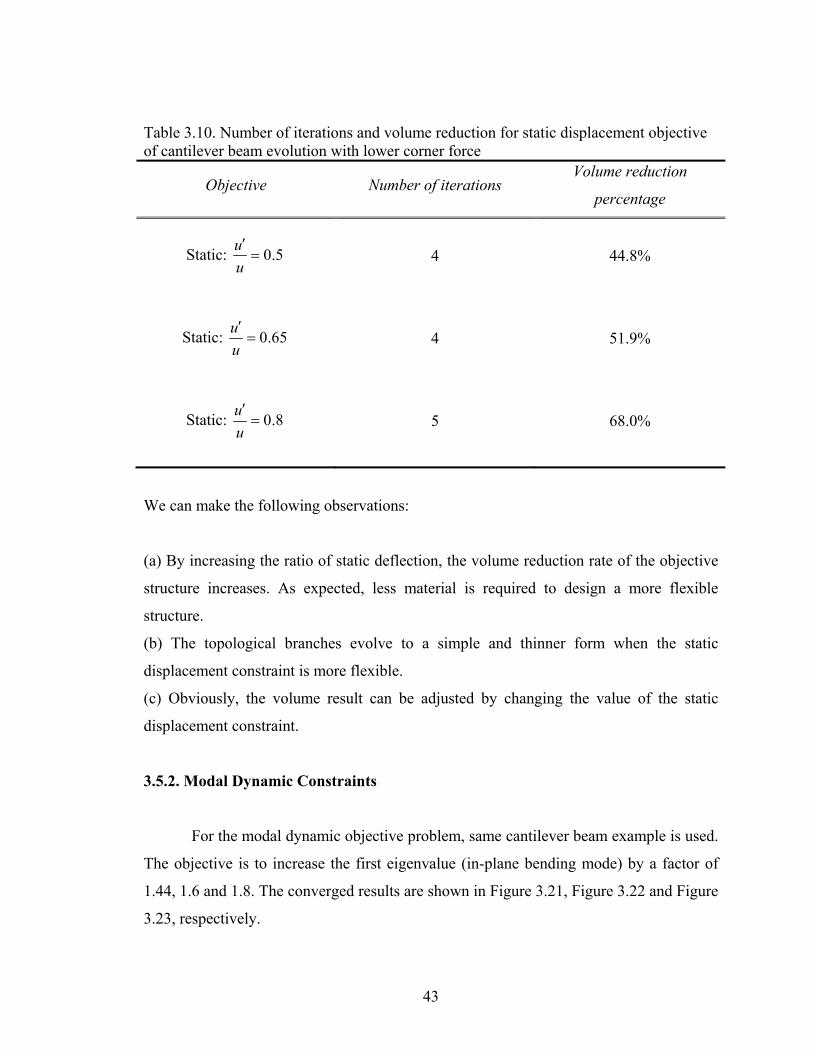
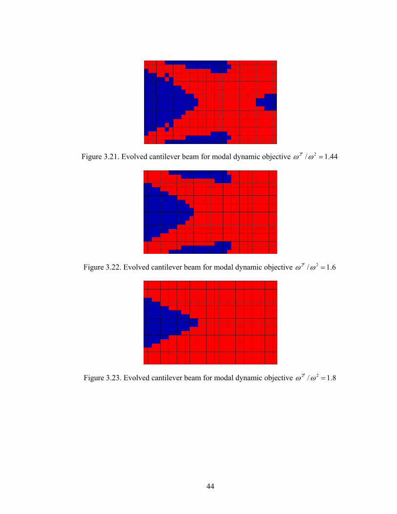
3.5.2. Modal Dynamic Constraints
For the modal dynamic objective problem, same cantilever beam example is used.
The objective is to increase the first eigenvalue (in-plane bending mode) by a factor of
1.44, 1.6 and 1.8. The converged results are shown in Figure 3.21, Figure 3.22 and Figure
3.23, respectively.
44
Figure 3.21. Evolved cantilever beam for modal dynamic objective 2 2/ 1.44ω ω′ =
Figure 3.22. Evolved cantilever beam for modal dynamic objective 2 2/ 1.6ω ω′ =
Figure 3.23. Evolved cantilever beam for modal dynamic objective 2 2/ 1.8ω ω′ =

45
Table 3.11. Number of iterations and volume reduction for modal dynamic objective of cantilever beam evolution
Objective Number of iterations Volume reduction
percentage
Modal dynamic : 2
2 1.44ωω′= 5 31.3%
Modal dynamic : 2
2 1.6ωω′= 3 25.9%
Modal dynamic : 2
2 1.8ωω′= 2 14.0%
As shown in Table 3.11, more mass remains with increasing factor of modal
dynamic constraints. Intuitively, the mass should be reduced more to increase the in-
plane bending mode since the eigenvalue is proportional to square root of stiffness over
mass. However, the results indicate that the stiffness of the structure increases faster then
the mass in the optimization process, less material is needed with increased value of the
modal dynamic constraint.

46
CHAPTER IV
TOPOLOGY EVOLUTION PATTERNS
In this Chapter, topology evolution patterns for the examples are presented in
Chapter III. Results clearly show that topological patterns develop at each iteration until
convergence, while element energy is concentrated to remaining elements.
4.1. Static Displacement Topology Evolution Patterns
The static displacement topology evolution patterns are shown in this section.
The objective is to decrease the displacement at the loading point by a factor of 2. It is
tested using two values for sE , 3.0 and 3.5.
4.1.1. Cantilever Beam
For the cantilever beam, the results of topology evolution are shown in Figure 4.1
and Figure 4.2 using target Young’s modulus 3.0 and 3.5, respectively. Based on these
results, we can make the following observations:
(a) First, the edges including the corners at which the fixed boundary condition is applied,
reach the target Young’s modulus (i.e., therefore freeze first). Then, element freezing
propagates into the middle of the structure as the structure develops.
(b) The Gothic arch-like form appears first and then detailed shapes such as holes and
branches are developed.
(c) The number of holes increases as the structure evolves toward the optimal topology.

47
(a) Iteration 1
(b) Iteration 2
(c) Iteration 3

48
(d) Iteration 4
(e) Iteration 5
Figure 4.1. Topology evolution pattern for cantilever beam - static displacement objective and sE =3.0

49
(a) Iteration 1
(b) Iteration 2
(c) Iteration 3
Figure 4.2. Topology evolution pattern for cantilever beam - static displacement objective and sE =3.5

50
4.1.2. Bridge
The objective of the bridge example is to reduce the static displacement by half at
mid-span of the bridge bottom, where the largest force is applied and the largest
displacement occurs. The results of the topology evolution are shown in Figure 4.3 and
Figure 4.4 using sE values of 3.0 and 3.5, respectively.
(a) The simply supported ends and the top part of the bridge reach the target Young’s
modulus first.
(b) Three vertical structural members appear clearly as the topology evolution proceeds
in both cases. These two cases show development of similar topological features, but in
the stiffer material case, less material is required to support the given loads thus making
the size of the voids and holes larger.
(c) The hole in the middle of the bridge emerges in the later stage of the evolving process.

51
(a) Iteration 1
(b) Iteration 2
(c) Iteration 3
(d) Iteration 4
Figure 4.3. Topology evolution pattern for bridge - static displacement objective and sE =3.0

52
(a) Iteration 1
(b) Iteration 2
(c) Iteration 3

53
(d) Iteration 4
(e) Iteration 5
Figure 4.4. Topology evolution pattern for bridge - static displacement objective and sE =3.5

54
4.2. Modal Dynamic Topology Evolution Patterns
The objective of modal dynamic example is to increase the first eigenvalue which
corresponds to the in-plane bending. For the cantilever beam, the objective is to increase
by the factor of 1.44 and for the bridge the objective is to increase by a factor of 2.0.
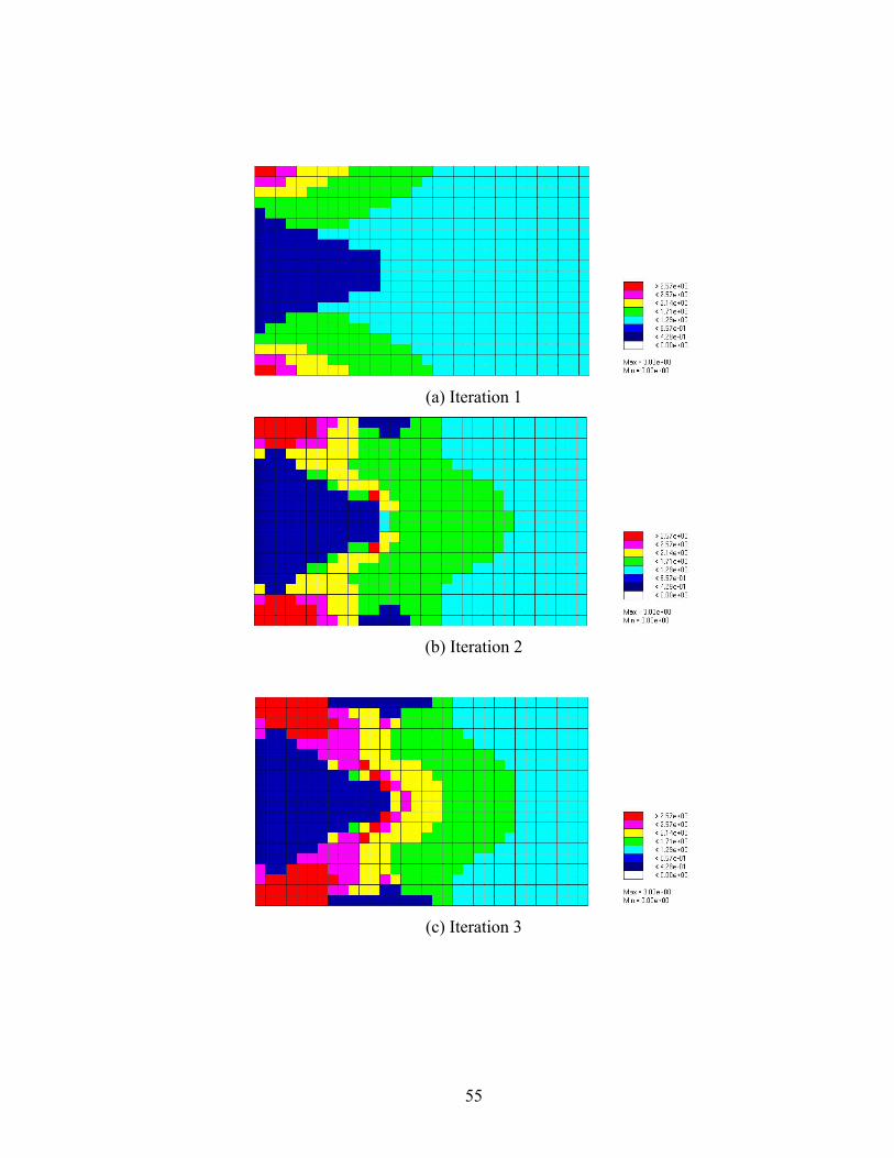
4.2.1. Cantilever Beam
Figure 4.5 and Figure 4.6 show the topology evolution for the modal dynamic
constraints using different target Young’s modulus sE of 3.0 and 3.5, respectively. The
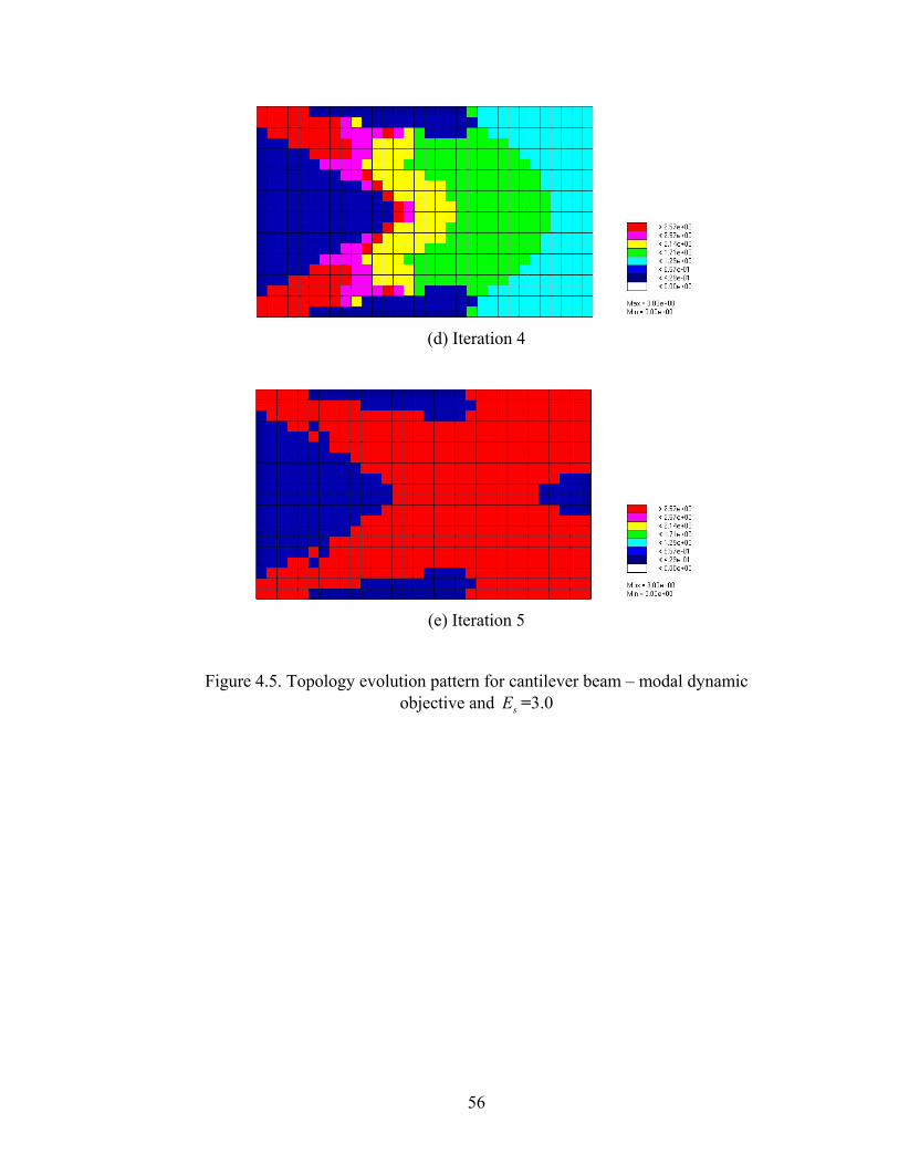
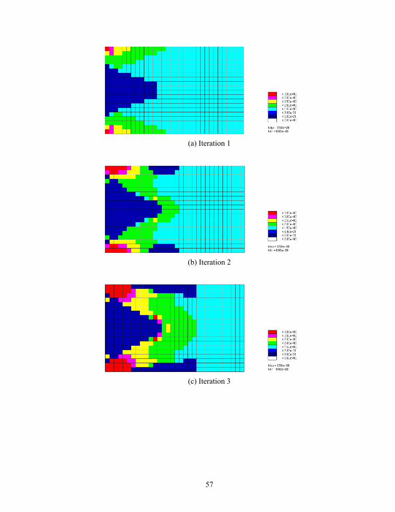
resulting topology exhibits the following features:
(a) At first, the clamped corners of the left side of the structure reach the target Young’s
modulus. Then, the remaining elements are frozen in the middle of the structure as the
structure evolves to the objective design.
(b) The material near the free-end almost remains intact during the evolution process.
This provides the mass needed to achieve modal dynamic goals while voids appear close
to the clamped end.
(c) Both cases sE of 3.0 and 3.5 exhibits very similar topological development process,
while using higher sE value results in two small holes in the center of the structure in the
later stage of the evolution.
55
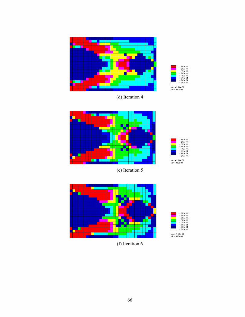
(a) Iteration 1
(b) Iteration 2
(c) Iteration 3
56
(d) Iteration 4
(e) Iteration 5
Figure 4.5. Topology evolution pattern for cantilever beam – modal dynamic objective and sE =3.0
57
(a) Iteration 1
(b) Iteration 2
(c) Iteration 3
58
(d) Iteration 4
(e) Iteration 5
(f) Iteration 6
Figure 4.6. Topology evolution pattern for cantilever beam – modal dynamic objective and sE =3.5
59
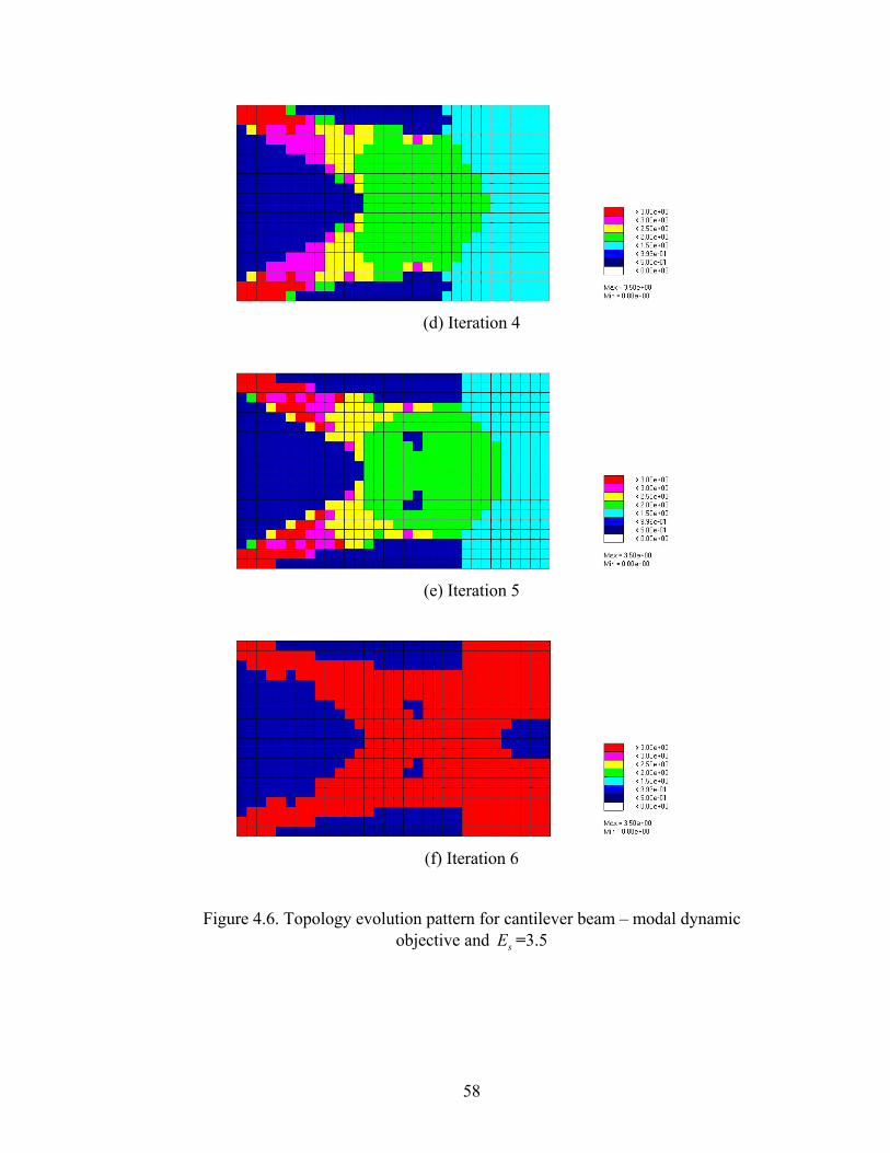
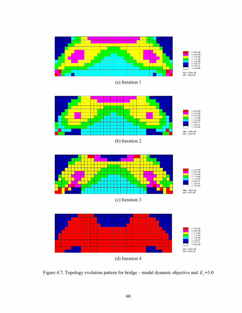
4.2.2. Bridge
For the bridge example, the modal dynamic objective is to increase the first
eigenvalue by a factor of 2.0. The results of topology evolution are depicted in Figure 4.7
and Figure 4.8. The resulting topology exhibits the following features.
(a) For both cases, the mass is preserved in the middle of the structure throughout the
evolution process.
(b) The topological evolution is similar for both cases. However, the holes near the end
supports appear in the last iteration for the higher target Young’s modulus sE case.
60
(a) Iteration 1
(b) Iteration 2
(c) Iteration 3
(d) Iteration 4
Figure 4.7. Topology evolution pattern for bridge – modal dynamic objective and sE =3.0

61
(a) Iteration 1
(b) Iteration 2
(c) Iteration 3
(d) Iteration 4
Figure 4.8. Topology evolution pattern for bridge – modal dynamic objective and sE =3.5
62
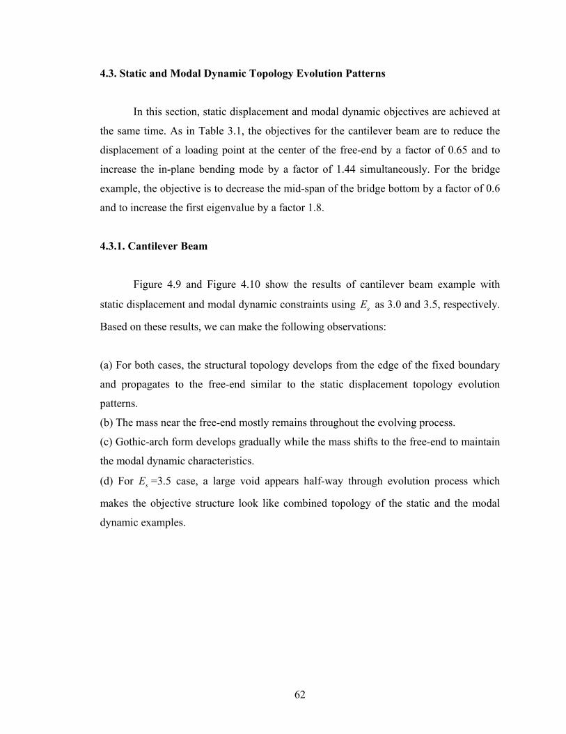
4.3. Static and Modal Dynamic Topology Evolution Patterns
In this section, static displacement and modal dynamic objectives are achieved at
the same time. As in Table 3.1, the objectives for the cantilever beam are to reduce the
displacement of a loading point at the center of the free-end by a factor of 0.65 and to
increase the in-plane bending mode by a factor of 1.44 simultaneously. For the bridge
example, the objective is to decrease the mid-span of the bridge bottom by a factor of 0.6
and to increase the first eigenvalue by a factor 1.8.
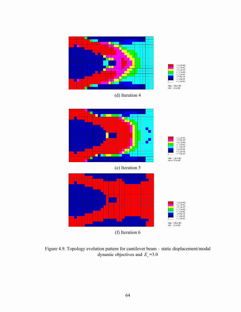
4.3.1. Cantilever Beam
Figure 4.9 and Figure 4.10 show the results of cantilever beam example with
static displacement and modal dynamic constraints using sE as 3.0 and 3.5, respectively.
Based on these results, we can make the following observations:
(a) For both cases, the structural topology develops from the edge of the fixed boundary
and propagates to the free-end similar to the static displacement topology evolution
patterns.
(b) The mass near the free-end mostly remains throughout the evolving process.
(c) Gothic-arch form develops gradually while the mass shifts to the free-end to maintain
the modal dynamic characteristics.
(d) For sE =3.5 case, a large void appears half-way through evolution process which
makes the objective structure look like combined topology of the static and the modal
dynamic examples.

63
(a) Iteration 1
(b) Iteration 2
(c) Iteration 3
64
(d) Iteration 4
(e) Iteration 5
(f) Iteration 6
Figure 4.9. Topology evolution pattern for cantilever beam – static displacement/modal dynamic objectives and sE =3.0
65
(a) Iteration 1
(b) Iteration 2
(c) Iteration 3
66
(d) Iteration 4
(e) Iteration 5
(f) Iteration 6
67
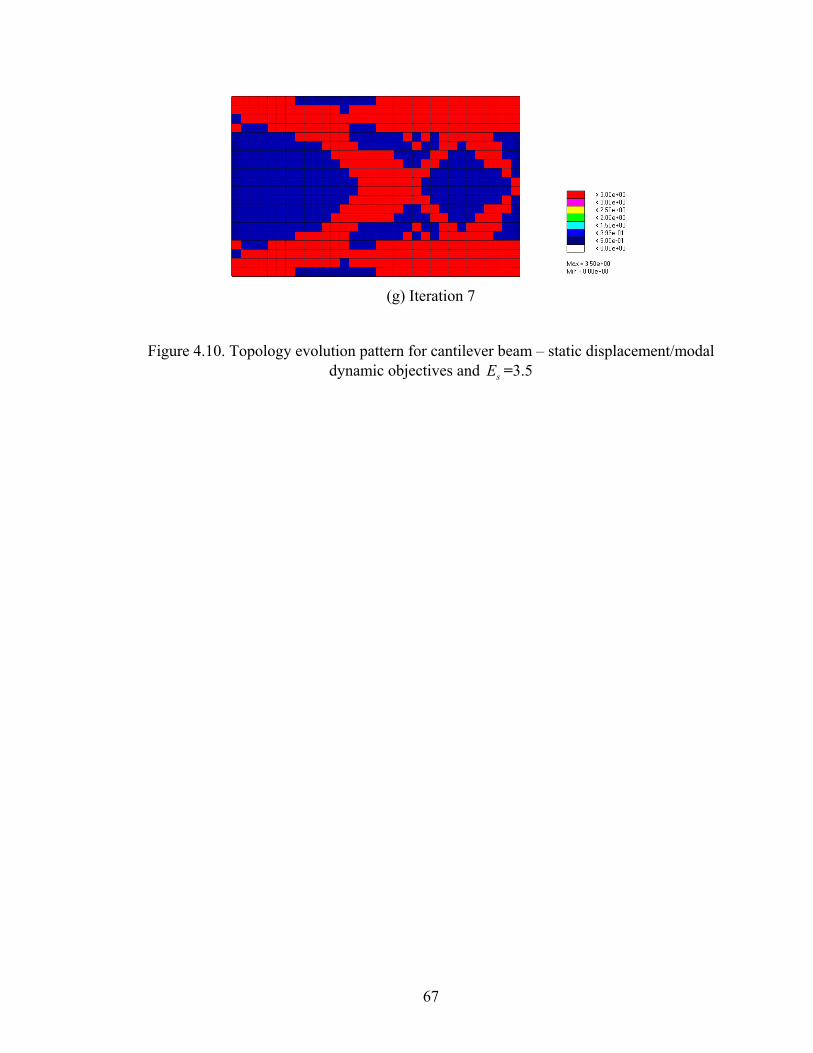
(g) Iteration 7
Figure 4.10. Topology evolution pattern for cantilever beam – static displacement/modal dynamic objectives and sE =3.5

68
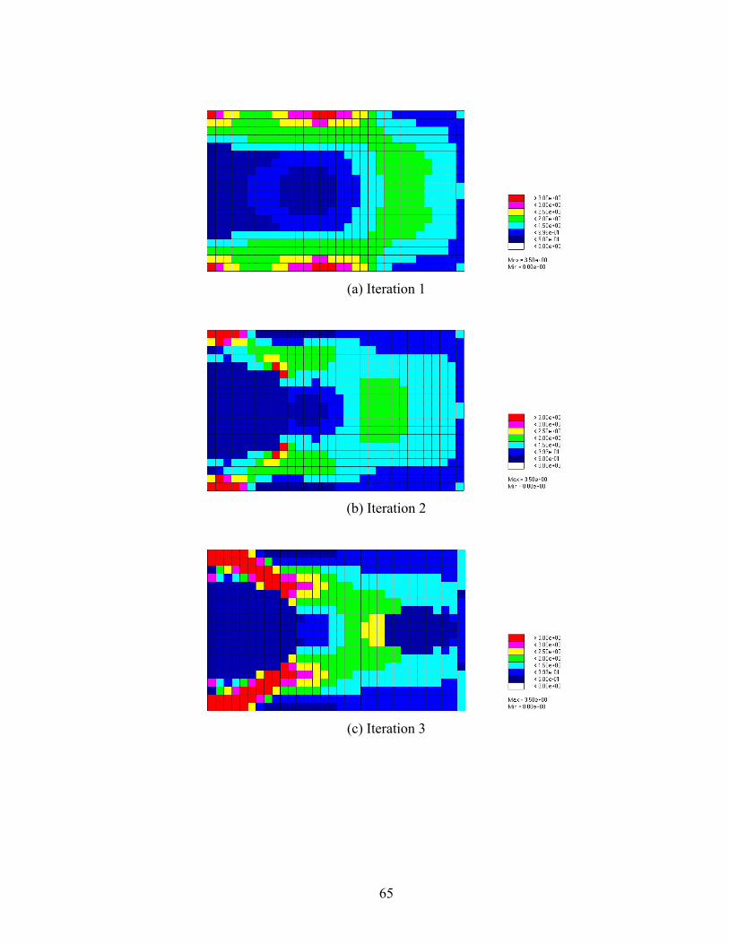
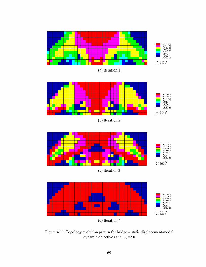
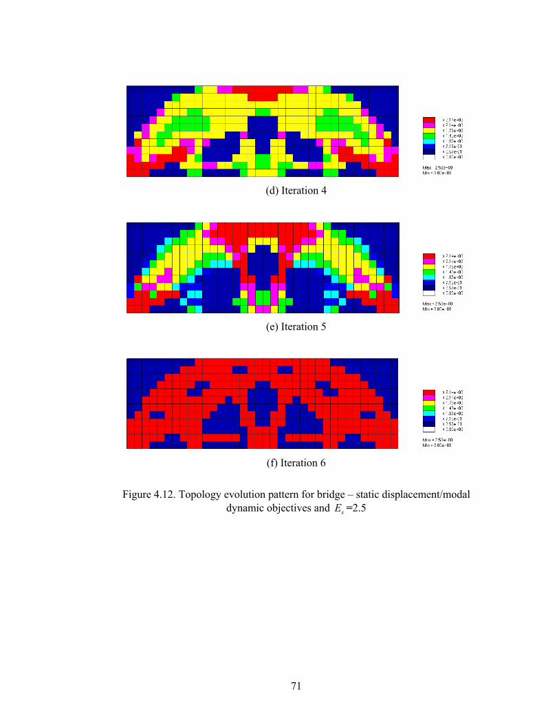
4.3.2. Bridge
For the bridge example, the evolved topology using target Young’s modulus 2.0
and 2.5 is shown in Figure 4.11 and Figure 4.12. For both cases, the results show similar
topology evolution patterns.
(a) The top part of the bridge and the end supports develop first, and then to the center of
the bridge. This occurs also in the static displacement example.
(b) The arch shape appears clearly from the early stage of evolutionary process and
remains to the end while detailed holes emerge in the later stage of the evolution process.
(c) For the stiffer material case, the holes become larger and larger as the iteration step
proceeds.
69
(a) Iteration 1
(b) Iteration 2
(c) Iteration 3
(d) Iteration 4
Figure 4.11. Topology evolution pattern for bridge – static displacement/modal
dynamic objectives and sE =2.0
70
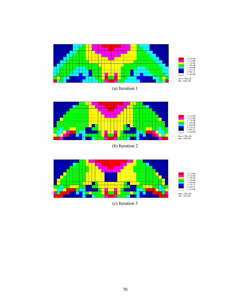
(a) Iteration 1
(b) Iteration 2
(c) Iteration 3
71
(d) Iteration 4
(e) Iteration 5
(f) Iteration 6
Figure 4.12. Topology evolution pattern for bridge – static displacement/modal
dynamic objectives and sE =2.5

72
CHAPTER V
CONCLUSIONS
In this dissertation, a topology evolution algorithm for Evolutionary Structural
Optimization (ESO) using LargE Admissible Perturbations (LEAP) was developed,
implemented and tested. In Section 5.1, the dissertation contributions are summarized. A
series of concluding remarks is given in Section 5.2. Finally, in Section 5.3, suggested
future research is recommended.
5.1. Dissertation Contributions
The main contributions of the present work can be summarized as follows:
(1) The ESO methodology as described in the literature cannot handle
multicriterion constraints efficiently. There was only a single attempt to solve
minimization of mean compliance (maximization of stiffness) and maximizing first
natural frequency simultaneously using Evolutionary Structural Optimization (ESO) with
the weighting method [14]. However, the results are limited to presenting different
topological structures by varying weighting criteria, not achieving a specific value of
performance constraints. The LargE Admissible Perturbation (LEAP) methodology
handles multiple performance constraints and therefore the ESO developed in this thesis
is not subject to the above limitation.
(2) Previous ESO methods use material density ρ set equal to 0 or 1 as design
variable. They cannot vary Young’s modulus and can only use initial Young’s modulus
of a fixed value. But ESO using LEAP methodology allows to change Young’s modulus

73
to achieve better structural performance with various Young’s modulus values while at
the same time eliminating mass as needed.
(3) Most methodologies for topology optimization in the literature require 40 to
100 numerical iterations. Current topology optimization methods using ESO still require
at least 60~70 iterations to converge [15], while ESO using the LEAP methodology only
takes 3 to 7 iterations to obtain converged results, thus, showing advanced computational
efficiency.
(4) Stabilized the optimization algorithm and improved computational efficiency
by developing the Cumulative Energy Elimination Rate (CEER) scheme. Compared to
the results of using fixed rate elimination method, less number of iterations is achieved
by developing the CEER scheme. If the fixed rate elimination scheme is applied,
convergence is not always guaranteed because there is a possibility that it might remove
some useful elements causing the structure to disappear in the later stage of the evolution
process.
(5) Most of the topology optimization methods in the literature impose volume
constraints while setting minimizing compliance as objective function. Since the
ESO/LEAP methodology does not have volume constraints, it was difficult to compare
the results of the current methodology to other topology optimization results. In this work,
numerical examples are used to show that the volume can be adjusted by controlling
performance constraint values. The results of ESO/LEAP methodology can be related to
results of other methods by changing the values of performance constraints.
(6) Similar topological results can be obtained with increased number of elements
in finite element analysis still achieving advanced computational efficiency. Benchmark
examples were tested to show that the result using higher resolution finite element mesh
exhibit very similar characteristics compared to coarse mesh examples still with few
iterations of finite element analysis required for convergence.

74
5.2. Concluding Remarks
An Evolutionary Structural Optimization algorithm using the Large Admissible
Perturbation method was developed. The cumulative energy elimination scheme was
proposed to remove the ineffective finite elements at each iteration. The advantages of
the current method can be summarized as: (1) ESO using the LEAP methodology
presented in this work can achieve an optimal topology that satisfies single/multiple
objectives with very few iterations and only two finite element analyses per iteration. It
only takes as few as 3 to 7 iterations to obtain converged results showing advanced
computational efficiency. (2) The ESO/LEAP methodology can handle multiple
performance design objectives such as static displacement and modal dynamic. Unlike
the other ESO/BESO methods reported in the literature, the current method can deal with
multiple objectives effectively since the LEAP methodology handles multiple
performance constraints. (3) ESO/LEAP can vary the target material stiffness, which
allows a designer to obtain various evolved structures satisfying multiple design
constraints. (4) Implementing the Cumulative Energy Elimination Rate (CEER) scheme
stabilized the optimization algorithm and improved computational efficiency. Compared
to the results of using fixed rate elimination method, smaller number of iterations is
achieved by developing the CEER scheme. (5) Showed that volume can be adjusted by
controlling performance constraints values in ESO/LEAP methodology. The results of
the current methodology can be related to other topology optimization results in the
literature which usually impose volume constraints. (6) Similar results are obtained with
increased number of mesh in finite element analysis still achieving advanced
computational efficiency.
Two benchmark applications, cantilever beam and bridge, are presented with
multiple numerical applications to show the effectiveness of the developed methodology.
The topological features of the results can be justified intuitively depending on the
performance objectives.
The ESO methodology as described in the literature cannot handle multicriterion
constraints efficiently. There has been only a single attempt to solve minimization of
75
mean compliance (maximization of stiffness) and maximizing first natural frequency
simultaneously using Evolutionary Structural Optimization (ESO) with the weighting and
global criterion method (Proos K.A., et al.[14]). However, the results are limited to
presenting different topological structures by varying weighting criteria, not achieving
specific values of performance constraints. The LargE Admissible Perturbation (LEAP)
methodology handles multiple performance constraints and therefore the ESO developed
in this work is not subject to the above limitation.
5.3. Suggested Future Work
The following future research is recommended:
(1) Improve ESO/LEAP methodology with Bi-directional Evolutionary Structural
Optimization. The present algorithm developed is based on only elimination of low
energy elements starting from a solid block structure. It cannot impose volume
constraints as target objectives like other ESO algorithms. By applying Bi-directional
Evolutionary Structural Optimization to the ESO/LEAP method, robustness can be
further enhanced.
(2) Extend the ESO/LEAP methodology with additional structural constraints. In
the present cases, the performance constraints applied were static displacement and
modal dynamic only. New and richer structural topologies can be created imposing other
constraints such as static stress and forced response amplitudes applied independently or
in combinations.
(3) Improve the nonlinear optimization process in order to deal with much larger
number of variables and constraints. The current FSQP (Feasible Sequential Quadratic
Programming) algorithm does not provide sufficient options to adjust the optimization
process in case of failure to search for converging solutions.

76
APPENDIX A
General Perturbation Equation for Static Deflection with Static Mode Compensation
The following derivation is based on the work of Bernitsas and Suryatama [25].
(a) Static Mode Compensation
Assuming that { } { }f f′ = which implies that f does not depend on allowed
geometric changes ( eα ’s), the static equilibrium equation of the unknown State S2 can be
written as
[ ]{ } { }k u f′ ′ = , (A.1)
Define { }Q′ as transformed displacement vector, then the predicted static
deflection { }u′ can be approximated by including the static deflection mode of the
baseline structure { }u .
{ } { } [ ]{ }u u Q′ ′ ′= + Φ , (A.2)
where [ ]′Φ is the matrix of the mode shape vectors of the unknown State S2 which are
1 2[ ] [{ } ,{ } , ,{ } ]rnφ φ φ′ ′ ′ ′Φ = .

77
Substituting (A.2) into (A.1) gives
[ ]{ } [ ][ ][ ] { }k u k Q f′ ′ ′ ′+ Φ = (A.3)
Premultiply (A.3) by [ ]T′Φ yields
[ ] [ ]{ } [ ] [ ][ ]{ } [ ] { }T T Tk u k Q f′ ′ ′ ′ ′ ′ ′Φ + Φ Φ = Φ (A.4)
Since the generalized stiffness matrix is defined as
[ ] [ ] [ ][ ]TK k′ ′ ′ ′= Φ Φ , (A.5)
And equation (A.4) can be written as
[ ]{ } [ ] { } [ ] [ ]{ }T TK Q f k u′ ′ ′ ′ ′= Φ − Φ (A.6)
Using equation (2.19), equation (A.6) can be rewritten as
[ ]{ } [ ] [ ]{ }TK Q k u′ ′ ′= − Φ ∆ (A.7)
Premultiplying each side by 1[ ]K −′ which is equal to [1/ ]K ′ , gives the following equation
for the transformed displacement vector { }Q′ ,
{ } [1/ ][ ] [ ]{ }TQ K k u′ ′ ′= − Φ ∆ (A.8)
Substituting equation (A.8) into (A.2) yields the predicted static deflection in a form that
includes no matrix inversion
{ } { } [ ][1/ ][ ] [ ]{ }Tu u K k u′ ′ ′ ′= − Φ Φ ∆ (A.9)
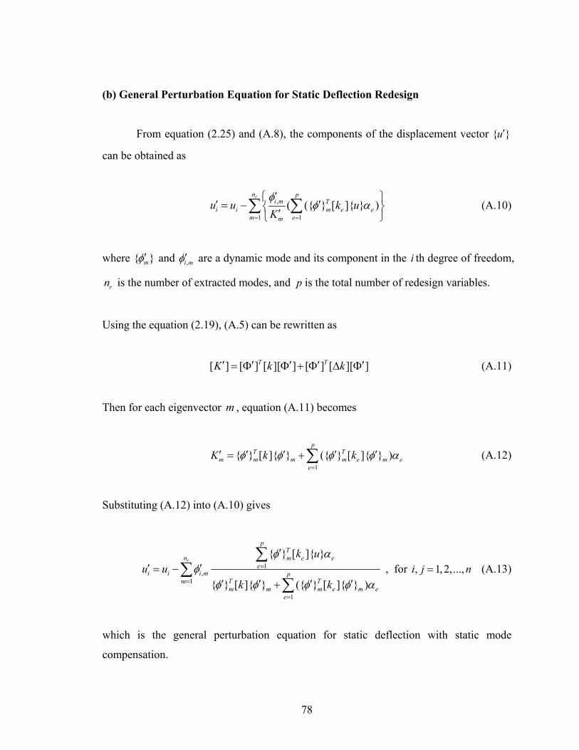
78
(b) General Perturbation Equation for Static Deflection Redesign
From equation (2.25) and (A.8), the components of the displacement vector { }u′
can be obtained as
,
1 1( ({ } [ ]{ } )
rn pi m T
i i m e em em
u u k uKφ
φ α= =
′⎧ ⎫′ ′= − ⎨ ⎬′⎩ ⎭
∑ ∑ (A.10)
where { }mφ′ and ,i mφ′ are a dynamic mode and its component in the i th degree of freedom,
rn is the number of extracted modes, and p is the total number of redesign variables.
Using the equation (2.19), (A.5) can be rewritten as
[ ] [ ] [ ][ ] [ ] [ ][ ]T TK k k′ ′ ′ ′ ′= Φ Φ + Φ ∆ Φ (A.11)
Then for each eigenvector m , equation (A.11) becomes
1
{ } [ ]{ } ({ } [ ]{ } )p
T Tm m m m e m e
e
K k kφ φ φ φ α=
′ ′ ′ ′ ′= +∑ (A.12)
Substituting (A.12) into (A.10) gives
1,
1
1
{ } [ ]{ }
{ } [ ]{ } ({ } [ ]{ } )
r
pT
n m e ee
i i i m pT Tmm m m e m e
e
k uu u
k k
φ αφ
φ φ φ φ α
=
=
=
′′ ′= −
′ ′ ′ ′+
∑∑
∑ , for , 1, 2,...,i j n= (A.13)
which is the general perturbation equation for static deflection with static mode
compensation.
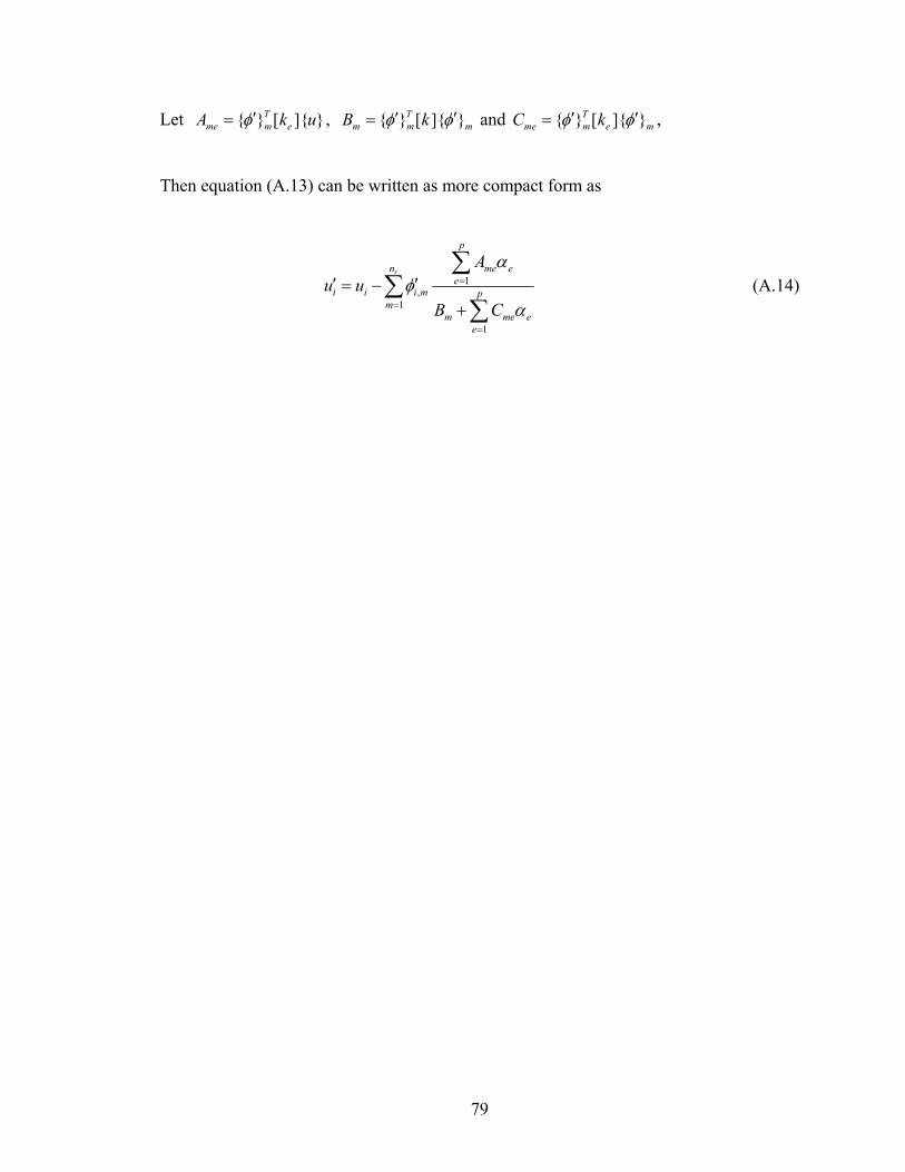
79
Let { } [ ]{ }Tme m eA k uφ′= , { } [ ]{ }T
m m mB kφ φ′ ′= and { } [ ]{ }Tme m e mC kφ φ′ ′= ,
Then equation (A.13) can be written as more compact form as
1,
1
1
r
p
n me ee
i i i m pm
m me ee
Au u
B C
αφ
α
=
=
=
′ ′= −+
∑∑
∑ (A.14)

80
APPENDIX B
General Perturbation Equation for Modal Dynamics
Define generalized mass matrix of the objective structure as
[ ] [ ] [ ][ ]TM m′ ′ ′ ′= Φ Φ (B.1)
where [ ]′Φ is the matrix of the mode shape vectors of the unknown State S2.
Also define the structural perturbations for eigenvalues as
2 2 2[ ] [ ] [ ]ω ω ω′ = + ∆ (B.2)
Premultiplying [ ]T′Φ to equation (2.18) gives the modal equation for the unknown State
S2.
2[ ] [ ][ ]K M ω′ ′ ′= (B.3)
Substituting the equations (2.19)-(2.21), (B.2) and (2.25)-(2.26) which are the linear
relationships of eα between stiffness and mass matrix into (B.3), we get
2 2
1({ } [ ]{ } { } [ ]{ } ) { } [ ]{ } { } [ ]{ }
pT T T T Tj e i i j e i e i j i j e i
ek m m kφ φ ω φ φ α ω φ φ φ φ
=
′ ′ ′ ′ ′ ′ ′ ′ ′ ′− = −∑ ,
for , 1, 2,...,i j n= (B.4)
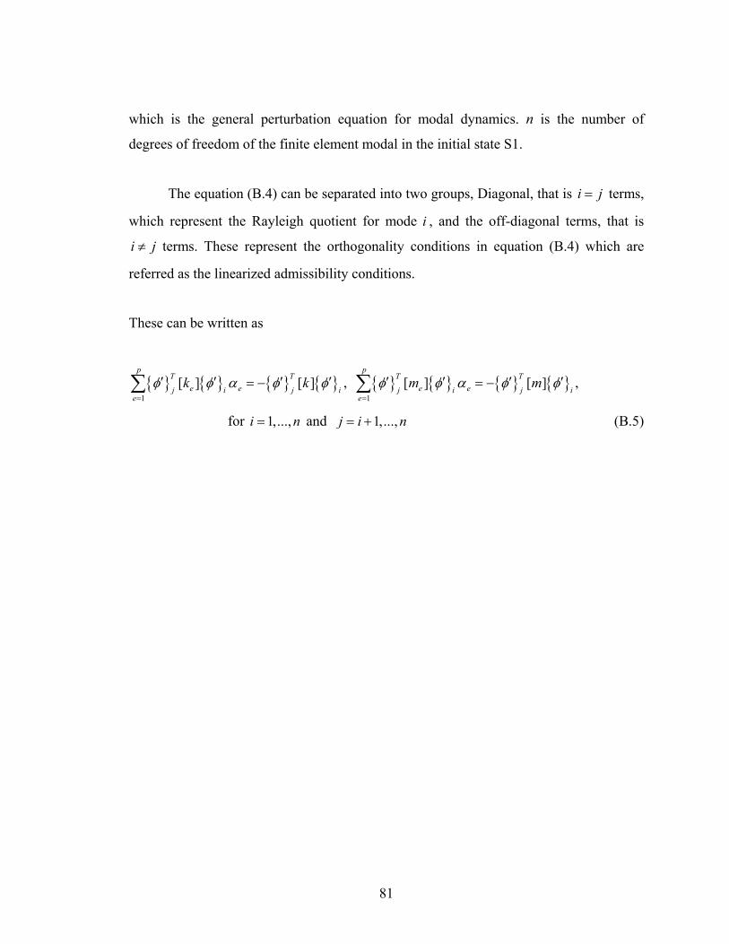
81
which is the general perturbation equation for modal dynamics. n is the number of
degrees of freedom of the finite element modal in the initial state S1.
The equation (B.4) can be separated into two groups, Diagonal, that is i j= terms,
which represent the Rayleigh quotient for mode i , and the off-diagonal terms, that is
i j≠ terms. These represent the orthogonality conditions in equation (B.4) which are
referred as the linearized admissibility conditions.
These can be written as
{ } { } { } { }1
[ ] [ ]p
T Te ej i j i
e
k kφ φ α φ φ=
′ ′ ′ ′= −∑ , { } { } { } { }1
[ ] [ ]p
T Te ej i j i
e
m mφ φ α φ φ=
′ ′ ′ ′= −∑ ,
for 1,...,i n= and 1,...,j i n= + (B.5)

82
APPENDIX C
Linear Prediction for Eigenvectors
In matrix form, the i th mode free vibration equation for the initial and objective
structures can be written as
2[ ]{ } [ ]{ }i i ik mφ φ ω= (C.1)
2[ ]{ } [ ]{ }i i ik mφ φ ω′ ′ ′ ′ ′= (C.2)
where 2iω is the i th eigenvalue corresponding to the i th eigenvector { }iφ .
Premultiplying equation (C.2) by { }Tiφ′ and using the perturbation relations
(2.19)-(2.21) and (B.2), we derive an equation that can be developed into 24 terms among
which 15 are nonlinear terms in 2[ ( )]∆… and 3[ ( )]∆… .
From this point, we assume small perturbations in order to linearize this equation
by keeping the nine linear terms as follows
{ } [ ]{ } { } [ ]{ } { } [ ]{ } { } [ ]{ }T T T Tj i j i j i j ik k k kφ φ φ φ φ φ φ φ+ ∆ + ∆ + ∆
2 2 2{ } [ ]{ } { } [ ]{ } { } [ ]{ }T T Tj i i j i i j i im m mφ φ ω φ φ ω φ φ ω= + ∆ + ∆
2 2{ } [ ]{ } { } [ ]{ }T Tj i i j i im mφ φ ω φ φ ω+ ∆ + ∆ (C.3)
For i j= , using equation (C.1) and its transpose, we get

83
2 2{ } [ ]{ } { } [ ]{ }T T
i i i i i i ik m Mφ φ φ φ ω ω∆ − ∆ = ∆ (C.4)
where iM is the i th diagonal term of the generalized mass matrix defined in (B.1). For
i j≠ , { } [ ]{ } 0Tj imφ φ = and using the transpose of (C.1) for j th mode, equation (C.3)
becomes
2 2 2{ } [ ]{ } { } [ ]{ } { } [ ]{ } ( )T T T
j i j i i j i i jk m mφ φ φ φ ω φ φ ω ω∆ − ∆ = ∆ − (C.5)
Assuming that the changes in eigenvectors can be written as
[ ] [ ][ ]TG∆Φ = Φ (C.6)
where [G] is the matrix of admixture coefficients with 0iiG = and ijG small for i j≠ .
The matrix calculation in (C.6) can be written as
, ,1
rn
i m i k mkk
Gφ φ=
∆ =∑ (C.7)
where i corresponds to the degree of freedom and m to the mode vector, can be referred
as a reduced basis method. mkG corresponds to the contribution factor of mode k to a
change in mode m . Physical meaning of equation (C.7) can be described as follows. For
a three dimensional structure, three major mode shapes exists such as stretching, bending
and torsional modes. However, one type of mode has little effect on the other modes,
which leads to small values of admixture coefficient, ijG .
Substituting equation (C.6) into (C.5), gives
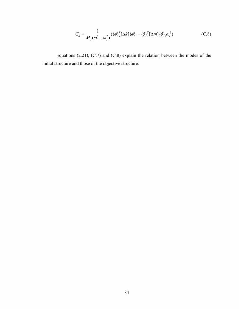
84
22 2
1 ({ } [ ]{ } { } [ ]{ } )( )
T Tij j i j i i
j i j
G k mM
φ φ φ φ ωω ω
= ∆ − ∆−
(C.8)
Equations (2.21), (C.7) and (C.8) explain the relation between the modes of the
initial structure and those of the objective structure.

85
APPENDIX D
Feasible Sequential Quadratic Programming (FSQP)
This appendix is from the FSQP reference manual [32] by Institute for System
Research (ISR), University of Maryland. FSQP is an open source code for minimization
of the maximum of a set of smooth objective functions subject to general smooth
constraints.
The FSQP algorithm is a superlinearly convergent algorithm for directly tackling
optimization problems with multiple linear/nonlinear objective functions (minimax),
linear/nonlinear inequality constraints, linear/nonlinear equality constraints.
The general optimization problem can be formulated as follows:
min max{ ( )}f ix X i I
f x∈ ∈
(D.1)
where {1, , }ffI n= … and X is the set of points nx R∈ satisfying
bl x bu≤ ≤ (boundary constraints) (D.2)
( ) 0, 1,j iG x j N≤ = … (nonlinear inequality constraints) (D.3)
( ) 0, 1, ,j ig x j n≤ = … (linear inequality constraints) (D.4)
( ) 0, 1, ,j eH x j N= = … (nonlinear equality constraints) (D.5)
( ) 0, 1, ,j eh x j n= = … (linear equality constraints) (D.6)
86
with ; ; : , 1, ,n n ni fbl R bu R f R R i n∈ ∈ → = … smooth; : , 1, ,n
i iG R R j N→ = … nonlinear
and smooth; : , 1, ,ni ig R R j n→ = … linear; : , 1, ,n
i eH R R j N→ = … nonlinear and
smooth; : , 1, ,ni eh R R j n→ = … linear. It is allowed to have 0fn = , in which case
problem (D.1) is one of finding a point that satisfies a given set of constraints.
Key features related to the present research are as follows:
(1) All nonlinear equality constraints are turned into inequality constraints. Nonlinear
equality constraints are changed to inequality constraints and the maximum of the
objective function is replaced by an exact penalty function that penalizes nonlinear
equality constraint violations only.
(2) Ability to search for an initial feasible point satisfying all linear constraints and
nonlinear inequality constraints. That is, it is capable of generating iterations satisfying
all linear constraints and nonlinear inequality constraints (mandatory for many
applications) starting from a feasible point. If the initial guess provided by the user is
infeasible for some inequality constraint or some linear equality constraint, FSQP first
generates a feasible point for these constraints; subsequently the successive iterates
generated by FSQP all satisfy these constraints.
(3) Ability to improve objective function after each iteration or after at most four
iterations (user’s option) if there is no nonlinear equality constraints. The user has the
option of either requiring that the objective function (penalty function if nonlinear
equality constraints are present) decrease at each iteration after feasibility for nonlinear
inequality and linear constraints has been reached (monotone line search), or requiring a
decrease within at most four iterations (non-monotone line search). The user must
provide functions that define the objective functions and constraint functions and may
either provide functions to compute the respective gradients or require that FSQP
estimate them by forward finite differences.

87
FSQP is an implementation of two algorithms based on Sequential Quadratic
Programming (SQP), modified so as to generate feasible iterates. In the first one
(monotone line search), a certain Armijo type arc search is used with property that the
step of one is eventually accepted, a requirement for superlinear convergence. In the
second one, the same effect is achieved by means of a non-monotone search along a
straight line. The merit function used in both searches is the maximum of the objective
functions if there is no nonlinear equality constraint, or an exact penalty function if
nonlinear equality constraints are present.
88
BIBLOGRAPHY
1. Cheng G.D., Olhoff N., “An investigation concerning optimal design of solid elastic plates”, International Journal of Solids and Structures, 1981, 17:305-323. 2. Bendsøe M.P., Kikuchi N., “Generating Optimal Topology in Structural Design Using a Homogenization Method”, Computer Methods in Applied Mechanics and Engineering, 1988, 71:197-224.
3. Bendsøe M.P., “Optimal Shape Design as a Material Distribution Problem”, Structural and Multidisciplinary Optimization, 1989, 1: 193-202.
4. Suzuki K., Kikuchi N., “A homogenization method for shape and topology optimization”, Computer Methods in Applied Mechanics and Engineering, 1991, 93:291-318.
5. Ma Z.D., Kikuchi N., Cheng H.C., “Topological Design for Vibrating Structures”, Computer Methods in Applied Mechanics and Engineering, 1995, 121:259-280.
6. Pederson N.L., “Maximization of Eigenvalues”, Structural and Multidisciplinary Optimization, 2000, 20: 2-11.
7. Yang R.J., Chuang C.H., “Optimal Topology Design Using Linear Programming”, Computers and Structures, 1994, 52-2:265-275.
8. Xie Y.M., Steven G.P., “A Simple Evolutionary Procedure for Structural Optimization”, Computers and Structures, 1993, 49:885-896.
9. Chu D.N., Xie Y.M., Hira A., and Steven G.P., “Evolutionary Structural Optimization for Problems with Stiffness Constraints”, Finite Elements in Analysis and Design, 1996, 21(3):239-251.

89
10. Zhao C., Steven G.P. and Xie Y.M., “Evolutionary Natural Frequency Optimization of Thin Plate Bending Vibration Problems”,Structural Optimization,1996, 11:244-251.
11. Manickarajah D.,Xie Y.M. and Steven G.P., “An Evolutionary Method for Optimization of Plate Buckling Resistance”, Finite Elements in Analysis and Design, 1998, 29(3):205-230.
12. Li Q., Steven G.P. and Xie Y.M., “Optimal Shape Design for Steady Heat Conduction by the Evolutionary Procedure”, Inverse Problems in Heat Transfer and Fluid Flow, 1997, Heat Transfer Div. American Society of Mechanical Engineers, New York, 340:159-164.
13. Querin O.M., Young V., Xie Y.M., Steven GP, “Computational Efficiency and Validation of Bi-directional Evolutionary Structural Optimization”, Computer Methods in Applied Mechanics and Engineering, 2000, 189:559-573.
14. Proos K.A., Steven G.P., O.M. Querin and Xie Y.M., “Multicriterion Evolutionary Structural Optimization Using the Weighting and the Global Criterion Methods”,AIAA Journal, 2001, 39(10):2006-2012.
15. Huang X., Xie Y.M., “Convergent and Mesh-independent Solutions for the Bi-directional Evolutionary Structural Optimization Method”, Finite Elements in Analysis and Design, 2007, 43:1039-1049.
16. Huang X., Xie Y.M., “Bi-directional evolutionary topology optimization of continuum structures with one or multiple materials”, Comput. Mech., 2009, 43:393-401.
17. Huang X., Xie Y.M., “Optimal design of periodic structures using evolutionary topology optimization”, Structural and Multidisciplinary Optimization, 2007, 36(6): 597-606.
18. Stetson K.A., Palma, G.E., “Inversion of First-Order Perturbation Theory and Its Application to Structural Design”, AIAA Journal, 1976, 14(4):454-460.
19. Sandström R.E., Anderson W.J., “Modal Perturbation Methods for Marine Structures”, SNAME Transactions, 1982, 90:41-54.
20. Stetson K.A., Harrison I.R., “Redesign of Structural Vibration Modes by Finite Element Inverse Perturbation”, Journal of Engineering for Power, ASME Transactions, 1981, 103(2): 319-325.

90
21. Hoff J., Bernitsas M.M., “Dynamic Redesign of Marine Structures”, Journal of Ship Research, 1985, 29: 285–295.
22. Kim J.H., Bernitsas M.M., “Redesign of Marine Structures”, Marine Structures, 1990, 1(2):139-183.
23. Bernitsas M.M., Tawekal R.L., “Structural Model Correlation using Large Admissible Perturbation in Cognate Space”, AIAA Journal, 1991, 29(12):2222-2232.
24. Bernitsas M.M., Rim W., “Redesign of Plates by Large Admissible Perturbations”, AIAA Journal, 1994, 32: 1021–1028.
25. Bernitsas M.M., Suryatama D., “Structural Redesign by Large Admissible Perturbations with Static Mode Compensation”, Journal of Offshore Mechanics and Arctic Engineering, 1999, 121(1):39-46.
26. Bernitsas M.M., Blouin V.Y., “Structural Redesign for Forced Response Amplitude with Proportional Damping by Large Admissible Perturbations”, AIAA Journal, 1999, 37(11):1506-1513.
27. Bernitsas M.M., Kristanto B.K., “Static Stress Redesign of Structures by Large Admissible Perturbations”, Journal of Offshore Mechanics and Arctic Engineering, 2003, 127:122-129.
28. Blouin V.Y., Bernitsas M.M., “Cognate Space Identification for Forced Response Structural Redesign”, Journal of Offshore Mechanics and Arctic Engineering, 2005, 127(3):227-233.
29. Suryatama D., Bernitsas M.M., “Topology and Performance Redesign of Complex Structures by Large Admissible Perturbations”, Structural and Multidisciplinary Optimization, 2000, 20:138-153.
30. Miao L., Bernitsas M.M., “Topology Redesign for Performance by Large Admissible Perturbations”, Structural and Multidisciplinary Optimization, 2006, 31:117-133. 31. Earmme T., Bernitsas M.M., “Parametric Evolution of Structural Topology by Large Admissible Perturbations”, 7th World Congress of Structural and Multidisciplinary Optimization, 2007, Seoul Korea.
91
32. Zhou, J.L.,Tits, A.L. and Lawrence, C.T., User’s Guide for FFSQP Version 3.7:A FORTRAN Code for Solving Constrained Nonlinear (Minimax) Optimization Problems, Generating Iterates Satisfying All Inequality and Linear Constraints, Electrical Engineering Department and Institute of Systems Research, University of Maryland, College Park. MD 20742, 1997.
33. MSC/NASTRAN Version 70.0 Advanced Dynamics User’s Guide, MacNeal-Schwandler Corporation, Los Angeles, CA., November 1989.
Related Documents