Evolution of Coordination and Communication in Groups of Embodied Agents ( ) by Olaf Khang Witkowski A Doctoral Thesis Submitted to the Graduate School of the University of Tokyo on December 12, 2014 in Partial Fulfillment of the Requirements for the Degree of Doctor of Information Science and Technology in Computer Science Thesis Supervisor: Takashi Ikegami Official Supervisor: Reiji Suda Professors of Computer Science

Welcome message from author
This document is posted to help you gain knowledge. Please leave a comment to let me know what you think about it! Share it to your friends and learn new things together.
Transcript
Evolution of Coordination andCommunication in Groups of Embodied Agents(��������������������
����������������)
by
Olaf Khang Witkowski
��� ���� �������
A Doctoral Thesis
����
Submitted to
the Graduate School of the University of Tokyo
on December 12, 2014
in Partial Fulfillment of the Requirements
for the Degree of Doctor of Information Science and Technology
in Computer Science
Thesis Supervisor: Takashi Ikegami �� ��
O�cial Supervisor: Reiji Suda �� ��
Professors of Computer Science
ABSTRACT
From biological cells to bee swarms and bird flocks, nature shows countless examples of
self-organized groups displaying a collective mind. In such species, individuals interacting
together end up producing an emergent behavior that increases their chances of survival
and reproduction.
This thesis shows an exploration of the evolution of communication through coordinated
behaviors in populations of embodied agents. The goal is to reach a better understanding
of nature’s conditions for the evolution and strategies for the maintenance of collective
behaviors.
For that purpose, we present a framework making use of agent-based modeling to
study the parallel evolution of coordination, cooperation and communication, for di↵erent
types of interactions and levels of complexity. Through computer simulations, we test
hypotheses on the conditions leading to synergistic behaviors and the evolution of honest
communication.
We first show signal-based swarming, in a population where the information exchanged
between agents via signaling is able to form temporary leader-follower relationships, allow-
ing them to flock together. Next, the emergence of static clusters of agents is investigated
in the case of a dynamic variant of the spatial prisoner’s dilemma, in which multistable
strategies exhibit formation and destruction of cooperative nuclei. After that, we study
the adaptation of social coordination in dynamic environments. By the use of agent-based
models, we show the evolutionary stability of cooperation, expressed as behaviors ranging
from migration to specific resource-saving strategies. Finally, we develop a model of genetic
and cultural evolution, implementing the niche-construction of language, where the bio-
logical selection on the genes is repeatedly masked, then unmasked by cultural evolution.
These results show how simple agents can reach higher-order computational capabilities
through the evolution of collective behavior. By self-organizing in collaborative groups,
individuals are able to overcome local errors and fluctuations in the environment, allowing
them to exploit more e�ciently the information present in the environment to reach higher
performance and thus fitness.
This study is significant for both scientific and technological reasons. Indeed, on the one
hand, it contributes to shed light on the evolution of coordination and communication. On
the other hand, a better understanding of the fundamental principles of collective behavior
may also lead to innovative methods in multi-agents systems, ubiquitous computing devices
and swarm computation.

����
���������������������������������������
��������������������������������������
���������������������������������������
���������������������������������������
���������������������������������������
���������������������������������������
��������������������������������������
���������������������������������������
���������������������������������������
����������
������������������������������������
���������������������������������������
���������������������������������������
���������������������������������������
��������������������������������������
���������������������������������������
���������������������������������������
���������������������������������������
���������������������������������������
���������������������������������������
���������������������������������������
��������������
�������������������������������������
���������������������������������������
���������������������������������������
��������������������
Contents
1 Introduction 1
1.1 Thesis overview . . . . . . . . . . . . . . . . . . . . . . . . . . . . . . . . . . . 4
1.2 Summary of contributions . . . . . . . . . . . . . . . . . . . . . . . . . . . . . 6
2 Background review 8
2.1 The process of evolution . . . . . . . . . . . . . . . . . . . . . . . . . . . . . . 8
2.2 Emergence of coordination . . . . . . . . . . . . . . . . . . . . . . . . . . . . . 13
2.3 Evolution of cooperation . . . . . . . . . . . . . . . . . . . . . . . . . . . . . . 15
2.4 Evolution of communication . . . . . . . . . . . . . . . . . . . . . . . . . . . . 20
2.5 Intricacies of human language . . . . . . . . . . . . . . . . . . . . . . . . . . . 22
3 Methods 25
3.1 Agent-based modeling as a tool . . . . . . . . . . . . . . . . . . . . . . . . . . 25
3.2 Recent model-based approaches . . . . . . . . . . . . . . . . . . . . . . . . . . 29
3.3 Artificial neural networks . . . . . . . . . . . . . . . . . . . . . . . . . . . . . 29
3.4 Neuroevolution . . . . . . . . . . . . . . . . . . . . . . . . . . . . . . . . . . . 35
4 Signal-based coordination and neutral selection 39
4.1 Swarming behavior . . . . . . . . . . . . . . . . . . . . . . . . . . . . . . . . . 39
4.2 Asynchronous agent-based simulation . . . . . . . . . . . . . . . . . . . . . . 43
4.3 Results . . . . . . . . . . . . . . . . . . . . . . . . . . . . . . . . . . . . . . . . 46
4.4 Discussion . . . . . . . . . . . . . . . . . . . . . . . . . . . . . . . . . . . . . . 59
5 Cooperative coordination in a dynamic spatial Prisoner’s Dilemma 63
5.1 Spatial Prisoner’s Dilemma . . . . . . . . . . . . . . . . . . . . . . . . . . . . 64
5.2 Model . . . . . . . . . . . . . . . . . . . . . . . . . . . . . . . . . . . . . . . . 65
5.3 Results . . . . . . . . . . . . . . . . . . . . . . . . . . . . . . . . . . . . . . . . 69
i
5.4 Analysis of cooperation and clustering . . . . . . . . . . . . . . . . . . . . . . 72
5.5 Discussion . . . . . . . . . . . . . . . . . . . . . . . . . . . . . . . . . . . . . . 75
6 Synchronization in variable resource environments 77
6.1 Signaling in dynamic environments . . . . . . . . . . . . . . . . . . . . . . . . 78
6.2 Signal-based synchronization to environment variability . . . . . . . . . . . . 79
6.3 Mimicry and seasonal migratory synchronization . . . . . . . . . . . . . . . . 85
6.4 Periodic resource scarcity leads to size-dependent saving strategies . . . . . 91
7 Neutral selection in gene-culture coevolution 99
7.1 The Baldwin e↵ect . . . . . . . . . . . . . . . . . . . . . . . . . . . . . . . . . 100
7.2 A model of gene-culture coevolution . . . . . . . . . . . . . . . . . . . . . . . 101
7.3 Remarkable features of the model . . . . . . . . . . . . . . . . . . . . . . . . . 103
7.4 Discussion . . . . . . . . . . . . . . . . . . . . . . . . . . . . . . . . . . . . . . 111
8 Conclusion 114
8.1 Recapitulation and contributions . . . . . . . . . . . . . . . . . . . . . . . . . 115
8.2 Limitations . . . . . . . . . . . . . . . . . . . . . . . . . . . . . . . . . . . . . 117
8.3 Future directions . . . . . . . . . . . . . . . . . . . . . . . . . . . . . . . . . . 120
References 126
ii
List of Figures
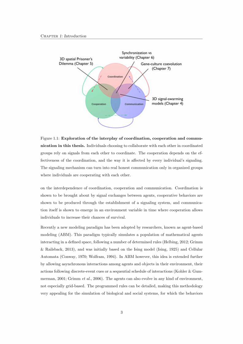
1.1 Exploration of the interplay of coordination, cooperation and com-
munication in this thesis. Individuals choosing to collaborate with each
other in coordinated groups rely on signals from each other to coordinate. The
cooperation depends on the e↵ectiveness of the coordination, and the way it
is a↵ected by every individual’s signaling. The signaling mechanism can turn
into real honest communication only in organized groups where individuals
are cooperating with each other. . . . . . . . . . . . . . . . . . . . . . . . . . 3
3.1 An example of artificial neural network. Each circular node represents
an artificial neuron and each arrow represents a connection from the output of
one neuron to the input of another. Image credit: Glosser.ca on Wikimedia,
licensed under Creative Commons. . . . . . . . . . . . . . . . . . . . . . . . . 31
3.2 An example of Elman simple recurrent neural network. The context
layer (u1
to ul) provides a limited memory e↵ect to the network, allowing for
pattern sequence prediction. Image credit: yedernoggersnodden on Wikime-
dia, licensed under Creative Commons. . . . . . . . . . . . . . . . . . . . . . 34
4.1 A murmuration of starlings in Gretna (Scotland). Image credit:
Flickr user ad551, licensed under Creative Commons. . . . . . . . . 40
iii
4.2 Visualization of the three successive phases in the training proce-
dure (from left to right: t = 0, t = 2 · 105, t = 2 · 107) in a typical
run. The simulation is with 200 initial agents and a single resource spot.
At the start of the simulation the agents have a random motion (a), then
progressively come to coordinate in a dynamic flock (b), and eventually clus-
ter more and more closely to the goal towards the end of the simulation (c).
The agents’ colors represent the signal they are producing, ranging from 0
(blue) to 1 (red). The goal location is represented as a green sphere on the
visualization. . . . . . . . . . . . . . . . . . . . . . . . . . . . . . . . . . . . . 47
4.3 Visualization of the swarming behavior occurring in the second
phase of the simulation. The figure represents consecutive shots each
10 iterations apart in the simulation. The observed behavior shows agents
flocking in dynamic clusters, rapidly changing shape. . . . . . . . . . . . . . 48
4.4 Comparison of the average number of neighbors (average over 10
runs, with 106 iterations) in the case signaling is turned on versus
o↵. . . . . . . . . . . . . . . . . . . . . . . . . . . . . . . . . . . . . . . . . 49
4.5 Plot of the average inward neighborhood transfer entropy for sig-
naling switched on (red curve) and o↵ (blue curve). The inward
neighborhood transfer entropy captures how much agents are “following” in-
dividuals located in their neighborhood at a given time step. The values
rapidly take o↵ on the regular simulation (with signaling switched on, see red
curve), whereas they remain low for the silent control (with signaling o↵, see
blue curve). . . . . . . . . . . . . . . . . . . . . . . . . . . . . . . . . . . . . 50
4.6 Plot of the individual outward neighborhood transfer entropy
(NTE), aiming to capture the change in leadership. The plot repre-
sents the average transfer entropy from an agent to its neighbors, capturing
the presence of local leaders in the swarming clusters. Each color corresponds
to a distinct agent. A succession of bursts is observed, each corresponding to
a di↵erent agent, indicating a continual change of leadership in the swarm. . 51
iv
4.7 Average distance of agents to the goal with signaling (top) and
a control run with signaling switched o↵ (bottom). The average
distance to the goal decreases between time step 105 and time step 2 ⇥ 105,
the agents eventually getting as close as 50 units away from the goal on
average. In the same conditions, the silenced control experiment results in
agents constantly remaining around 400 units away from the goal in average. 52
4.8 Plots of evolved agents’ motor responses to a range of value in input
and context neurons. The three axes represent signal input average values
(right horizontal axis), context unit average level (left horizontal axis), and
average motor responses (vertical axis). The top two graphs correspond to
the neural controllers of swarming agents, and the bottom ones correspond to
non-swarming ones’. . . . . . . . . . . . . . . . . . . . . . . . . . . . . . . . . 53
4.9 Architecture of the agent’s controller, a recursive neural network
composed of 6 input neurons (I1
to I6
) , 10 hidden neurons (H1
to
H10
) , 10 context neurons (C1
to C1
0) and 3 output neurons (O1
to
O3
). The input neurons receive signal values from neighboring agents, with
each neuron corresponding to signals received from one of the 6 sectors in
space. The output neurons O1
and O2
control the agent’s motion, and O3
controls the signal it emits. . . . . . . . . . . . . . . . . . . . . . . . . . . . . 54
4.10 Invasion of freeriders resulting from the introduction of 5 silent
individuals in the population. About 200k iterations after their intro-
duction, the 5 freeriders have replicated and taken over the whole population.
. . . . . . . . . . . . . . . . . . . . . . . . . . . . . . . . . . . . . . . . . . . . 55
4.11 Average signal intensity over the population versus evolutionary
time (5 runs). . . . . . . . . . . . . . . . . . . . . . . . . . . . . . . . . . . 55
4.12 Genotypic diversity measured by Shannon’s information entropy.
The information entropy measures the variety in the measure progressively
decreases during the simulation, until it reaches a minimal value of 50 hartleys
(information unit corresponding to a base 10 logarithm) around the millionth
iteration, then restarts to increase slowly. . . . . . . . . . . . . . . . . . . . . 56
4.13 Phylogenetic tree of agents created during a run. The center corre-
sponds to the start of the simulation. Each branch represents an agent, and
every fork corresponds to a reproduction process. . . . . . . . . . . . . . . . 57
v
4.14 Top plot: average number of neighbors during a single run. Bot-
tom plot: agents phylogeny for the same run. The roots are on
the left, and each bifurcation represents a newborn agent. The two
plots show the progression of the average swarming in the population, indi-
cated by the average number of neighbors through the simulation, compared
with a horizontal representation of the phylogenetic tree. Around iteration
400k, when the neighborhood becomes denser, the selection on agents’ ability
to swarm together is apparently relaxed due to the signaling pattern being
largely spread. This leads to higher heterogeneity, as can be seen on the
upper plot, with numerous genetic branches forming towards the end of the
simulation. . . . . . . . . . . . . . . . . . . . . . . . . . . . . . . . . . . . . . 58
4.15 Biplot of a PCA on the genotypes of all agents of the simulation.
Each circle represents one agent’s genotype, the diameter representing the
average number of neighbors over the lifetime of the agent, and the color
showing its time of death ranging from bright green (at time step 0, early in
the simulation) to red (at time step 106, towards the end of the simulation). 59
5.1 Graphical representation of the world in a simulation. Each agent is
represented as an arrow indicating its current direction. The color of an agent
indicates its current action, either cooperation (blue) or defection (red). Note
the cluster of cooperators being invaded by defectors. . . . . . . . . . . . . . . 66
5.2 Architecture of the agent’s controller. The network is composed of 12
input neurons, 10 hidden neurons, 10 context neurons and 5 output neurons. 68
5.3 First quartile, average and third quartile of cooperation proportion
over 20 runs. Note that agents may choose at each time step which action
(cooperation or defection) they will perform, leading to high-frequency noise. 70
5.4 Proportion of cooperating agents in a typical run. Clear oscillations
between the “high cooperation” state and the “low oscillation” state are ob-
servable. . . . . . . . . . . . . . . . . . . . . . . . . . . . . . . . . . . . . . . . 71
5.5 Average proportion of cooperators, comparison between the static
and dynamic cases. . . . . . . . . . . . . . . . . . . . . . . . . . . . . . . . 72
5.6 Average displacement of agents over a 100 steps sliding window. . 73
5.7 Illustration of the average displacement based on 5 time steps . . . 73
5.8 Average signal transmitted by cooperators and defectors. . . . . . . 74
vi
6.1 Ring world environment. There are P evenly spaced food patches and
N agents. Every iteration, each agent emits a signal that indicates the time
(number of iterations) since it was last on a food patch. . . . . . . . . . . . . 81
6.2 Agent neural controller architecture. The signal range equals the dis-
tance between food patches. Agent controller is a recurrent feed-forward
neural network. SI : Sensory Input. . . . . . . . . . . . . . . . . . . . . . . . . 82
6.3 Average internal activation vs. input signal in winter (left plot)
and in summer (right plot). The internal activation is broad in summer,
and compactly clustered in winter. . . . . . . . . . . . . . . . . . . . . . . . . 82
6.4 Average internal activation vs. input signal with signaling turned
o↵, in winter (left plot) and in summer (right plot). With signaling
artificially turned o↵, the disparity in internal state values is not observed. . 83
6.5 Position of the fittest agent from generation 200 plotted against
simulation time, with signaling turned on (left plot) and signaling
turned o↵ (right plot). The typical signaling agent movement slows down
during periods of food scarcity, and switches directions more often to move
towards food patches. . . . . . . . . . . . . . . . . . . . . . . . . . . . . . . . 83
6.6 Visualization of the simulated environment with agents moving from cell to
cell, looking for food resource. Each agent can (a) move to an adjacent grid
square, (b) mimic or (c) mate with a neighboring agent. . . . . . . . . . . . . 87
6.7 Reproduction scheme. Each mating agent has its genes recombined by 2-
point crossover with another agent picked by fitness-proportionate selection,
and the resulting genotype is added to a gene pool used to generate the next
generation of agents. . . . . . . . . . . . . . . . . . . . . . . . . . . . . . . . . 88
6.8 Each agent is controlled by a recurrent feed-forward ANN. SI: Sen-
sory Input. MO: Motor Output. HL: Hidden Layer. Center: Average
agent group fitness over 400 generations of neuro-evolution. Right: Aver-
age mimicry ratio over 400 generations. . . . . . . . . . . . . . . . . . . . . . 89
6.9 Average agent group fitness over 400 generations of neuro-evolution
(top plot) and average mimicry ratio over 400 generations (bottom
plot). . . . . . . . . . . . . . . . . . . . . . . . . . . . . . . . . . . . . . . . . 90
6.10 ANN initial weights (�10 to 10) vs. agent generation (0 to 1000) vs.
agent ID (0 to 200). The colors represent the value of the weights. . . . . 90
vii
6.11 Population size and the food availability distribution through time
in “gentle” winters setup. The resources remain relatively abundant,
never dropping down to zero. . . . . . . . . . . . . . . . . . . . . . . . . . . . 93
6.12 Population size and the food availability distribution through time
in “hard” winters setup. The food is rarer than in the other setup, drop-
ping down to zero in winter. . . . . . . . . . . . . . . . . . . . . . . . . . . . 94
6.13 Number of individuals of each size within the population. . . . . . . 95
6.14 Proportion of agents of each size that exhibit hoarding behavior. . . 95
6.15 Average age of agents at their death plotted against their size. . . 96
6.16 Distribution of agents’ sizes over simulation time . . . . . . . . . . . 96
7.1 Gene-Grammar Matches (based on the original model from Yamauchi &
Hashimoto (2010), reproduced in McCrohon & Witkowski (2011)) [Seed=1303050913721,
Runs=1, Generations=5000] . . . . . . . . . . . . . . . . . . . . . . . . . . . . 103
7.2 Number of Genotypes (based on the original model from Yamauchi &
Hashimoto (2010), reproduced in McCrohon & Witkowski (2011)) [Seed=1303050913721,
Runs=1, Generations=5000] . . . . . . . . . . . . . . . . . . . . . . . . . . . . 103
7.3 Gene-culture matches on the original model from Yamauchi & Hashimoto
(2010) [Seed=1303127096921, Runs=10, Generations=10000] . . . . . . . . . 105
7.4 Gene-culture matches on the modified model. The matches are normal-
ized on 12 for comparison [Seed=1303127096921, Runs=10, Generations=10000]105
7.5 Circular neighborhood graph of distance two. This geography is used
for learning, communication and eventually reproduction phases. . . . . . . . 107
7.6 Genotype progression for cyclic culture transmission with global
reproduction scheme (1000 agents, 10000 generations). Each gener-
ation is represented by one column of pixels placed on a timeline from left to
right. Each color corresponds to a di↵erent genotypic value. . . . . . . . . . . 107
7.7 Phenotype progression for cyclic culture transmission with global
reproduction scheme (1000 agents, 10000 generations). Each gener-
ation is represented by one column of pixels placed on a timeline from left to
right. Each color corresponds to a di↵erent phenotypic value. . . . . . . . . . 107
7.8 Genotype progression for cyclic culture transmission with local re-
production scheme (1000 agents, 10000 generations). Each generation
is represented by one column of pixels placed on a timeline from left to right.
Each color corresponds to a di↵erent genotypic value. . . . . . . . . . . . . . 108
viii
7.9 Phenotype progression for cyclic culture transmission with repro-
duction scheme (1000 agents, 10000 generations). Each generation is
represented by one column of pixels placed on a timeline from left to right.
Each color corresponds to a di↵erent phenotypic value. . . . . . . . . . . . . . 108
7.10 Phenotype progression for cyclic culture transmission with global
reproduction scheme, on a longer run (1000 agents, 10000 last gen-
erations out of 100000). Each generation is represented by one column of
pixels placed on a timeline from left to right. Each color corresponds to a
di↵erent phenotypic value. . . . . . . . . . . . . . . . . . . . . . . . . . . . . . 108
7.11 Snapshot visualization of genotypes (left plot) and phenotypes
(right plot), during a simulation on lattice cultural transmission
with row reproduction (1000 agents, after 5000 generations). Each
color corresponds to a di↵erent genotypic or phenotypic value. . . . . . . . . . 109
7.12 Lattice graph representing the cultural connections between agents.
Each intersection represents an agent. Each agent communicates with neigh-
bors up to a distance of two on the graph. . . . . . . . . . . . . . . . . . . . . 109
7.13 Genotype progression for 2D-lattice cultural transmission with
within-row reproduction (1000 agents, 10000 generations). Each
generation is represented by one column of pixels placed on a timeline from
left to right. Each color corresponds to a di↵erent genotypic value. . . . . . . 109
7.14 Phenotype progression for 2D-lattice cultural transmission with
within-row reproduction (1000 agents, 10000 generations). Each
generation is represented by one column of pixels placed on a timeline from
left to right. Each color corresponds to a di↵erent phenotypic value. . . . . . 110
7.15 Gene grammar matches for a population of 200 (left), 400 (middle)
and 1000 individuals (right) with Yamauchi & Hashimoto’s simulation
(50 runs, 12000 generations). . . . . . . . . . . . . . . . . . . . . . . . . . . . 110
7.16 Illustration of the gene-culture evolution. . . . . . . . . . . . . . . . . 111
ix
Chapter1Introduction
The whole is more than the sum of its parts, said Aristotle. He was referring to synergistic
systems, in which multiple components interact to accomplish a greater result than could
be achieved individually.
Coordination into large groups can make individuals more e�cient. In particular, humans
have evolved to live in cooperative societies, taking advantage of distributed intelligence,
hierarchical structures, specialization and generalization of skills. But highly intelligent
agents are not needed in a group for the implementation of coordination. In fact, most
seemingly complex dynamics can emerge from very simple systems, with the agents having
a very limited use of intelligence, memory or awareness of each other. Such systems can
reach high levels of coordination and collaboration, giving them an edge on the realization
of specific goals.
Coordinated behaviors are often shaped over successive generations of living organisms,
slowly changing the inherited characteristics of populations to live better in their habitat
(Dobzhansky et al., 1970). This process, commonly known as evolution (Darwin & Wallace,
1858), acts on every individual interacting in a given environment to design their adaptive
behavior as a group (Hamilton, 1963; Dodson, 1975; Bergstrom, 2002; Wade, 2007).
Numerous examples of e�cient crowd behaviors are found in nature. Fish synchronize their
speed and direction with their neighbors, in schools of similar individuals (Parrish et al.,
2002; Helfman et al., 2009). The behavior notably helps foraging success, improves predator
avoidance and increases access to potential mates during migrations (Seghers, 1974; Pitcher
et al., 1982; Pitcher & Parrish). Ants collectively develop complex networks of pheromone
trails connecting their nest in the most e�cient way to di↵erent food sources, thus creating a
shared external memory usable by the colony (Attygalle & Morgan, 1985; Bonabeau et al.,
1
Chapter 1: Introduction
1999). Myxobacteria travel in swarms of many cells maintained together by intercellular
molecular signals (Kiskowski et al., 2004). The bacteria benefit from aggregation as it
allows accumulation of extracellular enzymes which they use to digest food.
Those self-organizing behaviors are enabled by an indirect coordination among agents, also
known as group stigmergy (Bonabeau et al., 1997; Theraulaz & Bonabeau, 1999; Marsh &
Onof, 2008). The trace left in the environment by every individual’s actions impacts on the
performance of the next action, by the same or another agent. Thus, subsequent actions
tend to reinforce and build on each other, leading to the spontaneous emergence of coherent,
apparently systematic activity. This produces elaborate, seemingly intelligent dynamics
without any planning or control. The cooperative coordination among agents coevolves with
the very interaction between them, resulting in systems where synchronization is allowed for
by useful information exchange, ranging from basic signaling to fully-fledged communication
systems.
The dream method of studying the evolution of coordination and communication would be
to have an experimental evolution in a social species. Unfortunately, experiments on such
species would be di�cult to study in the laboratory, especially given the long time they
would need to evolve.
In order to understand better the mechanisms of stigmergic behavior and its relation to the
evolution of communication, biologists and computer scientists have therefore attempted
to construct digital models reproducing the phenomena from nature. By using computer
models to simulate colonies of living creatures foraging inside artificial environments, the
hope is to recreate and understand the intricacies of the necessary conditions of emergence,
the information flow and the underlying properties proper to collective behavior.
The approach chosen in our work aims primarily at the grasp of the entangled concepts of
coordination, cooperation and communication, all of which possess a high level of abstrac-
tion. The models presented in this thesis will consequently be kept as abstract as possible,
such that the used frameworks, though grounded with realistic constraints, keep as much as
possible a high degree of generality. The models constructed throughout our work, adopt a
general and minimalistic view, allowing in turn to test for general hypotheses on biological
behaviors and social dynamics.
The goal of this thesis is to present an exploration of the interplay between the evolved be-
havior of autonomous agents embodied in a simulated environment, and the social dynamics
they create through their interaction with each other. The studies focus on shedding light
2
Chapter 1: Introduction
Figure 1.1: Exploration of the interplay of coordination, cooperation and commu-
nication in this thesis. Individuals choosing to collaborate with each other in coordinated
groups rely on signals from each other to coordinate. The cooperation depends on the ef-
fectiveness of the coordination, and the way it is a↵ected by every individual’s signaling.
The signaling mechanism can turn into real honest communication only in organized groups
where individuals are cooperating with each other.
on the interdependence of coordination, cooperation and communication. Coordination is
shown to be brought about by signal exchanges between agents, cooperative behaviors are
shown to be produced through the establishment of a signaling system, and communica-
tion itself is shown to emerge in an environment variable in time where cooperation allows
individuals to increase their chances of survival.
Recently a new modeling paradigm has been adopted by researchers, known as agent-based
modeling (ABM). This paradigm typically simulates a population of mathematical agents
interacting in a defined space, following a number of determined rules (Helbing, 2012; Grimm
& Railsback, 2013), and was initially based on the Ising model (Ising, 1925) and Cellular
Automata (Conway, 1970; Wolfram, 1994). In ABM however, this idea is extended further
by allowing asynchronous interactions among agents and objects in their environment, their
actions following discrete-event cues or a sequential schedule of interactions (Kohler & Gum-
merman, 2001; Grimm et al., 2006). The agents can also evolve in any kind of environment,
not especially grid-based. The programmed rules can be detailed, making this methodology
very appealing for the simulation of biological and social systems, for which the behaviors
3
1.1 Thesis overview Chapter 1: Introduction
of interest and the complexity of the interacting actors is hardly reducible to any stylized
metaphor or simplistic mechanism. Especially in the last decades, individual-based models
have made a great leap forward, with recent advances in computer science allowing to easily
simulate larger and larger numbers of agents.
Our methodology applies individual-based modeling techniques along with evolutionary ap-
proaches to help understand the di↵erent aspects and the underlying mechanisms of stig-
mergy, coordination and communication among groups of organisms. The technologies used
fall under the domain of software-based artificial life , which studies living systems by a
bottom-up modeling of its processes (Bedau et al., 2000; Vidal, 2008). The research is also
relevant to the larger domain of computer science, to which ultimately belong most of the
research procedures, including simulation of populations, neuroevolution algorithms as well
as both innovative and classical information theory techniques. Finally, this work has deep
connections with biology as well, since it relates to the study of the behavior, evolution and
ecology of living organisms.
The diagram in Figure 1.1 shows focus of each chapter on the spectrum of interplay between
coordination, cooperation and communication, although each chapter still tackles all three
topics.
The structure of the thesis will be detailed in the next section, explaining the logical order
of the progression in chapters.
1.1 Thesis overview
The work presented in this thesis initially started as an e↵ort to understand the evolution of
communication in animal species, using an evolutionary robotics approach. At every step of
the research, we re-examined our hypotheses, constantly looking to explain our results with
simpler models.
Chronologically, our research first focused on the spread and evolution of a language or com-
munication system, in a population of simulated agents. This study, presented in Chapter 7,
brought new insights about the dynamics of the evolution of communication, based on the
assumption that the communication was directly contributing to the individual’s chances of
survival and reproduction, i.e. their fitness. This fitness importantly needs to improve from
the exchange of honest signals between individuals, if the model is to explain the evolution
4
Chapter 1: Introduction 1.1 Thesis overview
of language in nature.
Since the validity of such assumption was key to the research, it was decided to focus in more
on the conditions for communication to emerge in simplistic artificial simulations where the
individuals’ only purpose is to survive by foraging for food resources. In particular, the
experiments presented in Chapter 6 studied the e↵ect of variable resources on evolving
communication to help group coordination, as opposed to developing other resource-saving
strategies.
Finally, in an e↵ort to reach the simplest setup still able to give rise to the evolution of a
communication system, the resource availability was fixed in the simulations. The resulting
very basic model still showed the emergence of spatial coordination based on a local exchange
of simple signals between agents, in turn improving their fitness. These results, presented
in Chapters 4 and 5, represent the most important part of this thesis, giving a closure and
an incentive for the other studies, which is why they are introduced first.
In this thesis, we chose to present our work in a reverse chronological order, starting from
our latest, simplistic simulations, and moving from there to our previous, more complex
studies. Indeed, the most recent studies show how coordination can be achieved based
on the exchange of basic signals. These results fulfill the conditions justifying the study
of the increasingly more complex models, focusing on increasingly more complex levels of
communications, in the latter chapters of this thesis. By emphasizing the logical connection
between chapters over the chronological order of the original research, it is our hope that
the reading will be facilitated and the progression will feel clearer to the reader.
The chapters of this thesis are therefore organized as follows.
In Chapter 2, we review the related research on the topics directly connected to this thesis.
We focus on the evolution of coordinated behavior, the evolution of cooperation, and the
evolution of communication. For each topic, we provide the research carried out in both the
computer graphics and engineering communities.
In Chapter 3, we present the methods used in the works of this thesis. We mainly go over
agent-based modeling, genetic algorithms and neuroevolution, reviewing for each category
the basics and specifics on those techniques in the experiments we will present in the next
chapters.
In Chapter 4, we introduce a model of artificial creatures evolving in a three-dimensional
space via an asynchronous genetic algorithm, and exchanging sound-like signals. A goal-
5
1.2 Summary of contributions Chapter 1: Introduction
oriented fitness results in the agents emerging a swarming-like coordinated behavior from
their signaling system, resulting in the formation of neutral evolutionary space and genetic
drift.
In Chapter 5, we analyze a similar spatial model, with a task based on the agent’s per-
formance at an n-players Prisoner’s Dilemma. The ecosystem shows bistability with the
development of cooperator versus defector strategies, and also exhibits a degeneracy of the
behavior obtained in Chapter 4.
In Chapter 6, we discuss a series of simulations studying the emergence of adaptive behavior
in environments with a periodically dynamic fitness landscape, requiring both coordination
and resource management strategies for the artificial agents to survive. Three models are
presented, where agents are provided di↵erent levels of direct or indirect information, either
through their environment or the other agents in the population. A first model studies the
emergence of cooperative signaling behavior in a ring world. In a second model, agents are
shown to evolve signaling helping them to time their migration patterns. Finally, a third
spaceless model demonstrates the emergence of a resource hoarding behavior.
In Chapter 7, we present a variation on a recent computational model of gene-culture co-
evolution showing cyclic repetition of stages in which biological selection is masked than
unmasked by cultural evolution, resulting in phases of neutral selection and genetic drift.
In Chapter 8, we briefly summarize the results presented in this thesis, and give insights
about their meaning on a global scale. We also discuss the assets and limitations linked to
our approach. Finally, we conclude this thesis with a few closing remarks and guidelines for
future research.
1.2 Summary of contributions
The research introduced in Chapter 4 was presented as Asynchronous Evolution: Emergence
of Signal-Based Swarming at the Fourteenth International Conference on The Synthesis and
Simulation of Living Systems (Artificial Life 14) in New-York, in collaboration with Takashi
Ikegami (University of Tokyo). An extended version has also been submitted to the journal
PLoS Computational Biology, and is currently under review.
The work described in Chapter 5 was presented as Pseudo-Static Cooperators: Moving Isn’t
Always about Going Somewhere at the Fourteenth International Conference on The Synthesis
6
Chapter 1: Introduction 1.2 Summary of contributions
and Simulation of Living Systems (Artificial Life 14) in New-York, in collaboration with
Nathanael Aubert-Kato (Ochanomizu University).
The investigations from Chapter 6 were presented as When is Happy Hour: An Agent’s
Concept of Time at the Thirteenth International Conference on The Synthesis and Simula-
tion of Living Systems (Artificial Life 13) in Michigan, in collaboration with Geo↵ Nitschke
(University of Cape Town) and Takashi Ikegami (University of Tokyo), The Transmission of
Migratory Behaviors at the Twelveth European Conference on Artificial Life (ECAL 2013)
in Taormina, in collaboration with Geo↵ Nitschke (University of Cape Town), and Size Does
Matter: The Impact of Size on Hoarding Behaviour at the Thirteenth International Confer-
ence on The Synthesis and Simulation of Living Systems (Artificial Life 13) in Michigan, in
collaboration with Nathanael Aubert-Kato (Ochanomizu University).
7
Chapter2Background review
The coevolution of social behavior in groups with the way individuals exchange information
has been a long studied problem in the field of evolutionary robotics (see Section 3.1) and
theoretical biology. Carrying out research in that topic evidently requires a thorough prior
background famliarization with the area.
This chapter begins with some background material covering the essentials about darwinian
evolution. We then propose a review of the main components of the literature related to this
thesis, organized around three main themes: the evolution of spatial coordinated motion,
the evolution of cooperative behavior and the evolution of communication.
The interplay between these three “c” elements – coordination, cooperation and commu-
nication – constitutes the basis to this thesis (cf. Figure 1.1). The coordination between
agents is the foundation to the emergence of cooperation, itself the central evolutionary
prerequisite to a real communication system. In every work presented in this thesis, those
three elements will be studied not individually, but with respect to the very influence they
have on each other.
2.1 The process of evolution
In 1858, a radically new theory about the evolution of species was jointly published by
two naturalists, Charles Darwin and Alfred Russel Wallace. Although their discovery was
first ignored by the face of the world, it was of prime importance for modern biology,
and represented a huge achievement for mankind. In their work (Darwin & Wallace, 1858),
Darwin and Wallace revealed that all living beings share a common ancestor. What separates
individuals from every species living today is merely just degrees of relationship. Since the
8
Chapter 2: Background review 2.1 The process of evolution
moment the first self-replicating organisms appeared, the information of their structure has
been passed on with modification, so that each species is gradually changing from generation
to generation.
Every living being carries in him the traces of its ancestors, typically in the form of deoxyri-
bonucleic acid, or DNA, which encodes the genetic instructions used in the development
and functioning of its species. In certain species such as humans, these traces are not any-
more written exclusively in the genes, but also in the behavioral patterns. The full range of
learned behaviors in the human populations represents the human culture. In parallel with
the genes, this culture is also passed on to the next generations.
In this section, we explain the darwinian principles that allow us to study the emergence of
individual behavior. In order for the behavior to gradually shape itself, it is necessary for the
traits of an individual to be heritable. This means that a proportion of phenotypic variance
must be attributable to genetic variance, in other words the genetic individual di↵erences
contribute to individual di↵erences in observed behavior (Endler, 1986). If a behavior is
used to adjust to a specific environment, it is qualified as adaptive. An adaptive behavior
allows the individual to maintain and evolve by means of natural selection, by contributing
to its fitness and survival (Dobzhansky & Dobzhansky, 1937). Heritability, adaptiveness
and gradual evolution are considered fundamental principles in the evolutionary approach.
2.1.1 Individual of a species
The notion of species can be surprisingly di�cult to define, as many di↵erent definitions
coexist among communities of biologists. The most common one refers to groups of in-
terbreeding natural populations, which are reproductively isolated from other such groups
(De Queiroz, 2005). The definition remains unclear however about organisms reproducing
asexually, ring species (Dawkins, 2005), or species where the possibility of interbreeding is
not clear. Further complications may arise when considering horizontal transfer of genes,
which occurs when organisms exchange genes in a di↵erent manner than from parent to
o↵spring via reproduction, or microorganisms.
In the context of this thesis, we will focus on the level of the individual, defined by its
genetic material and its interactions with other individuals (Menand, 2001). Talking in
terms of relations rather than categories eliminates any ambiguity linked to vaguely defined
generalizations, as metrics can later be defined to cluster individuals into groups, mostly
9
2.1 The process of evolution Chapter 2: Background review
considering their genetic similarity and probability of reproductive success (Stackebrandt &
Goebel, 1994; Chun et al., 2007). Darwin himself just meant species as “one arbitrarily given
for the sake of convenience to a set of individuals closely resembling each other” (Menand,
2001).
More specifically, we will consider individuals in the autopoietic sense, as systems capable of
reproducing and maintaining themselves metabolically (Maturana, 1980). That definition
was originally meant to explain the nature of living systems, and applies to the whole
range of entities, from the self-maintained biological cell to multicellular organisms such as
animals and plants. Those systems continually produce the components which maintain the
organized bounded structure which itself gives rise to these components. This process is
usually compared to waves propagating through a medium. The autopoietic definition of
living systems emphasizes life’s maintenance of its own identity, its informational closure, its
cybernetic self-relatedness, and its ability to realize its own substance (Maturana & Varela,
1972).
Autopoietic systems are structurally coupled with their medium, which means that their
structure determines their trajectory of state changes that the systems undergo through
time (Maturana, 1975). The living systems interact recursively with their medium in a
relational network, all changing together in a process that lasts as long as the autopoietic
organization of the living systems is conserved (Maturana, 1980, 2002). The integration
of the sensory system and motor system, called sensory-motor coupling, binds dynamically
the living systems in their environment, because it allows them to take sensory information
and use it to execute motor actions. In that sense, it can be considered as a basic form of
knowledge and cognition in living systems.
2.1.2 Genes in an environment
The limit between genes and their environment has proven di�cult to define (Lewontin,
2000). Genes continuously interact with their environment, which itself constitutes a con-
tinuum of layers around them. The very definition of environment is often fuzzy, and the
frontier between what is inside and outside an individual can seem unclear.
For a species, the environment includes the other species, the geographical landscapes and
the climate. For an individual, it includes other individuals from the same species, individ-
uals of other species, the landscape and the climate. In the case of a body cell, it includes
10
Chapter 2: Background review 2.1 The process of evolution
other cells of the same body, plus a part of the environment outside the body. For the genes,
it is the cell where they are located. Finally, for a single gene, it includes other genes and
the whole DNA molecule.
The importance of the environment shows its importance in the light of the study of epige-
netics. Indeed, the study of genes alone fails to explain the whole story. Epigenetics studies
on what controls the expression of genes, that is which informations from a gene are e↵ec-
tively used in the synthesis of a functional gene product. Naturally, though not evidently,
the expression is variable based on the surrounding environment of the gene (Grossniklaus
et al., 2013; Cortijo et al., 2014; Heard & Martienssen, 2014; Schmitz, 2014).
In certain species of turtles and crocodiles for example, the sex is determined by the external
temperature, favoring the generation of male and female hormones, in turn determining the
sex (Ewert & Nelson, 1991). In other species, the development of an organism depends
on symbiosis, with other species. For example, humans rely on bacteria for the way they
change our use of genes. The maturation of our immune system and the way we consume
energy depends indeed on the colonization of the newborn’s digestive system by bacteria
(Turnbaugh et al., 2007). Another typical example is found in fish and insects where the
interaction with other individuals, of respectively the same or another species, is crucial
to the expression of their genes. Some adult fish change their sex due to the nature of
their social environment, with members of the same species. In certain social insects such
as honeybees, the egg cell can develop in di↵erent ways, producing individuals that are
fundamentally di↵erent based on the food they are given (Maleszka, 2008). Feeding normal
food creates a simple worker bee, whereas feeding royal jelly triggers the development of
queen morphology, allowing for the fully developed ovaries needed to lay eggs (Herb et al.,
2012; Liang et al., 2012).
2.1.3 Interaction through a medium
The environment takes most of its importance, not only from its direct physical impact on
individuals, but mostly its role as a medium allowing for interaction between individuals of
either the same or di↵erent species (Thompson, 1999).
Through the intermediary of the environment, the organisms are able to transfer information
to each other, eventually allowing them to e↵ect on each other’s structure Maturana (1980);
Choo (1998). Whilst the simplest kind of feedback of an organism is on its own structure,
11
2.1 The process of evolution Chapter 2: Background review
as soon as we consider the e↵ect it has on distinct organisms, the interaction is brought to a
di↵erent level, because an entity’s interaction with a separate entity can imply consequences
on both of their survival and reproduction.
Most living organisms intrinsically need a combination of their own genetic machinery and
that of one or more other species (Jordan & Pollack, 2000). Because they live and evolve
in the same environment, they naturally influence each other in interactions as diverse as
mutualism, symbiosis, parasitism and commensalism, just to name a few (Johnson et al.,
1997; Thrall et al., 2007). Every interaction in the book is about manipulating other species
with the ojective of gaining resources, surviving and reproducing better (Dawkins & Krebs,
1978). The way they do it is rich, complex and has been the object of much research in
mathematical and evolutionary biology (Janzen, 1966; Clutton-Brock, 2002; Nowak, 2006).
The interaction between organisms can be either mutually beneficial or detrimental to the
species involved, and can also be more or less direct, ranging from interactions through the
simple sharing of one or more common resources (Stevens & Stephens, 2002; Holland et al.,
2005), to stronger relations such as symbiosis or predation where the survival of one species
depends totally on the other (Loeschcke & Christiansen, 1990; Nowak, 2006).
The interaction between di↵erent organisms causes transfers of information between them,
via the environment, allowing them to thereby change their own structures and creating the
opportunity for a whole range of communicative phenomena (Di Paolo, 1997). The details
of those communicative patterns constitute a major point of interest in this thesis, and will
be examined further in Section 2.4.
2.1.4 Flows of information
Walker & Davies (2013) proposed biological information as the key property in the evolution
of life. The information contained in an organism is considered in the sense of Shannon’s
concept of entropy (Shannon & Weaver, 1949), used in computer science and thermodynam-
ics. The entropy is generally defined as the amount of information contained in a message
in a probabilistic way, that is, based on the concept of uncertainty. The idea is that, in a
world where every possible message has a certain probability to be found, the less likely a
configuration of the message is, the more information it provides when it occurs.
Every life form can thenceforth be mathematically represented by a certain quantity of
information, encoding at each moment in time the combination of its genetic material and a
12
Chapter 2: Background review 2.2 Emergence of coordination
characterization of its current state with respect to the environment in which it is situated.
The organism’s information does not amount only to the genome (Noble, 2008). The context
in which the genes are found determines the way they will be transcribed into RNA, in
turn generating proteins (Walker & Davies, 2013). The encoded information’s transcription
totally depends on the context that surrounds it, which continually changes by the e↵ect of
other organisms as explained earlier (in Section 2.1.3).
Furthermore, the circulation of information is not limited to the evolutionary level, which
occurs between generations of individuals. As mentioned in Section 2.1.1, the interaction –
and thus the information flow – starts between the individuals and the environment, which
occurs during the organism’s lifetime. By e↵ecting the environment around them at a given
moment, the individuals are able to influence the other organisms, resulting in an exchange
of information with those too.
This information exchange plays a central role in biology. Humans and other social animals
have developed very sophisticated communication systems, allowing individuals to modulate
their behavior in response to others in order to adapt better to their environment, in turn
improving their survival. The ability to coordinate with each other based on communication
has come to play a central role in the ecosystems. This aspect of information exchange will
be explored in Section 2.4.
2.2 Emergence of coordination
The concept of coordination is not always clear, especially regarding the nature of the
interaction it is based upon (Di Paolo, 1999). Describing the behavior resulting from the
interaction between autonomous entities realizing an adaptive function (see Section 2.1) does
not simply amount to the interaction itself. Maturana (1980) defines1 coordination as the
behavior of each agent depending strictly on the following behavior of the other, generating
a chain of interlocked behavior among two or more agents.
In this thesis, we intend coordination simply as the behavioral organization of di↵erent
agents, or elements of a complex entity, enabling them to fulfill a desired goal. Coordination
processes require mutually induced changes in each agent’s properties, so that the ensuing
1Maturana even goes further than simply defining coordination. He defines by the same occasion the
very concept of communication, which allows for coordination between participants. This aspect is explained
further in Section 2.4
13
2.2 Emergence of coordination Chapter 2: Background review
behaviors result in a coherent pattern. Our definition concerns the agents’ coordination in
the physical and consequential sense, as a collective pattern that is observable to the outside
observer. Note that this definition does not specify explicitly any condition on the sacrifice
of the agents’ own reproductive potential to help one another. In this thesis’ terminology,
that altruistic component is referred to as cooperation, which will be treated in Section 2.3.
2.2.1 Collective synchronization
The phenomenon of collective synchronization, consists in populations of oscillators spon-
taneously synchronizing to a common frequency, in spite of a range of di↵erent natural
frequencies among the oscillators (Winfree, 1967).
In mechanics, an oscillator is a system whose parameters oscillate in time (Strogatz, 2000).
The interaction between di↵erent oscillators allows them to coordinate with each other.
Oscillators are said to be coupled, when the values of the parameters of one oscillator have
an influence on another’s, eventually leading to their synchronization. For example, two
pendulum clocks mounted on a common wall will tend to synchronize (Huygens, 1665).
Similarly, any couple of oscillators, given a common medium, is able to achieve coupling
which may lead to synchronization.
Wiener (1958) studies the coupled oscillators in the natural world, analyzing them math-
ematically and proposing their connection to alpha rhythms in the brain. Since then, a
colossal number of examples of coupled oscillators have been pointed out in physical sys-
tems, ranging from the simple mechanical spring-mass systems (Huygens, 1665) to laser
arrays (Jiang & McCall, 1993; Kourtchatov et al., 1995), microwave oscillators (York &
Compton, 1991) or superconducting Josephson junctions (Wiesenfeld et al., 1996). These
are just a few examples. More can be found, especially in coordination structure formations
in thermodynamic systems away from equilibrium.
Even more examples of coordinated phenomena – often responding to more complex dynam-
ics – can be found when looking at synchronization in biological systems (Strogatz et al.,
1993; Schank, 1997).
14
Chapter 2: Background review 2.3 Evolution of cooperation
2.2.2 Biological coordination
The environment in which the agents evolve, previously introduced in Section 2.1.2, can be
considered to possess a certain memory. That is to say, the actions operated on it at a given
moment a↵ect its future states, in turn indirectly influencing the agent’s future too. The
agent’s actions build on each other, eventually producing elaborate, seemingly intelligent
dynamics. This mechanism of indirect coordination is called stigmergy.
Stigmergy is a form of self-organization that happens when an agent’s actions leave traces
in the environment, later used by other agents or itself to build future actions (Bonabeau
et al., 1997; Theraulaz & Bonabeau, 1999; Marsh & Onof, 2008). This phenomenon may lead
to complex, seemingly intelligent organization of behavior, without need for any planning,
control, or sometimes even direct communication between the agents.
In Chapter 1, we already introduced a few examples of coordination. In actuality, countless
cases of coupled oscillators can be found in biological communities, including populations
of synchronously flashing fireflies (Mirollo & Strogatz, 1990), crickets chirping in unison
(Strogatz et al., 1993), networks of electrically synchronous pacemaker cells (Winfree, 1967;
Pikovsky et al., 2001), and groups of women whose menstrual cycles become mutually syn-
chronized (McClintock, 1971; Mirollo & Strogatz, 1990; Stern & McClintock, 1998; Pikovsky
et al., 2001).
The ubiquity of synchronization suggests the necessity for a global theory of its emergence
and dynamics (Arenas et al., 2006; Gomez-Gardenes et al., 2007). The range of properties
synchronized in the agents varies in each system.
2.3 Evolution of cooperation
Cooperation is the adaptation (see Section 2.1) evolving in groups of organisms that work
together for mutual benefits, increasing each other’s chances of survival or reproductive
success (Gardner et al., 2009).
The notion of cooperation is not equivalent to coordination, which just refers to the organi-
zation of the group’s parts into a certain pattern (cf. Section 2.2). In this thesis, we intend
the term of cooperation rather in a game theorist or an evolutionary sense, as relative to
actions that are directed to other agents’ benefit, as opposed to uniquely competitive or
selfish benefit. In other words, an agent is considered to be cooperating if it acts for a
15
2.3 Evolution of cooperation Chapter 2: Background review
common or mutual benefit (Gardner et al., 2009).
In turn, cooperation allows to satisfy the condition necessary for the emergence of a com-
munication system (Ulbaek, 1998). Without reciprocal altruism, communication would not
be an evolutionarily viable behavior, since the signaller would not have an incentive to
produce an honest signal, which would be more costly than a deceptive one, as suggested
by the handicap principle (Zahavi, 1977). Ultimately, since the signalling system has to
be shaped by the mutual interests of signallers and receivers, only cooperation may allow
for the emergence of real honest communication, a topic that is reviewed in more detail in
Section 2.4.
2.3.1 The darwinian antithesis
What makes the evolution of cooperation so fascinating might be its apparent contradiction
with natural selection (Darwin & Wallace, 1858), which favors organisms achieving the
greatest fitness and reproductive success, while cooperation has costs attached that precisely
endanger the individual’s survival (Dawkins, 2006; Gardner et al., 2009). For that reason,
cooperation poses a fundamental problem to the traditional theory of natural selection, based
on the principle that individuals compete for their survival and replication. Yet cooperation
is observed at every level of biological organization, from genes cooperating in genomes
and cells forming mutually beneficial organisms, to social species collaborating in complex
societies (Hall et al., 2008; Axelrod & Hamilton, 1981).
The evolution of cooperation is subject to research in progress, and the details of its emer-
gence and evolution are not yet fully understood. However, a number of theories have
been established in the field, o↵ering diverse explanations to specific types of cooperative
behavior.
2.3.2 Mechanisms of cooperation
In evolutionary biology, plenty of hypotheses have been proposed of mechanisms governing
cooperation. For the scope of this thesis, we will only consider the main ones, which are kin
selection (Fisher, 1930; Smith, 1964; Haldane, 1990; Hamilton, 1964), reciprocal altruism
(Trivers, 1971; Axelrod, 1984), and group selection (Smith, 1964; Trivers, 1971; Wilson,
1975; Axelrod, 1984; Bowler, 1989; Dawkins, 1989).
16
Chapter 2: Background review 2.3 Evolution of cooperation
John B. S. Haldane’s famous answer “I would lay down my life for two brothers or eight
cousins” (Connolly & Martlew, 1999), when asked if he would give his life to save a drowning
brother, illustrates perfectly the idea of kin selection, although the term was first coined
by Smith (1964). This mechanism works as a simple consequence of the “selfish gene”
(Dawkins, 1989). The condition for the viability of cooperation is defined by Hamilton’s
rule (Wright, 1922; Hamilton, 1964; Nowak, 2006). The rule stipulates that the coe�cient
of relatedness r has to exceed the cost-to-benefit ratio, i.e. r > cb where r is the probabitlity
that a gene at the same locus is identical, b the additional benefit gained by the recipient
of the altruistic act and c the cost to perform the act. Kin selection works for two reasons,
either individuals are able to identify their relatives, or dispersal is rare enough in so-called
viscous populations, i.e. populations where individuals remain closely related. The viscous
population mechanism makes kin selection and social cooperation possible in the absence of
kin recognition.
A second mechanism is reciprocal altruism, where the organisms reduce their own fitness
while increasing other individuals’ fitness, with the expectation that those organisms will re-
ciprocate later (Trivers, 1971; Axelrod, 1984). The studies of reciprocal cooperation usually
imply individuals playing a version of the Prisoner’s Dilemma game, in which two prisoners
have the choice to either cooperate or defect, leading to di↵erent costs to each of them
(Tucker, 1950). In the context of that game, reciprocal cooperation means cooperating
unconditionally in the first iteration and then simply copying the opponent’s actions the
previous turn, in a strategy called “tit-for-tat”. Axelrod (1984) shows that this behavior is
optimal in simple cases of direct competition.
A more advanced version of that strategy can be superior, called “forgiving tit-for-tat”, which
occasionally cooperates anyway, even if the previous move of the opponent was defecting.
This is meant to avoid signal transmission errors, which typically lead to a cycle of defections.
A drawback is the superiority of tit-for-tat over its forgiving variant (Gintis, 2009).
Nowak (2006) shows that direct reciprocity if the probability w of another encounter between
the same two individuals exceeds the cost-to-benefit ratio of the altruistic act (w > cb ). If
the reciprocity is indirect, that is if the reciprocation doesn’t occur at the level of a single
couple of individuals, then the condition should be based on reputation instead of simple
probability of encounter. Details are given in Nowak (2006) and the concept is extended to
the case of reciprocity networks2.
2Reciprocity networks are relevant to the study of cooperation in populations that are not well-mixed,
but in the context of this thesis (particularly in Chapter 4) this issue is solved by other means, as the
17
2.3 Evolution of cooperation Chapter 2: Background review
A third mechanism is group selection, in which natural selection acts at the level of the
group instead of at the more conventional level of the individual (Smith, 1964; Williams,
1966; Wilson, 1975). Many theoretical and empirical studies have been carried out on the
topic, more recently giving birth to the new concept of multilevel selection (Axelrod &
Hamilton, 1981; Wilson, 1975; Dawkins, 1989; Keller, 1999; Wilson & Holldobler, 2005). In
spite of recent progresses, the theories concerning group selection are still controversial in
the field (West et al., 2007).
The question left is in which way then a system can develop reciprocal altruism from kin
selection. Let C be a cooperative behavior and D a defective behavior. If C is more fit
than D when adopted by a certain number n of individuals in a population, the cooperative
behavior is then considered as stable in the sense of game theory (Wilson, 1975). The
question then becomes, what are the conditions for its emergence, since it is not profitable
under the minimal number n of cooperative agents. Several scenarios have been hypothesized
to give rise to the altruistic behavior, one of which is isolation. Indeed, in an isolated
population, the individuals have more chance to share common genes with one another,
and as mentioned above, this may amplify the tendency to kin selection, thus resulting in
all isolated individuals adopting behavior C. Then, when the population is reintroduced
in the initial population, will make C, the more e�cient behavior, crystallize to the whole
population from a so-called inbred founder e↵ect (Provine, 2004; Sapolsky, 2004).
The concepts introduced in this section will take their importance when discussing the results
of our artificial simulations, in Chapters 4 through 7.
2.3.3 Cooperation vs. coordination
The coordination among individuals of a population, a behavior previously introduced in
Section 2.2, eventually e↵ects their survival and reproduction, and many behaviors can take
place, ranging from altruistic strategies to mutually aggressive ones. Cooperation is needed
for a higher level of organization to build on the lower one, allowing life to fill the gap from
genomes and cells to multicellular organisms, social animals and societies. Although at every
level a fierce competition is taking place at all times to promote one species’ evolutionary
success, cooperation is undeniably the most remarkable aspect of evolution, even referred
to as evolution’s third fundamental principle beside mutation and natural selection (Nowak,
neighborhood graph is not as simple as in classical cases of game theory (Nowak & Sigmund, 2004; Lieberman
et al., 2005; Ohtsuki et al., 2006).
18
Chapter 2: Background review 2.3 Evolution of cooperation
2006).
Cooperation is therefore essential when considering evolution, in the e↵ects it has on groups,
making them altruistically organize their patterns with each other, coordinating their actions
for the common good.
Cooperation has been studied in evolutionary game theory. In that context, spatial coordi-
nation of agents has been shown to impact on their patterns of selection (Nowak & May,
1993). Notably, cooperative strategies may coexist with interactions specific to a spatial
environment, that would not occur in homogeneous populations. This can be due to the
possibility given to individuals to isolate spatially from each other, changing the network of
interactions and allowing dynamics such as the previously mentioned founder e↵ect (Mayr,
1942).
2.3.4 Cooperation vs. communication
Signal reliability has long been considered a major obstacle to the evolution of a fully-fledged
communication system. Animal signal and calls, such as a cat’s purring, are usually hard
to fake, and for that reason can be trusted up to some extent(Goodall, 1986; McCune,
1995). On the contrary, monkeys and apes often attempt to deceive one another. This
Machiavellian behavior would naturally prevent language to evolve, since the evident way to
avoid deception is to stop paying attention to the fallacious signal (Byrne & Whiten, 1989).
Reciprocal altruism (Trivers, 1971) is invoked as a condition for language to evolve (Ulbaek,
1998). The idea is that through reciprocity, communication honesty is an evolutionarily
viable behavior. However, the way in which altruist communication could have been enforced
on the whole population is unclear, due to the complexity of the prisoner’s dilemma and
free riders problem that it involves.
Fitch (2004) proposes the natural reasoning following which kin selection (Hamilton, 1987;
Axelrod & Hamilton, 1981), the convergence of interests between genetically related indi-
viduals, especially in the case of humans in which inter-generational dependency is very
developed due to o↵spring immaturity, might be the key explanation to the evolution of
language. Shared genetic interests would have led to su�cient trust and cooperation for
intrinsically unreliable signals to become accepted as trustworthy and thus start being used
and evolve.
Even though kin selection is not unique to humans (arguably the only species with highly
19
2.4 Evolution of communication Chapter 2: Background review
complex language), and even though the incest taboo must have forced individuals to interact
with other kin (Tallerman, 2013), the argument is considered major.
2.4 Evolution of communication
The interaction between living organisms enables them to transfer information to each other,
creating the possibility for more or less complex communicative mechanisms (Di Paolo,
1997). The organisms can modulate their behavior in response to others to improve their
sustenance and reproduction. The ability to cooperatively evolve coordinated patterns of
behavior among populations, as introduced in the previous sections of this chapter, will
allow the individuals to build more and more complex systems of communication.
2.4.1 Definition of communication
Communication is a form of behavioral coordination between partners whose actions are
modified and regulated by each other, as a result of interactions occurring in a consensual
domain (Dewey, 1958; Maturana, 1980; Maturana & Varela, 1987; Maturana et al., 2005).
Every information exchange between living organisms can be considered a form of com-
munication. In that sense, animal communication is already found in the most primitive
species of the life complexity continuum. It includes cell signaling, cellular communication,
and chemical transmissions between primitive organisms such as bacteria (Kiskowski et al.,
2004; Waters & Bassler, 2005) and corals (Baker et al., 2004) and within the plant and
fungal kingdoms (Rolland et al., 2006). At the other end of the continuum, can be found
mammals and humans, capable of a richer type of communication, enabled by more complex
cognitive systems.
The transfer of information may be intentional (e.g. birds emitting an alarm call when a
predator is seen) or unintentional (e.g. a predator detecting the scent of its prey) (Ekman
et al., 1996; Schaefer & Ruxton, 2011). It can involve any type of sensors or mode (e.g.
visual, auditory).
In the literature signaling is often distinguished from communication. A signal is defined as
any act or structure from a sender agent, which alters the behavior of another agent, which
evolved because of that e↵ect, and which is e↵ective because the receiver’s response has also
evolved (Smith et al., 2003a). The di↵erence is therefore that the information sent from the
20
Chapter 2: Background review 2.4 Evolution of communication
sender to receiver manipulates the behavior of the receiver.
Signaling theory predicts that for the signal to be maintained in the population, the receiver
should also receive some benefit from the interaction. Both the production of the signal from
the sender and the perception and subsequent response from the receiver need to coevolve.
2.4.2 From basic signaling to fully-fledged language
Every known human society has had a language and though some nonhumans may be able to
communicate with one another in fairly complex ways, none of their communication systems
begins to approach language in its ability to convey information. Nor is the transmission of
complex and varied information such an integral part of the everyday lives of other creatures.
Nor do other communication systems share many of the design features of human language,
such as the ability to communicate about events other than in the here and now. But it is
di�cult to conceive of a human society without a language.
The evolution of human language might be the hardest problem in science (Christiansen &
Kirby, 2003). Not only doesn’t it provide any direct fossil evidence, but the complexity of the
underlying dynamical systems responsible for its evolution make it a challenging problem for
science. For those reasons, the emergence of language has been mentioned as the most recent
of a small number of highly significant evolutionary transitions in the history of life on earth,
on account of the fact that it enables an entirely new system for information transmission:
human culture (Maynard-Smith & Szathmary, 1997). Indeed, language is unique in being
a system that supports unlimited heredity of cultural information, allowing our species to
develop a unique kind of open-ended adaptability (Kirby et al., 2008).
Many di↵erent scenarios have been proposed for the emergence of language. Chomsky (1995,
2005) argues that a single mutation occurred in one individual on the order of 100,000 years
ago, instantaneously creating the language faculty in a finished form. Pinker & Bloom
(1990), while still viewing the language faculty as innate, have proposed a more gradual
type of scenario. In the same innate and intellectual school, Ulbaek (1998) proposed that
the increasing complexity of cognition led to the emergence of language. The inspection of
early human fossils, aimed to find traces of physical adaptation to language use have shown
some success (Lieberman et al., 1972; Shultz et al., 2012). Attempts have been made to
identify language-relevant genes, leading to the discovery of for example FOXP2 (Diller &
Cann, 2009).
21
2.5 Intricacies of human language Chapter 2: Background review
The other school of thought sees language as a socially acquired tool for communication,
which gives an adaptive benefit to all individuals that would not be possible in the case
of a sudden single mutation (Tomasello, 1996). Within that school, most diverse scenarios
have been built, proposing that the emergence of language happened from causes such as
major social changes (Tallerman & Gibson, 2012) or largely cooperative behavior (Savage-
Rumbaugh & McDonald, 1988; Knight, 2008).
2.5 Intricacies of human language
In the Descent of Man, Charles Darwin mentions that Man is not the only animal that can
make use of language to express what is passing in his mind and can understand what is
so expressed by another (Darwin, 1871). One may legitimately wonder whether human lan-
guage really di↵ers from animal language, whether they can formally be distinguished from
each other following defined criteria. In general, the features originally thought to be unique
to human language have progressively been found as well in nonhuman communication. In
the following, the main arguments will be concisely and critically reviewed.
2.5.1 Uniqueness of human language
Human language has been argued to be distinct from animal communication (Denham &
Lobeck, 2012), because of a series of di↵erences in properties. The list notably includes the
arbitrariness of signals with respect to their meaning (Fitch, 2011), the discreteness of signals
related to the categorizability of linguistic signals into distinct classes without continuous
shading (Hockett, 1960b), productivity which designates the ability of speakers to create an
indefinitely large number of utterances (Fitch, 2011), high-level reference which means the
ability to exchange information about things not situated in their immediate vicinity in space
or time (Fitch, 2011; Hauser et al., 2002), the ability to ask questions (Zhordania, 2006) and
finally the so-called double articulation which consists in the use of both meaningful and
meaningless elements within the human language (Hockett, 1960a). Many other properties
can be added to this list, following the theory that defined them.
However, most of those properties have been individually found to be contradicted by a
counter example in nature or an experiment in the laboratory. Arbitrariness, dicreteness
and productivity of signals has been shown in gorillas and chimpanzees (Gardner & Gardner,
1969, 1975; Patterson & Linden, 1981; Fernandez & Cairns, 2010). Bee’s waggle dance shows
22
Chapter 2: Background review 2.5 Intricacies of human language
elements of spatial and temporal displacement (Von Frisch, 1967; Towne & Gould, 1988; Dyer
& Dickinson, 1996; Gruter & Farina, 2009). Finally, it would be hard to defend that the
double articulation is strictly human, given the complex and (up to three-level) hierarchical
structure of bird songs (Albert & Margoliash, 1996) and (Coleman & Keith, 2006).
The case of the other features mentioned in the literature are usually considered as being
either less significant, or actually found partially as well in nonhuman animals, though in
a lower level than in humans. For instance, many primates show abilities like pretending,
conceiving shard plans, repairing failed communication or intentional deception, although
none of those are found in the same degree of complexity as in human society (Baron-Cohen
et al., 1999).
2.5.2 About recursion
One key feature to distinguish human language would be recursion, according to one school
of thought. In a highly controversial paper, Hauser et al. (2002) have argued that language
recursion di↵erentiates the faculty of language in the broad sense (FLB), supposedly shared
between humans and other species, from the faculty of language in the narrow sense (FLN),
which would be uniquely human. The universality of this recursion is denied by certain
scholars, taking the example of some rare non-recursive languages such as Piraha (Everett,
2005).
Pinker & Jackendo↵ (2005) have claimed that other, non-recursive aspects of human lan-
guage distinguish it from other forms of animal communication. Nevertheless it seems clear
that recursion is at least one of the distinguishing attributes of human language, which
raises the challenge of showing that some nonhuman species may be capable of producing
or parsing recursive sequences.
Other di↵erences have been argued to make human language unique, ranging from number
representation (Whalen et al., 1999; Hauser et al., 2000), theory of mind or the awareness of
the other’s wants and intentions (Bruner, 1981; Courtin, 2000; Jacob, 2008) and high-level
reference or deixis (Hauser et al., 2002).
However, many animal communication systems – natural calls and systems acquired through
human training – exhibit features previously thought unique to human language (Premack,
1971; Grainger et al., 2012). The long-cherished idea that human language is qualitatively
di↵erent from animal communication and marks us as special and superior to other species
23
2.5 Intricacies of human language Chapter 2: Background review
appears increasingly insecure. Additionally, one important point should be made about
distinguishing between communication naturally self-evolved in nonhuman animals, and
artificially taught by humans. Whilst the former one can be studied and compared to
human language to find di↵erences, the latter should be treated cautiously, as the features
analyzed might turn out to be artifacts introduced by the human artificial teaching of a
language of its own confection.
Another understanding of animal language, popularized by works of fiction, concerns the
e↵ort made to fully communicate ideas and concepts with wild populations of animals such
as apes or dolphins so as to “speak” to them and share respective cultures and histories. In
our case, animal language must be clearly understood as the emerged communication evolved
within an animal species, and not any artificial attempt of bridging between humans and
animals.
24
Chapter3Methods
This thesis presents research on the emergence of coordination and communication in groups
of agents. Modeling this type of systems is challenging for a variety of reasons, including the
presence of heterogeneity, non-linearity, asynchrony, adaptation and spatial relationships.
Those challenging characteristics can be largely overcome by the use of a specific set of
tools, most of which are well established in the field of artificial life.
In this chapter, we present the tools used in the next chapters to simulate synthetic en-
vironments in which artificial organisms evolve communication mechanisms. The methods
presented are agent-based models, neural networks and evolutionary algorithms.
3.1 Agent-based modeling as a tool
A natural approach to try and understand the scenarios by which animal communication
came or could have come about, is to reconstruct this emergence with a model as simple
as possible. Such a model should keep its components easier to study than the real world,
while maintaining all of the system’s key properties. Agent-based modeling has been used
successfully to model complex adaptive systems in many disciplines.
3.1.1 Evolving autonomous agents
Agent-based modeling (ABM) is a bottom-up approach, characterized by synthetic methods,
that is, understanding systems via building computational models which will simulate the
actions and interactions of autonomous agents in a given environment. This class of models
combines elements of game theory, complex systems, multi-agent systems and evolutionary
25
3.1 Agent-based modeling as a tool Chapter 3: Methods
programming, as we will see in details after defining first a few additional terms.
Evolutionary robotics (ER) constitutes a biologically inspired approach to the use of au-
tonomous agents to solve a task, using evolutionary computation to develop their controllers
(Nolfi & Floreano, 2001; Vargas et al., 2014). The vast majority of ER works use a genetic
algorithm (GA), a common stochastic optimization method (Holland, 1975). Its basic idea
is to mimic natural selection and the survival of the fittest principle, in order to generate and
find the best controller fitting to a particular set of fitness criteria. Through evolutionary
experiments, artificial organisms autonomously develop their behaviour in close interaction
with their environment (Marocco et al., 2003).
ABM is an analogical system that aids ethologists in constructing novel hypotheses, and
allow the investigation of emergent phenomena in experiments that could not be conducted
in nature (Webb, 2009). Numerous studies in ethology have formalized mathematical models
of migratory patterns in various species (Bauer et al., 2011). However, there have been
few studies that examine ontological and phylogenetic conditions requisite for emergent
migratory behavior.
In the first step, an initial population of artificial chromosomes is created, each encoding
the control system of an agent. The agent is then put into an environment and set free
to act (look, move around, interact) according to its genetically specified controller, while
its performance on a certain number of tasks is being evaluated. The fittest candidates are
selected for reproduction based on a fitness function (Mitchell, 1998), aiming to bias the
individuals towards subsets with better, though not necessarily optimal, performances. The
reproduction is modeled by swapping and recombining parts of the genetic material, with
small random variations.
Let us also take a moment to insist on the importance of embodiment of the agents in an
environment, in the models we describe. Turing (1950) argued “it is best to provide the
machine with the best sense organs that money can buy, and then teach it to understand and
speak English” and “that process could follow the normal teaching of a child”, an approach
then followed by many researchers, as will be described in the next sections. The terminology
of embodiment itself comes from the theory of embodied cognition, originating from Kant &
Jaki (1981). This theory defends that providing a body in an environment to an agent will
largely determine the nature of its cognitive abilities (Maturana & Varela, 1987; Brooks,
1992). This vision of the living animal’s mind is compatible with recent cognitive views
in neuropsychology and the study of consciousness, as in Ramachandran et al. (1998) and
26
Chapter 3: Methods 3.1 Agent-based modeling as a tool
Edelman (2006).
3.1.2 Advantages for the evolution of communication
The ER and ABM approach is useful for testing scientific hypotheses in biological mecha-
nisms and processes (Floreano et al., 2008; Bonabeau et al., 2000), which includes investi-
gating useful controllers for real-world robot tasks, exploring the intricacies of evolutionary
theory such as the Baldwin e↵ect, reproducing psychological phenomena, and finding out
about biological neural networks by studying artificial ones. The usual contender is the
classical approach, that is formal mathematical models, which should be the first place to
look when studying a new problem. However, very often that type of approach proves to be
insu�cient compared to ABMs, as is detailed in the following.
In particular evolutionary robotics can be advantageous to study the evolution of adaptive
behaviors and communication, in setups where agents generally solve collective problems
by means of developing cooperating and communicating behaviors through a self-organizing
process (Marocco et al., 2003). Indeed, sensorimotor coordination, social interaction, evolu-
tionary dynamics and the use of neural systems all have a potential impact in the emergence
of coordinated communication (Steels, 2003; Nolfi, 2005).
Communication evolved as a complex adaptive system, which self-organizes and evolves
through the collective dynamics of the agents involved (Steels, 2003). For that reason, the
system proves to be extremely di�cult to deal with directly, hence the advantage to study
it by employing a constrained, simpler framework with a limited parameter space, where a
predefined hypothesis can be examined more e�ciently and in detail.
Another obvious asset resides in the individual-level focus itself, as the system properties
are often tightly linked to the co-evolution of interacting agents, where the key dynamics
are best studied on the system as a whole, including all its possibly complex characteristics.
The emergence of communication in natural history also su↵ers from a severe lack of em-
pirical data, which agent based models can help to fix by partly reproducing the original
landscape and testing di↵erent hypotheses on it (Christiansen & Kirby, 2003). With ABMs,
various evolutionary processes can be simulated and variations in resultant adaptive behav-
iors examined.
One more advantage to the ABM approach is, as mentioned a little earlier, that it models
agents that are embodied and situated (Brooks, 1991; Pfeifer & Scheier, 1999). Evolution-
27
3.1 Agent-based modeling as a tool Chapter 3: Methods
ary robotics represent an ideal framework for synthesizing robots whose behavior emerges
from a large number of interactions among their constituent parts (Marocco et al., 2003).
Throughout evolutionary experiments, robots are synthesized through a self-organizing pro-
cess based on random variation and selective reproduction, with the selection being based on
the behaviors that emerge from the interactions among the robot’s constituent elements and
between these elements and the environment. This allows the evolutionary process to freely
exploit interactions without the need to understand and engineer in advance the relation
between interactions and emerging properties, as would necessarily be required in di↵erent
approaches relying more on explicit design.
For these reasons the evolutionary robotics approach has been successfully applied to study
systems in which communicative and non-communicative behavior can co-adapt and shape
one another.
3.1.3 Relevant agent-based approaches in the literature
The examples of evolutionary agent-based models for emergence of communication are nu-
merous, and represent a continuum between, on the one hand, abstract models where only
the most basic properties of agents and their environment are being modeled (Harnad, 1990;
Oliphant, 1999; Cangelosi, 2001; Kirby, 2001), and on the other hand robots that are em-
bodied in a physical body, with a simulated nervous and cognitive system, and situated in
an external environment (Beer, 1995; Steels & Vogt, 1997; Quinn, 2001; Nolfi & Floreano,
2002). One should note the importance of embodiment, as was argued earlier in Section 3.1.
A first example showing how communication may emerge from the attempt to solve a task
that requires cooperation and coordination has been provided by Quinn (2000, 2001); Quinn
et al. (2003). In the study, simulated agents are provided with neural networks and equipped
with proximity sensors and wheels, then presented with a coordinated movement task. With-
out any dedicated or functionally isolated channels, the agents manage to evolve a very basic
communicative behavior, which eventually allows them to stay close to each other.
A second interesting work is brought by Iizuka & Ikegami (2002, 2003) who evolved two
populations of simulated agents living in an unstructured arena that should exchange their
roles of chaser and evader, so as to produce a form of turn-taking behaviour. Chasing
and evading are defined as staying or not staying behind the other agent, respectively. The
obtained results demonstrate how in early evolutionary phases agents tend to display regular
28
Chapter 3: Methods 3.2 Recent model-based approaches
trajectories that allow agents to exchange their role periodically, before showing more and
more chaotic turn-taking in later stages of the evolution.
These two examples are picked, out of many, to illustrate typical experimental results for
those kinds of models, demonstrating how individuals selected for the ability to perform a
cooperative task might not only develop forms of communication but also primitive forms
of communication protocols that in turn enhance their communication/interaction abilities
(Nolfi, 2005).
3.2 Recent model-based approaches
Although the present thesis focuses on the previously mentioned type of model, with the
emergence of a system of communication from a non-communicative system under the pres-
sure of task solving in an environment, more works are worth mentioning that make use of
evolutionary robotics in a di↵erent way.
In the Talking Heads experiment, Steels (1999) shows self-organization of a shared lexicon
and perceptually grounded categorization of the world from the interaction among a popu-
lation of embodied and communicating agents. In that work, agents play a language game
in which they interact according to a predetermined ritualised interaction scheme, aiming
to develop an ability to successfully categorize external objects according to a self-organized
shared vocabulary and ontology.
In another category of experiments, Smith et al. (2003b) present an iterated learning model
of the emergence of compositionality, a fundamental structural property of language. They
show that the poverty of the stimulus available to language learners creates a bottleneck on
cultural transmission, leading to a pressure for linguistic structure, which imposes conditions
of generalizationability for the language to be stable. Based on that model, the authors argue
that compositionality is language’s adaptation to stimulus poverty.
Such works have inspired the research presented in this thesis.
3.3 Artificial neural networks
The previous section presented agent-based models, in which every agent’s behavior is de-
termined by a set of parameters. In a good number of works, the simulated organisms are
29
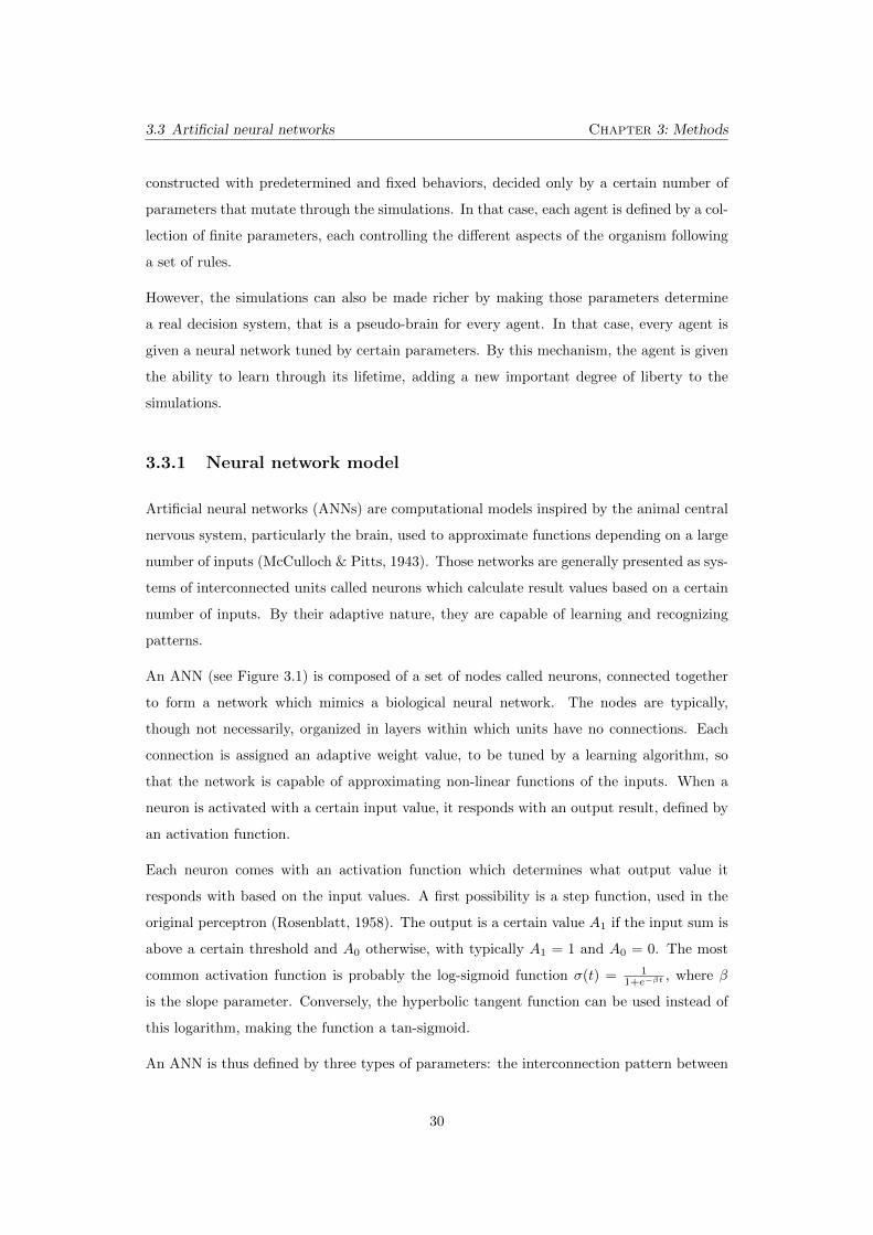
3.3 Artificial neural networks Chapter 3: Methods
constructed with predetermined and fixed behaviors, decided only by a certain number of
parameters that mutate through the simulations. In that case, each agent is defined by a col-
lection of finite parameters, each controlling the di↵erent aspects of the organism following
a set of rules.
However, the simulations can also be made richer by making those parameters determine
a real decision system, that is a pseudo-brain for every agent. In that case, every agent is
given a neural network tuned by certain parameters. By this mechanism, the agent is given
the ability to learn through its lifetime, adding a new important degree of liberty to the
simulations.
3.3.1 Neural network model
Artificial neural networks (ANNs) are computational models inspired by the animal central
nervous system, particularly the brain, used to approximate functions depending on a large
number of inputs (McCulloch & Pitts, 1943). Those networks are generally presented as sys-
tems of interconnected units called neurons which calculate result values based on a certain
number of inputs. By their adaptive nature, they are capable of learning and recognizing
patterns.
An ANN (see Figure 3.1) is composed of a set of nodes called neurons, connected together
to form a network which mimics a biological neural network. The nodes are typically,
though not necessarily, organized in layers within which units have no connections. Each
connection is assigned an adaptive weight value, to be tuned by a learning algorithm, so
that the network is capable of approximating non-linear functions of the inputs. When a
neuron is activated with a certain input value, it responds with an output result, defined by
an activation function.
Each neuron comes with an activation function which determines what output value it
responds with based on the input values. A first possibility is a step function, used in the
original perceptron (Rosenblatt, 1958). The output is a certain value A1
if the input sum is
above a certain threshold and A0
otherwise, with typically A1
= 1 and A0
= 0. The most
common activation function is probably the log-sigmoid function �(t) = 1
1+e��t , where �
is the slope parameter. Conversely, the hyperbolic tangent function can be used instead of
this logarithm, making the function a tan-sigmoid.
An ANN is thus defined by three types of parameters: the interconnection pattern between
30
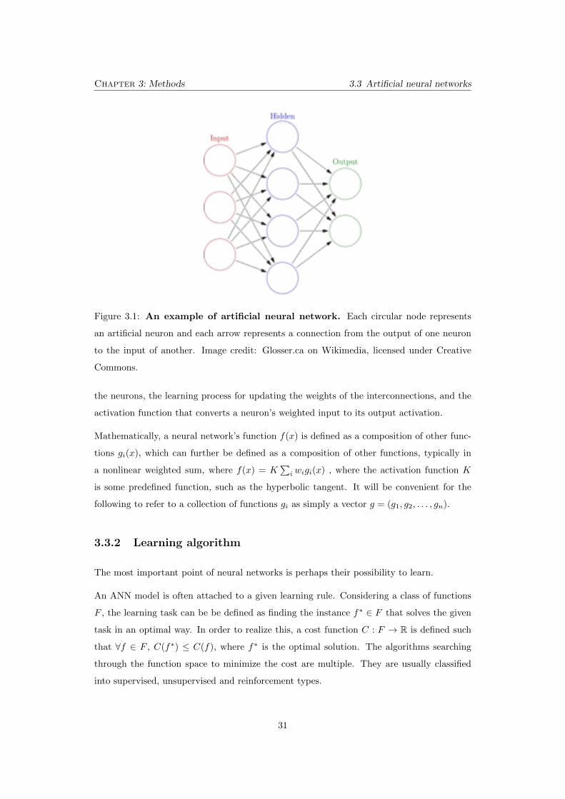
Chapter 3: Methods 3.3 Artificial neural networks
Figure 3.1: An example of artificial neural network. Each circular node represents
an artificial neuron and each arrow represents a connection from the output of one neuron
to the input of another. Image credit: Glosser.ca on Wikimedia, licensed under Creative
Commons.
the neurons, the learning process for updating the weights of the interconnections, and the
activation function that converts a neuron’s weighted input to its output activation.
Mathematically, a neural network’s function f(x) is defined as a composition of other func-
tions gi(x), which can further be defined as a composition of other functions, typically in
a nonlinear weighted sum, where f(x) = KP
i wigi(x) , where the activation function K
is some predefined function, such as the hyperbolic tangent. It will be convenient for the
following to refer to a collection of functions gi as simply a vector g = (g1
, g2
, . . . , gn).
3.3.2 Learning algorithm
The most important point of neural networks is perhaps their possibility to learn.
An ANN model is often attached to a given learning rule. Considering a class of functions
F , the learning task can be be defined as finding the instance f⇤ 2 F that solves the given
task in an optimal way. In order to realize this, a cost function C : F ! R is defined such
that 8f 2 F , C(f⇤) C(f), where f⇤ is the optimal solution. The algorithms searching
through the function space to minimize the cost are multiple. They are usually classified
into supervised, unsupervised and reinforcement types.
31
3.3 Artificial neural networks Chapter 3: Methods
In supervised learning, the goal is to infer a mapping function from a set of examples i.e.
find a function f : X ! Y 2 F that matches given pairs (x, y), with x 2 X and y 2 Y .
In this case, the cost function must be a measure of the error between a tentative mapping
and the data. This method, though e�cient, is only applicable to problems with available
knowledge of the result requirements and constraints.
A common algorithm is based on minimizing the average squared error MSE = 1
n
Pni=1
(fi(x)�
yi)2 where f(x) is the network’s output vector and y is the vector of target values from the
example pairs, which can be done using gradient descent. This method is called back-
propagation, and is usual in training the so-called multilayer-perceptron neural networks.
Supervised learning usually applies though is not limited to pattern and sequence recognition
tasks.
For unsupervised learning, some data x is given and the cost function C(x, f(x)) to be min-
imized, which is dependent on the task. Usual applications of this paradigm are clustering,
classification and compression.
In the case of reinforcement learning, the data is not directly presented to the learning
system, but rather is obtained by interactions with an environment so as to maximize some
cumulative reward. Reinforcement methods apply particularly well to complex search spaces
where classical approaches would be intractable since they require prior knowledge about the
MDP. A typical reinforcement learning model, based on Markov decision processes (MDP),
consists of a set of environment states S, a set of actions A, a number of rules of transition
between states, a description of the agent’s input data and a reward function for each
transition (Howard, 1960). To avoid wasting resources on exploring search spaces that are
often considerably large, this approach can benefit from clever exploration mechanisms.
3.3.3 Search space exploration
A purely random exploration of the search space is obviously not an acceptable strategy to
find an optimum. To attain a good performance, it is necessary to plan a search following
an e�cient schedule or adaptively based on a heuristic. The search is then said to follow a
policy, that is a mapping assigning a certain probability distribution over the directions to
all possible histories of search.
In case structural aspects of the space are known or can be learned online during the search,
the algorithm can avoid brute forcing by biasing the search towards more likely directions,
32
Chapter 3: Methods 3.3 Artificial neural networks
for example at the very least by implementing gradient descent on the data. The search
can indeed without any loss of generality be restricted to the set of the so-called stationary
policies, which depend only on the last state visited.
Nevertheless, policy search methods may converge slowly because of noisy information.
Alternatives include fully or partly gradient-free algorithms, such as simulated annealing,
cross-entropy search or methods of evolutionary computation (Deisenroth et al., 2013). The
approaches chosen in this thesis is derived from the latter one.
Evolutionary computation uses pseudo-genomes representing artificial neural networks by
describing, directly or indirectly, their connectivity structure and weights. Further details
about evolutionary algorithms are explicited in section 3.4.
The problem of convergence depends on di↵erent factors, notably the presence of local min-
ima, the dependency on initial conditions, and the scalability on input data or parameters.
3.3.4 Network architectures
In a neural network, the first neurons that receive information directly from the environment
form the input layer. The neurons that produce the resulting data processed by the network
constitute the output layer. Layers between the input and the output layer are called hidden
layers. Based on the connectivity in place between the input and the output, neural networks
are able to process and store various amounts and complexities of information. The number
of hidden units and the architecture of the network they form determine the capacity, that
is the ability of the system to model any given function.
The number of neurons present in the hidden layer is one of the main factors influencing
the capacity. More hidden layers can make the system more robust and flexible to the
learning. However, this power comes with a more costly training algorithm because the
overspecification can make generalization di�cult.
The simplest architecture is the feedforward network (see Figure 3.1, represented by a di-
rected acyclic graph of processing units. In this case, the di↵erent layers of neurons are just
receiving their input from the previous layer, and outputting the processed result to the
next one, without any feedback. Formally, this means that the weights from a neuron to an-
other neuron in a previous layer is zero, as well as the weights from the units to themselves.
A feedforward network with nonlinear activation functions and using backpropagation (see
section 3.3.2) is called a multilayer perceptron (MLP), and is able to classify non linearly
33
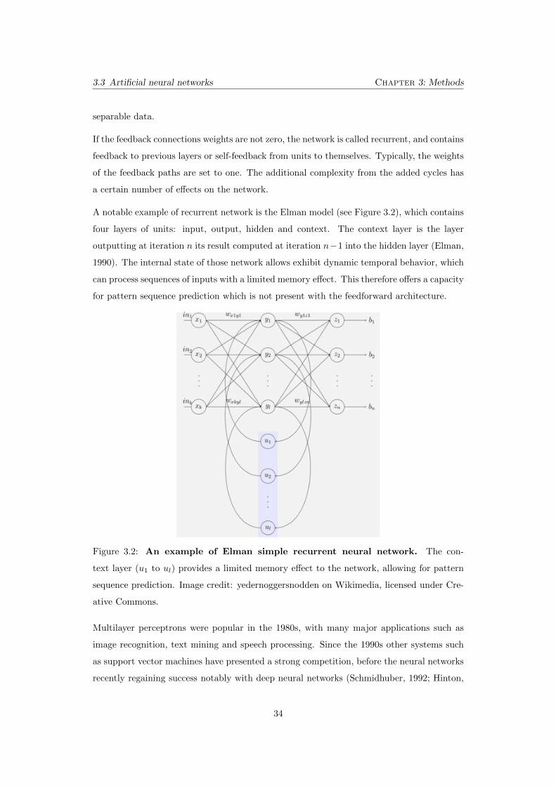
3.3 Artificial neural networks Chapter 3: Methods
separable data.
If the feedback connections weights are not zero, the network is called recurrent, and contains
feedback to previous layers or self-feedback from units to themselves. Typically, the weights
of the feedback paths are set to one. The additional complexity from the added cycles has
a certain number of e↵ects on the network.
A notable example of recurrent network is the Elman model (see Figure 3.2), which contains
four layers of units: input, output, hidden and context. The context layer is the layer
outputting at iteration n its result computed at iteration n�1 into the hidden layer (Elman,
1990). The internal state of those network allows exhibit dynamic temporal behavior, which
can process sequences of inputs with a limited memory e↵ect. This therefore o↵ers a capacity
for pattern sequence prediction which is not present with the feedforward architecture.
Figure 3.2: An example of Elman simple recurrent neural network. The con-
text layer (u1
to ul) provides a limited memory e↵ect to the network, allowing for pattern
sequence prediction. Image credit: yedernoggersnodden on Wikimedia, licensed under Cre-
ative Commons.
Multilayer perceptrons were popular in the 1980s, with many major applications such as
image recognition, text mining and speech processing. Since the 1990s other systems such
as support vector machines have presented a strong competition, before the neural networks
recently regaining success notably with deep neural networks (Schmidhuber, 1992; Hinton,
34
Chapter 3: Methods 3.4 Neuroevolution
2007).
3.4 Neuroevolution
Evolution is central to the study of living systems. A way to include this aspect in artificial
life models is to add a natural selection process in them. In this section, we review the
details of genetic algorithms and their application to the evolution of neural networks, a
very common approach in robotics and artificial life.
3.4.1 Evolutionary algorithms
Natural selection can be thought as an optimization process that searches through a set of
possible individuals, in order to find those with the highest fitness. Fisher (1958) founded
mathematical genetics by viewing the chromosome as a string of genes and providing a
mathematical formula specifying the rate at which particular genes would spread through
a population. Holland (1995) later generalized this concept, creating the genetic algorithm
(GA), which is a generalized, computer-executable version of Fisher’s formulation.
A genetic algorithm emulates the process of evolution and natural selection, including fitness
evaluation, selection process, and descent with modification. The fitness evaluates each
individual in the current population with a value characterizing its level of performance
at a task. The selection process picks the best performing individuals to reproduce into
the next generation of artificial brains. Finally, the descent with modification updates the
current population by removing previous individuals and generating the o↵spring of the ones
previously selected, by creating copies of their parents with slight modifications.
3.4.2 Selection methods
Genetic algorithms use di↵erent methods to select the potentially good solutions among the
individuals present in the population, after each one has been assigned a fitness value. Two
largely used selection methods are the roulette wheel and tournament selection.
The roulette wheel selection proceeds by using the fitness values to associate a probability of
selection to each individual. The selection is based proportionally on each individual’s fitness
f . The probability of an individual i in the population of n members is pi = fiPnj=1 fj
. As a
35
3.4 Neuroevolution Chapter 3: Methods
result, candidates with a higher fitness will be more likely to be selected, without removing
the possibility for them to be rejected, unlike methods such as truncation selection, which
eliminate a fixed percentage of the weakest candidates. Previously executed in O(logn), this
algorithm has recently been implemented in O(1) by picking an individual choosing it for
selection with probability fifM
, where fM is the maximum fitness in the population (Lipowski
& Lipowska, 2012).
A variant of the roulette wheel consists in choosing several individuals from the population
by repeated random sampling, with a single random value to sample all of the solutions
by choosing them at evenly spaced intervals, thus giving individual with a weaker fitness a
better chance to be chosen. This method is called stochastic universal selection, and removes
an unfair bias from the roulette wheel method, by avoiding the fittest members to saturate
the candidate space (Baker, 1987). This selection method will be used in most of the studies
presented in the following chapters of this thesis.
Another method is tournament selection, which implies running several tournament tests
among a few individuals chosen at random from the population, assigning them di↵erent
fitnesses. The winner of each tournament, with the best fitness, is usually selected for
crossover. But a variant of the method may also include them all in the mix, with their
respective cumulative assigned fitness. The selection pressure can be adjusted by changing
the tournament size. This selection method will be used in one simulation setup of Chapter
6.
A usual variant called elitist selection consists in taking the best individuals in a generation
unchanged in the next generation. Another variant is based on a cut-o↵ value for the fitness,
getting rid of every value under a given threshold.
All the methods presented above are reward-based, which means the probability for an indi-
vidual to be selected is proportional to the cumulative reward, obtained by each individual
during its lifetime.
Once a subset of fit individuals has been selected, there are several ways to generate the
individuals to add to the next population. A single crossover point on both parents’ organism
strings is selected. All data beyond that point in either organism string is swapped between
the two parent organisms (Haynes & Sen, 1997). Two-point crossover calls for two points to
be selected on the parent organism strings. Everything between the two points is swapped
between the parent organisms (Eiben & Smith, 2003). Another crossover variant, the so-
called cut and splice approach, results in a change in length of the children strings. The
36
Chapter 3: Methods 3.4 Neuroevolution
reason for this di↵erence is that each parent string has a separate choice of crossover point.
3.4.3 Evolving neural networks
Neuroevolution is machine learning that uses evolutionary algorithms to train artificial neu-
ral networks.
While supervised learning algorithms require to gather a database of correct input-output
pairs to train the system on, neuroevolution is fine with only a measure of a network’s
performance at a task, as mentioned in section 3.3.2.
This concept is commonly applied in the study of computer games, where the result of a
game can be obtained from iterating a given strategy until the ending conditions are met.
The stretch is not hard to imagine from those games to a more general type of game that
would involve an agent embodied in an environment, whose decisions would decide for its
survival. The system is evidently a metaphorically relevant system for the study of living
creatures, in biology or evolutionary robotics, not only because of that intuitive stretch, but
also for its multiple inherent qualities.
In neuroevolution, genotypes are mapped to neural network phenotypes by a direct or in-
direct encoding scheme. The produced networks are then evaluated according to a fitness
function corresponding to a given task they need to perform. In direct encoding schemes,
the genotypes directly map to the phenotypes, in the sense that every element, neuron or
connection, of the neural network is specified explicitly inside the genotype. In the case
of an indirect encoding, the genotype specifies only indirectly how that network should be
generated, so as to allow for recurring features, to reduce the genotype search space or to
better map the genotype to the problem domain.
A notable example of neuroevolution algorithm is NEAT (Stanley & Miikkulainen, 2002),
which evolves both the weights and the structures of the artificial neural networks, so as to
balance between the fitness of evolved solutions and their diversity. The method is based on
tracking genes with history markers to allow crossover among topologies, applying speciation
to preserve innovations, and incrementally developing more and more complex topologies.
NEAT performs particularly well compared to other methods, and has been extended to
many more specialized methods, notably HyperNEAT (Stanley, 2006) which is aimed for
large-scale networks and using compositional pattern producing networks (CPPN).
37
3.4 Neuroevolution Chapter 3: Methods
3.4.4 Neuroevolution in artificial life
Neuroevolution is commonly used in the field of artificial life, by mixing evolutionary and
learning techniques. This type of approach is motivated by the fact that learning can
enhance the adaptive power of evolution (Nolfi & Parisi, 1993). Combining ANNs with EAs
for adapting agent behavior has recently received significant research attention (Floreano
et al., 2007; Mitri et al., 2009b).
In artificial life studies, as mentioned in Section 3.1, agents are controlled by fixed neural
network controllers. The behavior of the agents can benefit from the combination of learning
techniques with the neuroevolution of the controllers. The algorithm gradually improves the
agents’ performance on tasks such as pattern matching or foraging for a resource in a spatial
environment.
Examples of such studies involving neuroevolution and embodied agents, have been intro-
duced in Sections 3.1.3 and 3.1. More references will be contextually given in the following
chapters, when comparing the literature’s model to our own.
38
Chapter4Signal-based coordination and neutral se-
lection
Since Reynold’s boids, coordinated motion has often been reproduced in number of artifi-
cial models, but the conditions leading to its emergence are still subject to research, with
candidates ranging from obstacle avoidance to virtual leaders. The relation of spatial co-
ordination and group cooperation has long been studied in game theory and evolutionary
biology.
This chapter presents a model of simulated agents moving in a three-dimensional environ-
ment. Their movements are controlled by artificial networks, evolved through generations
of an asynchronous selection algorithm, at the term of which the agents become able to
produce cooperative, coordinated behavior.
We present results in which individuals develop swarming using only their ability to listen
to each other’s signals. The agents are selected based on their performance at finding
invisible resources in space giving them fitness. The agents are shown to use the information
exchanged between them via signaling to form temporary leader-follower relations allowing
them to flock together. The swarmers outperform the non-swarmers at finding the resource,
thus reaching a neutral evolutionary space which leads to a genetic drift.
4.1 Swarming behavior
The ability of fish schools, insect swarms or starling murmurations (Figure 4.1) to shift shape
as one and coordinate their motion in space has been studied extensively because of their
implications for the evolution of social cognition, collective animal behavior and artificial
life (Couzin, 2009).
39
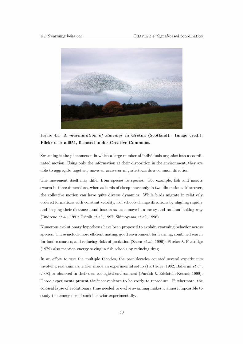
4.1 Swarming behavior Chapter 4: Signal-based coordination
Figure 4.1: A murmuration of starlings in Gretna (Scotland). Image credit:
Flickr user ad551, licensed under Creative Commons.
Swarming is the phenomenon in which a large number of individuals organize into a coordi-
nated motion. Using only the information at their disposition in the environment, they are
able to aggregate together, move en masse or migrate towards a common direction.
The movement itself may di↵er from species to species. For example, fish and insects
swarm in three dimensions, whereas herds of sheep move only in two dimensions. Moreover,
the collective motion can have quite diverse dynamics. While birds migrate in relatively
ordered formations with constant velocity, fish schools change directions by aligning rapidly
and keeping their distances, and insects swarms move in a messy and random-looking way
(Budrene et al., 1991; Czirok et al., 1997; Shimoyama et al., 1996).
Numerous evolutionary hypotheses have been proposed to explain swarming behavior across
species. These include more e�cient mating, good environment for learning, combined search
for food resources, and reducing risks of predation (Zaera et al., 1996). Pitcher & Partridge
(1979) also mention energy saving in fish schools by reducing drag.
In an e↵ort to test the multiple theories, the past decades counted several experiments
involving real animals, either inside an experimental setup (Partridge, 1982; Ballerini et al.,
2008) or observed in their own ecological environment (Parrish & Edelstein-Keshet, 1999).
Those experiments present the inconvenience to be costly to reproduce. Furthermore, the
colossal lapse of evolutionary time needed to evolve swarming makes it almost impossible to
study the emergence of such behavior experimentally.
40
Chapter 4: Signal-based coordination 4.1 Swarming behavior
Computer modeling has recently provided researchers with new, easier ways to test hypothe-
ses on collective behavior. As mentioned in Section 3.1, simulating individuals on machines
o↵ers easy modification of setup conditions and parameters, tremendous data generation,
full reproducibility of every experiment, and easier identification of the underlying dynamics
of complex phenomena.
4.1.1 From Reynolds’ boids to recent approaches
In a massively cited paper, Reynolds (1987) introduces the boids model simulating 3D swarm-
ing of agents called boids controlled only by three simple rules:
• Alignment : move in the same direction as neighbours
• Cohesion: Remain close to neighbours
• Separation: Avoid collisions with neighbours
Various works have since then reproduced swarming behavior, often by the means of an
explicitly coded set of rules. For instance, Mataric (1992) proposes a generalization of
Reynolds’ original model with an optimally weighted combination of six basic interaction
primitives1. Hartman & Benes (2006) come up with yet another variant of the original
model, by adding a complementary force to the alignment rule, that they call change of
leadership. Unfortunately, in spite of the insight this kind of approach brings into the
dynamics of swarming, it shows little about the pressures leading to its emergence. Many
other approaches are based on informed agents or fixed leaders (Cucker & Huepe, 2008; Su
et al., 2009; Yu et al., 2010).
For that reason, experimenters attempted to simulate swarming without a fixed set of rules,
rather by incorporating into each agent an artificial neural network brain that controls its
movements. The swarming behavior is evolved by copy with mutations of the chromosomes
encoding the neural network parameters. By comparing the impact of di↵erent selective
pressures, this type of methodology, first used in Eberhart & Kennedy (1995) to solve
optimization problems, eventually allowed to study the evolutionary emergence of swarming.
Tu & Terzopoulos (1994) have swarming emerge from the application of artificial pressures
consisting of hunger, libido and fear. Other experimenters have analyzed prey/predator
systems to show the importance of sensory system and predator confusion in the evolution
1Namely, those primitives are collision avoidance, following, dispersion, aggregation, homing and flocking.
41
4.1 Swarming behavior Chapter 4: Signal-based coordination
of swarming in preys (Ward et al., 2001; Olson et al., 2013).
In spite of many pressures hypothesized to produce swarming behavior, designed setups
presented in the literature are often complex and specific. Previous works typically introduce
models with very specific environments, where agents are given specialized sensors designed
to be more sensitive to a particular type of inputs. While they are bringing valuable results
to the community, one may wonder about systems with a simpler, more general design.
In addition, even when studies focus on fish or insects that swarm in 3D (Ward et al., 2001)
most keep their model in 2D. While the swarming can be considered to be similar in most
cases, the mapping from 2D to 3D is found to be non-trivial (Sayama, 2012). Indeed, the
addition of a third degree of freedom may enable agents to produce significantly distinct
and more complex behaviors.
4.1.2 Signaling agents in a resource finding task
This work studies the emergence of swarming in a population of agents using a basic signaling
system, while performing a simple resource gathering task.
Simulated agents move around in a three dimensional space, looking for a vital but invisible
food resource randomly distributed in the environment. The agents are emitting signals
that can be perceived by other individuals’ sensors within a certain radius. Both agent’s
motion and signaling are controlled by an artificial neural network embedded in each agent,
evolved over time by an asynchronous genetic algorithm. Agents that consume enough food
are enabled to reproduce, whereas those whose energy drops to zero are removed from the
simulation.
Each experiment is performed in two steps: training the agents in an environment with
resource locations providing fitness, then testing in an environment without fitness.
During the training, we observe that the agents progressively come to coordinate into clus-
tered formations. That behavior is then preserved in the second step. Such patterns do not
appear in control experiments having the simulation start directly from the second phase,
with the absence of resource locations. If at any point the signaling is switched o↵, the
agents immediately break the swarming formation. A swarming behavior is only observed
once the communication is turned back on. Furthermore, the simulations with signaling
lead to agents gathering very closely around food patches, whereas control simulations with
silenced agents end up with all individuals wandering around erratically.
42
Chapter 4: Signal-based coordination 4.2 Asynchronous agent-based simulation
The main contribution of this work is to show that collective motion can originate, without
explicit central coordination, from the combination of a generic communication system and
a simple resource gathering task. As a secondary contribution, our model also demonstrates
how swarming behavior can lead to a neutral evolutionary space, where no more selection
is applied on the gene pool.
A specific genetic algorithm with an asynchronous reproduction scheme is developed and
used to evolve the agents’ neural controllers. In addition, the search for resource is shown
to improve from the agents clustering, eventually leading to the agents gathering closely
around goal areas. An in-depth analysis shows increasing information transfer between
agents throughout the learning phase, and the development of leader/follower relations that
eventually push the agents to organize into clustered formations.
4.2 Asynchronous agent-based simulation
4.2.1 Agents in a 3D world
We simulate a group of agents moving around in a cubic, toroidal arena of 600⇥ 600⇥ 600.
The agents rely on energy to survive. If at any point an agent’s energy drops to zero, it
is immediately removed from the environment. The task for the agents is to get as close
as possible to a preset resource spot. By getting close to one of those spots, agents can
gain more energy, allowing them to counterbalance the energy losses due to movement and
signaling. An agent whose energy drops to zero is removed from the simulation. In this
regard, the energy also represents each agent’s fitness, and in this work both terms are used
interchangeably.
The agent’s position is determined by three floating point coordinates between 0.0 and 600.0.
Each agent is positioned randomly at the start of the simulation, and then moves at a fixed
speed of 1 unit per iteration. Every iteration, the agent’s new velocity ~ct is obtained by
rotating its velocity vector at the previous time step ~ct�1
by two Euler angles: for the
agent’s pitch (i.e. elevation) and ✓ for the agent’s yaw (i.e. heading). The rotation is
determined by the two motor output values of the neural controller o1
and o2, determining
respectively the acceleration in y and z in the agent’s inertial frame of reference, while the
norm of the velocity is kept constant. The agent’s position ~xt is then updated according to
its current velocity with ~xt = ~xt�1
+ ~ct.
43
4.2 Asynchronous agent-based simulation Chapter 4: Signal-based coordination
4.2.2 Communication among agents
Every agent is also provided with one communication actuator capable of sending signals
with intensities (signals are encoded as floating point values ranging from 0.0 to 1.0), and
six communication sensors allowing it to detect signals produced by other agents up to a
distance of 100 from 6 directions, namely frontal (0, 1, 0), rear (0,�1, 0), left (1, 0, 0), right
(�1, 0, 0), top (0, 0, 1) and bottom (0, 0,�1)). The communication sensors are implemented
so that every source point in a 100-radius sphere around the agent is linked to one and
only one of its sensors. The distance to the source proportionally a↵ects the intensity of a
received signal, and signals from agents above a 100 distance are ignored. The sensor whose
direction is the closest to the signaling source receives one float value, equal to the sum of
every signal emitted within range, divided by the distance, and normalized between 0 and
1.
4.2.3 Agents controlled by neural networks
The agent’s neural controller is implemented by a modified Elman artificial neural network
with 6 input neurons, encoding the activation states of the corresponding 6 sensors, fully
connected through a 10-neuron hidden layer to 3 output neurons controlling the two motors
and the communication signal emitted by the agent. The hidden layer is given a form of
memory feedback from a 10-neuron context layer, containing the values of the hidden layer
from the previous time step.
All nodes in the neural network take input values between 0 and 1. All output values are also
floating values between 0 and 1, the motor outputs are then converted to angles between �⇡
to ⇡. The activation state of internal neurons is updated according to a sigmoid function.
The weights of each connection in the neural network, comprised between 0 and 1, are stored
in an array. That array, constituting the agent’s genotype, is then evolved using a specific
genetic algorithm described below.
4.2.4 An asynchronous reproduction scheme
Genetic algorithms (Fraser, 1960; Bremermann, 1962; John, 1992), inspired by Darwin’s
principle of natural evolution (cf. Section 2.1), simulate the descent with modification of
a population of chromosomes, selected generation through generation by a defined fitness
44
Chapter 4: Signal-based coordination 4.2 Asynchronous agent-based simulation
function.
Our model di↵ers from the usual genetic algorithm paradigm (cf. Section 3.4), in that
it designs variation and selection in an asynchronous way. The reproduction takes place
continuously throughout the simulation, creating overlapping generations of agents. This
allows for a more natural, continuous model, as no global clock is defined, that could bias
or weaken the model.
Every new agent is born with an energy equal to 2.0. In the course of the simulation, each
agent can gain or lose a variable amount of energy. At iteration t, the fitness function fi for
agent i is defined by fi(t) = rdi(t)
where r is the reward value and di is the agent’s distance to
the goal. The reward value is controlled by the simulation such that the population remains
between 100 and 500 agents. All the way through the simulation, the agents also spend a
fixed amount of energy for movement (0.01 per iteration) and a variable amount of energy
for signaling costs (0.001 ⇥ signal intensity per iteration).
The weights of every connection in the neural network (apart from the links from hidden
to context nodes, which have fixed weights) are encoded in genotypes and evolved through
successive generations of agents. Each weight is represented by a unique floating point value
in the genotype vector, such that the size of the vector corresponds to the total number of
connections in a neural network. The simulation uses a genetic algorithm with overlapping
generations to evolve the weights of the neural networks. Whenever an agent accumulates
10.0 in energy, a replica of itself (with a 5% mutation in the genotype) is created and added
to a random position in the arena. The agent’s energy is decreased by 8.0 and the new
replica’s energy is set to 2.0. The choice for random initial positions is to avoid biasing the
proximity of agents, so that reproduction does not become a way for agents to create local
clusters.
Indeed, a local reproduction scheme (i.e. giving birth to o↵spring close to their parents) leads
rapidly to an explosion in population size, as the agents that are close to the resource create
many o↵spring that will be very fit too, thus able to replicate very fast as well. This is why
the newborn o↵spring is placed randomly in the environment. On a side note, population
bursts occur solely when the neighborhood radius is small (under 10), while values over 100
do not lead to population bursts.
For the genetic algorithm to be e↵ective, the number of agents must be maintained above
a certain level. Also, the computation power limits the population size. The fitness allowed
to the agents is therefore adjusted in order to maintain an ideal number as close as possible
45
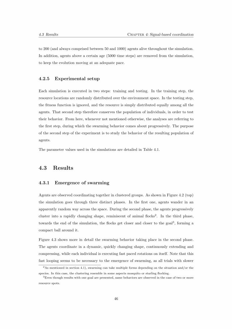
4.3 Results Chapter 4: Signal-based coordination
to 200 (and always comprised between 50 and 1000) agents alive throughout the simulation.
In addition, agents above a certain age (5000 time steps) are removed from the simulation,
to keep the evolution moving at an adequate pace.
4.2.5 Experimental setup
Each simulation is executed in two steps: training and testing. In the training step, the
resource locations are randomly distributed over the environment space. In the testing step,
the fitness function is ignored, and the resource is simply distributed equally among all the
agents. That second step therefore conserves the population of individuals, in order to test
their behavior. From here, whenever not mentioned otherwise, the analyses are referring to
the first step, during which the swarming behavior comes about progressively. The purpose
of the second step of the experiment is to study the behavior of the resulting population of
agents.
The parameter values used in the simulations are detailed in Table 4.1.
4.3 Results
4.3.1 Emergence of swarming
Agents are observed coordinating together in clustered groups. As shown in Figure 4.2 (top)
the simulation goes through three distinct phases. In the first one, agents wander in an
apparently random way across the space. During the second phase, the agents progressively
cluster into a rapidly changing shape, reminiscent of animal flocks2. In the third phase,
towards the end of the simulation, the flocks get closer and closer to the goal3, forming a
compact ball around it.
Figure 4.3 shows more in detail the swarming behavior taking place in the second phase.
The agents coordinate in a dynamic, quickly changing shape, continuously extending and
compressing, while each individual is executing fast paced rotations on itself. Note that this
fast looping seems to be necessary to the emergence of swarming, as all trials with slower
2As mentioned in section 4.1), swarming can take multiple forms depending on the situation and/or the
species. In this case, the clustering resemble in some aspects mosquito or starling flocking.3Even though results with one goal are presented, same behaviors are observed in the case of two or more
resource spots.
46
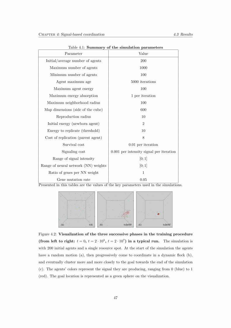
Chapter 4: Signal-based coordination 4.3 Results
Table 4.1: Summary of the simulation parameters
Parameter Value
Initial/average number of agents 200
Maximum number of agents 1000
Minimum number of agents 100
Agent maximum age 5000 iterations
Maximum agent energy 100
Maximum energy absorption 1 per iteration
Maximum neighborhood radius 100
Map dimensions (side of the cube) 600
Reproduction radius 10
Initial energy (newborn agent) 2
Energy to replicate (threshold) 10
Cost of replication (parent agent) 8
Survival cost 0.01 per iteration
Signaling cost 0.001 per intensity signal per iteration
Range of signal intensity [0; 1]
Range of neural network (NN) weights [0; 1]
Ratio of genes per NN weight 1
Gene mutation rate 0.05
Presented in this tables are the values of the key parameters used in the simulations.
Figure 4.2: Visualization of the three successive phases in the training procedure
(from left to right: t = 0, t = 2 · 105, t = 2 · 107) in a typical run. The simulation is
with 200 initial agents and a single resource spot. At the start of the simulation the agents
have a random motion (a), then progressively come to coordinate in a dynamic flock (b),
and eventually cluster more and more closely to the goal towards the end of the simulation
(c). The agents’ colors represent the signal they are producing, ranging from 0 (blue) to 1
(red). The goal location is represented as a green sphere on the visualization.
47
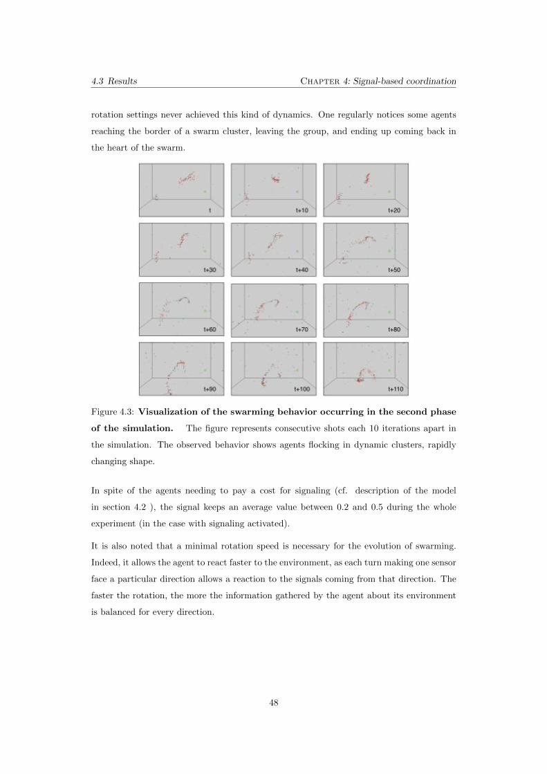
4.3 Results Chapter 4: Signal-based coordination
rotation settings never achieved this kind of dynamics. One regularly notices some agents
reaching the border of a swarm cluster, leaving the group, and ending up coming back in
the heart of the swarm.
Figure 4.3: Visualization of the swarming behavior occurring in the second phase
of the simulation. The figure represents consecutive shots each 10 iterations apart in
the simulation. The observed behavior shows agents flocking in dynamic clusters, rapidly
changing shape.
In spite of the agents needing to pay a cost for signaling (cf. description of the model
in section 4.2 ), the signal keeps an average value between 0.2 and 0.5 during the whole
experiment (in the case with signaling activated).
It is also noted that a minimal rotation speed is necessary for the evolution of swarming.
Indeed, it allows the agent to react faster to the environment, as each turn making one sensor
face a particular direction allows a reaction to the signals coming from that direction. The
faster the rotation, the more the information gathered by the agent about its environment
is balanced for every direction.
48
Chapter 4: Signal-based coordination 4.3 Results
4.3.2 Neighborhood
We choose to measure swarming behavior in agents by looking at the average number of
neighbors within a radius of 100 distance around each agent. Figure 4.4 shows the evolution
of the average number of neighbors, over 10 di↵erent runs, respectively with signaling turned
on and o↵. A much higher value is reached around time step 105 in the signaling case, while
the value remains for the silent control. The swarming emerges only with the signaling
switched on, and as soon as the signaling is silenced, the agents rapidly stop their swarming
behavior and start wandering randomly in space.
0 2 4 6 8 10 12
x 105
0
0.05
0.1
0.15
0.2
0.25
0.3
0.35
0.4
0.45
0.5
Time steps
Ave
rag
e n
um
be
r o
f n
eig
hb
ors
Average number of neighbors (10 runs) with signalling ON vs OFF
signalling ON
signalling OFF
Figure 4.4: Comparison of the average number of neighbors (average over 10 runs,
with 106 iterations) in the case signaling is turned on versus o↵.
We also want to measure the influence of each agent on its neighborhood. To do so, the
inward average transfer entropy on agent’s velocities is calculated4 between each neighbor
within a distance of 100 and the agent itself. We will refer to this measure as inward
neighborhood transfer entropy (NTE). This can be considered a measure of how much the
agents are “following” their neighbors at a given time step. The values rapidly take o↵ on
the regular simulation (with signaling switched on), while they remain low for the silent
control, as we can see for example in Figure 4.5.
Similarly, we can calculate the outward neighborhood transfer entropy (i.e. the average
transfer entropy from an agent to its neighbors). We may look at the evolution of this value
through the simulation, in an attempt to capture the apparition of local leaders in the swarm
clusters. Even though the notion of leadership is hard to define, the study of the flow of
information is essential in the study of swarms. The single individuals’ outward NTE shows
4The calculations are analogous to Wibral et al. (2013).
49
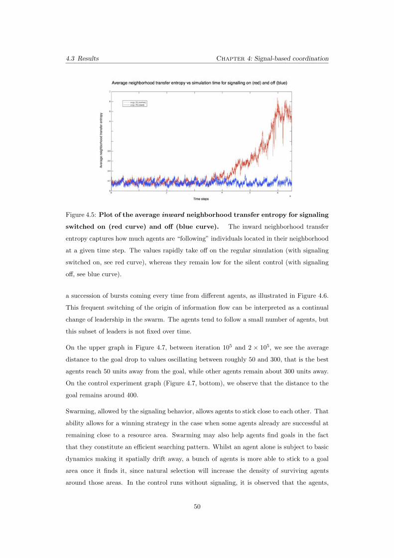
4.3 Results Chapter 4: Signal-based coordination
Figure 4.5: Plot of the average inward neighborhood transfer entropy for signaling
switched on (red curve) and o↵ (blue curve). The inward neighborhood transfer
entropy captures how much agents are “following” individuals located in their neighborhood
at a given time step. The values rapidly take o↵ on the regular simulation (with signaling
switched on, see red curve), whereas they remain low for the silent control (with signaling
o↵, see blue curve).
a succession of bursts coming every time from di↵erent agents, as illustrated in Figure 4.6.
This frequent switching of the origin of information flow can be interpreted as a continual
change of leadership in the swarm. The agents tend to follow a small number of agents, but
this subset of leaders is not fixed over time.
On the upper graph in Figure 4.7, between iteration 105 and 2 ⇥ 105, we see the average
distance to the goal drop to values oscillating between roughly 50 and 300, that is the best
agents reach 50 units away from the goal, while other agents remain about 300 units away.
On the control experiment graph (Figure 4.7, bottom), we observe that the distance to the
goal remains around 400.
Swarming, allowed by the signaling behavior, allows agents to stick close to each other. That
ability allows for a winning strategy in the case when some agents already are successful at
remaining close to a resource area. Swarming may also help agents find goals in the fact
that they constitute an e�cient searching pattern. Whilst an agent alone is subject to basic
dynamics making it spatially drift away, a bunch of agents is more able to stick to a goal
area once it finds it, since natural selection will increase the density of surviving agents
around those areas. In the control runs without signaling, it is observed that the agents,
50
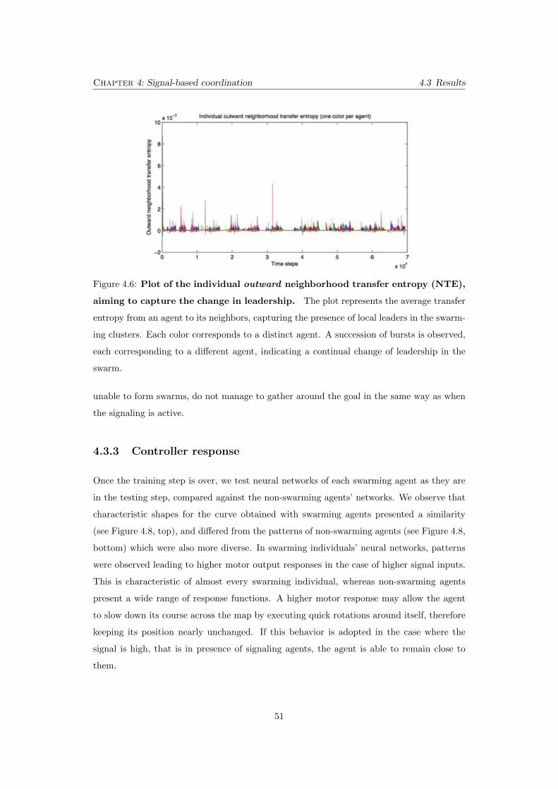
Chapter 4: Signal-based coordination 4.3 Results
Figure 4.6: Plot of the individual outward neighborhood transfer entropy (NTE),
aiming to capture the change in leadership. The plot represents the average transfer
entropy from an agent to its neighbors, capturing the presence of local leaders in the swarm-
ing clusters. Each color corresponds to a distinct agent. A succession of bursts is observed,
each corresponding to a di↵erent agent, indicating a continual change of leadership in the
swarm.
unable to form swarms, do not manage to gather around the goal in the same way as when
the signaling is active.
4.3.3 Controller response
Once the training step is over, we test neural networks of each swarming agent as they are
in the testing step, compared against the non-swarming agents’ networks. We observe that
characteristic shapes for the curve obtained with swarming agents presented a similarity
(see Figure 4.8, top), and di↵ered from the patterns of non-swarming agents (see Figure 4.8,
bottom) which were also more diverse. In swarming individuals’ neural networks, patterns
were observed leading to higher motor output responses in the case of higher signal inputs.
This is characteristic of almost every swarming individual, whereas non-swarming agents
present a wide range of response functions. A higher motor response may allow the agent
to slow down its course across the map by executing quick rotations around itself, therefore
keeping its position nearly unchanged. If this behavior is adopted in the case where the
signal is high, that is in presence of signaling agents, the agent is able to remain close to
them.
51
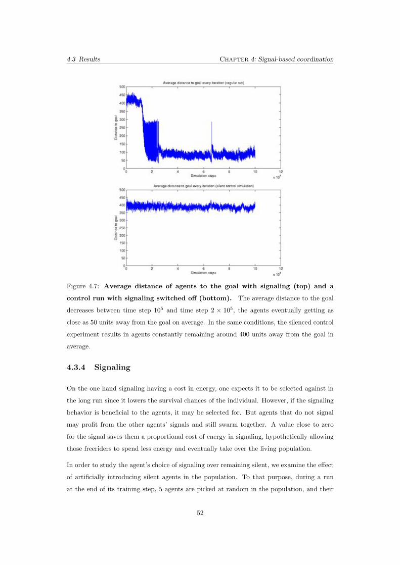
4.3 Results Chapter 4: Signal-based coordination
Figure 4.7: Average distance of agents to the goal with signaling (top) and a
control run with signaling switched o↵ (bottom). The average distance to the goal
decreases between time step 105 and time step 2 ⇥ 105, the agents eventually getting as
close as 50 units away from the goal on average. In the same conditions, the silenced control
experiment results in agents constantly remaining around 400 units away from the goal in
average.
4.3.4 Signaling
On the one hand signaling having a cost in energy, one expects it to be selected against in
the long run since it lowers the survival chances of the individual. However, if the signaling
behavior is beneficial to the agents, it may be selected for. But agents that do not signal
may profit from the other agents’ signals and still swarm together. A value close to zero
for the signal saves them a proportional cost of energy in signaling, hypothetically allowing
those freeriders to spend less energy and eventually take over the living population.
In order to study the agent’s choice of signaling over remaining silent, we examine the e↵ect
of artificially introducing silent agents in the population. To that purpose, during a run
at the end of its training step, 5 agents are picked at random in the population, and their
52
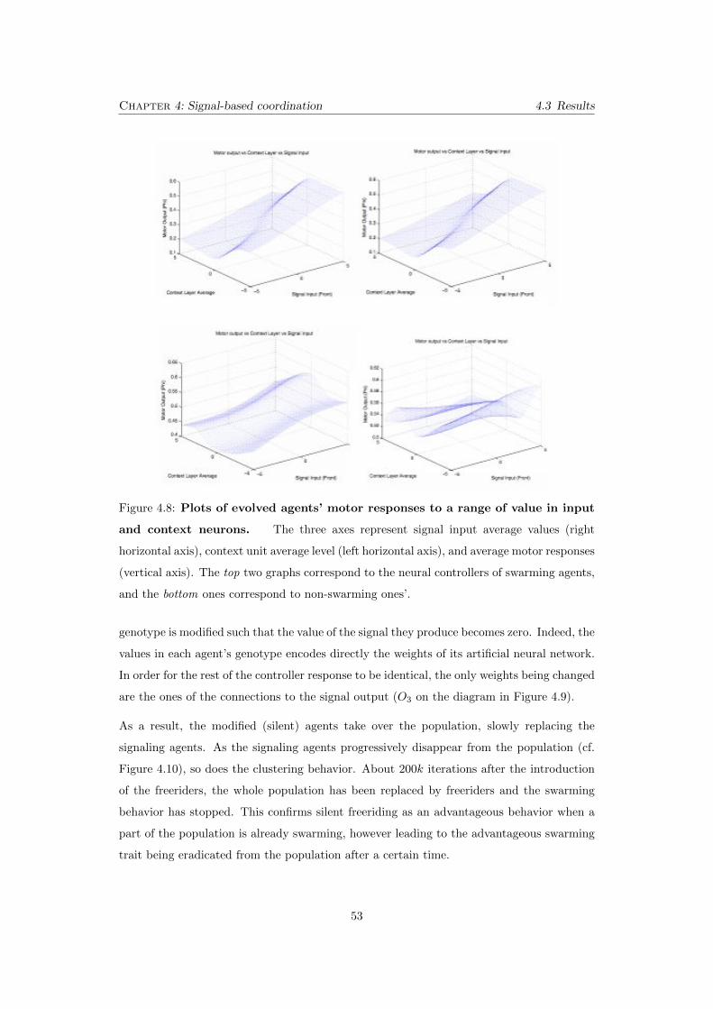
Chapter 4: Signal-based coordination 4.3 Results
Figure 4.8: Plots of evolved agents’ motor responses to a range of value in input
and context neurons. The three axes represent signal input average values (right
horizontal axis), context unit average level (left horizontal axis), and average motor responses
(vertical axis). The top two graphs correspond to the neural controllers of swarming agents,
and the bottom ones correspond to non-swarming ones’.
genotype is modified such that the value of the signal they produce becomes zero. Indeed, the
values in each agent’s genotype encodes directly the weights of its artificial neural network.
In order for the rest of the controller response to be identical, the only weights being changed
are the ones of the connections to the signal output (O3
on the diagram in Figure 4.9).
As a result, the modified (silent) agents take over the population, slowly replacing the
signaling agents. As the signaling agents progressively disappear from the population (cf.
Figure 4.10), so does the clustering behavior. About 200k iterations after the introduction
of the freeriders, the whole population has been replaced by freeriders and the swarming
behavior has stopped. This confirms silent freeriding as an advantageous behavior when a
part of the population is already swarming, however leading to the advantageous swarming
trait being eradicated from the population after a certain time.
53
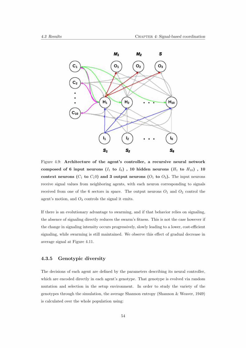
4.3 Results Chapter 4: Signal-based coordination
Figure 4.9: Architecture of the agent’s controller, a recursive neural network
composed of 6 input neurons (I1
to I6
) , 10 hidden neurons (H1
to H10
) , 10
context neurons (C1
to C1
0) and 3 output neurons (O1
to O3
). The input neurons
receive signal values from neighboring agents, with each neuron corresponding to signals
received from one of the 6 sectors in space. The output neurons O1
and O2
control the
agent’s motion, and O3
controls the signal it emits.
If there is an evolutionary advantage to swarming, and if that behavior relies on signaling,
the absence of signaling directly reduces the swarm’s fitness. This is not the case however if
the change in signaling intensity occurs progressively, slowly leading to a lower, cost-e�cient
signaling, while swarming is still maintained. We observe this e↵ect of gradual decrease in
average signal at Figure 4.11.
4.3.5 Genotypic diversity
The decisions of each agent are defined by the parameters describing its neural controller,
which are encoded directly in each agent’s genotype. That genotype is evolved via random
mutation and selection in the setup environment. In order to study the variety of the
genotypes through the simulation, the average Shannon entropy (Shannon & Weaver, 1949)
is calculated over the whole population using:
54
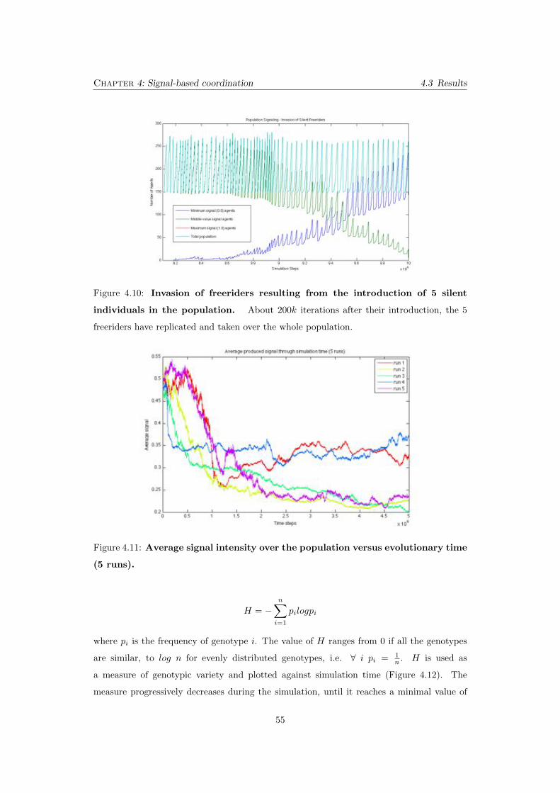
Chapter 4: Signal-based coordination 4.3 Results
Figure 4.10: Invasion of freeriders resulting from the introduction of 5 silent
individuals in the population. About 200k iterations after their introduction, the 5
freeriders have replicated and taken over the whole population.
Figure 4.11: Average signal intensity over the population versus evolutionary time
(5 runs).
H = �nX
i=1
pilogpi
where pi is the frequency of genotype i. The value of H ranges from 0 if all the genotypes
are similar, to log n for evenly distributed genotypes, i.e. 8 i pi = 1
n . H is used as
a measure of genotypic variety and plotted against simulation time (Figure 4.12). The
measure progressively decreases during the simulation, until it reaches a minimal value of
55
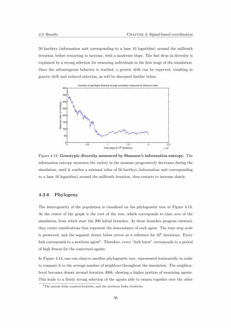
4.3 Results Chapter 4: Signal-based coordination
50 hartleys (information unit corresponding to a base 10 logarithm) around the millionth
iteration, before restarting to increase, with a moderate slope. The fast drop in diversity is
explained by a strong selection for swarming individuals in the first stage of the simulation.
Once the advantageous behavior is reached, a genetic drift can be expected, resulting in
genetic drift and reduced selection, as will be discussed further below.
0 0.5 1 1.5 2 2.5
x 106
0
50
100
150
200
250
300
350
400
Time steps (2 106 iterations)
Sh
an
no
n in
de
x (in
ha
rtle
ys)
Evolution of genotypic diversity through simulation measured by Shannon index
Figure 4.12: Genotypic diversity measured by Shannon’s information entropy. The
information entropy measures the variety in the measure progressively decreases during the
simulation, until it reaches a minimal value of 50 hartleys (information unit corresponding
to a base 10 logarithm) around the millionth iteration, then restarts to increase slowly.
4.3.6 Phylogeny
The heterogeneity of the population is visualized on the phylogenetic tree at Figure 4.13.
At the center of the graph is the root of the tree, which corresponds to time zero of the
simulation, from which start the 200 initial branches. As those branches progress outward,
they create ramifications that represent the descendance of each agent. The time step scale
is preserved, and the segment drawn below serves as a reference for 105 iterations. Every
fork corresponds to a newborn agent5. Therefore, every “fork burst” corresponds to a period
of high fitness for the concerned agents.
In Figure 4.14, one can observe another phylogenetic tree, represented horizontally in order
to compare it to the average number of neighbors throughout the simulation. The neighbor-
hood becomes denser around iteration 400k, showing a higher portion of swarming agents.
This leads to a firstly strong selection of the agents able to swarm together over the other
5The parent forks counterclockwise, and the newborn forks clockwise.
56
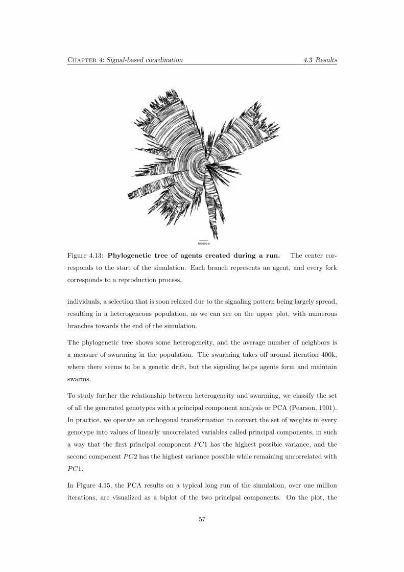
Chapter 4: Signal-based coordination 4.3 Results
Figure 4.13: Phylogenetic tree of agents created during a run. The center cor-
responds to the start of the simulation. Each branch represents an agent, and every fork
corresponds to a reproduction process.
individuals, a selection that is soon relaxed due to the signaling pattern being largely spread,
resulting in a heterogeneous population, as we can see on the upper plot, with numerous
branches towards the end of the simulation.
The phylogenetic tree shows some heterogeneity, and the average number of neighbors is
a measure of swarming in the population. The swarming takes o↵ around iteration 400k,
where there seems to be a genetic drift, but the signaling helps agents form and maintain
swarms.
To study further the relationship between heterogeneity and swarming, we classify the set
of all the generated genotypes with a principal component analysis or PCA (Pearson, 1901).
In practice, we operate an orthogonal transformation to convert the set of weights in every
genotype into values of linearly uncorrelated variables called principal components, in such
a way that the first principal component PC1 has the highest possible variance, and the
second component PC2 has the highest variance possible while remaining uncorrelated with
PC1.
In Figure 4.15, the PCA results on a typical long run of the simulation, over one million
iterations, are visualized as a biplot of the two principal components. On the plot, the
57
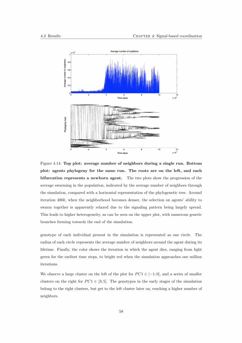
4.3 Results Chapter 4: Signal-based coordination
Figure 4.14: Top plot: average number of neighbors during a single run. Bottom
plot: agents phylogeny for the same run. The roots are on the left, and each
bifurcation represents a newborn agent. The two plots show the progression of the
average swarming in the population, indicated by the average number of neighbors through
the simulation, compared with a horizontal representation of the phylogenetic tree. Around
iteration 400k, when the neighborhood becomes denser, the selection on agents’ ability to
swarm together is apparently relaxed due to the signaling pattern being largely spread.
This leads to higher heterogeneity, as can be seen on the upper plot, with numerous genetic
branches forming towards the end of the simulation.
genotype of each individual present in the simulation is represented as one circle. The
radius of each circle represents the average number of neighbors around the agent during its
lifetime. Finally, the color shows the iteration in which the agent dies, ranging from light
green for the earliest time steps, to bright red when the simulation approaches one million
iterations.
We observe a large cluster on the left of the plot for PC1 2 [�1; 0], and a series of smaller
clusters on the right for PC1 2 [3; 5]. The genotypes in the early stages of the simulation
belong to the right clusters, but get to the left cluster later on, reaching a higher number of
neighbors.
58
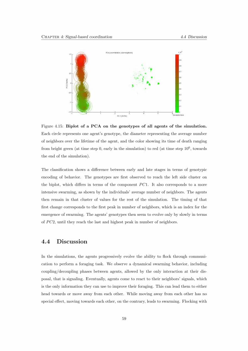
Chapter 4: Signal-based coordination 4.4 Discussion
Figure 4.15: Biplot of a PCA on the genotypes of all agents of the simulation.
Each circle represents one agent’s genotype, the diameter representing the average number
of neighbors over the lifetime of the agent, and the color showing its time of death ranging
from bright green (at time step 0, early in the simulation) to red (at time step 106, towards
the end of the simulation).
The classification shows a di↵erence between early and late stages in terms of genotypic
encoding of behavior. The genotypes are first observed to reach the left side cluster on
the biplot, which di↵ers in terms of the component PC1. It also corresponds to a more
intensive swarming, as shown by the individuals’ average number of neighbors. The agents
then remain in that cluster of values for the rest of the simulation. The timing of that
first change corresponds to the first peak in number of neighbors, which is an index for the
emergence of swarming. The agents’ genotypes then seem to evolve only by slowly in terms
of PC2, until they reach the last and highest peak in number of neighbors.
4.4 Discussion
In the simulations, the agents progressively evolve the ability to flock through communi-
cation to perform a foraging task. We observe a dynamical swarming behavior, including
coupling/decoupling phases between agents, allowed by the only interaction at their dis-
posal, that is signaling. Eventually, agents come to react to their neighbors’ signals, which
is the only information they can use to improve their foraging. This can lead them to either
head towards or move away from each other. While moving away from each other has no
special e↵ect, moving towards each other, on the contrary, leads to swarming. Flocking with
59
4.4 Discussion Chapter 4: Signal-based coordination
each other may lead agents to slow down their pace, which for some of them may keep them
closer to a food resource. This creates a beneficial feedback loop, since the fitness brought to
the agents will allow them to reproduce faster, and eventually multiply this type of behavior
within the total population.
In this scenario, agents do not need extremely complex learning to swarm and eventually get
more easily to the resource, but rather rely on dynamics emerging from their communication
system to create inertia and remain close to goal areas.
It should be noted that the simulated population has strong heterogeneity due to the asyn-
chronous reproduction schema, which can be visualized in the phylogenetic tree (Figure
4.13). Such heterogeneity may suppress swarming but the evolved signaling helps the popu-
lation to form and keep swarming. The simulations do not exhibit strong selection pressures
to adopt specific behavior apart from the use of the signaling. Without high homogeneity in
the population, the signaling alone allows for interaction dynamics su�cient to form swarms,
which proves in turn to be beneficial to get extra fitness as mentioned above.
The results suggest that by coordinating in clusters, the agents enter an evolutionary neutral
space, where little selection is applied to their genotypes. The formation of swarms acts as
a shield on the selection process, as a consequence allowing for the genotypes to drift. This
relaxation of selection can be compared to a niche construction, in which the system is ready
to adapt to further optimizations to the surrounding environment. This can be examined
in further research by the addition of a secondary task.
In the presented model, the population of genotypes progressively reach the part of the
search space that corresponds to swarming, as it helps agents achieve a higher fitness. The
behavioral transition between non-swarming and swarming happens relatively abruptly, and
can be caused by either the individual behavior improving enough or the population dy-
namical state satisfying certain conditions, or a combination of both. The latter one is
highlighted by the variable amount of time necessary before swarms can reform after the
positions have been randomized, thus illustrating the concept of collective memory in groups
of self-propelled individuals. Indeed, although one agent’s behavior is dictated by its geno-
type, the swarming also depends on the collective state of the neighborhood. Couzin et al.
(2002) brought to attention that even for identical individual behaviors, the previous history
of a group structure can change its dynamics. In the light of that fact, reaching the neutral
space relies on more than just the individual’s genetic heritage.
The phenomenon of freeriding, observed when artificially introducing silent individuals, is
60
Chapter 4: Signal-based coordination 4.4 Discussion
comparable to a tragedy of the commons (ToC) or an evolutionary suicide, in which an
evolved selfish behavior can harm the whole population’s survival [Haldane 1932, Hardin
1968]. This e↵ect, here provoked artificially, is however unlikely to happen in our setup, as
the decrease in produced signal intensity would progressively result in an ine�cient perfor-
mance, with a smooth decrease of fitness over the search space. The ToC has better chances
to arise in a setup with a larger map, in which parts of the population can be isolated for a
longer time, leading to di↵erent populations evolving separately, until they meet again and
confront their behaviors.
The results of this research can be compared to previous works in the literature. Ward et al.
(2001) and Olson et al. (2013) also show the emergence of swarming without explicit fit-
ness, though those are based on a predator-prey model. The type of swarming obtained with
simple pressures is usually similar to the one obtained in this study, that presents the advan-
tage of being based on a very simple system based on resource finding and signaling/sensing.
Among others, Blondel et al. (2005), Cucker & Huepe (2008) and Su et al. (2009) achieve
swarming behavior based on explicit exchange of information from leaders. Our simulation
improves on this kind of research in the sense that agents naturally switch leadership and
followership by exchanging information over a very limited channel of communication. Fi-
nally, our results also show the advantage of swarming for resource finding (it’s only through
swarming, enabled by signaling behavior, that agents are able to reach and remain around
the goal areas), comparable to the advantages of particle swarm optimizations (Kennedy
et al., 1995), here emerging in a model with a simplistic set of conditions.
In this work we have shown that swarming behavior can emerge from a communication
system in a resource gathering task. We implemented a three-dimensional agent-based model
with an asynchronous evolution through mutation and selection. The results show that
from decentralized leader-follower interactions, a population of agents can evolve collective
motion, in turn improving its fitness by reaching invisible target areas. Our results represent
an improvement on models using hard-coded rules to simulate swarming behavior, as they
are evolved from very simple conditions. The model does not rely on any explicit information
from leaders, nor does it impose any explicit leader-follower relationship beforehand, letting
simply the leader-follower dynamics emerge and self-organize. In spite of being theoretical,
the swarming model presented here o↵ers a simple, general approach to the emergence of
swarming behavior once approached via the boids’ rules.
In the perspective of this thesis, this first research led to the development of the most
61

4.4 Discussion Chapter 4: Signal-based coordination
minimalistic model of this thesis, that leads to the emergence of a communication system
helping the agents to coordinate together. This chapter constitutes the central piece in our
exploration of the evolution of coordination and communication, as it enables us to build up
on the same approach by complexifying the environment and its feedback on the population
of agents. In the next chapters, we will examine variations of this simple setup, to investigate
further the behavior and stability of coordination based on various types of exchanges of
information.
62
Chapter5Cooperative coordination in a dynamic
spatial Prisoner’s Dilemma
The evolution of cooperation is studied in game theory, and stretches have been made to
include spatial dimensions, as mentioned in Section 2.3. This problem is often tackled by
using simple models, such as considering interactions to be a game of Prisoner’s Dilemma
(PD)
We will now examine a variation of the model with a distinct fitness function, based this
time on the agents playing a spatial version of the Prisoner’s Dilemma. We study the impact
of the movement control on optimal strategies, and show that cooperators rapidly join into
static clusters, creating favorable niches for fast replications. It is also noted that, while
remaining inside those clusters, cooperators still keep moving faster than defectors. The
system dynamics are analyzed further to explain the stability of this behavior.
This chapter presents a model of simulated agents moving in a three-dimensional environ-
ment. Their movements are controlled by artificial networks, evolved through generations
of an asynchronous selection algorithm, at the term of which the agents become able to
produce cooperative, coordinated behavior.
We also introduce a variation of the model with a distinct fitness function based on the
agents’ performance on a spatial version of the Prisoner’s Dilemma. We investigate the
movement control in optimal strategies, and show that cooperators rapidly join into static
clusters, creating favorable niches for fast replications. It is also noted that, while remain-
ing inside those clusters, cooperators still keep moving faster than defectors. The system
dynamics are analyzed to explain the stability of this behavior.
63
5.1 Spatial Prisoner’s Dilemma Chapter 5: Cooperative coordination
5.1 Spatial Prisoner’s Dilemma
The problem of the evolution of cooperation has been of interest for a long time. This
problem is often tackled by using simple models, such as considering interactions to be a
game of Prisoner’s Dilemma (PD). Early results in game theory showed that cooperation
in the case of well-mixed population was not a given (Axelrod & Hamilton, 1981; Smith,
1982), yet it is a very common phenomenon in nature.
The PD is a classic two-player “game” in which players are given two options: cooperate (C)
or defect (D). The payo↵s are such that T > R > P > S, where T stands for Temptation (D
versus C), R for Reward (C versus C), P for punishment (D versus D) and S for Sucker’s
payo↵ (C versus D). It is also often admitted that 2R > T +S, meaning that cooperating is
overall better for the whole system, while defecting is better for the individual. In particular,
T > R and P > S means that it is always the best choice for an individual to defect, no
matter the strategy of its opponent. In a system where everyone can interact with everyone
else, without memory of past games or ways to distinguish opponents, defecting is obviously
the best strategy. However, it has been shown that spacial locality helps cooperators survive
and even thrive (Nowak & May, 1993).
This early work has triggered several lines of investigation, in particular attempts to add
movement. While results can be mixed in specific cases (Sicardi et al., 2009), it is widely
recognized that movement is helpful (Vainstein et al., 2007). Particular interest has been
given to random movement (Chen et al., 2011; Gelimson et al., 2013). In this case, though, we
argue that this movement acts as a way to restrict the neighborhood of specific individuals,
thus increasing locality. Di↵usion (Vainstein & Arenzon, 2014) is another example where
the environment is sparse, allowing agents to move to empty areas. Interesting dynamics
can also be obtained when the agents can actually choose on their own when and/or where
to move (Aktipis, 2004, 2011).
In this work , we investigate the impact of limited movement control on agents in a three
dimensional space. Agents are all moving at a common constant speed, but choose their
direction through the output of a neural network. We also add the possibility to communi-
cate, through the emission of signals. Such communication might be similar to greenbeards,
a phenomenon where an otherwise useless phenotype element is used to choose whether
to cooperate or not (see for instance Gardner & West (2010)). We argue, however, that
a slightly di↵erent mechanism is at work in our case. Indeed, since the signal is also an
64
Chapter 5: Cooperative coordination 5.2 Model
output of the neural network, agents can adapt their response to the environment. Signals
may be used both to detect where friendly agents are, or as a way to choose a strategy. In
this last case, cooperation can arise both from the fact that related agents will have similar
signaling (as in kin selection), or the adaptability of an external agent (mimicry). We show
that, when left to their own devices, cooperators will move more than defectors, even though
their cluster is static. They also tend to communicate much more than defectors, displaying
a complex dynamic to prevent defectors from taking over. We also show that speed matters,
as it impacts the radius of the clusters.
In the following, we describe the details of the model used in our experiments. Then,
we present the proportion of cooperators over time, and compare it to the static case (no
movement allowed). We also show other metrics, such as the average displacement over
time and the amount of received signal over time. We then analyse those results and give a
simple condition on the survival of a cluster before concluding.
5.2 Model
The model presented in this chapter builds up on the work described in detail in section 4.2.
However, given the number of tiny changes operated to adapt the model to the PD game, a
brief description is presented again here.
A population of agents move around in a three-dimensional space. Each one is playing
the Prisoner’s Dilemma game with its direct neighbors. The strategies are evolved via a
continuous genetic algorithm, that is agents with high level of fitness are allowed to replicate
with mutation whenever possible.
5.2.1 Environment
Agents are placed in a three-dimensional world with periodic boundary conditions. While
most previous work focuses on two-dimensional simulation, a third dimension gives the
system more freedom of movement, making it easier to choose not to play (i.e. move away).
The environment is a toroidal cube of size 600 (arbitrary unit), where each face connects
directly to the opposite one. The world is considered to be continuous, so that agents can
get arbitrarily close to each other (Figure 5.1), up to the precision of the simulation. Thus,
the dimensionality of the simulation comes down to the choice of the agent’s interaction
65
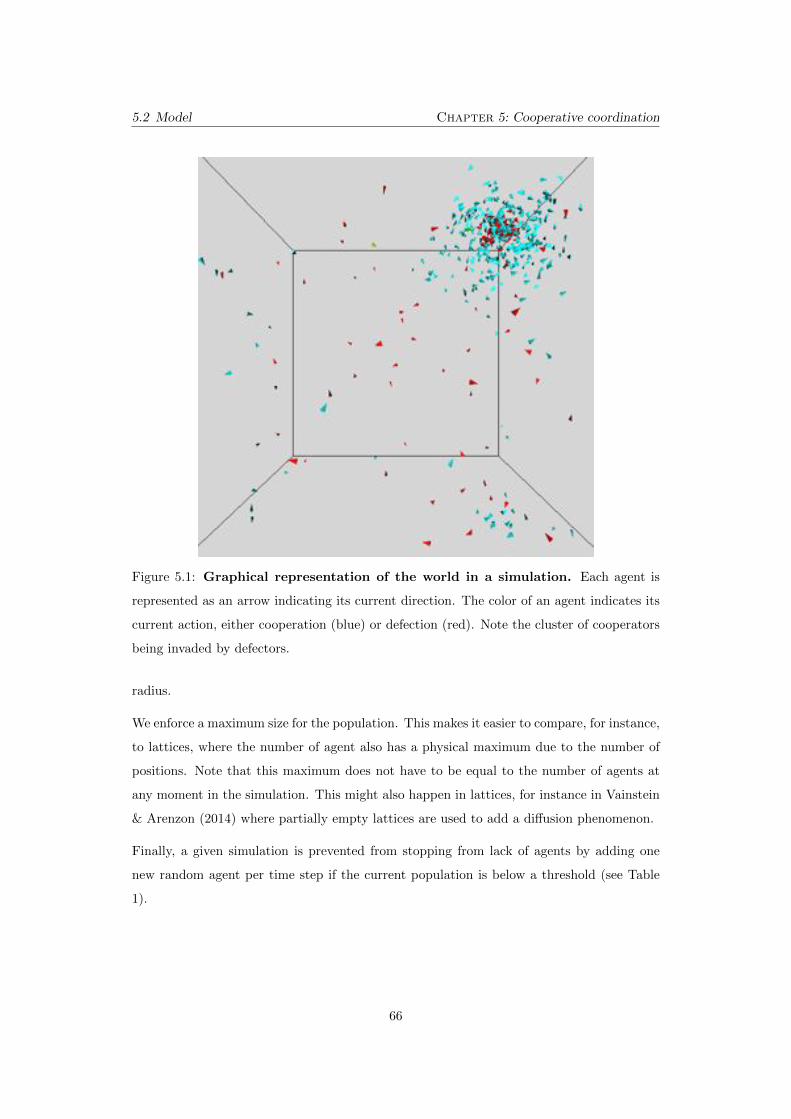
5.2 Model Chapter 5: Cooperative coordination
Figure 5.1: Graphical representation of the world in a simulation. Each agent is
represented as an arrow indicating its current direction. The color of an agent indicates its
current action, either cooperation (blue) or defection (red). Note the cluster of cooperators
being invaded by defectors.
radius.
We enforce a maximum size for the population. This makes it easier to compare, for instance,
to lattices, where the number of agent also has a physical maximum due to the number of
positions. Note that this maximum does not have to be equal to the number of agents at
any moment in the simulation. This might also happen in lattices, for instance in Vainstein
& Arenzon (2014) where partially empty lattices are used to add a di↵usion phenomenon.
Finally, a given simulation is prevented from stopping from lack of agents by adding one
new random agent per time step if the current population is below a threshold (see Table
1).
66
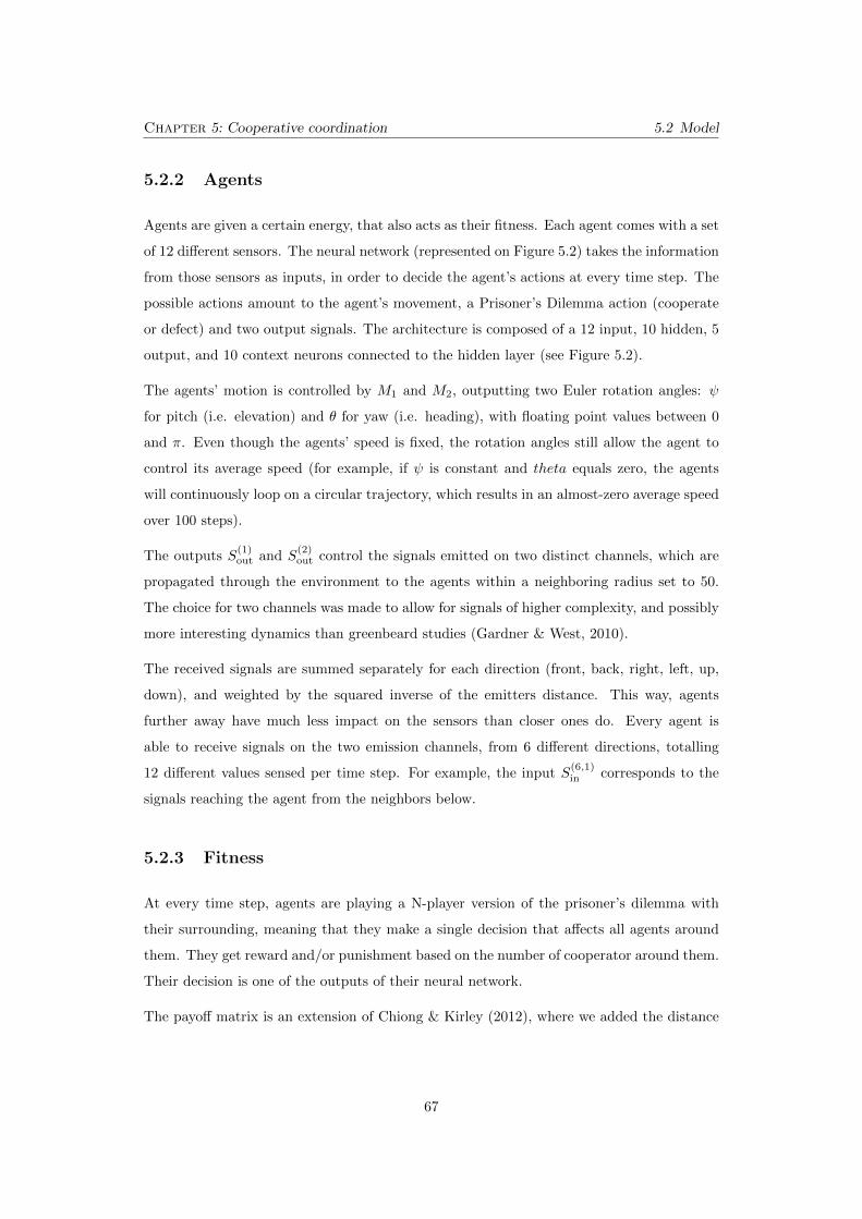
Chapter 5: Cooperative coordination 5.2 Model
5.2.2 Agents
Agents are given a certain energy, that also acts as their fitness. Each agent comes with a set
of 12 di↵erent sensors. The neural network (represented on Figure 5.2) takes the information
from those sensors as inputs, in order to decide the agent’s actions at every time step. The
possible actions amount to the agent’s movement, a Prisoner’s Dilemma action (cooperate
or defect) and two output signals. The architecture is composed of a 12 input, 10 hidden, 5
output, and 10 context neurons connected to the hidden layer (see Figure 5.2).
The agents’ motion is controlled by M1
and M2
, outputting two Euler rotation angles:
for pitch (i.e. elevation) and ✓ for yaw (i.e. heading), with floating point values between 0
and ⇡. Even though the agents’ speed is fixed, the rotation angles still allow the agent to
control its average speed (for example, if is constant and theta equals zero, the agents
will continuously loop on a circular trajectory, which results in an almost-zero average speed
over 100 steps).
The outputs S(1)
out
and S(2)
out
control the signals emitted on two distinct channels, which are
propagated through the environment to the agents within a neighboring radius set to 50.
The choice for two channels was made to allow for signals of higher complexity, and possibly
more interesting dynamics than greenbeard studies (Gardner & West, 2010).
The received signals are summed separately for each direction (front, back, right, left, up,
down), and weighted by the squared inverse of the emitters distance. This way, agents
further away have much less impact on the sensors than closer ones do. Every agent is
able to receive signals on the two emission channels, from 6 di↵erent directions, totalling
12 di↵erent values sensed per time step. For example, the input S(6,1)in
corresponds to the
signals reaching the agent from the neighbors below.
5.2.3 Fitness
At every time step, agents are playing a N-player version of the prisoner’s dilemma with
their surrounding, meaning that they make a single decision that a↵ects all agents around
them. They get reward and/or punishment based on the number of cooperator around them.
Their decision is one of the outputs of their neural network.
The payo↵ matrix is an extension of Chiong & Kirley (2012), where we added the distance
67
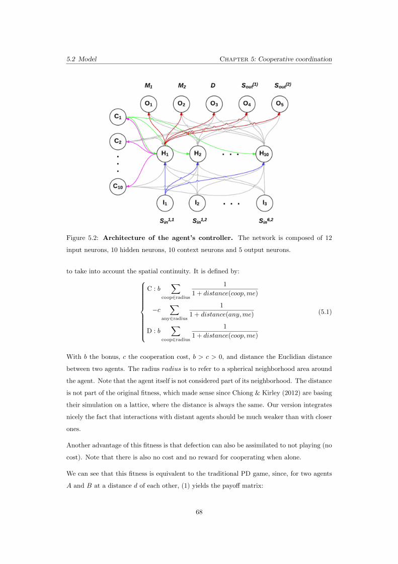
5.2 Model Chapter 5: Cooperative coordination
Figure 5.2: Architecture of the agent’s controller. The network is composed of 12
input neurons, 10 hidden neurons, 10 context neurons and 5 output neurons.
to take into account the spatial continuity. It is defined by:
8>>>>>>>>><
>>>>>>>>>:
C : bX
coop2radius
1
1 + distance(coop,me)
�cX
any2radius
1
1 + distance(any,me)
D : bX
coop2radius
1
1 + distance(coop,me)
(5.1)
With b the bonus, c the cooperation cost, b > c > 0, and distance the Euclidian distance
between two agents. The radius radius is to refer to a spherical neighborhood area around
the agent. Note that the agent itself is not considered part of its neighborhood. The distance
is not part of the original fitness, which made sense since Chiong & Kirley (2012) are basing
their simulation on a lattice, where the distance is always the same. Our version integrates
nicely the fact that interactions with distant agents should be much weaker than with closer
ones.
Another advantage of this fitness is that defection can also be assimilated to not playing (no
cost). Note that there is also no cost and no reward for cooperating when alone.
We can see that this fitness is equivalent to the traditional PD game, since, for two agents
A and B at a distance d of each other, (1) yields the payo↵ matrix:
68
Chapter 5: Cooperative coordination 5.3 Results
Initial energy 2
Maximum age 5000
Maximum energy 20
Maximum population size 500
Population threshold 100
Reproduction threshold 10
Reproduction cost 2
Reproduction radius 2
Survival cost per turn 2
Mutation rate (per gene) 0.05
Table 5.1: Parameters used for the simulation.
C D
C(b� c)
1 + d� c
1 + d
Db
1 + d0
It is clear that for the conditions b > c > 0, this matrix correspond to a PD.
Based on the outcome of the match, agents can choose a new direction, which is similar to
leaving the group in the walk away strategy (Aktipis, 2004), the main di↵erence being that,
in our case, it is also possible for groups to split. It is also similar in another aspect: there
is a cost to leaving a group, as a lone agent may need time to meet others.
5.2.4 Evolution/Parameters
The evolution is performed continuously over the population. Agents with negative or zero
energy are removed, while agents with energy above a threshold are forced to reproduce,
within the limits of one infant per time step. The reproduction cost is low enough, consid-
ering the threshold, to not put the life of the agent at risk. Table 5.1 indicates the various
parameters used for evolution.
5.3 Results
Results were obtained on a set of 10 runs, with additional sets used for control. In our setting,
all agents have a constant speed, but can choose in which direction they are heading. This
69
5.3 Results Chapter 5: Cooperative coordination
Figure 5.3: First quartile, average and third quartile of cooperation proportion
over 20 runs. Note that agents may choose at each time step which action (cooperation
or defection) they will perform, leading to high-frequency noise.
allows for pseudo-static behaviors by looping in circles.
While some characteristics, such as agents’ movement, were strongly run dependent, the
overall dynamics of the system was not. At the beginning of the run, the environment is
seeded with random agents. Since all weights in their neural network are set at random,
roughly half of the agents initially choose to cooperate while the other half choose to defect.
This leads to a fast extinction of cooperators (Figure 5.3, until approximately 50000 time
steps), until a group emerges strong enough to survive. The second phase follows, in which
cooperators are quickly increasing in number due to the autocatalytic nature of this strategy
(Figure 5.3).
A third step happens eventually, where defectors invade the cluster, followed either by the
survival of the cluster due to cooperators running away or a reboot of the cycle. In case
of survival, oscillations in the proportion of cooperators can be observed. However, this
phenomenon is averaged away over multiple runs, since period and phase of the oscillations
are not correlated from one experiment to the other. Figure 5.4 shows those oscillations in
a typical run. The frequency of those phenomenon is shown in Table 5.2.
As a control, we ran the simulation after removing the possibility for agents to move. In
this case, cooperators have much less to fear from defectors and quickly overtake the whole
population while defectors quickly exhaust their energy as well as the energy of their coop-
erative neighbors (Figure 5.5). Were a defector to appear near a cluster of cooperators, the
70
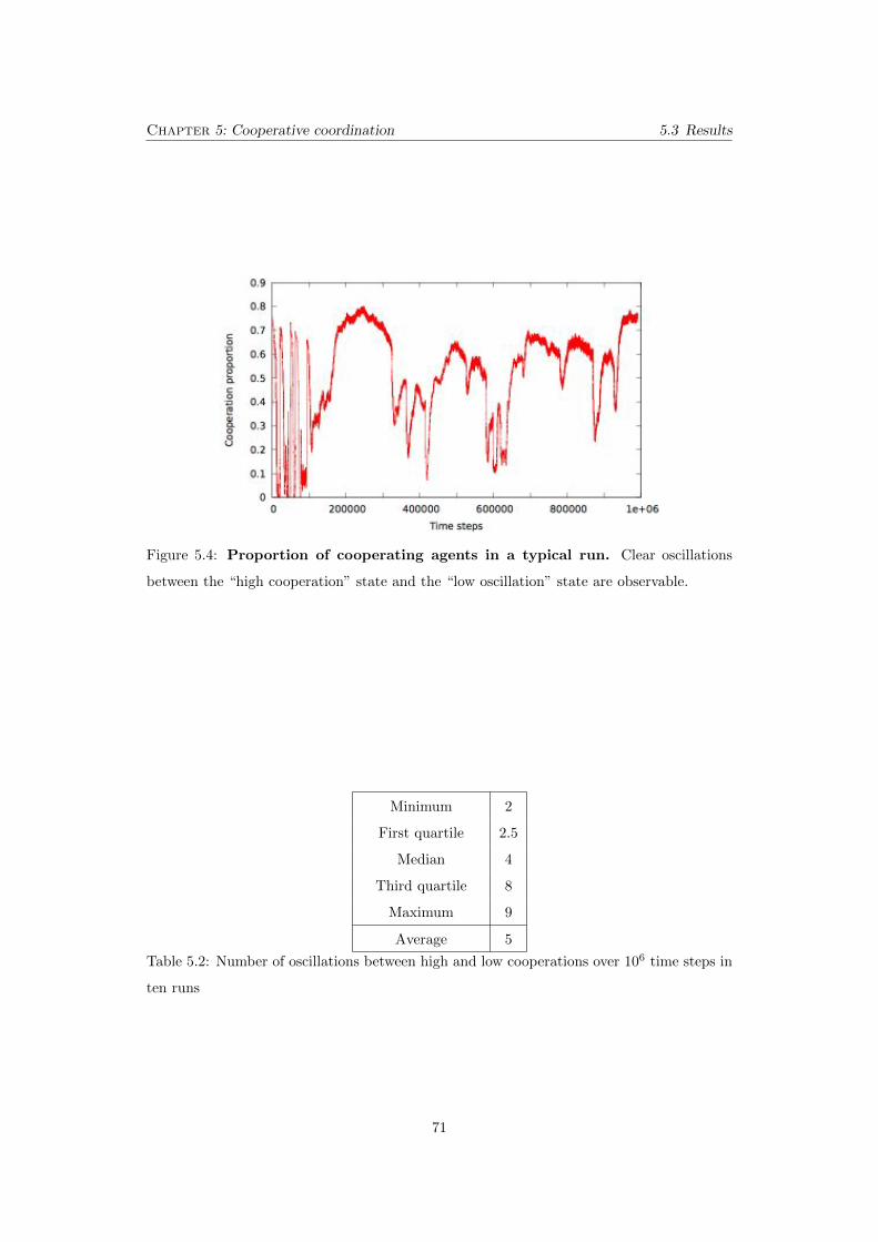
Chapter 5: Cooperative coordination 5.3 Results
Figure 5.4: Proportion of cooperating agents in a typical run. Clear oscillations
between the “high cooperation” state and the “low oscillation” state are observable.
Minimum 2
First quartile 2.5
Median 4
Third quartile 8
Maximum 9
Average 5
Table 5.2: Number of oscillations between high and low cooperations over 106 time steps in
ten runs
71
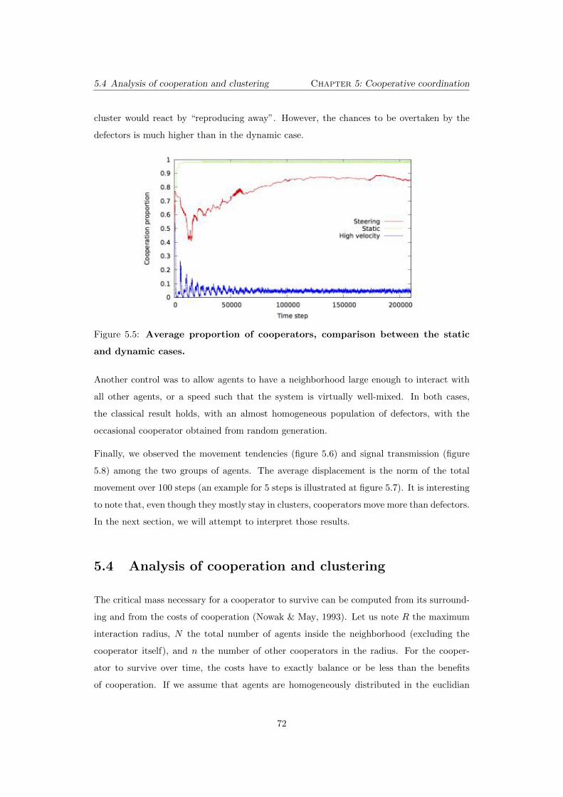
5.4 Analysis of cooperation and clustering Chapter 5: Cooperative coordination
cluster would react by “reproducing away”. However, the chances to be overtaken by the
defectors is much higher than in the dynamic case.
Figure 5.5: Average proportion of cooperators, comparison between the static
and dynamic cases.
Another control was to allow agents to have a neighborhood large enough to interact with
all other agents, or a speed such that the system is virtually well-mixed. In both cases,
the classical result holds, with an almost homogeneous population of defectors, with the
occasional cooperator obtained from random generation.
Finally, we observed the movement tendencies (figure 5.6) and signal transmission (figure
5.8) among the two groups of agents. The average displacement is the norm of the total
movement over 100 steps (an example for 5 steps is illustrated at figure 5.7). It is interesting
to note that, even though they mostly stay in clusters, cooperators move more than defectors.
In the next section, we will attempt to interpret those results.
5.4 Analysis of cooperation and clustering
The critical mass necessary for a cooperator to survive can be computed from its surround-
ing and from the costs of cooperation (Nowak & May, 1993). Let us note R the maximum
interaction radius, N the total number of agents inside the neighborhood (excluding the
cooperator itself), and n the number of other cooperators in the radius. For the cooper-
ator to survive over time, the costs have to exactly balance or be less than the benefits
of cooperation. If we assume that agents are homogeneously distributed in the euclidian
72
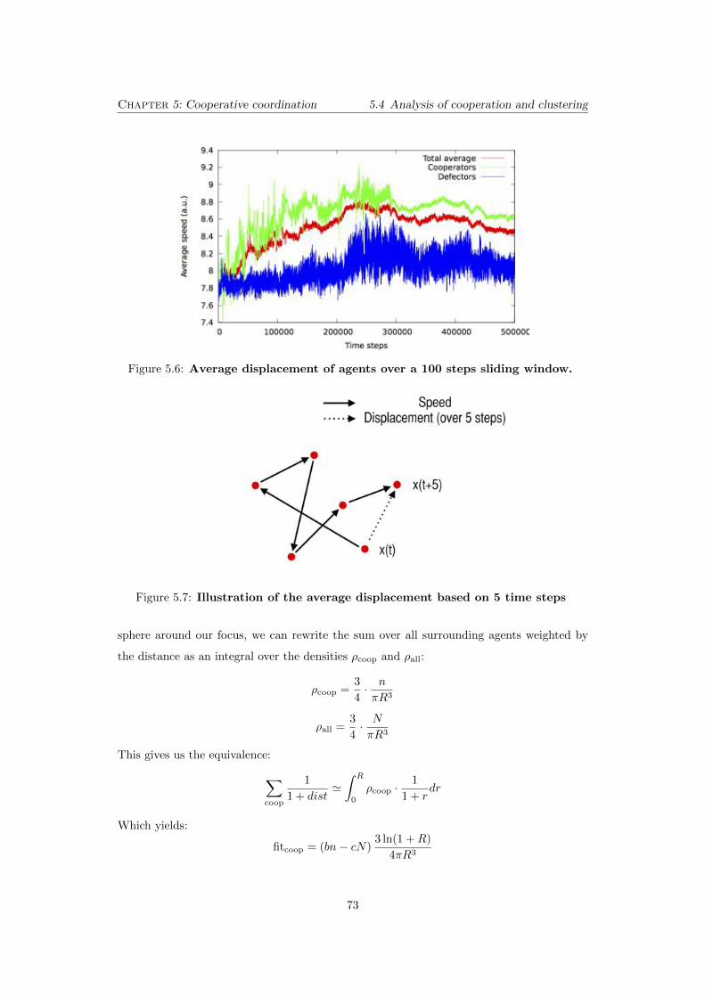
Chapter 5: Cooperative coordination 5.4 Analysis of cooperation and clustering
Figure 5.6: Average displacement of agents over a 100 steps sliding window.
Figure 5.7: Illustration of the average displacement based on 5 time steps
sphere around our focus, we can rewrite the sum over all surrounding agents weighted by
the distance as an integral over the densities ⇢coop
and ⇢all
:
⇢coop
=3
4· n
⇡R3
⇢all
=3
4· N
⇡R3
This gives us the equivalence:
X
coop
1
1 + dist'
Z R
0
⇢coop
· 1
1 + rdr
Which yields:
fitcoop
= (bn� cN)3 ln(1 + R)
4⇡R3
73
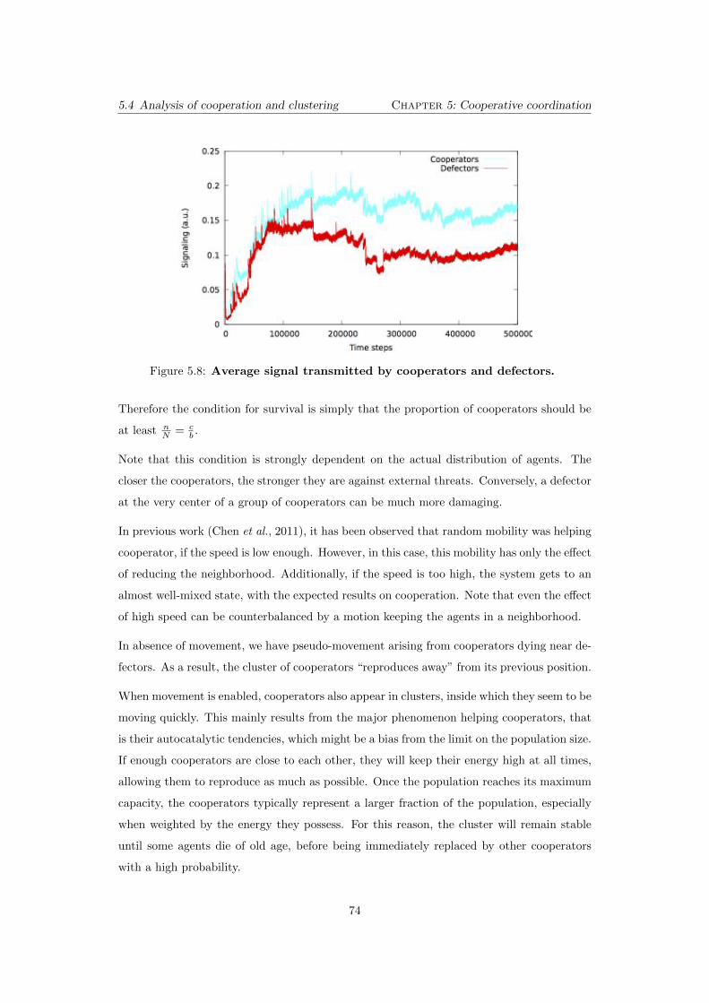
5.4 Analysis of cooperation and clustering Chapter 5: Cooperative coordination
Figure 5.8: Average signal transmitted by cooperators and defectors.
Therefore the condition for survival is simply that the proportion of cooperators should be
at least nN = c
b .
Note that this condition is strongly dependent on the actual distribution of agents. The
closer the cooperators, the stronger they are against external threats. Conversely, a defector
at the very center of a group of cooperators can be much more damaging.
In previous work (Chen et al., 2011), it has been observed that random mobility was helping
cooperator, if the speed is low enough. However, in this case, this mobility has only the e↵ect
of reducing the neighborhood. Additionally, if the speed is too high, the system gets to an
almost well-mixed state, with the expected results on cooperation. Note that even the e↵ect
of high speed can be counterbalanced by a motion keeping the agents in a neighborhood.
In absence of movement, we have pseudo-movement arising from cooperators dying near de-
fectors. As a result, the cluster of cooperators “reproduces away” from its previous position.
When movement is enabled, cooperators also appear in clusters, inside which they seem to be
moving quickly. This mainly results from the major phenomenon helping cooperators, that
is their autocatalytic tendencies, which might be a bias from the limit on the population size.
If enough cooperators are close to each other, they will keep their energy high at all times,
allowing them to reproduce as much as possible. Once the population reaches its maximum
capacity, the cooperators typically represent a larger fraction of the population, especially
when weighted by the energy they possess. For this reason, the cluster will remain stable
until some agents die of old age, before being immediately replaced by other cooperators
with a high probability.
74
Chapter 5: Cooperative coordination 5.5 Discussion
Also, this strategy might allow them to avoid spending too much time close to defectors,
while remaining constantly in the neighborhood of fellow cooperators.
The clustering is strongly dependent on signaling among the cooperating agents, hinted
by the di↵erence in signal emission between cooperators and defectors. Additionally, we
performed two batches of five control runs with respectively signal on or o↵ the whole time.
In the “o↵” case, no cluster can form, yielding a near-uniform population of defectors. The
“on” case still shows qualitatively the emergence of clusters, but are much more di↵use as
signaling is now ambiguous.
5.5 Discussion
In this work, we introduced a three-dimensional model of agents playing the Prisoner’s
Dilemma. A first result is that cooperators, when they are present, quickly evolve to form
clusters as they represent a favorable pattern. The clustering behavior can be interpreted
as a degenerated version of the simulations presented in Chapter 4, since the cooperating
agents present the same capacities of information exchange as that model. The possibility
of this degeneracy is mentioned in Section 4.2.4.
While the clustering itself can be expected, it is interesting to observe that their overall
movement rate is still higher than defectors. This is even more surprising considering that
those clusters do not seem to move fast. Instead, analysis shows that cooperators are moving
quickly inside the cluster, which may be a way to adapt to an aggressive environment.
In addition, comparison with the static case showed that movement made the apparition
of cooperators harder, but more stable in the long run. Since it is harder for defectors to
overtake a cluster of cooperators, our systems often show a soft bistability, meaning that
they will eventually switch from one state to the other. It is even possible to observe a
sort of symbiosis, where cooperators are generating more energy than necessary, which is in
turn used by peripheral defectors. In this case, replacement rates allow cooperators to stay
ahead, keeping this small ecosystem stable.
This cohesion among cooperators seems to be enhanced by signaling, even though signals
might attract defectors. Additional investigation on the transfer entropy, for instance, could
be a promising next step.
Finally, another original contribution of this chapter resides in the choice of actions, which is
75
5.5 Discussion Chapter 5: Cooperative coordination
generated by the neural networks without consideration of the past actions. The interesting
point is the creation of a memory e↵ect, that usually requires to be encoded in each agent,
here emerging from the agents’ movements in space.
Recently, the Prisoner’s Dilemma game has become a paradigmatic model, used as a tool
in evolutionary biology to study the outcomes depending on the costs characterizing an
ecosystem. In this chapter, we have focused on a model with a fitness based on the results
of such game, and showed the emergence of spatial coordination based on a the exchange
of signals between agents. Like in Chapter 4, the signals remained very basic, and the
environment was fixed in time. In the next chapters, we will explore di↵erent types of com-
munication and variable resource environments, to test further the stability of the emergence
of communication and its impact on the evolution of group coordination.
76
Chapter6Synchronization in variable resource envi-
ronments
In behavioral ecology, populations change through the course of evolution, with each in-
dividual adapting to its environment. The individual’s adaptative behavior determines its
survival and reproductive success. The presence of other individuals a↵ects the environment
itself, causing all individuals to end up entangled in an interdependent interaction network.
Over successive generations, the organisms must adapt to their surrounding conditions in
order to develop their ecological niche. As structural changes occur in the external environ-
ment, the organisms’ niche has to evolve accordingly, building on prior knowledge acquired
by the population. In turn, this has the power to increase the survival and reproductive
success of the species.
In this chapter, we focus on adaptive behavior in the context of variable environments,
specifically with periodic fluctuations of resource availability. This naturally follows up on
Chapter 4, where coordinated behavior has been studied in stable ecological conditions.
When the environment is altered, the individuals can adapt to the new conditions either by
reacting to cues they are able to detect in the environment or by observing the behavior
of other individuals around them. In the following, we present three di↵erent simulations1
demonstrating the emergence of such adaptations, each based on di↵erent types of direct
or indirect information provided to the agents, and discuss the conditions giving rise to the
phenomenon.
In a first experiment, we use a model with dual seasonal change of food distribution in a
unidimensional space. The food resource is made plentiful in artificial summers, whereas
1As mentioned in the introduction of this thesis, the works presented in this chapter have preceded the
ones utilized in Chapters 4 and 5. They nevertheless belong here, as part of a study on adaptiveness in
environments with fluctuating resources.
77
6.1 Signaling in dynamic environments Chapter 6: Synchronization
it almost disappears in winters. In the simulation, the agents are observed to adapt by
slowing down their motion in winter to save energy, to wake up once the food distribution
becomes favorable again. This is realized not only by detecting the food scarcity but more
interestingly by reacting to the other agents’ signaling. The emergence of this coopera-
tive signaling behavior demonstrates a basic set of conditions leading to the emergence of
adaptive coordination.
In a second setup, we study the impact of seasons on agents’ coordination in a bidimensional
space. The food resource location switches between two di↵erent areas according to the
season, resulting in agents migrating from one to another. In order to find out the right
time to move, the agents rely again on other individuals’ signals. This study not only focuses
on the cooperative emergence of signaling, but also addresses the debate on the biological
component associated with the learning process in ecological adaptive behavior.
Finally, we present a third experiment with the direct communication channel this time
removed, the agents are only allowed to interact through resource consumption. Once again,
we look at the evolved foraging behavior through generations, to see how the information
is used by lineages of agents to take evolutionary advantageous paths. As a result of the
seasonal change, we observe the emergence of a resource caching behavior, depending on
agent size, also known as hoarding.
6.1 Signaling in dynamic environments
Many behaviors found in nature are tightly related to the abundance of resources in the
environment. In case of changes in the availability of those resources, the living organisms
need to adapt their strategies to survive. In such unpredictable environments, signaling has
been proposed as an adaptive behavior meant to filter out the reliable information (Levins,
1968; Johnstone, 1997; Torney et al., 2011).
In the field of artificial life, computational agent-based modelling is a popular synthetic ap-
proach. Such models attempt to replicate the evolutionary conditions responsible for group
behavior adaptation in response to the learning of symbolic or complex syntactical structures
(Parisi, 1997; Cangelosi, 2001). Communication plays a key role in social species, facilitating
crucial information transfer in a group and increasing its survival chances (Maynard-Smith
& Szathmary, 1997).
78
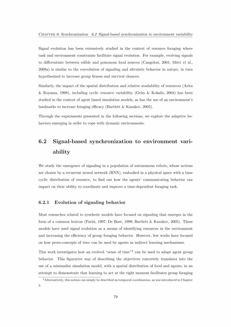
Chapter 6: Synchronization 6.2 Signal-based synchronization to environment variability
Signal evolution has been extensively studied in the context of resource foraging where
task and environment constraints facilitate signal evolution. For example, evolving signals
to di↵erentiate between edible and poisonous food sources (Cangelosi, 2001; Mitri et al.,
2009a) is similar to the coevolution of signaling and altruistic behavior in nature, in turn
hypothesized to increase group fitness and survival chances.
Similarly, the impact of the spatial distribution and relative availability of resources (Arita
& Koyama, 1998), including cyclic resource variability (Grim & Kokalis, 2004) has been
studied in the context of agent based simulation models, as has the use of an environment’s
landmarks to increase foraging e�cacy (Bartlett & Kazakov, 2005).
Through the experiments presented in the following sections, we explore the adaptive be-
haviors emerging in order to cope with dynamic environments.
6.2 Signal-based synchronization to environment vari-
ability
We study the emergence of signaling in a population of autonomous robots, whose actions
are chosen by a recurrent neural network (RNN), embodied in a physical space with a time
cyclic distribution of resource, to find out how the agents’ communicating behavior can
impact on their ability to coordinate and improve a time-dependent foraging task.
6.2.1 Evolution of signaling behavior
Most researches related to synthetic models have focused on signaling that emerges in the
form of a common lexicon (Parisi, 1997; De Boer, 1999; Bartlett & Kazakov, 2005). These
models have used signal evolution as a means of identifying resources in the environment
and increasing the e�ciency of group foraging behavior. However, few works have focused
on how proto-concepts of time can be used by agents as indirect learning mechanisms.
This work investigates how an evolved “sense of time”2 can be used to adapt agent group
behavior. This figurative way of describing the objectives concretely translates into the
use of a minimalist simulation model, with a spatial distribution of food and agents, in an
attempt to demonstrate that learning to act at the right moment facilitates group foraging
2Alternatively, this notion can simply be described as temporal coordination, as was introduced in Chapter
2.
79
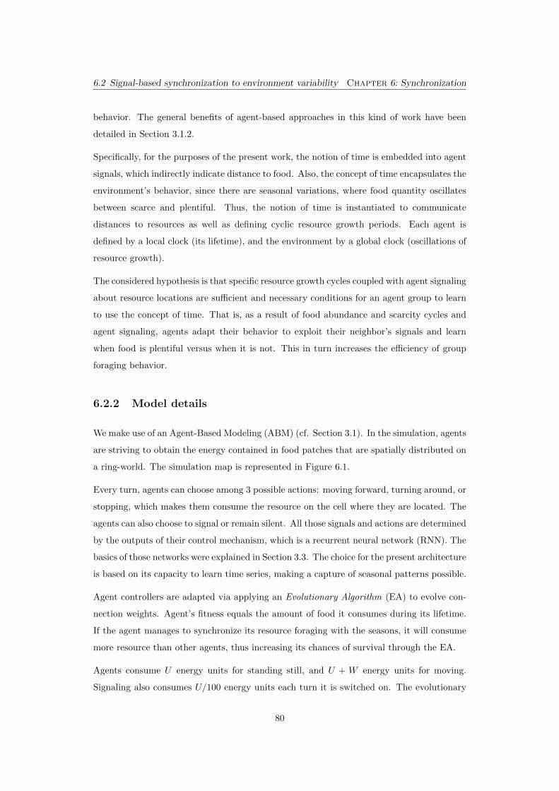
6.2 Signal-based synchronization to environment variability Chapter 6: Synchronization
behavior. The general benefits of agent-based approaches in this kind of work have been
detailed in Section 3.1.2.
Specifically, for the purposes of the present work, the notion of time is embedded into agent
signals, which indirectly indicate distance to food. Also, the concept of time encapsulates the
environment’s behavior, since there are seasonal variations, where food quantity oscillates
between scarce and plentiful. Thus, the notion of time is instantiated to communicate
distances to resources as well as defining cyclic resource growth periods. Each agent is
defined by a local clock (its lifetime), and the environment by a global clock (oscillations of
resource growth).
The considered hypothesis is that specific resource growth cycles coupled with agent signaling
about resource locations are su�cient and necessary conditions for an agent group to learn
to use the concept of time. That is, as a result of food abundance and scarcity cycles and
agent signaling, agents adapt their behavior to exploit their neighbor’s signals and learn
when food is plentiful versus when it is not. This in turn increases the e�ciency of group
foraging behavior.
6.2.2 Model details
We make use of an Agent-Based Modeling (ABM) (cf. Section 3.1). In the simulation, agents
are striving to obtain the energy contained in food patches that are spatially distributed on
a ring-world. The simulation map is represented in Figure 6.1.
Every turn, agents can choose among 3 possible actions: moving forward, turning around, or
stopping, which makes them consume the resource on the cell where they are located. The
agents can also choose to signal or remain silent. All those signals and actions are determined
by the outputs of their control mechanism, which is a recurrent neural network (RNN). The
basics of those networks were explained in Section 3.3. The choice for the present architecture
is based on its capacity to learn time series, making a capture of seasonal patterns possible.
Agent controllers are adapted via applying an Evolutionary Algorithm (EA) to evolve con-
nection weights. Agent’s fitness equals the amount of food it consumes during its lifetime.
If the agent manages to synchronize its resource foraging with the seasons, it will consume
more resource than other agents, thus increasing its chances of survival through the EA.
Agents consume U energy units for standing still, and U + W energy units for moving.
Signaling also consumes U/100 energy units each turn it is switched on. The evolutionary
80
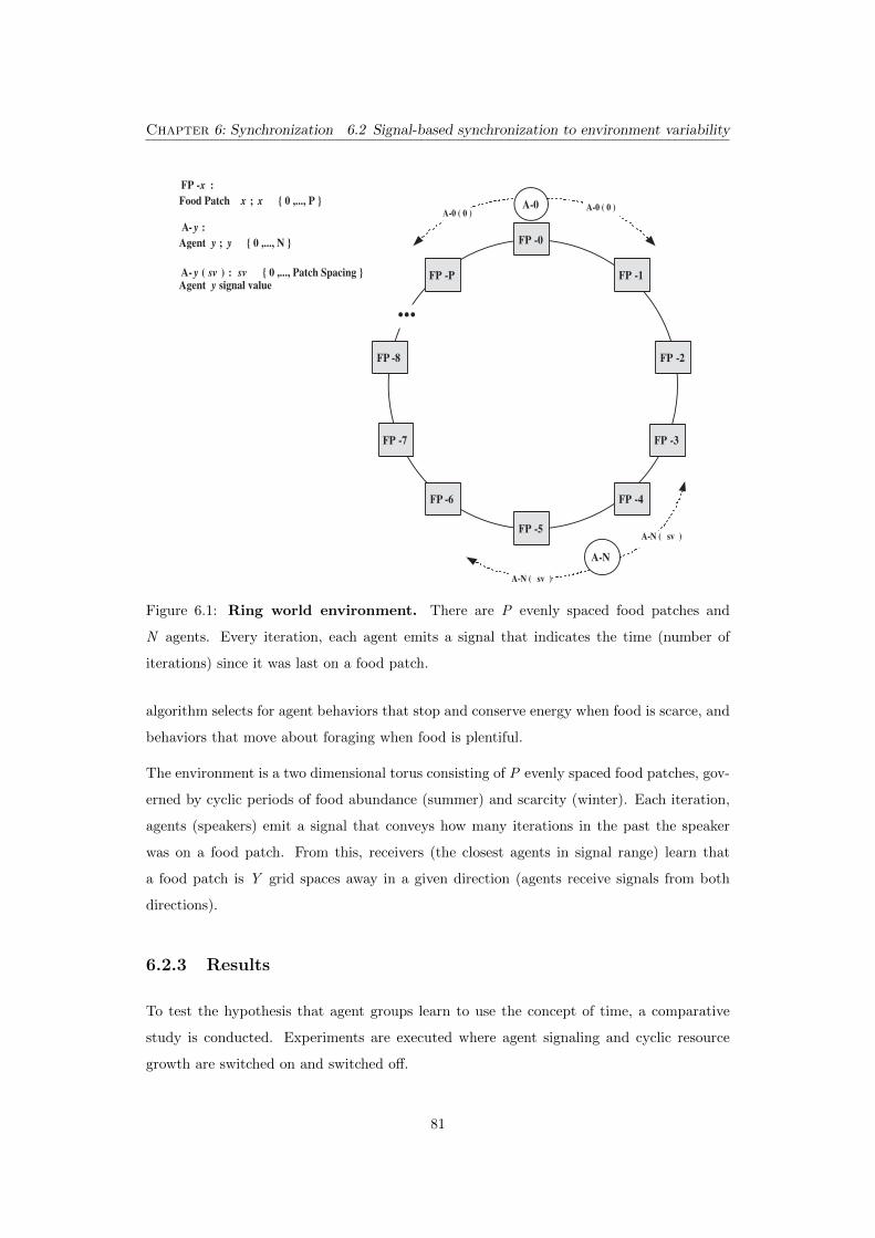
Chapter 6: Synchronization 6.2 Signal-based synchronization to environment variability
FP�-x� :�
Food Patch� x�;� x��� { 0 ,..., P }�
A�-�y�:�
Agent� y� ;� y��� { 0 ,..., N }�
A�-�y�(�sv� )� :� sv� �� { 0 ,..., Patch Spacing }�Agent� y� signal value�
FP�-0�
A-0�
FP�-5�
FP�-1�
FP�-4�
FP�-2�
FP�-P�
FP�-6�
FP�-8�
FP�-7� FP�-3�
A-N�
A-0 ( 0 )�A-0 ( 0 )�
A-N (� sv� )�
A-N (� sv� )�
...�
Figure 6.1: Ring world environment. There are P evenly spaced food patches and
N agents. Every iteration, each agent emits a signal that indicates the time (number of
iterations) since it was last on a food patch.
algorithm selects for agent behaviors that stop and conserve energy when food is scarce, and
behaviors that move about foraging when food is plentiful.
The environment is a two dimensional torus consisting of P evenly spaced food patches, gov-
erned by cyclic periods of food abundance (summer) and scarcity (winter). Each iteration,
agents (speakers) emit a signal that conveys how many iterations in the past the speaker
was on a food patch. From this, receivers (the closest agents in signal range) learn that
a food patch is Y grid spaces away in a given direction (agents receive signals from both
directions).
6.2.3 Results
To test the hypothesis that agent groups learn to use the concept of time, a comparative
study is conducted. Experiments are executed where agent signaling and cyclic resource
growth are switched on and switched o↵.
81
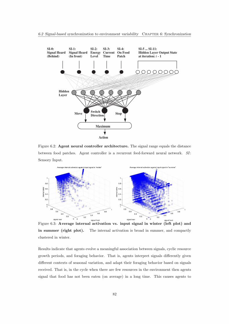
6.2 Signal-based synchronization to environment variability Chapter 6: Synchronization
SI-0:�Signal Heard�(Behind)�
MM�Maximum�
Action�
Hidden�Layer�
SI-1:�Signal Heard�(In front)�
SI-2:�Energy�Level�
SI-5 ... SI-11:�Hidden Layer Output State�at iteration:�t� - 1�
Stop�Move�Switch�Direction�
SI-3:�Current�Time�
SI-4:�On Food�Patch�
Figure 6.2: Agent neural controller architecture. The signal range equals the distance
between food patches. Agent controller is a recurrent feed-forward neural network. SI :
Sensory Input.
Figure 6.3: Average internal activation vs. input signal in winter (left plot) and
in summer (right plot). The internal activation is broad in summer, and compactly
clustered in winter.
Results indicate that agents evolve a meaningful association between signals, cyclic resource
growth periods, and foraging behavior. That is, agents interpret signals di↵erently given
di↵erent contexts of seasonal variation, and adapt their foraging behavior based on signals
received. That is, in the cycle when there are few resources in the environment then agents
signal that food has not been eaten (on average) in a long time. This causes agents to
82
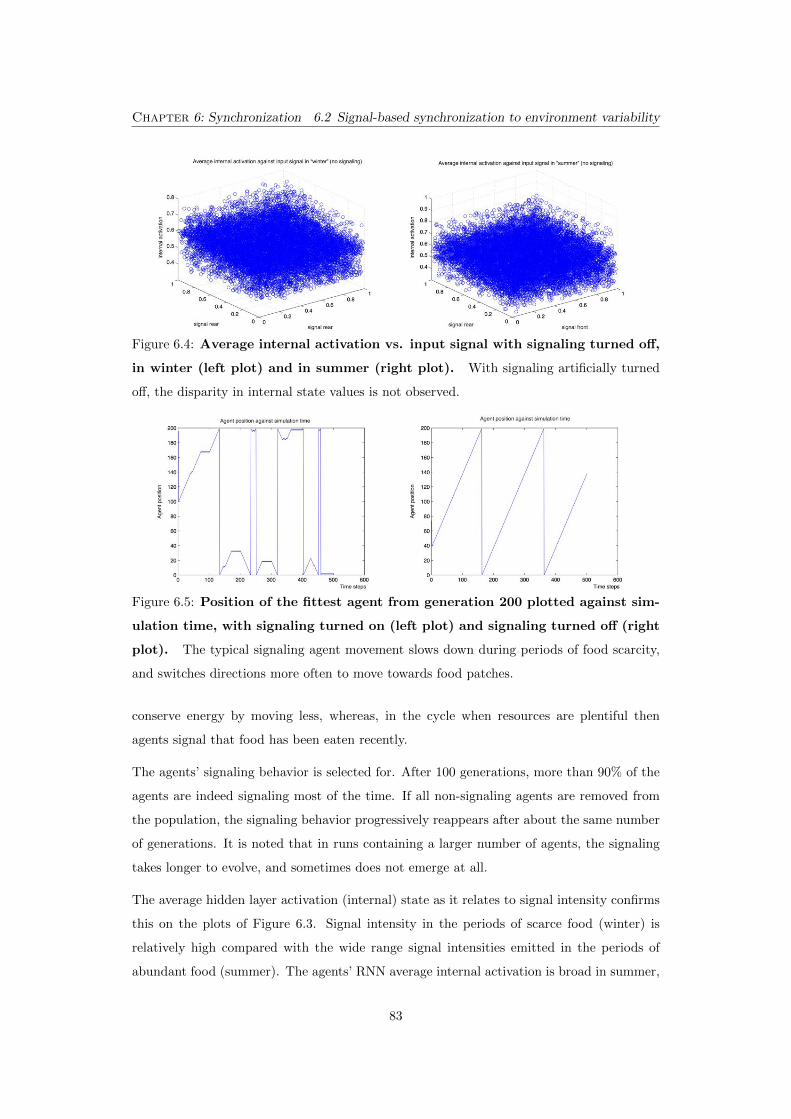
Chapter 6: Synchronization 6.2 Signal-based synchronization to environment variability
Figure 6.4: Average internal activation vs. input signal with signaling turned o↵,
in winter (left plot) and in summer (right plot). With signaling artificially turned
o↵, the disparity in internal state values is not observed.
Figure 6.5: Position of the fittest agent from generation 200 plotted against sim-
ulation time, with signaling turned on (left plot) and signaling turned o↵ (right
plot). The typical signaling agent movement slows down during periods of food scarcity,
and switches directions more often to move towards food patches.
conserve energy by moving less, whereas, in the cycle when resources are plentiful then
agents signal that food has been eaten recently.
The agents’ signaling behavior is selected for. After 100 generations, more than 90% of the
agents are indeed signaling most of the time. If all non-signaling agents are removed from
the population, the signaling behavior progressively reappears after about the same number
of generations. It is noted that in runs containing a larger number of agents, the signaling
takes longer to evolve, and sometimes does not emerge at all.
The average hidden layer activation (internal) state as it relates to signal intensity confirms
this on the plots of Figure 6.3. Signal intensity in the periods of scarce food (winter) is
relatively high compared with the wide range signal intensities emitted in the periods of
abundant food (summer). The agents’ RNN average internal activation is broad in summer,
83
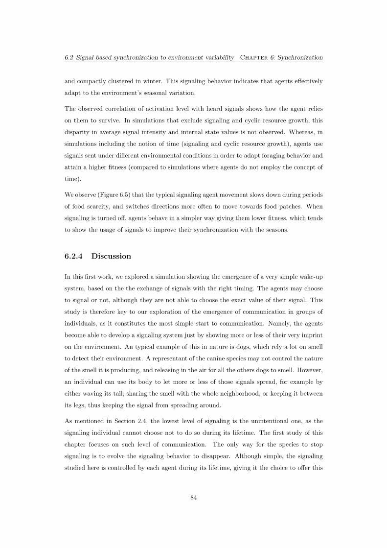
6.2 Signal-based synchronization to environment variability Chapter 6: Synchronization
and compactly clustered in winter. This signaling behavior indicates that agents e↵ectively
adapt to the environment’s seasonal variation.
The observed correlation of activation level with heard signals shows how the agent relies
on them to survive. In simulations that exclude signaling and cyclic resource growth, this
disparity in average signal intensity and internal state values is not observed. Whereas, in
simulations including the notion of time (signaling and cyclic resource growth), agents use
signals sent under di↵erent environmental conditions in order to adapt foraging behavior and
attain a higher fitness (compared to simulations where agents do not employ the concept of
time).
We observe (Figure 6.5) that the typical signaling agent movement slows down during periods
of food scarcity, and switches directions more often to move towards food patches. When
signaling is turned o↵, agents behave in a simpler way giving them lower fitness, which tends
to show the usage of signals to improve their synchronization with the seasons.
6.2.4 Discussion
In this first work, we explored a simulation showing the emergence of a very simple wake-up
system, based on the the exchange of signals with the right timing. The agents may choose
to signal or not, although they are not able to choose the exact value of their signal. This
study is therefore key to our exploration of the emergence of communication in groups of
individuals, as it constitutes the most simple start to communication. Namely, the agents
become able to develop a signaling system just by showing more or less of their very imprint
on the environment. An typical example of this in nature is dogs, which rely a lot on smell
to detect their environment. A representant of the canine species may not control the nature
of the smell it is producing, and releasing in the air for all the others dogs to smell. However,
an individual can use its body to let more or less of those signals spread, for example by
either waving its tail, sharing the smell with the whole neighborhood, or keeping it between
its legs, thus keeping the signal from spreading around.
As mentioned in Section 2.4, the lowest level of signaling is the unintentional one, as the
signaling individual cannot choose not to do so during its lifetime. The first study of this
chapter focuses on such level of communication. The only way for the species to stop
signaling is to evolve the signaling behavior to disappear. Although simple, the signaling
studied here is controlled by each agent during its lifetime, giving it the choice to o↵er this
84
Chapter 6: Synchronization 6.3 Mimicry and seasonal migratory synchronization
information to the other individuals or not.
In our simulations, based on their sharing of signals, the agents reach a coordinated state, in
which they adapt to each other’s signal they perceive to slow down or speed up their motion
based on the food distribution.
From the game theory view, the agents can be considered to take advantage of their neigh-
bors, given that the signal is there to be exploited. However the agents are free to turn
o↵ their signaling, allowing them to save their own energy, but eliminating the possibility
for their pairs to make use of the information. The choice to signal, which takes place in
the simulations, can be attributed to an altruist behavior. The emergence of cooperation is
linked to the associated costs (Axelrod & Hamilton, 1981), and a higher cost to signaling
would most naturally change the chances of cooperation ever coming about.
The results are compatible with the principle of kin selection (Smith, 1964; Williams, 1966;
Wilson, 1975), because a higher degree of relatedness – which happens in smaller populations
– can lead to higher levels of cooperation by a founder e↵ect (cf. Section 2.3). This is coherent
with larger populations having a harder time to evolve the signaling behavior. It can be
confirmed either by tuning the size of the population, or by isolating part of the population,
o↵ering a simple ABM-approach display of the role of bottlenecks and founder e↵ects in the
emergence of cooperation.
This first study in the present chapter showed that the synchronization based on very simple,
chosen but non-controlled signals allowed agents to improve their foraging behavior in a
resource variable environment. Next, we will look at variants of the model, starting with a
model introducing for a choice of signals for agents with their neighbors, along with an easy
way to imitate them.
6.3 Mimicry and seasonal migratory synchronization
In this second setup, agent-based modeling is used to investigate the adaptive coordination
resulting from a dynamic fitness landscape in two dimensions. The study is applied to
migratory behavior, which can be either genetically or culturally determined. Our model
aims to investigate the evolutionary and cultural conditions that give rise to migratory
behaviors and more generally adaptive foraging in dynamic fitness environments.
In cultural behavioral transmission, ontogenetic transfer occurs between agents during their
85
6.3 Mimicry and seasonal migratory synchronization Chapter 6: Synchronization
lifetime. Alternatively, migratory behavior is phylogenetically transmitted through succes-
sive generations. A minimalist simulation model (distribution of four food patches and 200
agents on a grid) demonstrates the impact of ontogenetic versus phylogenetic transmission
of migratory behavior and thus agent group adaptivity.
6.3.1 An agent-based model of migration
In nature, animals rely upon migratory behaviors in order to adapt to seasonal variations
in their environment. However, the transmission of migratory behaviors within populations
(either during lifetimes or throughout successive generations) is not well understood (Bauer
et al., 2011).
Agent-based modeling (ABM) is an analogical system that aids ethologists in construct-
ing novel hypotheses (see Section 3.1). It allows the investigation of emergent phenomena
in experiments that could not be conducted in nature (Webb, 2009). Numerous studies
in ethology have formalized mathematical models of migratory patterns in various species
(Bauer et al., 2011). However, there have been few studies that examine ontological and
phylogenetic conditions requisite for emergent migratory behavior.
ABM is advantageous compared to formal mathematical models of migratory behavior,
since various evolutionary processes can be simulated, and variations in resultant migratory
behaviors examined. For example, ABM has been used to predict the consequences of forced
human migrations (Edwards, 2009), and migratory behavior between groups of Macaque
monkeys (Hemelrijk, 2004).
In this research, ABM is used to investigate the hypothesis posited in ethological literature
that migratory behavior is adopted as an adaptive foraging behavior, where such behavior is
either genetically or culturally determined (Huse & Giske, 1998). The goal is to investigate
the evolutionary and cultural conditions that give rise to migratory behaviors and thus
adaptive foraging.
In cultural behavioral transmission, ontogenetic transfer occurs between agents during their
lifetime. Alternatively, migratory behavior is phylogenetically transmitted through suc-
cessive generations (Bauer et al., 2011). A minimalist simulation model demonstrates the
impact of ontogenetic versus phylogenetic transmission of migratory behavior and thus agent
group adaptivity.
86
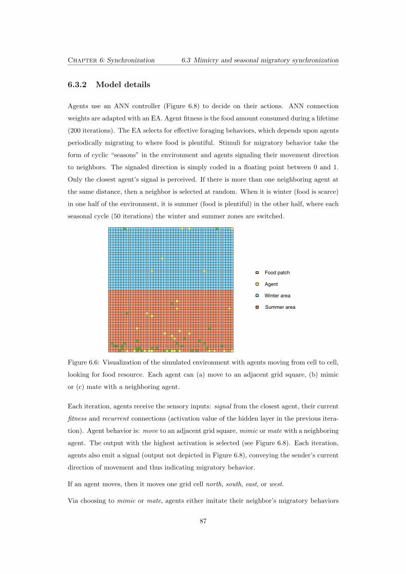
Chapter 6: Synchronization 6.3 Mimicry and seasonal migratory synchronization
6.3.2 Model details
Agents use an ANN controller (Figure 6.8) to decide on their actions. ANN connection
weights are adapted with an EA. Agent fitness is the food amount consumed during a lifetime
(200 iterations). The EA selects for e↵ective foraging behaviors, which depends upon agents
periodically migrating to where food is plentiful. Stimuli for migratory behavior take the
form of cyclic “seasons” in the environment and agents signaling their movement direction
to neighbors. The signaled direction is simply coded in a floating point between 0 and 1.
Only the closest agent’s signal is perceived. If there is more than one neighboring agent at
the same distance, then a neighbor is selected at random. When it is winter (food is scarce)
in one half of the environment, it is summer (food is plentiful) in the other half, where each
seasonal cycle (50 iterations) the winter and summer zones are switched.
Food patch
Agent
Winter area
Summer area
Figure 6.6: Visualization of the simulated environment with agents moving from cell to cell,
looking for food resource. Each agent can (a) move to an adjacent grid square, (b) mimic
or (c) mate with a neighboring agent.
Each iteration, agents receive the sensory inputs: signal from the closest agent, their current
fitness and recurrent connections (activation value of the hidden layer in the previous itera-
tion). Agent behavior is: move to an adjacent grid square, mimic or mate with a neighboring
agent. The output with the highest activation is selected (see Figure 6.8). Each iteration,
agents also emit a signal (output not depicted in Figure 6.8), conveying the sender’s current
direction of movement and thus indicating migratory behavior.
If an agent moves, then it moves one grid cell north, south, east, or west.
Via choosing to mimic or mate, agents either imitate their neighbor’s migratory behaviors
87
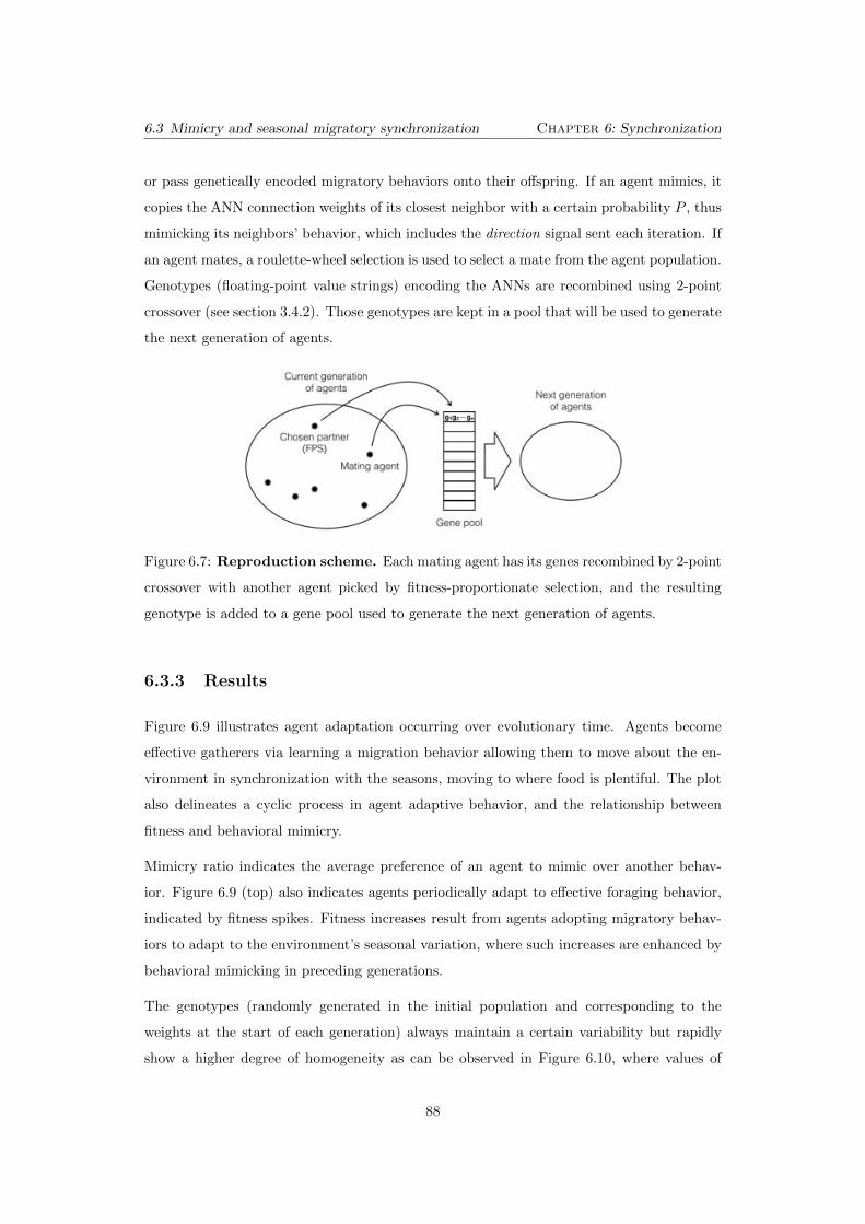
6.3 Mimicry and seasonal migratory synchronization Chapter 6: Synchronization
or pass genetically encoded migratory behaviors onto their o↵spring. If an agent mimics, it
copies the ANN connection weights of its closest neighbor with a certain probability P , thus
mimicking its neighbors’ behavior, which includes the direction signal sent each iteration. If
an agent mates, a roulette-wheel selection is used to select a mate from the agent population.
Genotypes (floating-point value strings) encoding the ANNs are recombined using 2-point
crossover (see section 3.4.2). Those genotypes are kept in a pool that will be used to generate
the next generation of agents.
Figure 6.7: Reproduction scheme. Each mating agent has its genes recombined by 2-point
crossover with another agent picked by fitness-proportionate selection, and the resulting
genotype is added to a gene pool used to generate the next generation of agents.
6.3.3 Results
Figure 6.9 illustrates agent adaptation occurring over evolutionary time. Agents become
e↵ective gatherers via learning a migration behavior allowing them to move about the en-
vironment in synchronization with the seasons, moving to where food is plentiful. The plot
also delineates a cyclic process in agent adaptive behavior, and the relationship between
fitness and behavioral mimicry.
Mimicry ratio indicates the average preference of an agent to mimic over another behav-
ior. Figure 6.9 (top) also indicates agents periodically adapt to e↵ective foraging behavior,
indicated by fitness spikes. Fitness increases result from agents adopting migratory behav-
iors to adapt to the environment’s seasonal variation, where such increases are enhanced by
behavioral mimicking in preceding generations.
The genotypes (randomly generated in the initial population and corresponding to the
weights at the start of each generation) always maintain a certain variability but rapidly
show a higher degree of homogeneity as can be observed in Figure 6.10, where values of
88
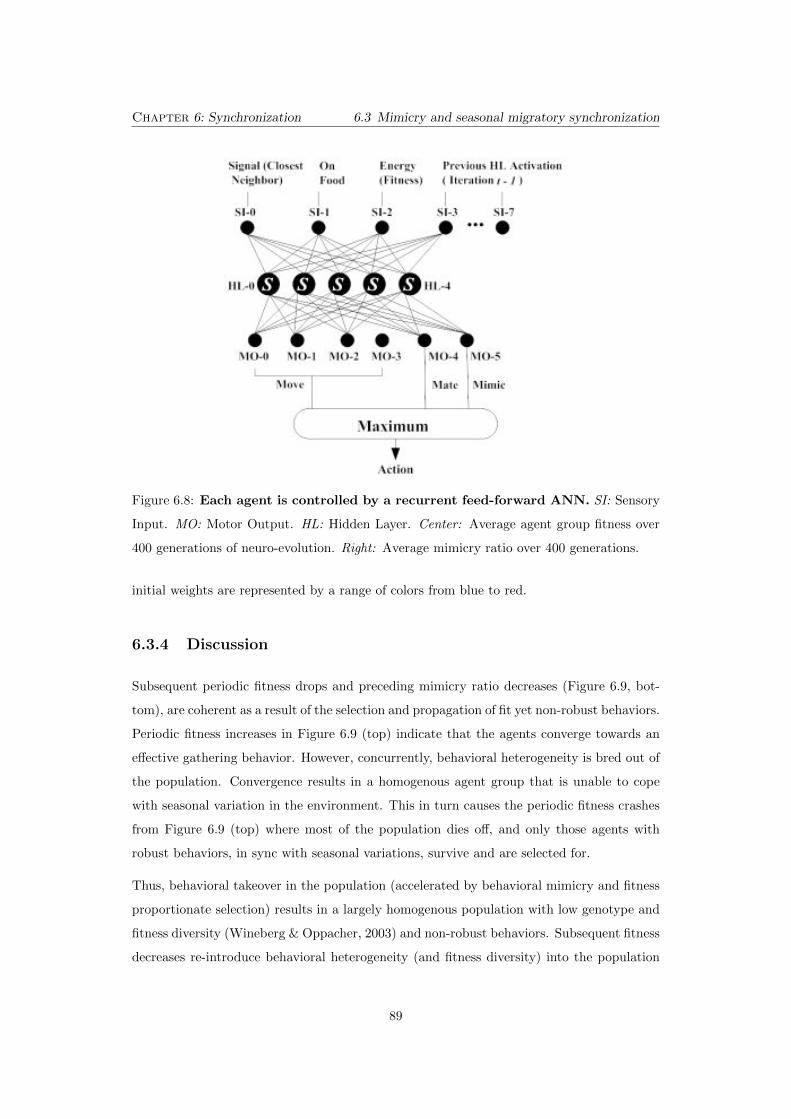
Chapter 6: Synchronization 6.3 Mimicry and seasonal migratory synchronization
Figure 6.8: Each agent is controlled by a recurrent feed-forward ANN. SI: Sensory
Input. MO: Motor Output. HL: Hidden Layer. Center: Average agent group fitness over
400 generations of neuro-evolution. Right: Average mimicry ratio over 400 generations.
initial weights are represented by a range of colors from blue to red.
6.3.4 Discussion
Subsequent periodic fitness drops and preceding mimicry ratio decreases (Figure 6.9, bot-
tom), are coherent as a result of the selection and propagation of fit yet non-robust behaviors.
Periodic fitness increases in Figure 6.9 (top) indicate that the agents converge towards an
e↵ective gathering behavior. However, concurrently, behavioral heterogeneity is bred out of
the population. Convergence results in a homogenous agent group that is unable to cope
with seasonal variation in the environment. This in turn causes the periodic fitness crashes
from Figure 6.9 (top) where most of the population dies o↵, and only those agents with
robust behaviors, in sync with seasonal variations, survive and are selected for.
Thus, behavioral takeover in the population (accelerated by behavioral mimicry and fitness
proportionate selection) results in a largely homogenous population with low genotype and
fitness diversity (Wineberg & Oppacher, 2003) and non-robust behaviors. Subsequent fitness
decreases re-introduce behavioral heterogeneity (and fitness diversity) into the population
89
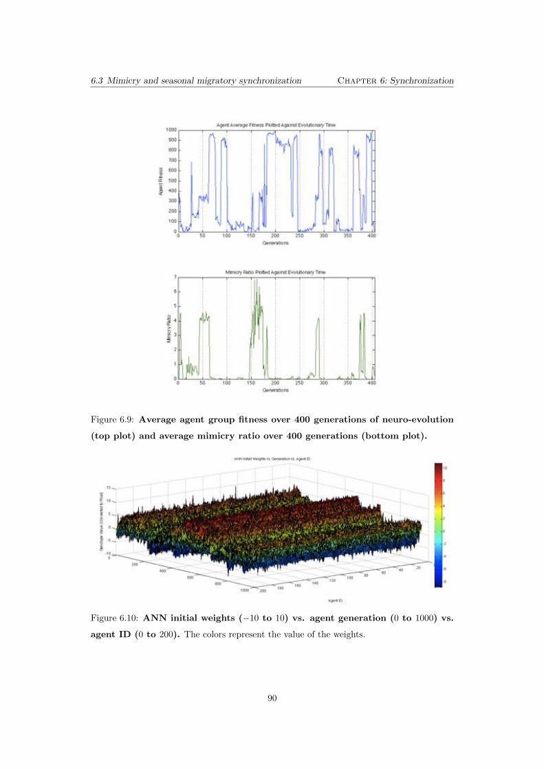
6.3 Mimicry and seasonal migratory synchronization Chapter 6: Synchronization
Figure 6.9: Average agent group fitness over 400 generations of neuro-evolution
(top plot) and average mimicry ratio over 400 generations (bottom plot).
Figure 6.10: ANN initial weights (�10 to 10) vs. agent generation (0 to 1000) vs.
agent ID (0 to 200). The colors represent the value of the weights.
90
Chapter 6: Synchronization 6.4 Size-dependent saving strategies
and allow agents to re-adapt to the environment’s seasonal variation via adopting a migratory
behavior. Figure 6.9 also indicates that variations in the mimicry rate impact the rate of
agent adaptation and re-adaptation, as well as the duration of fitness spikes. That is,
fitness increases are correlated with high mimicry ratios and fitness crashes cause behaviors
containing the propensity to mimic to be periodically lost, and then rediscovered in the
subsequent re-adaptation phase.
The modeling of mimicry itself by a probability of weight copy in ANNs is quite an over-
simplification of the mimicry studied in biology. However, we argue that this approach is
suitable to the purposes of the minimalist model presented here.
The results indicate the importance of behavioral mimicry and genetic transmission of mi-
gratory behaviors to a population’s overall adaptivity, supporting ethological research. How-
ever, their contribution to adaptive behavior is still subject to ongoing research, to study the
conditions under which cultural versus genetic transmission of migratory behaviors prevail,
and the impact of lifetime duration on cultural and genetic transmission of behaviors.
This second study of the chapter again shows a synchronization of the agents’ behavior based
on the signals they exchange, eventually allowing them to improve their foraging based on
a migration-like behavior. This constitutes a second strategy for the agents to save energy,
to overcome the seasonal change. It should be noted that although the specific focus on
imitation and conformity is not explored further in this chapter, it will be treated further
in Chapter 7, where it truly plays a central part of the model.
6.4 Periodic resource scarcity leads to size-dependent
saving strategies
This section studies the behavior of populations of foraging agents facing resource variation in
time, while interacting only through resource consumption. The results show the emergence
of various size dependent strategies, among which is found resource saving behavior, also
known as hoarding.
91
6.4 Size-dependent saving strategies Chapter 6: Synchronization
6.4.1 Hoarding behavior
Hoarding is the act of storing a resource without any plan to use it in a foreseeable future,
and has been shown to be a viable, adaptive behavior (Andersson & Krebs, 1978; Smulders,
1998).
A significant amount of e↵ort has been made to understand pilferage control and tolerance
(Clarke & Kramer, 1994; Vander Wall & Jenkins, 2003; Ekman et al., 1996). In addition,
many of those models study cache spacing (Kraus, 1983) and collective hoarding (Bardin &
Markovets, 1991; Brodin & Ekman, 1994). However, Andersson & Krebs (1978) show that
reciprocal pilfering can make hoarding systems resilient to invasions of cheaters, and argue
that the hoarding behavior does not need to be considered as an altruistic mechanism. Most
of the research on food-hoarding has disregarded the influence of primary factors such as
distribution of food over time or the consequences of agents’ size on their caching behavior.
This is the point where the modelling facet of Artificial Life may bring new highlights on
hoarding behavior.
This research investigates the impact of changes in environment resources, available to a pop-
ulation of individuals, on their caching strategy. To do so, we present a simple agent-based
model incorporating a population of individuals capable of storing resources, adapting their
behavior through generations, in a world o↵ering a di↵erentiated cyclic food distribution.
6.4.2 Model
Our model is based on agents striving to obtain food from the environment. They are
given five possible actions: eat, forage, store food, reproduce or do nothing. The decision
mechanism is implemented by an artificial neural network with inputs set to food availability
(“temperature”), current energy of the agent (“hunger”) and result of the last forage. We
also feedback the results of the cached layer to give the agent some kind of memory.
The weights of the neural network, randomized at first, are refined through mutations and
crossovers on the span of multiple generations. The genotype also determines the agent’s
size, that influences the cost of its actions. In the genotype, each weight is coded by one
floating point value, while the size is represented by 10 values. The genotype is evolved
through an evolutionary algorithm (EA), with a two-point crossover and a 5% mutation
rate.
92
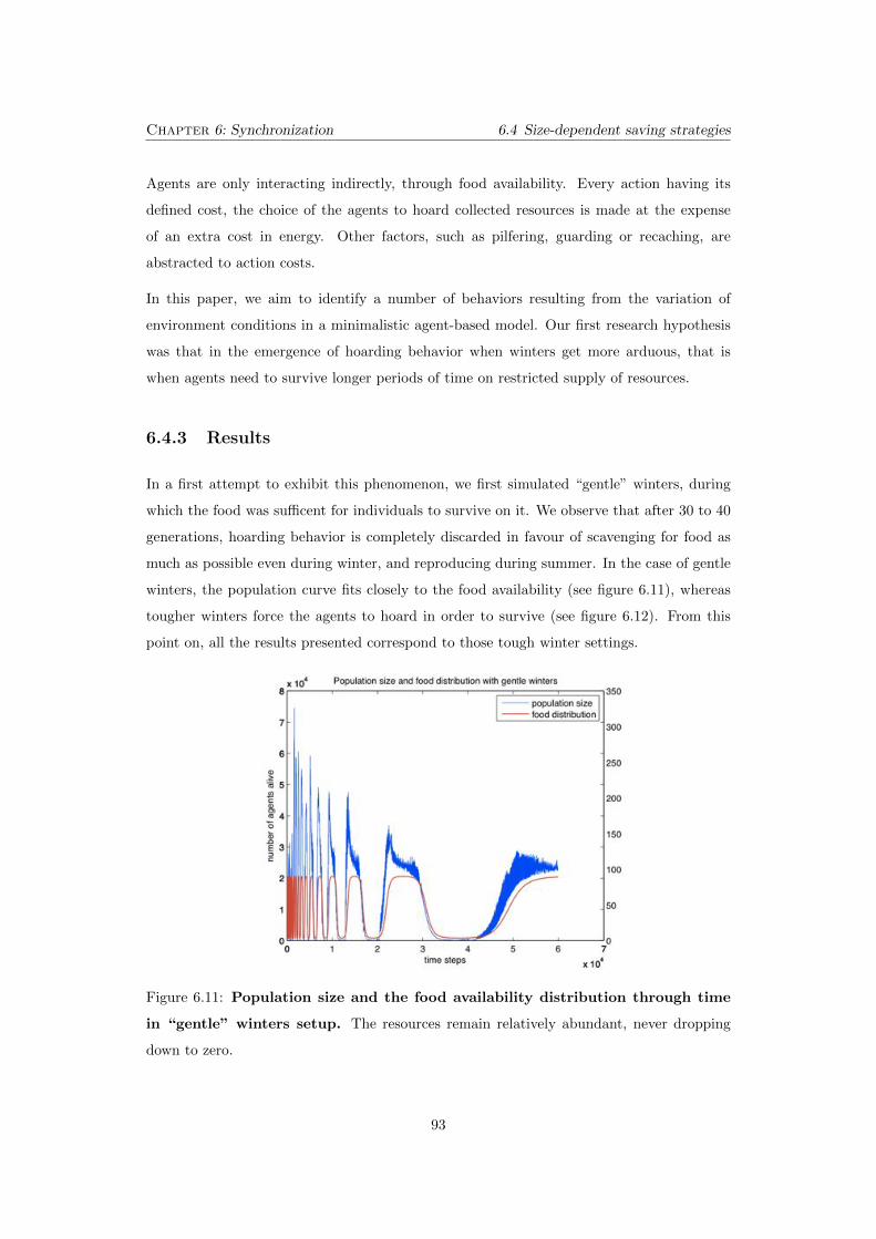
Chapter 6: Synchronization 6.4 Size-dependent saving strategies
Agents are only interacting indirectly, through food availability. Every action having its
defined cost, the choice of the agents to hoard collected resources is made at the expense
of an extra cost in energy. Other factors, such as pilfering, guarding or recaching, are
abstracted to action costs.
In this paper, we aim to identify a number of behaviors resulting from the variation of
environment conditions in a minimalistic agent-based model. Our first research hypothesis
was that in the emergence of hoarding behavior when winters get more arduous, that is
when agents need to survive longer periods of time on restricted supply of resources.
6.4.3 Results
In a first attempt to exhibit this phenomenon, we first simulated “gentle” winters, during
which the food was su�cent for individuals to survive on it. We observe that after 30 to 40
generations, hoarding behavior is completely discarded in favour of scavenging for food as
much as possible even during winter, and reproducing during summer. In the case of gentle
winters, the population curve fits closely to the food availability (see figure 6.11), whereas
tougher winters force the agents to hoard in order to survive (see figure 6.12). From this
point on, all the results presented correspond to those tough winter settings.
Figure 6.11: Population size and the food availability distribution through time
in “gentle” winters setup. The resources remain relatively abundant, never dropping
down to zero.
93
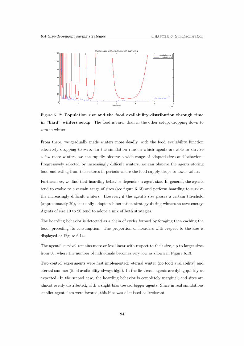
6.4 Size-dependent saving strategies Chapter 6: Synchronization
0 1 2 3 4 5 6
x 104
0
20
40
60
80
100
120Population size and food distribution with tough winters
time steps
population sizefood distribution
Figure 6.12: Population size and the food availability distribution through time
in “hard” winters setup. The food is rarer than in the other setup, dropping down to
zero in winter.
From there, we gradually made winters more deadly, with the food availability function
e↵ectively dropping to zero. In the simulation runs in which agents are able to survive
a few more winters, we can rapidly observe a wide range of adapted sizes and behaviors.
Progressively selected by increasingly di�cult winters, we can observe the agents storing
food and eating from their stores in periods where the food supply drops to lower values.
Furthermore, we find that hoarding behavior depends on agent size. In general, the agents
tend to evolve to a certain range of sizes (see figure 6.13) and perform hoarding to survive
the increasingly di�cult winters. However, if the agent’s size passes a certain threshold
(approximately 20), it usually adopts a hibernation strategy during winters to save energy.
Agents of size 10 to 20 tend to adopt a mix of both strategies.
The hoarding behavior is detected as a chain of cycles formed by foraging then caching the
food, preceding its consumption. The proportion of hoarders with respect to the size is
displayed at Figure 6.14.
The agents’ survival remains more or less linear with respect to their size, up to larger sizes
from 50, where the number of individuals becomes very low as shown in Figure 6.13.
Two control experiments were first implemented: eternal winter (no food availability) and
eternal summer (food availability always high). In the first case, agents are dying quickly as
expected. In the second case, the hoarding behavior is completely marginal, and sizes are
almost evenly distributed, with a slight bias toward bigger agents. Since in real simulations
smaller agent sizes were favored, this bias was dismissed as irrelevant.
94
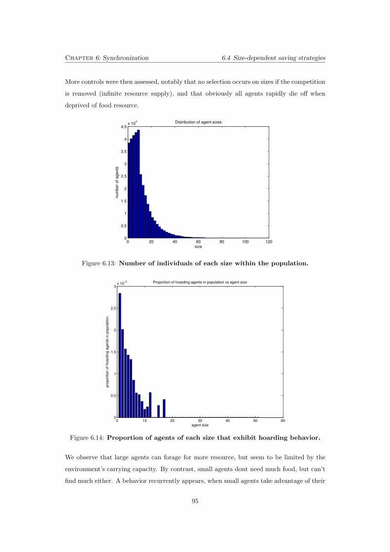
Chapter 6: Synchronization 6.4 Size-dependent saving strategies
More controls were then assessed, notably that no selection occurs on sizes if the competition
is removed (infinite resource supply), and that obviously all agents rapidly die o↵ when
deprived of food resource.
0 20 40 60 80 100 1200
0.5
1
1.5
2
2.5
3
3.5
4
4.5x 10
4 Distribution of agent sizes
num
ber
of agents
size
Figure 6.13: Number of individuals of each size within the population.
0 10 20 30 40 50 600
0.5
1
1.5
2
2.5
3x 10
−3
agent size
pro
po
rtio
n o
f h
oa
rdin
g a
ge
nts
in p
op
ula
tion
Proportion of hoarding agents in population vs agent size
Figure 6.14: Proportion of agents of each size that exhibit hoarding behavior.
We observe that large agents can forage for more resource, but seem to be limited by the
environment’s carrying capacity. By contrast, small agents dont need much food, but can’t
find much either. A behavior recurrently appears, when small agents take advantage of their
95
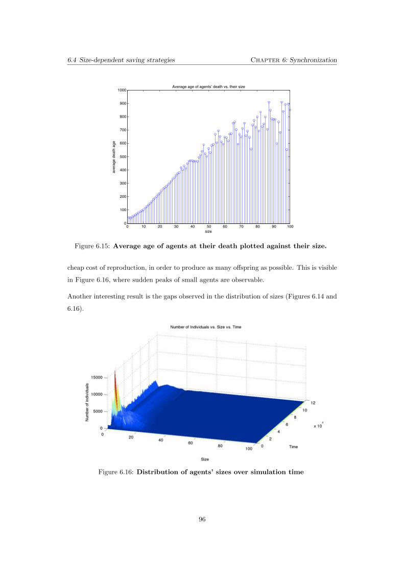
6.4 Size-dependent saving strategies Chapter 6: Synchronization
0 10 20 30 40 50 60 70 80 90 1000
100
200
300
400
500
600
700
800
900
1000
size
aver
age
deat
h ag
e
Average age of agents’ death vs. their size
Figure 6.15: Average age of agents at their death plotted against their size.
cheap cost of reproduction, in order to produce as many o↵spring as possible. This is visible
in Figure 6.16, where sudden peaks of small agents are observable.
Another interesting result is the gaps observed in the distribution of sizes (Figures 6.14 and
6.16).
Figure 6.16: Distribution of agents’ sizes over simulation time
96
Chapter 6: Synchronization 6.4 Size-dependent saving strategies
6.4.4 Discussion
The indirect interaction of the agents in the model presented in this section contrasts with
the fixed-value signals exchanged in Section 6.2 and the free signals exchanged with close
neighbors in Section 6.3. In the absence of such solutions, the only possible adaptation is
to directly optimize one’s behavior to the fluctuations of the environment, and that is what
is observed in this model.
The agents develop a hoarding behavior that enables them to survive in sometimes easy,
sometimes extreme conditions, using the available solutions to them in a way similar to
what is observed in behavioral ecology (Andersson & Krebs, 1978; Bardin & Markovets,
1991; Brodin & Ekman, 1994).
The behavior involving small agents taking advantage of their cheap reproduction cost can
be related to a known phenomenon in mathematical biology. This strategy of survival
focusing on the quantity of progeny over its quality, typically adopted by bacteria or insects,
is referred to as an “r-strategy” (MacArthur and Wilson, 1967). The emergence of this so-
called “r/K” opposition visibly demands no more than simplistic laboratory settings such
as our model. These concepts have recently regained interest in panarchy theories and
age-specific mortality (Gunderson, 2001; Reznick et al., 2002; Sabeti et al., 2007).
Whether our hypotheses are compatible with other r/K characteristics is still to be examined
further, notably by looking in more detail at a limited number of o↵spring. Besides, more
action choices can be given to the modeled agents, such as the ability to share food, in order
to let more K behaviors emerge.
Our results indicate that the agents’ size and the environment time cycles are major factors
influencing their behavior, as may be observed in nature. This also suggests that our model
could somewhat predict behavior modification to adapt to di↵erent conditions, such as
abnormally long winters.
Finally, our model produces gaps, observed in the distribution of sizes. This unexpected
result may be due to the formation of local attractors for particular sizes in the system, and
could benefit from a larger scale analysis, to shed light on eventual unknown e↵ects linked
to the emergence of hoarding behavior.
This model can be considered as a control experiment to the two first works of this chapter.
The agents’ interaction is limited to resource consumption, letting the system develop opti-
mizations based on the remaining cards available, i.e. the optimization through the choice
97

6.4 Size-dependent saving strategies Chapter 6: Synchronization
of optimal sequences of actions, which are the di↵erent cycles of actions we have detected,
that agents use as saving strategies in variable resource environments.
98
Chapter7Neutral selection in gene-culture coevolu-
tion
In the study of biocultural evolution, human behavior is the product of two di↵erent and
interacting evolutionary processes: genetic and cultural evolution. The dual-inheritance
theory (DIT) defines culture as information and behavior acquired through social learning,
and claims that this culture evolves through a process analogous, although not identical, to
genetic evolution (Lumsden & Wilson, 1981; Boyd & Richerson, 1992; Richerson & Boyd,
2008). As genetic evolution is relatively well understood, the DIT focuses on cultural evo-
lution and the interactions between cultural evolution and genetic evolution.
One example of the recurrent objects of study of the theory is the controversial Baldwin
e↵ect (Baldwin, 1896; Simpson, 1953; Weber & Depew, 2003), which states that unlearned
can replace learned behavior. This e↵ect has been specifically applied to the evolution of
language (Munroe & Cangelosi, 2002; Deacon, 2003a; Christiansen & Kirby, 2003), which
will be of interest in this chapter.
Yamauchi & Hashimoto (2010) have introduced a computational model of gene-culture co-
evolution to investigate that very Baldwin e↵ect. This type of computational simulation
takes a special importance in language evolution, due to the lack of empirical data. Unfor-
tunately, although the study presents powerful results, a large part of the behaviors reported
in the model turned out to be artifacts produced by the specific design and set of parameters
(McCrohon & Witkowski, 2011).
In this chapter, after a short review of the area, we present a new gene-culture model, in the
hope to demonstrate specific dynamics without the hidden biases present in the previous
model. Adapting once again the ABM approach presented in the previous chapters, we
improve on the simulation of the agent controller’s architecture, the cultural landscape and
99
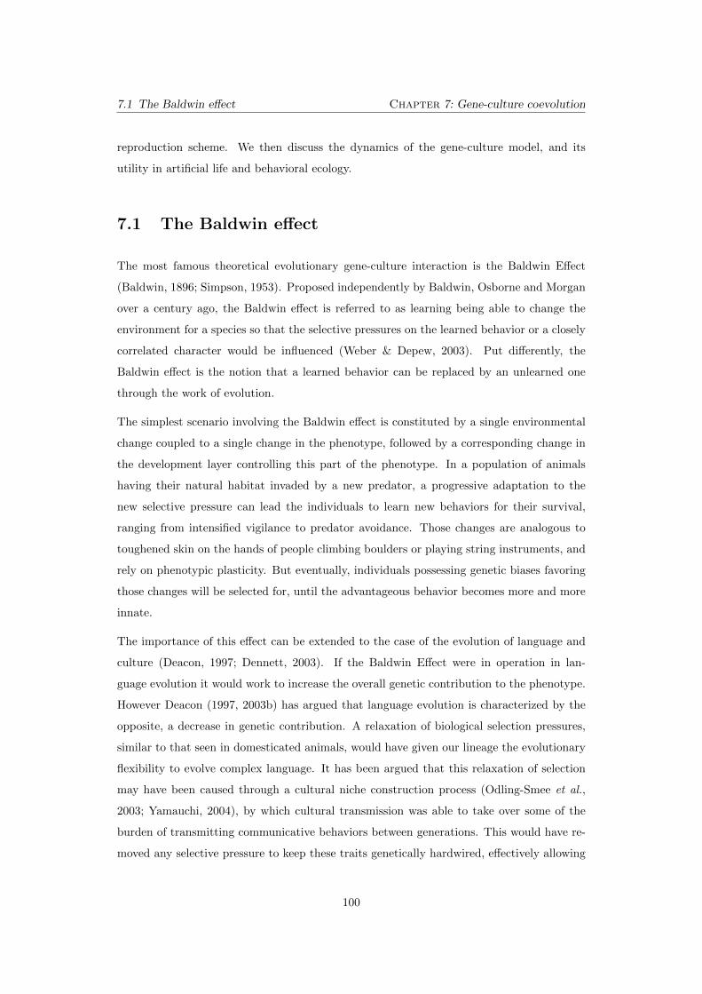
7.1 The Baldwin e↵ect Chapter 7: Gene-culture coevolution
reproduction scheme. We then discuss the dynamics of the gene-culture model, and its
utility in artificial life and behavioral ecology.
7.1 The Baldwin e↵ect
The most famous theoretical evolutionary gene-culture interaction is the Baldwin E↵ect
(Baldwin, 1896; Simpson, 1953). Proposed independently by Baldwin, Osborne and Morgan
over a century ago, the Baldwin e↵ect is referred to as learning being able to change the
environment for a species so that the selective pressures on the learned behavior or a closely
correlated character would be influenced (Weber & Depew, 2003). Put di↵erently, the
Baldwin e↵ect is the notion that a learned behavior can be replaced by an unlearned one
through the work of evolution.
The simplest scenario involving the Baldwin e↵ect is constituted by a single environmental
change coupled to a single change in the phenotype, followed by a corresponding change in
the development layer controlling this part of the phenotype. In a population of animals
having their natural habitat invaded by a new predator, a progressive adaptation to the
new selective pressure can lead the individuals to learn new behaviors for their survival,
ranging from intensified vigilance to predator avoidance. Those changes are analogous to
toughened skin on the hands of people climbing boulders or playing string instruments, and
rely on phenotypic plasticity. But eventually, individuals possessing genetic biases favoring
those changes will be selected for, until the advantageous behavior becomes more and more
innate.
The importance of this e↵ect can be extended to the case of the evolution of language and
culture (Deacon, 1997; Dennett, 2003). If the Baldwin E↵ect were in operation in lan-
guage evolution it would work to increase the overall genetic contribution to the phenotype.
However Deacon (1997, 2003b) has argued that language evolution is characterized by the
opposite, a decrease in genetic contribution. A relaxation of biological selection pressures,
similar to that seen in domesticated animals, would have given our lineage the evolutionary
flexibility to evolve complex language. It has been argued that this relaxation of selection
may have been caused through a cultural niche construction process (Odling-Smee et al.,
2003; Yamauchi, 2004), by which cultural transmission was able to take over some of the
burden of transmitting communicative behaviors between generations. This would have re-
moved any selective pressure to keep these traits genetically hardwired, e↵ectively allowing
100
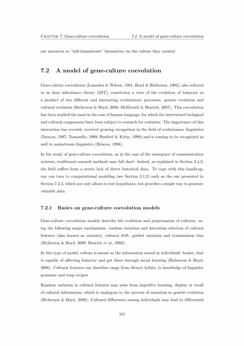
Chapter 7: Gene-culture coevolution 7.2 A model of gene-culture coevolution
our ancestors to “self-domesticate” themselves via the culture they created.
7.2 A model of gene-culture coevolution
Gene-culture coevolution (Lumsden & Wilson, 1981; Boyd & Richerson, 1992), also referred
to as dual inheritance theory (DIT), constitutes a view of the evolution of behavior as
a product of two di↵erent and interacting evolutionary processes: genetic evolution and
cultural evolution (Richerson & Boyd, 2008; McElreath & Henrich, 2007). This coevolution
has been studied the most in the case of human language, for which the intertwined biological
and cultural components have been subject to research for centuries. The importance of this
interaction has recently received growing recognition in the field of evolutionary linguistics
(Deacon, 1997; Tomasello, 1999; Hurford & Kirby, 1999) and is coming to be recognized as
well in mainstream linguistics (Briscoe, 1998).
In the study of gene-culture coevolution, as in the case of the emergence of communication
systems, traditional research methods may fall short. Indeed, as explained in Section 2.4.2,
the field su↵ers from a severe lack of direct historical data. To cope with this handicap,
one can turn to computational modeling (see Section 3.1.2) such as the one presented in
Section 7.2.2, which not only allows to test hypotheses, but provides a simple way to generate
valuable data.
7.2.1 Basics on gene-culture coevolution models
Gene-culture coevolution models describe the evolution and perpetuation of cultures, us-
ing the following major mechanisms: random variation and darwinian selection of cultural
features (also known as variants), cultural drift, guided variation and transmission bias
(Richerson & Boyd, 2008; Henrich et al., 2008).
In this type of model, culture is meant as the information stored in individuals’ brains, that
is capable of a↵ecting behavior and got there through social learning (Richerson & Boyd,
2008). Cultural features can therefore range from dietary habits, to knowledge of linguistic
grammar and soup recipes.
Random variation in cultural features may arise from imperfect learning, display or recall
of cultural information, which is analogous to the process of mutation in genetic evolution
(Richerson & Boyd, 2008). Cultural di↵erences among individuals may lead to di↵erential
101
7.2 A model of gene-culture coevolution Chapter 7: Gene-culture coevolution
survival of individuals. The patterns of this selective process depend on transmission biases
and can result in behavior that is more adaptive to a given environment. In cultural drift,
analogous to genetic drift in evolutionary biology (Bentley et al., 2004), the frequency of
cultural traits in a population may be subject to random variations, causing cultural features
to disappear from a population. This e↵ect should be especially strong in small populations.
Cultural traits are gained in a population through learning, novel traits being transmitted
to other members of the population. This process of guided variation depends on an adap-
tive standard that determines which cultural variants are learned. Culture traits can be
transmitted between individuals in di↵erent ways. The so-called transmission biases occur
whenever some features are favored over others in the process of cultural transmission. The
biases can be of di↵erent types, linked to their content, context, individual (or model-based)
or conformity (more generally frequency-dependent) (Henrich & McElreath, 2003).
7.2.2 Repeated masking and unmasking of natural selection
Yamauchi & Hashimoto (2010) presents a computational model designed to investigate the
gene-culture coevolution. The model claims to show a cyclic repetition of stages in which
biological selection is masked by cultural evolution, before being vigorously reasserted. More
specifically, the three successive stages are the Baldwin e↵ect, the functional redundancy and
the unmasking of natural selection.
The progression of gene-grammar match1 is depicted in Figure 7.1. The learning intensity2 is
shown in Figure 7.2. This type of cycle has not been attested clearly in empirical data. This
may indeed be the product of an artificially high rate of simulated biological evolution when
compared with the rate of cultural change, as suggested by Chater et al. (2009), arguing
that faster rates of culture change provide a moving target that biological evolution has a
hard time adapting to.
However, McCrohon & Witkowski (2011) show that the model’s apparent cyclic behavior
can be better described as a random walk between a linearly ordered set of attractor states
(see Figure 7.3), as a result of arbitrarily chosen model parameter settings. The original
conclusions therefore lie on artifactual dynamics, which challenges the claim for cyclic stages
of shielding and unmasking.
1the average hamming distance between mature agents’ grammars and chromosomes2the average amount of learning resource consumed by agents in the learning phase
102
Chapter 7: Gene-culture coevolution 7.3 Remarkable features of the model
Figure 7.1: Gene-Grammar Matches (based on the original model from Yamauchi &
Hashimoto (2010), reproduced in McCrohon & Witkowski (2011)) [Seed=1303050913721,
Runs=1, Generations=5000]
Figure 7.2: Number of Genotypes (based on the original model from Yamauchi &
Hashimoto (2010), reproduced in McCrohon & Witkowski (2011)) [Seed=1303050913721,
Runs=1, Generations=5000]
In the next section, we present a model improving on the original design, able to show
special dynamics in the gene-culture dynamics. In particular, we introduce new agent con-
trollers, incorporate contrasted gene-culture landscapes, get rid of discrete parametrization
and augment the agent population’s scale.
7.3 Remarkable features of the model
We now introduce a series of drastic changes in the model presented previously, based on
Yamauchi & Hashimoto (2010), in order to build a robust model of gene-culture coevolution.
In the following, we justify every change and analyze the results.
103
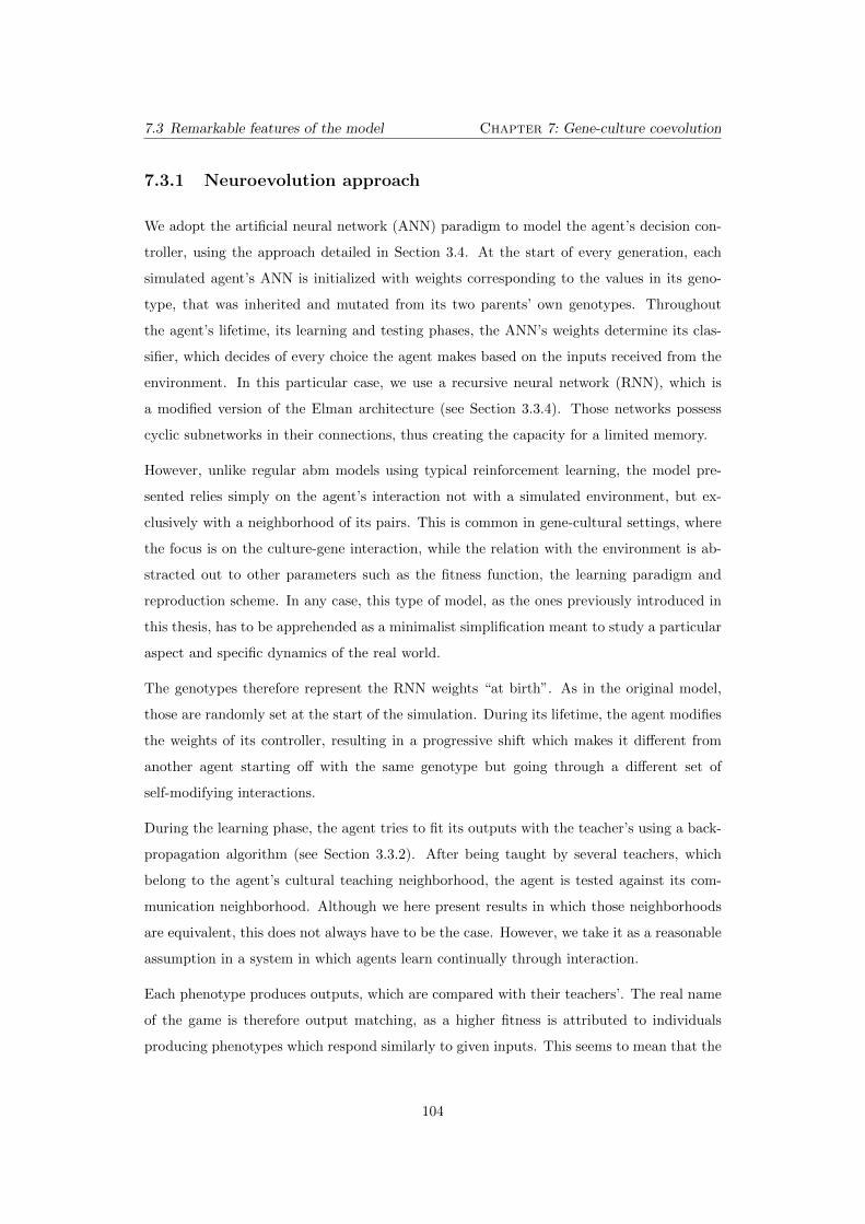
7.3 Remarkable features of the model Chapter 7: Gene-culture coevolution
7.3.1 Neuroevolution approach
We adopt the artificial neural network (ANN) paradigm to model the agent’s decision con-
troller, using the approach detailed in Section 3.4. At the start of every generation, each
simulated agent’s ANN is initialized with weights corresponding to the values in its geno-
type, that was inherited and mutated from its two parents’ own genotypes. Throughout
the agent’s lifetime, its learning and testing phases, the ANN’s weights determine its clas-
sifier, which decides of every choice the agent makes based on the inputs received from the
environment. In this particular case, we use a recursive neural network (RNN), which is
a modified version of the Elman architecture (see Section 3.3.4). Those networks possess
cyclic subnetworks in their connections, thus creating the capacity for a limited memory.
However, unlike regular abm models using typical reinforcement learning, the model pre-
sented relies simply on the agent’s interaction not with a simulated environment, but ex-
clusively with a neighborhood of its pairs. This is common in gene-cultural settings, where
the focus is on the culture-gene interaction, while the relation with the environment is ab-
stracted out to other parameters such as the fitness function, the learning paradigm and
reproduction scheme. In any case, this type of model, as the ones previously introduced in
this thesis, has to be apprehended as a minimalist simplification meant to study a particular
aspect and specific dynamics of the real world.
The genotypes therefore represent the RNN weights “at birth”. As in the original model,
those are randomly set at the start of the simulation. During its lifetime, the agent modifies
the weights of its controller, resulting in a progressive shift which makes it di↵erent from
another agent starting o↵ with the same genotype but going through a di↵erent set of
self-modifying interactions.
During the learning phase, the agent tries to fit its outputs with the teacher’s using a back-
propagation algorithm (see Section 3.3.2). After being taught by several teachers, which
belong to the agent’s cultural teaching neighborhood, the agent is tested against its com-
munication neighborhood. Although we here present results in which those neighborhoods
are equivalent, this does not always have to be the case. However, we take it as a reasonable
assumption in a system in which agents learn continually through interaction.
Each phenotype produces outputs, which are compared with their teachers’. The real name
of the game is therefore output matching, as a higher fitness is attributed to individuals
producing phenotypes which respond similarly to given inputs. This seems to mean that the
104
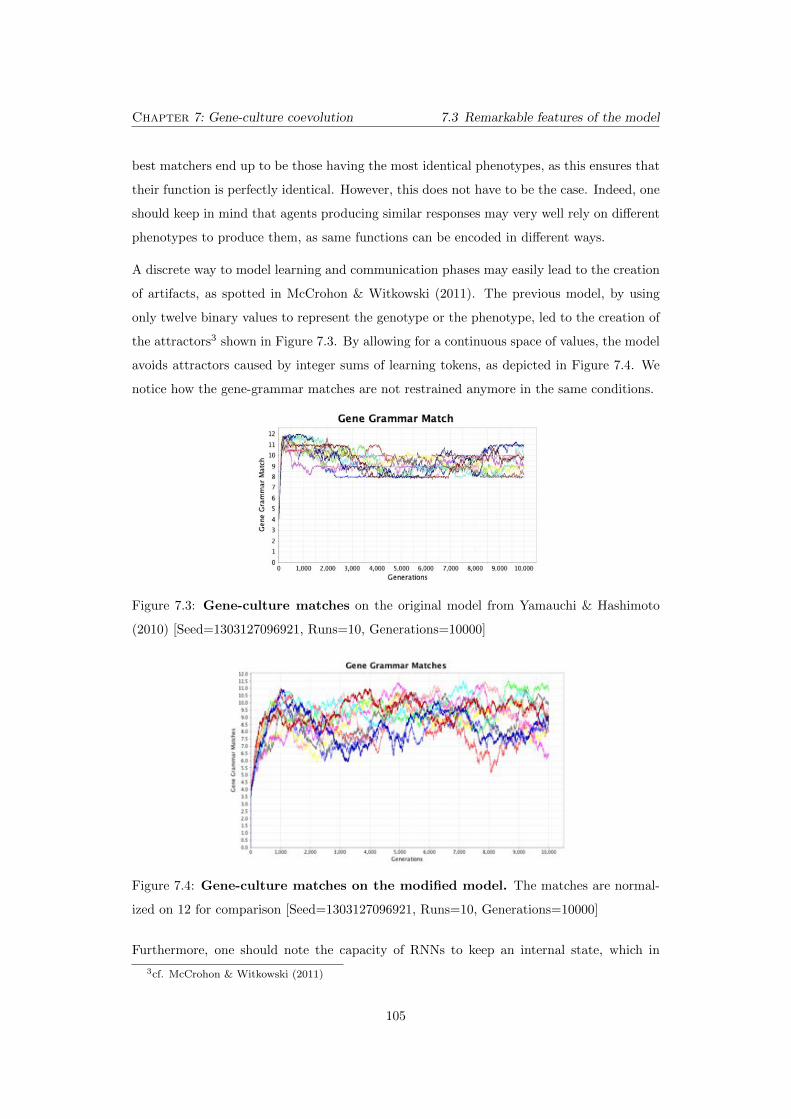
Chapter 7: Gene-culture coevolution 7.3 Remarkable features of the model
best matchers end up to be those having the most identical phenotypes, as this ensures that
their function is perfectly identical. However, this does not have to be the case. Indeed, one
should keep in mind that agents producing similar responses may very well rely on di↵erent
phenotypes to produce them, as same functions can be encoded in di↵erent ways.
A discrete way to model learning and communication phases may easily lead to the creation
of artifacts, as spotted in McCrohon & Witkowski (2011). The previous model, by using
only twelve binary values to represent the genotype or the phenotype, led to the creation of
the attractors3 shown in Figure 7.3. By allowing for a continuous space of values, the model
avoids attractors caused by integer sums of learning tokens, as depicted in Figure 7.4. We
notice how the gene-grammar matches are not restrained anymore in the same conditions.
Figure 7.3: Gene-culture matches on the original model from Yamauchi & Hashimoto
(2010) [Seed=1303127096921, Runs=10, Generations=10000]
Figure 7.4: Gene-culture matches on the modified model. The matches are normal-
ized on 12 for comparison [Seed=1303127096921, Runs=10, Generations=10000]
Furthermore, one should note the capacity of RNNs to keep an internal state, which in
3cf. McCrohon & Witkowski (2011)
105
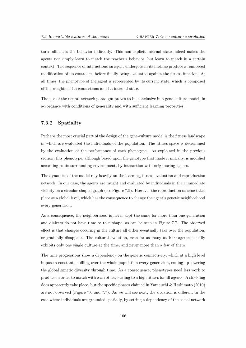
7.3 Remarkable features of the model Chapter 7: Gene-culture coevolution
turn influences the behavior indirectly. This non-explicit internal state indeed makes the
agents not simply learn to match the teacher’s behavior, but learn to match in a certain
context. The sequence of interactions an agent undergoes in its lifetime produce a reinforced
modification of its controller, before finally being evaluated against the fitness function. At
all times, the phenotype of the agent is represented by its current state, which is composed
of the weights of its connections and its internal state.
The use of the neural network paradigm proves to be conclusive in a gene-culture model, in
accordance with conditions of generality and with su�cient learning properties.
7.3.2 Spatiality
Perhaps the most crucial part of the design of the gene-culture model is the fitness landscape
in which are evaluated the individuals of the population. The fitness space is determined
by the evaluation of the performance of each phenotype. As explained in the previous
section, this phenotype, although based upon the genotype that made it initially, is modified
according to its surrounding environment, by interaction with neighboring agents.
The dynamics of the model rely heavily on the learning, fitness evaluation and reproduction
network. In our case, the agents are taught and evaluated by individuals in their immediate
vicinity on a circular-shaped graph (see Figure 7.5). However the reproduction scheme takes
place at a global level, which has the consequence to change the agent’s genetic neighborhood
every generation.
As a consequence, the neighborhood is never kept the same for more than one generation
and dialects do not have time to take shape, as can be seen in Figure 7.7. The observed
e↵ect is that changes occuring in the culture all either eventually take over the population,
or gradually disappear. The cultural evolution, even for as many as 1000 agents, usually
exhibits only one single culture at the time, and never more than a few of them.
The time progressions show a dependency on the genetic connectivity, which at a high level
impose a constant shu✏ing over the whole population every generation, ending up lowering
the global genetic diversity through time. As a consequence, phenotypes need less work to
produce in order to match with each other, leading to a high fitness for all agents. A shielding
does apparently take place, but the specific phases claimed in Yamauchi & Hashimoto (2010)
are not observed (Figure 7.6 and 7.7). As we will see next, the situation is di↵erent in the
case where individuals are grounded spatially, by setting a dependency of the social network
106
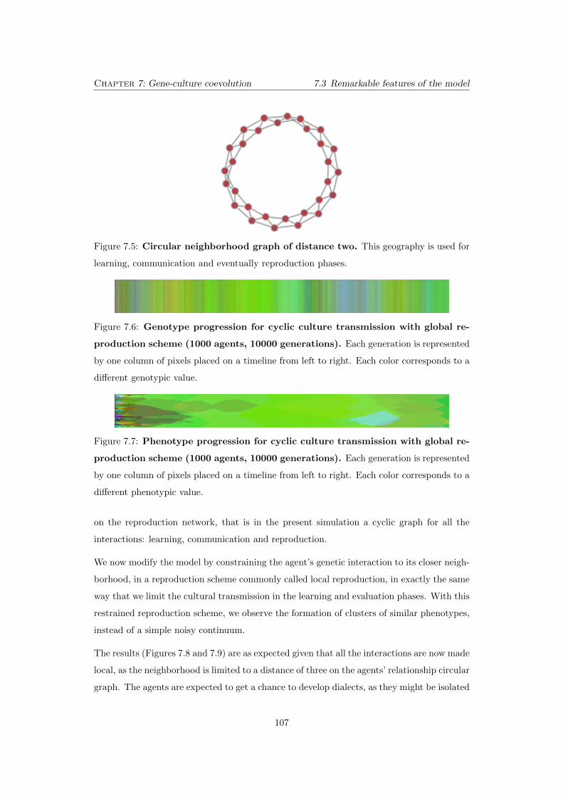
Chapter 7: Gene-culture coevolution 7.3 Remarkable features of the model
Figure 7.5: Circular neighborhood graph of distance two. This geography is used for
learning, communication and eventually reproduction phases.
Figure 7.6: Genotype progression for cyclic culture transmission with global re-
production scheme (1000 agents, 10000 generations). Each generation is represented
by one column of pixels placed on a timeline from left to right. Each color corresponds to a
di↵erent genotypic value.
Figure 7.7: Phenotype progression for cyclic culture transmission with global re-
production scheme (1000 agents, 10000 generations). Each generation is represented
by one column of pixels placed on a timeline from left to right. Each color corresponds to a
di↵erent phenotypic value.
on the reproduction network, that is in the present simulation a cyclic graph for all the
interactions: learning, communication and reproduction.
We now modify the model by constraining the agent’s genetic interaction to its closer neigh-
borhood, in a reproduction scheme commonly called local reproduction, in exactly the same
way that we limit the cultural transmission in the learning and evaluation phases. With this
restrained reproduction scheme, we observe the formation of clusters of similar phenotypes,
instead of a simple noisy continuum.
The results (Figures 7.8 and 7.9) are as expected given that all the interactions are now made
local, as the neighborhood is limited to a distance of three on the agents’ relationship circular
graph. The agents are expected to get a chance to develop dialects, as they might be isolated
107
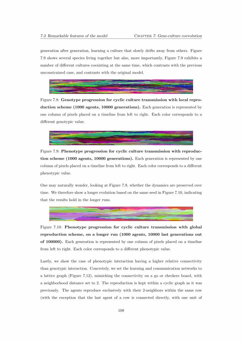
7.3 Remarkable features of the model Chapter 7: Gene-culture coevolution
generation after generation, learning a culture that slowly drifts away from others. Figure
7.9 shows several species living together but also, more importantly, Figure 7.9 exhibits a
number of di↵erent cultures coexisting at the same time, which contrasts with the previous
unconstrained case, and contrasts with the original model.
Figure 7.8: Genotype progression for cyclic culture transmission with local repro-
duction scheme (1000 agents, 10000 generations). Each generation is represented by
one column of pixels placed on a timeline from left to right. Each color corresponds to a
di↵erent genotypic value.
Figure 7.9: Phenotype progression for cyclic culture transmission with reproduc-
tion scheme (1000 agents, 10000 generations). Each generation is represented by one
column of pixels placed on a timeline from left to right. Each color corresponds to a di↵erent
phenotypic value.
One may naturally wonder, looking at Figure 7.9, whether the dynamics are preserved over
time. We therefore show a longer evolution based on the same seed in Figure 7.10, indicating
that the results hold in the longer runs.
Figure 7.10: Phenotype progression for cyclic culture transmission with global
reproduction scheme, on a longer run (1000 agents, 10000 last generations out
of 100000). Each generation is represented by one column of pixels placed on a timeline
from left to right. Each color corresponds to a di↵erent phenotypic value.
Lastly, we show the case of phenotypic interaction having a higher relative connectivity
than genotypic interaction. Concretely, we set the learning and communication networks to
a lattice graph (Figure 7.12), mimicking the connectivity on a go or checkers board, with
a neighborhood distance set to 2. The reproduction is kept within a cyclic graph as it was
previously. The agents reproduce exclusively with their 2-neighbors within the same row
(with the exception that the last agent of a row is connected directly, with one unit of
108
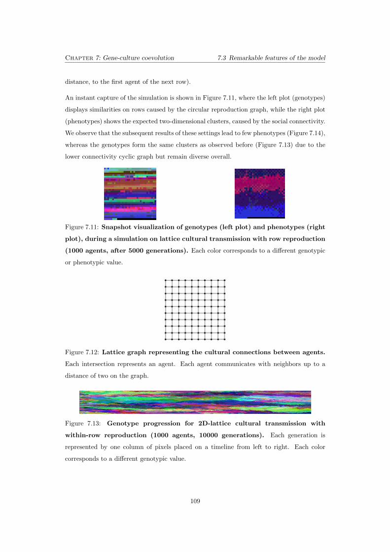
Chapter 7: Gene-culture coevolution 7.3 Remarkable features of the model
distance, to the first agent of the next row).
An instant capture of the simulation is shown in Figure 7.11, where the left plot (genotypes)
displays similarities on rows caused by the circular reproduction graph, while the right plot
(phenotypes) shows the expected two-dimensional clusters, caused by the social connectivity.
We observe that the subsequent results of these settings lead to few phenotypes (Figure 7.14),
whereas the genotypes form the same clusters as observed before (Figure 7.13) due to the
lower connectivity cyclic graph but remain diverse overall.
Figure 7.11: Snapshot visualization of genotypes (left plot) and phenotypes (right
plot), during a simulation on lattice cultural transmission with row reproduction
(1000 agents, after 5000 generations). Each color corresponds to a di↵erent genotypic
or phenotypic value.
Figure 7.12: Lattice graph representing the cultural connections between agents.
Each intersection represents an agent. Each agent communicates with neighbors up to a
distance of two on the graph.
Figure 7.13: Genotype progression for 2D-lattice cultural transmission with
within-row reproduction (1000 agents, 10000 generations). Each generation is
represented by one column of pixels placed on a timeline from left to right. Each color
corresponds to a di↵erent genotypic value.
109
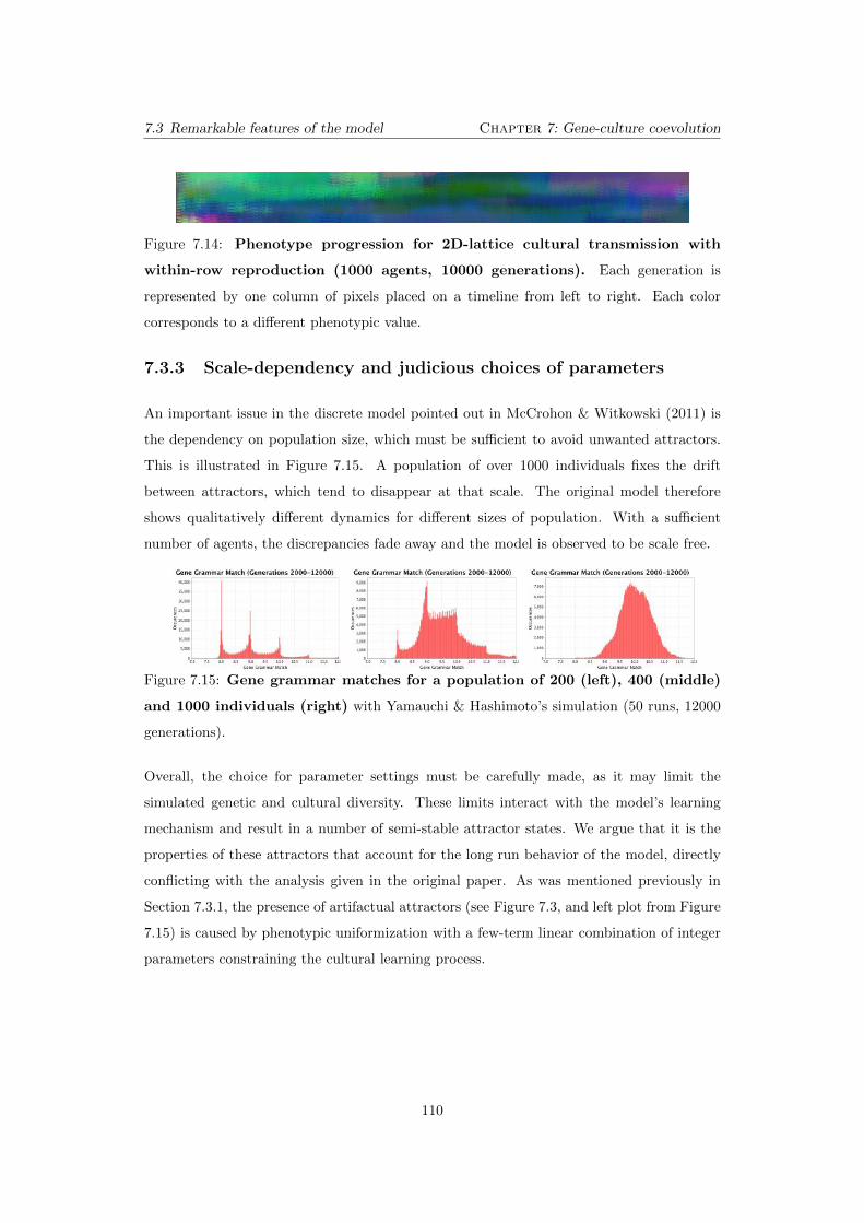
7.3 Remarkable features of the model Chapter 7: Gene-culture coevolution
Figure 7.14: Phenotype progression for 2D-lattice cultural transmission with
within-row reproduction (1000 agents, 10000 generations). Each generation is
represented by one column of pixels placed on a timeline from left to right. Each color
corresponds to a di↵erent phenotypic value.
7.3.3 Scale-dependency and judicious choices of parameters
An important issue in the discrete model pointed out in McCrohon & Witkowski (2011) is
the dependency on population size, which must be su�cient to avoid unwanted attractors.
This is illustrated in Figure 7.15. A population of over 1000 individuals fixes the drift
between attractors, which tend to disappear at that scale. The original model therefore
shows qualitatively di↵erent dynamics for di↵erent sizes of population. With a su�cient
number of agents, the discrepancies fade away and the model is observed to be scale free.
Figure 7.15: Gene grammar matches for a population of 200 (left), 400 (middle)
and 1000 individuals (right) with Yamauchi & Hashimoto’s simulation (50 runs, 12000
generations).
Overall, the choice for parameter settings must be carefully made, as it may limit the
simulated genetic and cultural diversity. These limits interact with the model’s learning
mechanism and result in a number of semi-stable attractor states. We argue that it is the
properties of these attractors that account for the long run behavior of the model, directly
conflicting with the analysis given in the original paper. As was mentioned previously in
Section 7.3.1, the presence of artifactual attractors (see Figure 7.3, and left plot from Figure
7.15) is caused by phenotypic uniformization with a few-term linear combination of integer
parameters constraining the cultural learning process.
110
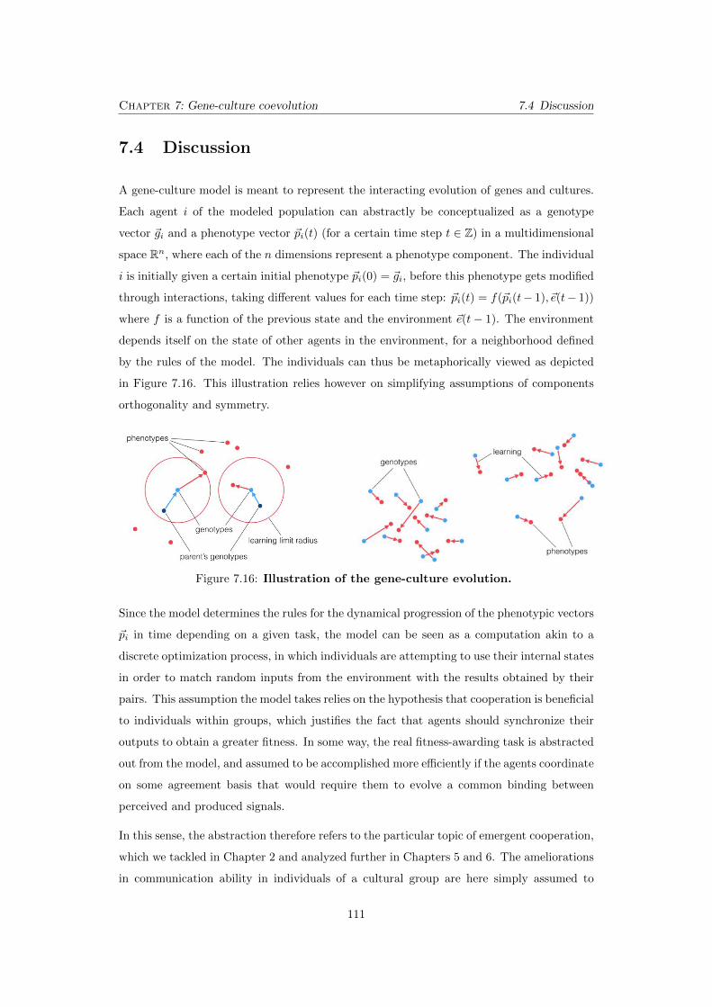
Chapter 7: Gene-culture coevolution 7.4 Discussion
7.4 Discussion
A gene-culture model is meant to represent the interacting evolution of genes and cultures.
Each agent i of the modeled population can abstractly be conceptualized as a genotype
vector ~gi and a phenotype vector ~pi(t) (for a certain time step t 2 Z) in a multidimensional
space Rn, where each of the n dimensions represent a phenotype component. The individual
i is initially given a certain initial phenotype ~pi(0) = ~gi, before this phenotype gets modified
through interactions, taking di↵erent values for each time step: ~pi(t) = f(~pi(t� 1),~e(t� 1))
where f is a function of the previous state and the environment ~e(t� 1). The environment
depends itself on the state of other agents in the environment, for a neighborhood defined
by the rules of the model. The individuals can thus be metaphorically viewed as depicted
in Figure 7.16. This illustration relies however on simplifying assumptions of components
orthogonality and symmetry.
Figure 7.16: Illustration of the gene-culture evolution.
Since the model determines the rules for the dynamical progression of the phenotypic vectors
~pi in time depending on a given task, the model can be seen as a computation akin to a
discrete optimization process, in which individuals are attempting to use their internal states
in order to match random inputs from the environment with the results obtained by their
pairs. This assumption the model takes relies on the hypothesis that cooperation is beneficial
to individuals within groups, which justifies the fact that agents should synchronize their
outputs to obtain a greater fitness. In some way, the real fitness-awarding task is abstracted
out from the model, and assumed to be accomplished more e�ciently if the agents coordinate
on some agreement basis that would require them to evolve a common binding between
perceived and produced signals.
In this sense, the abstraction therefore refers to the particular topic of emergent cooperation,
which we tackled in Chapter 2 and analyzed further in Chapters 5 and 6. The ameliorations
in communication ability in individuals of a cultural group are here simply assumed to
111
7.4 Discussion Chapter 7: Gene-culture coevolution
contribute to the better chances of survival and reproduction of the individual.
These assumptions might sound related to hard behaviorist views of the evolution of com-
munication (Skinner, 1957), where communication is strictly learned through a set of habits
acquired by means of conditioning. This has been criticized as the process would be too
slow, especially for a phenomenon as complicated as language learning (Chomsky, 1959).
However, the behaviorist view suggests that humans could construct linguistic stimuli that
would then acquire control over their behavior, in the same way as external stimuli could
(Skinner, 1969). The idea has recently been extended through the relational frame theory
(Blackledge, 2003), which argues that the building blocks of human language and higher
cognition reside in the ability to create links between concepts.
Nevertheless, as far as the present model is concerned, no real assumption is made in one
direction or the other of the debate. The ABM approach, with the associated declensions
including ANN paradigm and evolutionary algorithm, are compatible with both theories
and may o↵er adequate tools to study them further. Indeed, neural networks do not simply
associate vectors of inputs together, but are also able to perform complex, non-linear classi-
fications and provide responses accordingly, based on the learning algorithms used to train
them, namely evolutionary process and backpropagation.
The reader must be warned on the perhaps classic mode of visualization used in Section 7.3.3
for genetic and phenotypic evolution plots. Although visually clear, they present the obvious
flaw of easily showing clusters in only one dimension. This was especially visible in the case of
latttices, which rapidly show the repetition of lines, which are the artifactual outcome of grid
interactions projected on a single dimension. More advanced methods were used for example
in Chapter 4, taking into account unbounded dimensionality. Also, di↵erent cultures are
simply visualized from weights, which presents a risk of confusion between phenotype and
culture. Furthermore, phenotypes should be graphed as the result of classification tests
on the phenotypes, so that two phenotypes will be similar if they respond in the same way.
Despite these problems, the model is acceptable as a simplification, although must be applied
carefully to evolutionary problems, to avoid the risks of misreading results.
Each individual in Figure 7.16 is shown as a point representing its initial culture, and another
point showing the culture resulting from its learning. The individuals then interact from
neighbor to neighbor, generating the dynamics described above. This is conceptually equiv-
alent to models from oscillator theory, based upon the Ising model (Ising, 1925; Glauber,
1963), or its generalization, the Potts model (Ashkin & Teller, 1943; Potts, 1952). Indeed,
112
Chapter 7: Gene-culture coevolution 7.4 Discussion
the Potts model, by simulating in a very simple way the interaction of spins on a crystalline
lattice, reveals important insights about the behavior of ferromagnets, and demonstrates
basic dynamics of synchrony and phase transitions.
In the light of the theories of phase-coupled oscillators (Strogatz & Mirollo, 1988; Strogatz
et al., 1993), gene-culture models can be seen as a variant allowing to study general interac-
tive systems. The oscillators are found to synchronize in certain configurations, based on the
one hand on their learning patterns from their neighbors’ signals, and on the other hand on
their replication through mutation and selection, which relies on a communicative evaluation
of their fitness. As a result of the creation of this dual interaction between individuals, they
are able to couple and decouple in the same way as oscillators, but with richer dynamics
(Huygens, 1665; Strogatz et al., 1993; Strogatz, 2000, 2003), perhaps as one would expect
from a system involving human behavior.
In the future, the model we presented may o↵er enough generality to study di↵erent phe-
nomena. It may be suited to the study of the emergence of cooperation, while keeping clarity
concerning the ongoing debate on group selection (see Chapter 2). Also, the model is a good
tool to test hypotheses in the study of optimal cultural group sizes in human society.
113
Chapter8Conclusion
This thesis finds its roots from a combination of interests in evolutionary biology, group
dynamics and social behavior. Our goal was to investigate the evolution of collaborative
behaviors of agents based on their communicative interactions. To the best of our knowledge,
a complete explanation of the dynamics and conditions leading to these phenomena has yet
to be established.
Throughout the chapters, we have utilized the agent-based modeling approach to study
the evolution of coordination, as a process occurring among individuals on di↵erent levels of
interaction complexity. Through simulations and analyses, we have shown that coordination
emerges as a product of the cooperation between autonomous agents, given the availability
of a channel for interaction. In every study that was presented, we have demonstrated the
intricate interdependence between coordination, cooperation and communication.
The research methodology, directed at exploring the reasons for the emergence and evolution
of communication, eventually led towards the use of the most simplistic models. In this the-
sis, every chapter posed new questions about the impact of communication on coordination
in increasingly complex systems, from the minimalistic models in Chapters 4 and 5 with
a very simple fitness function, to variable resource environments in Chapter 6, and finally
studying the dynamics of an already established communication system in a gene-culture
coevolution model.
The emergence of communication relies on more than a checklist of conditions that a popu-
lation must fulfill. Rather, it ought to be understood as a historical process of interactions
between generations of individuals embodied in an environment. The population dynamics
must allow the agents to evolve the need to cooperate with each other, so that they would
evolve synergistic relation, which will slowly benefit from growing richer and more complex,
114
Chapter 8: Conclusion 8.1 Recapitulation and contributions
until reaching the level of a fully-fledged communication system.
With these general conclusions in mind, in the following we will summarize the main con-
tributions of this thesis, and evaluate its impact considering past research. We will also
address the shortcomings of our work, and mention possible ameliorations in future work.
The raison d’etre of this chapter is to clarify the claims made earlier in this thesis, to ensure
the reader possesses all the elements to accurately grasp the nature and significance of the
results we present. Finally, we also want to o↵er a larger picture, placing the presented
research in a general context.
8.1 Recapitulation and contributions
The coordination between agents, a concept defined in Chapter 2, is surely the most recur-
rent of the themes of this thesis, as it holds a central role in each of the presented works.
Every presented study indeed shows a new result that completes the large picture on the
evolution of stigmergic behavior, self-reinforcing activities among groups and exploring the
establishment of increasingly complex coordination patterns. Along the chapters of the thesis
are explored, ordered by complexity, increasingly intricate mechanisms, starting from basic
signaling interactions and simple synchronizations patterns to finish with more convoluted
kinds of coordinations.
In Chapter 4, we demonstrated the emergence of swarming behavior based on signaling.
A minimalistic simulation of autonomous agents, uniquely exchanging local signals in a
three-dimensional environment, become able to form temporary leader-follower relations to
dynamically flock together.
Another type of swarming is then shown in Chapter 5, where we simulate a dynamical
version of the spatial Prisoner’s Dilemma. The cooperating agents are found to evolve a
clustering behavior corresponding to a degenerated version of the dynamics produced in
Chapter 4. This spatial coordination is especially interesting for it is explicitly connected
with the cooperative behavior. The clustering is also found to be bistable, and cooperators
are moving quickly inside the cluster to avoid cheating predators. A moving cluster of
cooperators is more stable against defector invasions, bringing a soft bistability to the system,
which may easily switch between cooperative to defective state.
Next, Chapter 6 puts coordination to the test with simulations in unpredictable environ-
115
8.1 Recapitulation and contributions Chapter 8: Conclusion
ments, showing evolutionary stable solutions involving coordination. Individuals are shown
to either evolve the ability to synchronize based on each other’s signals, or evolve other adap-
tive behaviors to overcome the variable resource conditions. The coordination in this chapter
takes the form of a temporal synchronization, able to synchronize the group’s motion around
a ring map, to synchronize the right timing to solve the migration timing problem, or indi-
vidual specific resource-saving strategies, which synchronize simply with the environments
in case no other information channel is open apart from food scarcity.
Up to this point of the thesis, all the studied adaptive behaviors, with the exception of the
hoarding behavior in Section 6.4, are coordinations based on signaling. The agents eventually
evolve a signaling behavior such that it can be used by the group to coordinate together
in an e�cient behavior, giving the agents greater fitness, and thus chances of survival and
reproduction.
Finally, in Chapter 7 coordination is observed both within genetic and phenotypic timelines
in a coevolution model. The individuals’ genotypes are able to climb fitness gradients by
themselves, but may be helped by the appendage of cultural learning. Learned behaviors
may then take over unlearned ones (shielding), and vice versa (Baldwin e↵ect, cf. Section
7.1), creating a di↵erent type of information transfer, not only among individuals of the
population this time, but from one evolutionary system to another. Coordination is thus
dual, with the formation of clusters in the cultural or genetic space, but also with the creation
of dynamical information flows between genetic and cultural lineages.
The synergistic coordination among agents originates from cooperation, which constitutes
a second recurrent theme in this thesis, is based upon the interactions involved in the
coordination dynamics that were just mentioned. The selection of cooperation is in essence
a delicate topic in the study of behavioral and evolutionary ecology, in part because of its
debated theories of group selection and the origins of altruism, as evoked in Chapter 2.
Nevertheless, it is compulsory to discuss its mechanisms, as they have a direct impact on
the creation of positive feedbacks on the evolution of coordination.
In particular, Chapter 5 details the possible impact of cooperative behavior on coordination
of behaviors, focusing on the dynamics of spatial groups. Chapters 4 and 6 also tackle the
subject of cooperation, as the behaviors are evolved based on the help of kin-selection in
relatively small populations. Lastly, Chapter 7 takes cooperation as granted, and based on
this assumption, examines further certain high-level dynamics of gene-culture coevolution.
The evolution of a communicative system is the third of the main themes treated in this
116
Chapter 8: Conclusion 8.2 Limitations
thesis, although its importance is as fundamental as the previous ones, as it is intimately
related to them. Indeed, communication is commonly considered to be a complex adaptation
facilitating cooperative behavior (Richerson & Boyd, 2010). As such, it is directly based on
coordination and cooperation.
The way communicative behavior was treated in the thesis follows once more a progression of
less to more complex level of communication. Chapters 4 and 5 have basic signaling emerge
from local interactions, Chapter 6 takes the signaling system a little further by assigning
meaning values in certain cases (see Section 6.2), and finally in Chapter 7 (and partly Section
6.3) communication is considered in its accomplished form, with a cultural tradition passed
on via social learning.
Given our approach is borrowed from evolutionary robotics (Section 3.1), evolutionary e↵ects
constitute a very important topic in every chapter of the thesis. In particular, Sections 6.3
and 7.3 show the e↵ects of cultural learning by mimicry, that is by partly matching the
learner’s culture to another agents’. The results show that this learning leads to rapid
fitness increases over the whole population, but also brings a higher risk of fitness drops.
Those are found to be caused by occasional mimicking of ine�cient phenotypes in Chapter
6. In the case of the gene-culture model introduced in Chapter 7, the drops are not caused
directly by an overfitting issue between individuals, but by the interaction between gene
and culture. That interaction is found to create a transfer of fitness-fulfilling load back and
forth from the genotypes to the culture and vice-versa.
8.2 Limitations
The work presented in this thesis contributes to the literature in a number of fields such as
artificial life modeling, swarm dynamics and social behavior. Scientific research is almost
never a complete success story, and numerous parts in this thesis could have been approached
in a di↵erent way than they were.
Firstly, the goal was the investigation of collaborative behaviors based on communication, in
an evolutionary perspective. In nature, the stigmergic phenomena, in which mechanisms of
coordination between agents are observed, based on a certain interaction they have among
them. The connection between their global coordination and their local interaction repre-
sents the subject of this thesis. A complete theory of the evolution of coordination and
communication should explain and justify all the initial ingredients and all the subsequent
117
8.2 Limitations Chapter 8: Conclusion
dynamics necessary to the emergence of the observed phenomena. Although this thesis
brings the elements mentioned above to answer that question, it does not yet allow for a
complete explanation of the emergence of coordination based on communication in the sense
of a complete theory. For that reason, our research has to be understood as an attempt to
improve existing frameworks of theories in the field.
Secondly, a confusion may occur in the reader’s mind, as for the distinction made between
coordination and cooperation, underlined in Chapters 1 and 2. The definition given in
Chapter 2 classifies coordination as the behavioral organization between agents which en-
ables them to fulfill a desired goal. Cooperation, on the other hand, is defined as the action
for a common or mutual benefit, which is typically defined as an adaptation to increase the
reproductive success of other agents rather than itself. As a matter of fact, coordination,
as it was observed in the di↵erent experiments of this thesis, always arose from the coop-
eration between agents, i.e. their collaboration to fullfill common goals. This is due, in
our setups, to the emergence of reciprocal selection (Trivers, 1971; Axelrod, 1984) and kin
selection (Smith, 1964; Hamilton, 1964), which lead the agents in the simulated populations
to evolve altruistic behaviors, which is the coordinated behavior of interest. That behavior
is signal-based swarming in Chapters 4 and 5, and signal-based synchronization in Chapter
6.
Thirdly, a minor source of confusion may arise from the diverse formulations of the agent-
based modeling we refer to in the literature, as the field of study continually crosses borders
between di↵erent areas, from nonlinear systems to behavioral biology. For instance, the mod-
eled actors are often referred to as agents, creatures, oscillators and phenotypes, depending
on the context of the discussion. In this thesis, we have put special e↵ort into making the
vocabulary uniform accross the chapters, but certain cases remained problematic where the
choice of terminology was relevant to the discussion. This type of hyperonymy, although
possibly confusing to the neophyte, is probably not new to the researcher working at the
intersection of di↵erent fields of research, which has become more and more frequent in
modern science. The reader may refer to the glossary at the end of this thesis, or to the
literature review and explanations of this thesis, in Chapters 2 and 3.
Other limitations must be considered, that are inherent to the very choice of our method-
ology, using agent-based modeling (ABM). Indeed, such models come with a certain set of
limitations, which can be dangerous if not taken seriously (Castle & Crooks, 2006).
Firstly, the design of the model always constrains its level of description (Couclelis, 2002).
118
Chapter 8: Conclusion 8.2 Limitations
This problem must not be stigmatized in ABM approaches only, as simplifying assumptions
are common too in classical approaches. However, the coordinated patterns we observed
in every chapter required additionally careful analysis. For example, in Chapter 4, the
swarming behavior could have been produced by simple local reproduction, which would
have produced clusters of agents without any need for signaling. Another example is the
avoidance of unwanted, artifactual attractors in Chapter 7.
Secondly, the results must be interpreted appropriately, as the accuracy and completeness
depends on the model’s definition. Multiple runs must always be performed, with a system-
atical varitation of the initial parameters to assess the robustness of results (Axtell, 2000).
This can be an issue in the case that high computational requirements are needed, typically
when the size of the population grows higher, which is a limitation for every one of the stud-
ies presented in this thesis. In particular the evolution of swarming in Chapter 4 required
many runs with a large number of agents, that were modeled by computing-costly neural
networks.
Thirdly, in spite of the biological context in our studies, no empirical study was o↵ered. The
experiments presented in this thesis, although inspired by biological phenomena and given
similar designs, rely exclusively on abstract modeling of natural phenomena. Consequently,
the obtained results will require a distinct set of studies to establish the link with the
real world phenomena. However, we must underline that every model’s purpose was not
to give an accurate quantitative forecast of real biological individuals. But rather, ABM
is used as a tool to explore the intricacies of complex behaviors found in nature, because
of its abstraction (making it verifiable), modularity (each agent is modeled individually),
stochasticity (allowing to assess the probability of emergence by running the simulation
many times) and ability to model emergent properties (local properties translating into
global results).
Of course, if this thesis had to be done all over again, it could be improved on numerous
points, and our methodology can be improved in every way mentioned above. Nevertheless,
in spite of these imperfections, we have brought awareness on concepts, modeling approaches
and specific techniques with a valuable contribution to the field of study.
119
8.3 Future directions Chapter 8: Conclusion
8.3 Future directions
Although the studies presented in this thesis are considered to have reached a stage of
completion, it is our hope at this point that the reader will be left with the feeling that the
research could be expanded much more along similar lines of research. We will conclude with
some ending considerations on the completed work and a few thoughts for future research.
In this thesis, we introduced the problems of the evolution of coordination and communica-
tion. We successfully demonstrated the emergence of spatial coordination from the exchange
of signals between agents in a resource foraging task. Cooperation has been shown to emerge
and create niches through the establishment of signaling. Communication itself has been
shown to emerge in an environment changing with time where cooperation allows individ-
uals to save energy. We have presented multiple models demonstrating the evolution of
communication in populations of agents.
The models we introduced present a significance for both scientific and technological inter-
ests. On the one hand, the ecological studies contribute in themselves to shed light on the
evolution of coordination and communication. On the other hand, a better understanding
of the fundamental principles of collective behavior may also help to design robust control
structures for multi-agents systems, ubiquitous computing devices and swarm computation.
This thesis is intended as a first step towards the comprehension of the evolution of coordi-
nation and communication, by using the methodology of artificial neural networks, shaped
by artificial evolution to control autonomous agents. The long-term goal is to extend our
models for a full understanding of the necessary and su�cient conditions for the emergence
of cooperation between agents, and the dynamics through which they evolve a language.
In the future, in order to achieve these longer term goals, we can easily imagine extensions
for the models we created. Here, we would like to speculate on possible directions in which
to take the next step.
It would be interesting to study, for instance, the impact of the groups’ size on the observed
dynamics. By achieving a critical size, systems may give rise to qualitative changes, allowing
to develop crowd intelligence. The approach introduced in Chapter 4 seems particularly
fruitful to extend along these lines. Also, the approach from Chapter 6 can be appropriate
to study the ability of larger size groups to overcome the small errors and fluctuations arising
in an unpredictable environments, leading them to climb more e�ciently the gradients of
information of their environment, in order to survive better than single individuals would.
120
Chapter 8: Conclusion 8.3 Future directions
A robust theory of criticality in biological systems could benefit from this approach, helping
to characterize the emergence of critical points and phase transitions in real swarms (Mora
& Bialek, 2011; Attanasi et al., 2014b,a).
We would also like to study the influence of sexual dimorphism on the interactions occurring
between agents, in particular the evolution of cooperation in groups. The idea is that sexual
selection could shape groups’ cooperation and conformity to norms (Gintis et al., 2001;
Krebs & Janicki, 2004). The latter one was part of the modeling hypotheses we made in
Chapter 7.
Lastly, we would like to propose an application of our models to the understanding of the
emergence of a “herd morality” (Nietzsche, 1967, 2011), a sense of morality inherent to
cultures. Modeling crowd dynamics may provide insights on the evolution of cooperation
and morality.
121

8.3 Future directions Chapter 8: Conclusion
122
Glossary
ABM Agent-Based Modeling 80
adaptive behavior In behavioral ecology an adaptive behavior is a behavior which contributes
directly or indirectly to an individual’s survival or reproductive success and is thus subject
to the forces of natural selection. 1, 9
ANN An ANN, or artificial neural network, is a computational model inspired by biological neural
networks and are used to estimate or approximate functions that can depend on a large
number of inputs and are generally unknown. 38, 104
coevolution In evolutionary biology, coevolution refers to the changes to which a biological species
is subject, which are triggered by the changes in another species. That is, coevolution refers
to the phenomenon of two species’ genetic compositions reciprocally a↵ecting each other’s
evolution. 8
communication Communication is the interaction between agents that enables them to trans-
fer information to each other across space and time, creating the possibility for complex
mechanisms such as language. 2–4
cooperation In evolutionary game theory, cooperation is the adaptation in groups of agents that
makes them work together for mutual benefits, as opposed to uniquely competitive or selfish
benefit. An agent is considered to be cooperating if it sacrifices some of its own reproductive
potential to help increasing other agents’ chances of reproductive success. 2–4, 14, 15
coordination In the context of adaptive behavior, coordination is the organization of di↵erent
individuals of a population, or elements of a complex entity, enabling them to work together
e↵ectively. 1–4, 15
DNA DNA, or deoxyribonucleic acid, is a molecule that encodes the genetic instructions used in
the development and functioning of living organisms. They contain the hereditary material
in every species, what makes them unique. 9, 124
123
Glossary Glossary
embodied An embodied agent is an agent which is given a body in a material or simulated
world, which will largely determine the nature of its cognitive abilities (Brooks, 1992). The
terminology comes from the theory of embodied cognition, originating from Kant & Jaki
(1981). 2, 27
epigenetics In biology, epigenetics is the study of cellular and physiological traits that are not
caused by changes in the DNA sequence; Epigenetics describes the study of stable, long-term
alterations in the transcriptional potential of a cell. Some of those alterations are heritable.
11
evolution Evolution is the process by which di↵erent kinds of living organisms gradually develop
and diversified from earlier forms during the history of the earth. 1, 2
gene The term gene refers to the cause of an inheritable phenotype characteristic (e.g. skin color
or number of legs). 9
go The game of go, also known as igo, baduk or weiqi, is a board game involving two players
playing black and white stones on the vacant intersections of a board with a 19x19 grid of
lines. 108
heritable A characteristic or trait in an individual is said to be heritable, if it is transmissible
from parent to o↵spring. Heritability is therefore considered to be the proportion of observed
di↵erences on a trait among individuals of a population that are due to genetic di↵erences.
9
locus In genetics, a locus refers to a specific location on a chromosome, that can correspond to a
gene or DNA sequence. 17
Prisoner’s Dilemma Canonical example of a non-zero-sum game, where two players can choose
between two moves, either “cooperate” or “defect”. The idea is that each player gains when
both cooperate, but if only one of them cooperates, the one who defects gains more. If
both defect, both lose (or gain less) although not as much as the cheated cooperator whose
cooperation is not returned. 64
RNA RNA, or ribonucleic acid, is a polymeric molecule implicated in the coding, decoding, regu-
lation, and expression of genes. 13
shielding Shielding is the e↵ect of learned behavior replacing unlearned behavior. Shielding is
said to “mask” natural selection. It is often considered as the opposite of the Baldwin e↵ect,
in the sense that a species that learns a feature, does not need to evolve it. 102, 106, 116
signal A signal is defined as any act or structure which alters the behavior of other organisms,
which evolved because of that e↵ect, and which is e↵ective because the receiver’s response
has also evolved. 125
124
Glossary Glossary
signaling Use of signals between agents. 2
stigmergy Stigmergy is a mechanism of indirect coordination between agents or actions. The
principle is that the trace left in the environment by an action stimulates the performance of
a next action, by the same or a di↵erent agent. In that way, subsequent actions tend to rein-
force and build on each other, leading to the spontaneous emergence of coherent, apparently
systematic activity. Stigmergy is a form of self-organization. It produces complex, seemingly
intelligent structures, without need for any planning, control, or even direct communication
between the agents. As such it supports e�cient collaboration between extremely simple
agents, who lack any memory, intelligence or even individual awareness of each other. 2, 15
theory of mind The ability to attribute mental states (e.g. beliefs, intentions or desires) to oneself
and others and to understand that others have beliefs, desires, and intentions that are di↵erent
from one’s own. 23
125
References
C Aktipis. 2004. Know when to walk away: contingent movement and the evolution of cooperation.
Journal of Theoretical Biology, 231, 249–260.
C Aktipis. 2011. Is cooperation viable in mobile organisms? simple walk away rule favors the
evolution of cooperation in groups. Evolution and Human Behavior, 32, 263–276.
C Yu Albert and Daniel Margoliash. 1996. Temporal hierarchical control of singing in birds. Science,
273, 1871–1875.
Malte Andersson and John Krebs. 1978. On the evolution of hoarding behaviour. Animal Behaviour,
26, 707–711.
Alex Arenas, Albert Dıaz-Guilera and Conrad J Perez-Vicente. 2006. Synchronization reveals
topological scales in complex networks. Physical review letters, 96, 114102.
T. Arita and Y. Koyama. 1998. Evolution of linguistic diversity in a simple communication system.
Artificial Life, 4(4), 109–124.
Julius Ashkin and Edward Teller. 1943. Statistics of two-dimensional lattices with four components.
Physical Review, 64, 178.
Alessandro Attanasi, Andrea Cavagna, Lorenzo Del Castello, Irene Giardina, Stefania Melillo,
Leonardo Parisi, Oliver Pohl, Bruno Rossaro, Edward Shen, Edmondo Silvestri and Massim-
iliano Viale. 07 2014a. Collective behaviour without collective order in wild swarms of midges.
PLoS Comput Biol, 10, e1003697. URL http://dx.doi.org/10.1371%2Fjournal.pcbi.1003697.
(doi:10.1371/journal.pcbi.1003697)
Alessandro Attanasi, Andrea Cavagna, Lorenzo Del Castello, Irene Giardina, Stefania Melillo,
Leonardo Parisi, Oliver Pohl, Bruno Rossaro, Edward Shen, Edmondo Silvestri and Massimiliano
Viale. Dec 2014b. Finite-size scaling as a way to probe near-criticality in natural swarms. Phys.
Rev. Lett., 113, 238102. URL http://link.aps.org/doi/10.1103/PhysRevLett.113.238102.
(doi:10.1103/PhysRevLett.113.238102)
126
REFERENCES REFERENCES
Athula B Attygalle and E David Morgan. 1985. Ant trail pheromones. Advances in Insect Physiology,
18, 1–30.
R. Axelrod. The Evolution of Cooperation. Basic Books, New York, USA, 1984.
Robert Axelrod and William D Hamilton. 1981. The evolution of cooperation. Science, 211,
1390–1396.
Robert Axtell. 2000. Why agents?: on the varied motivations for agent computing in the social
sciences.
Andrew C Baker, Craig J Starger, Tim R McClanahan and Peter W Glynn. 2004. Coral reefs:
corals’ adaptive response to climate change. Nature, 430, 741–741.
James E Baker. Reducing bias and ine�ciency in the selection algorithm. In Proceedings of the
Second International Conference on Genetic Algorithms and their Application, pages 14–21. Hills-
dale, New Jersey: L. Erlbaum Associates, 1987.
J. Mark Baldwin. 1896. A new factor in evolution. The American Naturalist, 30, 441–451.
M. Ballerini, N. Cabibbo, R. Candelier, A. Cavagna, E. Cisbani, I. Giardina, V. Lecomte,
A. Orlandi, G. Parisi, A. Procaccini, M. Viale and V. Zdravkovic. 2008. Interaction rul-
ing animal collective behavior depends on topological rather than metric distance: Evidence
from a field study. Proceedings of the National Academy of Sciences, 105, 1232–1237. URL
http://www.pnas.org/content/105/4/1232.abstract. (doi:10.1073/pnas.0711437105)
AV Bardin and MY Markovets. 1991. Rate of plundering of reserves by tits: experimental investi-
gations. Soviet J Ecol, 61, 322–336.
Simon Baron-Cohen, Howard A Ring, Sally Wheelwright, Edward T Bullmore, Mick J Brammer,
Andrew Simmons and Steve CR Williams. 1999. Social intelligence in the normal and autistic
brain: an fmri study. European Journal of Neuroscience, 11, 1891–1898.
M. Bartlett and D. Kazakov. 2005. The origins of syntax: from navigation to language. Connection
Science, 17(1), 271–288.
S. Bauer, B. Nolet, J. Giske, J. Chapman, S. Akesson, A. Hedenstrom and J. Fryxell. Cues and
decision rules in animal migration. In J. Fryxell E. Milner-Gulland and A. Sinclair, editors,
Animal Migration: A Synthesis, pages 69–87. Oxford University Press, Oxford, UK, 2011.
Mark A Bedau, John S McCaskill, Norman H Packard, Steen Rasmussen, Chris Adami, David G
Green, Takashi Ikegami, Kunihiko Kaneko and Thomas S Ray. 2000. Open problems in artificial
life. Artificial life, 6, 363–376.
Randall D Beer. 1995. A dynamical systems perspective on agent-environment interaction. Artificial
intelligence, 72, 173–215.
127
REFERENCES REFERENCES
R Alexander Bentley, Matthew W Hahn and Stephen J Shennan. 2004. Random drift and culture
change. Proceedings of the Royal Society of London. Series B: Biological Sciences, 271, 1443–
1450.
Theodore C Bergstrom. 2002. Evolution of social behavior: individual and group selection. Journal
of Economic Perspectives, pages 67–88.
John T Blackledge. 2003. An introduction to relational frame theory: Basics and applications. The
Behavior Analyst Today, 3, 421–433.
Vincent Blondel, Julien M Hendrickx, Alex Olshevsky and J Tsitsiklis. Convergence in multiagent
coordination, consensus, and flocking. In IEEE Conference on Decision and Control, volume 44,
page 2996. IEEE; 1998, 2005.
Eric Bonabeau, Marco Dorigo and Guy Theraulaz. Swarm intelligence: from natural to artificial
systems. Number 1. Oxford university press, 1999.
Eric Bonabeau, Marco Dorigo and Guy Theraulaz. 2000. Inspiration for optimization from social
insect behaviour. Nature, 406, 39–42.
Eric Bonabeau, Guy Theraulaz, Jean-Louls Deneubourg, Serge Aron and Scott Camazine. 1997.
Self-organization in social insects. Trends in Ecology & Evolution, 12, 188–193.
Peter J Bowler. Evolution: the history of an idea. Univ of California Press, 1989.
Robert Boyd and Peter J Richerson. 1992. Punishment allows the evolution of cooperation (or
anything else) in sizable groups. Ethology and sociobiology, 13, 171–195.
Hans J Bremermann. 1962. Optimization through evolution and recombination. Self-organizing
systems, pages 93–106.
Ted Briscoe. Grammatical acquisition: Coevolution of language and the language acquisition device.
In In Proceedings of the Diachronic Generative Syntax. Oxford University Press, 1998.
Anders Brodin and Jan Ekman. 1994. Benefits of food hoarding. Nature.
Rodney A Brooks. 1991. Intelligence without representation. Artificial intelligence, 47, 139–159.
Rodney A Brooks. Artifical life and real robots. In Toward a practice of autonomous systems: Proc.
of the 1st Europ. Conf. on Artificial Life, page 3, 1992.
Jerome S Bruner. 1981. Intention in the structure of action and interaction. Advances in infancy
research.
Elena O Budrene, Howard C Berg et al. 1991. Complex patterns formed by motile cells of escherichia
coli. Nature, 349, 630–633.
128
REFERENCES REFERENCES
Richard W Byrne and Andrew Whiten. 1989. Machiavellian intelligence: Social expertise and the
evolution of intellect in monkeys, apes, and humans (oxford science.
A. Cangelosi. 2001. The emergence of a language in an evolving population of neural networks.
IEEE Transactions in Evolution Computation, 5(1), 93–101.
Christian JE Castle and Andrew T Crooks. 2006. Principles and concepts of agent-based modelling
for developing geospatial simulations.
Nick Chater, Florencia Reali and Morten Christiansen. Jan 27 2009. Restrictions on biological
adaptation in language evolution. PNAS, 106, 1015–1020. URL http://www.isrl.uiuc.edu/
~
amag/langev/paper/chater09restrictionsPNAS.html. (doi:10.1073/pnas.0807191106)
Zhuo Chen, Jianxi Gao, Yunze Cai and Xiaoming Xu. 2011. Evolution of cooperation among mobile
agents. Physica A: Statistical Mechanics and its Applications, 390, 1615–1622.
Raymond Chiong and Michael Kirley. 2012. Random mobility and the evolution of cooperation
in spatial n-player iterated prisoner’s dilemma games. Physica A: Statistical Mechanics and its
Applications, 391, 3915–3923.
Noam Chomsky. 1959. A review of bf skinner’s verbal behavior. Language, 35, 26–58.
Noam Chomsky. The minimalist program, volume 28. Cambridge Univ Press, 1995.
Noam Chomsky. 2005. Three factors in language design. Linguistic inquiry, 36, 1–22.
Chun Wei Choo. The knowing organization: How organizations use information to construct mean-
ing, create knowledge, and make decisions, volume 256. Oxford university press New York, 1998.
Morten H Christiansen and Simon Kirby. 2003. Language evolution: Consensus and controversies.
Trends in cognitive sciences, 7, 300–307.
Jongsik Chun, Jae-Hak Lee, Yoonyoung Jung, Myungjin Kim, Seil Kim, Byung Kwon Kim and
Young-Woon Lim. 2007. Eztaxon: a web-based tool for the identification of prokaryotes based
on 16s ribosomal rna gene sequences. International Journal of Systematic and Evolutionary
Microbiology, 57, 2259–2261.
Michael F Clarke and Donald L Kramer. 1994. The placement, recovery, and loss of scatter hoards
by eastern chipmunks, tamias striatus. Behavioral Ecology, 5, 353–361.
Tim Clutton-Brock. 2002. Breeding together: kin selection and mutualism in cooperative verte-
brates. Science, 296, 69–72.
John Coleman and B Keith. 2006. Design features of language. Brown (ed.), pages 471–5.
Kevin J Connolly and Margaret Martlew. Psychologically speaking: A book of quotations. Blackwell
Publishing, 1999.
129
REFERENCES REFERENCES
John Conway. 1970. The game of life. Scientific American, 223, 4.
Sandra Cortijo, Rene Wardenaar, Maria Colome-Tatche, Arthur Gilly, Mathilde Etcheverry, Karine
Labadie, Erwann Caillieux, Jean-Marc Aury, Patrick Wincker, Francois Roudier et al. 2014.
Mapping the epigenetic basis of complex traits. science, 343, 1145–1148.
Helen Couclelis. 2002. Modeling frameworks, paradigms, and approaches. Geographic Information
Systems and Environmental Modelling, Prentice Hall, London.
Cyril Courtin. 2000. The impact of sign language on the cognitive development of deaf children
the case of theories of mind. Journal of Deaf Studies and Deaf Education, 5, 266–276.
Iain D Couzin. 2009. Collective cognition in animal groups. Trends in cognitive sciences, 13, 36–43.
Iain D Couzin, Jens Krause, Richard James, Graeme D Ruxton and Nigel R Franks. 2002. Collective
memory and spatial sorting in animal groups. Journal of theoretical biology, 218, 1–11.
Felipe Cucker and Cristian Huepe. 2008. Flocking with informed agents. Mathematics in Action,
1, 1–25.
Andras Czirok, Albert-Laszlo Barabasi and Tamas Vicsek. 1997. Collective motion of self-propelled
particles: Kinetic phase transition in one dimension. arXiv preprint cond-mat/9712154.
Charles Darwin. The descent of man. Digireads. com Publishing, 2004 edition, 1871.
Charles Darwin and Alfred Wallace. 1858. On the tendency of species to form varieties; and on the
perpetuation of varieties and species by natural means of selection. Journal of the proceedings of
the Linnean Society of London. Zoology, 3, 45–62.
Richard Dawkins. 1989. The selfish gene. 1976. revised edn. Oxford.
Richard Dawkins. The ancestor’s tale: a pilgrimage to the dawn of evolution. Houghton Mi✏in
Harcourt, 2005.
Richard Dawkins. The selfish gene. Number 199. Oxford university press, 2006.
Richard Dawkins and John R Krebs. 1978. Animal signals: information or manipulation. Be-
havioural ecology: An evolutionary approach, 2, 282–309.
B. De Boer. 1999. Evolution and self-organisation in vowel systems. Evolution of Communication,
3(1), 79–103.
Kevin De Queiroz. 2005. Ernst mayr and the modern concept of species. Proceedings of the National
Academy of Sciences, 102, 6600–6607.
Terrence W. Deacon. The Symbolic Species: The Co-evolution of Language and the Brain. W.W.
Norton, 1997. URL http://www.isrl.uiuc.edu/
~
amag/langev/paper/deacon97theSymbolic.
html.
130
REFERENCES REFERENCES
Terrence W Deacon. 2003a. The hierarchic logic of emergence: Untangling the interdependence of
evolution and self-organization. Evolution and learning: The Baldwin e↵ect reconsidered, pages
273–308.
Terrence W. Deacon. Multilevel selection in a complex adaptive system: The problem of language
origins. [References]. In A,, Division, Department and Anonymous, editors, Evolution and Learn-
ing: The Baldwin E↵ect Reconsidered. Life and mind, pages 81–106. The MIT Press, 2003b. ISBN
0-262-23229-4 (hardcover).
Marc Peter Deisenroth, Gerhard Neumann and Jan Peters. 2013. A survey on policy search for
robotics. Foundations and Trends in Robotics, 2, 1–142.
Kristin Denham and Anne Lobeck. Linguistics for everyone: An introduction. Cengage Learning,
2012.
Daniel C Dennett. 2003. The baldwin e↵ect: A crane, not a skyhook. Evolution and learning: The
Baldwin e↵ect reconsidered, pages 60–79.
John Dewey. Experience and nature, volume 1. Courier Dover Publications, 1958.
Ezequiel A Di Paolo. 1997. An investigation into the evolution of communication. Adaptive
Behavior, 6, 285–324.
Ezequiel Alejandro Di Paolo. On the evolutionary and behavioral dynamics of social coordination:
Models and theoretical aspects. University of Sussex, 1999.
Karl C Diller and Rebecca L Cann. 2009. Evidence against a genetic-based revolution in language
50,000 years ago. The cradle of language, 12, 135.
Theodosius Dobzhansky and Theodosius Grigorievich Dobzhansky. Genetics and the Origin of
Species. Number 11. Columbia University Press, 1937.
Theodosius Dobzhansky et al. Genetics of the evolutionary process, volume 139. Columbia Univer-
sity Press New York, 1970.
Calaway H Dodson. 1975. Coevolution of orchids and bees. Coevolution of animals and plants, 91,
99.
Fred C Dyer and Je↵rey A Dickinson. 1996. Sun-compass learning in insects: Representation in a
simple mind. Current Directions in Psychological Science, pages 67–72.
Russ C Eberhart and James Kennedy. A new optimizer using particle swarm theory. In Proceedings
of the sixth international symposium on micro machine and human science, volume 1, pages
39–43. New York, NY, 1995.
Gerald M Edelman. 2006. The embodiment of mind. Daedalus, 135, 23–32.
131
REFERENCES REFERENCES
S. Edwards. The Chaos of Forced Migration: A Means of Modeling Complexity for Humanitarian
Ends. Oxford University Press, Oxford, United Kingdom, 2009.
A. Eiben and J. Smith. Introduction to Evolutionary Computing. Springer-Verlag, Berlin, Germany,
2003.
Jan Ekman, Anders Brodin, Anders Bylin and Bohdan Sklepkovych. 1996. Selfish long-term benefits
of hoarding in the siberian jay. Behavioral Ecology, 7, 140–144.
Je↵rey L Elman. 1990. Finding structure in time. Cognitive science, 14, 179–211.
John A Endler. Natural selection in the wild. Number 21. Princeton University Press, 1986.
DanielL Everett. 2005. Cultural constraints on grammar and cognition in piraha. Current anthro-
pology, 46, 621–646.
Michael A Ewert and Craig E Nelson. 1991. Sex determination in turtles: diverse patterns and
some possible adaptive values. Copeia, pages 50–69.
Eva M Fernandez and Helen Smith Cairns. Fundamentals of psycholinguistics. John Wiley & Sons,
2010.
RA Fisher. The theory of natural selection, 1930.
Ronald Aylmer Fisher. The genetical theory of natural selection. , 1958.
W Tecumseh Fitch. 2004. Kin selection and ‘mother tongues’: a neglected component in language
evolution. Evolution of communication systems: A comparative approach, pages 275–296.
W Tecumseh Fitch. 2011. Unity and diversity in human language. Philosophical Transactions of
the Royal Society B: Biological Sciences, 366, 376–388.
D. Floreano, P. Durr and C. Mattiussi. 2008. Neuroevolution: from architectures to learning.
Evolutionary Intelligence, 1, 47–62.
Dario Floreano, Sara Mitri, Stephane Magnenat and Laurent Keller. 2007. Evolutionary conditions
for the emergence of communication in robots. Current biology, 17, 514–519.
AS Fraser. 1960. Simulation of genetic systems by automatic digital computers vii. e↵ects of repro-
ductive ra’l’e, and intensity of selection, on genetic structure. Australian Journal of Biological
Sciences, 13, 344–350.
Andy Gardner, Ashleigh S Gri�n and Stuart A West. 2009. Theory of cooperation. eLS.
Andy Gardner and Stuart A West. 2010. Greenbeards. Evolution, 64, 25–38.
R Allen Gardner and Beatrice T Gardner. 1969. Teaching sign language to a chimpanzee. Science,
165, 664–672.
132
REFERENCES REFERENCES
R Allen Gardner and Beatrice T Gardner. 1975. Early signs of language in child and chimpanzee.
Science, 187, 752–753.
Anatolij Gelimson, Jonas Cremer and Erwin Frey. 2013. Mobility, fitness collection, and the
breakdown of cooperation. Physical Review E, 87, 042711.
Herbert Gintis. Game theory evolving: A problem-centered introduction to modeling strategic inter-
action. Princeton University Press, 2009.
Herbert Gintis, Eric Alden Smith and Samuel Bowles. 2001. Costly signaling and cooperation.
Journal of theoretical biology, 213, 103–119.
Roy J Glauber. 1963. Time-dependent statistics of the ising model. Journal of mathematical
physics, 4, 294–307.
Jesus Gomez-Gardenes, Yamir Moreno and Alex Arenas. 2007. Paths to synchronization on complex
networks. Physical review letters, 98, 034101.
Jane Goodall. 1986. The chimpanzees of gombe: Patterns of behavior.
Jonathan Grainger, Stephane Dufau, Marie Montant, Johannes C Ziegler and Joel Fagot. 2012.
Orthographic processing in baboons (papio papio). Science, 336, 245–248.
P. Grim and T. Kokalis. Boom and bust: Enviornmental variability favors the emergence of commu-
nication. In Proceedings of the Ninth International Conference on Artifical Life, pages 164–170,
Cambridge, USA, 2004. MIT Press.
Volker Grimm, Uta Berger, Finn Bastiansen, Sigrunn Eliassen, Vincent Ginot, Jarl Giske, John
Goss-Custard, Tamara Grand, Simone K Heinz, Geir Huse et al. 2006. A standard protocol for
describing individual-based and agent-based models. Ecological modelling, 198, 115–126.
Volker Grimm and Steven F Railsback. Individual-based modeling and ecology. Princeton university
press, 2013.
Ueli Grossniklaus, William G Kelly, Anne C Ferguson-Smith, Marcus Pembrey and Susan Lindquist.
2013. Transgenerational epigenetic inheritance: how important is it? Nature Reviews Genetics,
14, 228–235.
Christoph Gruter and Walter M Farina. 2009. The honeybee waggle dance: can we follow the
steps? Trends in ecology & evolution, 24, 242–247.
Lance H Gunderson. Panarchy: understanding transformations in human and natural systems.
Island press, 2001.
John Burdon Sanderson Haldane. 1990. The causes of evolution, 1932. Princeton, NJ: Princeton
UniversityPress.
133
REFERENCES REFERENCES
Brian Hall et al. Strickberger’s evolution. Jones & Bartlett Learning, 2008.
WD Hamilton. 1987. Kinship, recognition, disease, and intelligence: constraints of social evolution.
Animal societies: theories and facts, pages 81–102.
William D Hamilton. 1963. The evolution of altruistic behavior. American naturalist, pages 354–
356.
William D Hamilton. 1964. The genetical evolution of social behaviour. i. Journal of theoretical
biology, 7, 1–16.
Stevan Harnad. 1990. The symbol grounding problem. Physica D: Nonlinear Phenomena, 42,
335–346.
Christopher Hartman and Bedrich Benes. 2006. Autonomous boids. Computer Animation and
Virtual Worlds, 17, 199–206.
Marc D Hauser, Susan Carey and Lilan B Hauser. 2000. Spontaneous number representation
in semi–free–ranging rhesus monkeys. Proceedings of the Royal Society of London. Series B:
Biological Sciences, 267, 829–833.
Marc D Hauser, Noam Chomsky and W Tecumseh Fitch. 2002. The faculty of language: What is
it, who has it, and how did it evolve? science, 298, 1569–1579.
T. Haynes and S. Sen. Crossover operators for evolving a team. In Proceedings of Genetic Program-
ming 1997: The Second Annual Conference, pages 162–167. Morgan Kaufmann, San Francisco,
USA, 1997.
Edith Heard and Robert A Martienssen. 2014. Transgenerational epigenetic inheritance: Myths
and mechanisms. Cell, 157, 95–109.
Dirk Helbing. Agent-based modeling. In Dirk Helbing, editor, Social Self-Organization, Understand-
ing Complex Systems, pages 25–70. Springer Berlin Heidelberg, 2012. ISBN 978-3-642-24003-4.
URL http://dx.doi.org/10.1007/978-3-642-24004-1_2.
Gene Helfman, Bruce B Collette, Douglas E Facey and Brian W Bowen. The diversity of fishes:
biology, evolution, and ecology. John Wiley & Sons, 2009.
C. Hemelrijk. The use of artificial-life models for the study of social organization. In M. Singh
B. Thierry and W. Kaumanns, editors, Macaque Societies: A Model for the Study of Social
Organization, pages 295–313. Cambridge University Press, Cambridge, UK, 2004.
Joseph Henrich, Robert Boyd and Peter J Richerson. 2008. Five misunderstandings about cultural
evolution. Human Nature, 19, 119–137.
134
REFERENCES REFERENCES
Joseph Henrich and Richard McElreath. 2003. The evolution of cultural evolution. Evolutionary
Anthropology: Issues, News, and Reviews, 12, 123–135.
Brian R Herb, Florian Wolschin, Kasper D Hansen, Martin J Aryee, Ben Langmead, Rafael Irizarry,
Gro V Amdam and Andrew P Feinberg. 2012. Reversible switching between epigenetic states in
honeybee behavioral subcastes. Nature neuroscience, 15, 1371–1373.
Geo↵rey E Hinton. 2007. Learning multiple layers of representation. Trends in cognitive sciences,
11, 428–434.
Charles Francis Hockett. A course in modern linguistics. Macmillan, 1960a.
Charles Francis Hockett. Logical considerations in the study of animal communication. American
Institute of Biological Sciences, 1960b.
J. Holland. Adaptation in Natural and Artificial Systems: An Introductory Analysis with Applica-
tions to Biology, Control, and Artificial Intelligence. PhD Thesis. University of Michigan Press,
Ann Arbor, USA, 1975.
J. Holland. Hidden order: How adaptation builds complexity. Perseus, Cambridge, USA, 1995.
J Nathaniel Holland, Joshua H Ness, AL Boyle and Judith L Bronstein. 2005. Mutualisms as
consumer–resource interactions. Ecology of Predator–Prey Interactions, pages 17–33.
Ronald A Howard. 1960. Dynamic programming and markov processes..
J. Hurford and S. Kirby. Co-evolution of language size and the critical period. In David Birdsong, ed-
itor, Second Language Acquisition and the Critical Period Hypothesis, pages 39–63. Lawrence Erl-
baum, 1999. URL http://www.isrl.uiuc.edu/
~
amag/langev/paper/hurford99coEvolution.
html.
G. Huse and J. Giske. 1998. Ecology in mare pentium: an individual-based spatio-temporal model
for fish with adapted behaviour. Fisheries Research, 37, 163178.
Andreas Huth and Christian Wissel. 1992. The simulation of the movement of fish schools. Journal
of theoretical biology, 156, 365–385.
C Huygens. February 1665. Letter to de sluse. letter no. 1333 of february 24, 1665. Oeuvres
Completes de Christiaan Huygens. Correspondence., 5, 1664–1665.
Hiroyuki Iizuka and Takashi Ikegami. 2002. Simulating turn-taking behaviors with coupled dynam-
ical recognizers. The Proceedings of Artificial Life, 8, 319–328.
Hiroyuki Iizuka and Takashi Ikegami. Adaptive coupling and intersubjectivity in simulated turn-
taking behaviour. In Advances in Artificial Life, pages 336–345. Springer, 2003.
Ernst Ising. 1925. A contribution to the theory of ferromagnetism. Z. Phys, 31, 253–258.
135
REFERENCES REFERENCES
Daniela Jacob. 2008. Short communication on regional climate change scenarios and their possible
use for impact studies on vector-borne diseases. Parasitology research, 103, 3–6.
Daniel H Janzen. 1966. Coevolution of mutualism between ants and acacias in central america.
Evolution, pages 249–275.
Ziping Jiang and Martin McCall. 1993. Numerical simulation of a large number of coupled lasers.
JOSA B, 10, 155–163.
Holland John. Holland, adaptation in natural and artificial systems, 1992.
NC Johnson, J-H GRAHAM and FA Smith. 1997. Functioning of mycorrhizal associations along
the mutualism–parasitism continuum*. New phytologist, 135, 575–585.
Rufus A Johnstone. 1997. The evolution of animal signals. Behavioural ecology: an evolutionary
approach, 4, 155–178.
Richard A Watson’Torsten Reil Jordan and B Pollack. Mutualism, parasitism, and evolutionary
adaptation. In Artificial Life VII: Proceedings of the Seventh International Conference on Arti-
ficial Life, volume 7, page 170. MIT Press, 2000.
Immanuel Kant and Stanley L Jaki. 1981. Universal natural history and theory of the heavens.
Edinburgh: Scottish Academic Press, 1981., 1.
Laurent Keller. Levels of selection in evolution. Princeton University Press, 1999.
James Kennedy, Russell Eberhart et al. Particle swarm optimization. In Proceedings of IEEE
international conference on neural networks, volume 4, pages 1942–1948. Perth, Australia, 1995.
Simon Kirby. 2001. Spontaneous evolution of linguistic structure-an iterated learning model of the
emergence of regularity and irregularity. Evolutionary Computation, IEEE Transactions on, 5,
102–110.
Simon Kirby, Hannah Cornish and Kenny Smith. 2008. Cumulative cultural evolution in the
laboratory: An experimental approach to the origins of structure in human language. Proceedings
of the National Academy of Sciences, 105, 10681–10686.
Maria A Kiskowski, Yi Jiang and Mark S Alber. 2004. Role of streams in myxobacteria aggregate
formation. Physical biology, 1, 173.
Chris Knight. 2008. ’honest fakes’ and language origins. Journal of Consciousness Studies, 15,
236.
Timothy A Kohler and George J Gummerman. Dynamics of human and primate societies: agent-
based modeling of social and spatial processes. Oxford University Press, 2001.
136
REFERENCES REFERENCES
S Yu Kourtchatov, VV Likhanskii, AP Napartovich, FT Arecchi and A Lapucci. 1995. Theory of
phase locking of globally coupled laser arrays. Physical Review A, 52, 4089.
Bill Kraus. 1983. A test of the optimal-density model for seed scatterhoarding. Ecology, pages
608–610.
Dennis Krebs and Maria Janicki. 2004. Biological foundations of moral norms. The psychological
foundations of culture, pages 125–148.
Richard Levins. Evolution in changing environments: some theoretical explorations. Number 2.
Princeton University Press, 1968.
Richard C Lewontin. 2000. The problems of population genetics. Evolutionary genetics: from
molecules to morphology. Cambridge University Press, Cambridge, pages 5–23.
Zhengzheng S Liang, Trang Nguyen, Heather R Mattila, Sandra L Rodriguez-Zas, Thomas D Seeley
and Gene E Robinson. 2012. Molecular determinants of scouting behavior in honey bees. Science,
335, 1225–1228.
Erez Lieberman, Christoph Hauert and Martin A Nowak. 2005. Evolutionary dynamics on graphs.
Nature, 433, 312–316.
Philip Lieberman, Edmund S Crelin and Dennis H Klatt. 1972. Phonetic ability and related
anatomy of the newborn and adult human, neanderthal man, and the chimpanzee. American
Anthropologist, 74, 287–307.
Adam Lipowski and Dorota Lipowska. 2012. Roulette-wheel selection via stochastic acceptance.
Physica A: Statistical Mechanics and its Applications, 391, 2193–2196.
V Loeschcke and FB Christiansen. Evolution and mutualism. In Population Biology, pages 395–402.
Springer, 1990.
Charles J Lumsden and Edward O Wilson. The coevolutionary process. World Scientific, 1981.
Ryszard Maleszka. 2008. Epigenetic integration of environmental and genomic signals in honey
bees. Epigenetics, 3, 188–192.
Davide Marocco, Angelo Cangelosi and Stefano Nolfi. 2003. The emergence of communication
in evolutionary robots. Philosophical Transactions of the Royal Society of London. Series A:
Mathematical, Physical and Engineering Sciences, 361, 2397–2421.
Leslie Marsh and Christian Onof. 2008. Stigmergic epistemology, stigmergic cognition. Cognitive
Systems Research, 9, 136–149.
Maja J Mataric. 1992. Integration of representation into goal-driven behavior-based robots. Robotics
and Automation, IEEE Transactions on, 8, 304–312.
137
REFERENCES REFERENCES
H Maturana, F Varela, D Sousa, RJ Sternberg, MW Eysenck and MT Keane. 2005. The realization
of the living. Science Daily.
Humberto Maturana. 2002. Autopoiesis, structural coupling and cognition: a history of these and
other notions in the biology of cognition. Cybernetics & Human Knowing, 9, 3–4.
Humberto R Maturana. 1975. The organization of the living: a theory of the living organization.
International journal of man-machine studies, 7, 313–332.
Humberto R Maturana. Autopoiesis and cognition: The realization of the living. Number 42.
Springer, 1980.
Humberto R Maturana and Francisco J Varela. 1972. Autopoiesis and cognition, dordrecht, holland:
D. Reidel Pub.
Humberto R Maturana and Francisco J Varela. The tree of knowledge: The biological roots of
human understanding. New Science Library/Shambhala Publications, 1987.
J. Maynard-Smith and E. Szathmary. The Major Transitions in Evolution. Oxford University Press,
Oxford, United Kingdom, 1997.
Ernst Mayr. Systematics and the origin of species, from the viewpoint of a zoologist. Harvard
University Press, 1942.
Martha K McClintock. 1971. Menstrual synchrony and suppression. Nature.
Luke McCrohon and Olaf Witkowski. 2011. Devil in the details: Analysis of a coevolutionary
model of language evolution via relaxation of selection. Advances in Artificial Life, ECAL 2011.
Proceedings of the Eleventh European Conference on the Synthesis and Simulation of Living
Systems, pages 522–529.
Warren S McCulloch and Walter Pitts. 1943. A logical calculus of the ideas immanent in nervous
activity. The bulletin of mathematical biophysics, 5, 115–133.
Sandra McCune. 1995. The impact of paternity and early socialisation on the development of cats’
behaviour to people and novel objects. Applied Animal Behaviour Science, 45, 109–124.
Richard McElreath and Joseph Henrich. 2007. Modeling cultural evolution. Oxford handbook of
evolutionary psychology, pages 571–85.
Louis Menand. The metaphysical club. Macmillan, 2001.
Renato E Mirollo and Steven H Strogatz. 1990. Synchronization of pulse-coupled biological oscil-
lators. SIAM Journal on Applied Mathematics, 50, 1645–1662.
Melanie Mitchell. An introduction to genetic algorithms. MIT press, 1998.
138
REFERENCES REFERENCES
S. Mitri, D. Floreano and L. Keller. 2009a. Evolutionary conditions for the emergence of commu-
nication in robots. PNAS, 106, 15786–15790.
Sara Mitri, Dario Floreano and Laurent Keller. 2009b. The evolution of information suppression in
communicating robots with conflicting interests. Proceedings of the National Academy of Sciences,
106, 15786–15790.
Thierry Mora and William Bialek. 2011. Are biological systems poised at criticality? Journal of
Statistical Physics, 144, 268–302.
Steve Munroe and Angelo Cangelosi. 2002. Learning and the evolution of language: The role of
cultural variation and learning costs in the baldwin e↵ect. Artificial Life, 8, 311–339.
Friedrich Nietzsche. 1967. On the genealogy of morals. 1887. Basic Writings of Nietzsche, pages
439–599.
Friedrich Nietzsche. The will to power. Random House LLC, 2011.
Denis Noble. 2008. Genes and causation. Philosophical Transactions of the Royal Society A:
Mathematical, Physical and Engineering Sciences, 366, 3001–3015.
Stefano Nolfi. 2005. Emergence of communication in embodied agents: Co-adapting communicative
and non-communicative behaviours. Connection Science, 17, 231–248.
Stefano Nolfi and Dario Floreano. Evolutionary robotics. the biology, intelligence, and technology
of self-organizing machines. Technical report, MIT press, 2001.
Stefano Nolfi and Dario Floreano. 2002. Synthesis of autonomous robots through evolution. Trends
in cognitive sciences, 6, 31–37.
Stefano Nolfi and Domenico Parisi. Auto-teaching: networks that develop their own teaching input.
In Free University of Brussels. Citeseer, 1993.
Martin A Nowak. 2006. Five rules for the evolution of cooperation. science, 314, 1560–1563.
Martin A Nowak and Robert M May. 1993. The spatial dilemmas of evolution. International
Journal of bifurcation and chaos, 3, 35–78.
Martin A Nowak and Karl Sigmund. 2004. Evolutionary dynamics of biological games. science,
303, 793–799.
F.J. Odling-Smee, K.N. Laland and M.W. Feldman. Niche construction: the neglected process
in evolution. Monographs in population biology. Princeton University Press, 2003. ISBN
9780691044378. URL http://books.google.com/books?id=Jiq8-Ww9D0EC.
Hisashi Ohtsuki, Christoph Hauert, Erez Lieberman and Martin A Nowak. 2006. A simple rule for
the evolution of cooperation on graphs and social networks. Nature, 441, 502–505.
139
REFERENCES REFERENCES
Michael Oliphant. 1999. The learning barrier: Moving from innate to learned systems of commu-
nication. Adaptive behavior, 7, 371–383.
Randal S Olson, Arend Hintze, Fred C Dyer, David B Knoester and Christoph Adami. 2013.
Predator confusion is su�cient to evolve swarming behaviour. Journal of The Royal Society
Interface, 10, 20130305.
D. Parisi. 1997. An artificial life approach to language. Mind and Language, 59, 121–146.
Julia K Parrish and Leah Edelstein-Keshet. 1999. Complexity, pattern, and evolutionary trade-o↵s
in animal aggregation. Science, 284, 99–101.
Julia K Parrish, Steven V Viscido and Daniel Grunbaum. 2002. Self-organized fish schools: an
examination of emergent properties. The biological bulletin, 202, 296–305.
Brian L Partridge. 1982. The structure and function of fish schools. Scientific american, 246,
114–123.
Francine Patterson and Eugene Linden. The education of Koko. Holt, Rinehart, and Winston New
York, 1981.
Karl Pearson. 1901. Principal components analysis. The London, Edinburgh, and Dublin Philo-
sophical Magazine and Journal of Science, 6, 559.
Rolf Pfeifer and Christian Scheier. Understanding intelligence. MIT press, 1999.
Arkady Pikovsky, Michael Rosenblum and Jurgen Kurths. 2001. A universal concept in nonlinear
sciences. Self, 2, 3.
Steven Pinker and Paul Bloom. 1990. Natural language and natural selection. Behavioral and brain
sciences, 13, 707–727.
Steven Pinker and Ray Jackendo↵. 2005. The faculty of language: what’s special about it? Cogni-
tion, 95, 201–236.
TJ Pitcher, AE Magurran and IJ Winfield. 1982. Fish in larger shoals find food faster. Behavioral
Ecology and Sociobiology, 10, 149–151.
TJ Pitcher and JK Parrish. Functions of shoaling behaviour in teleosts, pitcher tj, behaviour of
teleost fishes, 1993, 363-439.
TJ Pitcher and BL Partridge. 1979. Fish school density and volume. Marine Biology, 54, 383–394.
Renfrey Burnard Potts. Some generalized order-disorder transformations. In Mathematical Proceed-
ings of the Cambridge Philosophical Society, volume 48, pages 106–109. Cambridge Univ Press,
1952.
David Premack. 1971. Language in chimpanzees. Science, 172, 808–822.
140
REFERENCES REFERENCES
William B Provine. 2004. Ernst mayr genetics and speciation. Genetics, 167, 1041–1046.
M. Quinn. Evolving cooperative homogeneous multi-robot teams. In Proceedings of the International
Conference on Intelligent Robots and Systems (IROS 2000), pages 1798–1803, Takamatsu, Japan,
2000. IEEE Press.
M. Quinn. Evolving communication without dedicated communication channels. In Proceedings
of the European Conference on Artificial Life, pages 357–366, Prague, Czech Republic, 2001.
Springer.
M. Quinn, L. Smith, G. Mayley and P. Husbands. 2003. Evolving controllers for a homogeneous
system of physical robots: Structured cooperation with minimal sensors. Philosophical Transac-
tions of the Royal Society of London, Series A: Mathematical, Physical and Engineering Sciences,
361, 2321–2344.
Vilayanur S Ramachandran, Sandra Blakeslee and Oliver W Sacks. Phantoms in the brain: Probing
the mysteries of the human mind. William Morrow New York, 1998.
Craig W Reynolds. Flocks, herds and schools: A distributed behavioral model. In ACM SIGGRAPH
Computer Graphics, volume 21, pages 25–34. ACM, 1987.
David Reznick, Michael J Bryant and Farrah Bashey. 2002. r-and k-selection revisited: the role of
population regulation in life-history evolution. Ecology, 83, 1509–1520.
Peter J Richerson and Robert Boyd. Not by genes alone: How culture transformed human evolution.
University of Chicago Press, 2008.
Peter J Richerson and Robert Boyd. 2010. Why possibly language evolved. Biolinguistics, 4,
289–306.
Filip Rolland, Elena Baena-Gonzalez and Jen Sheen. 2006. Sugar sensing and signaling in plants:
conserved and novel mechanisms. Annu. Rev. Plant Biol., 57, 675–709.
Frank Rosenblatt. 1958. The perceptron: a probabilistic model for information storage and orga-
nization in the brain. Psychological review, 65, 386.
Pardis C Sabeti, Patrick Varilly, Ben Fry, Jason Lohmueller, Elizabeth Hostetter, Chris Cotsapas,
Xiaohui Xie, Elizabeth H Byrne, Steven A McCarroll, Rachelle Gaudet et al. 2007. Genome-wide
detection and characterization of positive selection in human populations. Nature, 449, 913–918.
Robert M Sapolsky. Why zebras don’t get ulcers: The acclaimed guide to stress, stress-related
diseases, and coping-now revised and updated. Macmillan, 2004.
Sue Savage-Rumbaugh and Kelly McDonald. 1988. Deception and social manipulation in symbol-
using apes.
141
REFERENCES REFERENCES
Hiroki Sayama. Morphologies of self-organizing swarms in 3d swarm chemistry. In Proceedings
of the fourteenth international conference on Genetic and evolutionary computation conference,
pages 577–584. ACM, 2012.
H Martin Schaefer and Graeme D Ruxton. Plant-animal communication. Oxford University Press,
2011.
Je↵rey C Schank. 1997. Problems with dimensionless measurement models of synchrony in biological
systems. American journal of primatology, 41, 65–85.
Jurgen Schmidhuber. 1992. Learning complex, extended sequences using the principle of history
compression. Neural Computation, 4, 234–242.
Robert J Schmitz. 2014. The secret garden—epigenetic alleles underlie complex traits. Science,
343, 1082–1083.
Benoni H Seghers. 1974. Schooling behavior in the guppy (poecilia reticulata): an evolutionary
response to predation. Evolution, pages 486–489.
Claude E Shannon and Warren Weaver. The mathematical theory of communication (urbana, il,
1949.
Naohiko Shimoyama, Ken Sugawara, Tsuyoshi Mizuguchi, Yoshinori Hayakawa and Masaki Sano.
1996. Collective motion in a system of motile elements. Physical Review Letters, 76, 3870.
Susanne Shultz, Emma Nelson and Robin IM Dunbar. 2012. Hominin cognitive evolution: identi-
fying patterns and processes in the fossil and archaeological record. Philosophical Transactions
of the Royal Society B: Biological Sciences, 367, 2130–2140.
Estrella A Sicardi, Hugo Fort, Mendeli H Vainstein and Jeferson J Arenzon. 2009. Random mobility
and spatial structure often enhance cooperation. Journal of theoretical biology, 256, 240–246.
G. Simpson. 1953. The baldwin e↵ect. Evolution, 7, 110–117.
BF Skinner. 1957. Verbal behavior. new york: Appleton-century-crofts. Richard-Amato, P.(1996),
page 11.
Burrhus Frederic Skinner. 1969. Contingencies of reinforcement.
J Maynard Smith. 1964. Group selection and kin selection. Nature, 201, 1145–1147.
John Maynard Smith. Evolution and the Theory of Games. Cambridge university press, 1982.
John Maynard Smith, David Harper and John Maynard Smith. Animal signals. Oxford University
Press New York, NY, USA:, 2003a.
Kenny Smith, Simon Kirby and Henry Brighton. 2003b. Iterated learning: A framework for the
emergence of language. Artificial life, 9, 371–386.
142
REFERENCES REFERENCES
Tom V Smulders. 1998. A game theoretical model of the evolution of food hoarding: applications
to the paridae. The American Naturalist, 151, 356–366.
EaBMG Stackebrandt and BM Goebel. 1994. Taxonomic note: a place for dna-dna reassociation
and 16s rrna sequence analysis in the present species definition in bacteriology. International
Journal of Systematic Bacteriology, 44, 846–849.
Kenneth Stanley and Risto Miikkulainen. 2002. Evolving neural networks through augmenting
topologies. Evolutionary computation, 10, 99–127.
Kenneth O Stanley. Exploiting regularity without development. In Proceedings of the AAAI Fall
Symposium on Developmental Systems, page 37. AAAI Press Menlo Park, CA, 2006.
Luc Steels. 1999. The talking heads experiment.
Luc Steels. 2003. Evolving grounded communication for robots. Trends in cognitive sciences, 7,
308–312.
Luc Steels and Paul Vogt. Grounding adaptive language games in robotic agents. In Proceedings
of the fourth european conference on artificial life, volume 97, 1997.
Kathleen Stern and Martha K McClintock. 1998. Regulation of ovulation by human pheromones.
Nature, 392, 177–179.
Je↵rey R Stevens and David W Stephens. 2002. Food sharing: a model of manipulation by
harassment. Behavioral Ecology, 13, 393–400.
Steven Strogatz. Sync: The emerging science of spontaneous order. Hyperion, 2003.
Steven H Strogatz. 2000. From kuramoto to crawford: exploring the onset of synchronization in
populations of coupled oscillators. Physica D: Nonlinear Phenomena, 143, 1–20.
Steven H. Strogatz and Renato E. Mirollo. 1988. Phase-locking and critical phenomena in lattices of
coupled nonlinear oscillators with random intrinsic frequencies. Physica D: Nonlinear Phenomena,
31, 143 – 168. ISSN 0167-2789. URL http://www.sciencedirect.com/science/article/pii/
0167278988900747. (doi:http://dx.doi.org/10.1016/0167-2789(88)90074-7)
Steven H Strogatz, Ian Stewart et al. 1993. Coupled oscillators and biological synchronization.
Scientific American, 269, 102–109.
Housheng Su, Xiaofan Wang and Zongli Lin. 2009. Flocking of multi-agents with a virtual leader.
Automatic Control, IEEE Transactions on, 54, 293–307.
Maggie Tallerman. 2013. Kin selection, pedagogy, and linguistic complexity: Whence protolanguage.
The Evolutionary Emergence of Language: Evidence and Inference, page 77.
143
REFERENCES REFERENCES
Maggie Tallerman and Kathleen R Gibson. The Oxford handbook of language evolution. Oxford
University Press, 2012.
Guy Theraulaz and Eric Bonabeau. 1999. A brief history of stigmergy. Artificial life, 5, 97–116.
John N Thompson. 1999. The evolution of species interactions. Science, 284, 2116–2118.
Peter H Thrall, Michael E Hochberg, Jeremy J Burdon and James D Bever. 2007. Coevolution of
symbiotic mutualists and parasites in a community context. Trends in Ecology & Evolution, 22,
120–126.
M. Tomasello. The cultural origins of human cognition. Harvard University Press, 1999. ISBN
9780674000704. URL http://books.google.com/books?id=ji2_pY4mKwYC.
Michael Tomasello. 1996. The cultural roots of language. Communicating meaning: The evolution
and development of language, pages 275–307.
Colin J Torney, Andrew Berdahl and Iain D Couzin. 2011. Signalling and the evolution of cooper-
ative foraging in dynamic environments. PLoS computational biology, 7, e1002194.
William F Towne and James L Gould. 1988. The spatial precision of the honey bees’ dance
communication. Journal of Insect Behavior, 1, 129–155.
Robert L Trivers. 1971. The evolution of reciprocal altruism. Quarterly review of biology, pages
35–57.
Xiaoyuan Tu and Demetri Terzopoulos. Artificial fishes: Physics, locomotion, perception, behavior.
In Proceedings of the 21st annual conference on Computer graphics and interactive techniques,
pages 43–50. ACM, 1994.
Albert Tucker. 1950. A two person dilemma. lecture at stanford university. Prisoner’s Dilemma,
2nd Edition. Anchor Books, New York.
Alan M Turing. 1950. Computing machinery and intelligence. Mind, pages 433–460.
Peter J Turnbaugh, Ruth E Ley, Micah Hamady, Claire Fraser-Liggett, Rob Knight and Je↵rey I
Gordon. 2007. The human microbiome project: exploring the microbial part of ourselves in a
changing world. Nature, 449, 804.
Ib Ulbaek. 1998. 3 the origin of language and cognition.
Mendeli H Vainstein and Jeferson J Arenzon. 2014. Spatial social dilemmas: Dilution, mobility and
grouping e↵ects with imitation dynamics. Physica A: Statistical Mechanics and its Applications,
394, 145–157.
Mendeli H Vainstein, Ana TC Silva and Jeferson J Arenzon. 2007. Does mobility decrease cooper-
ation? Journal of theoretical biology, 244, 722–728.
144
REFERENCES REFERENCES
Stephen B Vander Wall and Stephen H Jenkins. 2003. Reciprocal pilferage and the evolution of
food-hoarding behavior. Behavioral Ecology, 14, 656–667.
Patricia A Vargas, Ezequiel A Di Paolo, Inman Harvey and Phil Husbands. The Horizons of
Evolutionary Robotics. MIT Press, 2014.
Clement Vidal. 2008. The future of scientific simulations: from artificial life to artificial cosmogen-
esis. arXiv preprint arXiv:0803.1087.
Karl Von Frisch. 1967. The dance language and orientation of bees.
Michael J Wade. 2007. The co-evolutionary genetics of ecological communities. Nature Reviews
Genetics, 8, 185–195.
Sara Imari Walker and Paul CW Davies. 2013. The algorithmic origins of life. Journal of The
Royal Society Interface, 10, 20120869.
Christopher R Ward, Fernand Gobet and Graham Kendall. 2001. Evolving collective behavior in
an artificial ecology. Artificial life, 7, 191–209.
Christopher M Waters and Bonnie L Bassler. 2005. Quorum sensing: cell-to-cell communication in
bacteria. Annu. Rev. Cell Dev. Biol., 21, 319–346.
B. Webb. 2009. Animals versus animats: Or why not model the real iguana? Adaptive Behavior,
17, 269–286.
Bruce H Weber and David J Depew. Evolution and learning: The Baldwin e↵ect reconsidered. Mit
Press, 2003.
Stuart AWest, Ashleigh S Gri�n and Andy Gardner. 2007. Social semantics: altruism, cooperation,
mutualism, strong reciprocity and group selection. Journal of evolutionary biology, 20, 415–432.
John Whalen, CR Gallistel and Rochel Gelman. 1999. Nonverbal counting in humans: The psy-
chophysics of number representation. Psychological Science, 10, 130–137.
Michael Wibral, Nicolae Pampu, Viola Priesemann, Felix Siebenhner, Hannes Seiwert, Michael
Lindner, Joseph T Lizier and Raul Vicente. 2013. Measuring information-transfer delays. PloS
one, 8, e55809.
N Wiener. Nonlinear problems in random theory., 1958.
Kurt Wiesenfeld, Pere Colet and Steven H Strogatz. 1996. Synchronization transitions in a disor-
dered josephson series array. Physical review letters, 76, 404.
George C Williams. 1966. Adaptation and natural selection: a critique of some current evolutionary
thoughts. Princeton, New Jersey.
145
REFERENCES REFERENCES
David Sloan Wilson. 1975. A theory of group selection. Proceedings of the national academy of
sciences, 72, 143–146.
Edward O Wilson and Bert Holldobler. 2005. Eusociality: origin and consequences. Proceedings of
the National Academy of Sciences of the United States of America, 102, 13367–13371.
M. Wineberg and F. Oppacher. The underlying similarity of diversity measures used in evolutionary
computation. In Proceedings of the Fifth Genetic and Evolutionary Computation Conference,
pages 1493–1504, Berlin, 2003. Springer.
Arthur T Winfree. 1967. Biological rhythms and the behavior of populations of coupled oscillators.
Journal of theoretical biology, 16, 15–42.
Olaf Witkowski and Nathanael Aubert. July 2012. Size does matter: The impact of size on
hoarding behaviour. Proceedings of the Thirteenth International Conference on The Synthesis
and Simulation of Living Systems (Artificial Life 13), 13, 542–543.
Olaf Witkowski and Nathanael Aubert. July 2014. Pseudo-static cooperators: Moving isn’t always
about going somewhere. Proceedings of the Fourteenth International Conference on the Simulation
and Synthesis of Living Systems (Artificial Life 14), 14, 392–397.
Olaf Witkowski and Takashi Ikegami. July 2014. Asynchronous evolution: Emergence of signal-
based swarming. Proceedings of the Fourteenth International Conference on the Simulation and
Synthesis of Living Systems (Artificial Life 14), 14, 302–309.
Olaf Witkowski and Geo↵ Nitschke. September 2013. The transmission of migratory behaviors.
Proceedings of the Twelveth European Conference on Artificial Life (ECAL 2013), 12, 1218–1220.
Olaf Witkowski, Geo↵ Nitschke and Takashi Ikegami. July 2012. When is happy hour: An agent’s
concept of time. Proceedings of the Thirteenth International Conference on The Synthesis and
Simulation of Living Systems (Artificial Life 13), 13, 544–545.
Stephen Wolfram. Cellular automata and complexity: collected papers, volume 1. Addison-Wesley
Reading, 1994.
Sewall Wright. 1922. Coe�cients of inbreeding and relationship. American Naturalist, pages 330–
338.
Hajime Yamauchi. Baldwinian Accounts of Language Evolution. PhD thesis, Theoretical and
Applied Linguistics, University of Edinburgh, Scotland, 2004. URL http://www.isrl.uiuc.
edu/
~
amag/langev/paper/yamauchi04phd.html.
Hajime Yamauchi and Takashi Hashimoto. 2010. Relaxation of selection, niche construction, and
the baldwin e↵ect in language evolution. Artificial Life, 16, 271–287.
146
REFERENCES REFERENCES
Robert A York and Richard C Compton. 1991. Quasi-optical power combining using mutually
synchronized oscillator arrays. Microwave Theory and Techniques, IEEE Transactions on, 39,
1000–1009.
Wenwu Yu, Guanrong Chen and Ming Cao. 2010. Distributed leader–follower flocking control for
multi-agent dynamical systems with time-varying velocities. Systems & Control Letters, 59,
543–552.
Nahum Zaera, Dave Cli↵ and Bruten Janet. Not) evolving collective behaviours in synthetic fish. In
Proceedings of International Conference on the Simulation of Adaptive Behavior. Citeseer, 1996.
Amotz Zahavi. 1977. The cost of honesty: further remarks on the handicap principle. Journal of
theoretical Biology, 67, 603–605.
IM Zhordania. Who Asked the First Question: The Origins of Human Choral Singing, Intelligence,
Language and Speech. Logos, 2006.
147
Related Documents