Evidential reasoning approach for multiple-criteria decision making: A simu- lation-based formulation Shing-Chung Ngan

Accepted Manuscript

Evidential reasoning approach for multiple-criteria decision making: A simu-

lation-based formulation

Shing-Chung Ngan

PII: S0957-4174(15)00003-2

DOI: http://dx.doi.org/10.1016/j.eswa.2014.12.053

Reference: ESWA 9778

To appear in: Expert Systems with Applications

Please cite this article as: Ngan, S-C., Evidential reasoning approach for multiple-criteria decision making: A

simulation-based formulation, Expert Systems with Applications (2015), doi: http://dx.doi.org/10.1016/j.eswa.

2014.12.053

This is a PDF file of an unedited manuscript that has been accepted for publication. As a service to our customers

we are providing this early version of the manuscript. The manuscript will undergo copyediting, typesetting, and

review of the resulting proof before it is published in its final form. Please note that during the production process

errors may be discovered which could affect the content, and all legal disclaimers that apply to the journal pertain.

1

Evidential reasoning approach for multiple-criteria decision making:

a simulation-based formulation

Shing-Chung Ngan

Dept. of Systems Engineering and Engineering Management,

City University of Hong Kong, Hong Kong

Author information:

Shing-Chung Ngan, Ph.D.

Dept. of Systems Engineering and Engineering Management,

City University of Hong Kong,

83 Tat Chee Avenue, Kowloon Tong

Hong Kong

Tel: (852) 3442-8400

Fax: (852) 3442-0172

e-mail: [email protected]

2

Evidential reasoning approach for multiple-criteria decision making:

a simulation-based formulation

ABSTRACT

Multiple-criteria decision making (MCDM) permeates in almost every industrial and

management setting. The Evidential Reasoning (ER) approach, pioneered and developed by

J.B. Yang, D. L. Xu and their colleagues since the early 1990’s and currently with

applications in a wide ranging set of domains, is among the premier methods for MCDM.

While it is hard to dispute the versatility of the ER approach, a key disadvantage in the

existing ER framework is that its formulation involves complex formulas with logically non-

trivial proofs. This complexity forces the non-specialists to use ER as a black-box technique,

and presents definite impediment for the specialists to further develop ER. A contribution of

the present article is that through a conceptually simple recasting of ER into a simulation-

based framework (termed SB-ER), we show that the complexity seen in the existing ER

framework can be radically reduced – it now becomes logically straightforward to

comprehend the inner working of ER. Further, we show that the capability of the existing ER

approach can be readily extended via this simulation-based framework. Thus, owing its

intellectual debt to and building upon the firm foundation of ER, SB-ER paves a promising

shortcut for fine-tuning and further developing ER. Finally, we demonstrate the utility of SB-

ER using a small industrial dataset. To facilitate further development, a set of Matlab source

codes, which complements currently available ER-based software, is available from the

author upon request.

Keywords: evidential reasoning; multiple-criteria decision making; simulation; Dempster-

Shafer theory; fuzzy uncertainty

3

1. INTRODUCTION

Decision making in almost all industrial and institutional settings involves evaluating

alternatives with respect to multiple conflicting criteria and then choosing the “best”

alternative based on the evaluation results. For example, in appraising proposals to improve

the overall effectiveness of emergency room services in a public hospital, service level, cost

and employees’ workloads are just three of the many conflicting factors that need to be taken

into account. Researchers working in the domain of multiple-criteria decision making

(MCDM) have been developing a rich and varied set of methods to aid professionals in

arriving at sound decisions for such types of problems. The Evidential Reasoning (ER)

approach, the focus of the present article, is one of the premier methods for tackling MCDM

problems. Since first being introduced in Zhang et al. (1989), Yang & Singh (1994) and Yang

& Sen (1994), ER has been extensively developed (e.g. Guo et al. (2007); Guo et al. (2009);

Xu et al. (2006)) and demonstrated in various application domains (e.g. Chin et al. (2009);

Graham & Hardaker (1999); Hilhorst et al. (2008); Kabak & Ruan (2011); Liu et al. (2009);

Martinez et al. (2007); Ren et al. (2009); Sonmez et al. (2002); Tanadtang et al. (2005); Xu et

al. (2006); Yang et al. (2011); Yao & Zheng (2010)). As argued in Xu (2012), traditional

MCDM approaches such as AHP (Saaty, 1988) do not have explicit mechanism to represent

uncertainties such as ignorance. In contrast, ER is firmly grounded on the Dempster-Shafer

evidence theory (Shafer, 1976) and possesses the added notions of belief structure and belief

decision matrix (Xu & Yang, 2003; Yang & Xu, 2002). Therefore, it is intrinsically capable

to represent various kinds of uncertainties and ignorance in a natural and integrated manner,

even if a given probabilistic model is incomplete.

While it is hard to dispute the versatility of the ER approach as evidenced by the

above-mentioned utilization of ER in a broad range of application domains, one disadvantage

with the approach remains: The existing formulation of the core ER framework (Yang & Sen,

4

1994; Yang & Singh, 1994; Yang & Xu, 2002) and its various extensions (e.g. Guo et al.

(2009); Wang et al. (2006); Xu et al. (2006); Yang et al. (2006)) all involve complex

formulas together with logically non-trivial proofs (e.g. see the appendices of Guo et al.,

(2009) and Xu et al. (2006)). As such, a non-specialist who desires to use the ER approach to

solve decision problems in his/her application domains will have to rely on ER as a black-box

technique. If ER happens to give an unexpected outcome, the non-specialist will have no easy

means to trace the source of the unexpectedness or to fine-tune the approach for his/her

specific situation. Thus, it is conceivable that the more circumspect professionals may even

be hesitant to use ER altogether due to the lack of understanding of its inner working and

hence unsure about the suitability of ER to their problems. In order to make the ER approach

attractive to a wider range of users, it is imperative that the formulation of the ER framework

be made more transparent and intuitive. Moreover, even for the experts, an alternative

formulation offers an additional vantage point to appreciate the theoretical landscape of ER,

and this can speed up further theoretical development of ER and facilitate its combinations

with other decision support methods.

Thus, a goal of this article is to provide a reformulation of the ER technique that is

easy to understand. Our approach is to recast ER into a simulation framework (herein termed

simulation-based ER, SB-ER for short), by employing the random-switch metaphor of J.

Pearl (Pearl, 1988, p.416) to model ER. As a consequence, MCDM outcomes that closely

approximate those generated from the formal ER approach (as exemplified in the references

mentioned in the preceding paragraph, herein termed formal ER) can be generated via

computer simulation. Moreover, formulas previously derived using formal ER can be shown

to emerge out naturally by thinking in terms of simulation. Last but not least, we also give

several examples of how to further develop ER via simulation-based thinking. In short, the

complexity encountered in the existing ER framework can be significantly reduced: It now

5

becomes logically straightforward to comprehend the inner working of ER, and to fine-tune

and further develop ER.

The rest of this article is organized as follows: in Section 2, for completeness, the

notations and the bare essentials of the formal ER approach will be summarized. We devote

Section 3 to introducing the simulation-based ER framework. Also, using SB-ER, formulas

obtained in previous analytical works will be re-derived and examples of possible further

extensions of the ER technique will be discussed. In Section 4, we illustrate and validate SB-

ER by analyzing an industrial engineering MCDM dataset. Finally, a brief summary will be

described in the Conclusion section.

2. BACKGROUND

2.1. The basics of the formal ER technique

For concreteness, consider a simplified version of an MCDM problem from Yang &

Xu (2002) that the formal ER technique is designed to solve: we would like to evaluate the

handling quality of two motorcycle models (i.e. two entities), say Kawasaki and Honda

respectively. Suppose that the handling quality attribute comprises of three criteria: steering,

maneuverability and top speed stability. The non-negative weights w1, w2 and w3, such that

w1+w2+w3=1, have been assigned to the three criteria respectively to represent the relative

importance of these criteria in determining the overall handling quality. After gathering

opinions from experts, suppose that the grades as described in Table 1 are given to Kawasaki

and Honda. The individual grades H1, H2 and H3 stand for Below Average, Average, and

Good correspondingly. Now, take the two entries from the top row of Table 1 as examples –

“H1 (0.5) and H2 (0.5)” indicates that the steering of Kawasaki is considered “below average”

to a belief degree of 0.5 and “average” to a belief degree of 0.5, whereas “H2 (0.5) and H3

(0.3)” means that the steering of Honda is considered “average” to a belief degree of 0.5 and

“good” to a belief degree of 0.3. An assessment is said to be complete if the total belief

6

degree equals 1 (e.g. the assessment about the steering of Kawasaki, being 0.5+0.5=1) and

incomplete if the total is less than 1 (e.g. that of Honda). In the case of Honda, 1-

(0.5+0.3)=0.2 represents the belief degree not assigned to any individual grade due to

ignorance.

In general, consider an MCDM problem, in which the attribute of interest is

composed of L criteria (with non-negative weights w1,..,wL such that 11

L

i iw given to

these criteria), and a set of individual grades H={Hn: n=1,..,N} is available to rate a given

entity with respect to a criterion. Borrowing the notation used in Yang & Xu (2002), in,

represents the belief degree assigned to the grade Hn in assessing such an entity with respect

to the ith

criterion. On the other hand,

N

n iniH 1 ,, 1 denotes the degree of ignorance, and

is assumed to be assigned to the complete set of grades H. The following set of formulas can

then be employed recursively to combine the assessment results of the L criteria (see Xu

(2012) for a synopsis and Yang & Xu (2002) for a complete derivation):

Initialization:

),..,1(for 1.1, NnmI nn (1a)

1.1, HH mI (1b)

1.1,~~

HH mI (1c)

1.1, HH mI (1d)

Recursion: (from i=1 until i=L-1)

N

q

N

qpp

ipiqi mIK1 1

1,,1 (2a)

),..,1(for }{1

11,,1,,1,,

1

1, NnmImImIK

I iHininiHinin

i

in

(2b)

}~~~~

{1

1~1,,1,,1,,

1

1,

iHiHiHiHiHiH

i

iH mImImIK

I (2c)

}{1

11,,

1

1,

iHiH

i

iH mIK

I (2d)

1,1,1,

~ iHiHiH III (2e)

7

where

iniin wm ,, (3a)

N

n

iniiH wm1

,, 1 (3b)

iiH wm 1, (3c)

and }1{~

1

,,

N

n

iniiH wm (3d)

Finally, for the entity under consideration, the overall belief degree assigned to grade Hn with

respect to the attribute of interest is given by

LH

Ln

nI

I

,

,

1 (4)

The overall residual belief degree not assigned to any individual grade (due to ignorance) is

LH

LH

HI

I

,

,

1

~

(5)

and is assumed to be assigned to the complete set of grades H. To ease comprehension, a

diagrammatic description of the above recursive scheme is captured in Figure 1.

The analytic (i.e. non-recursive) formula for the formal ER technique is also available

and was proved in Wang et al. (2006) using mathematical induction:

)1()1()1()1(

)1()1(

11 ,11 ,1 ,1

1 ,1,1 ,1

l

L

l

N

j ljl

L

l

N

k

N

kjj ljl

L

l

N

j ljl

L

l

N

njj ljl

L

l

n

wwNw

ww

(6a)

)1()1()1()1(

)1()1(

11 ,11 ,1 ,1

11 ,1

l

L

l

N

j ljl

L

l

N

k

N

kjj ljl

L

l

l

L

l

N

j ljl

L

l

H

wwNw

ww

(6b)

2.2. Some extensions of the formal ER technique

As discussed in the Introduction, the formal ER technique has been extended, e.g. to

deal with interval uncertainties (Xu et al., 2006), interval belief degrees (Wang et al., 2006),

and fuzzy uncertainties (Guo et al., 2009; Yang et al., 2006). In incorporating interval

uncertainties into the formal ER framework, the set of individual grades H={Hn: n=1,..,N} is

8

augmented with grade intervals – each individual grade Hi is relabeled as Hi,i, whereas Hi,j

represents a grade interval spanning from Hi,i, Hi+1,i+1,.., Hj,j. Thus, the set of grades available

for rating an entity becomes

NN

NNNN

NN

NN

H

HH

HHH

HHHH

H

,

,11,1

,21,22,2

,11,12,11,1

(7)

and nij , represents the belief degree awarded to the grade interval Hi,j when assessing an

given entity with respect to the nth

criterion. The recursive procedure for aggregating the

assessment results of the criteria to yield overall belief degrees and how such a recursive

procedure is derived have been detailed in Xu et al. (2006).

Meanwhile, in incorporating fuzzy uncertainties in addition to interval uncertainties

into the formal ER framework, each individual grade is allowed to be vague (represented by a

fuzzy set) and two adjacent individual grades can have overlap in meaning (i.e. that the

supports of the membership functions of the corresponding fuzzy sets can intersect).

Specifically, an individual fuzzy grade is denoted as f

iiH , , with i ranging from 1 to N, and the

intersection of two adjacent fuzzy grades as f

ppH 1 , with p ranging from 1 to N-1. f

jiH ,

represents a fuzzy grade interval spanning from f

iiH , to f

jjH , , and the belief degree awarded

to the grade interval f

jiH , when assessing an given entity with respect to the nth

criterion is

denoted by )( ,

f

jin H . Guo et al. (2009) have described a recursive procedure for combining

the assessment results into overall belief degrees.

3. METHODS

The foundation of the ER approach is the Dempster-Shafer theory for modeling

uncertainties (Xu, 2012; Yang & Singh, 1994; Yang & Xu, 2002). On the other hand, Pearl

9

has developed a switch metaphor to elucidate the Dempster-Shafter theory as a methodology

to compute probabilities of provability (Pearl, 1988). In this section, we will adapt Pearl’s

switch metaphor to reformulate the basic ER technique described in Section 2.1 in a

simulation framework. We will then show how the simulation-based ER framework can be

readily extended to deal with interval uncertainties and fuzzy uncertainties. At the end of this

section, several examples illustrating further extensions of the SB-ER framework will be

described.

3.1. Formulation of the basic ER technique using Pearl’s switch metaphor

Again, let us start with the concrete example of Section 2.1, in which the three criteria

for assessing handling quality (steering, maneuverability and top speed stability) are endowed

with non-negative weights w1, w2 and w3 respectively such that w1+w2+w3=1, and that the

grades as described in Table 1 are given to Kawasaki and Honda by the experts. Now, let us

focus exclusively on the ratings of Honda and say we desire to assess the handing quality of

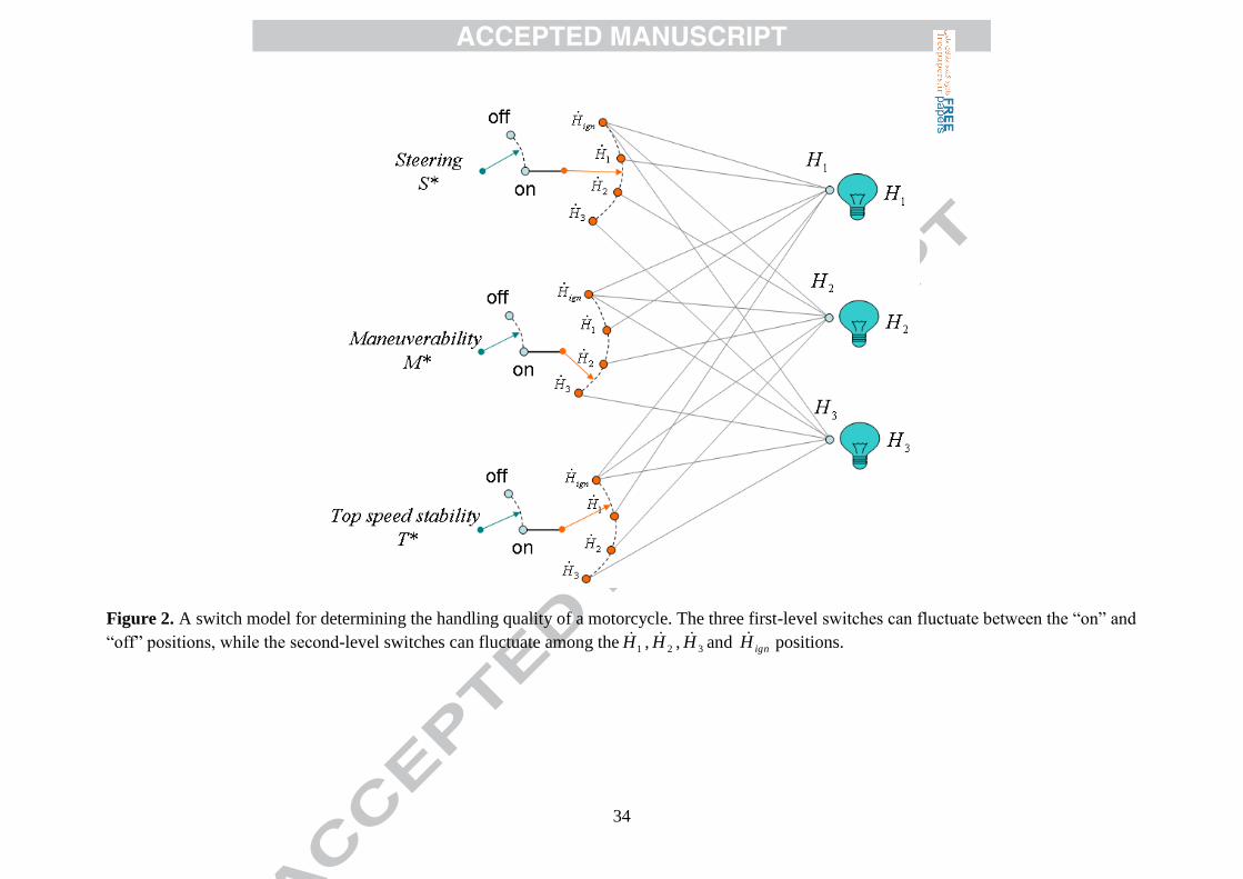
Honda. Based on Pearl’s switch metaphor and illustrated in Figure 2, one can think of each of

the three criteria as a switch independently fluctuating between the “on” and “off” positions

according to its weight wi. (We denote these switches representing the criteria as “first-level”

switches.) For example, the steering switch is at the “on” position for w1 of the time, and at

the “off” position for (1-w1) of the time. Within each criterion, a “second-level” switch

fluctuates between four possible positions ( 1H , 2H , 3H plus an “ignorance” position ignH )

according to the belief degrees given the experts. For example, the second-level switch for

the steering criterion for Honda spends 0.5 of the time at 2H , 0.3 of the time at 3H and 1-

(0.5+0.3)=0.2 of the time at ignH . In the special case illustrated in Figure 3a, the steering

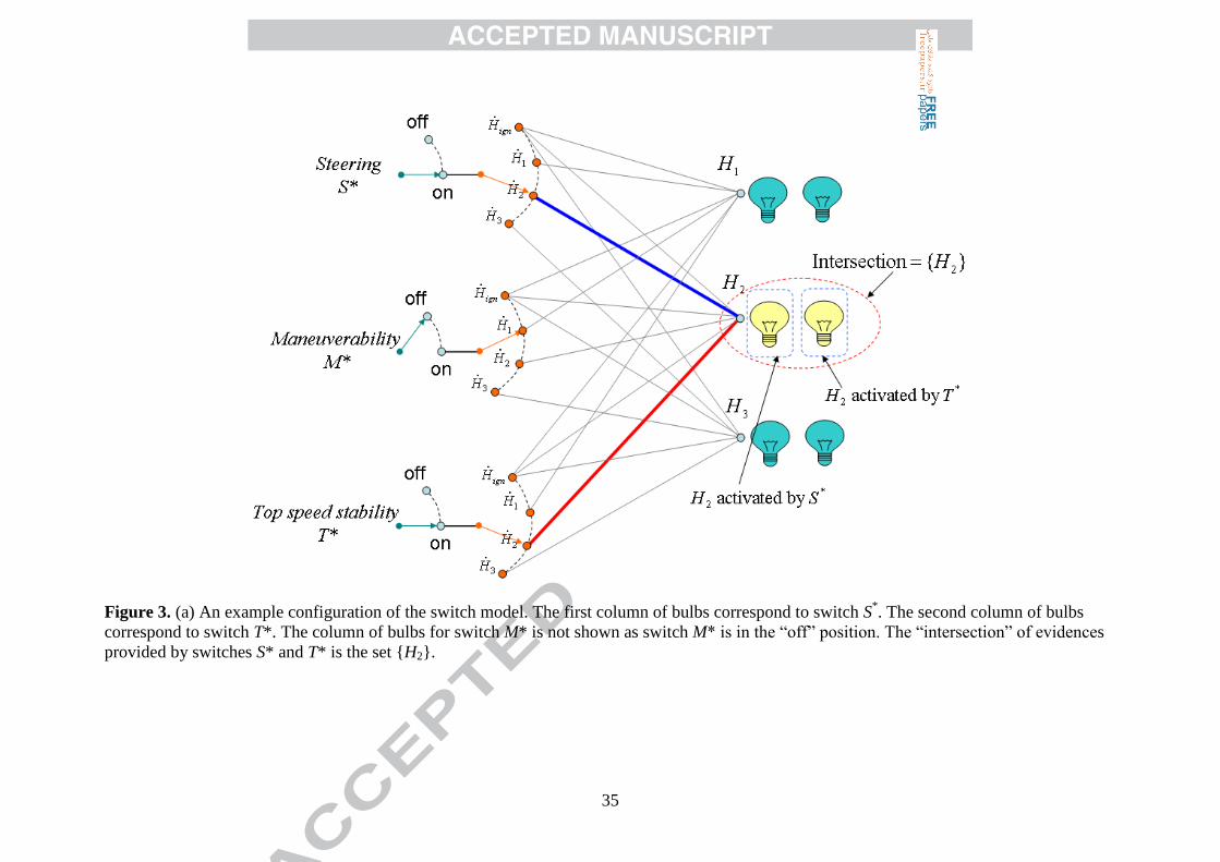
switch is “on” and the corresponding second-level switch is at 2H . Imagine an electric current

flowing from S* to 2H and finally to H2, leading the bulb at H2 to light up.

10

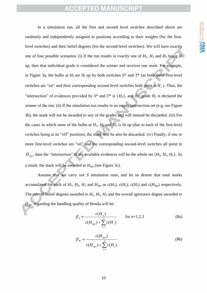
In a simulation run, all the first and second level switches described above are

randomly and independently assigned to positions according to their weights (for the first-

level switches) and their belief degrees (for the second-level switches). We will have exactly

one of four possible scenarios: (i) If the run results in exactly one of H1, H2 and H3 being lit

up, then that individual grade is considered the winner and receives one mark. For example,

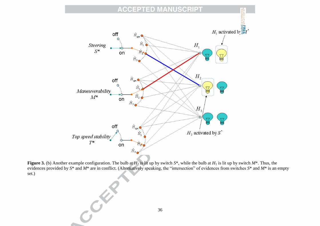
in Figure 3a, the bulbs at H2 are lit up by both switches S* and T* (as both these first-level

switches are “on” and their corresponding second-level switches both point at 2H ). Thus, the

“intersection” of evidences provided by S* and T* is {H2}, and the grade H2 is declared the

winner of the run. (ii) If the simulation run results in an empty intersection set (e.g. see Figure

3b), the mark will not be awarded to any of the grades and will instead be discarded. (iii) For

the cases in which none of the bulbs at H1, H2 and H3 is lit up (due to each of the first-level

switches being at its “off” position), the mark will be also be discarded. (iv) Finally, if one or

more first-level switches are “on” and the corresponding second-level switches all point to

ignH , then the “intersection” of the available evidences will be the whole set {H1, H2, H3}. As

a result, the mark will be awarded to Hign (see Figure 3c).

Assume that we carry out S simulation runs, and let us denote that total marks

accumulated for each of H1, H2, H3 and Hign as c(H1), c(H2), c(H3) and c(Hign) respectively.

The overall belief degrees awarded to H1, H2, H3 and the overall ignorance degree awarded to

Hign regarding the handling quality of Honda will be:

3

1

)()(

)(

i

iign

n

n

HcHc

Hc for n=1,2,3 (8a)

3

1

)()(

)(

i

iign

ign

H

HcHc

Hc (8b)

11

In other words, 1 ,.., N and H can be simply interpreted as the fractions of “non-discarded”

marks that are awarded to H1,..,HN and Hign respectively.

In summary, in a simulation run under the switch metaphor, it is the intersection of all

available evidences that is regarded as a proof that an entity under consideration be assigned

a particular grade (or set of grades) in that simulation run. On the other hand, if the available

evidences in a run lead to conflict result (i.e. the “intersection” of the available evidences is

empty), then the result of that run is discarded. Therefore, Eq.(8) follows from Pearl’s

observation that methodologies built upon Dempster-Shafer theory concern with computing

the probabilities of provability, rather than the probabilities of truth as in the standard

Bayesian framework.

3.2. Re-derivation of the analytic formulas of basic ER technique

To illustrate how the switch-metaphor based simulation framework encapsulated by

Eq.(8) can lead to the same analytic formulas derived via the formal ER framwork, let us

compute the expected number of times H1 receives marks across the S simulation runs

(denoted as )( 1Hc ). Specifically, in order for H1 to receives a mark in a run, the following

two conditions must be satisfied: (i) At least one of the three first-level switches is at its “on”

position (otherwise, the mark will be discarded according to our discussion in section 3.1); (ii)

for those first-level switches at the “on” position, at least one of the associated second-level

switches is at the 1H position while the rest of the associated second-level switches are at the

ignH position, leading to an intersection set {H1}. Equivalently, across the S simulation runs,

)( 1Hc is the number of runs in which none of the bulbs at H2 and H3 is lit up (thus a mark in

each of these runs is awarded to either H1 or Hign, or is discarded), subtracted by the number

of runs in which none of the bulbs at H1, H2 and H3 is lit up (thus a mark in each of these runs

is either awarded to Hign or discarded). Thus,

12

)}(1{)}(1{)( ,3,2,1

3

1,3,2

3

11 lllllllll wSwSHc (9)

or more general,

}1{}1{)(1 ,1,1 ,1

N

j ljl

L

l

N

njj ljl

L

ln wSwSHc (10)

when we have L criteria and N individual grades. Similarly, c(Hign) is the number of runs in

which none of the bulbs at H1, H2 and H3 is lit up, subtracted by the number of runs in which

none of the three first-level switch is on. Therefore,

}1{}1{)( 11 ,1 l

L

l

N

j ljl

L

lign wSwSHc (11)

Now, substituting Eqs.(10) and (11) into Eq.(8a) yields

}1{}1{)1(}1{

}1{}1{

}1{}1{}1{}1{

}1{}1{

1

1

,1

1 ,1

,1

1

,1

,1

,1

1

1

,1

1 1

,1

,1

,1

1

,1

,1

,1

l

L

l

N

j

ljl

L

l

N

k

N

kjj

ljl

L

l

N

j

ljl

L

l

N

njj

ljl

L

l

l

L

l

N

j

ljl

L

l

N

k

N

j

ljl

L

l

N

kjj

ljl

L

l

N

j

ljl

L

l

N

njj

ljl

L

l

n

wwNw

ww

wwww

ww

(12)

which is identical to Eq.(6a). Similarly, substituting Eqs.(10) and (11) into Eq.(8b) will lead

to Eq.(6b). Thus, the switch-metaphor based simulation framework constitutes an alternative

formulation of the basic ER technique. The simulation-based derivation of Eqs.(6a) and (6b)

arguably offers a more intuitive view of how these equations operate, compared to the

previously available mathematical induction based proof.

3.3. Re-deriving the ER technique with interval uncertainties

Recall from Section 2.2 that in the ER technique with interval uncertainties, the set of

grades available for rating an entity of interest is given by Eq.(7) and nij , is the belief degree

assigned to the grade interval Hi,j when assessing the entity with respect to the nth

criterion.

The switch model in this setting consists of the first-level switches in either the “on” or “off”

13

position, while each of the second-level switches can take on one of these positions: 1,1H ,

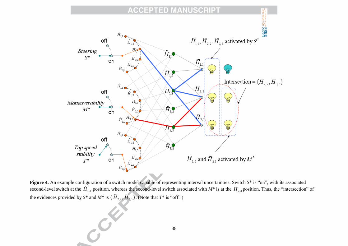
2,1H , 3,1H , 2,2H , 3,2H , 3,3H . For example, in Figure 4, the steering switch is at the “on”

position, and the associated second-level switch is at 3,1H . Imagine an electric current flowing

from S* to 3,1H and finally to 3,1H , leading the bulbs at 1,1H , 2,2H and 3,3H being lit up.

Meanwhile, the current flowing from M* to 3,2H leads to the bulbs at 2,2H and 3,3H being lit

up, while the top speed stability switch is “off”. Thus, the bulbs that are lit up by all the

available evidences are the “intersection set” },{ 3,32,2 HH , and in this case, the interval grade

H2,3 is considered as supported by all the available evidences.

Like the switch model of Section 3.1, in a simulation run, the first and second level

switches of the present switch model are assigned randomly and independently to positions

according to their weights/belief degrees. The resulting “intersection set” determines which

of 1,1H , 2,1H , 3,1H , 2,2H , 3,2H , 3,3H is the winner and receives one mark. (In the example

shown in Figure 4, 3,2H is the winner.) If the intersection set is an empty set (meaning the

available evidences lead to conflict), then the mark is discarded. Finally, if none of the bulbs

are lit up in the run due to all the first-level switches being “off”, the mark is awarded to Hign.

(Note: it is in contrast with the switch model of Section 3.2, in which the mark is discarded if

all the first-level switches are “off” in the run. As we will see next, Xu et al. make this

peculiar assumption of the mark being awarded to Hign implicitly in their paper (Xu et al.,

2006). Arguably, the simulation-based framework quite effectively brings this to light. We

will have a further remark on this at the end of this sub-section.)

Analogous to Eq.(8), the overall belief degree assigned to the grade Hi,j is

5

1

5

,

,

,

)()(

)(

p iq

qpign

ji

ji

HcHc

Hc (13a)

14

and that to Hign is

5

1

5

, )()(

)(

p iq

qpign

ign

H

HcHc

Hc (13b)

where c(Hi,j) (c(Hign)) denotes the total marks received by Hi,j (Hign) across S simulation runs.

As an illustration of how the above switch model can lead to the same formulas given

in Xu et al. (2006) for the ER technique with interval uncertainties, consider a simple case

with two criteria, and with available grades being the N=5 version of Eq.(7). The

corresponding switch model possesses two first-level switches with weights w1 and w2

respectively. In order for say H3,4 to receive a mark in a simulation run, one of the following

scenarios must occur: (i) switch 1 is “on”, and the associated second-level switch is at the

4,3H position, while switch 2 is either “off”, or if it is “on”, its associated second-level switch

must be at a position jiH , where i ≤ 3 and j ≥ 4; (ii) same as (i) but with switches 1 and 2

exchanging roles; (iii) switch 1 is “on”, with the associated second-level switch at the jH ,3

position, where j > 4, and switch 2 is also “on”, with the associated second-level switch at the

4,iH position, where i < 3; (iv) same as (iii) but with switches 1 and 2 exchanging roles. (In

essence, (i-iv) enumerate all possible scenarios in which the intersection of the available

evidences is precisely { 3,3H , 4,4H }.) Thus, across the S simulation runs, the expected number

of times H3,4 receives marks is

}-

])1[(])1[({)(

2,3421,341

2

1

5

5

1,412,32

2

1

5

5

2,421,31

3

1

5

4

1,112,342

3

1

5

4

2,221,3414,3

ww

wwww

wwwwwwSHc

i j

ij

i j

ij

i j

ij

i j

ij

(14)

15

where the term 2,3421,341 wwS corrects for the double counting occurred in (i-ii) and (iii-iv).

Meanwhile, the expected number of times Hign receives marks is when both first-level

switches are off:

)}1)(1{()( 21 wwSHc ign (15)

Substituting Eqs.(14) and (15) into Eqs.(13a) and (13b) followed by simple algebraic

manipulation will lead to the same results as captured by Eqs.(33-35) in Xu et al. (2006). The

above analysis can in principle be extended to the general case with not two but n criteria,

with care to correct for double counting. Overall, the simulation-based derivation of the ER

technique with interval uncertainties is much shorter and arguably more intuitive compared to

a previously available proof.

Incidentally, an alternative formulation of the ER approach with interval uncertainties

is to drop the “c(Hign)” term in Eq.(13a), leading to:

5

1

5

,

,

,

)(

)(

p iq

qp

ji

ji

Hc

Hc (16)

and then substituting Eq.(14) directly into the above equation. This essentially means that the

mark is discarded, instead of being awarded to Hign, if all the first-level switches are “off” in

the corresponding run. Such an alternative formulation is then consistent with that of the

basic ER approach as encapsulated by Eqs.(6) and (12), and can be considered as a correction

to the formulas given in Xu et al. (2006).

3.4. Re-deriving the ER technique with both interval and fuzzy uncertainties

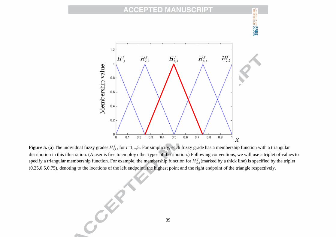
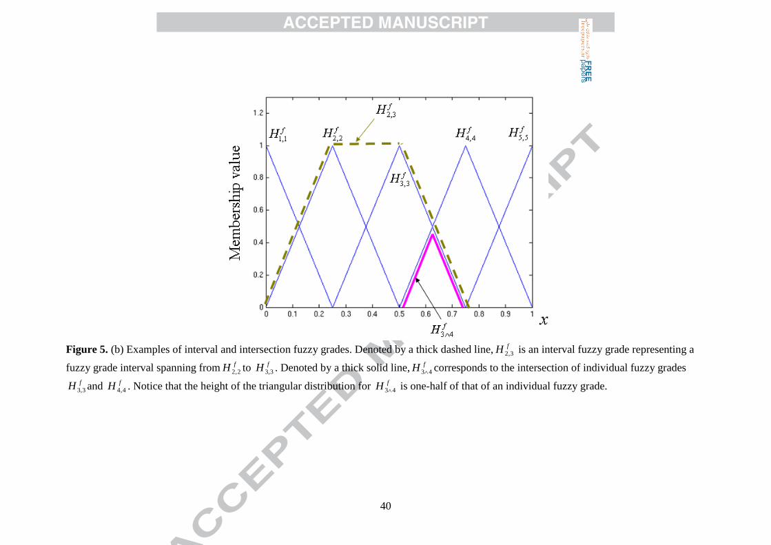
Again, recall from Section 2.2 that in the formal ER technique with both interval and

fuzzy uncertainties, each individual grade f

iiH , represents a fuzzy set (e.g. for simplicity, one

with a triangular membership function), and f

jiH , represents a fuzzy grade interval spanning

fromf

iiH , tof

jjH , . Meanwhile,f

ppH 1 corresponds to the intersection of two adjacent fuzzy

16

grades f

ppH , and f

ppH 1,1 . (See Figure 5 for an illustration.) Analogous to that of Section 3.3,

the switch model in present setting consists of the first-level switches in either the “on” or

“off” position, whereas each of the second-level switches can take on one of these positions:

fH 1,1 , fH 2,1

, fH 3,1 , fH 2,2

, fH 3,2 , fH 3,3

. Figure 6 illustrates some of the typical configurations of the

model. In particular, Figure 6a is completely analogous to Figure 4, with the resulting

“intersection set” being },{ 3,32,2

ff HH , and thus the fuzzy interval grade fH 3,2 is considered as

supported by the available evidences. On the other hand, in Figure 6b, the maneuverability

switch is at the “on” position, with the associated second-level switch at fH 2,1 , leading to fH 1,1

and fH 2,2 (denoted as set 1) being lit up; the top speed stability switch is also at the “on”

position, with the associated second-level switch at fH 3,3 , leading to fH 3,3

(denoted as set 2)

being lit up. In this case, the intersection of sets 1 and 2 is fH 2,1 ∩ fH 3,3 , i.e. fH 32 . Consequently,

the fuzzy grade fH 32 is considered supported by the available evidences.

Like the switch model discussed in Section 3.3, in a simulation run, the resulting

“intersection set” determines which one of { fH 1,1 , fH 2,1 ,.., fH 3,3 } { fH 21 , fH 32 } is the winner.

A feature different from that of Section 3.3 is that if f

jiH , (with 1≤i≤j≤3) is the winner, it will

receive the full one mark, whereas if f

iiH 1 (with i{1,2}) is the winner, then it will receive

only half a mark. (The rationale is that the intersection of adjacent triangular membership

functions leads to a triangular membership function with a height of one-half. Refer to Figure

5b. Also see Guo et al. (2009) and Yang et al. (2006) for further comments.) Other than this

difference, the rest is the similar: the mark is discarded if the intersection set is an empty set;

the mark is also discarded if none of the bulbs are lit up due to all the first-level switches

being “off”. To be consistent with Eq.(16), the overall belief degree assigned to the various

fuzzy grades can be defined as

17

2

1

1

3

1

3

,

,

,

)()(

)()(

p

f

pp

p iq

qp

f

jif

ji

HcHc

HcH (17a)

and

2

1

1

3

1

3

,

1

1

)()(

)()(

p

f

pp

p iq

qp

f

iif

ii

HcHc

HcH (17b)

where )( ,

f

jiHc (or )( 1

f

iiHc ) denotes the total marks received by f

jiH , (or f

iiH 1 ) across S

simulation runs.

Based on a derivation analogous to that described in Section 3.3 and without resorting

to logically complicated proofs, one can show that the switch model for the present setting,

together with Eq.(17), leads to the same recursive formulas as captured by Eqs.(27-42) in

Guo et al. (2009), for computing overall belief degrees in ER with interval and fuzzy

uncertainties. We will further illustrate this using an industrial dataset in Section 4.

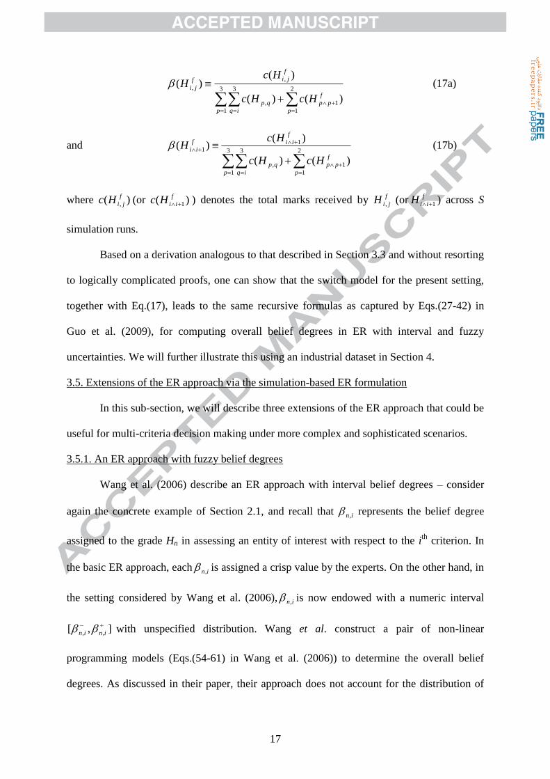
3.5. Extensions of the ER approach via the simulation-based ER formulation

In this sub-section, we will describe three extensions of the ER approach that could be

useful for multi-criteria decision making under more complex and sophisticated scenarios.

3.5.1. An ER approach with fuzzy belief degrees

Wang et al. (2006) describe an ER approach with interval belief degrees – consider

again the concrete example of Section 2.1, and recall that in, represents the belief degree

assigned to the grade Hn in assessing an entity of interest with respect to the ith

criterion. In

the basic ER approach, each in, is assigned a crisp value by the experts. On the other hand, in

the setting considered by Wang et al. (2006), in, is now endowed with a numeric interval

],[ ,,

inin with unspecified distribution. Wang et al. construct a pair of non-linear

programming models (Eqs.(54-61) in Wang et al. (2006)) to determine the overall belief

degrees. As discussed in their paper, their approach does not account for the distribution of

18

belief degrees within their corresponding intervals. Here, based on the switch model

framework, we develop an ER approach with in, ’s being allowed to take on fuzzy values.

This extended approach relies on a probabilistic linguistic computing (PLC) formulation of

fuzzy set theory (FST) (discussed fully in Ngan (2014)), the gist of which is summarized

below.

3.5.1.1. PLC formulation of fuzzy set theory

A PLC set Ω (say the concept “tall person”), like a fuzzy set, is endowed with a

membership function f , such that a given entity with an attribute value x (say the measured

height of a person) is assigned a membership value )(xfy with regard to Ω. PLC further

assumes the existence of a binary decision making context in which the probability that x is

admitted as a member of Ω under that binary decision making context is given by

)()|( xfxP . Thus, given two PLC sets Ω and Λ with the associated membership

functions f and f respectively, the intersection Ψ≡Ω∩Λ can be viewed as possessing the

membership function f such that

)(),|(

)(),|(

)|(),|()|,()(

xfxP

xfxP

xPxPxPxf

(18)

Similarly, Π ≡ ΩΛ can be viewed as possessing the membership function f such that

)(),|()()(

)(),|()()()(

xfxPxfxf

xfxPxfxfxf

(19)

Intuitively, the term P(Ω|Λ,x) can be interpreted as the probability of x being

classified as a member of Ω in a binary decision, given that x has already been classified as a

member of Λ in another binary decision. Consider the following schemes to specify P(Ω|Λ,x):

19

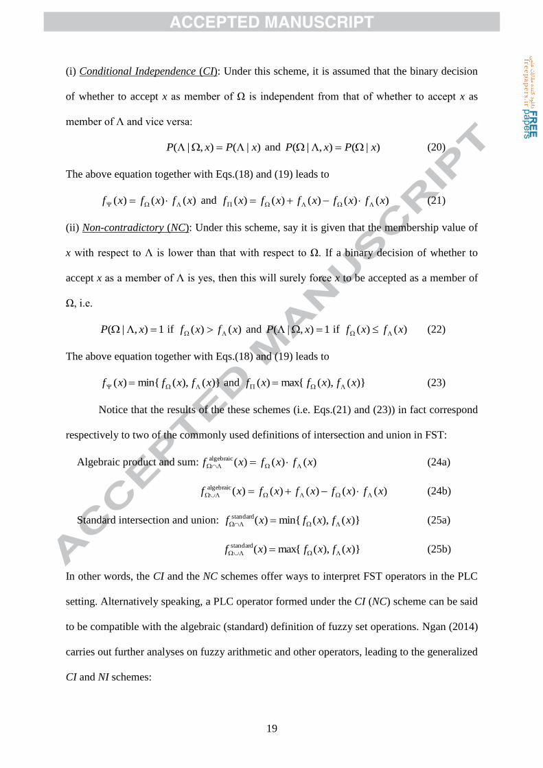
(i) Conditional Independence (CI): Under this scheme, it is assumed that the binary decision

of whether to accept x as member of Ω is independent from that of whether to accept x as

member of Λ and vice versa:

)|(),|( xPxP and )|(),|( xPxP (20)

The above equation together with Eqs.(18) and (19) leads to

)()()( xfxfxf and )()()()()( xfxfxfxfxf (21)

(ii) Non-contradictory (NC): Under this scheme, say it is given that the membership value of

x with respect to Λ is lower than that with respect to Ω. If a binary decision of whether to

accept x as a member of Λ is yes, then this will surely force x to be accepted as a member of

Ω, i.e.

1),|( xP if )()( xfxf and 1),|( xP if )()( xfxf (22)

The above equation together with Eqs.(18) and (19) leads to

)}(),(min{ )( xfxfxf and )}(),(max{ )( xfxfxf (23)

Notice that the results of the these schemes (i.e. Eqs.(21) and (23)) in fact correspond

respectively to two of the commonly used definitions of intersection and union in FST:

Algebraic product and sum: )()()(algebraic xfxfxf (24a)

)()()()()(algebraic xfxfxfxfxf (24b)

Standard intersection and union: )}(),(min{)(standard xfxfxf (25a)

)}(),(max{)(standard xfxfxf (25b)

In other words, the CI and the NC schemes offer ways to interpret FST operators in the PLC

setting. Alternatively speaking, a PLC operator formed under the CI (NC) scheme can be said

to be compatible with the algebraic (standard) definition of fuzzy set operations. Ngan (2014)

carries out further analyses on fuzzy arithmetic and other operators, leading to the generalized

CI and NI schemes:

20

(i) Generalized Conditional Independence (GCI): Given a collection of PLC sets J1,..,JN and

the corresponding attribute values j1,..,jN, then the GCI scheme requires

)|(),..,,,..,,,..,|( 1111 kKNNkkk jJPjjJJJJJP for k{2,..,N-1}

)|(),..,,,..,|( 11121 jJPjjJJJP NN

)|(),..,,,..,|( 111 NNNNN jJPjjJJJP

(ii) Generalized Non-contradictory (GNC): Given a collection of PLC sets J1,..,JN with the

associated membership function 1Jf ,..,

NJf and the corresponding attribute values j1,..,jN, we

can find an index i such that )}(),..,(min{)( 11 NJJiJ jfjfjfNi

. Then, the GNC scheme

requires 1),,|( kiik jjJJP , for any k≠i.

3.5.1.2. The ER approach under the GCI and GNC schemes

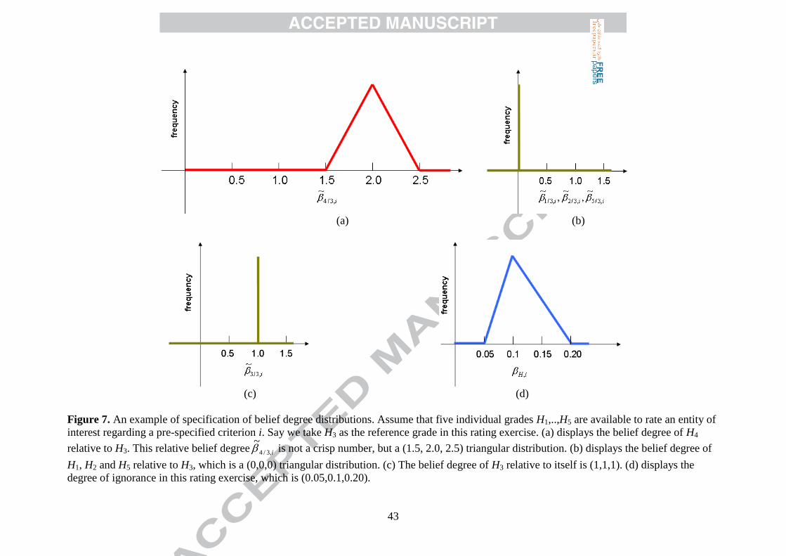
In our SB-ER approach with fuzzy belief degrees, for a given criterion i, we take one

grade, say nH (where },..,1{ Nn , with say N=5) as the reference grade, and specify the

relative belief degree of each of the other grades with respect to nH via an associated fuzzy

number – for example, in Figure 7a, H3 is the reference grade and i,3/4

~ (the belief degree of

H4 relative to H3) is a fuzzy number with a triangular membership function centered at 2.

(Thus, i,3/4

~ is regarded as a fuzzy number with its value about 2.) Furthermore, we specify

our degree of ignorance iH , with its own fuzzy number (see Figure 7d).

In leading to an ER approach with fuzzy belief degrees that is compatible with the

standard definition of the fuzzy set operations, we use the switch model to carry out one set

of simulation runs as follows: (i) Random crisp values inm ,/̂ and iH ,̂ , associated with the

relative belief degrees inm ,/

~ ’s and the ignorance degree iH , , are jointly generated as

specified by the GNC scheme. (Specifically, we generate a candidate set of random crisp

values inm ,/̂ and iH ,̂ from the uniform distribution. This set of crisp values is to be jointly

accepted as members of the associated fuzzy sets inm ,/

~ and iH , with a probability of

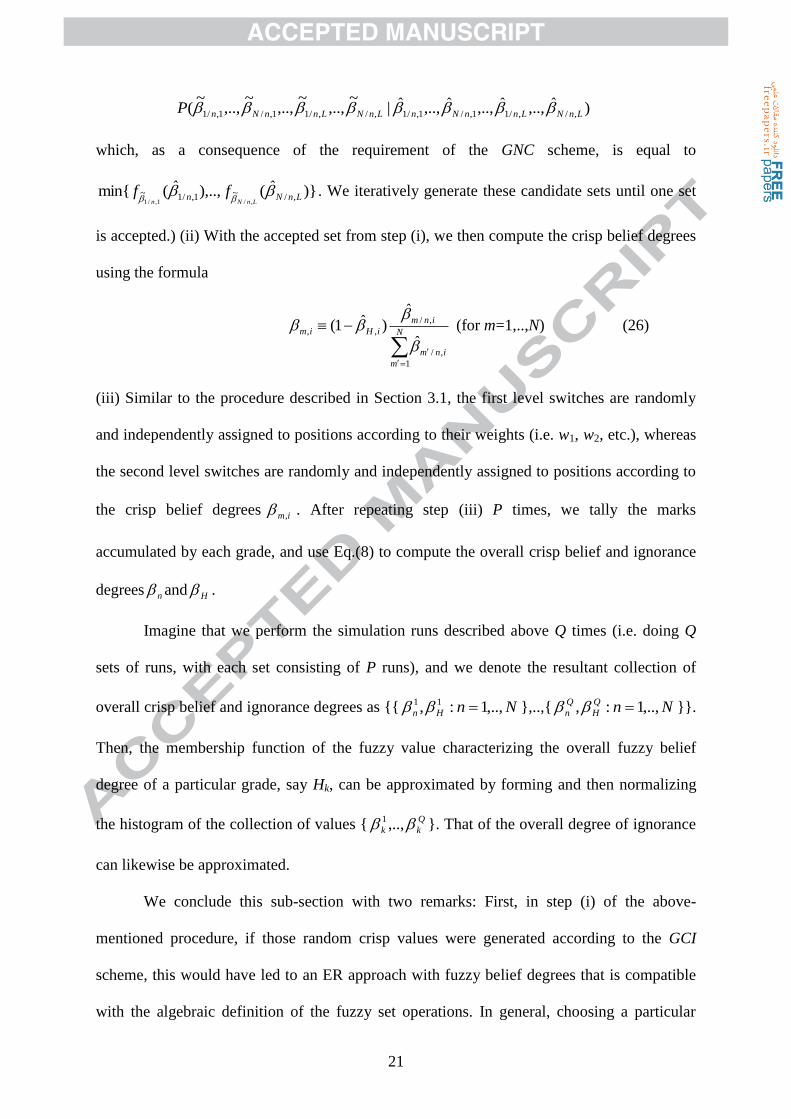
21

)ˆ,..,ˆ,..,ˆ,..,ˆ|~

,..,~

,..,~

,..,~

( ,/,/11,/1,/1,/,/11,/1,/1 LnNLnnNnLnNLnnNnP

which, as a consequence of the requirement of the GNC scheme, is equal to

)}ˆ(),..,ˆ(min{ ,/~1,/1~,/1,/1

LnNnLnNn

ff

. We iteratively generate these candidate sets until one set

is accepted.) (ii) With the accepted set from step (i), we then compute the crisp belief degrees

using the formula

N

m

inm

inm

iHim

1

,/

,/

,,

ˆ

ˆ)ˆ1(

(for m=1,..,N) (26)

(iii) Similar to the procedure described in Section 3.1, the first level switches are randomly

and independently assigned to positions according to their weights (i.e. w1, w2, etc.), whereas

the second level switches are randomly and independently assigned to positions according to

the crisp belief degrees im, . After repeating step (iii) P times, we tally the marks

accumulated by each grade, and use Eq.(8) to compute the overall crisp belief and ignorance

degrees n and H .

Imagine that we perform the simulation runs described above Q times (i.e. doing Q

sets of runs, with each set consisting of P runs), and we denote the resultant collection of

overall crisp belief and ignorance degrees as {{ NnHn ,..,1:, 11 },..,{ NnQ

H

Q

n ,..,1:, }}.

Then, the membership function of the fuzzy value characterizing the overall fuzzy belief

degree of a particular grade, say Hk, can be approximated by forming and then normalizing

the histogram of the collection of values { Q

kk ,..,1 }. That of the overall degree of ignorance

can likewise be approximated.

We conclude this sub-section with two remarks: First, in step (i) of the above-

mentioned procedure, if those random crisp values were generated according to the GCI

scheme, this would have led to an ER approach with fuzzy belief degrees that is compatible

with the algebraic definition of the fuzzy set operations. In general, choosing a particular

22

conditional dependence schemes can lead us to an ER approach compatible with a particular

definition of FST operations. Second, the present approach involves the standard grades {Hn:

n=1,..,N}. On the other hand, it is straightforward to extend it to model interval and fuzzy

grades, by combining the present switch model with the switch model depicted in Section 3.4.

In principle, the above modifications and extensions can be accomplished without carrying

out any logically complicated derivation or proof.

3.5.2. An ER approach with conditional dependencies among the belief degrees

In a more sophisticated scenario, it may be desirable to have the capability to model

conditional dependence relations among in, ’s and iH , . For instance, consider the following

situation: A decision maker may be uncertain about the precise rating for the ith

criterion of a

given entity, thus offering of a belief degree of 0.5 to grade H2, and a belief degree of 0.4 to

grade H3. Likewise, she might have the same ambivalence about the jth

criterion for the entity,

again giving the belief degrees of 0.5 and 0.4 to grades H2 and H3 respectively with regard to

criterion j. However, she may happen to believe criteria i and j to be so intimately related for

the given entity that the ratings for both criteria should jointly be of either grade H2 or grade

H3. In terms of the switch model, this means that in any simulation run, it is forbidden to have

a configuration in which the second level switch for criterion i points to H2 while that for

criterion j points to H3.

In general, in the switch model language, the conditional dependence relation across

two criteria i and j can be fully specified by the following set of values: (i) )( ni HCP – the

probability that the second level switch for criterion i points to nH in a simulation run (in

particular, we have inni HCP ,)( ); (ii) )|( nimj HCHCP – the probability that the

switch for criterion j points to mH , given that the switch for criterion i points to nH in that

simulation run. With this set of values prescribed by the decision maker, one performs a set

23

of P simulation runs as follows. In each run: (i) The first level switches are randomly and

independently assigned to positions according to their weights; (ii) The second level switches

are randomly assigned to their positions according to their joint probability distribution as

specified by the )( ni HCP and )|( nimj HCHCP values. After repeating steps (i) and

(ii) P times, the marks accumulated by each grade are tallied. Finally, Eq.(8) can be used to

compute the overall belief and ignorance degrees n and H .

3.5.3. An ER approach with hesitancies in the belief degrees

In the present formal ER approach, with in, representing the belief degree assigned to

the grade Hn in assessing an entity with respect to the ith

criterion, the residual value

(

N

n in1 ,1 ) is relegated as the degree of ignorance H. In a more informative scenario, a

decision maker might not necessarily want to cast away this residual value entirely to H. For

example, on top of assigning a belief degree of 0.5 to grade Hn, he may also assign a degree

of disbelief of 0.3 to grade Hn, thus implying a degree of hesitancy of (1-0.5-0.3)=0.2 towards

Hn. Thus, this type of formulation can be viewed as integrating the concept of intuitionistic

fuzzy set (Atanassov 1986, 1994) into ER.

As it will take substantial space to fully explore the various possible formulations of

ER with hesitancies in the belief degrees, we will simply describe a bare switch model here,

and leave the derivations of the analytical results and further discussions elsewhere. Briefly,

in a simulation run: (i) The first level switches are randomly and independently assigned to

positions according to their weights wi’s; (ii) Random value ri, drawn from a uniform

distribution between 0 and 1, is independently generated for each second level switch i.

Based on ri, the second level switch for criterion i will be assigned to one of the following

positions: (a) fully to one of nH ’s (with n{1,..,N}, where N is the number of available

individual grades), (b) hesitantly to one of nH , or (c) fully to ignH . Now, in a simulation run,

24

if the “intersection” of the evidences results in a singleton set {Hn}, then a mark is to be

assigned to the grade Hn either fully (in which case all the second level switches in that run

have been fully assigned to their respective positions), or hesitantly (i.e. at least one of the

second level switches in that run has been hesitantly assigned to its position). After

performing P runs of steps (i) and (ii), we tally the marks (distinguishing the fully assigned

marks from the hesitantly assigned marks) accumulated by each grade. We then normally the

marks appropriately to obtain the overall degree of belief and the overall degree of hesitancy

of each grade for our entity of interest.

3.6. Further remarks

To close this section, we give a short illustration on (i) how the simulation-based

framework can handle cases in which there are more than two levels of attributes, and (ii)

how to aggregate belief structures in which the focal elements are allowed to be arbitrary

subsets of singleton grades.

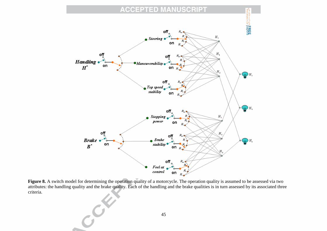
Regarding (i), again emulating an example from Yang & Xu (2002) regarding

motorcycle assessment, let us assume that a super-attribute operation quality of a motorcycle

comprises of two attributes: the handling quality and the brake quality. As mentioned in the

preceding sub-sections, the handling quality attribute comprises of three criteria: steering,

maneuverability and top speed stability. Following Yang & Xu (2002), the brake quality

attribute is assumed to comprise of the criteria stopping power, braking stability, and feel at

control. Then, Figure 2 can be extended to become Figure 8. Suppose that the weights of the

handling quality and brake quality for assessing the operation super-attribute are whandling and

wbrake respectively. Then, similar to our discussion in Section 3.1, the switch for the handling

quality will be at the “on” position for whandling of the time, and at the “off” position for (1-

whandling) of the time, while the switch for the brake quality will be “on” for wbrake of the time,

and “off” for (1-wbrake) of the time. In a simulation run, if the positions of the switches in

25

Figure 8 happen to be assigned in such a way that there is a complete path from say H* (or B

*)

to a light bulb, then that light bulb will be designated as “on”. We then use the same rules as

described in Section 3.1 either to assign the mark associated with that simulation run to a

“winner” grade, or to discard the mark.

Figure 4 can be extended analogously, allowing multi-level modeling of attributes

with interval and fuzzy uncertainties. Furthermore, complex topology (e.g. one in which an

attribute has n levels of sub-attributes, while another attribute has m levels of sub-attributes,

with m≠n) can be easily constructed and analyzed via the simulation-based framework.

Regarding (ii), Xu (2012) points out that while ER has been extended to handle

interval uncertainties (i.e. a focal element can be any subset of adjacent singleton grades,

such as H2,3, as illustrated in Eq.(7) and fully discussed in Xu et al. (2006)), ER has not yet

been developed to handle uncertainties in which the focal element can be a subset of any

combination of singleton grades, such as (H1, H3). It is further pointed out that “such

extension could be quite challenging.” Here, it can be shown that the switch model can

readily implement this type of extension. Again, as it will take non-negligible space to fully

explore and analyze the consequences, we will illustrate this extension briefly with a short

example: Consider Figure 2, and imagine in a simulation run, all the first level switches are

on. Further suppose that the second level switch of S*

happens to take on both positions 1H

and 3H (i.e. having two arrows pointing at 1H and 3H respectively), while that of M* takes

on position 1H and that of T* also on 1H . Then, the “intersection” of the evidences provided

by S*, M

* and T

* is the set {H1} and the mark for that run would be awarded to the grade H1.

Instead, if each of the second level switches for S*, M

* and T

* point to both 1H and 3H , then

the intersection of the evidences would become the set {H1, H3} and the mark would be

awarded to the focal element (H1, H3). After performing a sufficient number of simulation

runs and tallying the marks accumulated by each subset of the singleton grades, the overall

26

belief degree for each subset can be determined by appropriately normalizing the marks. In

principle, one can also derive analytic formulas for the overall belief degrees based on this

extended switch model.

4. RESULTS AND DISCUSSIONS

In order to illustrate and validate the methods discussed in Section 3, we now apply

the switch-model simulation-based ER approaches to a small industrial engineering dataset

extracted from Yang & Xu (2002). Specifically, we desire to evaluate the overall engine

quality of four types of motorcycles; the five criteria used to assess the engine quality are

quietness, fuel efficiency, responsiveness, vibration and starting. Table 2, which reproduces

part of Table III in Yang & Xu (2002), describes the weights of the criteria as well as the

ratings given by the experts to these motorcycles.

The switch model of Section 3.1, designed to mimic the basic formal ER approach, is

run repeatedly for 3 million times (run-time ≈ 48 sec. under the Matlab environment on an

Intel duo-core 2.33GHz CPU) for each of the four motorcycle types, and by applying Eq.(8)

to the outcomes of the runs, we obtain the results displayed in Table 3a. These numeric

results closely approximate the analytical results (Table 3b) obtained via Eq.(6). The mean

relative error, determined by the formula

}3b and 3a Tables in theentries zero-non{ 3b Table from

3b Table from3a Taable from

)(

)()(1

mMRE (27)

to average over the relative error of the corresponding pairs of non-zero entries from Tables

3a and 3b (where m is the number of non-zero entries in Table 3b), is 0.24%.

To validate the switch model of Section 3.4 (designed to mimic the formal ER

approach with both interval and fuzzy uncertainties), let us modify Table 2, such that each

individual grade Hi is replaced by a corresponding fuzzy gradef

iiH , with a triangular

membership function (see Figure 5 again for illustration). Furthermore, we modify some of

27

the ratings given by the experts to allow for the introduction of “interval-fuzzy” grades,

resulting in Table 4. Based on the new table, the switch model of Section 3.4 is run for 3

million times (run-time ≈ 48 sec.), again for each of the motorcycle types. By applying

Eq.(17) (but with n=5 instead of n=3), we obtain the results detailed in Table 5, which closely

approximate the results (Table 6) obtained by applying recursive formulas described in

Eqs.(27-42) in (Guo et al., 2009) to the dataset. The mean relative error in this case is 0.23%.

Thus, the above numerical experiments give further evidence about the utility of SB-

ER for approximating the answers the formal ER approach would have given. For practical

purposes, when a closed form formula for a case under investigation is readily available from

the formal ER approach, it will be most efficient to use that formula directly to obtain an

answer for the case. For other cases (such as situations with relations among the attributes

and sub-attributes forming complex topologies), it would be more efficient to use SB-ER to

obtain an answer, bypassing the need to derive complicated analytic formulas.

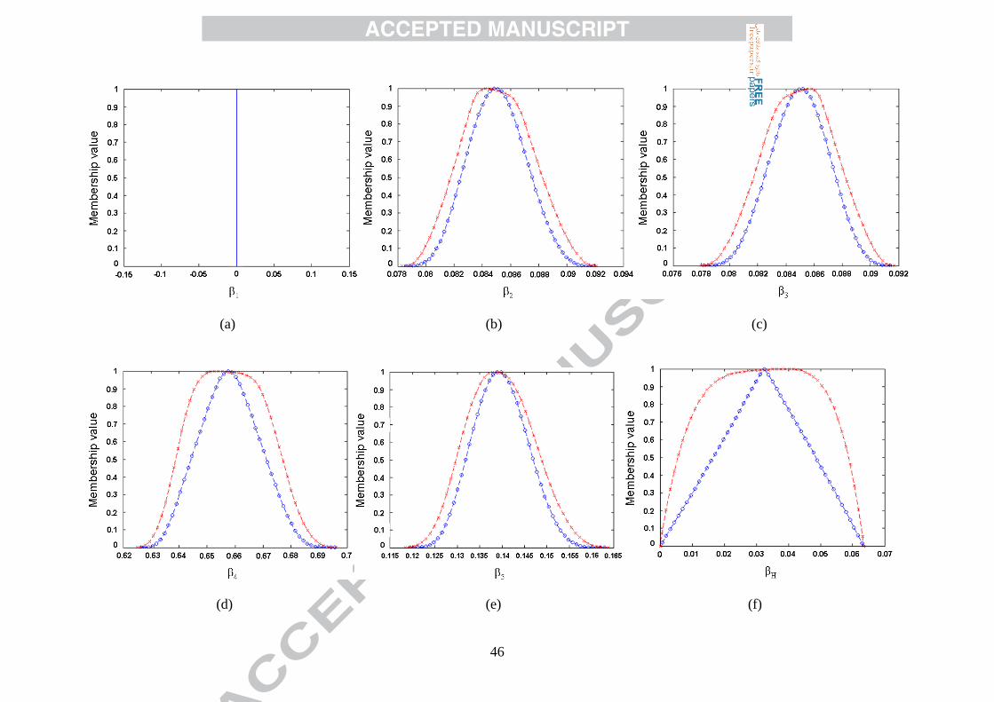
To illustrate the utility of the switch model representing the new ER approach that

allows for fuzzy belief degrees (described in Section 3.5.1), let us modify Table 2, such that

the ratings take on the distribution as depicted in Table 7. By collecting the outcomes from

the runs, the membership functions of fuzzy numbers, representing the overall belief degrees

for the engine quality of Honda, are obtained and displayed in Figure 9 (the results for the

other three motorcycle types not displayed to conserve space). Specifically, the dashed lines

with circles are the resulting fuzzy numbers obtained under the GCI scheme (thus compatible

with the algebraic definition of fuzzy set operations), whereas the lines with crosses are those

obtained under the GNC scheme (thus compatible with the standard definition of fuzzy set

operations).

Finally, to illustrate the utility of the switch model that can account for the possibility

of conditional dependencies among the belief degrees (described in Section 3.5.2), let us

28

create a new table (Table 8), showing three scenarios for rating a given motorcycle across

five criteria. In particular, Table 8a shows no conditional dependencies across the criteria,

whereas Tables 8b and c show different extents of dependencies. We note from Table 8 that

the resulting overall belief degrees are different for these three different scenarios, and the

extended switch model is capable of correctly accounting for these differences.

As mentioned in Sections 3.5.3 and 3.6, further discussions of the switch models

allowing for hesitancies and for arbitrary sets of singleton grades will be presented elsewhere.

5. CONCLUSION

As evidenced by its application to a wide range of domains from engineering design

and safety assessment to policy making and business management, the Evidential Reasoning

(ER) approach is among the premier methods for multiple-criteria decision making. A key

weakness in the existing ER framework is that its formulation usually involves complex

formulas with logically non-trivial proofs. This complexity may either require a non-

specialist to use ER as a black-box technique, or cause him/her to become hesitant to use ER

altogether. In this article, we have applied the random-switch metaphor of J. Pearl (Pearl,

1988) to recast ER into a simulation-based framework. As a consequence, its inner working

has become much easier for the non-specialists to understand. For the specialists, the

simulation-based framework offers an alternative perspective to view the theoretical

landscape of ER. Based on this perspective, future theoretical extensions of ER can be greatly

facilitated. More specifically, in this article, we have demonstrated that the simulation-based

ER approach can lead us to the same analytic formulas previously derived from the formal

ER approach, and through examples, we have illustrated the ease of extending the capability

of the existing ER approach via the simulation-based framework. In essence, owing its

intellectual debt to both the formal ER approach and the Pearl’s switch metaphor, the

simulation-based framework significantly removes the complexity encountered in the

29

existing ER framework, reveals a logically straightforward way to comprehend the inner

working of ER, and paves a promising shortcut for fine-tuning and further developing ER. A

set of Matlab source codes for SB-ER, complementing existing formal ER-based software

packages such as Intelligent Decision System (Xu & Yang (2003); Xu, McCarthy & Yang

(2006)), is available from the author upon request.

For future work, we currently engage in integrating the simulation-based ER approach

with other existing MCDM techniques. Specifically, building upon the insightful suggestions

in Xu (2012), we are reanalyzing and expanding the combined Dempster-Shafer theory

(DST)-Analytic Hierarchy Process (AHP) approach of Beynon (2000), as well as the

combined DST-outranking approach of Amor et al. (2007), based on the switch model.

Another direction of research is the re-examination and extensions of the axiomatic works

originated by Yang & Xu (2002). As Xu (2012) points out, a source of nonlinearity in ER

originates from the observation that harmonic evidence tends to strengthen relevant beliefs

larger than the simple sum of beliefs, whereas conflicting evidence leads to the opposite

effect. In the switch model context, this observation can be concretely traced to the fact that

the award of a mark in a simulation run is not being distributed proportionally according to

the amount of “votes” a grade receives in that run, but rather, the “winner” grade of that run

(according to the way a “winner” is defined under the current rules of SB-ER) receives the

whole mark. Thus, by modifying the way in which a mark is to be distributed to the

individual grades, one can obtain a whole spectrum of ER-based MCDM methods, with

“simple-averaging” schemes residing at one end of the spectrum and “winner-takes-all”

schemes residing at the other end. In this sense, it may become highly feasible to examine the

rationality and to unearth the concrete underlying meaning of a proposed information

aggregation rule for evidential reasoning using the switch model.

30

REFERENCES

Amor, S. B., Jabeur, K., & Martel, J. M. (2007). Multiple criteria aggregation procedure for

mixed evaluations. European Journal of Operational Research, 181, 1506–1515.

Atanassov, K.T. (1986). Intuitionistic fuzzy sets. Fuzzy Sets and Systems, 20, 87-96.

Atanassov, K.T. (1994). New operations defined over the intuitionistic fuzzy sets. Fuzzy Sets

and Systems, 61, 137-142.

Beynon, M., Curry, B., & Morgan, P. (2000). The Dempster-Shafer theory of evidence: an

alternative approach to multicriteria decision modelling. Omega, 28, 37–50.

Chin, K.S., Yang, J.B., Guo, M. & Lam, J.P.K. (2009). An evidential-reasoning-interval-

based method for new product design assessment. IEEE Transactions on Engineering

Management, 56, 142-156.

Graham, G. & Hardaker, G. (1999). Contractor evaluation in the aerospace industry: using

the evidential reasoning approach. Journal of Research in Marketing &

Entrepreneurship, 3(3), 162-173.

Guo, M., Yang, J.B., Chin, K.S. & Wang, H.W. (2007). Evidential reasoning based

preference programming for multiple attribute decision analysis under uncertainty.

European Journal of Operational Research, 182(3), 1294–1312.

Guo, M., Yang, J.B., Chin, K.S., Wang, H.W. & Liu, X.B. (2009). Evidential reasoning

approach for multiattribute decision analysis under both fuzzy and interval uncertainty.

IEEE Transactions on Fuzzy Systems, 17, 683-697.

Hilhorst, C., Ribbers, P., Heck, E.V. & Smits, M. (2008). Using Dempster-Shafer theory and

real options theory to assess competing strategies for implementing IT infrastructures:

a case study. Decision Support Systems, 46(1), 344–355.

Kabak, Ö. & Ruan, D. (2011). A cumulative belief degree-based approach for missing values

in nuclear safeguards evaluation. IEEE Transactions on Knowledge and Data

Engineering, 23(10), 1441-1454.

Liu, J., Ruan, D., Wang, H. & Martinez, L. (2009). Improving IAEA safeguards evaluation

through enhanced belief rule-based inference methodology. International Journal of

Nuclear Knowledge Management, 3, 312–339.

Martinez, L., Liu, J., Ruan, D. & Yang, J.B. (2007). Dealing with heterogeneous information

in engineering evaluation processes. Information Sciences, 177, 1533–1542.

Ngan, S.C. (2014). Revisiting fuzzy set and fuzzy arithmetic operators and constructing new

operators in the land of probabilistic linguistic computing. Submitted.

Pearl, J. (1988). Probabilistic reasoning in intelligent systems: networks of plausible

inference. San Mateo, CA: Morgan Kaufmann.

Ren, J., Yusuf, Y.Y. & Burns, N.D. (2009). A decision-support framework for agile

enterprise partnering. The International Journal of Advanced Manufacturing

Technology, 41, 180–192.

Saaty, T.L. (1988). The analytic hierarchy process: University of Pittsburgh.

Shafer, G.A. (1976). Mathematical theory of evidence. Princeton: Princeton University Press.

Sonmez, M., Graham, G., Yang, J.B. & Holt, G.D. (2002). Applying evidential reasoning to

pre-qualifying construction contractors. Journal of Management in Engineering, 18(3),

111–119.

Tanadtang, P., Park, D. & Hanaoka, S. (2005). Incorporating uncertain and incomplete

subjective judgments into the evaluation procedure of transportation demand

management alternatives. Transportation, 32(6), 603–626.

Wang, Y.M., Yang, J.B. & Xu, D.L. (2006). Environmental impact assessment using the

evidential reasoning approach. European Journal of Operational Research, 174, 1885–

1913.

31

Wang, Y.M., Yang, J.B. & Xu, D.L. (2006). The evidential reasoning approach for multiple

attribute decision analysis using interval belief degrees. European Journal of

Operational Research, 175(1), 35-66.

Xu, D.L. (2012). An introduction and survey of the evidential reasoning approach for

multiple criteria decision analysis. Annals of operations research, 195, 163–187.

Xu, D.L., McCarthy, G. & Yang, J.B. (2006). Intelligent decision system and its application

in business innovation self assessment. Decision Support Systems, 42, 664–673.

Xu, D.L. & Yang, J.B. (2003). Intelligent decision system for self-assessment. Journal of

Multi-Criteria Decision Analysis, 12, 43–60.

Xu, D.L., Yang, J.B. & Wang, Y.M. (2006). The ER approach for multi-attribute decision

analysis under interval uncertainties. European Journal of Operational Research,

174(3), 1914–1943.

Yang, J.B. & Sen, P. (1994). A general multi-level evaluation process for hybrid MADM

with uncertainty. IEEE Transactions on Systems, Man, and Cybernetics, 24(10),

1458-1473.

Yang, J.B. & Singh, M.G. (1994). A evidential reasoning approach for multiple attribute

decision making with uncertainty. IEEE Transactions on Systems, Man, and

Cybernetics, 24(1), 1-18.

Yang, J.B., Wang, Y.M., Xu, D.L. & Chin, K.S. (2006). The evidential reasoning approach

for MCDA under both probabilistic and fuzzy uncertainties. European Journal of

Operational Research, 171(1), 309–343.

Yang, J.B. & Xu, D.L. (2002). On the evidential reasoning algorithm for multiple attribute

decision analysis under uncertainty. IEEE Transactions on Systems, Man and

Cybernetics. Part A. Systems and Humans, 32(3), 289–304.

Yang, J.B., Xu, D.L., Xie, X.L. & Maddulapalli, A.K. (2011). Multicriteria evidential

reasoning decision modelling and analysis—prioritising voices of customer. Journal

of the Operational Research Society, 62(9), 1638–1654.

Yao, R. & Zheng, J. (2010). A model of intelligent building energy management for the

indoor environment. Intelligent Buildings International, 2, 72–80.

Zhang, Z.J., Yang, J.B. & Xu, D.L. (1989). A hierarchical analysis model for multiobjective

decision making. In: Analysis, design and evaluation of man-machine system,

selected papers from the 4th IFAC/IFIP/IFORS/IEA conference. Xian, China:

Pergamon, Oxford.

32

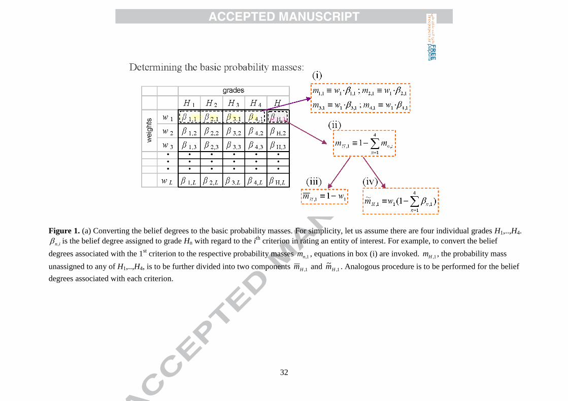
Figure 1. (a) Converting the belief degrees to the basic probability masses. For simplicity, let us assume there are four individual grades H1,..,H4.

in, is the belief degree assigned to grade Hn with regard to the ith

criterion in rating an entity of interest. For example, to convert the belief

degrees associated with the 1st criterion to the respective probability masses 1,nm , equations in box (i) are invoked. 1,Hm , the probability mass

unassigned to any of H1,..,H4, is to be further divided into two components 1,Hm and 1,~

Hm . Analogous procedure is to be performed for the belief

degrees associated with each criterion.

33

Figure 1. (b) Combining the basic probability masses to determine overall belief degrees. inI , keeps track of the un-normalized belief degree

assigned to grade Hn so far (i.e. by accounting for the basic probability masses from the first to the ith

criterion). Thus, inI , ’s first get initialized in

box (i). In box (ii), we iteratively account for the basic probability masses starting from the first and finally to the Lth

criterion. In box (iii), the

resulting un-normalized belief degrees LnI , and LnI ,

~are normalized, leading to the overall belief degrees for the individual grades as well as the

overall degree of ignorance.

34

Figure 2. A switch model for determining the handling quality of a motorcycle. The three first-level switches can fluctuate between the “on” and

“off” positions, while the second-level switches can fluctuate among the 1H , 2H , 3H and ignH positions.

35

Figure 3. (a) An example configuration of the switch model. The first column of bulbs correspond to switch S*. The second column of bulbs

correspond to switch T*. The column of bulbs for switch M* is not shown as switch M* is in the “off” position. The “intersection” of evidences

provided by switches S* and T* is the set {H2}.

36

Figure 3. (b) Another example configuration. The bulb at H2 is lit up by switch S*, while the bulb at H1 is lit up by switch M*. Thus, the

evidences provided by S* and M* are in conflict. (Alternatively speaking, the “intersection” of evidences from switches S* and M* is an empty

set.)

37

Figure 3. (c) A third example configuration. Switches S* and T* are “on”, with their respective second-level switches both at the ignH position.

(M* is “off”.) Bulbs at H1, H2 and H3 are lit up by both switches S* and T*. Thus, the “intersection” of evidences from S* and T* is the whole set

of grades H={H1, H2, H3}.

38

Figure 4. An example configuration of a switch model capable of representing interval uncertainties. Switch S* is “on”, with its associated

second-level switch at the 3,1H position, whereas the second-level switch associated with M* is at the 3,2H position. Thus, the “intersection” of

the evidences provided by S* and M* is { 2,2H , 3,3H }. (Note that T* is “off”.)

39

Figure 5. (a) The individual fuzzy grades f

iiH , , for i=1,..,5. For simplicity, each fuzzy grade has a membership function with a triangular

distribution in this illustration. (A user is free to employ other types of distribution.) Following conventions, we will use a triplet of values to

specify a triangular membership function. For example, the membership function forfH 3,3 (marked by a thick line) is specified by the triplet

(0.25,0.5,0.75), denoting to the locations of the left endpoint, the highest point and the right endpoint of the triangle respectively.

40

Figure 5. (b) Examples of interval and intersection fuzzy grades. Denoted by a thick dashed line, fH 3,2 is an interval fuzzy grade representing a

fuzzy grade interval spanning fromfH 2,2 to

fH 3,3 . Denoted by a thick solid line, fH 43 corresponds to the intersection of individual fuzzy grades

fH 3,3 and fH 4,4 . Notice that the height of the triangular distribution for fH 43 is one-half of that of an individual fuzzy grade.

41

Figure 6. (a) An example configuration of a switch model capable of representing interval and fuzzy uncertainties. Bulbs at fH 1,1

, fH 2,2 ,

fH 3,3 are

lit up by switch S*, leading to the trapezoidal membership functionfH 3,1 ; Bulbs at

fH 2,2 ,

fH 3,3 are lit up by switch M*, leading to the trapezoidal

membership functionfH 3,2 . (T* is off.) Thus, the “intersection” of the evidences provided by S* and M* is

fH 3,2 .

42

Figure 6. (b) Another example configuration of the switch model. Bulbs atfH 1,1 ,

fH 2,2 are lit up by switch M*, leading to the trapezoidal

membership functionfH 2,1 ; Bulb at

fH 3,3 is lit up by switch T*, leading to the triangular membership function

fH 3,3 . Thus, the “intersection” of the

evidences provided by M* and T* is fH 32 .

43

(a) (b)

(c) (d)

Figure 7. An example of specification of belief degree distributions. Assume that five individual grades H1,..,H5 are available to rate an entity of

interest regarding a pre-specified criterion i. Say we take H3 as the reference grade in this rating exercise. (a) displays the belief degree of H4

relative to H3. This relative belief degree i,3/4

~ is not a crisp number, but a (1.5, 2.0, 2.5) triangular distribution. (b) displays the belief degree of

H1, H2 and H5 relative to H3, which is a (0,0,0) triangular distribution. (c) The belief degree of H3 relative to itself is (1,1,1). (d) displays the

degree of ignorance in this rating exercise, which is (0.05,0.1,0.20).

45

Figure 8. A switch model for determining the operation quality of a motorcycle. The operation quality is assumed to be assessed via two

attributes: the handling quality and the brake quality. Each of the handling and the brake qualities is in turn assessed by its associated three

criteria.

46

(a) (b) (c)

(d) (e) (f)

47

Figure 9. The overall belief degrees regarding the engine quality of a motorcycle. The raw data for Honda from Table 7 is used to generate these

graphs. (a-f) show the membership functions of the associated fuzzy numbers representing the overall belief degrees of H1,.., H5 and of the

degree of ignorance Hign respectively. The dashed lines with circles are the results obtained under the GCI scheme, whereas those with crosses

are the results obtained under the GNC scheme. Note that β1 is actually the crisp number 0.

48

Kawasaki Honda

steering w1 H1(0.5), H2(0.5) H2(0.5), H3(0.3)

maneuverability w2 H2(1.0) H1(0.5), H2(0.5)

top speed stability w3 H3(0.8) H3(1.0)

Criteria weightsMotorcycle types

Table 1. The ratings for the handling quality of two motorcycle types by the experts. The handling quality is assessed by three criteria: steering,

maneuverability and top speed stability. The grades H1, H2, H3 stand for below average, average, and good respectively. The value inside the

parenthesis after a grade indicates the corresponding belief degree. For example, the steering of Honda is rated average with a belief degree of

0.5 and good with a belief degree of 0.3.

49

Kawasaki Honda Yamaha BMW

quietness w1=0.2 H2(0.5), H3(0.5) H4(0.5), H5(0.3) H3(1.0) H5(1.0)

fuel efficiency w2=0.2 H3(1.0) H2(0.5), H3(0.5) H2(1.0) H5(1.0)

responsiveness w3=0.2 H5(0.8) H4(1.0) H4(0.3), H5(0.6) H2(1.0)

vibration w4=0.2 H4(1.0) H4(0.5), H5(0.5) H2(1.0) H1(1.0)

starting w5=0.2 H4(1.0) H4(1.0) H3(0.6), H4(0.3) H3(1.0)

Criteria weightsMotorcycle types

Table 2. The ratings for the engine quality of four motorcycle types by the experts.

50

degree of ignorance

β1 β2 β3 β4 β5 βH

Kawasaki 0 0.09328 0.30494 0.42242 0.14370 0.03567

Honda 0 0.08535 0.08490 0.65769 0.13957 0.03248

Yamaha 0 0.41881 0.32363 0.11256 0.10889 0.03611

BMW 0.19038 0.18987 0.19072 0 0.42903 0

belief degreesMotorcycle types

(a)

degree of ignorance

β1 β2 β3 β4 β5 βH

Kawasaki 0 0.09385 0.30503 0.42235 0.14302 0.03575

Honda 0 0.08503 0.08503 0.65785 0.13969 0.03239

Yamaha 0 0.41926 0.32268 0.11307 0.10908 0.03592

BMW 0.19048 0.19048 0.19048 0 0.42857 0

belief degreesMotorcycle types

(b)

Table 3. The overall belief degrees and the overall degrees of ignorance of the four motorcycle types. (a) displays the values determined from

the simulation of the switch model described in Section 3.2. (b) displays the values computed using the analytical formulas (Eq.(6)).

51

Kawasaki Honda Yamaha BMW

quietness w1=0.2 Hf2,3(1.0) H

f4,5(0.8) H

f3,3(1.0) H

f5,5(1.0)

fuel efficiency w2=0.2 Hf3,5(1.0) H

f2,2(0.5), H

f3,3(0.5) H

f2,3(1.0) H

f5,5(1.0)

responsiveness w3=0.2 Hf5,5(0.8) H

f4,5(1.0) H

f4,4(0.3), H

f5,5(0.6) H

f2,3(1.0)

vibration w4=0.2 Hf4,5(1.0) H

f4,5(0.5) H

f2,2(1.0) H

f1,2(1.0)

starting w5=0.2 Hf2,4(1.0) H

f4,4(1.0) H

f3,3(0.6), H

f4,4(0.3) H

f3,3(1.0)

Criteria weightsMotorcycle types

Table 4. The modified ratings for the engine quality of the four motorcycle types, so that interval and fuzzy grades are incorporated.

52

β(Hfi,j)

i = 1i = 2i = 3i = 4i = 5

β(HfjΛj+1) 0 0.04291 0.03223 0.00345

00.09630

0

0.03063000

0.09333

j = 4 j = 5

00.19869

00.15857

00

0

j = 1 j = 2 j = 3

000

0.3439000

0000

(a) Kawasaki

β(Hfi,j)

i = 1i = 2i = 3i = 4i = 5

β(HfjΛj+1)

00000

j = 1 j = 2 j = 3

000

0.0811700

j = 4 j = 5

00.08156

00

0

0

0

0.26930

0

0.09964

0

0

0.42500

0

0 0 0.04333 0

(b) Honda

Table 5. The overall belief degrees and the overall degrees of ignorance of the four motorcycle types. These values are determined using the

simulation of the switch model of Section 3.4.

53

β(Hfi,j)

i = 1i = 2i = 3i = 4i = 5

β(HfjΛj+1)

00000

j = 1 j = 2 j = 3

000

0.0441100

j = 4 j = 5

00

00.17642

0

0.14082

0.03539

0.04405

0

0.02687

0

0.14044

0.17622

0.16729

0 0 0.02741 0.02100

(c) Yamaha

β(Hfi,j)

i = 1i = 2i = 3i = 4i = 5

β(HfjΛj+1)

00000

j = 1 j = 2 j = 3

000

0.2120500

j = 4 j = 5

0.169200.04238

00.16874

0

0

0

0

0

0

0

0

0

0.38130

0 0.02634 0 0

(d) BMW

Table 5. (cont’d)

54

β(Hfi,j)

i = 1i = 2i = 3i = 4i = 5

β(HfjΛj+1)

00000

j = 1 j = 2 j = 3

000

0.3438300

j = 4 j = 5

00.19855

00.15884

000

0.096380

0.03062000

0.09298

0 0.04298 0.03242 0.00340

(a) Kawasaki

β(Hfi,j)

i = 1i = 2i = 3i = 4i = 5

β(HfjΛj+1) 0 0 0.04338 0

0

0.26895

0

0.09984

0

0

0.42516

0

j = 4 j = 5

00.08133

00

0

0

0

j = 1 j = 2 j = 3

000

0.0813300

0000

(b) Honda

Table 6. The overall belief degrees and the overall degrees of ignorance of the four motorcycle types. These values are computed using the

recursive formulas (Eqs.(27-42)) in Guo et al. (2009).

55

β(Hfi,j)

i = 1i = 2i = 3i = 4i = 5

β(HfjΛj+1) 0 0 0.02751 0.02096

0.03521

0.04401

0

0.02683

0

0.14084

0.17605

0.16767

j = 4 j = 5

00

00.17605

0

0.14084

0

j = 1 j = 2 j = 3

000

0.0440100

0000

(c) Yamaha

β(Hfi,j)

i = 1i = 2i = 3i = 4i = 5

β(HfjΛj+1) 0 0.02646 0 0

0

0

0

0

0

0

0

0.38095

j = 4 j = 5

0.169310.04233

00.16931

0

0

0

j = 1 j = 2 j = 3

000

0.2116400

0000

(d) BMW

Table 6. (cont’d)

56

H1 H2 H3 H4 H5 βH,i

quietness w1=0.2 (0,0,0) (0,0,0) (0,0,0) (0,0,0) (1,1,1) (0,0,0)

fuel efficiency w2=0.2 (0,0,0) (0,0,0) (0,0,0) (0,0,0) (1,1,1) (0,0,0)

responsiveness w3=0.2 (0,0,0) (1,1,1) (0,0,0) (0,0,0) (0,0,0) (0,0.3,0.5)

vibration w4=0.2 (1,1,1) (0,0,0) (0,0,0) (0,0,0) (0,0,0) (0,0,0)

starting w5=0.2 (0,0,0) (0,0,0) (1,1,1) (0,0,0) (0,0,0) (0,0,0)

Criteria weightsBMW

H1 H2 H3 H4 H5 βH,i

quietness w1=0.2 (0,0,0) (0,0,0) (1,1,1) (0,0,0) (0,0,0) (0,0,0)

fuel efficiency w2=0.2 (0,0,0) (1,1,1) (0,0,0) (0,0,0) (0,0,0) (0,0,0)

responsiveness w3=0.2 (0,0,0) (0,0,0) (0,0,0) (1,1,1) (1.5,2,2.5) (0.0,0.1,0.3)

vibration w4=0.2 (0,0,0) (1,1,1) (0,0,0) (0,0,0) (0,0,0) (0,0,0)

starting w5=0.2 (0,0,0) (0,0,0) (1,1,1) (0.3,0.5,0.7) (0,0,0) (0.0,0.1,0.3)

Criteria weightsYamaha

H1 H2 H3 H4 H5 βH,i

quietness w1=0.2 (0,0,0) (1,1,1) (0.9,1,1.1) (0,0,0) (0,0,0) (0,0,0)

fuel efficiency w2=0.2 (0,0,0) (0,0,0) (1,1,1) (0,0,0) (0,0,0) (0,0,0)

responsiveness w3=0.2 (0,0,0) (0,0,0) (0,0,0) (0,0,0) (1,1,1) (0.1,0.2,0.3)

vibration w4=0.2 (0,0,0) (0,0,0) (0,0,0) (1,1,1) (0,0,0) (0,0,0)

starting w5=0.2 (0,0,0) (0,0,0) (0,0,0) (1,1,1) (0,0,0) (0,0,0)

Criteria weightsKawasaki

H1 H2 H3 H4 H5 βH,i

quietness w1=0.2 (0,0,0) (0,0,0) (0,0,0) (1,1,1) (0.5,0.6,0.7) (0,0.2,0.4)

fuel efficiency w2=0.2 (0,0,0) (1,1,1) (0.9,1,1.1) (0,0,0) (0,0,0) (0,0,0)

responsiveness w3=0.2 (0,0,0) (0,0,0) (0,0,0) (1,1,1) (0,0,0) (0,0,0)

vibration w4=0.2 (0,0,0) (0,0,0) (0,0,0) (1,1,1) (0.9,1,1.1) (0,0,0)

starting w5=0.2 (0,0,0) (0,0,0) (0,0,0) (1,1,1) (0,0,0) (0,0,0)

Criteria weightsHonda

Table 7. The modified ratings for the engine quality of the four motorcycle types, so that belief degrees can take on fuzzy values. For example, in the

“quietness” row of Honda, H4 serves as the reference grade, and the grade H5 has the average relative belief degree of 0.6 with respect to H4. Moreover, this

relative belief degree takes on a fuzzy value, whose membership function is a triangular distribution with parameters (0.5,0.6,0.7). Meanwhile, the degree of

ignorance regarding the quietness of Honda takes on a fuzzy value with triangular distribution with parameters (0,0.2,0.4).

57

responsiveness w1=0.2 H4(0.3), H5(0.5)

fuel efficiency w2=0.2 H2(0.9)

quietness w3=0.2 H1(0.5), H2(0.4)

vibration w4=0.2 H1(0.5), H2(0.4)

starting w5=0.2 H3(0.3), H4(0.5)

Criteria weights Ratings

degree of ignorance

β1 β2 β3 β4 β5 βH

Overall rating 0.2030 0.3679 0.0560 0.1561 0.0934 0.1237

belief degreesMotorcycle types

Table 8. (a) The ratings for the engine quality of a given motorcycle by an expert. This expert assumes no conditional dependencies of belief

degrees across the different criteria. The bottom box shows the resultant overall belief degrees.

58

Table 8. (b) The ratings for the engine quality of a given motorcycle by another expert. In rating this motorcycle, the expert assumes conditional

dependencies of belief degrees between the criteria responsiveness and starting, as well as between quietness and vibration. The bottom box

shows the resultant overall belief degrees.

59

Table 8. (c) Likewise, in rating the given motorcycle, this expert assumes conditional dependencies of belief degrees between the criteria

responsiveness and starting, as well as between quietness and vibration, though the extent of dependencies is different from that shown in (b).

The bottom box shows the resultant overall belief degrees.

60

Highlights:

The Evidential Reasoning (ER) approach is among the premier methods for MCDM.

The existing ER framework involves complex formulas with non-trivial proofs.

We recast ER into a simulation-based framework, termed SB-ER.

This framework enables straightforward comprehension of the inner working of ER.

Moreover, the existing ER approach can be readily extended via the SB-ER framework.