Evidence on Structural Instability in - Princeton …mwatson/papers/Stock_Watson_JBES_19… · Evidence on Structural Instability in ... Structural stability; Time- varying parameters.

Evidence on Structural Instability in

Macroeconomic Time Series Relations

James H. STOCK Kennedy School of Government, Harvard University, Cambridge, MA 02138

Mark W. WATSON Woodrow Wilson School, Princeton University, Princeton, NJ 08544

An experiment is performed to assess the prevalence of instability in univariate and bivariate macroeconomic time series relations and to ascertain whether various adaptive forecasting techniques successfully handle any such instability. Formal tests for instability and out-of-sample forecasts from 16 different models are computed using a sample of 76 representative U.S. monthly postwar macroeconomic time series, constituting 5,700 bivariate forecasting relations. The tests for instability and the forecast comparisons suggest that there is substantial instability in a significant fraction of the univariate and bivariate autoregressive models.

KEY WORDS: Break tests; Forecasting; Recursive least squares; Structural stability; Time- varying parameters.

Time series econometrics typically involves drawing inferences about the present or future using historical data. In some cases these inferences are about the operation of the economy or economic policy. For example, much empirical work on monetary economics currently rests on inferences drawn from so-called structural vector autoregressions (VAR's); Bernanke and Blinder (1992) and Christiano, Eichenbaum, and Evans (in press) provided two recent ex- amples. In other cases these inferences are in the form of forecasts. Both applications require the model to be stationary in some sense (that the future be like the past) for such inferences to be valid. For example, using a structural VAR to advise policymakers requires that the historically estimated model remain relevant. Although studies occa- sionally include some analysis of stability, it is often limited in scope, perhaps consisting of reestimating the model on a single subsample. The importance of stability and the current lack of systematic evidence on it therefore leads us to ask: How generic is instability in multivariate time series relations?

To answer this, we undertake a two-part experiment. The first part assesses the prevalence of parameter instability in economic time series relations using a battery of recently developed tests for instability. This is done using a sample of 76 monthly time series for the postwar U.S. economy over the period 1959:1-1993:12 (420 observations), among which are 5,700 distinct (but not independent) bivariate forecasting relations. These series are chosen to provide relations that are representative of those of interest to macroeconomists and macroeconomic forecasters. This sample is then used to compute empirical distributions of various tests for structural stability, including Nyblom's (1989) test for parameter stability, cumulative sum (CUSUM) tests, and tests for discrete breaks such as the Quandt (1960) likelihood ratio (QLR) statistic.

The second part of the experiment examines whether current state-of-the-art adaptive forecasting models capture the instability found by the stability tests and thereby im-

prove on more naive forecasts. This entails the empirical evaluation of different forecasting models that exhibit different degrees of adaptivity, ranging from no adaptivity (fixed-parameter models) through moderate adaptivity [recursive least squares, rolling regression, and random- walk coefficient time-varying parameter (TVP) models with small coefficient evolution] to high adaptivity (TVP models with large coefficient evolution). Although work on regression models with stochastically time-varying parameters (or "stochastic coefficients") dates to Cooley and Prescott (1973a,b, 1976), Rosenberg (1972, 1973), and Sarris (1973), and although TVP models have been applied to selected series, we know of no systematic evidence on whether these techniques might be widely useful in economic forecasting applications. [Applications of adaptive forecasting include those of Baudin, Nadeau, and Westlund (1984), Guy- ton, Zhang, and Foutz (1986), Engle, Brown, and Stern (1988), Sessions and Chatterjee (1989), Schneider (1991), Young, Ng, Lane, and Parker (1991), Zellner, Hong, and Min (1991), Edlund and Sogaard (1993), Min and Zellner (1993), and the time-varying VAR's developed by Doan, Litterman, and Sims (1984), Highfield (1986), and Sims (1982, 1993). Surveys of TVP models were provided by Chow (1984), Nichols and Pagan (1985), Engle and Watson (1987), and Harvey (1989).]

Eight univariate models are considered for each of the 76 series for a total of 608 univariate forecasting equations, and eight bivariate models are considered for each of the 5,700 bivariate forecasting relations for a total of 45,600 bivariate forecasting equations. Models are com- pared using one-month-ahead mean squared errors (MSE's), computed over the (pseudo) out-of-sample period 1979:1- 1993:12. In the spirit of Makridakis et al. (1982) and Meese and Geweke (1984), who applied univariate fore-

Q 1996 American Statistical Association

Journal of Business & Economic Statistics January 1996, Vol. 14, No. 1

11

12 Journal of Business & Economic Statistics, January 1996

casting techniques to large numbers of series, this part of this experiment yields a forecasting comparison suggesting which models typically do best in macroeconomic applications. The results provide an opportunity to assess model robustness by identifying models that successfully guard against the most severe out-of-sample forecasting failures. These statistics also permit direct estimation of a paramet- ric measure of instability in the TVP model, the relative scale of the innovation in the coefficients. In a constant- parameter model, this ratio, denoted by A, is 0.

Looking ahead to the results, the tests indicate that instability is widespread. For example, the QLR test rejects stability (at the 10% level) in more than 55% of the 5,700 bivariate relations. This instability is more prevalent in certain classes of series, such as price indexes, than in others. Similarly, in over half the pairs, random-walk TVP models or rolling regressions perform better than fixed-coefficient or recursive least squares models, although these gains typically are small. In a small fraction of the cases, the TVP and recursive least squares models perform well but the fixed-coefficient models perform quite poorly, and in this sense the TVP and recursive least squares models are more robust than the fixed-coefficient models. Finally, the estimates of A, and the implied distribution of A, suggest that, although perhaps half the relations are essentially stable, a substantial fraction of relations exhibit considerable instability.

The outline of the article is as follows. The data set is described in Section 1. The stability tests are described in Section 2, the forecasting models are described in Section 3, and the methods for estimating the TVP parameter A are described in Section 4. The empirical results for the stability tests are given in Section 5, and the empirical results for the forecasting models and estimates of A are given in Section 6. Section 7 concludes.

1. THE DATA SET

Our objective in constructing the data set was to ob- tain a sample of economic time series for the United States that is representative of the relations of primary concern to macroeconomists and macroeconomic forecasters. Al- though one could in principle draw series at random from a large macroeconomic data base, a simple random sample would oversample certain classes of heavily represented series, such as industry-specific deflators, interest rates, or financial flows. Moreover, such a sample would omit important forecasting variables that are constructed from the primary data, such as interest-rate spreads. Stratification could eliminate the firstbut not the second problem.

Our sample of series therefore was obtained by apply- ing subjective judgment, using four criteria as guidelines: (1) The sample should include the main monthly economic aggregates and coincident indicators. This resulted in the inclusion of series such as industrial production, weekly hours, personal income, and inventories. (2) The sample should include important leading economic indicators. This led us to include series such as monetary quantity aggregates, interest rates, interest-rate spreads, stock prices, and

consumer expectations. (3) The series should represent different broad classes of variables that can be expected to have quite different time series properties. (4) The series should have consistent historical definitions or, when the definitions are inconsistent (e.g., different base years for different segments of a real series) it should be possible to adjust the series with a simple additive or multiplicative splice.

These criteria were used to select 76 monthly U.S. economic time series. Most of the raw data were obtained from the CITIBASE data base, although many series were sub- sequently modified (e.g., by creating interest-rate spreads). The series can be grouped into eight categories-output and sales, employment, new orders, inventories, prices, interest rates, money and credit, and other miscellaneous series including exchange rates, government spending and taxes, and miscellaneous leading indicators. The series are listed in the Appendix.

The sample runs from 1959:1 to 1993:12 (four series on government finance start in 1967:6). Each series was screened to detect breaks and outliers due to changes in definitions or reporting practice. Most series were also transformed to be approximately integrated of order 0 by taking either first differences or first differences of logarithms. For consistency, the same transformation was in general applied to entire classes of series. For example, production, employment, prices, and money were all transformed using first differences of logarithms, and interest rates were transformed by first differencing. Some series that did not fit naturally into a broader category were an- alyzed on a case-by-case basis using visual inspection, a priori reasoning, and unit-root test statistics and then transformed accordingly. The transformation for each series is listed in the Appendix. It should be emphasized that many of the procedures are only slightly affected by the use of first differences versus levels. In particular, the forecasting models produce similar short-run forecasts using levels or first differences (this would not be the case if there were bivariate cointegration, but there are neither theoret- ical nor empirical reasons to suspect widespread bivariate cointegration among these series, except perhaps for some interest-rate and inflation spreads).

2. STABILITY TESTS: METHODOLOGY

The empirical analysis uses variants of three classes of tests for parameter stability-tests for random (time- varying) coefficients, tests based on cumulative forecast errors (CUSUM tests), and tests based on sequential Wald tests for a single break. For completeness, we briefly summarize these tests here (in addition to the original references, see also Hackl and Westlund 1989, 1991; Stock 1994). The general model considered is

Yt = 't + at(L)yt-1 + it(L)xt-1 + Et, (1)

where at(L) and /3t(L) are pth-order lag polynomials that in general are time varying and where et is serially uncorrelated with mean 0 and E(c2 ytl, ... , yt-p, xt-1, ... , Xt-p)

= 2. Let k denote the total number of regressors. Each

Stock and Watson: Structural Instability in Macroeconomic Time Series Relations 13

test has as its null hypothesis that the parameters are constant; that is, pt = p, at(L) = a(L) and 3t3(L) = fl(L). The derivation of the null distributions of the test statistics also assumes that the regressors are jointly second-order stationary, along with additional technical conditions. When the following discussion refers to univariate tests, it is under- stood that the terms in xt-1 in (1) are omitted.

2.1 Tests for Time-varying Parameters

The first set of tests for randomly time-varying coefficients are Nyblom's (1989) locally most powerful tests against the alternative that the coefficients follow a random walk. Let Ot = (pt, at, .i... , at,ft,.. ., pft)' have dimension k and zt =

(1,yt-1,...IYt-pXt-1-...IXt--p)/. The random-walk TVP model is

Yt = O1zt + Et (2a)

and

Ot = Op-1 + rt, rt iid (0, A2a2Q), Er-tEt = 0 all t, k, (2b)

where Q is a k x k covariance matrix. Following Nyblom (1989), we set Q = (Eztz')-1. With this normalization, the coefficients on the transformed regressors (Eztz ) -1/2Zt follow a k-dimensional standard random walk and A2 is the ratio of the variance of each (transformed) parameter disturbance to the variance of the regression error et.

Nyblom's statistic for testing A = 0 in (2) against A # 0 is

T L = T-2 StV'-1St, (3)

t=1

where St = s=l z,e,, where {e,} are the residuals from ordinary least squares (OLS) estimation of (1), and where

S

= (T-1 -T ztz;)c2, where 2 T-T1 ••T=1 et. A heteroscedasticity-robust variant of the Nyblom statistic, denoted L', was also computed by replacing V with V

= T-1 Efl e2ztz' (Hansen 1990). The Breusch-Pagan (1979) (BP) Lagrange multiplier test

for random coefficients, for which the alternative hypothesis is that the coefficients are iid draws from a distribution with constant mean and finite variance, was also computed. The BP statistic is

TR2 from the regression of e 2

onto (1, y2)1, )...), Yt-p Xt-1 ,"' , IX2t-p). (4)

2.2 Tests Based on Cumulative Forecast Errors

One of the tests based on cumulative forecast errors is the maximal OLS CUSUM statistic proposed by Ploberger and Kriimer (1992), which is similar to Brown, Durbin, and Evans's (1975) CUSUM statistic except that the Ploberger- Kriimer statistic is computed using OLS rather than recursive residuals. Let CT(6) =

o-1T-1/2 -[T e], where [] is the greatest lesser integer function. The Ploberger-Krimer

maximal CUSUM statistic is

PKsup = sup ICT(6)I. (5) se [0,1]

A related statistic is the mean square of (T:

PKmsq = - T(S)2 dS. (6)

The PKsup and PKmsq statistics, respectively, have limiting representations as the supremum and the integral of the square of a one-dimensional Brownian bridge.

2.3 Tests Based on Sequential Wald Statistics

The third set of test statistics consists of functionals of the sequence of Wald test statistics, FT(S), which test the null hypothesis that the parameters are constant against the alternative that they have a single break at a fraction 6 through the sample. The break date is treated as unknown a priori so that the tests involve computing the sequence FT(t/T) for t = to,...I, t1 and then computing a functional of this sequence. Three such functionals are considered. The Quandt (1960) likelihood ratio statistic, in Wald form, is given by

QLR = sup FT(6). (7) 6E(6o,61)

The mean Wald statistic (Andrews and Ploberger 1994; Hansen 1992) is

61

MW = FT(6) d6. (8) o

The Andrews-Ploberger (1994) average exponential Wald statistic, in Wald form with flat weight function, is

EW=lnIn exp I

FT(6) db . (9)

These statistics have asymptotic representations as functionals of a k-dimensional Brownian bridge; see Andrews (1993) and Andrews and Ploberger (1994) for the details. The tests are implemented with 15% symmetric trimming (Ao = 1 - 61 = .15).

Heteroscedasticity-robust versions of the QLR, MW, and EW statistics (denoted QLR', MWr, and EW') were computed by replacing FT(6) in (7)-9) with F (6), where F (6) is computed using the White (1980) heteroscedasticity-robust covariance matrix, in which the residuals were computed under the null rather than each of the alternatives for computational convenience.

2.4 Monte Carlo Critical Values and Power

In case the asymptotic distributions discussed in Sec- tions 2.1-2.3 provide poor approximations to the finite- sample distributions, we generated finite-sample critical values for the L, QLR, MLR, and EW test statistics and their heteroscedasticity-robust counterparts. The distributions were computed under the null of parameter stability and under the alternative that the parameters follow the random-walk TVP model (2). The design was constructed


to capture the possible heteroscedasticity in the actual data set.

The pseudodata for the experiment were generated according to the following algorithm: (a) A pair of series (x, y) was drawn randomly with replacement from the 5,700 bivariate relations in our data base; (b) y was regressed (by OLS) against a constant and lags of y and x, yield- ing the estimated coefficients 00o; (c) a time series {Or} was generated according to the TVP model (2b), where

o00 is set to 80 and rlt are pseudorandom iid N(0, A2Q0"2), where = (T-1 ETz1 zz)-'; (d) an artificial time series Yt was generated according to it = upt + at(L)?t-1 + Ot(L)xt-1 + et, where et is iid N(0, a2); and (e) the test statistics were computed for the pair (x, y). The same algorithm was used for simulating the null distribution of the univariate tests, except that x was omitted.

To compute the null distribution and the Monte Carlo critical values, A was set to 0 for 6,000 repetitions. In addition, results were computed for 10,000 draws of A from a uniform [0, .0275] distribution, and for 1,000 draws each on a grid of A = {.0025, .005,.0075, .01,.015, .02}. These draws were used to compute the power functions and, as described in Section 4, to estimate A and its distribution.

3. FORECASTING MODEL COMPARISON: METHODOLOGY

Forecasting Models

The next stage in this investigation is an examination of the performance of 16 forecasting models, 8 univariate and 8 bivariate. Throughout, a (pseudo) in-sample estimation period is used for preliminary estimation of the parameters and a (pseudo) out-of-sample period is used for forecasting.

The eight univariate models consist of a fixed-parameter autoregression, two autoregressions estimated by rolling regression, one autoregression estimated by recursive least squares, and four random-walk TVP models. The eight multivariate models are a fixed-parameter bivariate model, two bivariate models estimated by rolling regression, one model estimated by recursive least squares, and four bivariate models with random-walk time TVP. All models are of the form (1), with the coefficients fixed or time-varying as appropriate. The bivariate models will be referred to as vector autoregressions (VAR's), although, because only one- step-ahead forecasts are considered, only the single equa- tion (1) of the (yt, xt) VAR needs to be estimated.

The specification of the TVP models is conventional and is given in (2). The parameters of the TVP models are 0o, a2, and A. The TVP models were initialized using a diffuse prior (0o = 0, state covariance matrix set to 4lk, where n is large); however, the out-of-sample forecasts and their relative performances are insensitive to choice of initial conditions because of the long in-sample period. One- step-ahead forecasts Ytlt-1 are then produced using period- by-period updating with the Kalman filter. We consider four TVP models that differ only in their choice of A.

All models were estimated with fixed lag lengths 1, 3, and 6. The models were also estimated using data-dependent

lag lengths with a lag selection procedure appropriate for the method of estimation of 0 for that model. For the TVP models, the choice of p was limited to 1, 3, or 6 for computational reasons, but for the other models p was chosen among {0, 1,..., 12}. For the fixed-parameter model, p was chosen by Bayes information criterion (BIC) for the in- sample period. For the rolling models, p was reestimated at each date by BIC using the data for the rolling period at hand, and for the recursive models p was reestimated at each date by BIC using the recursive sample. For the TVP models, p was chosen by minimizing the (conditional) predictive least squares (PLS) criterion, PLS = ET=to (Yt - YtIt-1)2 (Rissanen 1986), which is asymptotically equivalent to BIC in the stochastic regression model under certain conditions (Wei 1992) but does not explicitly involve p. To reduce de- pendence of PLS on initial conditions, the value to = 60 was used.

TVP models were estimated over a grid of A = {0, .0025, .005, .0075, .01, .015, .02}. In addition to forecasts for fixed A, TVP forecasts were computed for A chosen in each period to minimize the (recursive) PLS criterion.

Results are tabulated for eight univariate and eight bivariate models:

AR: AR; u, a(L) estimated by OLS, then fixed at in- sample values for out-of-sample forecasts, p chosen by in-sample BIC.

RRA1: AR estimated using rolling regression with 120 observations, p chosen by rolling BIC.

RRA2: AR estimated using rolling regression with 240 observations, p chosen by rolling BIC.

RLSA: AR estimated by recursive least squares, p chosen by recursive BIC.

ATVPI: AR estimated by TVP with A = .0025, p chosen by recursive PLS.

ATVP2: AR estimated by TVP with A = .0075, p chosen by recursive PLS.

ATVP3: AR estimated by TVP with A = .015, p chosen by recursive PLS.

ATVP4: AR estimated by TVP with A, p chosen by recursive PLS.

VAR: VAR; p, a(L), P(L) estimated by OLS, then fixed at in-sample values for out-of-sample forecasts, p chosen by in-sample BIC.

RRVI: VAR estimated using rolling regression with 120 observations, p chosen by rolling BIC.

RRV2: VAR estimated using rolling regression with 240 observations, p chosen by rolling BIC.

RLSV: VAR estimated by recursive least squares, p chosen by recursive BIC.

VTVPI: VAR estimated by TVP with A = .0025, p chosen by recursive PLS.


VTVP2: VAR estimated by TVP with A = .0075, p chosen by recursive PLS.

VTVP3: VAR estimated by TVP with A = .015, p chosen by recursive PLS.

VTVP4: VAR estimated by TVP with A, p chosen by recursive PLS.

Results for fixed-p models and TVP models with other values of A will be discussed briefly but not tabulated.

For the forecast comparisons, the in-sample period ends in 1978:12. This cutoff date was chosen so that the models are tested in the turbulent economic conditions of the late 1970s and early 1980s. For series ending in 1993:12, 180 observations remain for the out-of-sample comparison. In all cases, forecasts of yt+l during the out-of-sample period were computed as true forecasts in the sense that they use data only through time t.

4. ESTIMATION OF A AND THE DISTRIBUTION OF A

The parameter A determines the magnitude of the coefficient variation in the TVP model and, within this model, provides a measure of the instability in these relations. This section first outlines two procedures for estimating A. The resulting distribution of estimates of A, however, will not in general be a good estimator of a hypothesized population distribution of A. We therefore proceed to describe a deconvolution procedure that uses the distribution of estimates of A to estimate the distribution of A.

4.1 Estimation of A

For a given model (univariate or bivariate pair), we consider two sets of estimators of A. The first set consists of median unbiased estimators based on the QLR and QLR' stability tests. It was shown by Stock and Watson (1995) that, when A = d/T, the local asymptotic power of the QLR and QLR' statistics against the TVP model depend only on d. Thus an asymptotic confidence interval for d can be computed by inverting the QLR (or QLR') statistic. A symmetric confidence interval with 0% coverage is the value of d for which the QLR (QLR') distribution has as its median the observed value of the QLR (QLR') and thus is a median unbiased estimator of TA. Empirically, this inversion was done using a lookup table generated by ap- plying nonparametric median regression to the realizations of QLR (QLRr) obtained from the uniform draws over A in the Monte Carlo experiment described in Section 2.4. These two estimators are referred to as the QLR and QLR estimators.

The second set of estimators is the values of A that minimize the full-sample PLS computed in the forecasting exercise over the grid given in Section 4. Two estimators are considered, the first, denoted the PLS(p = 6) estimator, with fixed lag length p = 6, and the second, denoted the

PLS(3), with lag chosen to minimize the full-sample PLS over p = 1, 3, 6.

It is well known that in the univariate stochastic trend- plus-stationary-components model, the distribution of the maximum likelihood estimator of A has point mass at 0. The median-unbiased estimators based on QLR and QLR' share this property, and the asymptotic distribution of the PLS estimator appears to be unknown. In part because this complicates the interpretation of the point estimates, we also estimate the population distribution of A.

4.2 Estimation of the Distribution of A

Suppose that A has population pdf f.. Then the pdf of an estimator A, say fx, is given by

f? (A) = 9g(iA)f.,(A)dA, (10)

where g(AIA) is the sampling distribution of A given the true value A. An estimate of f. is obtained by deconvolution. This was implemented numerically assuming that A has a seven-point distribution on the grid in Section 4 (including 0). Let P\ denote the seven-vector of probability mass of A on these seven points, let P, denote the empirical seven- vector of masses of observed A, and let Gij = g(AilAj) for points on the grid. The distribution P, is estimated by solving P, = GP\. This was done by constrained nonlinear least squares, in which a logistic transformation was used to constrain the elements of P\ to be positive and to add to 1. For the QLR and QLR' estimates, G was computed using the draws of the test statistic from the uniform distribution in the Monte Carlo experiment in Section 2.4, but for the PLS estimates G was computed using the draws on the seven-point grid.

5. STABILITY TESTS: EMPIRICAL EVIDENCE

5.1 Univariate Tests

The values of the univariate stability test statistics, along with summary statistics on the fraction of rejections, are given for all 76 series in Table B.1, Appendix B. Summary statistics on the fraction of rejections are shown in Table 1. The results are for models with fixed lag length of p = 6. The column labeled "F" reports the regression F statistic testing the hypothesis that the transformed series follows

Table 1. Univariate Tests for Stability-Summary: Percent Rejections Over all Series

Test

Test size L PKsup PKmsq BP QLR MW EW F

10% level 26.3 21.1 11.8 69.7 52.6 34.2 50.0 100.0 5% level 17.1 9.2 6.6 67.1 44.7 22.4 40.8 100.0 1% level 7.9 .0 .0 53.9 30.3 15.8 27.6 96.1

NOTE: See Table B.1, Appendix B, for results for individual series.


Table 2. Bivariate Tests for Stability: Percent of Tests Significant at 10% Level-Summary of all Regressions

Test statistic

GC L PKsup PKmsq BP QLR MW EW GC

Combined 17.5 18.7 15.4 66.5 57.7 35.0 56.2 56.9 GC significant 18.4 19.5 16.3 67.0 58.7 38.7 57.3 100.0 GC insignif. 16.3 17.7 14.1 65.8 56.4 30.1 54.7 0.0

NOTE: See Table B.2, Appendix B, for percent rejections.

an (autoregressive) AR(0). The final column in Table B.1 contains the QLR-based estimate of A for each series.

The answer to the question of whether there is evidence of widespread instability in these univariate autoregressions evidently depends on which stability test one uses. On the one hand, 50% of the series reject at the 10% level using the QLR or EW statistic, and there are many, if fewer, rejections using the MW statistic. These results provide evidence of one-time shifts in the parameters of the univariate autoregressions. Although the Breusch-Pagan (1979) test often rejects, this test also has power against heteroscedasticity, so it is not clear whether this indicates heteroscedasticity or time variation in the parameters. The rejection rate of the Nyblom test is slightly less than the MW rejection rate. The rejection rates for the PK tests are lower, suggesting that shifts in the intercept are not a major feature in these data.

The instability is more heavily concentrated in certain classes of series than others. For example, the QLR statistic rejects at the 5% level for all inflation series and all but one interest-rate series, and the implied estimates of A are often large. In contrast, other than the Breusch-Pagan test, which could be detecting heteroscedasticity, none of the tests reject for business failures, the government finance series, or several of the orders and inventories series.

5.2 Bivariate Tests

Summary rejection rates of the bivariate tests for pa-

+ +

OR

Figure 1. Scatterplot of Quandt (1960) Granger-Causality F Statistic

Versus QLR Statistic, 5,700 Bivariate Relations, Log-Log Scale. Soild

lines denote 1% critical va *tes.

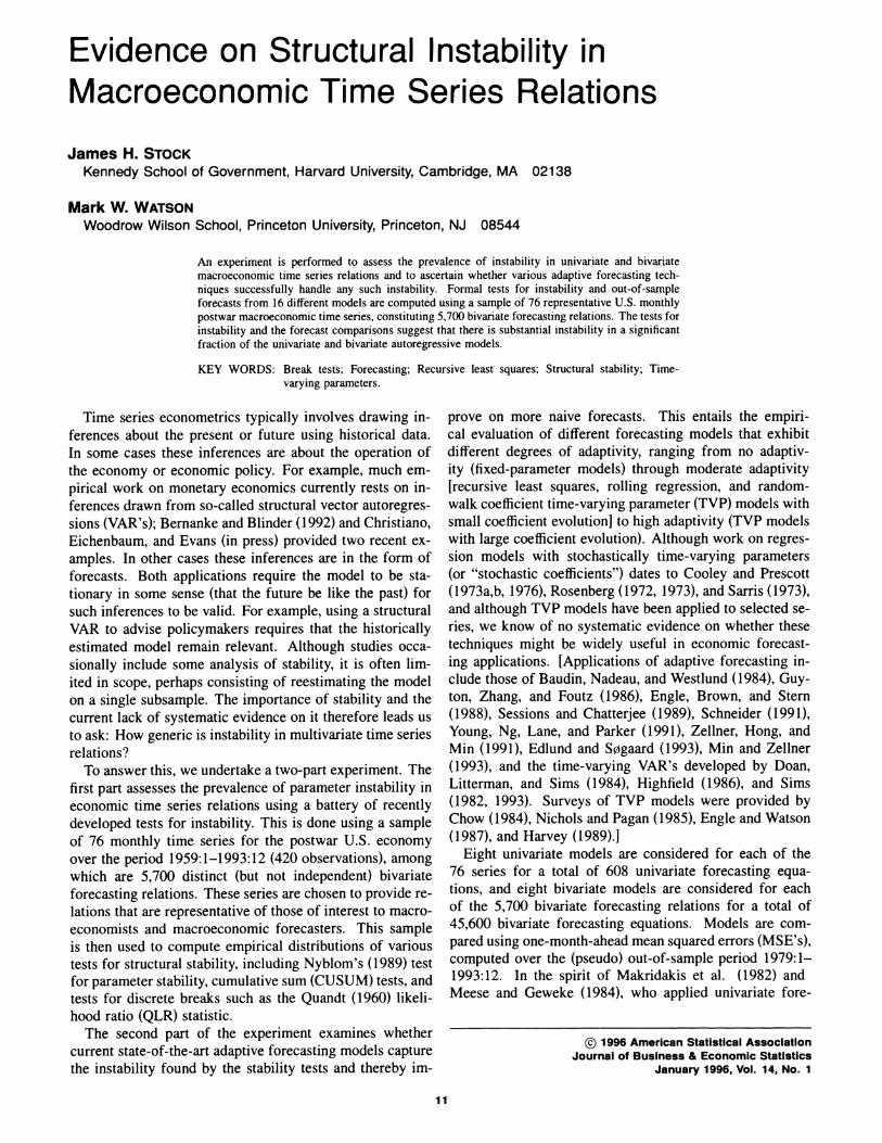
rameter stability with p = 6 are presented in Table 2 and Table B.2, Appendix B. The column labeled "GC" reports the Granger-causality Wald statistic testing the hypothesis that p(L) = 0 in (1). All tests have level 10%. The final three columns in Table B.2 summarize the distribution of estimated values of A, based on the QLR statistics.

Some of these tests indicate widespread instability. The QLR and EW statistics reject in over 55% of the cases. A large fraction (57%) of cases also have significant GC statistics, which is perhaps surprising because no a priori economic reasoning was used to select which variables should be used to forecast any particular dependent variable. As in the univariate results, the CUSUM-based tests have lower rejection rates, which suggests that the instability does not arise from breaks or drift in the direction of the mean regressors. There is only slightly more instability among statistically significant predictive relationships (based on the GC test) than among insignificant relationships.

These results can be used to examine stability in relations involving those variables that commonly appear in structural VAR modeling. QLR statistics for real personal income, the consumer price index, the producer price index, the 90-day Treasury-bill rate, and the commercial-paper- Treasury-bill spread each reject stability in at least 98% of their 75 respective bivariate relations when these series are used as dependent variables (Table B.2, Part I). When these series appear as predictor variables (Table B.2, Part II) for each the QLR rejects in at least 53% of the 75 pairs. For five of the seven price series, the QLR statistic rejects stability in each of the 75 bivariate forecasting relations in which inflation is a dependent variable. When any of these five price series is instead used as a predictor, the QLR statistic again rejects in approximately half the cases. It appears that instability in bivariate relations involving these key series is even more prevalent than on average across all 5,700 relations.

These marginal distributions provide one window on the extent of instability in these 5,700 relations. It is possible, however, that some of this instability is in relations that would be of little interest from a forecasting perspective because they have low overall predictive content. Explor- ing this possibility requires examining the joint distribution of the instability and GC test statistics. This is done graphically in Figure 1, a scatterplot of the QLR versus GC statistics. Evidently the QLR and GC test statistics are only weakly related. Similar low correlations are found between the other stability test statistics and the GC statistic. In a sense, each forecasting relation can be thought of as having a temporal average level of predictive content, and devi-


0d

O

o

o

01

o 1964 1968 1972 1976 1980 1984 1988

Year

Figure 2. Histogram of Break Dates From QLR Statistic.

ations from that predictive relation over time are largely uncorrelated with the average predictive content.

For these data, the QLR and the EW statistics have a cor- relation of .996 and produce similar inferences. Although they differ in theory, evidently little is lost in practice by considering only one or the other of these statistics.

Figure 2 summarizes the estimated break dates ([T6], where 6 maximizes FT(6)) for the bivariate relations for which the corresponding QLR statistics are significant at the 5% level. Instability is concentrated around 1974-1975, 1980-1981, and at the endpoints [6o and 61 in (7)]. 5.3 Sensitivity Analysis

The results in Tables 1 and 2 use fixed lag length p = 6, asymptotic critical values, and conventional forms of the test statistics. The sensitivity to these assumptions is explored in Table 3. Results for the univariate tests are reported in panel A. For comparison purposes, the first line repeats the base-case results from the first line of Table 1. For the second and third lines, the lag lengths were chosen by full-sample Akaike information criterion (AIC) and BIC, respectively, under the null hypothesis. For the fourth line, the asymptotic critical values were replaced by Monte Carlo critical values computed in the experiment

described in Section 2.4, with p = 6. In the final line, heteroscedasticity-robust versions of the test statistics were computed for p = 6 and evaluated using the Monte Carlo critical values for the heteroscedasticity-robust tests. Par- allel results are reported in panel B for the bivariate tests.

The sensitivity results are similar for both univariate and bivariate tests. Rejection rates drop somewhat using the Monte Carlo critical values, but the qualitative results in Tables 1 and 2 are robust to changes in lag selection and to the use of Monte Carlo critical values. The fraction of rejections by the QLR' and EW' statistic, however, is evidently much less than for their nonrobust counterparts: The bivariate QLR', MW', and EW' statistics indicate rejections of approximately 20% at the 10% level.

One interpretation of these results is that the heteroscedasticity-robust tests have less power than their nonrobust counterparts; another interpretation is that there is in fact considerable heteroscedasticity and the nonrobust tests are spuriously rejecting in many cases. Results from the Monte Carlo simulation described in Section 2.4 indicate that the nonrobust tests in Tables 1 and 2 have somewhat better power than those in Table 3 against the TVP alternative. For example, for A = .005 and .01, the 10% QLR test (using asymptotic critical values, as in Tables 1 and 2), respectively, has power 39% and 79%, but the QLR' test (using finite-sample critical values as in Table 3) has power 33% and 71%, respectively. This power difference seems insufficient, however, to be the sole explanation of the difference in empirical rejection rates. It thus appears that some of the rejections in Tables 1 and 2 arise from heteroscedasticity: Tables 1 and 2 arguably overstate instability because they are not robust, but the final line of Table 3 potentially understates instability because of lower power.

6. FORECASTING MODEL COMPARISON: EMPIRICAL RESULTS

The forecasting models described in Section 3.1 con- stitute 608 univariate forecasting systems (76 variables, eight models each) and 45,600 bivariate forecasting systems (5,700 bivariate forecasting relations, eight models each): All comparisons are made using out-of-sample one-month- ahead forecast MSE's, although in principle other loss func-

Table 3. Sensitivity Analysis for Stability Tests

Lag choice Critical values Hetero-robust? L PKsup PKmsq BP QLR MW EW

A. Univariate tests Fixed Asy. No 26.3 21.1 11.8 69.7 52.6 34.2 50.0 AIC Asy. No 23.7 17.1 10.5 76.3 57.9 32.9 53.9 BIC Asy. No 30.3 27.6 18.4 69.7 60.5 38.2 52.6 Fixed MC No 28.9 22.4 11.8 71.1 51.3 30.3 47.4 Fixed MC Yes 10.5 - - - 19.7 17.1 18.4

B. Bivariate tests Fixed Asy. No 17.5 18.7 15.4 66.5 57.7 35.0 56.2 AIC Asy. No 18.1 17.4 14.5 66.3 59.7 37.5 57.6 BIC Asy. No 30.9 26.8 24.1 66.9 60.2 43.6 55.6 Fixed MC No 27.5 21.5 15.9 67.7 52.7 32.0 50.8 Fixed MC Yes 14.2 - - - 19.5 20.1 19.2

NOTE: Percent of tests significant at 10% level.


Table 4. Best Out-of-Sample Forecasting Models: Percentage of Cases in Which Model Was Best Out-of-Sample

AR RRA 1 RRA2 RLSA ATVP1 ATVP2 ATVP3 ATVP4 VAR RRV1 RRV2 RLSV VTVP1 VTVP2 VTVP3 VTVP4

A. Summary

All models 19 3 0 8 7 3 6 7 12 3 3 6 8 5 3 6 10 BIC sel. 14 4 0 6 5 2 3 5 15 4 4 7 10 8 4 7 Stab. rej. 23 2 0 5 4 3 7 6, 15 4 4 6 6 6 4 5

B. Best models among all bivariate pairs, by variable being forecasted

A. Output and sales

ip 0 0 0 0 0 51 0 0 4 0 0 4 32 3 0 7

ipxmca 0 0 0 0 0 0 43 0 1 1 24 3 7 11 0 11

gmpy 58 0 0 0 0 0 0 0 38 0 0 0 1 2 0 2

gmyxp8 0 0 0 33 0 0 0 0 5 1 1 43 13 0 3 0

rtql 0 0 0 0 0 0 0 75 4 0 0 1 7 1 1 11

gmcq 0 0 0 0 0 0 73 0 0 1 3 1 3 13 3 3

ipcd 45 0 0 0 0 0 0 0 25 0 1 4 9 3 0 12 ced87m 0 0 0 0 0 76 0 0 0 0 7 1 1 13 0 1 xci 0 0 0 0 68 0 0 0 1 1 0 4 8 3 0 15 mt82 0 0 0 0 60 0 0 0 5 0 0 1 19 1 1 12

B. Employment Ipmhuadj 0 0 0 0 0 0 0 66 0 3 1 3 12 7 0 9

Iphrm 0 0 0 0 0 42 0 0 3 0 16 0 13 13 0 13 Ihel 0 0 0 0 0 0 47 0 3 0 3 13 9 19 5 1

Ihnaps 46 0 0 0 0 0 0 0 27 5 1 0 6 6 1 6 luinc 58 0 0 0 0 0 0 0 29 1 3 5 3 0 0 1 lhu5 0 0 0 48 0 0 0 0 7 0 0 9 27 3 0 7 Ihur 65 0 0 0 0 0 0 0 3 0 3 8 8 6 1 6 Ihelx 0 0 0 0 0 0 32 32 2 0 3 5 3 9 6 8

C. New orders

hsbp 0 21 0 0 0 0 0 0 43 11 5 9 4 1 0 5 mdu82 0 0 0 0 67 0 0 0 0 0 0 0 17 8 5 3 mpcon8 0 0 0 0 0 0 0 52 12 0 0 3 7 4 0 23 mocm82 0 0 0 0 0 0 37 0 7 1 0 1 27 7 8 12 mdo82 0 0 0 0 45 0 0 0 0 0 1 5 21 7 5 15 ivpac 0 43 0 0 0 0 0 0 8 9 8 20 0 1 5 5 pmi 0 0 0 0 0 0 0 69 4 0 4 4 4 1 1 12 pmno 0 0 0 13 0 0 0 0 10 1 12 31 8 1 0 23

D. Inventories invmt87 0 0 0 0 57 0 0 0 0 0 5 4 23 5 1 4 invrd 0 0 0 21 0 0 0 0 16 0 0 34 22 2 0 5 invwd 0 0 0 79 0 0 0 0 3 1 0 1 11 4 1 0 ivmld8 0 0 0 0 0 0 53 0 0 5 0 0 5 15 16 5 ivm2d8 0 0 0 0 67 0 0 0 1 0 1 1 21 5 1 1 ivm3d8 0 25 0 0 0 0 0 0 1 53 0 8 3 9 0 0 ivmtd 0 0 0 0 38 0 0 0 3 0 0 3 47 5 1 4 ivmld 0 0 0 0 0 0 39 0 0 9 0 0 7 36 8 1 ivm2d 0 0 0 0 0 0 0 55 1 0 0 1 22 3 1 16 ivm3d 0 0 0 0 0 44 0 0 0 1 1 3 20 29 1 0 invrd8 51 0 0 0 0 0 0 0 14 0 0 1 22 7 0 5 invwd8 0 0 0 0 59 0 0 0 0 0 0 1 31 0 0 9

E. Prices

gmdc 0 0 0 0 0 0 0 49 0 0 0 1 3 9 3 36 punew 0 0 0 0 0 0 0 80 0 0 0 0 0 4 5 11 pw 0 0 0 0 0 0 0 77 0 0 0 0 0 1 1 20 pw561 42 0 0 0 0 0 0 0 58 0 0 0 0 0 0 0

pw561r 0 0 0 0 4 0 0 0 5 0 7 68 16 0 0 0

jocci 0 0 0 53 0 0 0 0 6 1 0 24 7 6 0 2 joccir 50 0 0 0 0 0 0 0 35 0 1 0 4 1 1 9

F Interest rates

fyff 55 0 0 0 0 0 0 0 38 0 0 1 5 0 1 0

fygm3 57 0 0 0 0 0 0 0 41 0 0 1 0 0 1 0 fygm6 55 0 0 0 0 0 0 0 44 0 0 0 0 0 0 1 fygtl 49 0 0 0 0 0 0 0 40 0 1 2 4 0 0 3 fybaac 55 0 0 0 0 0 0 0 34 1 1 5 2 1 0 0

fygtlO 71 0 0 0 0 0 0 0 28 0 0 1 0 0 0 0

cp6_gm6 80 0 0 0 0 0 0 0 10 0 0 0 0 0 1 9

g10_gl 68 0 0 0 0 0 0 0 32 0 0 0 0 0 0 0


Table 4. (continued)

AR RRA1 RRA2 RLSA ATVP1 ATVP2 ATVP3 ATVP4 VAR RRVI RRV2 RLSV VTVP1 VTVP2 VTVP3 VTVP4

F Continued

gl0_ff 69 0 0 0 0 0 0 0 13 0 3 1 1 1 0 12 baa_g10 79 0 0 0 0 0 0 0 5 0 4 0 1 0 0 11

G. Money and credit

fcbuc 0 0 0 0 43 0 0 0 11 1 0 9 14 8 1 12 fcbcucy 0 0 0 0 0 59 0 0 0 0 0 0 9 17 8 7 delinqcr 0 0 0 0 36 0 0 0 0 5 3 13 19 5 0 19 cci30m 42 0 0 0 0 0 0 0 38 0 6 3 10 0 0 2 fmld82 0 0 0 0 0 5 0 0 1 40 1 7 1 19 21 4 fm2d82 0 33 0 0 0 0 0 0 0 45 0 4 0 7 9 1 fmbase 0 23 0 0 0 0 0 0 1 11 1 7 16 17 21 1 fml 0 0 0 53 0 0 0 0 1 1 0 7 7 24 5 1 fm2 0 0 0 0 0 0 53 0 0 0 0 1 3 11 29 3 fm3 0 0 0 0 0 0 57 0 0 0 0 0 1 5 24 12 fmbaser 0 0 0 0 0 0 37 0 0 1 1 1 3 13 35 8

H. Other variables

exnwt2 60 0 0 0 0 0 0 0 37 0 0 1 1 0 0 2 fspcomr 0 0 0 56 9 0 0 0 8 1 0 27 3 0 1 4 fspcom 0 0 0 57 0 0 0 0 4 0 0 28 2 0 1 8 fail 99 0 0 0 0 0 0 0 0 0 0 0 0 0 0 1 failr 99 0 0 0 0 0 0 0 0 0 0 0 0 0 0 1 gfosa 0 0 0 0 73 0 0 0 0 0 0 0 21 3 0 3 gfrsa 0 0 0 100 0 0 0 0 0 0 0 0 0 0 0 0 gfor 0 77 0 0 0 0 0 0 0 0 0 0 15 3 0 5 gfrr 0 0 0 96 0 0 0 0 0 0 3 1 0 0 0 0 hhsntn 0 0 15 0 0 0 0 0 0 7 79 0 0 0 0 0

C. Best models among those bivariate pairs with the 10 lowest in-sample BIC, by variable being forecasted

A. Output and sales

ip 0 0 0 0 0 50 0 0 20 0 0 0 30 0 0 0 ipxmca 0 0 0 0 0 0 30 0 0 0 30 0 10 0 0 30 gmpy 44 0 0 0 0 0 0 0 44 0 0 0 6 0 0 6 gmyxp8 0 0 0 20 0 0 0 0 30 0 0 50 0 0 0 0 rtql 0 0 0 0 0 0 0 40 30 0 0 10 10 0 0 10 gmcq 0 0 0 0 0 0 50 0 0 0 20 10 0 20 0 0 ipcd 20 0 0 0 0 0 0 0 40 0 0 30 10 0 0 0 ced87m 0 0 0 0 0 60 0 0 0 0 20 10 0 10 0 0 xci 0 0 0 0 60 0 0 0 0 0 0 30 0 0 0 10 mt82 0 0 0 0 40 0 0 0 20 0 0 0 20 0 0 20

B. Employment Ipmhuadj 0 0 0 0 0 0 0 10 0 20 0 20 30 10 0 10 Iphrm 0 0 0 0 0 0 0 0 0 0 10 0 60 30 0 0 Ihel 0 0 0 0 0 0 40 0 20 0 0 10 0 20 0 10 Ihnaps 10 0 0 0 0 0 0 0 20 30 0 0 0 20 10 10 luinc 40 0 0 0 0 0 0 0 50 10 0 0 0 0 0 0 Ihu5 0 0 0 20 0 0 0 0 30 0 0 20 30 0 0 0 Ihur 18 0 0 0 0 0 0 0 0 0 0 18 18 18 9 18 Ihelx 0 0 0 0 0 0 15 15 8 0 0 0 8 31 8 15

C. New orders

hsbp 0 70 0 0 0 0 0 0 0 10 0 10 0 10 0 0 mdu82 0 0 0 0 50 0 0 0 0 0 0 0 10 20 10 10 mpcon8 0 0 0 0 0 0 0 30 0 0 0 20 20 0 0 30 mocm82 0 0 0 0 0 0 10 0 40 0 0 0 30 10 0 10 mdo82 0 0 0 0 20 0 0 0 0 0 0 10 50 0 0 20 ivpac 0 30 0 0 0 0 0 0 0 30 0 0 0 10 20 10 pmi 0 0 0 0 0 0 0 60 10 0 10 10 0 0 0 10 pmno 0 0 0 0 0 0 0 0 40 0 20 20 0 10 0 10

0. Inventories

invmt87 0 0 0 0 0 0 0 0 0 0 20 10 30 20 10 10 invrd 0 0 0 20 0 0 0 0 40 0 0 20 0 20 0 0 invwd 0 0 0 50 0 0 0 0 0 0 0 10 20 20 0 0 ivmld8 0 0 0 0 0 0 10 0 0 10 0 0 10 30 10 30 ivm2d8 0 0 0 0 50 0 0 0 0 0 10 0 30 0 10 0 ivm3d8 0 40 0 0 0 0 0 0 0 30 0 10 0 20 0 0 ivmtd 0 0 0 0 0 0 0 0 17 0 0 8 42 8 0 25


Table 4. (continued)

AR RRA 1 RRA2 RLSA ATVP1 ATVP2 ATVP3 ATVP4 VAR RRV1 RRV2 RLSV VTVP1 VTVP2 VTVP3 VTVP4

D. Continued

ivmld 0 0 0 0 0 0 0 0 0 0 0 0 0 100 0 0 ivm2d 0 0 0 0 0 0 0 18 0 0 0 0 55 9 0 18 ivm3d 0 0 0 0 0 10 0 0 0 10 10 10 40 20 0 0 invrd8 40 0 0 0 0 0 0 0 10 0 0 0 40 0 0 10 invwd8 0 0 0 0 50 0 0 0 0 0 0 10 10 0 0 30

E. Prices

gmdc 0 0 0 0 0 0 0 60 0 0 0 0 0 0 0 40

punew 0 0 0 0 0 0 0 90 0 0 0 0 0 0 0 10

pw 0 0 0 0 0 0 0 70 0 0 0 0 0 0 0 30

pw561 60 0 0 0 0 0 0 0 40 0 0 0 0 0 0 0

pw561r 0 0 0 0 0 0 0 0 40 0 0 60 0 0 0 0

jocci 0 0 0 40 0 0 0 0 50 0 0 10 0 0 0 0

joccir 40 0 0 0 0 0 0 0 60 0 0 0 0 0 0 0

F Interest rates

fyff 50 0 0 0 0 0 0 0 40 0 0 0 10 0 0 0

fygm3 20 0 0 0 0 0 0 0 60 0 0 10 0 0 10 0

fygm6 30 0 0 0 0 0 0 0 60 0 0 0 0 0 0 10

fygtl 20 0 0 0 0 0 0 0 70 0 0 0 0 0 0 10

fybaac 40 0 0 0 0 0 0 0 40 0 0 10 10 0 0 0

fygtl 0 60 0 0 0 0 0 0 0 30 0 0 10 0 0 0 0

cp6_gm6 80 0 0 0 0 0 0 0 0 0 0 0 0 0 10 10

glO_gl 90 0 0 0 0 0 0 0 10 0 0 0 0 0 0 0

g10_ff 40 0 0 0 0 0 0 0 30 0 10 0 0 10 0 10

baa_g10 60 0 0 0 0 0 0 0 10 0 20 0 0 0 0 10

G. Money and credit

fcbcuc 0 0 0 0 10 0 0 0 20 0 0 20 40 10 0 0

fcbcucy 0 0 0 0 0 0 0 0 0 0 0 0 30 60 0 10

delinqcr 0 0 0 0 40 0 0 0 0 10 20 0 10 0 0 20

cci30m 50 0 0 0 0 0 0 0 10 0 40 0 0 0 0 0

fmld82 0 0 0 0 0 10 0 0 0 50 0 0 0 20 20 0

fm2d82 0 40 0 0 0 0 0 0 0 50 0 0 0 10 0 0

fmbase 0 42 0 0 0 0 0 0 0 33 8 0 8 0 8 0

fml 0 0 0 60 0 0 0 0 0 10 0 0 10 20 0 0

fm2 0 0 0 0 0 0 10 0 0 0 0 10 0 20 50 10

fm3 0 0 0 0 0 0 40 0 0 0 0 0 0 0 50 10

fmbaser 0 0 0 0 0 0 20 0 0 10 0 0 0 10 50 10

H. Other variables

exnwt2 80 0 0 0 0 0 0 0 20 0 0 0 0 0 0 0

fspcomr 0 0 0 40 0 0 0 0 30 0 0 30 0 0 0 0

fspcom 0 0 0 40 0 0 0 0 20 0 0 40 0 0 0 0

fail 100 0 0 0 0 0 0 0 0 0 0 0 0 0 0 0

failr 100 0 0 0 0 0 0 0 0 0 0 0 0 0 0 0

gfosa 0 0 0 0 100 0 0 0 0 0 0 0 0 0 0 0

gfrsa 0 0 0 100 0 0 0 0 0 0 0 0 0 0 0 0

gfor 0 100 0 0 0 0 0 0 0 0 0 0 0 0 0 0

gfrr 0 0 0 80 0 0 0 0 0 0 20 0 0 0 0 0

hhsntn 0 0 30 0 0 0 0 0 0 10 60 0 0 0 0 0

NOTE: See Appendix A for series descriptions. The first row of panel A shows results for all 76 x 76 models. Entries in the second row are the corresponding fraction, except that the set of bivariate relations is restricted from 75 to 10 for each forecasted variable, where the 10 predictors are chosen to be those with the lowest in-sample BIC for the forecasted variable at hand. Entries in the third row are for the set of bivariate relations restricted to be those for which the QLR statistic is significant at the 10% level, when calculated through 1978:12. Panel B shows detailed results for all models for each variable, and panel C shows detailed results for the 10 best fitting (in-sample) models for each variable. When two or more models were tied as the best performer (to eight significant digits), then each was counted as best. The in-sample period was from the later of 1959:1 or the first data for which data are available, to 1978:12, and the out-of-sample period is from 1979:1 through the earlier of the final date for the series or 1993:12.

tions could be used. The term "best model" refers to the model that minimizes this out-of-sample forecast MSE, relative to some comparison group. One objective of this comparison is to see which models do best most frequently. Be- cause of the instability found by the stability tests, however, another objective is to ascertain which if any of the models

protect the forecaster from making extreme forecast errors

resulting from parameter instability. The question of which model performs best out-of-

sample most frequently is examined in Table 4. For each bivariate relation, MSE's from the eight bivariate and eight univariate models were computed; the model with the lowest out-of-sample MSE among these 16 was then deemed the "best" model for that (yt, xt) pair. Two sets of tab-


Table 5. Comparison of Out-of-Sample Forecasts Among all 5,700 Bivariate Bivariate Combinations

Model AR RRA1 RRA2 RLSA ATVP1 ATVP2 ATVP3 ATVP4 VAR RRV1 RRV2 RLSV VTVP1 VTVP2 VTVP3 VTVP4

AR - 63 55 36 42 43 51 45 48 62 53 45 44 49 59 46 RRA1 37 - 38 26 25 24 49 33 45 59 42 32 34 43 58 38 RRA2 45 62 - 21 28 38 57 39 54 65 49 41 40 49 63 45 RLSA 64 74 79 - 41 55 66 45 64 72 63 51 51 57 70 52 ATVP1 58 75 72 59 - 66 71 63 64 74 66 58 58 66 75 59 ATVP2 57 76 62 45 34 - 74 54 60 68 59 50 49 61 73 51 ATVP3 49 51 43 34 29 26 - 36 53 58 50 39 36 45 67 40 ATVP4 55 67 61 55 37 46 63 - 60 68 58 52 50 57 71 54

VAR 28 55 46 36 36 40 47 40 - 57 47 33 36 44 56 38 RRV1 38 38 35 28 26 32 42 32 43 - 30 22 27 36 53 31 RRV2 47 58 47 37 34 41 50 42 53 70 - 27 36 46 64 41 RLSV 55 68 59 42 42 50 61 48 67 78 73 - 46 57 71 50 VTVP1 56 66 60 49 42 51 64 50 64 73 64 54 - 69 78 55 VTVP2 51 57 51 43 34 39 55 43 56 64 54 43 31 - 82 45 VTVP3 41 42 37 30 25 27 33 29 44 47 36 29 22 18 - 26 VTVP4 54 62 55 48 41 49 60 46 62 69 59 50 44 55 74 -

NOTE: Entries are the percentage of times that row forecast MSE is less than column forecast MSE. See the notes to Table 4.

ulations are presented. Panel B presents the fraction of times the column model is best among the 75 bivariate relations, broken down by forecasted variable. For example, for industrial production, in 51% of the 75 bivariate pairs, ATVP2 produces the smallest out-of-sample MSE, and in 32% of the pairs, VTVP1 performs best. Panel C presents analogous results, broken down by forecasted variable, except that for each forecasted variable the comparison is only among the top 10 of the 75 pairs, as measured by the BIC for the in-sample OLS estimation of (1) with fixed parameters. Thus, among forecasts of industrial production based on the 10 variables with the lowest in-sample BIC's, in two cases (20%) VAR has the lowest out-of-sample MSE, but in five cases ATVP2 performs best. The first two rows of panel A, respectively, summarize the results of panels B and C, in which the fractions are computed over all the forecasted variables. The final row of panel A presents results for bivariate relations with significant time variation, as measured by significance (at the 10% level) of the QLR statistic evaluated for the in-sample period.

Several conclusions are evident from Table 4. Overall, there is no clearly dominant model. There is strong evidence, however, that the adaptive models (the rolling and TVP models) often outperform the fixed-parameter models. Comparing the final row of panel A with the first two

Table 6. Selected Quantiles of Distributions of Mean Squared Forecast Errors Relative to MSE for the AR Recursive

Least Squares (RLSA) Forecast: Univariate Forecasts

Percentile

Model Min .050 .250 .500 .750 .950 Max

AR .905 .959 .994 1.003 1.017 1.060 1.346 RRA1 .956 .972 .999 1.012 1.027 1.060 1.066 RRA2 .958 .982 1.001 1.004 1.011 1.045 1.069 ATVP1 .911 .979 .991 .999 1.003 1.026 1.060 ATVP2 .948 .969 .993 1.002 1.007 1.055 1.073 ATVP3 .936 .968 .993 1.009 1.022 1.097 1.142 ATVP4 .929 .961 .989 .999 1.008 1.051 1.091

NOTE: Mean squared forecast errors are relative to mean squared error of the recursive least squares AR forecast.

rows indicates that the adaptive models perform similarly whether or not in-sample instability is detected. Although the ATVP and VTVP models as a group often perform best, among TVP models the estimation of A by PLS is arguably worse than fixing it at some small value. Consistent with the stability test evidence, the results in panels B and C show that different variables tend to be forecast best by different models.

Table 5 summarizes pairwise comparisons of these 16 models over all 5,700 bivariate relations. Among univariate models, ATVP1 performs best most often, and RLSA is on average outperformed only by ATVP1. Among bivariate models, VTVP1 performs best most often. In both the univariate and bivariate cases, estimation of A (ATVP4 and VTVP4) worsens performance, relative to using the fixed value A = .0025, in a majority of cases. Although the ATVP1 model typically outperforms the bivariate models, this is perhaps not surprising because a priori reasoning would lead one to suspect that many of the 5,700 pairs would have forecasting links that are weak at best.

In addition to the models reported in Tables 4 and 5, 48 fixed-lag versions of these models and 12 other TVP models (A = .005, .01, .02; p = 1, 3, 6, and PLS) were estimated (detailed results are available from the authors on request). In general, the models with data-dependent lag lengths outperform the fixed-lag models. Moreover, models with large time variation (A = .02) do poorly.

Tables 6, 7, and 8 examine the extent to which the various models reduce the possibility of extremely poor performance by presenting empirical quantiles of the MSE's of the various models. To make results comparable across series, the MSE's are relative to the MSE for RLSA. The distribution of these relative MSE's is given in Table 6 for univariate forecasting models and in Table 7 for the bivariate models. The median values are less than 1 for ATVP1 and ATVP4, the models that outperform RLSA in the pairwise comparisons in Table 5. The results in Table 6 indicate that the costs of using the ATVP1 model, as measured by its worst performance relative to RLSA, are small, but in the best case the MSE forecasting gains of ATVP1 relative to RLSA are 9%. The risks of using fixed-parameter


Table 7. Selected Quantiles of Distributions of Mean Squared Forecast Errors Relative to MSE for the AR Recursive Least Squares (RLSA) Forecast: Bivariate Forecasts (all)

Percentile

Model Min .001 .005 .010 .050 .250 .500 .750 .950 .990 .995 .999 Max

VAR .500 .620 .899 .905 .951 .993 1.008 1.032 1.125 1.190 1.256 1.345 2.249 RRV1 .477 .597 .915 .930 .959 .997 1.011 1.034 1.073 1.130 1.137 1.148 1.168 RRV2 .477 .597 .908 .920 .949 .993 1.005 1.022 1.058 1.115 1.121 1.137 2.003 RLSV .473 .591 .901 .916 .948 .990 1.000 1.013 1.042 1.105 1.116 1.124 1.135 VTVP1 .478 .596 .895 .908 .944 .986 1.001 1.014 1.050 1.096 1.110 1.151 1.200 VTVP2 .489 .593 .901 .913 .949 .987 1.005 1.023 1.075 1.120 1.141 1.170 1.259 VTVP3 .490 .606 .906 .921 .955 .994 1.015 1.041 1.115 1.175 1.196 1.258 1.391 VTVP4 .476 .592 .901 .916 .945 .984 1.001 1.016 1.067 1.122 1.143 1.224 1.306


models are clear: In 1% of the relations the MSE of the fixed-parameter VAR is 19% more than that of RLSA. One measure of model robustness is obtained by comparing the relative MSE at the ath quantile to the inverse of the relative MSE at the (1 - a)'th quantile. For example, the relative MSE of VTVP4 at a = .001 is .592 so that in .1% of the casts VTVP4 outperforms RLSA by at least 40%. At a = .999, the relative MSE of VTVP4 is 1.224 so that in .1% of the cases RLSA outperforms VTVP4 by more than 18%. In this sense, in the .1% extremes, VTVP4 produces better forecasts than RLSA. By this measure, at the .1% quantile, all the bivariate models dominate RLSA, and at a = .5% and 1%, all the bivariate TVP models dominate RLSA. If attention is restricted to those models with the best 10 in-sample predictors (Table 8), the improvements in the left tail in the bivariate TVP models is even more dramatic: Not surprisingly, presample predictor selection improves out-of-sample performance.

Although the TVP models guard against large parameter shifts, it should be emphasized that the gains from using TVP models are generally small or nonexistent. For example, RLSV, which is efficient under constant parameters, has approximately the same quantiles as VTVP1 and VTVP2 and indeed outperforms all bivariate models but VTVP1 in pairwise comparisons.

Empirical distributions of the estimates of A are summa- rized in Table 9, computed as discussed in Section 4.1. For comparison purposes, the final three rows in each panel re- port Monte Carlo null distributions of the PLS estimator of A and of the median-unbiased estimators of A based on the

QLR and QLRr statistics, produced by inverting the Monte Carlo QLR statistics generated under A = 0. The distributions of the three empirical estimates have some similarities. Many of the relations are well described by constant parameter models, but this number is less than implied by the null Monte Carlo distributions. There is also evidence that some of the systems also exhibit substantial time variation. For example, among the bivariate relations, A is estimated to be at least .01 in 65% of the systems using the QLR estimator in 36% using the QLRr estimator, but under the null approximately 20% of the QLR and QLRr estimates would exceed .01.

Table 10 reports estimates of the distribution of A computed as discussed in Section 4.2. The point estimates of the distributions differ across procedures, with the QLR having the largest estimates of mass at high values of A and the QLRr having the lowest. Based on the PLS estimates, approximately 23% of the mass is estimated to fall on A > .01 for both the univariate and bivariate relations. The distribution estimated using the QLR and QLRr statistics indicates a substantial amount of moderate time variation (0 < A < .01). In all three distributions in the bivariate case, at least one-fifth of the mass is placed on A>2 .0075.

7. DISCUSSION AND CONCLUSIONS

Although these tests focus on univariate and bivariate linear models, the low-dimensionality and linearity are not re- strictive. If the parameters of a higher-dimensional VAR are constant, then the parameters of all possible bivariate VAR's formed from variables in the higher-dimensional VAR will

Table 8. Selected Quantiles of Distributions of Mean Squared Forecast Errors Relative to MSE for the AR Recursive Least Squares (RLSA) Forecast: Best 10 Bivariate Models as Selected Using In-sample BIC

Percentile

Model Min .005 .010 .050 .250 .500 .750 .950 .990 .995 Max

VAR .500 .670 .897 .929 .973 1.001 1.036 1.158 1.308 1.332 1.466 RRV1 .477 .676 .909 .937 .981 1.004 1.023 1.066 1.137 1.142 1.168 RRV2 .477 .655 .895 .930 .974 .997 1.015 1.059 1.128 1.135 1.142 RLSV .473 .664 .886 .925 .971 .992 1.009 1.045 1.120 1.132 1.135 VTVP1 .478 .652 .889 .921 .966 .993 1.012 1.045 1.108 1.117 1.131 VTVP2 .489 .663 .887 .924 .971 .997 1.019 1.067 1.123 1.141 1.170 VTVP3 .490 .674 .894 .932 .977 1.007 1.036 1.107 1.185 1.228 1.391 VTVP4 .476 .653 .885 ,921 .966 .991 1.013 1.071 1.144 1.177 1.259



Table 9. Distribution of Estimates of A

Distribution 0 .0025 .0050 .0075 .0100 .0150 .0200

A. Univariate models PLS 55.3 5.3 3.9 10.5 11.8 5.3 7.9 QLR 22.4 10.5 1.3 7.9 11.8 15.8 30.3 QLRr 46.1 6.6 10.5 5.3 17.1 9.2 5.3

PLS (A = 0) 65.5 10.6 10.5 6.2 4.7 1.4 1.1 QLR (A = 0) 55.0 5.7 9.3 9.8 12.7 5.8 1.7 QLR' ( = 0) 55.6 5.0 8.5 11.0 11.4 6.8 1.6

B. Bivariate models PLS 55.1 10.0 9.4 8.4 6.3 3.6 7.2 QLR 20.9 2.2 3.9 8.1 16.2 18.8 29.8 QLR' 42.7 4.3 7.9 9.7 16.9 11.8 6.8

PLS (A = 0) 66.1 11.8 11.6 6.3 2.2 1.2 0.8 QLR (A = 0) 56.9 5.2 7.3 10.4 12.5 6.5 1.3 QLR' (A = 0) 55.8 5.4 7.5 9.8 12.0 7.4 2.1

NOTE: Entries are the percentages of estimates of A based on the procedure indicated in the first column that take on the value in the row heads (for the PLS estimates) or which fall in a bin around the row value (for the QLR and QLRr estimates). The distributions with x = 0 are simulated null distributions. The estimators are described in the text.

be stable. Thus instability in one of these bivariate VARs implies instability in the higher-dimensional VAR, so evidence of instability in bivariate systems can be extrapolated to implied instability in larger systems. Similarly, by focus- ing on linear systems this analysis examines the stability of linear projections or, equivalently in population, of Wold representations and second moments. Using a linear rep- resentation of a nonlinear model still permits examining the second-order stationarity of these systems, even though these linear VAR's will be misspecified and thus will not have structural interpretations (compare Hendry, Pagan, and Sargan 1984).

The empirical results suggests that a substantial fraction of forecasting relations are unstable. In most cases this instability is small enough that, at best, adaptive models only slightly outperform nonadaptive models. Some cases exhibit great instability, however, with large estimated A and with adaptive models outperforming nonadaptive ones by a considerable margin. A value of A = .01 implies that the standard deviation of the drift in coefficients on standard- ized regressors over samples of the length considered here is approximately .2, which is consistent with rather large changes in autoregressive coefficients.

The implications of these findings depends on the application at hand. If the application is VAR modeling, or econometric modeling more generally, this suggests that instability in VAR's could be commonplace, which in turn calls into question the relevance of policy implications drawn from fixed-parameter VAR's. One practical lesson that this emphasizes is the importance of performing systematic stability analysis as part of a structural VAR modeling exercise.

On the other hand, if the application is to forecasting, this instability provides an opportunity to improve on the forecasts of fixed-parameter models. Although the random- walk TVP models used here are a step in that direction, the gains in terms of one-quarter-ahead forecast MSE, rel-

Table 10. Estimates of the Distribution of A

Distribution 0 .0025 .0050 .0075 .0100 .0150 .0200

A. Univariate models PLS 75.3 .0 .0 .0 11.6 .0 13.1 QLR .0 .0 .0 55.5 .0 7.2 37.3 QLR' 32.6 .0 65.0 .1 .0 .0 2.4

B. Bivariate models PLS 77.7 .0 .0 .0 6.6 .0 15.7 QLR 2.3 .7 3.8 6.1 49.8 10.7 26.6 QLR' .0 36.3 .0 63.7 .0 .0 .0

NOTE: Entries are the percentage mass of the distribution of A that falls in the bin around the value in the row header, computed as the solution to the deconvolution problem described in Section 4.2.

ative to recursive least squares models, are usually small. When R2's are low, relatively large changes in coefficients can produce modest changes in forecast MSE's so that statistically significant parameter variation might be only marginally significant from a forecasting perspective. In addition, the gains from TVP models could be greater at longer horizons, an issue not explored in this research. Nonetheless, this finding raises the question of whether more tightly parameterized refinements of the TVP model, or other adaptive models, could perform better than the standard TVP model used here.

ACKNOWLEDGMENTS

We are grateful to Frank Diebold, Jan Eberly, Bruce Hansen, Andrew Harvey, Serena Ng, Neil Shephard, Ken- neth Wallis, and participants at the 14th Annual Interna- tional Symposium on Forecasting in Stockholm, Sweden, for helpful discussions and/or comments on an earlier draft. This research was supported by National Science Founda- tion Grants SES-91-22463 and SBR-9409629.

APPENDIX A: DEFINITIONS OF SERIES

The entries for each series are the series mnemonic, the transformation code, and the definition of the series. For series obtained from CITIBASE, the CITIBASE mnemonic has been used. The transformation codes are 0 = first difference, 1 = log first difference, 2 = level.

A. Output and Sales ip 1 index of industrial production; ipxmca 2 capacity util rate: manufacturing,total(% of capacity,sa)(frb); gmpy 1 personal income: total (bil$,saar); gmyxp8 1 personal income (real) less transfers; rtql 1 retail trade: total (mil.87$)(s.a.); gmcq 1 personal consumption expendi- ture:total (bi11.1987$); ipcd 1 industrial production: durable consumer gds (1987 = 100,sa); ced87m 1 personal consumption expenditures:durable goods,87$; xci I stock- watson index of coincident indicators; mt82 1 manuf. and trade sales

B. Employment

lpmhuadj 1 total employee hours (adjusted); lphrm 2 avg. weekly hrs. of production wkrs.: manufacturing (sa); lhell


1 index of help-wanted adv.; lhnaps 1 persons at work: part time eas-slack wk,nonag (thous,sa); luinc 2 avg wkly initial claims,state unemploy.ins.,exc p.rico(thous;sa); lhu5 1 unemploy.by duration: persons unempl.less than 5 wks (thous.,sa); lhur 0 unemployment rate: all workers, 16 years & over (%,sa); lhelx 2 employment: ratio; help-wanted ads:no. unemployed clf

C. New Orders hsbp 2 housing authorized: index of new priv housing units (1967 = 100; sa); mdu82 1 mfg unfilled orders: durable goods industries, 82$; mpcon8 1 contracts & orders for plant & equipment in 82$(bil$,sa) 2; mocm82 1 mfg new orders: consumer goods & material,82$(bil$,sa) 2; mdo82 1 mfg new orders: durable goods industries,82$(bil$,sa) 2; ivpac 2 vendor performance: % of co's reporting slower deliveries(%,nsa); pmi 2 purchasing managers' index (sa); pmno 2 napm new orders index (percent)

D. Inventories invmt87 1 manufacturing & trade inventories:total,87$ (bil$,sa) invrd 1 inventories, retail (sa); invwd 1 inventories, wholesale (sa); ivmld8 1 mfg inventories: materials & supplies, all mfg indus 87$(sa); ivm2d8 1 mfg inventories: work in process, all mfg indus 87$(sa); ivm3d8 1 mfg inventories: finished goods, all mfg industries 87$(sa); ivmtd 1 manufacturing & trade inventories:total; ivmld 1 mfg inventories: materials & supplies, all mfg indus (mil$,sa); ivm2d 1 mfg inventories: work in process, all mfg indus (mil$,sa); ivm3d 1 mfg inventories: finished goods, all mfg industries (mil$,sa); invrd8 1 inventories, retail 87$ (sa); in- vwd8 1 inventories, wholesale 87$ (sa)

E. Prices gmdc 1 pce,impl pr defl:pce (1987 = 100); punew 1 cpi- u: all items (82-84 = 100, sa); pw 1 producer price index: all commodities (82 = 100,nsa); pw561 1 producer price index: crude petroleum (82 = 100,nsa); pw56lr 1 pw561/punew; jocci 1 dept. of commerce commodity price index; joccir 1 jocci/punew

F Interest Rates fyff 0 interest rate: federal funds (effective) (% per annum,nsa); fygm3 0 interest rate: U.S. treasury bills,sec mkt,3-mo.(% per ann,nsa); fygm6 0 interest rate: U.S.treasury bills,sec mkt,6-mo.(% per ann,nsa); fygtl 0 interest rate: U.S.treasury const maturities, 1-yr.(% per ann,nsa); fybaac 0 bond yield: moody's baa corporate (% per annum); fygtl0 0 interest rate: U.S.treasury const maturities,10-yr.(% per ann,nsa); cp6_gm6 2 yield on 6 month commercial paper - fygm6; gl0_gl 2 fytl0 - fygtl; glO_ff 2 fygtl0 - fyff; baa_gl0 2 fybaac - fygtl0 G. Money and Credit fcbcuc 2 change in bus and consumer credit out- stand.(percent,saar)(bcd 111); fcbcucy 2 fcbcuc-annual percentage growth in GMPY; delinqcr 0 delinq. rate, total in- stall. credit; cci30m 0 consumer instal.loans: delinquency rate,30 days & over, (%,sa); fmld82 1 money stock: m-1 in 1982$ (bil$,sa)(bcd 105); fm2d82 1 money stock: m-2 in 1982$(bil$,sa)(bcd 106); fmbase 1 monetary base, adj for reserve req chgs(frb of st.louis)(bil$,sa); fml 1 money stock: ml(curr,trav.cks,dem dep,other ck'able dep)(bil$,sa); fm2 1 money stock:m2(ml + o'nite rps,euro$,g/p&b/d mmmfs&sav&sm time dep(bil$,; fm3 1 money stock: m3(m2 + ig time dep,term rp's&inst only mmmfs)(bil$,sa); fmbaser 1 monetary base: fmbase/punew H. Other Variables exnwt2 1 Trade weighted average nominal exchange rate; fspcom 1 s&p's common stock price index: composite (1941-43 = 10); fspcomr 1 fspcom/punew; fail 1 business failures: current liabilities (mil$,nsa); failr 1 fail/punew; gfosa 1 federal government outlays seasonally adjusted; gfrsa 1 federal government receipts seasonally adjusted; gfor 1 Real federal government outlays, gfosa/punew; gfrr 1 Real federal government receipts, gfrsa/punew; hhsntn 2 u. of mich. index of consumer expectations(bcd-83)

APPENDIX B: SUPPLEMENTARY TABLES

The following tables are supplementary to Tables 1 and 2.

Table B. 1. Univariate Tests for Stability-Results for Individual Series

Test

Series Sample L PKsup PKmsq BP QLR MW EW F A

A. Output and sales

ip 59:2 93:12 1.12 .62 .09 24.37*** 11.58 6.43 4.02 13.01*** .0000 ipxmca 59:1 93:12 1.08 .78 .13 34.35*** 10.92 6.43 3.80 2912.69*** .0000 gmpy 59:2 93:12 3.52*** 1.26* .44* 143.28*** 55.29*** 20.82*** 24.80*** 3.36*** .0250 gmyxp8 59:2 93:12 4.95*** .98 .23 133.61*** 66.26*** 27.47*** 30.08*** 4.67*** .0250 rtql 59:2 93:12 .96 .69 .05 43.27*** 16.94 6.61 5.19 4.64*** .0077 gmcq 59:2 93:12 1.80* 1.27* .41" 46.40*** 24.03** 12.04** 8.32** 2.48** .0155 ipcd 59:2 93:12 1.38 .60 .07 54.83*** 12.79 9.09 5.11 2.30** .0000 ced87m 59:2 93:10 3.11*** .64 .06 57.34*** 47.50*** 20.89*** 18.85*** 5.44*** .0250 xci 59:3 93:12 .93 .68 .11 36.56*** 18.06 6.19 4.98 21.63*** .0092 mt82 59:2 93:12 1.12 .66 .06 15.84** 12.31 7.16 4.31 2.60** .0000

B. Employment

Ipmhuadj 59:2 93:12 1.10 .51 .06 16.30** 15.38 7.07 4.94 8.27*** .0053


Table B.1. (continued)

Test

Series Sample L PKsup PKmsq BP QLR MW EW F

B. Continued

Iphrm 59:1 93:12 .94 1.26* .21 27.68*** 20.37* 5.67 4.87 315.83*** .0120 Ihel 59:2 93:12 1.90* .41 .04 15.37** 30.35*** 11.74** 11.62*** 18.92*** .0213 Ihnaps 59:2 93:12 1.46 .56 .05 32.70*** 14.01 9.47 5.38 3.25*** .0010 luinc 59:1 93:12 1.31 1.04 .24 55.83*** 21.15* 9.19 6.93* 1271.59*** .0125 Ihu5 59:2 93:12 1.06 .88 .15 10.98* 14.17 5.90 4.45 14.94*** .0023 Ihur 59:2 93:12 1.32 .78 .05 20.64*** 14.36 8.31 5.07 10.88*** .0027 Ihelx 59:1 93:12 1.21 .98 .21 63.83*** 30.34*** 8.94 9.90*** 6348.62*** .0213

C. New orders

hsbp 59:1 93:12 1.46 .65 .06 21.58"** 21.87** 10.90* 7.57* 995.43*** .0132 mdu82 59:2 93:12 2.13** .92 .26 2.19 23.12** 13.97*** 9.26** 56.67*** .0148 mpcon8 59:2 93:9 .62 .57 .06 24.97*** 11.46 4.44 2.89 17.18"** .0000 mocm82 59:2 93:9 1.14 .74 .11 12.82** 16.11 8.24 5.47 3.12*** .0065 mdo82 59:2 93:9 1.44 .73 .12 4.23 28.93*** 9.87 9.64** 7.37*** .0200 ivpac 59:1 93:12 1.32 .91 .13 15.41*' 22.25** 8.84 7.63* 682.87*** .0138 pmi 59:1 93:12 .99 .87 .15 7.17 12.46 6.20 3.90 515.96*** .0000 pmno 59:1 93:12 1.14 .63 .08 5.63 14.35 7.02 4.80 232.21** .0025

D. Inventories

invmt87 59:2 93:9 .93 .87 .21 4.28 12.35 5.57 3.67 22.57*** .0000 invrd 59:1 93:9 1.16 .78 .21 9.40 12.73 6.51 4.07 4.85*** .0000 invwd 59:1 93:9 1.80* 1.12 .23 25.81*** 21.88** 11.16* 8.14** 12.53*** .0132 ivmld8 59:2 93:9 1.62 1.13 .23 8.72 27.34*** 10.64* 9.10** 21.99*** .0187 ivm2d8 59:2 93:9 .82 .85 .21 6.93 11.20 4.74 3.24 26.51*** .0000 ivm3d8 59:2 93:9 1.62 1.21* .47** 3.17 19.52* 10.12* 6.35 7.99*** .0110 ivmtd 59:1 93:9 .85 1.07 .24 15.37** 13.39 5.87 3.78 74.88*** .0000 ivmld 59:1 93:9 1.74* 1.01 .19 32.67*** 23.90** 11.67** 8.17** 63.00*** .0155 ivm2d 59:1 93:9 .63 .93 .18 7.42 7.76 3.64 2.18 53.91*** .0000 ivm3d 59:1 93:9 1.45 1.42** .33 9.80 19.02 9.34 6.12 25.10*** .0105 invrd8 59:2 93:9 1.30 .65 .06 15.58** 14.07 7.69 5.13 5.51*** .0018 invwd8 59:2 93:9 1.77* .95 .15 24.01*** 20.24* 10.19* 7.65* 3.07*** .0118

E Prices

gmdc 59:2 93:12 1.49 .75 .17 4.26 40.06*** 13.99"** 15.72"** 42.14"** .0250 punew 59:2 93:12 2.34*** .74 .15 18.22*** 43.01*** 19.39"** 17.58*** 74.09*** .0250 pw 59:2 93:12 2.35*** .97 .23 112.10"** 93.17"** 19.72"** 40.93*** 17.20"** .0250 pw561 59:2 93:12 2.22** 1.28* .29 53.95*** 55.43*** 13.07** 23.73*** 10.90*** .0250 pw561r 59:2 93:12 1.91"* 1.16 .23 46.35*** 48.36*** 10.60* 20.04*** 10.11*** .0250 jocci 59:2 93:11 1.11 .60 .08 22.11*** 25.98** 7.22 9.28** 21.21*** .0175 joccir 59:2 93:11 .95 .81 .06 16.45** 22.36** 6.09 7.55* 19.42*** .0140

F Interest rates

fyff 59:2 93:12 1.13 1.16 .13 32.10*** 39.16*** 11.26* 14.81"** 14.84*** .0250 fygm3 59:2 93:12 1.15 1.38** .19 70.04*** 34.51"** 9.66 12.31** 19.80"** .0250 fygm6 59:2 93:12 1.28 1.34** .19 73.40*** 31.57*** 10.10* 11.05*** 19.99*** .0222 fygtl 59:2 93:12 .98 1.34** .20 86.57*** 31.64"** 8.31 10.86"** 24.09*** .0225 fybaac 59:2 93:12 .75 1.41** .26 73.10*** 26.73*** 6.25 8.63** 26.84*** .0180 fygtl 0 59:2 93:12 .80 1.40** .24 45.78*** 25.59** 6.54 8.13"* 17.89** .0170 cp6_gm6 59:1 93:12 .66 .84 .07 142.97"** 34.11*** 5.36 11.43*** 213.52"** .0248 glO_g1 59:1 93:12 1.12 1.25" .27 25.39*** 21.28" 8.73 6.90* 903.83*** .0128 gl10_ff 59:1 93:12 1.40 .69 .05 113.19"** 49.20*** 11.07" 19.11"** 210.83"** .0250 baa_g10 59:1 93:12 1.41 1.12 .36* 12.78** 24.39** 11.52"* 8.63** 900.25*** .0158

G. Money and credit

fcbcuc 59:1 92:11 .94 1.05 .26 5.42 14.62 5.69 4.50 145.57*** .0033 fcbcucy 59:1 92:11 1.70* 1.07 .49** 29.55*** 16.78 9.54 6.01 15.10"** .0075 delinqcr 59:2 93:6 1.45 .85 .11 6.88 12.63 8.48 4.51 5.57*** .0000 cci30m 59:2 93:9 1.17 .86 .13 5.28 19.24 7.32 6.13 6.36*** .0105 fml d82 59:2 93:9 2.04** 1.18 .24 24.22*** 28.28*** 13.78*** 10.01** 22.78*** .0195 fm2d82 59:2 93:9 2.29** 1.00 .26 1.83 27.90*** 16.68*** 10.91** 50.17*** .0192 fmbase 59:2 93:12 1.71* 1.29* .56** 5.80 19.15 10.05 7.10* 13.90*** .0105 fml 59:2 93:12 1.31 1.12 .50** 39.25*** 14.70 8.31 4.89 19.61*** .0037 fm2 59:2 93:12 1.15 1.42** .46** 3.23 20.23* 7.34 6.59 70.11** .0118 fm3 59:2 93:12 2.61*** 1.22* .44* 4.30 24.99** 16.68*** 10.41*** 136.84*** .0165 fmbaser 59:2 93:12 2.09** 1.28* .22 4.49 32.14*** 14.66*** 13.67"** 20.35*** .0227



Test

Series Sample L PKsup PKmsq BP QLR MW EW F

H. Other variables

exnwt2 59:2 93:12 .99 1.05 .17 18.40*** 17.42 7.24 5.76 9.57*** .0085 fspcomr 59:2 93:12 1.13 .96 .15 18.15*** 14.38 7.31 5.32 7.42*** .0027 fspcom 59:2 93:12 1.12 .91 .16 14.95** 14.52 7.15 5.28 6.88*** .0035 fail 59:2 93:12 1.24 .63 .06 10.50 16.25 7.77 5.78 35.68*** .0065 failr 59:2 93:12 1.24 .62 .05 10.96* 16.24 7.76 5.81 35.94*** .0065 gfosa 67:8 93:10 .95 .92 .23 43.40*** 9.97 5.90 3.43 4.32*** .0000 gfrsa 67:8 93:10 .82 .79 .12 4.28 10.52 5.08 3.37 11.45"** .0000 gfor 67:8 93:10 .72 .49 .04 33.04*** 9.04 4.42 2.87 4.89*** .0000 gfrr 67:8 93:10 .80 .41 .02 5.52 10.08 4.85 3.22 10.97*** .0000 hhsntn 59:1 93:12 1.93** .82 .14 40.54*** 46.61*** 20.00*** 20.65*** 1045.26*** .0250

NOTE: Tests are significant at the: *10%, "5%, and ***1% levels. All tests were performed for AR(6) models including a constant term. See Appendix A for series definitions and the text for descriptions of the tests.

Table B.2. Bivariate Tests for Stability: Percent of Tests Significant at 10% Level-Percent Rejections

Test statistic

Series L PKsup PKmsq BP QLR MW EW GC A10 A50o A.90

I Listed by variable being forecast

A. Output and sales

ip 2.7 8.0 12.0 98.7 17.3 12.0 20.0 69.3 .0000 .0000 .0140 ipxmca 6.7 2.7 5.3 100.0 32.0 24.0 32.0 66.7 .0000 .0047 .0163 gmpy 100.0 76.0 93.3 100.0 100.0 100.0 100.0 28.0 .0250 .0250 .0250 gmyxp8 97.3 13.3 28.0 100.0 100.0 100.0 100.0 54.7 .0250 .0250 .0250 rtql 0.0 4.0 1.3 100.0 32.0 9.3 26.7 49.3 .0000 .0092 .0150 gmcq 44.0 80.0 85.3 100.0 82.7 74.7 76.0 52.0 .0095 .0148 .0203 ipcd 9.3 12.0 14.7 98.7 36.0 37.3 36.0 76.0 .0000 .0065 .0150 ced87m 93.3 4.0 2.7 100.0 100.0 100.0 100.0 69.3 .0208 .0250 .0250 xci .0 8.0 10.7 100.0 18.7 8.0 18.7 64.0 .0000 .0070 .0155 mt82 2.7 5.3 5.3 80.0 6.7 9.3 9.3 68.0 .0000 .0000 .0095

B. Employment

Ipmhuadj 9.3 1.3 2.7 46.7 22.7 21.3 24.0 73.3 .0000 .0070 .0138 Iphrm 12.0 56.0 33.3 97.3 41.3 17.3 33.3 78.7 .0000 .0100 .0178 Ihel 50.7 2.7 2.7 61.3 98.7 80.0 97.3 74.7 .0135 .0170 .0210 Ihnaps 24.0 0.0 1.3 97.3 54.7 60.0 57.3 74.7 .0000 .0115 .0198 luinc 2.7 9.3 12.0 100.0 49.3 18.7 42.7 72.0 .0000 .0105 .0170 Ihu5 1.3 10.7 10.7 24.0 49.3 12.0 41.3 68.0 .0000 .0100 .0180 Ihur 9.3 12.0 6.7 98.7 26.7 25.3 26.7 72.0 .0000 .0070 .0140 Ihelx 2.7 .0 2.7 100.0 97.3 37.3 92.0 58.7 .0140 .0178 .0215

C. New orders

hsbp 5.3 5.3 5.3 94.7 46.7 25.3 36.0 49.3 .0027 .0103 .0187 mdu82 46.7 1.3 8.0 12.0 57.3 92.0 73.3 41.3 .0073 .0112 .0168 mpcon8 .0 .0 .0 98.7 1.3 1.3 1.3 66.7 .0000 .0000 .0083 mocm82 .0 13.3 17.3 38.7 12.0 16.0 16.0 74.7 .0000 .0033 .0110 mdo82 12.0 9.3 13.3 14.7 92.0 42.7 81.3 69.3 .0112 .0148 .0205 ivpac 8.0 5.3 2.7 61.3 78.7 25.3 76.0 44.0 .0085 .0140 .0213 pmi 2.7 17.3 17.3 37.3 14.7 12.0 13.3 77.3 .0000 .0000 .0120 pmno 8.0 16.0 21.3 17.3 29.3 20.0 32.0 81.3 .0000 .0065 .0130

D. Inventories

invmt87 2.7 2.7 5.3 18.7 16.0 5.3 13.3 72.0 .0000 .0045 .0115 invrd 12.0 20.0 22.7 14.7 38.7 24.0 41.3 64.0 .0000 .0085 .0180 invwd 21.3 16.0 8.0 100.0 74.7 44.0 78.7 56.0 .0083 .0132 .0213 ivml d8 2.7 20.0 9.3 25.3 85.3 29.3 72.0 68.0 .0095 .0140 .0198 ivm2d8 .0 2.7 2.7 1.3 8.0 6.7 6.7 53.3 .0000 .0000 .0092 ivm3d8 9.3 44.0 54.7 .0 49.3 45.3 42.7 65.3 .0000 .0105 .0173 ivmtd 1.3 13.3 10.7 68.0 26.7 17.3 25.3 73.3 .0000 .0063 .0165 ivm ld 5.3 8.0 5.3 100.0 77.3 50.7 66.7 66.7 .0083 .0145 .0198 ivm2d .0 2.7 2.7 2.7 5.3 1.3 5.3 58.7 .0000 .0000 .0085 ivm3d 12.0 53.3 17.3 14.7 50.7 34.7 45.3 76.0 .0000 .0110 .0182 invrd8 2.7 2.7 1.3 60.0 32.0 12.0 34.7 64.0 .0000 .0073 .0150 invwd8 18.7 1.3 1.3 98.7 64.0 33.3 61.3 44.0 .0057 .0120 .0220



Test statistic

Series L PKsup PKmsq BP QLR MW EW GC A. lo A.5o A.9o

E. Prices

gmdc 10.7 5.3 .0 6.7 100.0 88.0 100.0 28.0 .0195 .0240 .0250 punew 76.0 12.0 1.3 66.7 100.0 100.0 100.0 66.7 .0200 .0250 .0250 pw 60.0 12.0 8.0 100.0 100.0 100.0 100.0 33.3 .0250 .0250 .0250 pw561 49.3 42.7 6.7 100.0 100.0 66.7 100.0 29.3 .0250 .0250 .0250 pw561r 36.0 4.0 4.0 100.0 100.0 34.7 100.0 22.7 .0250 .0250 .0250 jocci 4.0 .0 .0 97.3 94.7 17.3 93.3 36.0 .0123 .0165 .0208 joccir 1.3 4.0 1.3 80.0 76.0 13.3 66.7 54.7 .0085 .0128 .0178

F Interest rates

fyff 9.3 25.3 5.3 100.0 100.0 52.0 100.0 65.3 .0195 .0245 .0250 fygm3 8.0 76.0 5.3 100.0 98.7 37.3 97.3 69.3 .0150 .0215 .0250 fygm6 9.3 72.0 4.0 100.0 97.3 38.7 97.3 66.7 .0132 .0192 .0250 fygtl 2.7 72.0 4.0 100.0 100.0 18.7 97.3 61.3 .0138 .0195 .0250 fybaac .0 77.3 12.0 100.0 93.3 6.7 86.7 45.3 .0118 .0165 .0222 fygtl 0 .0 81.3 6.7 100.0 86.7 8.0 82.7 48.0 .0103 .0158 .0225 cp6_gm6 1.3 5.3 .0 100.0 100.0 13.3 100.0 38.7 .0170 .0218 .0250 gl10_g .0 40.0 5.3 98.7 68.0 18.7 62.7 60.0 .0053 .0138 .0222

glO_ff 8.0 1.3 .0 100.0 100.0 37.3 100.0 57.3 .0250 .0250 .0250 baa_glO0 2.7 10.7 42.7 50.7 68.0 34.7 66.7 64.0 .0057 .0132 .0198

G. Money and credit

fcbcuc 5.3 24.0 25.3 12.0 32.0 13.3 30.7 58.7 .0000 .0083 .0190 fcbcucy 24.0 8.0 88.0 100.0 40.0 30.7 40.0 53.3 .0023 .0100 .0143 delinqcr 13.3 .0 .0 5.3 33.3 29.3 32.0 56.0 .0000 .0070 .0182 cci30m 8.0 1.3 .0 2.7 68.0 14.7 66.7 62.7 .0073 .0125 .0227 fml d82 61.3 24.0 9.3 100.0 96.0 93.3 93.3 78.7 .0125 .0175 .0243 fm2d82 82.7 14.7 32.0 14.7 96.0 94.7 94.7 70.7 .0135 .0190 .0250 fmbase 17.3 48.0 80.0 21.3 29.3 34.7 33.3 53.3 .0000 .0073 .0148 fml 8.0 4.0 66.7 100.0 53.3 26.7 46.7 60.0 .0000 .0108 .0180 fm2 5.3 84.0 86.7 14.7 54.7 28.0 52.0 72.0 .0000 .0112 .0203 fm3 93.3 60.0 90.7 17.3 93.3 100.0 100.0 42.7 .0112 .0163 .0205 fmbaser 49.3 44.0 10.7 17.3 96.0 84.0 97.3 65.3 .0132 .0185 .0240

H. Other variables

exnwt2 1.3 2.7 .0 94.7 42.7 10.7 40.0 25.3 .0000 .0088 .0163 fspcomr 2.7 4.0 2.7 81.3 18.7 10.7 18.7 46.7 .0000 .0055 .0125 fspcom 2.7 .0 .0 54.7 17.3 6.7 18.7 45.3 .0000 .0030 .0125 fail 1.3 .0 .0 40.0 40.0 4.0 37.3 14.7 .0000 .0088 .0150 failr 1.3 .0 .0 41.3 40.0 4.0 40.0 14.7 .0000 .0085 .0152 gfosa 1.3 .0 1.3 100.0 12.0 4.0 9.3 41.3 .0000 .0000 .0108 gfrsa .0 2.7 1.3 28.0 4.0 .0 2.7 44.0 .0000 .0000 .0080 gfor .0 .0 .0 100.0 8.0 2.7 5.3 38.7 .0000 .0000 .0092 gfrr .0 .0 .0 28.0 4.0 .0 2.7 44.0 .0000 .0000 .0070 hhsntn 30.7 1.3 8.0 100.0 100.0 97.3 100.0 53.3 .0208 .0250 .0250

IL Listed by variable used as predictor

A. Output and sales

ip 17.3 17.3 9.3 69.3 60.0 40.0 57.3 78.7 .0000 .0125 .0250 ipxmca 26.7 17.3 18.7 73.3 65.3 49.3 65.3 84.0 .0000 .0145 .0250 gmpy 17.3 6.7 12.0 57.3 52.0 30.7 50.7 58.7 .0000 .0120 .0250 g myxp8 18.7 17.3 9.3 54.7 53.3 33.3 50.7 49.3 .0000 .01 1 5 .0250 rtql 9.3 18.7 12.0 66.7 54.7 26.7 54.7 64.0 .0000 .0120 .0250 gmcq 18.7 17.3 12.0 68.0 52.0 24.0 50.7 70.7 .0000 .0112 .0218 gmcq 18.7 17.3 12.0 68.0 52.0 24.0 50.7 70.7 .0000 .0112 .0218 gmcq 18.7 17.3 12.0 68.0 52.0 24.0 50.7 70.7 .0000 .0112 .0218 ipcd 10.7 16.0 9.3 69.3 49.3 21.3 48.0 44.0 .0000 .0105 .0250 ced87m 16.0 18.7 10.7 62.7 54.7 25.3 54.7 50.7 .0000 .0120 .0238 xci 20.0 20.0 12.0 66.7 64.0 34.7 58.7 85.3 .0000 .0130 .0250 mt82 21.3 17.3 12.0 64.0 62.7 40.0 60.0 84.0 .0000 .0140 .0250

B. Employment

Ipmhuadj 22.7 21.3 14.7 62.7 64.0 41.3 61.3 70.7 .0000 .0138 .0250 Iphrm 16.0 28.0 30.7 69.3 70.7 45.3 68.0 61.3 .0005 .0150 .0250 Ihel 28.0 21.3 16.0 64.0 61.3 41.3 60.0 90.7 .0000 .0140 .0250 Ihnaps 18.7 16.0 10.7 62.7 62.7 40.0 61.3 64.0 .0000 .0128 .0250



Test statistic

Series L PKsup PKmsq BP QLR MW EW GC A.0 o A.5o 0.9o

B. Continued

luinc 12.0 6.7 8.0 73.3 72.0 34.7 64.0 85.3 .0000 .0130 .0250 Ihu5 20.0 20.0 9.3 65.3 57.3 34.7 58.7 42.7 .0000 .0132 .0250 Ihur 13.3 26.7 25.3 68.0 60.0 34.7 60.0 80.0 .0000 .0132 .0250 Ihelx 25.3 17.3 24.0 70.7 78.7 65.3 80.0 85.3 .0053 .0175 .0250

C. New orders

hsbp 10.7 25.3 12.0 65.3 53.3 29.3 53.3 84.0 .0000 .0118 .0235 mdu82 18.7 21.3 12.0 65.3 49.3 33.3 44.0 52.0 .0000 .0103 .0250 mpcon8 13.3 20.0 16.0 61.3 50.7 26.7 48.0 52.0 .0000 .0108 .0245 mocm82 26.7 16.0 12.0 64.0 52.0 34.7 49.3 76.0 .0000 .0112 .0250 mdo82 21.3 13.3 9.3 70.7 50.7 33.3 48.0 78.7 .0000 .0108 .0250 ivpac 9.3 17.3 12.0 68.0 64.0 28.0 58.7 74.7 .0000 .0125 .0250 pmi 24.0 9.3 14.7 73.3 60.0 34.7 54.7 85.3 .0000 .0125 .0250 pmno 22.7 17.3 16.0 70.7 61.3 32.0 58.7 81.3 .0000 .0130 .0250

D. Inventories

invmt87 12.0 14.7 12.0 65.3 54.7 28.0 53.3 26.7 .0000 .0115 .0250 invrd 20.0 24.0 10.7 66.7 54.7 28.0 49.3 42.7 .0000 .0118 .0250 invwd 21.3 6.7 10.7 68.0 52.0 28.0 52.0 38.7 .0000 .0115 .0250 ivmld8 16.0 13.3 14.7 66.7 53.3 30.7 53.3 28.0 .0000 .0115 .0250 ivm2d8 16.0 9.3 13.3 66.7 48.0 25.3 48.0 30.7 .0000 .0105 .0250 ivm3d8 17.3 28.0 34.7 74.7 68.0 41.3 68.0 46.7 .0025 .0130 .0250 ivmtd 20.0 13.3 16.0 66.7 61.3 29.3 57.3 61.3 .0000 .0130 .0250 ivm d 20.0 8.0 16.0 73.3 53.3 32.0 52.0 61.3 .0000 .0120 .0250 ivm2d 20.0 9.3 21.3 69.3 52.0 22.7 49.3 62.7 .0000 .0112 .0250 ivm3d 26.7 30.7 28.0 70.7 65.3 44.0 65.3 57.3 .0000 .0138 .0250 invrd8 16.0 22.7 16.0 64.0 58.7 25.3 53.3 34.7 .0000 .0123 .0250 invwd8 17.3 14.7 12.0 65.3 49.3 26.7 49.3 10.7 .0000 .0105 .0250

E. Prices

gmdc 22.7 32.0 24.0 74.7 50.7 32.0 52.0 48.0 .0000 .0108 .0250 punew 16.0 26.7 22.7 72.0 60.0 36.0 58.7 69.3 .0000 .0120 .0250 pw 13.3 21.3 20.0 64.0 56.0 29.3 56.0 61.3 .0000 .0118 .0250 pw561 8.0 16.0 12.0 61.3 49.3 36.0 49.3 22.7 .0000 .0105 .0250 pw561 r 6.7 16.0 12.0 62.7 48.0 37.3 48.0 16.0 .0000 .0092 .0250 jocci 21.3 16.0 16.0 62.7 54.7 37.3 54.7 69.3 .0000 .0112 .0250 joccir 17.3 14.7 10.7 73.3 50.7 33.3 56.0 76.0 .0000 .0112 .0250

F Interest rates

fyff 8.0 16.0 8.0 57.3 69.3 32.0 68.0 74.7 .0000 :0145 .0250 fygm3 8.0 13.3 8.0 64.0 69.3 37.3 70.7 62.7 .0000 .0150 .0250 fygm6 8.0 14.7 8.0 61.3 72.0 40.0 69.3 70.7 .0025 .0170 .0250 fygtl 8.0 13.3 8.0 68.0 77.3 36.0 77.3 81.3 .0047 .0155 .0250 fybaac 10.7 21.3 21.3 70.7 68.0 44.0 68.0 73.3 .0060 .0150 .0250 fygtl 0 9.3 12.0 10.7 77.3 66.7 42.7 61.3 77.3 .0000 .0148 .0250 cp6_gm6 16.0 24.0 17.3 69.3 72.0 46.7 66.7 77.3 .0000 .0152 .0250 g10_g1 24.0 24.0 37.3 64.0 73.3 57.3 72.0 89.3 .0000 .0158 .0250 g0lff 10.7 21.3 14.7 69.3 57.3 25.3 52.0 72.0 .0000 .0140 .0250 baa_g 10 21.3 18.7 20.0 80.0 72.0 57.3 74.7 78.7 .0000 .0155 .0250

G. Money and Credit

fcbcuc 20.0 6.7 9.3 62.7 58.7 32.0 57.3 58.7 .0000 .0138 .0250 fcbcucy 17.3 10.7 6.7 65.3 58.7 26.7 53.3 18.7 .0000 .0120 .0250 delinqcr 13.3 17.3 12.0 60.0 45.3 25.3 44.0 26.7 .0000 .0097 .0250 cci30m 9.3 18.7 12.0 62.7 52.0 38.7 53.3 33.3 .0000 .0110 .0250 fml d82 28.0 33.3 25.3 70.7 69.3 50.7 65.3 62.7 .0000 .0155 .0250 fm2d82 16.0 24.0 18.7 64.0 45.3 25.3 44.0 66.7 .0000 .0097 .0250 fmbase 22.7 29.3 30.7 73.3 53.3 40.0 53.3 26.7 .0000 .0115 .0250 fml 21.3 36.0 36.0 66.7 56.0 49.3 57.3 53.3 .0000 .0118 .0250 fm2 14.7 9.3 10.7 60.0 56.0 40.0 54.7 68.0 .0000 .0118 .0250 fm3 20.0 5.3 5.3 70.7 68.0 52.0 66.7 44.0 .0000 .0140 .0250 fmbaser 21.3 28.0 26.7 69.3 54.7 38.7 56.0 56.0 .0000 .0118 .0250

H. Other variables

exnwt2 18.7 21.3 12.0 69.3 53.3 33.3 52.0 29.3 .0000 .0112 .0250 fspcomr 22.7 21.3 10.7 66.7 48.0 34.7 49.3 68.0 .0000 .0105 .0250



Test statistic

Series L PKsup PKmsq BP QLR MW EW GC A. o A.5o .9o

H. Continued

fspcom 22.7 21.3 10.7 65.3 50.7 36.0 49.3 65.3 .0000 .0108 .0250 fail 18.7 21.3 12.0 66.7 49.3 28.0 49.3 18.7 .0000 .0100 .0250 failr 18.7 21.3 12.0 66.7 49.3 28.0 48.0 18.7 .0000 .0100 .0250 gfosa 17.3 25.3 20.0 56.0 46.7 33.3 46.7 34.7 .0000 .0103 .0208 gfrsa 18.7 22.7 12.0 54.7 46.7 26.7 42.7 17.3 .0000 .0105 .0225 gfor 24.0 25.3 21.3 57.3 44.0 32.0 48.0 36.0 .0000 .0095 .0205

gfrr 18.7 24.0 16.0 57.3 50.7 26.7 42.7 14.7 .0000 .0108 .0238 hhsntn 12.0 21.3 10.7 73.3 57.3 26.7 50.7 50.7 .0000 .0120 .0250

NOTE: All statistics are based on Regression (1) with six lags. See Appendix A for series definitions and the text for descriptions of the tests.

[Received July 1994. Revised July 1995.1

REFERENCES

Andrews, D. W. K. (1993), '"Tests for Parameter Instability and Structural Change With Unknown Change Point," Econometrica, 61, 821-856.

Andrews, D. W. K., and Ploberger, W. (1994), "Optimal Tests When a Nui- sance Parameter Is Present Only Under the Alternative," Econometrica, 62, 1383-1414.

Baudin, A., Nadeau, S., and Westlund, A. (1984), "Estimation and Predic- tion Under Structural Instability: The Case of the U.S. Pulp and Paper Market," Journal of Forecasting, 3, 63-78.

Bernanke, B. S., and Blinder, A. S. (1992), "The Federal Funds Rates and the Channels of Monetary Transmission," American Economic Review, 82, 901-921.

Breusch, T. S., and Pagan, A. R. (1979), "A Simple Test for Heteroscedas- ticity and Random Coefficient Variation," Econometrica, 47, 1287-1294.

Brown, R. L., Durbin, J., and Evans, J. M. (1975), "Techniques for Testing the Constancy of RegresSion Relationships Over Time With Comments," Journal of the Royal Statistical Society, Ser. B, 37, 149-192.

Chow, G. C. (1984), "Random and Changing Coefficient Models," in Hand- book of Econometrics (Vol. 2), eds. Z. Griliches and M. D. Intrilligator, Amsterdam: North-Holland, pp. 1213-1245.

Christiano, L., Eichenbaum, M., and Evans, C. (in press), "The Effects of Monetary Policy Shocks: Evidence From the Flow of Funds," The Review of Economics and Statistics, 78.

Cooley, T. F, and Prescott, E. C. (1973a), "An Adaptive Regression Model," International Economic Review, 14, 364-371. - (1973b), '"Tests of an Adaptive Regression Model," Review of Eco-

nomics and Statistics, 55, 248-256. - (1976), "Estimation in the Presence of Stochastic Parameter Vari- ation," Econometrica, 44, 167-184.

Doan, T., Litterman, R., and Sims, C. (1984), "Forecasting and Conditional Projection Using Realistic Prior Distributions," Econometric Reviews, 3, 1-100.

Edlund, P.-O., and Sogaard, H. T. (1993), "Fixed Versus Time-Varying Transfer Functions for Modelling Business Cycles," Journal of Fore- casting, 12, 345-364.

Engle, R. F., Brown, S., and Stem, G. (1988), "A Comparison of Adap- tive Structural Forecasting Methods for Electricity Sales," Journal of Forecasting, 7, 149-172.

Engle, R. F, and Watson, M. W. (1987), '"The Kalman Filter Model: Appli- cations to Forecasting and Rational Expectations Models," in Advances in Econometrics: Fifth World Congress of the Econometric Society, ed. T. Bewley, Cambridge, U.K.: Cambridge University Press, pp. 245-283.

Guyton, D. A., Zhang, N.-F., and Foutz, R. V. (1986), "A Random Parame- ter Process for Modeling and Forecasting Time Series," Journal of Time Series Analysis, 7, 105-115.

Hackl, P., and Westlund, A. (1989), "Statistical Analysis of 'Structural Change': An Annotated Bibliography," Empirical Economics, 143, 167- 192. - (eds.) (1991), Economic Structural Change: Analysis and Forecast- ing, Berlin: Springer-Verlag.

Hansen, B. E. (1990), "Lagrange Multiplier Tests of Parameter Insta- bility in Non-linear Models," unpublished manuscript, University of

Rochester, Dept. of Economics. -- (1992), '"Tests for Parameter Instability in Regressions with I(1)

Processes," Journal of Business & Economic Statistics, 10, 321-336.

Harvey, A. C. (1989), Forecasting, Structural Time Series Models, and the Kalman Filter, Cambridge, U.K.: Cambridge University Press.

Hendry, D. F, Pagan, A. R., and Sargan, J. D. (1984), "Dynamic Specifi- cation," in Handbook of Econometrics (Vol. IV), eds. Z. Griliches and M. D. Intriligator, Amsterdam: North-Holland, pp. 1024-1100.

Highfield, R. A. (1986), "Forecasting With Bayesian State Space Models," unpublished Ph. D. thesis, University of Chicago, Graduate School of Business.

Makridakis, S., Anderson, A., Carbonne, R., Fildes, R., Hibon, M., Lewandowski, R., Newton, J., Parzen, E., and Winkler, R. (1982), 'The Accuracy of Extrapolation (Time Series) Methods: Results of a Fore- casting Competition," Journal of Forecasting, 1, 111-153.

Meese, R., and Geweke, J. (1984), "A Comparison of Autoregressive Uni- variate Forecasting Procedures for Macroeconomic Time Series," Jour- nal of Business & Economic Statistics, 2, 191-200.

Min, C., and Zellner, A. (1993), "Bayesian and non-Bayesian Methods for Combining Models and Forecasts With Applications to Forecasting International Growth Rates," Journal of Econometrics, 56, 89-118.

Nichols, D. F, and Pagan, A. R. (1985), "Varying Coefficient Regression," in Handbook of Statistics (Vol. 5), eds. E. J. Hannan, P. R. Krishnaiah, and M. M. Rao, Amsterdam: North-Holland, pp. 413-449.

Nyblom, J. (1989), '"Testing for the Constancy of Parameters Over Time," Journal of the American Statistical Association, 84, 223-230.

Ploberger, W., and Kriimer, W. (1992), '"The CUSUM Test With OLS Residuals," Econometrica, 60, 271-286.

Quandt, R. E. (1960), '"Tests of the Hypothesis That a Linear Regression System Obeys Two Separate Regimes," Journal of the American Statistic Association, 55, 324-330.

Rissanen, J. (1986), "Stochastic Complexity and Modeling," The Annals of Statistics, 14, 1080-1100.

Rosenberg, B. (1972), '"The Estimation of Stationary Stochastic Regression Parameters Re-examined," Journal of the American Statistical Associa- tion, 67, 650-654.

•-(1973), "The Analysis of a Cross-Section of Time Series by Stochastically Convergent Parameter Regression," Annals of Economic and Social Measurement, 2, 461-484.

Sarris, A. H. (1973), "A Bayesian Approach to Estimation of Time Varying Regression Coefficients," Annals of Economic and Social Measurement, 2, 501-523.

Schneider, W. (1991), "Stability Analysis Using Kalman Filtering, Scoring, EM, and an Adaptive EM Method," in Economic Structural Change. Analysis and Forecasting, eds. P. Hackl and A. H. Westlund, Berlin: Springer-Verlag.

Sessions, D. N., and Chatterjee, S. (1989), '"The Combining of Forecasts Using Recursive Techniques With Non-stationary Weights," Journal of Forecasting, 8, 239-251.

Sims, C. A. (1982), "Policy Analysis With Econometric Models," Brook- ings Papers on Economic Activity, 1, 107-164.

-- (1993), "A Nine-Variable Probabilistic Macroeconomic Forecast- ing Model," in Business Cycles, Indicators and Forecasting, eds. J. H. Stock and M. W. Watson, Chicago: University of Chicago Press for the NBER, pp. 179-204.

Stock, J. H. (1994), "Unit Roots, Structural Breaks, and Trends," in The


Handbook of Econometrics (Vol. IV), eds. R. F. Engle and D. McFadden, Amsterdam: Elsevier, pp. 2740-2843.

Stock, J. H., and Watson, M. W. (1995), "Asymptotically Median Unbi- ased Estimation of Coefficient Variance in a Time Varying Parameter Model," research memorandum, Harvard University, Kennedy School of Government.

Wei, C. Z. (1992), "On Predictive Least Squares Principles," The Annals of Statistics, 20, 1-42.

White, H. (1980), "A Heteroskedasticity-Consistent Covariance Matrix Es-

timator and a Direct Test for Heteroskedasticity," Econometrica, 48, 817-830.

Young, P. C., Ng, C. N., Lane, K., and Parker, D. (1991), "Recursive Fore- casting, Smoothing and Seasonal Adjustment of Non-stationary Envi- ronmental Data," Journal of Forecasting, 10, 57-89.

Zellner, A., Hong, C., and Min, C. (1991), "Forecasting Turning Points in International Output Growth Rates Using Bayesian Exponentially Weighted Autoregression, Time-Varying Parameter, and Pooling Tech- niques," Journal of Econometrics, 49, 275-304.

Evidence on Structural Instability in - Princeton …mwatson/papers/Stock_Watson_JBES_19… · Evidence on Structural Instability in ... Structural stability; Time- varying parameters.

Documents