Event History Analysis 1 Sociology 8811 Lecture 16 Copyright © 2007 by Evan Schofer Do not copy or distribute without permission

Welcome message from author
This document is posted to help you gain knowledge. Please leave a comment to let me know what you think about it! Share it to your friends and learn new things together.
Transcript

Event History Analysis 1
Sociology 8811 Lecture 16
Copyright © 2007 by Evan Schofer
Do not copy or distribute without permission

Announcements
• Paper #1 due Today!
• Topic: Event History Analysis• I’ll review some basics• In following classes we’ll think about data… and then
return to the models in greater detail.

Review: EHA
• In essence, EHA models a dependent variable that reflects both:
• 1. Whether or not a patient experiences mortality • 2. When it occurs (like a OLS regression of duration• Dependent variable is best conceptualized as a rate of
some occurrence
• EHA involves both descriptive and parametric analysis of data

EHA Terminology: States & Events
• “State” = the “state of being” of a case• Conceptualized in terms of discrete phenomena• e.g., alive vs. dead
• “State space” = the set of all possible states• Can be complex: Single, married, divorced, widowed
• Event = Occurrence of the outcome of interest• Shift from “alive” to “dead”, “single” to “married”• Occurs at a specific point in time
• “Risk Set” = the set of all cases capable of experiencing the event
• e.g., those “at risk” of experiencing mortality.

Review: Terminology
• “Spell” = A chunk of time that a case experiences, bounded by: events, and/or the start or end of the study
• As in “I’m gonna sit here for a spell…”• EHA is, in essence, an analysis of a set of spells
(experienced by a given sample of cases)
• “Censored” = indicates the absence of data before or after a certain point in time
• As in: “data on cases is censored at 60 months”
• “Right Censored” = no data after a time point
• “Left Censored” = no data before a time point.

States, Spells, & Events: Visually
• A complex state space: partnership• 0 = single, 1 = married, 2 = divorced, 3 = widowed
• Individual history:• Married at 20, divorced at 27, remarried at 33
3
2
1
0
16 20 24 28 32 36 40 44Age (Years)
Sta
te
Spell #1Right
Censored at 45
Spell #4Spell #2 Spell #3
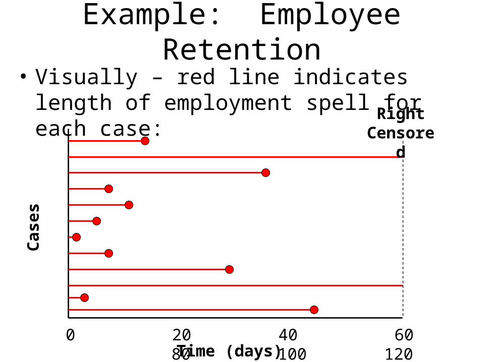
Example: Employee Retention
• Visually – red line indicates length of employment spell for each case:
0 20 40 60 80 100 120 Time (days)
Cas
es
Right Censored

Descriptives: Half Life
• Time when ½ of sample has had event:
0 20 40 60 80 100 120 Time (days)
Cas
es
Right Censored
Half Life = 23 days
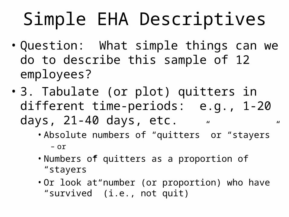
Simple EHA Descriptives
• Question: What simple things can we do to describe this sample of 12 employees?
• 3. Tabulate (or plot) quitters in different time-periods: e.g., 1-20 days, 21-40 days, etc.
• Absolute numbers of “quitters” or “stayers”– or
• Numbers of quitters as a proportion of “stayers”• Or look at number (or proportion) who have “survived”
(i.e., not quit)

Descriptives: Tables• For each period, determine number or
proportion quitting/staying
0 20 40 60 80 100 120 Time (days)
Cas
es
Day 1-20 20-40 40-60 60-80 80-100

EHA Descriptives: TablesTime Range
Quitters:
Total #, %
# staying
1 Day 1-20 5 quit, 42% of all,
42% of remaining
7 left, 58 % of all
2 Day 21-40 2 quit, 16% of all
29% of remaining
5 left, 42% of all
3 Day 41-60 1 quit, 8% of all
20% of remaining
4 left, 33 % of all
4 Day 61-80 1 quit, 8% of all
25% of remaining
3 left, 25% of all

EHA Descriptives: Tables
• Remarks on EHA tables:
• 1. Results of tables change depending on time-ranges chosen (like a histogram)
• E.g., comparing 20-day ranges vs. 10-day ranges
• 2. % quitters vs. % quitters as a proportion of those still employed
• Absolute % can be misleading since the number of people left in the risk set tends to decrease
• A low # of quitters can actually correspond to a very high rate of quitting for those remaining in the firm
• Typically, these ratios are more socially meaningful than raw percentages.

EHA Descriptives: Plots
• We can also plot tabular information:
0
10
20
30
40
50
60
70
80
90
100
0 1 2 3 4 5
Time Period
Pe
rce
nt
% Quit (of Remaining)
% Remaining

The Survivor Function
• A more sophisticated version of % remaining• Calculated based on continuous time (calculus), rather
than based on some arbitrary interval (e.g., day 1-20)
• Survivor Function – S(t): The probability (at time = t) of not having the event prior to time t.
• Always equal to 1 at time = 0 (when no events can have happened yet
• Decreases as more cases experience the event• When graphed, it is typically a decreasing curve• Looks a lot like % remaining.

Survivor Function
• McDonald’s Example:Survivor Function: McDonalds Employees
0
0.1
0.2
0.3
0.4
0.5
0.6
0.7
0.8
0.9
1
0 20 40 60 80 100 120
Time
S(t
)
Steep decreases indicate lots of
quitting at around 20 days

The Hazard Function
• A more sophisticated version of # events divided by # remaining
• Hazard Function – h(t) = The probability of an event occurring at a given point in time, given that it hasn’t already occurred
• Formula:
t
tTtTttPth
t
)(lim)(
0
• Think of it as: the rate of events occurring for those at risk of experiencing the event
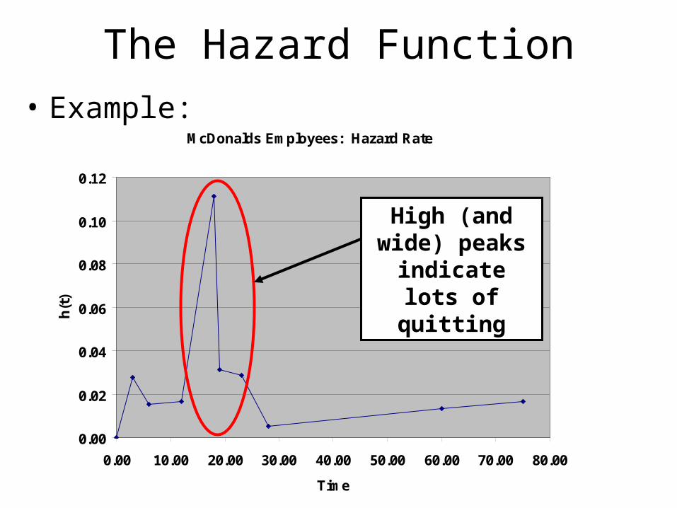
The Hazard Function
• Example:McDonalds Employees: Hazard Rate
0.00
0.02
0.04
0.06
0.08
0.10
0.12
0.00 10.00 20.00 30.00 40.00 50.00 60.00 70.00 80.00
Time
h(t
)
High (and wide) peaks indicate lots of quitting

Cumulative Hazard Function
• Problem: the Hazard Function is often very spiky and hard to read/interpret
• Alternative #1: “Smooth” the hazard function (using a smoothing algorithm)
• Alternative #2: The “cumulative” or “integrated” hazard
• Use calculus to “integrate” the hazard function• Recall – An integral represents the area under the
curve of another function between 0 and t.• Integrated hazard functions always increase (opposite
of the survivor function).• Big growth indicates that the hazard is high.

Integrated Hazard Function
• Example:McDonalds Employees: Integrated Hazard
0
0.2
0.4
0.6
0.8
1
1.2
1.4
1.6
1.8
0 20 40 60 80 100
Time
Inte
gra
ted
Haz
ard
Steep increases indicate peaks in
hazard rate
“Flat” areas indicate low hazard rate

Descriptive EHA: Marriage
• Example: Event = Marriage• Time Clock: Person’s Age• Data Source: NORC General Social Survey• Sample: 29,000 individuals

Survivor: Marriage
• Compare survivor for women, men:Kaplan-Meier survival estimates, by dfem
analysis time0 50 100
0.00
0.25
0.50
0.75
1.00
dfem 0
dfem 1
Survivor plot for Men
(declines later)
Survivor plot for Women
(declines earlier)
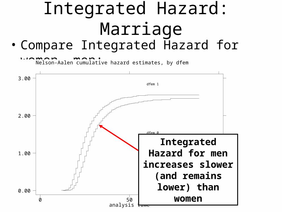
Integrated Hazard: Marriage
• Compare Integrated Hazard for women, men:Nelson-Aalen cumulative hazard estimates, by dfem
analysis time0 50 100
0.00
1.00
2.00
3.00
dfem 0
dfem 1
Integrated Hazard for men increases slower (and remains lower)
than women

Figure 3. Estimated hazard rateof entry into first marriage for entire sample
Est
ima
ted
Ha
zard
Ra
te
Age in Years12 20 30 40 50 60 70 80
12 20 30 40 50 60 70 80
0
.05
.1
.15
.2
0
.05
.1
.15
.2
Hazard Plot: Marriage• Hazard Rate: Full Sample

Survivor Plot: Pros/Cons
• Benefits: • 1. Clear, simple interpretation• 2. Useful for comparing subgroups in data
Limitations:• 1. Mainly useful for a fixed risk set with a single non-
repeating event (e.g., Drug trials/mortality)– If events recur frequently, the survivor drops to zero (and
becomes uninterpretable)
• 2. If the risk set fluctuates a lot, the survivor function becomes harder to interpret.

Hazard Plot Pros/Cons
• Benefits:• Directly shows the rate over time
– This is the actual dependent variable modeled
• Works well for repeating events
• Limitations:• Can be difficult to interpret – requires practice• Spikes make it hard to get a clear picture of trend
– Pay close attention to width of spikes, not just height!
• Choice of smoothing algorithms can affect results• Hard to compare groups (due to spikeyness).

Integrated Hazard Plot Pros/Cons
• Benefits:• Closely related to the dependent variable that you’ll be
modeling• Very good for comparing groups• Works for repeating events
• Limitations:• Not as intuitive as the actual hazard rate• Still takes some practice to interpret.

From Plots to Models
• We know from the plots that women get married faster than men
• Questions: – 1. how do we quantify the difference in hazard
rates?– 2. How do we test hypotheses about the
difference in rates?• Can we be confident that the observed difference
between men and women is not merely due to sampling variability

EHA Models
• Strategy:
• Model the hazard rate as a function of covariates
• Much like regression analysis
• Determine coefficients• The extent to which change in independent variables
results in a change in the hazard rate
• Use information from sample to compute t-values (and p-values)
• Test hypotheses about coefficients

EHA Models
• Issue: In standard regression, we must choose a proper “functional form” relating X’s to Y’s
• OLS is a “linear” model – assumes a liner relationship– e.g.: Y = a + b1X1 + b2X2 … + bnXn + e
• Logistic regression for discrete dependent variables – assumes an ‘S-curve’ relationship between variables
• When modeling the hazard rate h(t) over time, what relationship should we assume?
• There are many options: assume a flat hazard, or various S-shaped, U-shaped, or J-shaped curves
• We’ll discuss details later…
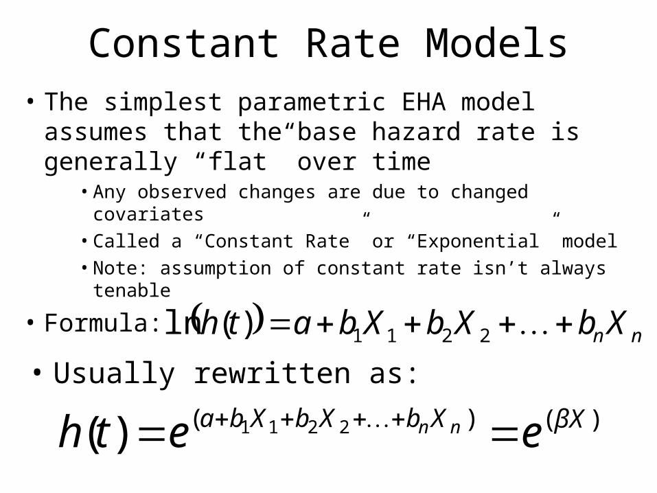
Constant Rate Models
• The simplest parametric EHA model assumes that the base hazard rate is generally “flat” over time
• Any observed changes are due to changed covariates• Called a “Constant Rate” or “Exponential” model• Note: assumption of constant rate isn’t always tenable
• Formula: nnXbXbXbath 2211)(ln
• Usually rewritten as:
)()( 2211)( βXXbXbXba eeth nn

Constant Rate Models• Question: Is the constant rate assumption
tenable?Figure 3. Estimated hazard rateof entry into first marriage for entire sample
Est
ima
ted
Ha
zard
Ra
te
Age in Years12 20 30 40 50 60 70 80
12 20 30 40 50 60 70 80
0
.05
.1
.15
.2
0
.05
.1
.15
.2

Constant Rate Models• Question: Is the constant rate assumption
tenable?
• Answer: Probably not• The hazard rate goes up and down over time
– Not constant at all – even if smoothed
• 2. The change over time isn’t likely the result of changing covariates (X’s) in our model
• However, if the change was merely the result of some independent variable, then the underlying (unobserved) rate might, in fact, be constant.

Constant Rate Models
• Let’s run an analysis anyway…
• Ignore the violation of assumptions regarding the functional form of the hazard rate Recall -- Constant rate model is:
)()( 2211)( βxXbXbXba nnn eeth
• In this case, we’ll only specify one X var:• DFEMALE – dummy variable indicating women• Coefficient reflects difference in hazard rate for women
versus men.

Constant Rate Model: Marriage
• A simple one-variable model comparing genderExponential regression
No. of subjects = 29269
No. of failures = 24108
Log likelihood = -30891.849 Prob > chi2 = 0.0000
--------------------------------------------------
_t | Coef. Std. Err. z P>|z|
--------+-----------------------------------------
Female | .1898716 .0130504 14.55 0.000
_cons | -3.465594 .0099415 -348.60 0.000
--------------------------------------------------
• The positive coefficient for Female (a dummy variable) indicates a higher hazard rate for women

Constant Rate Coefficients
• Interpreting the EHA coefficient: b = .19
• Coefficients reflect change in log of the hazard– Recall one of the ways to write the formula:
nnXbXbXbath 2211)(ln
• But – we aren’t interested in change in log rates
• We’re interested in change in the actual rate
• Solution: Exponentiate the coefficient• i.e., use “inverse-log” function on calculator• Result reflects the impact on the actual rate.

Constant Rate Coefficients
• Exponentiate the coefficient to generate the “hazard ratio”
Ratio Hazard21.1)19(.)( ee coef
• Multiplying by the hazard ratio indicates the increase in hazard rate for each unit increase in the independent variable
• Multiplying by 1.21 results in a 21% increase• A hazard ratio of 2.00 = a 200% increase• A hazard ratio of .25 = a decreased rate by 75%.

Constant Rate Coefficients
• The variable FEMALE is a dummy variable• Women = 1, Men = 0• Increase from 0 to 1 (men to women) reflects a 21%
increase in the hazard rate
– Continuous measures, however can change by many points (e.g., Firm size, age, etc.)
• To determine effects of multiple point increases (e.g., firm size of 10 vs. 7) multiply repeatedly
• Ex: Hazard Ratio = .95, increase = 3 units:• .95 x .95 x .95 = .86 – indicating a 14% decrease.

Hypothesis Tests: Marriage
• Final issue: Is the 21% higher hazard rate for women significantly different than men?
• Or is the observed difference likely due to chance?
• Solution: Hazard rate models calculate standard errors for coefficient estimates
• Allowing calculation of T-values, P-values
--------------------------------------------------
_t | Coef. Std. Err. t P>|t|
--------+---------------------------------------
Female | .1898716 .0130504 14.55 0.000
_cons | -3.465594 .0099415 -348.60 0.000
--------------------------------------------------

Types of EHA Models
• Two main types of proportional EHA Models
• 1. Parametric Models• specify a functional form of h(t)• Constant rate is one example• Also: Piecewise Exponential, Gompertz, Weibull,etc.
• 2. Cox Models• Doesn’t specify a particular form for h(t)
• Each makes assumptions• Like OLS assumptions regarding functional form, error
variance, normality, etc• If assumptions are violated, models can’t be trusted.

Parametric Models
• These models make assumptions about the overall shape of the hazard rate over time
• Much like OLS regression assumes a linear relationship between X and Y, logit assumes s-curve
• Options: constant, Gompertz, Weibull• There is a piecewise exponential option, too
• Note: They also make standard statistical assumptions:
• Independent random sample• Properly specified model, etc, etc…

Cox Models
• The basic Cox model:)(
02211)()( nnXbXbXbethth
• Where h(t) is the hazard rate
• h0(t) is some baseline hazard function (to be inferred from the data)• This obviates the need for building a specific
functional form into the model
• bX’s are coefficients and covariates

Cox Model Assumptions
• Cox Models assume that independent variables don’t interact with time
• At lease, not in ways you haven’t controlled for• i.e., that the hazard rate at different values of X are
proportional (parallel) to each other over time
• Example: Marriage rate – women vs. men• Women have a higher rate at all points in time
• Question: Does the hazard rate for women diverge or converge with men over time?
• If so, the proportion (or ratio) of the rate changes. The assumption is violated. Use a different model

Cox Model Assumptions:
• Proportionality: Look for parallel h(t)’s for different sub-groups (values of X’s)
h(t
)
time
Good
Women
Men
h(t
)
Bad
Women
Men

Cox Model Assumptions:
• Hazard rates are often too spiky to discern trends
• Options:
• 1. Smooth the hazard plots
OR
• 2. Check the integrated hazard rate– Look for differences in the overall shape of the
curve– Note: divergence is OK on an integrated hazard

Cox Model: Example
• Marriage example:
No. of subjects = 29269 Number of obs = 29269
No. of failures = 24108 Time at risk = 693938
LR chi2(1) = 1225.71
Log likelihood = -229548.82 Prob > chi2 =0.0000
--------------------------------------------------
_t | Coef. Std. Err. z P>|z|
--------+-----------------------------------------
Female | .4551652 .0131031 34.74 0.000
--------------------------------------------------
Related Documents