Evaluation of Wellhead Fatigue for Drilling Risers A Study on the Effect of Tension Kathrine Gregersen Marine Technology Supervisor: Svein Sævik, IMT Co-supervisor: Christian Revå, Aker Solutions Department of Marine Technology Submission date: June 2015 Norwegian University of Science and Technology

Welcome message from author
This document is posted to help you gain knowledge. Please leave a comment to let me know what you think about it! Share it to your friends and learn new things together.
Transcript
Evaluation of Wellhead Fatigue for Drilling RisersA Study on the Effect of Tension
Kathrine Gregersen
Marine Technology
Supervisor: Svein Sævik, IMTCo-supervisor: Christian Revå, Aker Solutions
Department of Marine Technology
Submission date: June 2015
Norwegian University of Science and Technology


NTNU Trondheim
Norges teknisk-naturvitenskapelige universitet
Institutt for marin teknikk
MASTER THESIS SPRING 2015
for
Stud. tech. Kathrine Gregersen
Evaluation of wellhead fatigue for drilling risers Vurdering av Brønnhodeutmatting av borestigerør
Wellhead fatigue as a result of work-over, drilling and completion is of interest. It is not
commonly understood how riser tension and water depth influence results. A better
understanding will ensure that a sufficiently conservative approach can be applied. According
to some references a large tension will give the highest fatigue damage. However, in some
projects a large tension yielded lower fatigue damage. Yet in other projects, a high tension
gave the highest damage. It is expected that the water depth and eigenfrequencies will
influence the results. Tension in this context is a result of both tension applied to the riser and
tension in the drill-string. Since the tension in the drill-string can vary significantly it is of
interest to know the level of total tension that yields the most fatigue damage. The over pull
may then be varied to reduce fatigue damage. The focus for the present master thesis is the
influence of applied tension on the fatigue damage. The basis for the study has already been
established during the project work including:
1. Literature study, including relevant standards for riser analysis and theoretical basis for
riser computational tools like Sima/Riflex, Flexcom etc. Also familiarization with the
tool be used during the numerical studies.
2. Basis for case studies in terms of load cases, vessel motions, hydrodynamic coefficients,
cross-section details, water depths and tension envelopes.
3. Global analysis model that can be used for further studies.
From the above basis, the work is to be continued focusing on investigating the parameters
governing the fatigue stresses of the wellhead by:
4. Establish basis for parameter study in terms of studying the effect of water depth (80m,
125m, 190m, 500m and 1000m), wellhead stiffness (mean +/-50%), over pull (25t-100
tons in steps of 10t) and environment scatter diagram (Base case Hs =3.5 m + all
periods).
5. Perform eigenvalue analysis of the above cases.

NTNU Fakultet for ingeniørvitenskap og teknologi
Norges teknisk-naturvitenskapelige universitet Institutt for marin teknikk
6. Perform regular/irregular analysis and investigate the fatigue responses in terms of
moment histograms and relative fatigue calculations using m=5 as exponent.
7. Identify the physical effects that govern the response in the different load cases
focusing on the role of overpull versus moment histogram behavior.
8. Conclusions and recommendations for further work
All necessary input data is assumed to be provided by Aker Solutions.
The work scope may prove to be larger than initially anticipated. Subject to approval from the
supervisors, topics may be deleted from the list above or reduced in extent.
In the thesis the candidate shall present his personal contribution to the resolution of problems
within the scope of the thesis work
Theories and conclusions should be based on mathematical derivations and/or logic reasoning
identifying the various steps in the deduction.
The candidate should utilise the existing possibilities for obtaining relevant literature.
Thesis format
The thesis should be organised in a rational manner to give a clear exposition of results,
assessments, and conclusions. The text should be brief and to the point, with a clear language.
Telegraphic language should be avoided.
The thesis shall contain the following elements: A text defining the scope, preface, list of
contents, summary, main body of thesis, conclusions with recommendations for further work, list
of symbols and acronyms, references and (optional) appendices. All figures, tables and
equations shall be numerated.
The supervisors may require that the candidate, in an early stage of the work, presents a written
plan for the completion of the work.
The original contribution of the candidate and material taken from other sources shall be clearly
defined. Work from other sources shall be properly referenced using an acknowledged
referencing system.
The report shall be submitted in two copies:
- Signed by the candidate
- The text defining the scope included
- In bound volume(s)
- Drawings and/or computer prints which cannot be bound should be organised in a separate
folder.
Ownership
NTNU has according to the present rules the ownership of the thesis. Any use of the thesis has to be
approved by NTNU (or external partner when this applies). The department has the right to use the
NTNU Fakultet for ingeniørvitenskap og teknologi
Norges teknisk-naturvitenskapelige universitet Institutt for marin teknikk
thesis as if the work was carried out by a NTNU employee, if nothing else has been agreed in
advance.
Thesis supervisors:
Prof. Svein Sævik, NTNU
Christian Revå, Aker Solutions
Deadline: June 10th, 2015
Trondheim, January 14th, 2015
Svein Sævik
Candidate – date and signature:


v
Preface
This master’s thesis is a mandatory part of the 5-year Master of Science program in Marine
Technology. The work has been carried out at the department of Marine Technology at the
Norwegian University of Science and Technology (NTNU). Aker Solutions has been collabora-
tor during this thesis. This thesis succeeds the project carried out in the fall of 2014, where a
literature study of wellhead fatigue was carried out. In addition, a global analysis model was
established.
During the beginning of the thesis work, a lot of time was used to establish the correct global
load analysis model, with all the necessary information. Research on wellhead fatigue has also
been an important part of this thesis. In addition, interpreting the results from global analysis
and fatigue calculations has been a major part of the work.
I would like to thank Aker Solutions and my supervisor, Christian Revå for coming up with an
idea for the thesis and for providing me with the necessary data. In addition, I want to thank
Elizabeth Passano and Anders Amundsen from MARINTEK, for helping me with software re-
lated issues. Last, but not least, I want to thank professor Svein Sævik for all the help he has
offered. The weekly guidance and discussions he has provided me with have been very impor-
tant in helping me complete my thesis.
Trondheim, 8th of June, 2015
————————————————————-
Kathrine Gregersen


vii
Summary
In the oil and gas industry today, there is a renewed focus on the structural integrity of the well-
head. There exist no codes or standards on how to calculate wellhead fatigue today. However,
a Joint Industry Project (JIP) was initiated to establish a Wellhead Fatigue Analysis Method
(DNV; 2011). Several uncertainties related to the modelling and simulation of global load anal-
yses were addressed in this report. In this thesis, the uncertainty related to how tension/over-
pull affects fatigue damage is investigated. Overpull is defined as the tension below the Lower
Marine Riser Package (LMRP). In the Joint Industry Project it was assumed that the highest
overpull would result in the highest fatigue damage (DNV; 2011).
A presentation of ongoing and previous work on wellhead fatigue is given. In addition, a de-
scription of the drilling riser system and relevant theory is presented. This includes theory
related to the dynamic analysis of risers, fatigue damage, and a short overview of the wellhead
fatigue analysis method.
A case study is conducted by applying different water depths (80-1000 m), wellhead stiffnesses,
and overpulls in the range of 25-100 t. The global load analyses are carried out in SIMA/RI-
FLEX, which is a finite element software for slender marine structures. Irregular waves are ap-
plied using a JONSWAP spectrum with Hs=3.5 m and Tp=4.5-20.5 sec. In addition, a uniform
current, u=0.05 m/s, is applied. Both waves and current are applied in the same direction. The
simulation length used is 1 hour. The relative fatigue damage is assessed applying SN-curves
and Miner-Palmgren summation. In addition, bending moment histograms are produced for
each case. The term relative damage is used since the fatigue calculation applies moments
instead of stress in the calculations. It is assumed that the stress is linearly dependent on the
bending moment, thus the fatigue damage calculated will be proportional to the actual fatigue
damage.
The results from the global load analysis show that the lowest overpull (25 t) have the highest
number of cycles for the high bending moment range. Hence, high fatigue damage is expected
for this overpull. A low overpull leads to a very flexible system, resulting in large motion of
the wellhead (load controlled behaviour). The largest overpulls (90 - 100 t) are seen to have
a peak in its number of cycles for the second largest bending moment range. For high over-
pulls, the system is stiff, resulting in high axial forces on the wellhead (displacement controlled
behaviour). Investigating a middle overpull of 80 t shows that it has a peak number of cycles
for a lower bending moment range, thus resulting in a damage minima. When comparing the
different water depths, it is observed that the bending moment reduces for increasing depths,
thus the fatigue damage is reduced for increasing water depth. It is also found that reducing
the wellhead stiffness increase the bending moment range where the peak in the number of
cycles occurs, thus resulting in higher damage. The fatigue damage calculated can be seen for
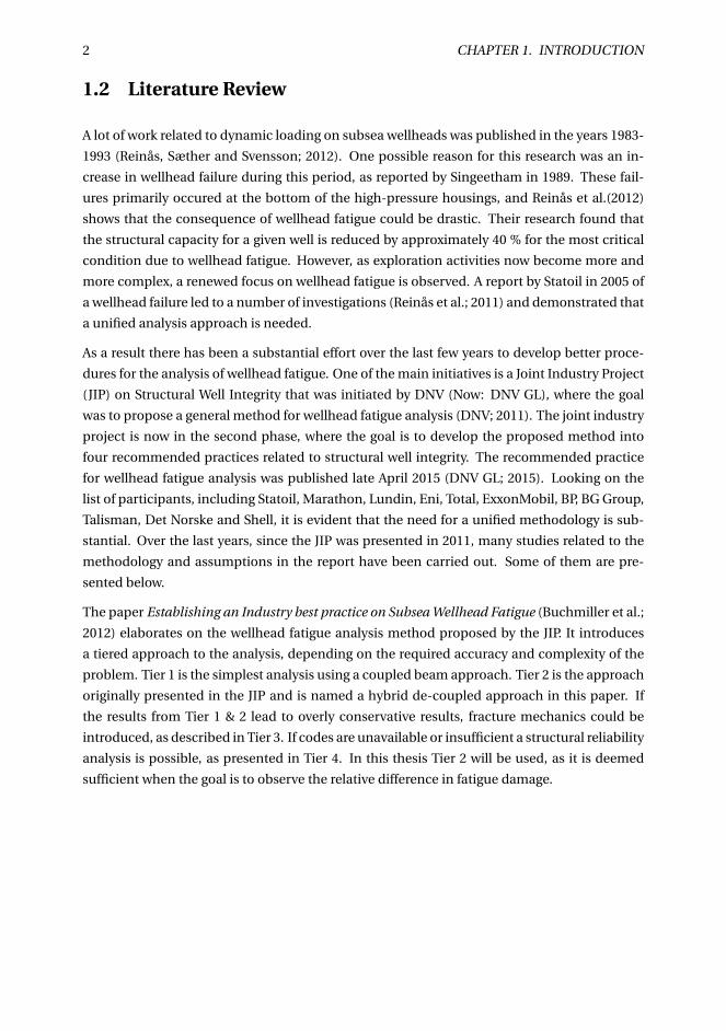
a variation in overpull and water depth in Figure 1.
viii
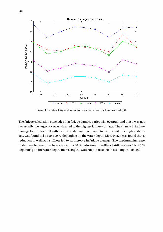
Figure 1: Relative fatigue damage for variation in overpull and water depth
The fatigue calculation concludes that fatigue damage varies with overpull, and that it was not
necessarily the largest overpull that led to the highest fatigue damage. The change in fatigue
damage for the overpull with the lowest damage, compared to the one with the highest dam-
age, was found to be 190-600 %, depending on the water depth. Moreover, it was found that a
reduction in wellhead stiffness led to an increase in fatigue damage. The maximum increase
in damage between the base case and a 50 % reduction in wellhead stiffness was 75-140 %
depending on the water depth. Increasing the water depth resulted in less fatigue damage.

ix
Sammendrag
I olje- og gassindustrien i dag er det et fornyet fokus på brønnhodets strukturelle integritet.
Per dags dato finnes det ingen koder eller standarder for hvordan man beregner brønnhodeut-
matting. Et felles industriprosjekt ble imidlertid igangsatt for å etablere en felles analyseme-
tode for brønnhodeutmatting (DNV; 2011). Flere usikkerheter knyttet til modellering og simu-
lering av globale last analyser ble tatt opp i denne rapporten. I denne masteroppgaven er
usikkerheten knyttet til hvordan strekk/overtrekk (tension/overpull) påvirker utmatting blitt
undersøkt. Overtrekk er definert som strekket under Lower Marine Riser Package (LMRP). I
industriprosjektet ble det antatt at det høyeste overtrekket vil resultere i den høyeste utmat-
tingsskaden (DNV; 2011).
En presentasjon av tidligere- og pågående arbeid relatert til brønnhodeutmatting er gitt. I til-
legg er en beskrivelse av borestigerørssystemet og relevant teori er presentert. Dette omfatter
teori relatert til den dynamiske analysen av stigerør, utmattingsberegninger og en kort gjen-
nomgang av analysemetoden for beregning av brønnhodeutmatting.
En casestudie er gjennomført ved å undersøke ulike havdyp (80-1000 m), brønnhodestivheter
og overtrekk i området fra 25 til 100 t. De globale last analysene er utført i SIMA / RIFLEX,
som er en programvare for FEM-analyse av slanke marine konstruksjoner. Irregulære bølger
påføres ved bruk av et JONSWAP spektrum med Hs = 3.5 m og Tp = 4.5-20.5 sek. I tillegg
er en uniform strøm, u = 0.05 m / s, påført. Både bølger og strøm blir påført i den samme
retningen. En time simuleringslengden er brukt. Den relative utmattingsskaden estimeres
ved bruk av SN-kurver og Miner-Palmgren sum. I tillegg er momenthistogrammer produsert.
Uttrykket relativ skade (relative damage) er anvendt ettersom utmattingsskaden er basert på
moment i stedet for spenning i beregningen. Det antas at spenningen er lineært avhengig av
bøyemomentet, og dermed vil den beregnede utmattingsskaden være proporsjonal med den
faktiske utmattingsskaden.
Resultatene fra den globale last analysen viser at det laveste overtrekket (25 t) har det høyeste
antall sykluser for høy bøyemoment range (variasjonsbredde). Derfor er høye utmattingsskader
forventet for dette overtrekket. Et lavt overtrekk fører til et meget fleksibelt system, som resul-
terer i stor bevegelse av brønnhodet (laststyrt oppførsel). De største overtrekkene (90-100 t) er
sett til å ha en topp i antall sykluser for den nest største bøyemoment rangen. Høyt overtrekk
gir et stivt system, noe som resulterer i høye aksielle krefter på brønnhodet (forskyvningsstyrt
oppførsel). Undersøkelser av 80 t overtrekk viser at den har en topp i antall sykluser for en la-
vere bøyemoment område, noe som resulterer i lavest skade. Ved sammenligning av de ulike
vanndybdene er det observert at bøyemomentet reduseres for økende vanndyp, og dermed
reduseres utmattingsskaden for økende vanndyp. I tillegg er det er observert at en reduksjon i
brønnhodestivheten øker bøyemomentet rangen hvor toppen i antall sykluser finner sted, noe
som resulterer i høyere skade. Den beregnede utmattingsskaden kan sees for en variasjon av
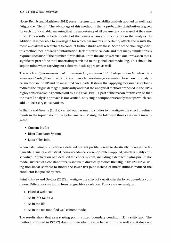
overtrekk og vanndybder i Figur 2.
x
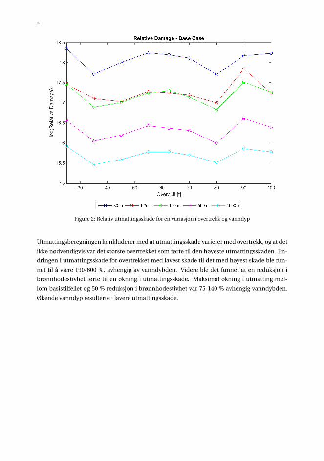
Figure 2: Relativ utmattingsskade for en variasjon i overtrekk og vanndyp
Utmattingsberegningen konkluderer med at utmattingsskade varierer med overtrekk, og at det
ikke nødvendigvis var det største overtrekket som førte til den høyeste utmattingsskaden. En-
dringen i utmattingsskade for overtrekket med lavest skade til det med høyest skade ble fun-
net til å være 190-600 %, avhengig av vanndybden. Videre ble det funnet at en reduksjon i
brønnhodestivhet førte til en økning i utmattingsskade. Maksimal økning i utmatting mel-
lom basistilfellet og 50 % reduksjon i brønnhodestivhet var 75-140 % avhengig vanndybden.
Økende vanndyp resulterte i lavere utmattingsskade.
Contents
Problem text . . . . . . . . . . . . . . . . . . . . . . . . . . . . . . . . . . . . . . . . . . . . i
Preface . . . . . . . . . . . . . . . . . . . . . . . . . . . . . . . . . . . . . . . . . . . . . . . v
Summary . . . . . . . . . . . . . . . . . . . . . . . . . . . . . . . . . . . . . . . . . . . . . . vii
Sammendrag . . . . . . . . . . . . . . . . . . . . . . . . . . . . . . . . . . . . . . . . . . . ix
Nomenclature . . . . . . . . . . . . . . . . . . . . . . . . . . . . . . . . . . . . . . . . . . . xxiii
1 Introduction 1
1.1 Background . . . . . . . . . . . . . . . . . . . . . . . . . . . . . . . . . . . . . . . . . 1
1.2 Literature Review . . . . . . . . . . . . . . . . . . . . . . . . . . . . . . . . . . . . . . 2
1.3 Objective . . . . . . . . . . . . . . . . . . . . . . . . . . . . . . . . . . . . . . . . . . . 4
1.4 Scope and Limitations . . . . . . . . . . . . . . . . . . . . . . . . . . . . . . . . . . . 5
1.5 Thesis Structure . . . . . . . . . . . . . . . . . . . . . . . . . . . . . . . . . . . . . . . 5
2 System Description 7
2.1 Drilling Facilities . . . . . . . . . . . . . . . . . . . . . . . . . . . . . . . . . . . . . . 8
2.2 Drilling Process . . . . . . . . . . . . . . . . . . . . . . . . . . . . . . . . . . . . . . . 9
2.3 Riser Types . . . . . . . . . . . . . . . . . . . . . . . . . . . . . . . . . . . . . . . . . . 11
2.4 Marine Riser System . . . . . . . . . . . . . . . . . . . . . . . . . . . . . . . . . . . . 12
2.4.1 Top Assembly . . . . . . . . . . . . . . . . . . . . . . . . . . . . . . . . . . . . 13
2.4.2 Riser . . . . . . . . . . . . . . . . . . . . . . . . . . . . . . . . . . . . . . . . . 14
2.4.3 Lower Stack . . . . . . . . . . . . . . . . . . . . . . . . . . . . . . . . . . . . . 15
3 Dynamic Theory 17
3.1 Finite Element Model . . . . . . . . . . . . . . . . . . . . . . . . . . . . . . . . . . . 17
3.1.1 Mass Matrix . . . . . . . . . . . . . . . . . . . . . . . . . . . . . . . . . . . . . 18
3.1.2 Stiffness Matrix . . . . . . . . . . . . . . . . . . . . . . . . . . . . . . . . . . . 19
3.1.3 Damping Matrix . . . . . . . . . . . . . . . . . . . . . . . . . . . . . . . . . . 20
3.2 Static Analysis . . . . . . . . . . . . . . . . . . . . . . . . . . . . . . . . . . . . . . . . 21
3.3 Eigenvalue Analysis . . . . . . . . . . . . . . . . . . . . . . . . . . . . . . . . . . . . . 22
3.4 Dynamic Time Domain Analysis . . . . . . . . . . . . . . . . . . . . . . . . . . . . . 24
3.5 Effective Tension . . . . . . . . . . . . . . . . . . . . . . . . . . . . . . . . . . . . . . 25
3.6 Hydrodynamic Loads . . . . . . . . . . . . . . . . . . . . . . . . . . . . . . . . . . . . 26
xi
xii CONTENTS
3.7 Stochastic Theory . . . . . . . . . . . . . . . . . . . . . . . . . . . . . . . . . . . . . . 28
4 Fatigue Theory 31
4.1 Fatigue Damage . . . . . . . . . . . . . . . . . . . . . . . . . . . . . . . . . . . . . . . 31
4.2 Load History . . . . . . . . . . . . . . . . . . . . . . . . . . . . . . . . . . . . . . . . . 32
4.3 S-N Curves . . . . . . . . . . . . . . . . . . . . . . . . . . . . . . . . . . . . . . . . . . 34
4.4 Cycle Counting . . . . . . . . . . . . . . . . . . . . . . . . . . . . . . . . . . . . . . . 36
4.5 Histogram . . . . . . . . . . . . . . . . . . . . . . . . . . . . . . . . . . . . . . . . . . 38
4.6 Miner-Palmgren Summation . . . . . . . . . . . . . . . . . . . . . . . . . . . . . . . 39
5 Overall Wellhead Fatigue Methodology 41
5.1 Local Response Analysis . . . . . . . . . . . . . . . . . . . . . . . . . . . . . . . . . . 42
5.1.1 Modelling . . . . . . . . . . . . . . . . . . . . . . . . . . . . . . . . . . . . . . 42
5.1.2 Wellhead Stiffness . . . . . . . . . . . . . . . . . . . . . . . . . . . . . . . . . 43
5.1.3 Load-to-stress Curve . . . . . . . . . . . . . . . . . . . . . . . . . . . . . . . . 44
5.2 Global Load Analysis . . . . . . . . . . . . . . . . . . . . . . . . . . . . . . . . . . . . 45
5.2.1 Modelling . . . . . . . . . . . . . . . . . . . . . . . . . . . . . . . . . . . . . . 45
5.3 Fatigue Damage Assessment . . . . . . . . . . . . . . . . . . . . . . . . . . . . . . . 47
6 Modelling and Analysis 49
6.1 Global Load Analysis . . . . . . . . . . . . . . . . . . . . . . . . . . . . . . . . . . . . 49
6.1.1 SIMA/RIFLEX . . . . . . . . . . . . . . . . . . . . . . . . . . . . . . . . . . . . 49
6.1.2 Input Data . . . . . . . . . . . . . . . . . . . . . . . . . . . . . . . . . . . . . . 51
6.1.3 Tension . . . . . . . . . . . . . . . . . . . . . . . . . . . . . . . . . . . . . . . . 54
6.1.4 Buoyancy . . . . . . . . . . . . . . . . . . . . . . . . . . . . . . . . . . . . . . . 55
6.1.5 Environment . . . . . . . . . . . . . . . . . . . . . . . . . . . . . . . . . . . . 56
6.1.6 Vessel Motion . . . . . . . . . . . . . . . . . . . . . . . . . . . . . . . . . . . . 57
6.1.7 Simulation . . . . . . . . . . . . . . . . . . . . . . . . . . . . . . . . . . . . . . 57
6.2 Fatigue Damage Assessment . . . . . . . . . . . . . . . . . . . . . . . . . . . . . . . 58
7 Presentation and Evaluation of Results 61
7.1 Global Load Analysis . . . . . . . . . . . . . . . . . . . . . . . . . . . . . . . . . . . . 61
7.1.1 Eigenvalue Analysis . . . . . . . . . . . . . . . . . . . . . . . . . . . . . . . . . 61
7.1.2 Bending Moment . . . . . . . . . . . . . . . . . . . . . . . . . . . . . . . . . . 71
7.1.3 Response Analysis . . . . . . . . . . . . . . . . . . . . . . . . . . . . . . . . . 74
7.2 Fatigue . . . . . . . . . . . . . . . . . . . . . . . . . . . . . . . . . . . . . . . . . . . . 82
7.2.1 Histograms . . . . . . . . . . . . . . . . . . . . . . . . . . . . . . . . . . . . . 82
7.2.2 Damage Calculations . . . . . . . . . . . . . . . . . . . . . . . . . . . . . . . . 92
7.3 Analytical Model . . . . . . . . . . . . . . . . . . . . . . . . . . . . . . . . . . . . . . 97
7.3.1 Displacement Model . . . . . . . . . . . . . . . . . . . . . . . . . . . . . . . . 98
7.3.2 Load Model . . . . . . . . . . . . . . . . . . . . . . . . . . . . . . . . . . . . . 98
7.3.3 Trend Line . . . . . . . . . . . . . . . . . . . . . . . . . . . . . . . . . . . . . . 99
7.4 Sensitivity Studies . . . . . . . . . . . . . . . . . . . . . . . . . . . . . . . . . . . . . . 100
CONTENTS xiii
7.4.1 Numerical Accuracy . . . . . . . . . . . . . . . . . . . . . . . . . . . . . . . . 101
7.4.2 Seed Number . . . . . . . . . . . . . . . . . . . . . . . . . . . . . . . . . . . . 102
7.4.3 Simulation Length . . . . . . . . . . . . . . . . . . . . . . . . . . . . . . . . . 103
7.4.4 Regular vs. Irregular Waves . . . . . . . . . . . . . . . . . . . . . . . . . . . . 104
7.4.5 Current . . . . . . . . . . . . . . . . . . . . . . . . . . . . . . . . . . . . . . . . 105
7.4.6 Possible Wellhead Resonance . . . . . . . . . . . . . . . . . . . . . . . . . . . 105
7.4.7 The Effect of Vessel Motion . . . . . . . . . . . . . . . . . . . . . . . . . . . . 107
7.4.8 Concluding Remarks . . . . . . . . . . . . . . . . . . . . . . . . . . . . . . . . 109
7.5 Uncertainties . . . . . . . . . . . . . . . . . . . . . . . . . . . . . . . . . . . . . . . . 110
7.5.1 Modelling . . . . . . . . . . . . . . . . . . . . . . . . . . . . . . . . . . . . . . 110
7.5.2 Drag Coefficient . . . . . . . . . . . . . . . . . . . . . . . . . . . . . . . . . . . 110
7.5.3 First Order Motion Function . . . . . . . . . . . . . . . . . . . . . . . . . . . 111
7.5.4 Seed Number . . . . . . . . . . . . . . . . . . . . . . . . . . . . . . . . . . . . 111
7.5.5 Vortex Induced Vibrations . . . . . . . . . . . . . . . . . . . . . . . . . . . . . 112
7.5.6 Environmental Condition . . . . . . . . . . . . . . . . . . . . . . . . . . . . . 112
7.5.7 S-N Curve . . . . . . . . . . . . . . . . . . . . . . . . . . . . . . . . . . . . . . 113
7.5.8 Miner-Palmgren Summation . . . . . . . . . . . . . . . . . . . . . . . . . . . 113
7.5.9 Block Division . . . . . . . . . . . . . . . . . . . . . . . . . . . . . . . . . . . . 113
7.6 Limitations . . . . . . . . . . . . . . . . . . . . . . . . . . . . . . . . . . . . . . . . . . 114
8 Conclusion 115
9 Further Work 117
Bibliography 119
A Riser Input Data I
A.1 Stack Up . . . . . . . . . . . . . . . . . . . . . . . . . . . . . . . . . . . . . . . . . . . I
A.2 Riser Properties . . . . . . . . . . . . . . . . . . . . . . . . . . . . . . . . . . . . . . . II
A.3 Hydrodynamic Coefficients . . . . . . . . . . . . . . . . . . . . . . . . . . . . . . . . II
A.4 Wellhead Stiffness . . . . . . . . . . . . . . . . . . . . . . . . . . . . . . . . . . . . . . III
A.5 Flex Joint Data . . . . . . . . . . . . . . . . . . . . . . . . . . . . . . . . . . . . . . . . III
B Top Tension Calculation V
B.1 80 m Water Depth . . . . . . . . . . . . . . . . . . . . . . . . . . . . . . . . . . . . . . V
B.2 125 m Water Depth . . . . . . . . . . . . . . . . . . . . . . . . . . . . . . . . . . . . . VI
B.3 190 m Water Depth . . . . . . . . . . . . . . . . . . . . . . . . . . . . . . . . . . . . . VII
B.4 500 m Water Depth . . . . . . . . . . . . . . . . . . . . . . . . . . . . . . . . . . . . . VIII
B.5 1000 m Water Depth . . . . . . . . . . . . . . . . . . . . . . . . . . . . . . . . . . . . IX
C Buoyancy Element Calculations XI
D Response Amplitude Operators XIII
xiv CONTENTS
E Eigenvalues XVII
E.1 80 m Water Depth . . . . . . . . . . . . . . . . . . . . . . . . . . . . . . . . . . . . . . XVII
E.2 125 m Water Depth . . . . . . . . . . . . . . . . . . . . . . . . . . . . . . . . . . . . . XIX
E.3 190 m Water Depth . . . . . . . . . . . . . . . . . . . . . . . . . . . . . . . . . . . . . XX
E.4 500 m Water Depth . . . . . . . . . . . . . . . . . . . . . . . . . . . . . . . . . . . . . XXI
E.5 1000 m Water Depth . . . . . . . . . . . . . . . . . . . . . . . . . . . . . . . . . . . . XXII
F Response Spectra XXIII
F.1 125 m Water Depth . . . . . . . . . . . . . . . . . . . . . . . . . . . . . . . . . . . . . XXIII
F.1.1 Variation in Overpull . . . . . . . . . . . . . . . . . . . . . . . . . . . . . . . . XXIII
F.1.2 Variation in Peak Period . . . . . . . . . . . . . . . . . . . . . . . . . . . . . . XXVIII
F.2 1000 m Water Depth . . . . . . . . . . . . . . . . . . . . . . . . . . . . . . . . . . . . XXXVII
F.2.1 Variation in Overpull . . . . . . . . . . . . . . . . . . . . . . . . . . . . . . . . XXXVII
F.2.2 Variation in Peak Period . . . . . . . . . . . . . . . . . . . . . . . . . . . . . . XLII
G Histograms LI
G.1 Overpull Comparison . . . . . . . . . . . . . . . . . . . . . . . . . . . . . . . . . . . LI
G.2 Water Depth Comparison . . . . . . . . . . . . . . . . . . . . . . . . . . . . . . . . . LIV
G.3 Wellhead Stiffness Comparison . . . . . . . . . . . . . . . . . . . . . . . . . . . . . . LIX
G.3.1 80 m Water Depth . . . . . . . . . . . . . . . . . . . . . . . . . . . . . . . . . . LIX
G.3.2 125 m Water Depth . . . . . . . . . . . . . . . . . . . . . . . . . . . . . . . . . LXIV
G.3.3 190 m Water Depth . . . . . . . . . . . . . . . . . . . . . . . . . . . . . . . . . LXIX
G.3.4 500 m Water Depth . . . . . . . . . . . . . . . . . . . . . . . . . . . . . . . . . LXXIV
G.3.5 1000 m Water Depth . . . . . . . . . . . . . . . . . . . . . . . . . . . . . . . . LXXIX
H Damage LXXXV
I Trend Line LXXXVII
J Wellhead Eigenvalues LXXXIX
K Contents in Attached Zip-file XCI

List of Figures
1 Relative fatigue damage for variation in overpull and water depth . . . . . . . . . viii
2 Relativ utmattingsskade for en variasjon i overtrekk og vanndyp . . . . . . . . . . x
2.1 Overview of phases in oil & gas recovery . . . . . . . . . . . . . . . . . . . . . . . . 7
2.2 Drilling rigs . . . . . . . . . . . . . . . . . . . . . . . . . . . . . . . . . . . . . . . . . 8
2.3 Drilling fluid circulation system . . . . . . . . . . . . . . . . . . . . . . . . . . . . . 9
2.4 Schematic illustration of the different steps for drilling a well from a floater . . . 10
2.5 Illustration of top tensioned riser . . . . . . . . . . . . . . . . . . . . . . . . . . . . . 11
2.6 Marine riser system and associated equipment . . . . . . . . . . . . . . . . . . . . 12
2.7 Illustration of tensioning system . . . . . . . . . . . . . . . . . . . . . . . . . . . . . 14
2.8 Schematic illustration of the wellhead system . . . . . . . . . . . . . . . . . . . . . 16
3.1 Linear 2D beam element . . . . . . . . . . . . . . . . . . . . . . . . . . . . . . . . . . 18
3.2 3D beam element . . . . . . . . . . . . . . . . . . . . . . . . . . . . . . . . . . . . . . 20
3.3 Static solution procedure . . . . . . . . . . . . . . . . . . . . . . . . . . . . . . . . . 22
3.4 Deformation described as a sum of eigenvectors . . . . . . . . . . . . . . . . . . . 23
3.5 Constant initial acceleration . . . . . . . . . . . . . . . . . . . . . . . . . . . . . . . 24
3.6 Constant average acceleration . . . . . . . . . . . . . . . . . . . . . . . . . . . . . . 24
3.7 Linear acceleration . . . . . . . . . . . . . . . . . . . . . . . . . . . . . . . . . . . . . 24
3.8 Variation of inertia and drag for a regular wave . . . . . . . . . . . . . . . . . . . . . 27
4.1 Crack growth curve . . . . . . . . . . . . . . . . . . . . . . . . . . . . . . . . . . . . . 32
4.2 Example of a load history . . . . . . . . . . . . . . . . . . . . . . . . . . . . . . . . . 33
4.3 S-N curve: Constant amplitude loading . . . . . . . . . . . . . . . . . . . . . . . . . 35
4.4 Bilinear S-N curve: Variable amplitude loading . . . . . . . . . . . . . . . . . . . . 35
4.5 Strain history and stress-strain response . . . . . . . . . . . . . . . . . . . . . . . . 37
4.6 Pagoda roof rainflow analogy . . . . . . . . . . . . . . . . . . . . . . . . . . . . . . . 37
4.7 Illustration of calculation of short-term histogram . . . . . . . . . . . . . . . . . . 38
4.8 Illustration of calculation of long-term histogram . . . . . . . . . . . . . . . . . . . 39
5.1 Analysis flowchart for wellhead fatigue methodology . . . . . . . . . . . . . . . . . 42
5.2 Lower boundary condition model . . . . . . . . . . . . . . . . . . . . . . . . . . . . 43
xv
xvi LIST OF FIGURES
5.3 Mode shapes that dominate the response of the wellhead system . . . . . . . . . 43
5.4 Examples of load curves with typical points . . . . . . . . . . . . . . . . . . . . . . 44
5.5 Example of a load-to-stress curve . . . . . . . . . . . . . . . . . . . . . . . . . . . . 45
5.6 Main components in the riser model for the three phases: Drilling, completion,
and workover . . . . . . . . . . . . . . . . . . . . . . . . . . . . . . . . . . . . . . . . 46
5.7 Example of non-linear stiffness of a flex joint . . . . . . . . . . . . . . . . . . . . . . 47
6.1 RIFLEX program structure and its modules . . . . . . . . . . . . . . . . . . . . . . . 50
6.2 Overview of the main building stones in RIFLEX . . . . . . . . . . . . . . . . . . . . 50
6.3 Riser stack up in drilling mode . . . . . . . . . . . . . . . . . . . . . . . . . . . . . . 52
6.4 Lower boundary condition model . . . . . . . . . . . . . . . . . . . . . . . . . . . . 54
6.5 Definition of external wrapping in SIMA/RIFLEX . . . . . . . . . . . . . . . . . . . 55
6.6 First order motion transfer function for surge . . . . . . . . . . . . . . . . . . . . . 57
7.1 Natural period for different overpulls and eigenvalue number (80 m) . . . . . . . 62
7.2 Natural period for different water depths and eigenvalue number (25 t) . . . . . . 63
7.3 Natural period for different wellhead stiffness (25 t, 80 m) . . . . . . . . . . . . . . 64
7.4 Overpull variation: Mode shape: Eigenvector 1 - X-displacement . . . . . . . . . . 65
7.5 Overpull variation: Mode shape: Eigenvector 3 - X-displacement . . . . . . . . . . 66
7.6 Water depth variation: Mode shape: Eigenvector 1 - X-displacement . . . . . . . . 67
7.7 Water depth variation: Mode shape: Eigenvector 3 - X-displacement . . . . . . . . 67
7.8 WH stiffness variation: Mode shape: Eigenvector 1 - X-displacement . . . . . . . 68
7.9 WH stiffness variation: Mode shape: Eigenvector 3 - X-displacement . . . . . . . 69
7.10 Eigenvalue "0" . . . . . . . . . . . . . . . . . . . . . . . . . . . . . . . . . . . . . . . . 70
7.11 Bending moment envelope (125 m, 62.5 t, Tp =4.5) . . . . . . . . . . . . . . . . . . 72
7.12 Standard deviation of bending moment envelope (125 m, 62.5 t, Tp =4.5) . . . . . 73
7.13 Response spectrum . . . . . . . . . . . . . . . . . . . . . . . . . . . . . . . . . . . . . 74
7.14 Wellhead response: 25 t overpull (Tp =9.5 sec, 125 m) . . . . . . . . . . . . . . . . . 76
7.15 Wellhead response: 100 t overpull (Tp =9.5 sec, 125 m) . . . . . . . . . . . . . . . . 77
7.16 Wellhead response: Tp =4.5 sec (62.5 t, 125 m) . . . . . . . . . . . . . . . . . . . . . 78
7.17 JONSWAP spectrum for Tp =4.5 sec . . . . . . . . . . . . . . . . . . . . . . . . . . . 78
7.18 Wellhead response: Tp =8.5 sec (62.5 t, 125 m) . . . . . . . . . . . . . . . . . . . . . 79
7.19 Wellhead response: 25 t overpull (Tp =9.5 sec, 1000 m) . . . . . . . . . . . . . . . . 80
7.20 Wellhead response: Tp =4.5 sec (62.5 t, 1000 m) . . . . . . . . . . . . . . . . . . . . 81
7.21 Wellhead response: Tp =13.5 sec (62.5 t, 1000 m) . . . . . . . . . . . . . . . . . . . . 82
7.22 Bending moment histogram: Overpull variation - 80 m . . . . . . . . . . . . . . . . 84
7.23 Bending moment histogram: Overpull variation - 125 m . . . . . . . . . . . . . . . 85
7.24 Bending moment histogram: Overpull variation - 190 m . . . . . . . . . . . . . . . 86
7.25 Bending moment histogram: Overpull variation - 500 m . . . . . . . . . . . . . . . 87
7.26 Bending moment histogram: Overpull variation - 1000 m . . . . . . . . . . . . . . 88
7.27 Bending moment histogram: Water depth comparison - overpull 25 t . . . . . . . 90
7.28 Bending moment histogram: Wellhead stiffness comparison - 80 m - overpull 25 t 92
LIST OF FIGURES xvii
7.29 Relative damage: Base case . . . . . . . . . . . . . . . . . . . . . . . . . . . . . . . . 93
7.30 Relative damage: Comparison of change in WH stiffness . . . . . . . . . . . . . . . 96
7.31 Analytical models applied to obtain trend line . . . . . . . . . . . . . . . . . . . . . 97
7.32 Trend line . . . . . . . . . . . . . . . . . . . . . . . . . . . . . . . . . . . . . . . . . . 99
7.33 Relative damage: Change in numerical accuracy . . . . . . . . . . . . . . . . . . . 101
7.34 Relative damage: Change in seed number . . . . . . . . . . . . . . . . . . . . . . . 102
7.35 Relative damage: Change in simulation length . . . . . . . . . . . . . . . . . . . . . 103
7.36 Relative damage: Comparison of regular and irregular waves . . . . . . . . . . . . 104
7.37 Relative damage: The effect of current . . . . . . . . . . . . . . . . . . . . . . . . . . 105
7.38 Analytical model for calculation of wellhead eigenvalue . . . . . . . . . . . . . . . 106
7.39 Relative damage: Change in wellhead stiffness . . . . . . . . . . . . . . . . . . . . . 107
7.40 Relative damage: Effect of vessel motion - 125 m water depth . . . . . . . . . . . . 108
7.41 Relative damage: Effect of vessel motion - 1000 m water depth . . . . . . . . . . . 109
7.42 Relation between drag coefficient and Reynolds number for a circular cylinder . 111
A.1 Lower BC model . . . . . . . . . . . . . . . . . . . . . . . . . . . . . . . . . . . . . . . III
D.1 Surge RAO: Amplitude, head sea . . . . . . . . . . . . . . . . . . . . . . . . . . . . . XIII
D.2 Surge RAO: Phase, head sea . . . . . . . . . . . . . . . . . . . . . . . . . . . . . . . . XIII
D.3 Heave RAO: Amplitude, head sea . . . . . . . . . . . . . . . . . . . . . . . . . . . . . XIV
D.4 Heave RAO: Phase, head sea . . . . . . . . . . . . . . . . . . . . . . . . . . . . . . . . XIV
D.5 Pitch RAO: Amplitude, head sea . . . . . . . . . . . . . . . . . . . . . . . . . . . . . XV
D.6 Pitch RAO: Phase, head sea . . . . . . . . . . . . . . . . . . . . . . . . . . . . . . . . XV
F.1 Wellhead response: 25 t overpull (Tp =9.5 sec, 125 m) . . . . . . . . . . . . . . . . . XXIII
F.2 Wellhead response: 35 t overpull (Tp =9.5 sec, 125 m) . . . . . . . . . . . . . . . . . XXIV
F.3 Wellhead response: 45 t overpull (Tp =9.5 sec, 125 m) . . . . . . . . . . . . . . . . . XXIV
F.4 Wellhead response: 55 t overpull (Tp =9.5 sec, 125 m) . . . . . . . . . . . . . . . . . XXV
F.5 Wellhead response: 62.5 t overpull (Tp =9.5 sec, 125 m) . . . . . . . . . . . . . . . . XXV
F.6 Wellhead response: 70 t overpull (Tp =9.5 sec, 125 m) . . . . . . . . . . . . . . . . . XXVI
F.7 Wellhead response: 80 t overpull (Tp =9.5 sec, 125 m) . . . . . . . . . . . . . . . . . XXVI
F.8 Wellhead response: 90 t overpull (Tp =9.5 sec, 125 m) . . . . . . . . . . . . . . . . . XXVII
F.9 Wellhead response: 100 t overpull (Tp =9.5 sec, 125 m) . . . . . . . . . . . . . . . . XXVII
F.10 Wellhead response: Tp =4.5 sec (62.5 t, 125 m) . . . . . . . . . . . . . . . . . . . . . XXVIII
F.11 Wellhead response: Tp =5.5 sec (62.5 t, 125 m) . . . . . . . . . . . . . . . . . . . . . XXIX
F.12 Wellhead response: Tp =6.5 sec (62.5 t, 125 m) . . . . . . . . . . . . . . . . . . . . . XXIX
F.13 Wellhead response: Tp =7.5 sec (62.5 t, 125 m) . . . . . . . . . . . . . . . . . . . . . XXX
F.14 Wellhead response: Tp =8.5 sec (62.5 t, 125 m) . . . . . . . . . . . . . . . . . . . . . XXX
F.15 Wellhead response: Tp =9.5 sec (62.5 t, 125 m) . . . . . . . . . . . . . . . . . . . . . XXXI
F.16 Wellhead response: Tp =10.5 sec (62.5 t, 125 m) . . . . . . . . . . . . . . . . . . . . XXXI
F.17 Wellhead response: Tp =11.5 sec (62.5 t, 125 m) . . . . . . . . . . . . . . . . . . . . XXXII
F.18 Wellhead response: Tp =12.5 sec (62.5 t, 125 m) . . . . . . . . . . . . . . . . . . . . XXXII
xviii LIST OF FIGURES
F.19 Wellhead response: Tp =13.5 sec (62.5 t, 125 m) . . . . . . . . . . . . . . . . . . . . XXXIII
F.20 Wellhead response: Tp =14.5 sec (62.5 t, 125 m) . . . . . . . . . . . . . . . . . . . . XXXIII
F.21 Wellhead response: Tp =15.5 sec (62.5 t, 125 m) . . . . . . . . . . . . . . . . . . . . XXXIV
F.22 Wellhead response: Tp =16.5 sec (62.5 t, 125 m) . . . . . . . . . . . . . . . . . . . . XXXIV
F.23 Wellhead response: Tp =17.5 sec (62.5 t, 125 m) . . . . . . . . . . . . . . . . . . . . XXXV
F.24 Wellhead response: Tp =18.5 sec (62.5 t, 125 m) . . . . . . . . . . . . . . . . . . . . XXXV
F.25 Wellhead response: Tp =19.5 sec (62.5 t, 125 m) . . . . . . . . . . . . . . . . . . . . XXXVI
F.26 Wellhead response: Tp =20.5 sec (62.5 t, 125 m) . . . . . . . . . . . . . . . . . . . . XXXVI
F.27 Wellhead response: 25 t overpull (Tp =9.5 sec, 1000 m) . . . . . . . . . . . . . . . . XXXVII
F.28 Wellhead response: 35 t overpull (Tp =9.5 sec, 1000 m) . . . . . . . . . . . . . . . . XXXVIII
F.29 Wellhead response: 45 t overpull (Tp =9.5 sec, 1000 m) . . . . . . . . . . . . . . . . XXXVIII
F.30 Wellhead response: 55 t overpull (Tp =9.5 sec, 1000 m) . . . . . . . . . . . . . . . . XXXIX
F.31 Wellhead response: 62.5 t overpull (Tp =9.5 sec, 1000 m) . . . . . . . . . . . . . . . XXXIX
F.32 Wellhead response: 70 t overpull (Tp =9.5 sec, 1000 m) . . . . . . . . . . . . . . . . XL
F.33 Wellhead response: 80 t overpull (Tp =9.5 sec, 1000 m) . . . . . . . . . . . . . . . . XL
F.34 Wellhead response: 90 t overpull (Tp =9.5 sec, 1000 m) . . . . . . . . . . . . . . . . XLI
F.35 Wellhead response: 100 t overpull (Tp =9.5 sec, 1000 m) . . . . . . . . . . . . . . . . XLI
F.36 Wellhead response: Tp =4.5 sec (62.5 t, 1000 m) . . . . . . . . . . . . . . . . . . . . XLII
F.37 Wellhead response: Tp =5.5 sec (62.5 t, 1000 m) . . . . . . . . . . . . . . . . . . . . XLIII
F.38 Wellhead response: Tp =6.5 sec (62.5 t, 1000 m) . . . . . . . . . . . . . . . . . . . . XLIII
F.39 Wellhead response: Tp =7.5 sec (62.5 t, 1000 m) . . . . . . . . . . . . . . . . . . . . XLIV
F.40 Wellhead response: Tp =8.5 sec (62.5 t, 1000 m) . . . . . . . . . . . . . . . . . . . . XLIV
F.41 Wellhead response: Tp =9.5 sec (62.5 t, 1000 m) . . . . . . . . . . . . . . . . . . . . XLV
F.42 Wellhead response: Tp =10.5 sec (62.5 t, 1000 m) . . . . . . . . . . . . . . . . . . . . XLV
F.43 Wellhead response: Tp =11.5 sec (62.5 t, 1000 m) . . . . . . . . . . . . . . . . . . . . XLVI
F.44 Wellhead response: Tp =12.5 sec (62.5 t, 1000 m) . . . . . . . . . . . . . . . . . . . . XLVI
F.45 Wellhead response: Tp =13.5 sec (62.5 t, 1000 m) . . . . . . . . . . . . . . . . . . . . XLVII
F.46 Wellhead response: Tp =14.5 sec (62.5 t, 1000 m) . . . . . . . . . . . . . . . . . . . . XLVII
F.47 Wellhead response: Tp =15.5 sec (62.5 t, 1000 m) . . . . . . . . . . . . . . . . . . . . XLVIII
F.48 Wellhead response: Tp =16.5 sec (62.5 t, 1000 m) . . . . . . . . . . . . . . . . . . . . XLVIII
F.49 Wellhead response: Tp =17.5 sec (62.5 t, 1000 m) . . . . . . . . . . . . . . . . . . . . XLIX
F.50 Wellhead response: Tp =18.5 sec (62.5 t, 1000 m) . . . . . . . . . . . . . . . . . . . . XLIX
F.51 Wellhead response: Tp =19.5 sec (62.5 t, 1000 m) . . . . . . . . . . . . . . . . . . . . L
F.52 Wellhead response: Tp =20.5 sec (62.5 t, 1000 m) . . . . . . . . . . . . . . . . . . . . L
G.1 Bending moment histogram: Overpull variation - 80 m . . . . . . . . . . . . . . . . LI
G.2 Bending moment histogram: Overpull variation - 125 m . . . . . . . . . . . . . . . LII
G.3 Bending moment histogram: Overpull variation - 190 m . . . . . . . . . . . . . . . LII
G.4 Bending moment histogram: Overpull variation - 500 m . . . . . . . . . . . . . . . LIII
G.5 Bending moment histogram: Overpull variation - 1000 m . . . . . . . . . . . . . . LIII
G.6 Bending moment histogram: Water depth comparison - overpull 25 t . . . . . . . LIV
G.7 Bending moment histogram: Water depth comparison - overpull 35 t . . . . . . . LV
LIST OF FIGURES xix
G.8 Bending moment histogram: Water depth comparison - overpull 45 t . . . . . . . LV
G.9 Bending moment histogram: Water depth comparison - overpull 55 t . . . . . . . LVI
G.10 Bending moment histogram: Water depth comparison - overpull 62.5 t . . . . . . LVI
G.11 Bending moment histogram: Water depth comparison - overpull 70 t . . . . . . . LVII
G.12 Bending moment histogram: Water depth comparison - overpull 80 t . . . . . . . LVII
G.13 Bending moment histogram: Water depth comparison - overpull 90 t . . . . . . . LVIII
G.14 Bending moment histogram: Water depth comparison - overpull 100 t . . . . . . LVIII
G.15 Bending moment histogram: WH stiffness comparison - 80 m - overpull 25 t . . . LIX
G.16 Bending moment histogram: WH stiffness comparison - 80 m - overpull 35 t . . . LX
G.17 Bending moment histogram: WH stiffness comparison - 80 m - overpull 45 t . . . LX
G.18 Bending moment histogram: WH stiffness comparison - 80 m - overpull 55 t . . . LXI
G.19 Bending moment histogram: WH stiffness comparison - 80 m - overpull 62.5 t . . LXI
G.20 Bending moment histogram: WH stiffness comparison - 80 m - overpull 70 t . . . LXII
G.21 Bending moment histogram: WH stiffness comparison - 80 m - overpull 80 t . . . LXII
G.22 Bending moment histogram: WH stiffness comparison - 80 m - overpull 90 t . . . LXIII
G.23 Bending moment histogram: WH stiffness comparison - 80 m - overpull 100 t . . LXIII
G.24 Bending moment histogram: WH stiffness comparison - 125 m - overpull 25 t . . LXIV
G.25 Bending moment histogram: WH stiffness comparison - 125 m - overpull 35 t . . LXV
G.26 Bending moment histogram: WH stiffness comparison - 125 m - overpull 45 t . . LXV
G.27 Bending moment histogram: WH stiffness comparison - 125 m - overpull 55 t . . LXVI
G.28 Bending moment histogram: WH stiffness comparison - 125 m - overpull 62.5 t . LXVI
G.29 Bending moment histogram: WH stiffness comparison - 125 m - overpull 70 t . . LXVII
G.30 Bending moment histogram: WH stiffness comparison - 125 m - overpull 80 t . . LXVII
G.31 Bending moment histogram: WH stiffness comparison - 125 m - overpull 90 t . . LXVIII
G.32 Bending moment histogram: WH stiffness comparison - 125 m - overpull 100 t . LXVIII
G.33 Bending moment histogram: WH stiffness comparison - 190 m - overpull 25 t . . LXIX
G.34 Bending moment histogram: WH stiffness comparison - 190 m - overpull 35 t . . LXX
G.35 Bending moment histogram: WH stiffness comparison - 190 m - overpull 45 t . . LXX
G.36 Bending moment histogram: WH stiffness comparison - 190 m - overpull 55 t . . LXXI
G.37 Bending moment histogram: WH stiffness comparison - 190 m - overpull 62.5 t . LXXI
G.38 Bending moment histogram: WH stiffness comparison - 190 m - overpull 70 t . . LXXII
G.39 Bending moment histogram: WH stiffness comparison - 190 m - overpull 80 t . . LXXII
G.40 Bending moment histogram: WH stiffness comparison - 190 m - overpull 90 t . . LXXIII
G.41 Bending moment histogram: WH stiffness comparison - 190 m - overpull 100 t . LXXIII
G.42 Bending moment histogram: WH stiffness comparison - 500 m - overpull 25 t . . LXXIV
G.43 Bending moment histogram: WH stiffness comparison - 500 m - overpull 35 t . . LXXV
G.44 Bending moment histogram: WH stiffness comparison - 500 m - overpull 45 t . . LXXV
G.45 Bending moment histogram: WH stiffness comparison - 500 m - overpull 55 t . . LXXVI
G.46 Bending moment histogram: WH stiffness comparison - 500 m - overpull 62.5 t . LXXVI
G.47 Bending moment histogram: WH stiffness comparison - 500 m - overpull 70 t . . LXXVII
G.48 Bending moment histogram: WH stiffness comparison - 500 m - overpull 80 t . . LXXVII
xx LIST OF FIGURES
G.49 Bending moment histogram: WH stiffness comparison - 500 m - overpull 90 t . . LXXVIII
G.50 Bending moment histogram: WH stiffness comparison - 500 m - overpull 100 t . LXXVIII
G.51 Bending moment histogram: WH stiffness comparison - 1000 m - overpull 25 t . LXXIX
G.52 Bending moment histogram: WH stiffness comparison - 1000 m - overpull 35 t . LXXX
G.53 Bending moment histogram: WH stiffness comparison - 1000 m - overpull 45 t . LXXX
G.54 Bending moment histogram: WH stiffness comparison - 1000 m - overpull 55 t . LXXXI
G.55 Bending moment histogram: WH stiffness comparison - 1000 m - overpull 62.5 t LXXXI
G.56 Bending moment histogram: WH stiffness comparison - 1000 m - overpull 70 t . LXXXII
G.57 Bending moment histogram: WH stiffness comparison - 1000 m - overpull 80 t . LXXXII
G.58 Bending moment histogram: WH stiffness comparison - 1000 m - overpull 90 t . LXXXIII
G.59 Bending moment histogram: WH stiffness comparison - 1000 m - overpull 100 t . LXXXIII
H.1 Relative damage: Base case . . . . . . . . . . . . . . . . . . . . . . . . . . . . . . . . LXXXV
H.2 Relative damage: 50% reduction in stiffness . . . . . . . . . . . . . . . . . . . . . . LXXXVI
H.3 Relative damage: 50% increase in stiffness . . . . . . . . . . . . . . . . . . . . . . . LXXXVI
List of Tables
6.1 Riser stack up: Length and number of elements for each component . . . . . . . 53
6.2 Marine riser joint properties . . . . . . . . . . . . . . . . . . . . . . . . . . . . . . . 53
6.3 Spring stiffnesses applied in case study . . . . . . . . . . . . . . . . . . . . . . . . . 54
6.4 Scatter weight for the given sea states, Hs =3.5 m . . . . . . . . . . . . . . . . . . . 59
7.1 Natural period for mode "0": Tension dominated . . . . . . . . . . . . . . . . . . . 71
7.2 Natural period for mode "0": Beam stiffness dominated . . . . . . . . . . . . . . . 71
7.3 Maximum bending moment at WH datum . . . . . . . . . . . . . . . . . . . . . . . 73
7.4 Change in damage due to overpull . . . . . . . . . . . . . . . . . . . . . . . . . . . . 95
7.5 Relative change in fatigue damage due to change of wellhead stiffness . . . . . . 97
A.1 Complete stack up . . . . . . . . . . . . . . . . . . . . . . . . . . . . . . . . . . . . . I
A.2 Riser properties . . . . . . . . . . . . . . . . . . . . . . . . . . . . . . . . . . . . . . . II
A.3 Hydrodynamic coefficients . . . . . . . . . . . . . . . . . . . . . . . . . . . . . . . . II
A.4 Soil foundation for the wellhead . . . . . . . . . . . . . . . . . . . . . . . . . . . . . III
A.5 Flex joint data . . . . . . . . . . . . . . . . . . . . . . . . . . . . . . . . . . . . . . . . IV
B.1 Tension calculation 80 m . . . . . . . . . . . . . . . . . . . . . . . . . . . . . . . . . V
B.2 Overpull calculation 80 m . . . . . . . . . . . . . . . . . . . . . . . . . . . . . . . . . V
B.3 Tension calculation 125 m . . . . . . . . . . . . . . . . . . . . . . . . . . . . . . . . . VI
B.4 Overpull calculation 125 m . . . . . . . . . . . . . . . . . . . . . . . . . . . . . . . . VI
B.5 Tension calculation 190 m . . . . . . . . . . . . . . . . . . . . . . . . . . . . . . . . . VII
B.6 Overpull calculation 190 m . . . . . . . . . . . . . . . . . . . . . . . . . . . . . . . . VII
B.7 Tension calculation 500 m . . . . . . . . . . . . . . . . . . . . . . . . . . . . . . . . . VIII
B.8 Overpull calculation 500 m . . . . . . . . . . . . . . . . . . . . . . . . . . . . . . . . VIII
B.9 Tension calculation 1000 m . . . . . . . . . . . . . . . . . . . . . . . . . . . . . . . . IX
B.10 Overpull calculation 1000m . . . . . . . . . . . . . . . . . . . . . . . . . . . . . . . . IX
E.1 Eigenvalue 80 m: Base case . . . . . . . . . . . . . . . . . . . . . . . . . . . . . . . . XVII
E.2 Eigenvalue 80 m: 50% reduction in WH stiffness . . . . . . . . . . . . . . . . . . . . XVIII
E.3 Eigenvalue 80 m: 50% increase in WH stiffness . . . . . . . . . . . . . . . . . . . . . XVIII
E.4 Eigenvalue 125 m: Base case . . . . . . . . . . . . . . . . . . . . . . . . . . . . . . . XIX
xxi
xxii LIST OF TABLES
E.5 Eigenvalue 125 m: 50% reduction in WH stiffness . . . . . . . . . . . . . . . . . . . XIX
E.6 Eigenvalue 125 m: 50% increase in WH stiffness . . . . . . . . . . . . . . . . . . . . XIX
E.7 Eigenvalue 190 m: Base case . . . . . . . . . . . . . . . . . . . . . . . . . . . . . . . XX
E.8 Eigenvalue 190 m: 50% reduction in WH stiffness . . . . . . . . . . . . . . . . . . . XX
E.9 Eigenvalue 190 m: 50% increase in WH stiffness . . . . . . . . . . . . . . . . . . . . XX
E.10 Eigenvalue 500 m: Base case . . . . . . . . . . . . . . . . . . . . . . . . . . . . . . . XXI
E.11 Eigenvalue 500 m: 50% reduction in WH stiffness . . . . . . . . . . . . . . . . . . . XXI
E.12 Eigenvalue 500 m: 50% increase in WH stiffness . . . . . . . . . . . . . . . . . . . . XXI
E.13 Eigenvalue 500 m: Base case . . . . . . . . . . . . . . . . . . . . . . . . . . . . . . . XXII
E.14 Eigenvalue 1000 m: 50% reduction in WH stiffness . . . . . . . . . . . . . . . . . . XXII
E.15 Eigenvalue 1000 m: 50% increase in WH stiffness . . . . . . . . . . . . . . . . . . . XXII
I.1 Input data for calculation of trend line . . . . . . . . . . . . . . . . . . . . . . . . . LXXXVII
I.2 Calculation of average bending stiffness . . . . . . . . . . . . . . . . . . . . . . . . LXXXVII
J.1 Input data for calculation of WH eigenvalue . . . . . . . . . . . . . . . . . . . . . . LXXXIX
J.2 Wellhead Eigenvalue (Tn [sec]) . . . . . . . . . . . . . . . . . . . . . . . . . . . . . . LXXXIX

Nomenclature
Abbreviations
API American Petroleum Institute
BC Boundary Condition
BOP Blowout Preventer
DAT Direct Acting Tensioners
DNV Det Norske Veritas
DFF Design Fatigue Factor
EDP Emergency Disconnect Package
EA Axial Stiffness
EI Bending Stiffness
FE Finite Elements
FFT Fast Fourier Transform
JIP Joint Industry Project
JONSWAP Joint North Sea Wave Observation Project
LMRP Lower Marine Riser Package
LFJ Lower Flex Joint
LRP Lower Riser Package
MODU Mobile Offshore Drilling Unit
ID Inner Diameter
OD Outer Diameter
OMAE Offshore Mechanics and Artic Engineering Conference
OTC Offshore Technology Conference
RAO Response Amplitude Operator
RFC Rainflow Counting
SCF Stress Concentration Factor
TTR Top Tensioned Riser
UFJ Upper Flex Joint
VIV Vortex Induced Vibration
WH Wellhead
XT Xmas Tree
xxiii

xxiv NOMENCLATURE
Greek Symbols
α1 Coefficient for mass proportional rayleigh damping
α2 Coefficient for stiffness proportional rayleigh damping
β Weighting term, Newmark’s equations
δ Displacement in surge
ρ Water density
ρd Drilling fluid density
ρi Internal fluid density
ρe External fluid density
ρm Material density
ε Bandwidth factor
ε Strain
ε Phase angle
λ Damping Ratio
λ Weighting term, Newmark’s equations
ν Kinematic viscosity
γ Peakedness parameter
σ Spectrum width
ζ Wave elevation
ζa Wave amplitude
Φ Eigenvector
φ Wave potential
ω Angular frequency
ωp Peak frequency
µ Friction factor
Roman Symbols
a Connectivity matrix
a Water particle acceleration
Ai Internal cross section area
Ae External cross section area
AE Area of external wrapping
BF Buoyancy factor
C Damping matrix
C A Added Mass coefficient
CD Drag coefficient
NOMENCLATURE xxv
CM Inertia coefficient
d Water depth
EA Axial stiffness
EI Bending stiffness
dF Force per unit length
Ddr ag Drag diameter
D f at Fatigue damage
FD Drag force
g Acceleration of gravity
GI Torsion stiffness
h Time step
Hs Significant wave height
Hst Distance from spring connection to top of beam
I Irregularity factor
k Spring stiffness
k Thickness exponent
k Wave number
K Stiffness matrix
∆K Stress intensity factor
kE Elastic stiffness matrix
kG Geometric stiffness matrix
K (r ) Internal structural reaction force vector
KE External stiffness matrix
K I Tangential (incremental) stiffness matrix
KG Geometric stiffness matrix
KM Material stiffness matrix
L Length
M Mass matrix
M Moment
∆M Moment range
m S-N curve parameter: Negative inverse slope
mn Spectral moment
Mbouy ant Buoyant mass
Mai r Dry mass
Mp Mass of pipe
Msubmer g ed Submerged mass
n Number of load cycles

xxvi NOMENCLATURE
N Cycles to failure
N Interpolation function
P Euler buckling load
pi Internal (local) pressure
pe External (local) pressure
Q External load vector
r Nodal displacement
Re Reynolds number
R External force vector
Rg yr Radius of gyration
∆S Stress range
R(τ) Autocorrelation function
S(ω) Energy spectrum
SM M (ω) Moment response spectrum
t Time
t Metric Ton
Te Effective tension
Ttop Applied top tension
Tn Natural period
Tp Peak period
Tz Zero-crossing period
Tw True wall tension
u, a Water particle velocity and acceleration
vc Current speed
v , v , v Displacement, velocity and acceleration vector
We Effective weight
x, x Structural velocity and acceleration
∆z(t ) Relative displacement in z-direction
∆z(t ) Relative velocity and acceleration in z-direction
∆z(t ) Relative acceleration in z-direction
Chapter 1
Introduction
1.1 Background
The search for hydrocarbon reservoirs has been going on for decades, resulting in that the eas-
iest reservoirs having already been found and developed. This means that current exploration
and drilling activities have moved to more remote areas and greater water depths. As a con-
sequence, the drilling time for each well has increased. This, in combination with a demand
for higher recovery rate, and thus more maintenance (workover), results in a higher number
of days where the rig is connected to the wellhead. Because the rig is connected for a longer
period of time, there is an increased risk of failure in the wellhead. A structural failure in the
wellhead might lead to blowouts, with the worst consequence being a loss of lives and damage
to the environment.
Currently there are no codes or international standards on how to calculate wellhead fatigue.
Today the most common way of determining fatigue damage is to carry out a global dynamic
analysis together with a local analysis of the wellhead. There are many parameters that influ-
ence these analyses and calculations. This means that even though different companies look
at the same problem, they can get a quite large deviation in their results.
A common assumption in the field of wellhead fatigue analysis is that maximum applied ten-
sion will lead to the highest fatigue damage. But, Aker Solutions among others, have observed
that this assumption is not always correct. In addition, Williams and Greene (2012b) observed
that a change in tension, dependent on the system, could change the fatigue damage signif-
icantly. Hence, the overall goal of this master thesis is to investigate the effect applied top
tension/overpull has on fatigue damage. Overpull is defined as the tension below the Lower
Marine Riser Package (LMRP).
1
2 CHAPTER 1. INTRODUCTION
1.2 Literature Review
A lot of work related to dynamic loading on subsea wellheads was published in the years 1983-
1993 (Reinås, Sæther and Svensson; 2012). One possible reason for this research was an in-
crease in wellhead failure during this period, as reported by Singeetham in 1989. These fail-
ures primarily occured at the bottom of the high-pressure housings, and Reinås et al.(2012)
shows that the consequence of wellhead fatigue could be drastic. Their research found that
the structural capacity for a given well is reduced by approximately 40 % for the most critical
condition due to wellhead fatigue. However, as exploration activities now become more and
more complex, a renewed focus on wellhead fatigue is observed. A report by Statoil in 2005 of
a wellhead failure led to a number of investigations (Reinås et al.; 2011) and demonstrated that
a unified analysis approach is needed.
As a result there has been a substantial effort over the last few years to develop better proce-
dures for the analysis of wellhead fatigue. One of the main initiatives is a Joint Industry Project
(JIP) on Structural Well Integrity that was initiated by DNV (Now: DNV GL), where the goal
was to propose a general method for wellhead fatigue analysis (DNV; 2011). The joint industry
project is now in the second phase, where the goal is to develop the proposed method into
four recommended practices related to structural well integrity. The recommended practice
for wellhead fatigue analysis was published late April 2015 (DNV GL; 2015). Looking on the
list of participants, including Statoil, Marathon, Lundin, Eni, Total, ExxonMobil, BP, BG Group,
Talisman, Det Norske and Shell, it is evident that the need for a unified methodology is sub-
stantial. Over the last years, since the JIP was presented in 2011, many studies related to the
methodology and assumptions in the report have been carried out. Some of them are pre-
sented below.
The paper Establishing an Industry best practice on Subsea Wellhead Fatigue (Buchmiller et al.;
2012) elaborates on the wellhead fatigue analysis method proposed by the JIP. It introduces
a tiered approach to the analysis, depending on the required accuracy and complexity of the
problem. Tier 1 is the simplest analysis using a coupled beam approach. Tier 2 is the approach
originally presented in the JIP and is named a hybrid de-coupled approach in this paper. If
the results from Tier 1 & 2 lead to overly conservative results, fracture mechanics could be
introduced, as described in Tier 3. If codes are unavailable or insufficient a structural reliability
analysis is possible, as presented in Tier 4. In this thesis Tier 2 will be used, as it is deemed
sufficient when the goal is to observe the relative difference in fatigue damage.
1.2. LITERATURE REVIEW 3
Hørte, Reinås and Mathisen (2012) present a structural reliability analysis applied on wellhead
fatigue (i.e. Tier 4). The advantage of this method is that a probability distribution is given
for each input variable, meaning that the uncertainty of all parameters is assessed at the same
time. This results in better control of the conservatism and uncertainty in the analysis. In
addition, it is possible to investigate for which parameters uncertainty affects the results the
most, and allows researchers to conduct further studies on these. Some of the challenges with
this method includes lack of information, lack of statistical data and that many simulations is
required (because of the number of variables). From the analysis carried out it was seen that a
significant part of the total uncertainty is related to the global load modelling. This should be
kept in mind when carrying out a deterministic approach as well.
The article Fatigue assessment of subsea wells for future and historical operations based on mea-
sured riser loads (Russo et al.; 2012) compares fatigue damage estimation based on the analyti-
cal method in the JIP and on measured riser loads. It shows that applying measured riser loads
reduces the fatigue damage significantly and that the analytical method proposed in the JIP is
highly conservative. As pointed out by King et al.(1993), a part of the reason for this can be that
the overall analysis approach is not verified, only single components/analysis steps which can
add unnecessary conservatism.
Williams and Greene (2012a) carried out parametric studies to investigate the effect of refine-
ments in the input data for the global analysis. Mainly, the following three cases were investi-
gated.
• Current Profile
• Riser Tensioner System
• Lower Flex Joint
When calculating VIV Fatigue a detailed current profile is seen to drastically increase the fa-
tigue life. Usually, a statistical, non-exceedance, current profile is applied, which is highly con-
servative. Application of a detailed tensioner system, including a detailed hydro-pneumatic
model, instead of a constant force is shown to drastically reduce the fatigue life (20-40%). Us-
ing non-linear stiffness to model the lower flex joint instead of linear stiffness reduced the
conductor fatigue life by 30%.
Reinås, Russo and Grytøyr (2012) investigate the effect of variation in the lower boundary con-
dition. Differences are found from fatigue life calculation. Four cases are analyzed:
1. Fixed at wellhead
2. As in ISO 13624-2
3. As in the JIP
4. As in the JIP, modified well cement model
The results show that as a starting point, a fixed boundary condition (1) is sufficient. The
method proposed in ISO (2) does not describe the true behavior of the well and it does not
4 CHAPTER 1. INTRODUCTION
lead to conservative results. Applying the method proposed in the JIP (3,4) captures the dy-
namic behavior of the well, resulting in real life well flexibility, while still being conservative.
The modified well cement model (4) is only valid for specific cases. The recommendation is
therefore to apply the method proposed in the JIP (3).
The works by Holden et al. (2013) presents some of the factors that are critical for fatigue dam-
age. Wellhead fatigue is caused by a bending moment on top of the wellhead. It is affected
by size and weight of the Blowout Preventer (BOP) and Lower Marine Riser Package (LMRP),
BOP dynamics and riser dynamics. The BOP and riser dynamics will depend on the natural
frequency of the system, meaning drag, mass, length and of the riser, in addition to the stiff-
ness of the boundary conditions. To avoid unnecessary fatigue damage therefore requires a
substantial attention to detail and an optimized design.
These factors can also be observed in the article The influence of drilling rig and riser system
selection on wellhead fatigue loading (Williams and Greene; 2012b) where it is found that the
size and weight of the BOP stack has the greatest influence on fatigue. One of the parameters
investigated was tension sensitivity. It is observed that the sixth generation rig has drastically
shorter fatigue life than the 3rd generation rig and that the third generation rig is much more
sensitive to variation in tension (300 m water depth). These observations are one of the main
motivations behind this thesis.
Bohan and Lang (2014) found that the effect of detailed modelling of tensioning system, well-
head and casings are significant. The detailed tensioning system, applying a hydro-pneumatic
model, leads to a drastic reduction in fatigue life for the deep-water case (2590 m water depth).
The reason is that for shallow water most of the fatigue is due to bending, while for deep water
a significant amount is due to tensile loading. As the amount of tensile loading increases, the
more important a detailed tension model becomes.
1.3 Objective
The main objective of this master thesis is to investigate the effect tension has on wellhead
fatigue. To familiarize with the field and the specific objectives a literature study is to be car-
ried out in addition to familiarization with the computer tool (SIMA/Riflex). Based on the
Wellhead fatigue analysis method (DNV; 2011) a global model should be established for the
different cases. For each case an eigenvalue analysis and a regular/irregular analysis should
be performed. To investigate physical effects that governs the response moment histograms
and relative fatigue calculations is carried out and compared, focusing on the role of tension.

1.4. SCOPE AND LIMITATIONS 5
1.4 Scope and Limitations
Identifying the effects that tension has on fatigue will hopefully lead to better understanding of
the parameters governing wellhead fatigue. Gaining knowledge of the importance of tension
and quantifying the uncertainty related to tension is important to improve the overall wellhead
fatigue analysis procedure. Hopefully this will reduce the risk of wellhead failure.
As the master thesis is carried out with a limited amount of time, certain limitations had to be
made. In this thesis only the parameters tension, water depth and wellhead stiffness has been
investigated. The focus has been on the global analysis, using histograms and relative fatigue
calculations to evaluate the damage. To reduce the computer time only one significant wave
height from the scatter diagram is selected.
1.5 Thesis Structure
1. Introduction gives a background for the topic, in addition to the objective of the thesis
and its structure.
2. System Description presents the components of the drilling riser system, in addition to
a description of the drilling process.
3. Dynamic Theory introduces the theory utilised in the global load analysis.
4. Fatigue deals with the theory related to calculation of fatigue, including histograms and
damage calculations.
5. Overall Wellhead Fatigue Methodology describes briefly the wellhead fatigue method
proposed by the JIP.
6. Global load Analysis presents the computer tool, input data, etc. used in the global load
analysis.
7. Presentation and Evaluation of Results presents and discusses the results obtained in
the global load analysis and fatigue calculations. In addition, uncertainties and limita-
tions in the analysis are discussed.
8. Conclusion summarizes the results and what consequence they have.
9. Further Work addresses what could have been done differently, in addition to sugges-
tions to aspects that could be investigated in future studies.
In addition, several appendices are included containing background information and addi-
tional results. Chapter 2, 3, 5 contains information that is developed from the project thesis.

Chapter 2
System Description
In this chapter a description of the drilling facilities and drilling process are given. In addition,
the drilling riser and and its components are presented.
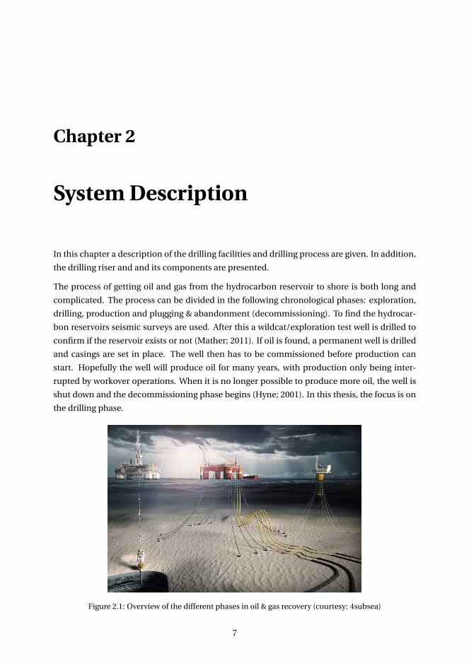
The process of getting oil and gas from the hydrocarbon reservoir to shore is both long and
complicated. The process can be divided in the following chronological phases: exploration,
drilling, production and plugging & abandonment (decommissioning). To find the hydrocar-
bon reservoirs seismic surveys are used. After this a wildcat/exploration test well is drilled to
confirm if the reservoir exists or not (Mather; 2011). If oil is found, a permanent well is drilled
and casings are set in place. The well then has to be commissioned before production can
start. Hopefully the well will produce oil for many years, with production only being inter-
rupted by workover operations. When it is no longer possible to produce more oil, the well is
shut down and the decommissioning phase begins (Hyne; 2001). In this thesis, the focus is on
the drilling phase.
Figure 2.1: Overview of the different phases in oil & gas recovery (courtesy: 4subsea)
7
8 CHAPTER 2. SYSTEM DESCRIPTION
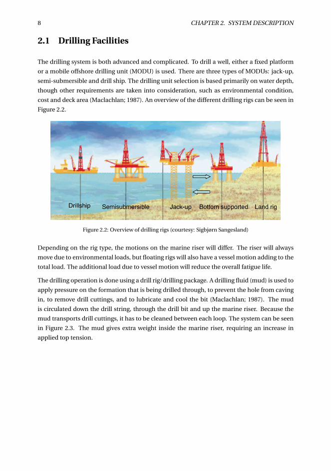
2.1 Drilling Facilities
The drilling system is both advanced and complicated. To drill a well, either a fixed platform
or a mobile offshore drilling unit (MODU) is used. There are three types of MODUs: jack-up,
semi-submersible and drill ship. The drilling unit selection is based primarily on water depth,
though other requirements are taken into consideration, such as environmental condition,
cost and deck area (Maclachlan; 1987). An overview of the different drilling rigs can be seen in
Figure 2.2.
Figure 2.2: Overview of drilling rigs (courtesy: Sigbjørn Sangesland)
Depending on the rig type, the motions on the marine riser will differ. The riser will always
move due to environmental loads, but floating rigs will also have a vessel motion adding to the
total load. The additional load due to vessel motion will reduce the overall fatigue life.
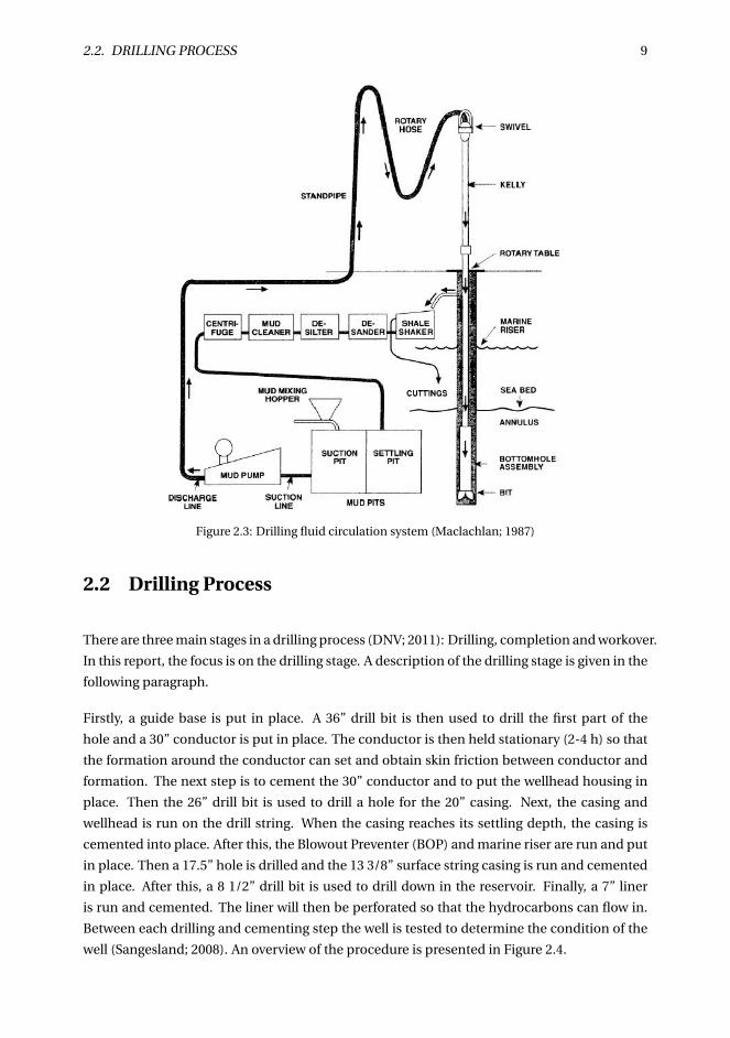
The drilling operation is done using a drill rig/drilling package. A drilling fluid (mud) is used to
apply pressure on the formation that is being drilled through, to prevent the hole from caving
in, to remove drill cuttings, and to lubricate and cool the bit (Maclachlan; 1987). The mud
is circulated down the drill string, through the drill bit and up the marine riser. Because the
mud transports drill cuttings, it has to be cleaned between each loop. The system can be seen
in Figure 2.3. The mud gives extra weight inside the marine riser, requiring an increase in
applied top tension.
2.2. DRILLING PROCESS 9
Figure 2.3: Drilling fluid circulation system (Maclachlan; 1987)
2.2 Drilling Process
There are three main stages in a drilling process (DNV; 2011): Drilling, completion and workover.
In this report, the focus is on the drilling stage. A description of the drilling stage is given in the
following paragraph.
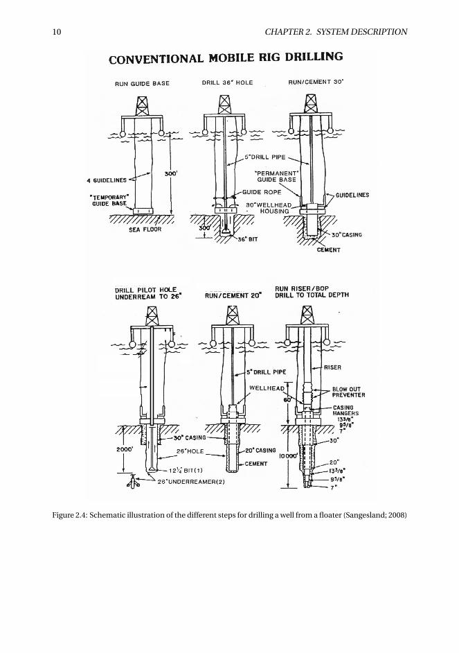
Firstly, a guide base is put in place. A 36” drill bit is then used to drill the first part of the
hole and a 30” conductor is put in place. The conductor is then held stationary (2-4 h) so that
the formation around the conductor can set and obtain skin friction between conductor and
formation. The next step is to cement the 30” conductor and to put the wellhead housing in
place. Then the 26” drill bit is used to drill a hole for the 20” casing. Next, the casing and
wellhead is run on the drill string. When the casing reaches its settling depth, the casing is
cemented into place. After this, the Blowout Preventer (BOP) and marine riser are run and put
in place. Then a 17.5” hole is drilled and the 13 3/8” surface string casing is run and cemented
in place. After this, a 8 1/2” drill bit is used to drill down in the reservoir. Finally, a 7” liner
is run and cemented. The liner will then be perforated so that the hydrocarbons can flow in.
Between each drilling and cementing step the well is tested to determine the condition of the
well (Sangesland; 2008). An overview of the procedure is presented in Figure 2.4.
10 CHAPTER 2. SYSTEM DESCRIPTION
6
Figure 1.2 Schematic illustration of the different steps for drilling a well from a floater
Figure 2.4: Schematic illustration of the different steps for drilling a well from a floater (Sangesland; 2008)
2.3. RISER TYPES 11
2.3 Riser Types
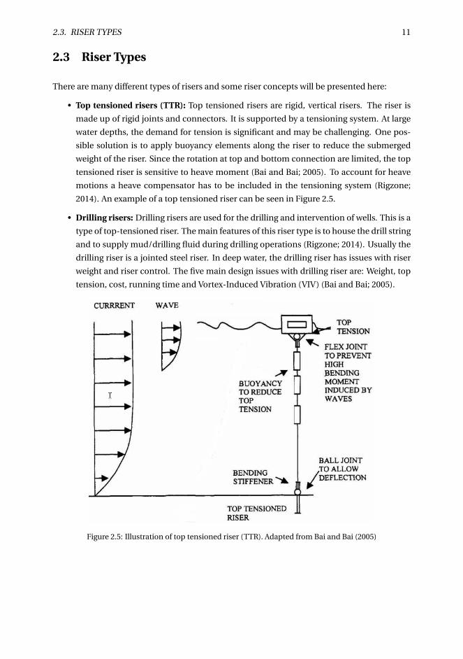
There are many different types of risers and some riser concepts will be presented here:
• Top tensioned risers (TTR): Top tensioned risers are rigid, vertical risers. The riser is
made up of rigid joints and connectors. It is supported by a tensioning system. At large
water depths, the demand for tension is significant and may be challenging. One pos-
sible solution is to apply buoyancy elements along the riser to reduce the submerged
weight of the riser. Since the rotation at top and bottom connection are limited, the top
tensioned riser is sensitive to heave moment (Bai and Bai; 2005). To account for heave
motions a heave compensator has to be included in the tensioning system (Rigzone;
2014). An example of a top tensioned riser can be seen in Figure 2.5.
• Drilling risers: Drilling risers are used for the drilling and intervention of wells. This is a
type of top-tensioned riser. The main features of this riser type is to house the drill string
and to supply mud/drilling fluid during drilling operations (Rigzone; 2014). Usually the
drilling riser is a jointed steel riser. In deep water, the drilling riser has issues with riser
weight and riser control. The five main design issues with drilling riser are: Weight, top
tension, cost, running time and Vortex-Induced Vibration (VIV) (Bai and Bai; 2005).
Figure 2.5: Illustration of top tensioned riser (TTR). Adapted from Bai and Bai (2005)
12 CHAPTER 2. SYSTEM DESCRIPTION
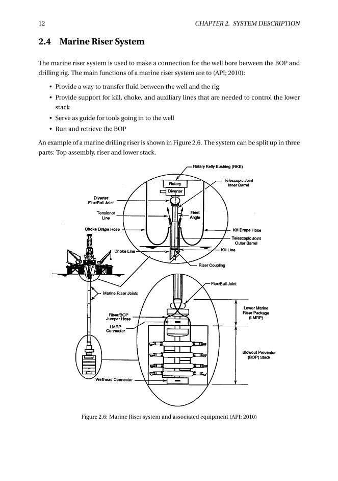
2.4 Marine Riser System
The marine riser system is used to make a connection for the well bore between the BOP and
drilling rig. The main functions of a marine riser system are to (API; 2010):
• Provide a way to transfer fluid between the well and the rig
• Provide support for kill, choke, and auxiliary lines that are needed to control the lower
stack
• Serve as guide for tools going in to the well
• Run and retrieve the BOP
An example of a marine drilling riser is shown in Figure 2.6. The system can be split up in three
parts: Top assembly, riser and lower stack.
Figure 2.6: Marine Riser system and associated equipment (API; 2010)
2.4. MARINE RISER SYSTEM 13
2.4.1 Top Assembly
The top assembly contains the parts where the riser interfaces with the rig.
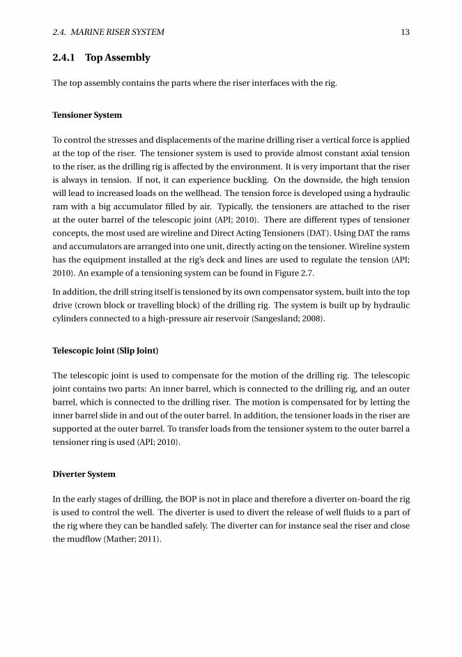
Tensioner System
To control the stresses and displacements of the marine drilling riser a vertical force is applied
at the top of the riser. The tensioner system is used to provide almost constant axial tension
to the riser, as the drilling rig is affected by the environment. It is very important that the riser
is always in tension. If not, it can experience buckling. On the downside, the high tension
will lead to increased loads on the wellhead. The tension force is developed using a hydraulic
ram with a big accumulator filled by air. Typically, the tensioners are attached to the riser
at the outer barrel of the telescopic joint (API; 2010). There are different types of tensioner
concepts, the most used are wireline and Direct Acting Tensioners (DAT). Using DAT the rams
and accumulators are arranged into one unit, directly acting on the tensioner. Wireline system
has the equipment installed at the rig’s deck and lines are used to regulate the tension (API;
2010). An example of a tensioning system can be found in Figure 2.7.
In addition, the drill string itself is tensioned by its own compensator system, built into the top
drive (crown block or travelling block) of the drilling rig. The system is built up by hydraulic
cylinders connected to a high-pressure air reservoir (Sangesland; 2008).
Telescopic Joint (Slip Joint)
The telescopic joint is used to compensate for the motion of the drilling rig. The telescopic
joint contains two parts: An inner barrel, which is connected to the drilling rig, and an outer
barrel, which is connected to the drilling riser. The motion is compensated for by letting the
inner barrel slide in and out of the outer barrel. In addition, the tensioner loads in the riser are
supported at the outer barrel. To transfer loads from the tensioner system to the outer barrel a
tensioner ring is used (API; 2010).
Diverter System
In the early stages of drilling, the BOP is not in place and therefore a diverter on-board the rig
is used to control the well. The diverter is used to divert the release of well fluids to a part of
the rig where they can be handled safely. The diverter can for instance seal the riser and close
the mudflow (Mather; 2011).
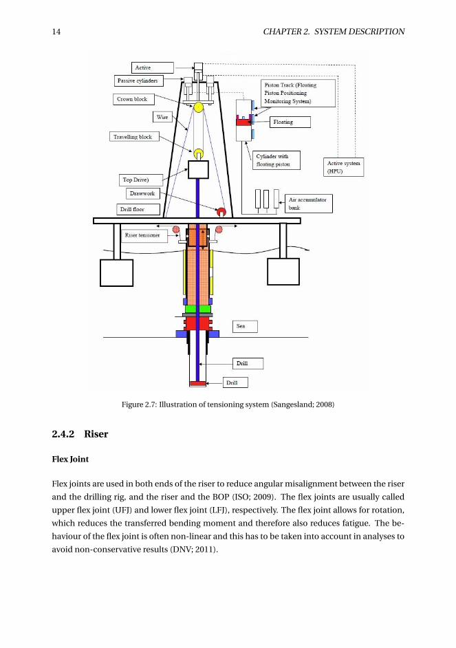
14 CHAPTER 2. SYSTEM DESCRIPTION
Figure 2.7: Illustration of tensioning system (Sangesland; 2008)
2.4.2 Riser
Flex Joint
Flex joints are used in both ends of the riser to reduce angular misalignment between the riser
and the drilling rig, and the riser and the BOP (ISO; 2009). The flex joints are usually called
upper flex joint (UFJ) and lower flex joint (LFJ), respectively. The flex joint allows for rotation,
which reduces the transferred bending moment and therefore also reduces fatigue. The be-
haviour of the flex joint is often non-linear and this has to be taken into account in analyses to
avoid non-conservative results (DNV; 2011).
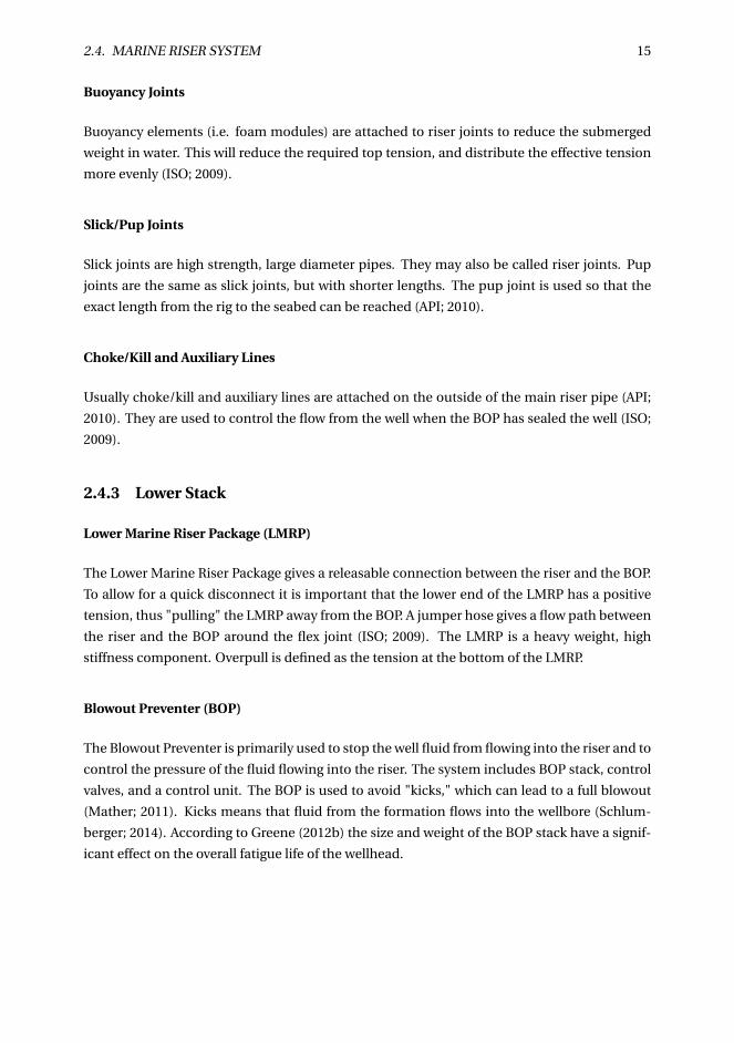
2.4. MARINE RISER SYSTEM 15
Buoyancy Joints
Buoyancy elements (i.e. foam modules) are attached to riser joints to reduce the submerged
weight in water. This will reduce the required top tension, and distribute the effective tension
more evenly (ISO; 2009).
Slick/Pup Joints
Slick joints are high strength, large diameter pipes. They may also be called riser joints. Pup
joints are the same as slick joints, but with shorter lengths. The pup joint is used so that the
exact length from the rig to the seabed can be reached (API; 2010).
Choke/Kill and Auxiliary Lines
Usually choke/kill and auxiliary lines are attached on the outside of the main riser pipe (API;
2010). They are used to control the flow from the well when the BOP has sealed the well (ISO;
2009).
2.4.3 Lower Stack
Lower Marine Riser Package (LMRP)
The Lower Marine Riser Package gives a releasable connection between the riser and the BOP.
To allow for a quick disconnect it is important that the lower end of the LMRP has a positive
tension, thus "pulling" the LMRP away from the BOP. A jumper hose gives a flow path between
the riser and the BOP around the flex joint (ISO; 2009). The LMRP is a heavy weight, high
stiffness component. Overpull is defined as the tension at the bottom of the LMRP.
Blowout Preventer (BOP)
The Blowout Preventer is primarily used to stop the well fluid from flowing into the riser and to
control the pressure of the fluid flowing into the riser. The system includes BOP stack, control
valves, and a control unit. The BOP is used to avoid "kicks," which can lead to a full blowout
(Mather; 2011). Kicks means that fluid from the formation flows into the wellbore (Schlum-
berger; 2014). According to Greene (2012b) the size and weight of the BOP stack have a signif-
icant effect on the overall fatigue life of the wellhead.
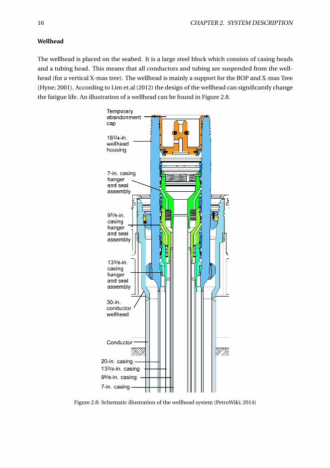
16 CHAPTER 2. SYSTEM DESCRIPTION
Wellhead
The wellhead is placed on the seabed. It is a large steel block which consists of casing heads
and a tubing head. This means that all conductors and tubing are suspended from the well-
head (for a vertical X-mas tree). The wellhead is mainly a support for the BOP and X-mas Tree
(Hyne; 2001). According to Lim et.al (2012) the design of the wellhead can significantly change
the fatigue life. An illustration of a wellhead can be found in Figure 2.8.
Figure 2.8: Schematic illustration of the wellhead system (PetroWiki; 2014)

Chapter 3
Dynamic Theory
This chapter presents theories related to global load analysis, some of which that SIMA/RI-
FLEX is based on. An introduction to finite element method will be presented, in addition to
tension calculation, static analysis, eigenvalue analysis, hydrodynamic loads, stochastic the-
ory and time domain analysis.
3.1 Finite Element Model
For a dynamic analysis the equilibrium equation is written (Langen and Sigbjörnsson; 1979):
Mv +Cv +Kv = Q(t) (3.1)
where:
M Mass Matrix
C Damping Matrix
K Stiffness Matrix
Q External Load Vector
v , v , v Displacement, Velocity and Acceleration Vector
To model risers, beam elements are typically used. An example of a linear 2D beam element
and its degrees of freedom can be found in Figure 3.1.
17
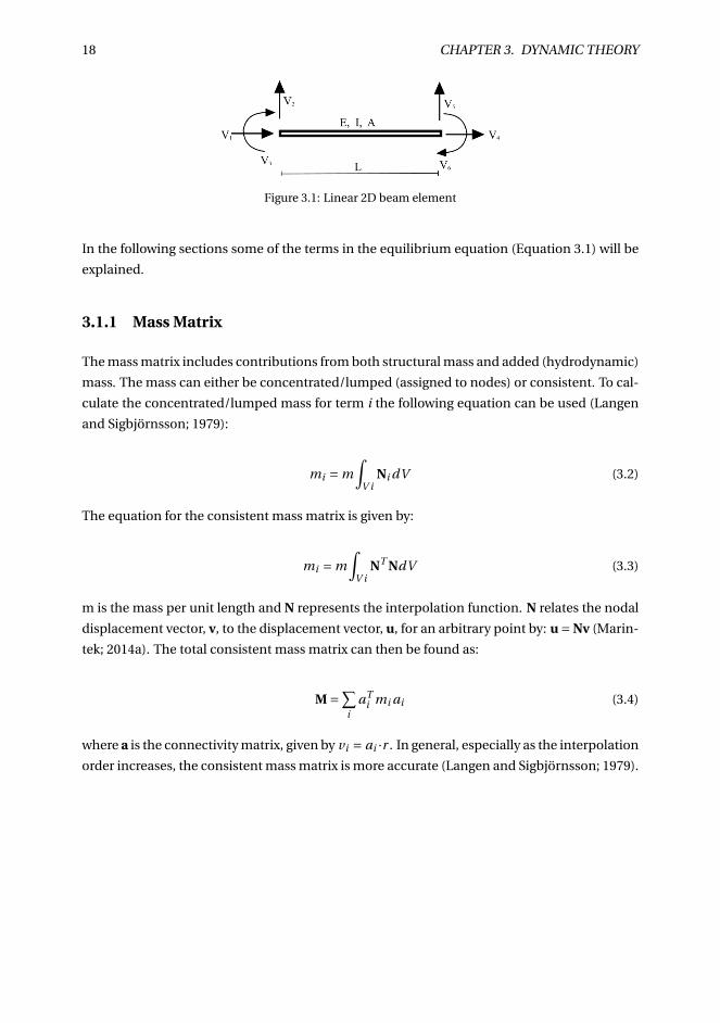
18 CHAPTER 3. DYNAMIC THEORY
Figure 3.1: Linear 2D beam element
In the following sections some of the terms in the equilibrium equation (Equation 3.1) will be
explained.
3.1.1 Mass Matrix
The mass matrix includes contributions from both structural mass and added (hydrodynamic)
mass. The mass can either be concentrated/lumped (assigned to nodes) or consistent. To cal-
culate the concentrated/lumped mass for term i the following equation can be used (Langen
and Sigbjörnsson; 1979):
mi = m∫
V iNi dV (3.2)
The equation for the consistent mass matrix is given by:
mi = m∫
V iNT NdV (3.3)
m is the mass per unit length and N represents the interpolation function. N relates the nodal
displacement vector, v, to the displacement vector, u, for an arbitrary point by: u = Nv (Marin-
tek; 2014a). The total consistent mass matrix can then be found as:
M =∑i
aTi mi ai (3.4)
where a is the connectivity matrix, given by vi = ai ·r . In general, especially as the interpolation
order increases, the consistent mass matrix is more accurate (Langen and Sigbjörnsson; 1979).

3.1. FINITE ELEMENT MODEL 19
3.1.2 Stiffness Matrix
For a beam element, if shear deformations are neglected, the stiffness matrix for the 6 degree
of freedom element can be derived from Euler-Bernoulli beam theory. The stiffness matrix
becomes (Langen and Sigbjörnsson; 1979):
kE =
E Al 0 0 −E A
l 0 0
0 12E Il 3
−6E Il
−12E Il 3
6E Il 2
0 −6E Il 2
4E Il 0 6E I
l 22E I
l−E A
l 0 0 E Al 0 0
0 −12E Il 3
6E Il 2 0 12E I
l 36E Il 2
0 −6E Il 2
2E Il 0 6E I
l 24E I
l
(3.5)
Using non-linear theory, there will also be a contribution from geometric stiffness in the global
stiffness matrix. This can be seen from the equation for strain, which includes a second-order
term (Moan; 2003).
εx = u,x − z ∗w,xx + 1
2w2
,x (3.6)
The geometric stiffness matrix (if the terms are linearised) is given by (Gavin; 2012):
kG =
0 0 0 0 0 0
0 6P5l
−P10 0 −6P
5l−P10
0 −P10
2Pl15 0 P
10−Pl30
0 0 0 0 0 0
0 −6P5l
P10 0 6P
5lP10
0 −P10
−Pl30 0 P
102Pl15
(3.7)
Where P is the axial force in the element.
Combining the elastic and geometric stiffness gives the total stiffness matrix for element i:
ki = kE ,i +kG ,i (3.8)
Then the total system stiffness matrix becomes (Langen and Sigbjörnsson; 1979):
K =∑i
aTi T T
i ki Ti ai (3.9)
where a is the connectivity matrix and T is the transformation matrix. a and T are used to
transform the local stiffness matrix into the global system matrix.
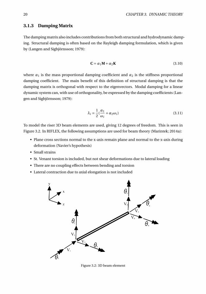
20 CHAPTER 3. DYNAMIC THEORY
3.1.3 Damping Matrix
The damping matrix also includes contributions from both structural and hydrodynamic damp-
ing. Structural damping is often based on the Rayleigh damping formulation, which is given
by (Langen and Sigbjörnsson; 1979):
C =α1M+α2K (3.10)
where α1 is the mass proportional damping coefficient and α2 is the stiffness proportional
damping coefficient. The main benefit of this definition of structural damping is that the
damping matrix is orthogonal with respect to the eigenvectors. Modal damping for a linear
dynamic system can, with use of orthogonality, be expressed by the damping coefficients (Lan-
gen and Sigbjörnsson; 1979):
λi = 1
2(α1
ωi+α2ωi ) (3.11)
To model the riser 3D beam elements are used, giving 12 degrees of freedom. This is seen in
Figure 3.2. In RIFLEX, the following assumptions are used for beam theory (Marintek; 2014a):
• Plane cross sections normal to the x-axis remain plane and normal to the x-axis during
deformation (Navier’s hypothesis)
• Small strains
• St. Venant torsion is included, but not shear deformations due to lateral loading
• There are no coupling effects between bending and torsion
• Lateral contraction due to axial elongation is not included
Figure 3.2: 3D beam element
3.2. STATIC ANALYSIS 21
3.2 Static Analysis
To ensure that the system is in static equilibrium a static analysis is conducted to obtain the
nodal displacements. The equation can be given as (Moan; 2003):
K(r)r = R (3.12)
where r is the nodal displacement vector, K(r) the internal structural reaction force vector, and
R the external force vector. It can also be given on differential form (Moan; 2003):
d
dr(K(r))r)︸ ︷︷ ︸KI (r )
dr = dR (3.13)
Where KI (r) is the tangential stiffness (incremental stiffness) given as a combination of mate-
rial (KM ), geometry (KG ) and external (KE ) stiffness matrices (Moan; 2003):
KI = KM +KG +KE (3.14)
As the problem is non-linear, a numerical procedure has to be used to solve the problem. Non-
linear problems do not necessarily have a unique solution, unlike linear problems. Therefore,
the obtained solution may not be the one wished for (Moan; 2003). There are in general three
types of solution procedures: incremental, iterative, and combined methods (Moan; 2003). In
RIFLEX a incremental-iterative procedure with Euler-Cauchy incrementation is used (Marin-
tek; 2014a).
An incremental method applies the external loading stepwise and sums up the displacement
increments to obtain the total displacement. For the Euler-Cauchy method, the difference in
force at each load step is given as (Marintek; 2014a):
∆R = KI∆r (3.15)
The following equations are used to calculate a load increment for loadstep m+1 (Moan; 2003):
∆Rm+1 = Rm+1 −Rm (3.16)
∆rm+1 = KI (rm)−1∆Rm+1 (3.17)
rm+1 = rm +∆rm+1 (3.18)
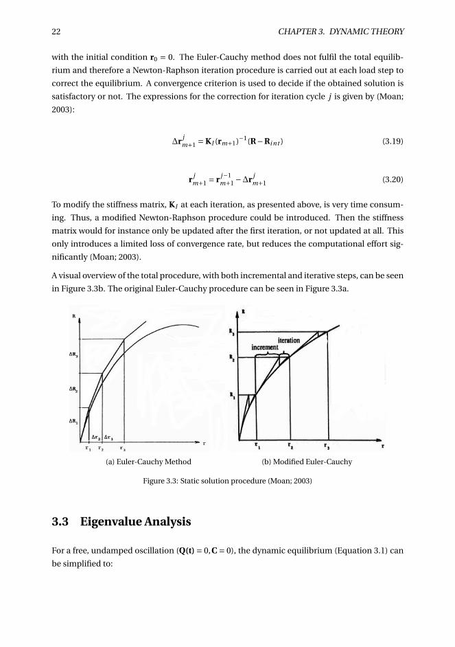
22 CHAPTER 3. DYNAMIC THEORY
with the initial condition r0 = 0. The Euler-Cauchy method does not fulfil the total equilib-
rium and therefore a Newton-Raphson iteration procedure is carried out at each load step to
correct the equilibrium. A convergence criterion is used to decide if the obtained solution is
satisfactory or not. The expressions for the correction for iteration cycle j is given by (Moan;
2003):
∆r jm+1 = KI (rm+1)−1(R−Ri nt ) (3.19)
r jm+1 = r j−1
m+1 −∆r jm+1 (3.20)
To modify the stiffness matrix, KI at each iteration, as presented above, is very time consum-
ing. Thus, a modified Newton-Raphson procedure could be introduced. Then the stiffness
matrix would for instance only be updated after the first iteration, or not updated at all. This
only introduces a limited loss of convergence rate, but reduces the computational effort sig-
nificantly (Moan; 2003).
A visual overview of the total procedure, with both incremental and iterative steps, can be seen
in Figure 3.3b. The original Euler-Cauchy procedure can be seen in Figure 3.3a.
(a) Euler-Cauchy Method (b) Modified Euler-Cauchy
Figure 3.3: Static solution procedure (Moan; 2003)
3.3 Eigenvalue Analysis
For a free, undamped oscillation (Q(t) = 0,C = 0), the dynamic equilibrium (Equation 3.1) can
be simplified to:
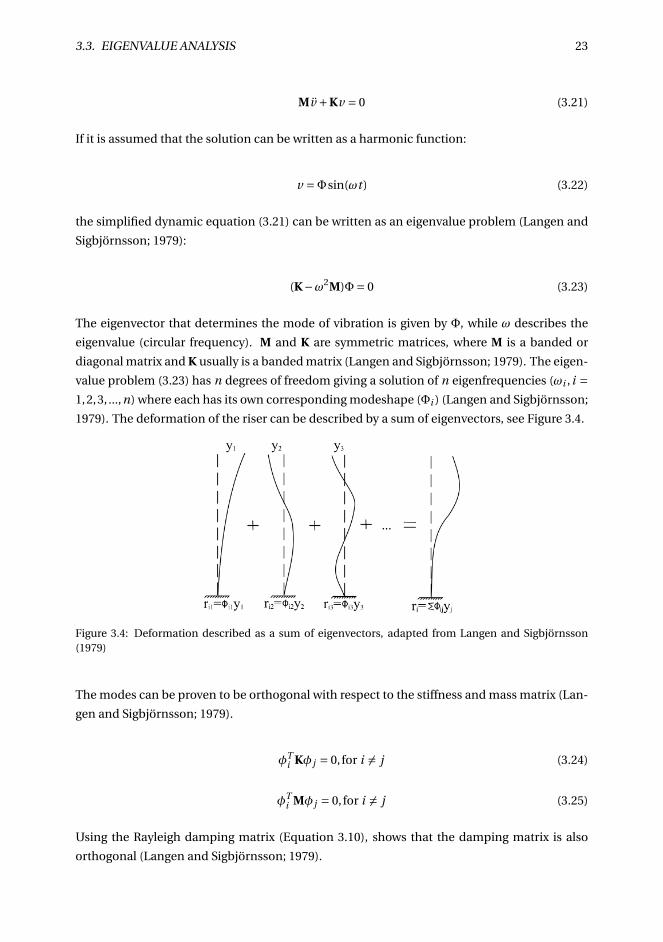
3.3. EIGENVALUE ANALYSIS 23
Mv +Kv = 0 (3.21)
If it is assumed that the solution can be written as a harmonic function:
v =Φsin(ωt ) (3.22)
the simplified dynamic equation (3.21) can be written as an eigenvalue problem (Langen and
Sigbjörnsson; 1979):
(K−ω2M)Φ= 0 (3.23)
The eigenvector that determines the mode of vibration is given by Φ, while ω describes the
eigenvalue (circular frequency). M and K are symmetric matrices, where M is a banded or
diagonal matrix and K usually is a banded matrix (Langen and Sigbjörnsson; 1979). The eigen-
value problem (3.23) has n degrees of freedom giving a solution of n eigenfrequencies (ωi , i =1,2,3, ...,n) where each has its own corresponding modeshape (Φi ) (Langen and Sigbjörnsson;
1979). The deformation of the riser can be described by a sum of eigenvectors, see Figure 3.4.
Figure 3.4: Deformation described as a sum of eigenvectors, adapted from Langen and Sigbjörnsson(1979)
The modes can be proven to be orthogonal with respect to the stiffness and mass matrix (Lan-
gen and Sigbjörnsson; 1979).
φTi Kφ j = 0,for i 6= j (3.24)
φTi Mφ j = 0,for i 6= j (3.25)
Using the Rayleigh damping matrix (Equation 3.10), shows that the damping matrix is also
orthogonal (Langen and Sigbjörnsson; 1979).
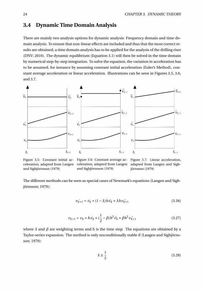
24 CHAPTER 3. DYNAMIC THEORY
3.4 Dynamic Time Domain Analysis
There are mainly two analysis options for dynamic analysis: Frequency domain and time do-
main analysis. To ensure that non-linear effects are included and thus that the most correct re-
sults are obtained, a time domain analysis has to be applied for the analysis of the drilling riser
(DNV; 2010). The dynamic equilibrium (Equation 3.1) will then be solved in the time domain
by numerical step-by-step integration. To solve the equation, the variation in acceleration has
to be assumed, for instance by assuming constant initial acceleration (Euler’s Method), con-
stant average acceleration or linear acceleration. Illustrations can be seen in Figures 3.5, 3.6,
and 3.7.
Figure 3.5: Constant initial ac-celeration, adapted from Langenand Sigbjörnsson (1979)
Figure 3.6: Constant average ac-celeration, adapted from Langenand Sigbjörnsson (1979)
Figure 3.7: Linear acceleration,adapted from Langen and Sigb-jörnsson (1979)
The different methods can be seen as special cases of Newmark’s equations (Langen and Sigb-
jörnsson; 1979):
˙vk+1 = vk + (1−λ)hvk +λh ¨vk+1 (3.26)
vk+1 = vk +hvk + (1
2−β)h2vk +βh2 ¨vk+1 (3.27)
where λ and β are weighting terms and h is the time step. The equations are obtained by a
Taylor-series expansion. The method is only unconditionally stable if (Langen and Sigbjörns-
son; 1979):
λ≥ 1
2(3.28)
3.5. EFFECTIVE TENSION 25
β≥ 1
4(λ+ 1
2)2 (3.29)
λ decides the artificial damping. To avoid artificial damping λ must be equal to 12 . β depends
on the type of method, for instance for linear acceleration β = 16 (Langen and Sigbjörnsson;
1979).
3.5 Effective Tension
The effective tension can be defined as the axial force in the wall including the contributions
from internal and external pressure. The effective tension can be calculated (DNV; 2010):
Te = Tw −pi Ai +pe Ae (3.30)
where
Te Effective tension
Tw True wall tension
pi , pe Internal- and external (local) pressure
Ai , Ae Internal- and external cross section area
If the effective tension is negative, the drilling riser might buckle. It buckles as a beam-column
in compression. To avoid compressive effective tension in the riser for a static position, a lower
limit for tension is introduced. The lower limit is defined by the effective weight of the system.
The effective weight can be calculated as (DNV; 2010):
We = Mp g + Aiρi g − Aeρe g (3.31)
where
Mp Mass of pipe
g Acceleration of gravity
ρi , ρe Internal- and external fluid density
Ai , Ae Internal- and external cross section area
The applied top tension is therefore given as the effective weight, in addition to an overpull.
The combined weight is converted to a force and applied at the top of the riser (tensioner ring
node):
Ttop = (We +overpull) · g (3.32)
26 CHAPTER 3. DYNAMIC THEORY
3.6 Hydrodynamic Loads
To calculate the loads on the riser, Morison’s equation is used. In this form of the equation the
horizontal movement of the riser is also included to give the most accurate result (DNV; 2010).
dF = 1
2ρCD Dh |u − x| (u − x)+ρπD2
b
4CM a −ρπD2
b
4(CM −1)x (3.33)
where
dF Force per unit length
ρ Water density
CM ,CD Inertia- and Drag Coefficient
Db ,Dh Buoyancy- and Hydrodynamic diameter
u,a Velocity- and Acceleration of water particle
x,x Velocity- and Acceleration of structure
The two first terms of Morison’s equation are included as an external load, while the last term,
which includes the added mass (C A =CM −1), is included in the mass matrix. Hence, this term
affects the eigenmodes and eigenperiods of the riser (DNV; 2010).
If regular waves and deep water is assumed, the wave potential can be written as (Faltinsen;
1998):
φ= gζa
ωekz cos(ωt −kx) (3.34)
where ζa is the wave amplitude and k is the wave number (ω2 = kg ). The particle speed and
acceleration are defined by:
u = ∂φ∂x a = ∂u
∂t
Introducing this into Equation 3.33 shows that the inertia term varies with cos(x) and the drag
term with sin(x) |sin(x)|. A visualisation can be seen in Figure 3.8.
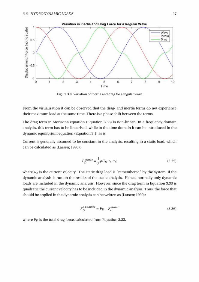
3.6. HYDRODYNAMIC LOADS 27
Figure 3.8: Variation of inertia and drag for a regular wave
From the visualisation it can be observed that the drag- and inertia terms do not experience
their maximum load at the same time. There is a phase shift between the terms.
The drag term in Morison’s equation (Equation 3.33) is non-linear. In a frequency domain
analysis, this term has to be linearised, while in the time domain it can be introduced in the
dynamic equilibrium equation (Equation 3.1) as is.
Current is generally assumed to be constant in the analysis, resulting in a static load, which
can be calculated as (Larsen; 1990):
F st ati cD = 1
2ρCD uc |uc | (3.35)
where uc is the current velocity. The static drag load is "remembered" by the system, if the
dynamic analysis is run on the results of the static analysis. Hence, normally only dynamic
loads are included in the dynamic analysis. However, since the drag term in Equation 3.33 is
quadratic the current velocity has to be included in the dynamic analysis. Thus, the force that
should be applied in the dynamic analysis can be written as (Larsen; 1990):
F d ynami cD = FD −F st ati c
D (3.36)
where FD is the total drag force, calculated from Equation 3.33.
28 CHAPTER 3. DYNAMIC THEORY
3.7 Stochastic Theory
Stochastic theory is used to describe the wave process. The wave process is uncertain, as it is
not known exactly what will happen in the future. Hence, statistics are used to predict results.
The process is stationary if the statistical properties do not change over time. It is common to
assume that the wave elevation is stationary for a time interval of 3-6 hours (Almar-Næss et al.;
1985).
The wave elevation in an irregular sea can be written as a sum of regular waves, with different
directions, wave lengths, and amplitudes (Faltinsen; 1998):
ζ(t ) =N∑
i=1ζa,i sin(ωi t −ki x +ε j ) (3.37)
ε j is a random phase angle, which is uniformly distributed in the interval (0,2π). ζa,i is the
wave amplitude and is expressed by the wave spectrum:
1
2ζ2
a,i = S(ωi )∆ω (3.38)
A general definition of the wave spectrum, S(ω), for a Gaussian process with zero mean is
defined as (Newland; 1993):
S(ω) = 1
2π
∫ ∞
−∞R(τ)e−iωτdτ (3.39)
where R(τ) is the autocorrelation function.
For the North Sea, it is common to use the JONSWAP spectrum, which is defined as (Marintek;
2014b):
S(ω) =αg 2ω−5exp(−1.25(ωp
ω)4)γ
exp(− (ω−ωp )2
2σ2ω2p
)(3.40)
where α is given as:
α= 1.2905H 2
s
T 4z
(3.41)
and the relation between Tp and Tz is as follows:
Tp
Tz= 1.407(1−0.287lnγ)
14 (3.42)
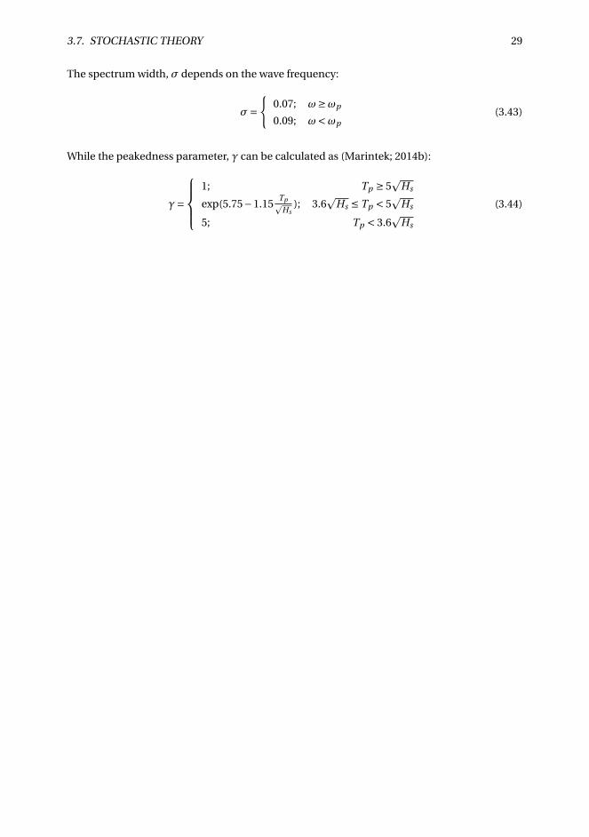
3.7. STOCHASTIC THEORY 29
The spectrum width, σ depends on the wave frequency:
σ={
0.07; ω≥ωp
0.09; ω<ωp(3.43)
While the peakedness parameter, γ can be calculated as (Marintek; 2014b):
γ=
1; Tp ≥ 5
pHs
exp(5.75−1.15TppHs
); 3.6p
Hs ≤ Tp < 5p
Hs
5; Tp < 3.6p
Hs
(3.44)


Chapter 4
Fatigue Theory
In this chapter the theory related to the fatigue calculations are presented. This includes pre-
sentations of load history, development of SN-curves, procedures for cycle counting, applica-
tion of histograms, and Miner-Palmgren summation.
4.1 Fatigue Damage
Cyclic loads, where the loads are normally smaller than the yield stress of the material, cause
fatigue. Abrupt failure will thus not occur, but every cycle will accumulate damage ultimately
leading to failure. The fatigue history can be divided into three stages (Berge; 2006):
• Initiation
• Crack growth
• Final failure
Generally, crack initiation is the domineering phase for smooth, un-welded components. Welded
components have initial flaws, and crack growth is therefore the domineering phase (DNV;
2011). Depending on the phase, the fatigue damage process is governed by different stresses.
Crack initiation is governed by yield stress, and von Mises stress is therefore applied, while for
crack growth the largest cyclic stress is applied (DNV; 2011). For the wellhead system, the flaws
(cracks) are usually present from manufacturing, and cyclic loading leads to crack growth and
ultimately failure. Wellhead failure can be indicated by loss of pressure containment or loss of
structural integrity (Evans and McGrail; 2011). Crack growth is described by the crack prop-
agation rate, da/dN, where da is the change in crack length and dN the change in number of
cycles. The crack growth can be divided into 3 regions: Threshold (A), intermediate (B), and
failure (C) (Almar-Næss et al.; 1985). The crack growth curve can be seen in Figure 4.1.
31
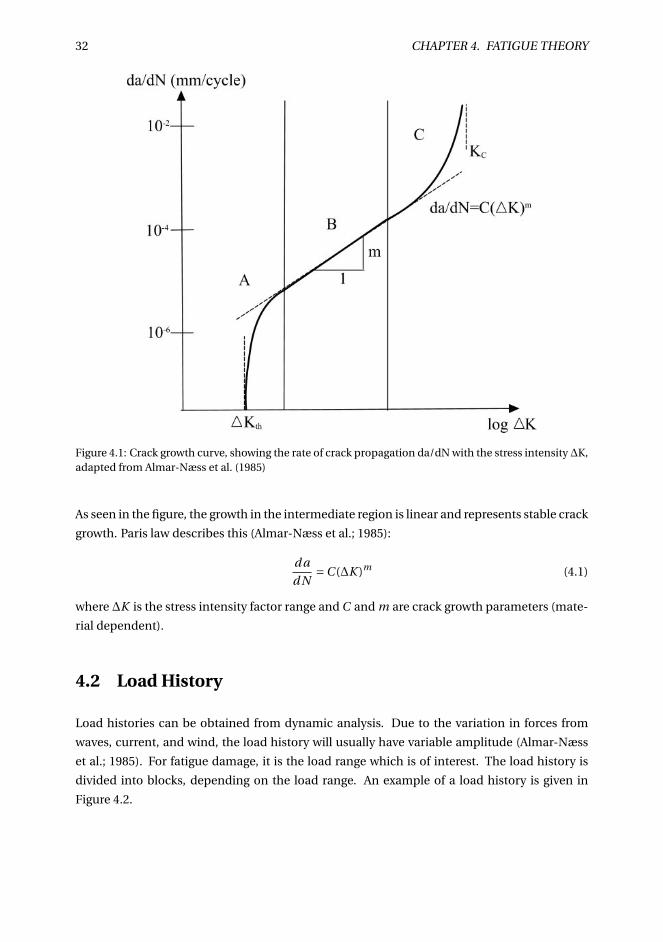
32 CHAPTER 4. FATIGUE THEORY
Figure 4.1: Crack growth curve, showing the rate of crack propagation da/dN with the stress intensity∆K,adapted from Almar-Næss et al. (1985)
As seen in the figure, the growth in the intermediate region is linear and represents stable crack
growth. Paris law describes this (Almar-Næss et al.; 1985):
d a
d N=C (∆K )m (4.1)
where ∆K is the stress intensity factor range and C and m are crack growth parameters (mate-
rial dependent).
4.2 Load History
Load histories can be obtained from dynamic analysis. Due to the variation in forces from
waves, current, and wind, the load history will usually have variable amplitude (Almar-Næss
et al.; 1985). For fatigue damage, it is the load range which is of interest. The load history is
divided into blocks, depending on the load range. An example of a load history is given in
Figure 4.2.
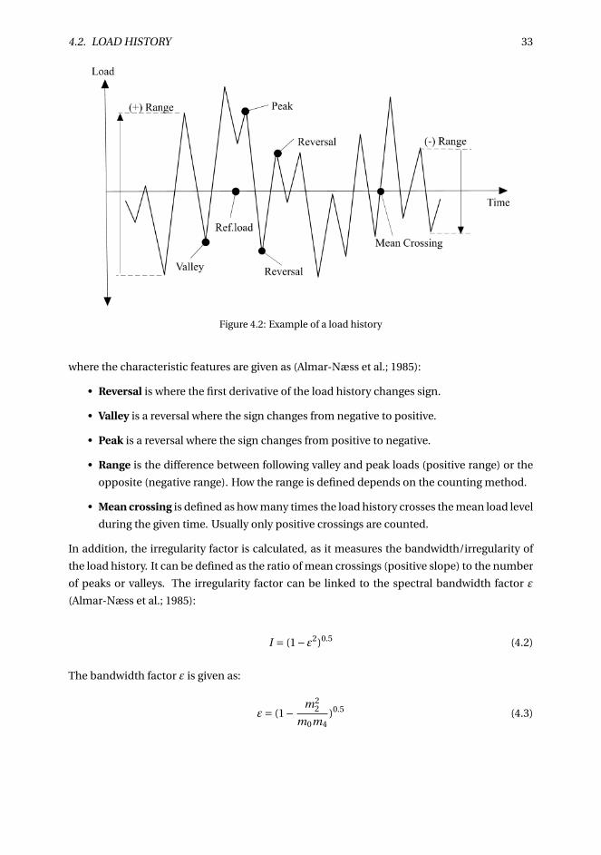
4.2. LOAD HISTORY 33
Figure 4.2: Example of a load history
where the characteristic features are given as (Almar-Næss et al.; 1985):
• Reversal is where the first derivative of the load history changes sign.
• Valley is a reversal where the sign changes from negative to positive.
• Peak is a reversal where the sign changes from positive to negative.
• Range is the difference between following valley and peak loads (positive range) or the
opposite (negative range). How the range is defined depends on the counting method.
• Mean crossing is defined as how many times the load history crosses the mean load level
during the given time. Usually only positive crossings are counted.
In addition, the irregularity factor is calculated, as it measures the bandwidth/irregularity of
the load history. It can be defined as the ratio of mean crossings (positive slope) to the number
of peaks or valleys. The irregularity factor can be linked to the spectral bandwidth factor ε
(Almar-Næss et al.; 1985):
I = (1−ε2)0.5 (4.2)
The bandwidth factor ε is given as:
ε= (1− m22
m0m4)0.5 (4.3)
34 CHAPTER 4. FATIGUE THEORY
where mn is the n’th spectral moment obtained from the wave spectrum (Equation 3.39):
mn =∫ ∞
0ωnS(ω)dω (4.4)
For a narrow banded process ε≈ 0.
4.3 S-N Curves
S-N curves (also called Wöhler curves) are used to describe the fatigue properties of a mate-
rial given by the load range as a function of cycles until failure. The curve is obtained from
experimental data and is described by the relationship (Almar-Næss et al.; 1985):
N (∆S)m = a (4.5)
where ∆S is the stress range, N is the number of cycles to failure and m and a are constants.
It is observed that this equation is analogous to Paris law given in Equation 4.1, in the stable
crack growth range. The S-N curve is normally plotted logarithmically, which results in a linear
curve and Equation 4.5 can be rewritten as:
log N = l og a −m · l og (∆S) (4.6)
The SN-curve applied for design is the mean curve minus two standard deviations, given by
(DNV GL; 2014):
log a = log a −2 ·σl og N (4.7)
An example of a S-N curve for a constant amplitude loading can be seen in Figure 4.3. For low
stress ranges, specimens may have "infinite" life. In a S-N curve this is introduced as a fatigue
limit, where it is assumed that no damage occurs below this limit (Berge; 2006).
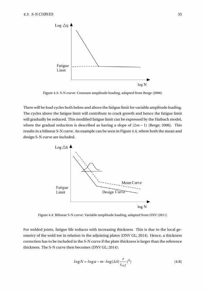
4.3. S-N CURVES 35
Figure 4.3: S-N curve: Constant amplitude loading, adapted from Berge (2006)
There will be load cycles both below and above the fatigue limit for variable amplitude loading.
The cycles above the fatigue limit will contribute to crack growth and hence the fatigue limit
will gradually be reduced. This modified fatigue limit can be expressed by the Haibach model,
where the gradual reduction is described as having a slope of (2m − 1) (Berge; 2006). This
results in a bilinear S-N curve. An example can be seen in Figure 4.4, where both the mean and
design S-N curve are included.
Figure 4.4: Bilinear S-N curve: Variable amplitude loading, adapted from DNV (2011)
For welded joints, fatigue life reduces with increasing thickness. This is due to the local ge-
ometry of the weld toe in relation to the adjoining plates (DNV GL; 2014). Hence, a thickness
correction has to be included in the S-N curve if the plate thickness is larger than the reference
thickness. The S-N curve then becomes (DNV GL; 2014):
log N = l og a −m · l og (∆S(t
tr e f)k ) (4.8)
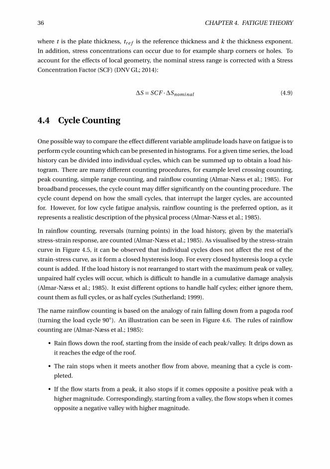
36 CHAPTER 4. FATIGUE THEORY
where t is the plate thickness, tr e f is the reference thickness and k the thickness exponent.
In addition, stress concentrations can occur due to for example sharp corners or holes. To
account for the effects of local geometry, the nominal stress range is corrected with a Stress
Concentration Factor (SCF) (DNV GL; 2014):
∆S = SC F ·∆Snomi nal (4.9)
4.4 Cycle Counting
One possible way to compare the effect different variable amplitude loads have on fatigue is to
perform cycle counting which can be presented in histograms. For a given time series, the load
history can be divided into individual cycles, which can be summed up to obtain a load his-
togram. There are many different counting procedures, for example level crossing counting,
peak counting, simple range counting, and rainflow counting (Almar-Næss et al.; 1985). For
broadband processes, the cycle count may differ significantly on the counting procedure. The
cycle count depend on how the small cycles, that interrupt the larger cycles, are accounted
for. However, for low cycle fatigue analysis, rainflow counting is the preferred option, as it
represents a realistic description of the physical process (Almar-Næss et al.; 1985).
In rainflow counting, reversals (turning points) in the load history, given by the material’s
stress-strain response, are counted (Almar-Næss et al.; 1985). As visualised by the stress-strain
curve in Figure 4.5, it can be observed that individual cycles does not affect the rest of the
strain-stress curve, as it form a closed hysteresis loop. For every closed hysteresis loop a cycle
count is added. If the load history is not rearranged to start with the maximum peak or valley,
unpaired half cycles will occur, which is difficult to handle in a cumulative damage analysis
(Almar-Næss et al.; 1985). It exist different options to handle half cycles; either ignore them,
count them as full cycles, or as half cycles (Sutherland; 1999).
The name rainflow counting is based on the analogy of rain falling down from a pagoda roof
(turning the load cycle 90◦). An illustration can be seen in Figure 4.6. The rules of rainflow
counting are (Almar-Næss et al.; 1985):
• Rain flows down the roof, starting from the inside of each peak/valley. It drips down as
it reaches the edge of the roof.
• The rain stops when it meets another flow from above, meaning that a cycle is com-
pleted.
• If the flow starts from a peak, it also stops if it comes opposite a positive peak with a
higher magnitude. Correspondingly, starting from a valley, the flow stops when it comes
opposite a negative valley with higher magnitude.
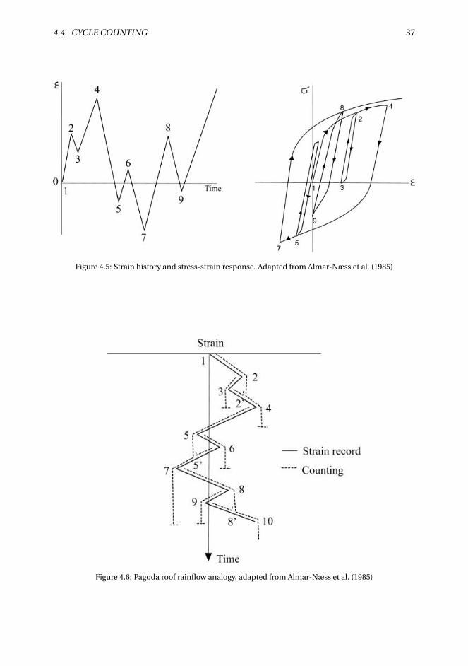
4.4. CYCLE COUNTING 37
Figure 4.5: Strain history and stress-strain response. Adapted from Almar-Næss et al. (1985)
Figure 4.6: Pagoda roof rainflow analogy, adapted from Almar-Næss et al. (1985)
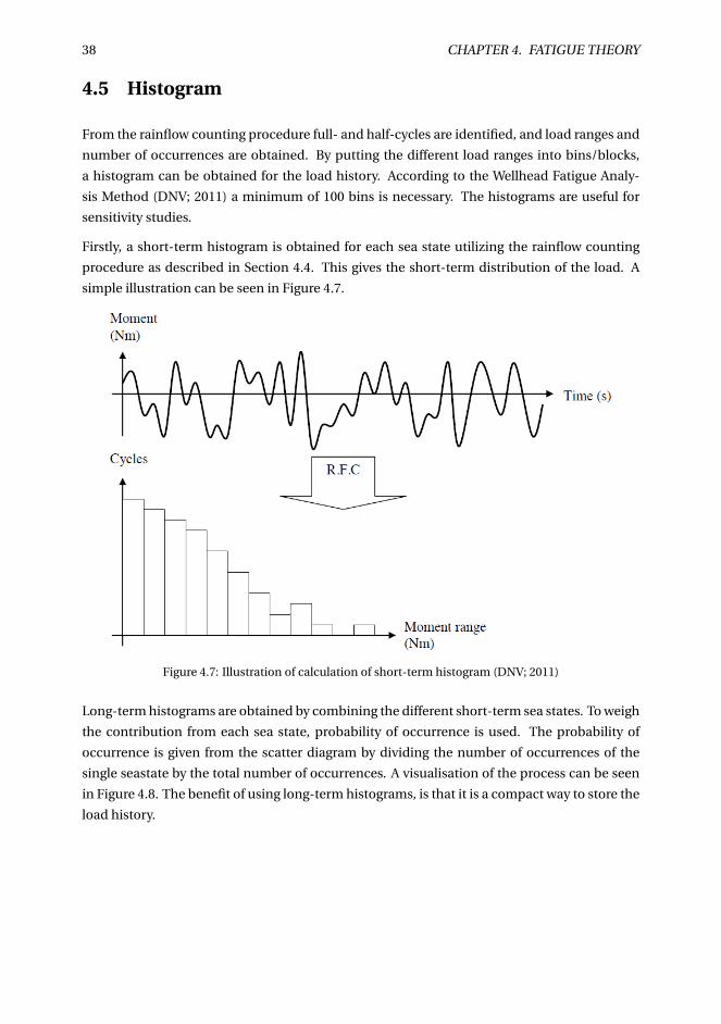
38 CHAPTER 4. FATIGUE THEORY
4.5 Histogram
From the rainflow counting procedure full- and half-cycles are identified, and load ranges and
number of occurrences are obtained. By putting the different load ranges into bins/blocks,
a histogram can be obtained for the load history. According to the Wellhead Fatigue Analy-
sis Method (DNV; 2011) a minimum of 100 bins is necessary. The histograms are useful for
sensitivity studies.
Firstly, a short-term histogram is obtained for each sea state utilizing the rainflow counting
procedure as described in Section 4.4. This gives the short-term distribution of the load. A
simple illustration can be seen in Figure 4.7.
Figure 4.7: Illustration of calculation of short-term histogram (DNV; 2011)
Long-term histograms are obtained by combining the different short-term sea states. To weigh
the contribution from each sea state, probability of occurrence is used. The probability of
occurrence is given from the scatter diagram by dividing the number of occurrences of the
single seastate by the total number of occurrences. A visualisation of the process can be seen
in Figure 4.8. The benefit of using long-term histograms, is that it is a compact way to store the
load history.
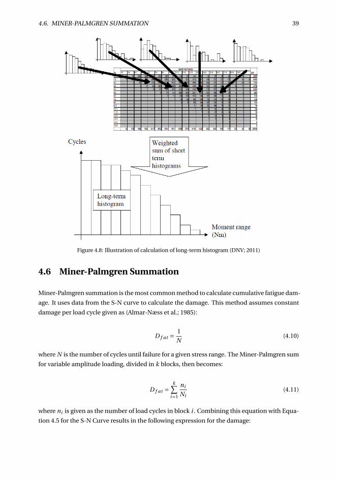
4.6. MINER-PALMGREN SUMMATION 39
Figure 4.8: Illustration of calculation of long-term histogram (DNV; 2011)
4.6 Miner-Palmgren Summation
Miner-Palmgren summation is the most common method to calculate cumulative fatigue dam-
age. It uses data from the S-N curve to calculate the damage. This method assumes constant
damage per load cycle given as (Almar-Næss et al.; 1985):
D f at =1
N(4.10)
where N is the number of cycles until failure for a given stress range. The Miner-Palmgren sum
for variable amplitude loading, divided in k blocks, then becomes:
D f at =k∑
i=1
ni
Ni(4.11)
where ni is given as the number of load cycles in block i . Combining this equation with Equa-
tion 4.5 for the S-N Curve results in the following expression for the damage:
40 CHAPTER 4. FATIGUE THEORY
D f at =1
a
k∑i=1
ni (∆Si )m (4.12)
When calculating the fatigue damage, there are different options to select the stress range for
each bin/block in the histograms. The average or maximum value of each bin can be used. An-
other option is to disregard the histogram and describe every cycle by itself, thus not gathering
them in blocks (ni = 1). In this thesis the maximum value of each bin is selected.
The fatigue design criterion is given as:
D f at ·DF F < 1 (4.13)
where DFF is the Design Fatigue Factor. The DFF is applied to reduce the probability of fa-
tigue failure, and is selected based on availability for inspection and the consequence of failure
(DNV GL; 2014). For fatigue calculations of the wellhead DFF=10 is used (DNV; 2011).
Fatigue is, as mentioned earlier, a result of cycle-by-cycle loads. Hence, the stress and strain
in a cycle, will depend on the previous cycles. This is called a stress memory effect and is not
accounted for in Miner-Palmgren summation. This effect could lead to bias and an uncertain
estimation of damage. To account for this bias a relative Miner-Palmgren sum can be applied,
and for offshore structures D < 0.5 is proposed. However, Miner-Palmgren sums are often
set to less than 1 due to the DFF, which includes an additional safety factor. This means that
Miner-Palmgren does not only measure damage, but is also a safety measure (Almar-Næss
et al.; 1985).
Chapter 5
Overall Wellhead Fatigue
Methodology
The following information is found in the Wellhead Fatigue Analysis Method (DNV; 2011).
In this chapter the wellhead fatigue analysis method developed by the Joint Industry Project is
presented. Please note that the local analysis is not performed in this thesis.
To calculate the fatigue life of a wellhead a three-step procedure is used:
1. Local response analysis
2. Global load analysis
3. Fatigue damage assessment
The analysis methodology describes how to calculate wellhead fatigue using two separate
analyses, namely one local and one global analysis. The global analysis is performed to obtain
the moment at the wellhead datum. The moments are transformed to stresses at the critical
hot spots by use of a local analysis. In addition, the local analysis establish the boundary con-
ditions at the wellhead, which are used in the global load analysis. Using the obtained stresses,
in combination with SN-curves, a Miner-Palmgren summation can be carried out to calculate
the fatigue damage. The method can be visualized in the flowchart in Figure 5.1.
The steps in the analysis procedure will be explained more thoroughly in the sections below.
41
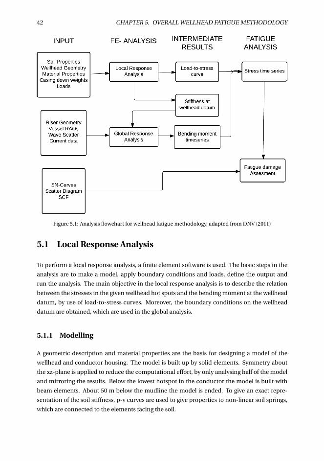
42 CHAPTER 5. OVERALL WELLHEAD FATIGUE METHODOLOGY
Figure 5.1: Analysis flowchart for wellhead fatigue methodology, adapted from DNV (2011)
5.1 Local Response Analysis
To perform a local response analysis, a finite element software is used. The basic steps in the
analysis are to make a model, apply boundary conditions and loads, define the output and
run the analysis. The main objective in the local response analysis is to describe the relation
between the stresses in the given wellhead hot spots and the bending moment at the wellhead
datum, by use of load-to-stress curves. Moreover, the boundary conditions on the wellhead
datum are obtained, which are used in the global analysis.
5.1.1 Modelling
A geometric description and material properties are the basis for designing a model of the
wellhead and conductor housing. The model is built up by solid elements. Symmetry about
the xz-plane is applied to reduce the computational effort, by only analysing half of the model
and mirroring the results. Below the lowest hotspot in the conductor the model is built with
beam elements. About 50 m below the mudline the model is ended. To give an exact repre-
sentation of the soil stiffness, p-y curves are used to give properties to non-linear soil springs,
which are connected to the elements facing the soil.
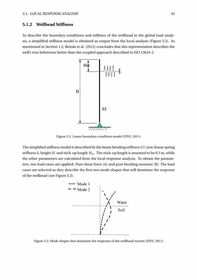
5.1. LOCAL RESPONSE ANALYSIS 43
5.1.2 Wellhead Stiffness
To describe the boundary conditions and stiffness of the wellhead in the global load analy-
sis, a simplified stiffness model is obtained as output from the local analysis (Figure 5.2). As
mentioned in Section 1.2, Reinås et al. (2012) concludes that this representation describes the
well’s true behaviour better than the coupled approach described in ISO 13624-2.
Figure 5.2: Lower boundary condition model (DNV; 2011)
The simplified stiffness model is described by the beam bending stiffness E I , non-linear spring
stiffness k, height H , and stick-up length Hst . The stick-up length is assumed to be 0.5 m, while
the other parameters are calculated from the local response analysis. To obtain the parame-
ters, two load cases are applied: Pure shear force (A) and pure bending moment (B). The load
cases are selected as they describe the first two mode shapes that will dominate the response
of the wellhead (see Figure 5.3).
Figure 5.3: Mode shapes that dominate the response of the wellhead system (DNV; 2011)
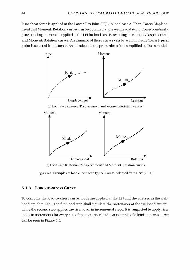
44 CHAPTER 5. OVERALL WELLHEAD FATIGUE METHODOLOGY
Pure shear force is applied at the Lower Flex Joint (LFJ), in load case A. Then, Force/Displace-
ment and Moment/Rotation curves can be obtained at the wellhead datum. Correspondingly,
pure bending moment is applied at the LFJ for load case B, resulting in Moment/Displacement
and Moment/Rotation curves. An example of these curves can be seen in Figure 5.4. A typical
point is selected from each curve to calculate the properties of the simplified stiffness model.
(a) Load case A: Force/Displacement and Moment/Rotation curves
(b) Load case B: Moment/Displacement and Moment/Rotation curves
Figure 5.4: Examples of load curves with typical Points. Adapted from DNV (2011)
5.1.3 Load-to-stress Curve
To compute the load-to-stress curve, loads are applied at the LFJ and the stresses in the well-
head are obtained. The first load step shall simulate the pretension of the wellhead system,
while the second step applies the riser load, in incremental steps. It is suggested to apply riser
loads in increments for every 5 % of the total riser load. An example of a load-to-stress curve
can be seen in Figure 5.5.
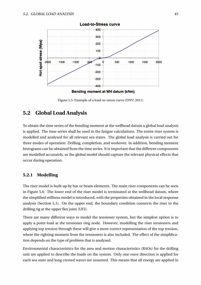
5.2. GLOBAL LOAD ANALYSIS 45
Figure 5.5: Example of a load-to-stress curve (DNV; 2011)
5.2 Global Load Analysis
To obtain the time series of the bending moment at the wellhead datum a global load analysis
is applied. The time series shall be used in the fatigue calculations. The entire riser system is
modelled and analysed for all relevant sea states. The global load analysis is carried out for
three modes of operation: Drilling, completion, and workover. In addition, bending moment
histograms can be obtained from the time series. It is important that the different components
are modelled accurately, as the global model should capture the relevant physical effects that
occur during operation.
5.2.1 Modelling
The riser model is built up by bar or beam elements. The main riser components can be seen
in Figure 5.6. The lower end of the riser model is terminated at the wellhead datum, where
the simplified stiffness model is introduced, with the properties obtained in the local response
analysis (Section 5.1). On the upper end, the boundary condition connects the riser to the
drilling rig at the upper flex joint (UFJ).
There are many different ways to model the tensioner system, but the simplest option is to
apply a point load at the tensioner ring node. However, modelling the riser tensioners and
applying top tension through these will give a more correct representation of the top tension,
where the righting moment from the tensioners is also included. The effect of the simplifica-
tion depends on the type of problem that is analysed.
Environmental characteristics for the area and motion characteristics (RAOs) for the drilling
unit are applied to describe the loads on the system. Only one wave direction is applied for
each sea state and long crested waves are assumed. This means that all energy are applied in
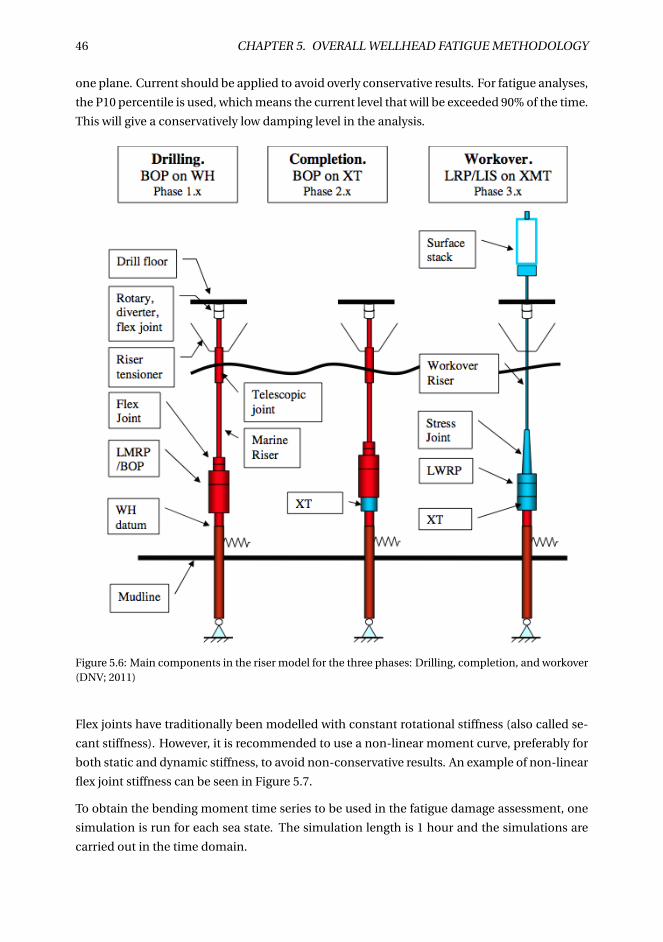
46 CHAPTER 5. OVERALL WELLHEAD FATIGUE METHODOLOGY
one plane. Current should be applied to avoid overly conservative results. For fatigue analyses,
the P10 percentile is used, which means the current level that will be exceeded 90% of the time.
This will give a conservatively low damping level in the analysis.
Figure 5.6: Main components in the riser model for the three phases: Drilling, completion, and workover(DNV; 2011)
Flex joints have traditionally been modelled with constant rotational stiffness (also called se-
cant stiffness). However, it is recommended to use a non-linear moment curve, preferably for
both static and dynamic stiffness, to avoid non-conservative results. An example of non-linear
flex joint stiffness can be seen in Figure 5.7.
To obtain the bending moment time series to be used in the fatigue damage assessment, one
simulation is run for each sea state. The simulation length is 1 hour and the simulations are
carried out in the time domain.
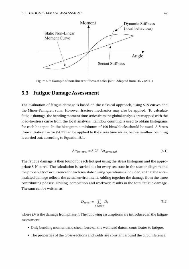
5.3. FATIGUE DAMAGE ASSESSMENT 47
Figure 5.7: Example of non-linear stiffness of a flex joint. Adapted from DNV (2011)
5.3 Fatigue Damage Assessment
The evaluation of fatigue damage is based on the classical approach, using S-N curves and
the Miner-Palmgren sum. However, fracture mechanics may also be applied. To calculate
fatigue damage, the bending moment time series from the global analysis are mapped with the
load-to-stress curve from the local analysis. Rainflow counting is used to obtain histograms
for each hot spot. In the histogram a minimum of 100 bins/blocks should be used. A Stress
Concentration Factor (SCF) can be applied to the stress time series, before rainflow counting
is carried out, according to Equation 5.1.
∆σhot spot = SC F ·∆σnomi nal (5.1)
The fatigue damage is then found for each hotspot using the stress histogram and the appro-
priate S-N curve. The calculation is carried out for every sea state in the scatter diagram and
the probability of occurrence for each sea state during operations is included, so that the accu-
mulated damage reflects the actual environment. Adding together the damage from the three
contributing phases: Drilling, completion and workover, results in the total fatigue damage.
The sum can be written as:
D tot al =∑
phasesDi (5.2)
where Di is the damage from phase i . The following assumptions are introduced in the fatigue
assessment:
• Only bending moment and shear force on the wellhead datum contributes to fatigue.
• The properties of the cross-sections and welds are constant around the circumference.

48 CHAPTER 5. OVERALL WELLHEAD FATIGUE METHODOLOGY
• Potential hysteresis effects are not taken into account. This means that the load-to-stress
curve is equal for loading and unloading.
• Hot spot stress is calculated on both the compression and tension sides, thus the load-
to-stress curve may therefore be unsymmetrical.
In the Joint Industry Project analysis methodology, which is used in this report, the contribu-
tion of vortex induced vibrations (VIV) is not included. This can be seen as a non-conservative
assumption, as some combinations of environmental conditions (current) and system prop-
erties may lead to VIV and thus cause high fatigue damage on the well.
Chapter 6
Modelling and Analysis
This chapter describes the modelling and analyses carried out in this thesis. First, the global
load analysis is presented: Input, modelling properties, and analysis set up. Second, the fa-
tigue damage calculation is described, including development of load histograms and relative
damage calculations.
6.1 Global Load Analysis
To execute the global load analyses, the computer program SIMA/RIFLEX is utilized. The over-
all global load analysis procedure is described in Section 5.2.
6.1.1 SIMA/RIFLEX
SIMA/RIFLEX is a computer tool for the global analysis of slender systems made by MAR-
INTEK. The main theory principles that it is based on are presented in Chapter 3. RIFLEX
contains five modules: INPMOD, STAMOD, DYNMOD, FREMOD, and OUTMOD (Marintek;
2014b). An overview of the structure of the program can be seen in Figure 6.1.
49
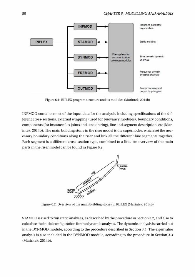
50 CHAPTER 6. MODELLING AND ANALYSIS
Figure 6.1: RIFLEX program structure and its modules (Marintek; 2014b)
INPMOD contains most of the input data for the analysis, including specifications of the dif-
ferent cross-sections, external wrapping (used for buoyancy modules), boundary conditions,
components (for instance flex joints and tension ring), line and segment description, etc (Mar-
intek; 2014b). The main building stone in the riser model is the supernodes, which set the nec-
essary boundary conditions along the riser and link all the different line segments together.
Each segment is a different cross-section type, combined to a line. An overview of the main
parts in the riser model can be found in Figure 6.2.
Figure 6.2: Overview of the main building stones in RIFLEX (Marintek; 2014b)
STAMOD is used to run static analyses, as described by the procedure in Section 3.2, and also to
calculate the initial configuration for the dynamic analysis. The dynamic analysis is carried out
in the DYNMOD module, according to the procedure described in Section 3.4. The eigenvalue
analysis is also included in the DYNMOD module, according to the procedure in Section 3.3
(Marintek; 2014b).
6.1. GLOBAL LOAD ANALYSIS 51
SIMA/RIFLEX contains a post-processing package, which is included in the OUTMOD and
PLOMOD modules. OUTMOD can be used to obtain for instance the time series and envelope
curves for forces and moments, and to carry out fatigue calculations. PLOMOD is used to plot
the results from OUTMOD (Marintek; 2014b).
6.1.2 Input Data
All modelling data are provided by Aker Solutions. The input data describe a drilling riser
model (phase 1), and this is the only phase that will be covered in the analysis. An overview of
the model can be seen in Figure 6.3. All input data can be found in Appendix A.
To investigate the effect of change in tension, five different water depths are modelled: 80m,
125m, 190m, 500m and 1000m. All models have the same stack-up, but the length of the buoy-
ant section has been changed to get the correct length for the different models.
Some important data for the models are:
• A drilling fluid density of ρd = 1500kg /m3 is applied inside the pipe.
• To simulate the movement in the telescopic joint, the inner barrel is assumed to be a
beam with low axial stiffness. For this analysis, the stiffness of the inner barrel (see Table
6.2) is divided by 100000 (Sævik; 2015). The inner barrel is also modelled so that it is
nearly mass-less.
• The model is built from the seabed and up, meaning that the bottom point is the soil
node.
• Drag- and added mass coefficients is applied to describe the hydrodynamic loads on the
structure. CDN =1, CDT =0.03, while C AN ≈1, depending on the component. Details can
be found in Appendix A.3.
• The riser model consists of two flex joints. The upper flex joint has linear stiffness, while
the lower flex joint has non-linear stiffness. The lower flex joint has a larger stiffness than
the upper flex joint. Details can be found in Appendix A.5.
• On the lower boundary the riser is connected to the wellhead. The wellhead model is
pinned, below the seabed, as seen in Figure 6.4. A spring is used to model the soil stiff-
ness. On the upper boundary the drilling riser is connected to the drilling rig, which is
modelled by a fixed boundary condition.
The length and number of elements applied for each component is given in Table 6.1.
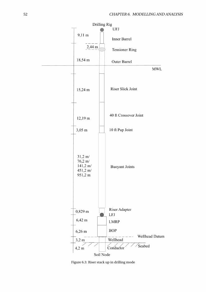
52 CHAPTER 6. MODELLING AND ANALYSIS
Figure 6.3: Riser stack up in drilling mode
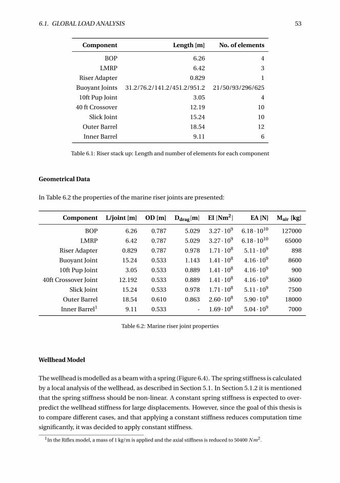
6.1. GLOBAL LOAD ANALYSIS 53
Component Length [m] No. of elements
BOP 6.26 4
LMRP 6.42 3
Riser Adapter 0.829 1
Buoyant Joints 31.2/76.2/141.2/451.2/951.2 21/50/93/296/625
10ft Pup Joint 3.05 4
40 ft Crossover 12.19 10
Slick Joint 15.24 10
Outer Barrel 18.54 12
Inner Barrel 9.11 6
Table 6.1: Riser stack up: Length and number of elements for each component
Geometrical Data
In Table 6.2 the properties of the marine riser joints are presented:
Component L/joint [m] OD [m] Ddrag[m] EI [Nm2] EA [N] Mair [kg]
BOP 6.26 0.787 5.029 3.27 ·109 6.18 ·1010 127000
LMRP 6.42 0.787 5.029 3.27 ·109 6.18 ·1010 65000
Riser Adapter 0.829 0.787 0.978 1.71 ·108 5.11 ·109 898
Buoyant Joint 15.24 0.533 1.143 1.41 ·108 4.16 ·109 8600
10ft Pup Joint 3.05 0.533 0.889 1.41 ·108 4.16 ·109 900
40ft Crossover Joint 12.192 0.533 0.889 1.41 ·108 4.16 ·109 3600
Slick Joint 15.24 0.533 0.978 1.71 ·108 5.11 ·109 7500
Outer Barrel 18.54 0.610 0.863 2.60 ·108 5.90 ·109 18000
Inner Barrel1 9.11 0.533 - 1.69 ·108 5.04 ·109 7000
Table 6.2: Marine riser joint properties
Wellhead Model
The wellhead is modelled as a beam with a spring (Figure 6.4). The spring stiffness is calculated
by a local analysis of the wellhead, as described in Section 5.1. In Section 5.1.2 it is mentioned
that the spring stiffness should be non-linear. A constant spring stiffness is expected to over-
predict the wellhead stiffness for large displacements. However, since the goal of this thesis is
to compare different cases, and that applying a constant stiffness reduces computation time
significantly, it was decided to apply constant stiffness.
1In the Riflex model, a mass of 1 kg/m is applied and the axial stiffness is reduced to 50400 N m2.
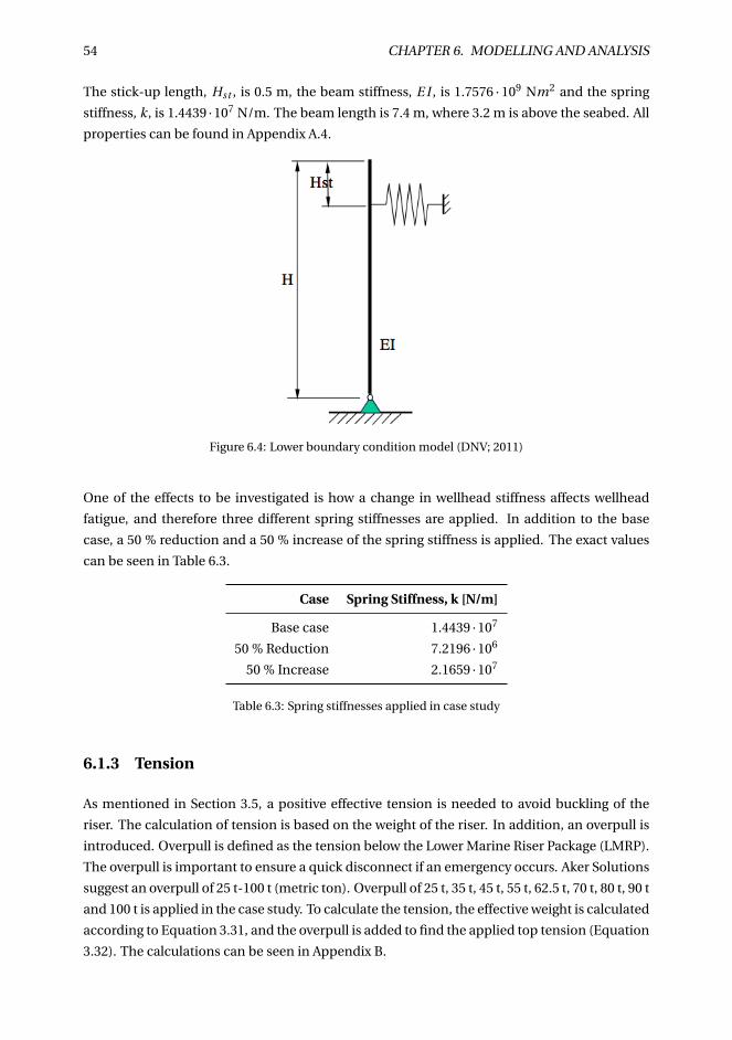
54 CHAPTER 6. MODELLING AND ANALYSIS
The stick-up length, Hst , is 0.5 m, the beam stiffness, E I , is 1.7576 · 109 Nm2 and the spring
stiffness, k, is 1.4439 ·107 N/m. The beam length is 7.4 m, where 3.2 m is above the seabed. All
properties can be found in Appendix A.4.
Figure 6.4: Lower boundary condition model (DNV; 2011)
One of the effects to be investigated is how a change in wellhead stiffness affects wellhead
fatigue, and therefore three different spring stiffnesses are applied. In addition to the base
case, a 50 % reduction and a 50 % increase of the spring stiffness is applied. The exact values
can be seen in Table 6.3.
Case Spring Stiffness, k [N/m]
Base case 1.4439 ·107
50 % Reduction 7.2196 ·106
50 % Increase 2.1659 ·107
Table 6.3: Spring stiffnesses applied in case study
6.1.3 Tension
As mentioned in Section 3.5, a positive effective tension is needed to avoid buckling of the
riser. The calculation of tension is based on the weight of the riser. In addition, an overpull is
introduced. Overpull is defined as the tension below the Lower Marine Riser Package (LMRP).
The overpull is important to ensure a quick disconnect if an emergency occurs. Aker Solutions
suggest an overpull of 25 t-100 t (metric ton). Overpull of 25 t, 35 t, 45 t, 55 t, 62.5 t, 70 t, 80 t, 90 t
and 100 t is applied in the case study. To calculate the tension, the effective weight is calculated
according to Equation 3.31, and the overpull is added to find the applied top tension (Equation
3.32). The calculations can be seen in Appendix B.
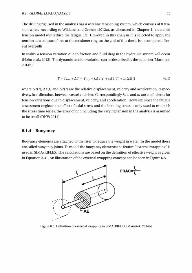
6.1. GLOBAL LOAD ANALYSIS 55
The drilling rig used in the analysis has a wireline tensioning system, which consists of 8 ten-
sion wires. According to Williams and Greene (2012a), as discussed in Chapter 1, a detailed
tension model will reduce the fatigue life. However, in this analysis it is selected to apply the
tension as a constant force at the tensioner ring, as the goal of this thesis is to compare differ-
ent overpulls.
In reality a tension variation due to friction and fluid drag in the hydraulic system will occur
(Holm et al.; 2013). The dynamic tension variation can be described by the equation (Marintek;
2014b):
T = Ttop +∆T = Ttop +k∆z(t )+ c∆z(T )+m∆z(t ) (6.1)
where ∆z(t ), ∆z(t ) and ∆z(t ) are the relative displacement, velocity and acceleration, respec-
tively, in z-direction, between vessel and riser. Correspondingly k, c, and m are coefficients for
tension variations due to displacement, velocity, and acceleration. However, since the fatigue
assessment neglects the effect of axial stress and the bending stress is only used to establish
the stress time series, the error of not including the varying tension in the analysis is assumed
to be small (DNV; 2011).
6.1.4 Buoyancy
Buoyancy elements are attached to the riser to reduce the weight in water. In the model these
are called buoyancy joints. To model the buoyancy elements the feature "external wrapping" is
used in SIMA/RIFLEX. The calculations are based on the definition of effective weight as given
in Equation 3.31. An illustration of the external wrapping concept can be seen in Figure 6.5.
Figure 6.5: Definition of external wrapping in SIMA/RIFLEX (Marintek; 2014b)
56 CHAPTER 6. MODELLING AND ANALYSIS
The length of the wrapping is equal to the length of the joint for the buoyant joints, so the
fraction is 1. The area of the external wrapping (AE) is calculated as the difference between
the hydrodynamic diameter and the outer diameter. It is assumed that the buoyancy joint
carries all of the weight, so that the external wrapping has zero mass. Hence, only the external
wrapping, AE, has to be calculated.
In the input data only the weight in air and the weight in water (open pipe) is given, so the
material density, ρmat , is calculated first from the following relation:
Msub,openpi pe = Mai r ·BF = Mai r · ρmat −ρρmat
(6.2)
where BF is the buoyancy factor, given from the material density ρmat and water density ρ.
Applying that Msub,openpi pe = 500kg and Mai r = 8600kg leads to a material density, ρmat =1088.3kg /m3. The total area of the buoyant joint is then found by:
Mai r = ρmat ·V = ρmat · A ·1 (6.3)
Resulting in a total area of 0.5185m2. From this, the cross-section outer area can be subtracted,
leading to the area of the buoyancy element, AE = 0.2955m2. A detailed calculation can be
found in Appendix C.
6.1.5 Environment
The metocean report (Statoil; 2010) for the field is used to specify the environmental condition
for the model. In accordance with the practice for fatigue, the P10 percentile is used when
applying current (i.e a current level that will be exceeded 90 % of the time (DNV; 2011)), with
vc = 0.05m/s. Uniform current along the riser is assumed. This will result in a conservatively
low damping level (DNV; 2011).
To obtain the most accurate results, irregular waves are used. They are generated from the
JONSWAP spectrum, as described in Section 3.7. As the waves are long crested, a unidirec-
tional JONSWAP spectrum is applied. A significant wave height of 3.5 m and peak periods in
the interval between 4.5 - 20.5 sec is applied in the global analysis, according to the problem
text. The scatter diagram is given in Table 6.4.
In reality, every sea state has its own main direction, but to simplify the analysis, only one wave
heading is used. The drilling riser itself can be assumed to be axis-symmetric, so the main dif-
ference in loading comes from the motions of the drilling rig, which will vary with the wave
direction. For this analysis, only a 0◦ heading is used (head sea), thus surge will be the dom-
inating motion. The transfer function for surge can be seen in Figure 6.6. As surge motion
will lead to displacement of the riser, this will result in a bending moment on the wellhead.
Applying only one heading in the analyses is expected to be a conservative assumption, since
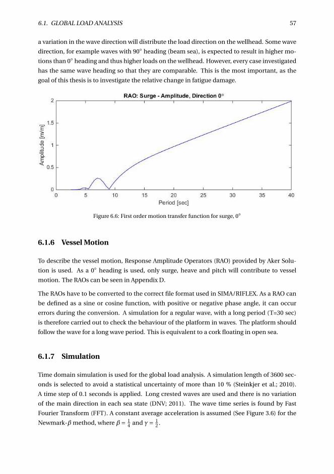
6.1. GLOBAL LOAD ANALYSIS 57
a variation in the wave direction will distribute the load direction on the wellhead. Some wave
direction, for example waves with 90◦ heading (beam sea), is expected to result in higher mo-
tions than 0◦ heading and thus higher loads on the wellhead. However, every case investigated
has the same wave heading so that they are comparable. This is the most important, as the
goal of this thesis is to investigate the relative change in fatigue damage.
Figure 6.6: First order motion transfer function for surge, 0◦
6.1.6 Vessel Motion
To describe the vessel motion, Response Amplitude Operators (RAO) provided by Aker Solu-
tion is used. As a 0◦ heading is used, only surge, heave and pitch will contribute to vessel
motion. The RAOs can be seen in Appendix D.
The RAOs have to be converted to the correct file format used in SIMA/RIFLEX. As a RAO can
be defined as a sine or cosine function, with positive or negative phase angle, it can occur
errors during the conversion. A simulation for a regular wave, with a long period (T=30 sec)
is therefore carried out to check the behaviour of the platform in waves. The platform should
follow the wave for a long wave period. This is equivalent to a cork floating in open sea.
6.1.7 Simulation
Time domain simulation is used for the global load analysis. A simulation length of 3600 sec-
onds is selected to avoid a statistical uncertainty of more than 10 % (Steinkjer et al.; 2010).
A time step of 0.1 seconds is applied. Long crested waves are used and there is no variation
of the main direction in each sea state (DNV; 2011). The wave time series is found by Fast
Fourier Transform (FFT). A constant average acceleration is assumed (See Figure 3.6) for the
Newmark-β method, where β= 14 and γ= 1
2 .
58 CHAPTER 6. MODELLING AND ANALYSIS
The damping parameters are calculated according to Section 3.1.3. According to Langen and
Sigbjörnsson (1979), it can be assumed for risers that α1 = 0. If a typical damping level of 3% is
assumed, then Equation 3.11 can be simplified and solved for α2:
0.03 = 1
2α2ω (6.4)
α2 = 0.06T
2π(6.5)
To simplify the analysis, one single period is selected. To be conservative, a small α2 is desir-
able. Hence, a low period is selected. For a period of 1 sec, α2 = 0.009.
6.2 Fatigue Damage Assessment
From the global load analysis, the time series of the bending moment are obtained and fatigue
calculations, as described in Chapter 4 are carried out.
The bending moment time series obtained in the global load analysis are used to develop
bending moment histograms, applying the rainflow counting procedure. As mentioned in Sec-
tion 4.4 there are many different ways to account for half cycles, and in this thesis it is selected
to count them as a half of a full cycle. In MATLAB histograms are computed by utilizing the
WAFO package (Brodtkorb et al.; 2000). Both short- and long-term histograms are obtained, as
described by the procedure in Section 4.5. The histograms are divided in bins of 5000 Nm. The
scatter weight applied to calculate the long term/weighted histograms is given in Table 6.4.
The scatter diagram is given for significant wave height (Hs ) and spectral peak period (Tp ), for
a period of 100 years and is calculated from the long-term wave statistics (Statoil; 2010).
In addition, a relative fatigue damage calculation is carried out, applying Miner-Palmgren
summation. The damage is calculated for 1 hour. The reason that the term relative fatigue
damage is used in this thesis, is that the conversion from loads to stresses is not carried out.
Instead, it is assumed that the stress is linearly dependent on the bending moment and thus
the fatigue damage calculated with the use of bending moment will be proportional to the
actual fatigue damage. The results in terms of numerical values can therefore not be used to
define the actual fatigue life, but only to do a relative comparison between the different cases.
Due to these factors, the Design Fatigue Factor (DFF) is not taken into account. The S-N curve
applied is F1, which is for a single-sided weld in a seawater environment with cathodic pro-
tection. The SN-curve is chosen according to DNVGL-RP-0005 (DNV GL; 2014). According to
the problem text it is assumed that the fatigue damage will be in the high cycle range-regime
(N < 107) and thus m=5 is applied for the SN-curve. As a result the SN-curve is a straight line
and not bi-linear.
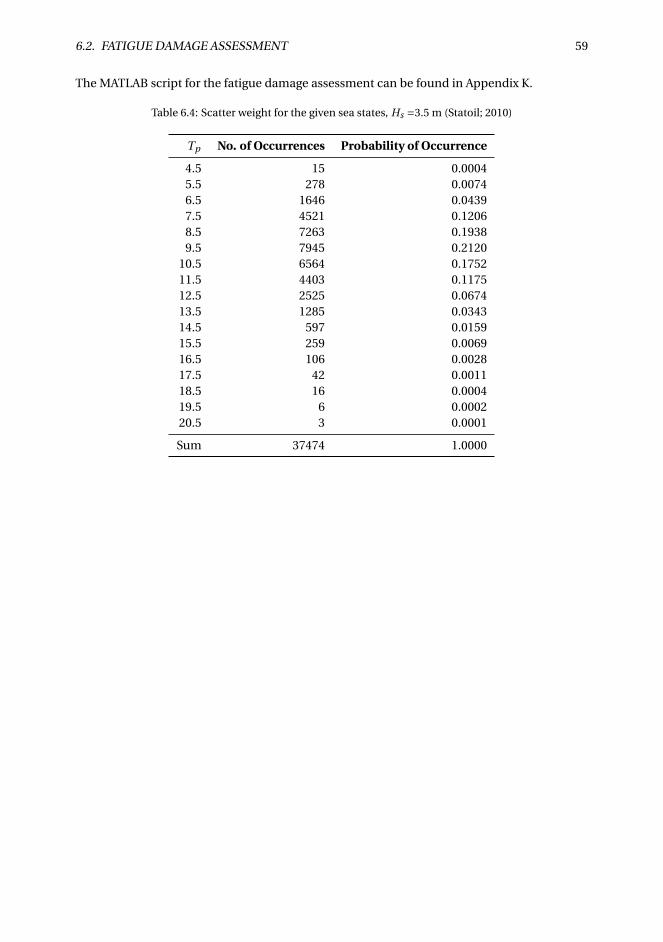
6.2. FATIGUE DAMAGE ASSESSMENT 59
The MATLAB script for the fatigue damage assessment can be found in Appendix K.
Table 6.4: Scatter weight for the given sea states, Hs =3.5 m (Statoil; 2010)
Tp No. of Occurrences Probability of Occurrence
4.5 15 0.00045.5 278 0.00746.5 1646 0.04397.5 4521 0.12068.5 7263 0.19389.5 7945 0.2120
10.5 6564 0.175211.5 4403 0.117512.5 2525 0.067413.5 1285 0.034314.5 597 0.015915.5 259 0.006916.5 106 0.002817.5 42 0.001118.5 16 0.000419.5 6 0.000220.5 3 0.0001
Sum 37474 1.0000

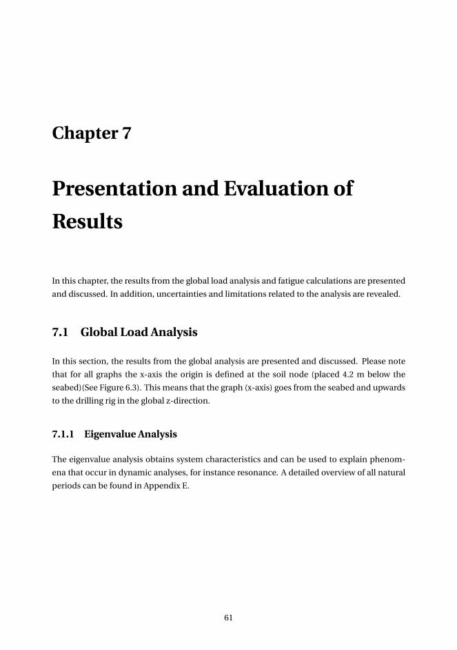
Chapter 7
Presentation and Evaluation of
Results
In this chapter, the results from the global load analysis and fatigue calculations are presented
and discussed. In addition, uncertainties and limitations related to the analysis are revealed.
7.1 Global Load Analysis
In this section, the results from the global analysis are presented and discussed. Please note
that for all graphs the x-axis the origin is defined at the soil node (placed 4.2 m below the
seabed)(See Figure 6.3). This means that the graph (x-axis) goes from the seabed and upwards
to the drilling rig in the global z-direction.
7.1.1 Eigenvalue Analysis
The eigenvalue analysis obtains system characteristics and can be used to explain phenom-
ena that occur in dynamic analyses, for instance resonance. A detailed overview of all natural
periods can be found in Appendix E.
61
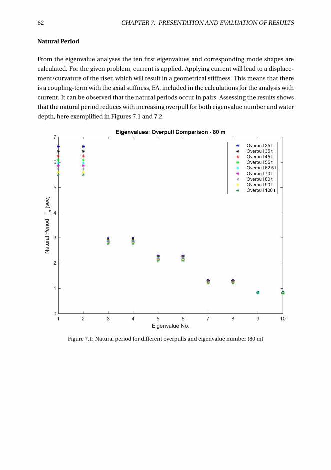
62 CHAPTER 7. PRESENTATION AND EVALUATION OF RESULTS
Natural Period
From the eigenvalue analyses the ten first eigenvalues and corresponding mode shapes are
calculated. For the given problem, current is applied. Applying current will lead to a displace-
ment/curvature of the riser, which will result in a geometrical stiffness. This means that there
is a coupling-term with the axial stiffness, EA, included in the calculations for the analysis with
current. It can be observed that the natural periods occur in pairs. Assessing the results shows
that the natural period reduces with increasing overpull for both eigenvalue number and water
depth, here exemplified in Figures 7.1 and 7.2.
Figure 7.1: Natural period for different overpulls and eigenvalue number (80 m)
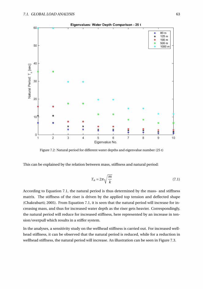
7.1. GLOBAL LOAD ANALYSIS 63
Figure 7.2: Natural period for different water depths and eigenvalue number (25 t)
This can be explained by the relation between mass, stiffness and natural period:
Tn = 2π
√m
k(7.1)
According to Equation 7.1, the natural period is thus determined by the mass- and stiffness
matrix. The stiffness of the riser is driven by the applied top tension and deflected shape
(Chakrabarti; 2005). From Equation 7.1, it is seen that the natural period will increase for in-
creasing mass, and thus for increased water depth as the riser gets heavier. Correspondingly,
the natural period will reduce for increased stiffness, here represented by an increase in ten-
sion/overpull which results in a stiffer system.
In the analyses, a sensitivity study on the wellhead stiffness is carried out. For increased well-
head stiffness, it can be observed that the natural period is reduced, while for a reduction in
wellhead stiffness, the natural period will increase. An illustration can be seen in Figure 7.3.
64 CHAPTER 7. PRESENTATION AND EVALUATION OF RESULTS
Figure 7.3: Natural period for different wellhead stiffness (25 t, 80 m)
According to Equation 7.1 it is observed that an increase in the overall stiffness, k, due to the in-
creased wellhead stiffness will result in a reduced natural period. Thus, the results correspond
with the proposed theory.
From Figure 7.3, it can be observed that the change in natural period, especially for the most
dominating eigenvalues, 1 and 2, is seen to be relatively small for the change in wellhead stiff-
ness. Hence, it is possible that the change in wellhead stiffness has small effect on the total
stiffness and thus a small effect on the system’s overall response.
Mode Shape
Each eigenvalue have a corresponding mode shape. For the given problem, the eigenvalues
occur in pairs, as seen in Figure 7.1-7.3 and in Appendix E. Thus, the mode shapes will also oc-
cur in pairs. The only difference between the mode shapes in each pair is the direction where
the largest displacement occurs (changing between X and Y-displacement). X-direction is the
direction of the incoming waves- and current, while Y-direction is the transverse direction.
Since the mode shapes occur in pairs, only one mode shape is displayed for each pair. It is ex-
pected that the mode shapes will be similar to the fundamental mode shapes, which according
to Larsen (2012) are given as:
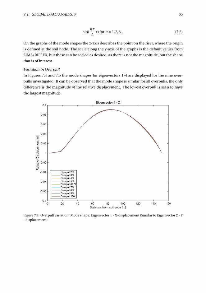
7.1. GLOBAL LOAD ANALYSIS 65
sin(nπ
Lx) for n = 1,2,3... (7.2)
On the graphs of the mode shapes the x-axis describes the point on the riser, where the origin
is defined at the soil node. The scale along the y-axis of the graphs is the default values from
SIMA/RIFLEX, but these can be scaled as desired, as there is not the magnitude, but the shape
that is of interest.
Variation in Overpull
In Figures 7.4 and 7.5 the mode shapes for eigenvectors 1-4 are displayed for the nine over-
pulls investigated. It can be observed that the mode shape is similar for all overpulls, the only
difference is the magnitude of the relative displacement. The lowest overpull is seen to have
the largest magnitude.
Figure 7.4: Overpull variation: Mode shape: Eigenvector 1 - X-displacement (Similar to Eigenvector 2 - Y- displacement)
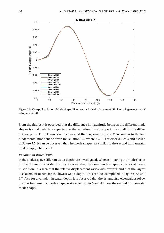
66 CHAPTER 7. PRESENTATION AND EVALUATION OF RESULTS
Figure 7.5: Overpull variation: Mode shape: Eigenvector 3 - X-displacement (Similar to Eigenvector 4 - Y- displacement)
From the figures it is observed that the difference in magnitude between the different mode
shapes is small, which is expected, as the variation in natural period is small for the differ-
ent overpulls. From Figure 7.4 it is observed that eigenvalues 1 and 2 are similar to the first
fundamental mode shape given by Equation 7.2, where n = 1. For eigenvalues 3 and 4 given
in Figure 7.5, it can be observed that the mode shapes are similar to the second fundamental
mode shape, where n = 2.
Variation in Water Depth
In the analyses, five different water depths are investigated. When comparing the mode shapes
for the different water depths it is observed that the same mode shapes occur for all cases.
In addition, it is seen that the relative displacement varies with overpull and that the largest
displacement occurs for the lowest water depth. This can be exemplified in Figures 7.6 and
7.7. Also for a variation in water depth, it is observed that the 1st and 2nd eigenvalues follow
the first fundamental mode shape, while eigenvalues 3 and 4 follow the second fundamental
mode shape.
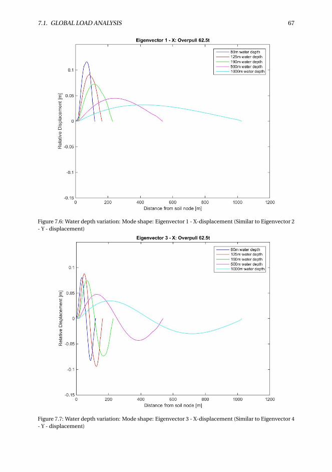
7.1. GLOBAL LOAD ANALYSIS 67
Figure 7.6: Water depth variation: Mode shape: Eigenvector 1 - X-displacement (Similar to Eigenvector 2- Y - displacement)
Figure 7.7: Water depth variation: Mode shape: Eigenvector 3 - X-displacement (Similar to Eigenvector 4- Y - displacement)
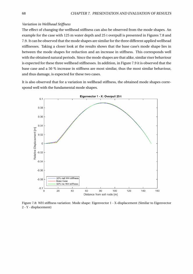
68 CHAPTER 7. PRESENTATION AND EVALUATION OF RESULTS
Variation in Wellhead Stiffness
The effect of changing the wellhead stiffness can also be observed from the mode shapes. An
example for the case with 125 m water depth and 25 t overpull is presented in Figures 7.8 and
7.9. It can be observed that the mode shapes are similar for the three different applied wellhead
stiffnesses. Taking a closer look at the results shows that the base case’s mode shape lies in
between the mode shapes for reduction and an increase in stiffness. This corresponds well
with the obtained natural periods. Since the mode shapes are that alike, similar riser behaviour
is expected for these three wellhead stiffnesses. In addition, in Figure 7.9 it is observed that the
base case and a 50 % increase in stiffness are most similar, thus the most similar behaviour,
and thus damage, is expected for these two cases.
It is also observed that for a variation in wellhead stiffness, the obtained mode shapes corre-
spond well with the fundamental mode shapes.
Figure 7.8: WH stiffness variation: Mode shape: Eigenvector 1 - X-displacement (Similar to Eigenvector2 - Y - displacement)
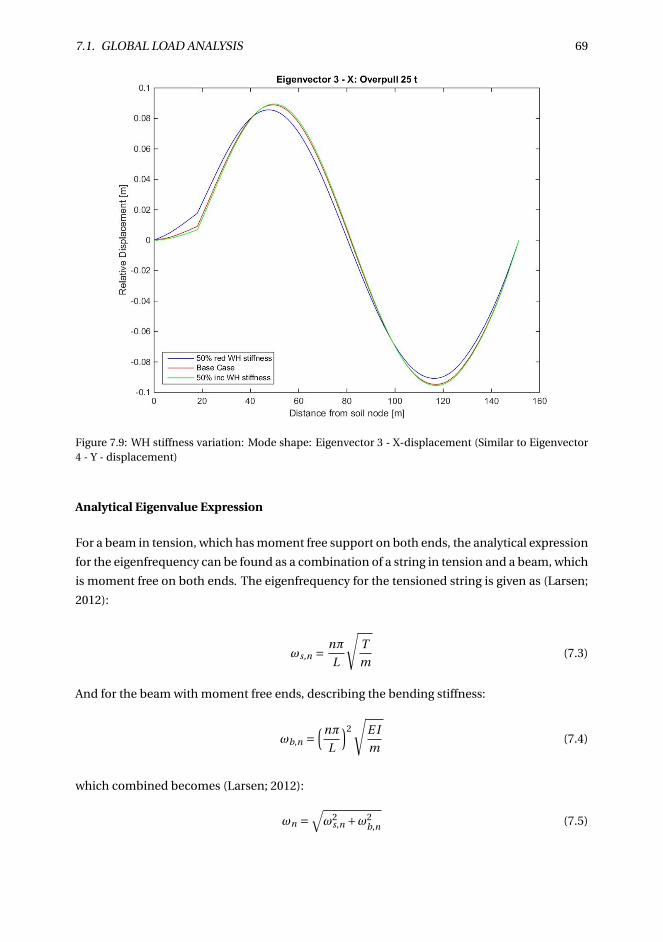
7.1. GLOBAL LOAD ANALYSIS 69
Figure 7.9: WH stiffness variation: Mode shape: Eigenvector 3 - X-displacement (Similar to Eigenvector4 - Y - displacement)
Analytical Eigenvalue Expression
For a beam in tension, which has moment free support on both ends, the analytical expression
for the eigenfrequency can be found as a combination of a string in tension and a beam, which
is moment free on both ends. The eigenfrequency for the tensioned string is given as (Larsen;
2012):
ωs,n = nπ
L
√T
m(7.3)
And for the beam with moment free ends, describing the bending stiffness:
ωb,n =(nπ
L
)2√
E I
m(7.4)
which combined becomes (Larsen; 2012):
ωn =√ω2
s,n +ω2b,n (7.5)
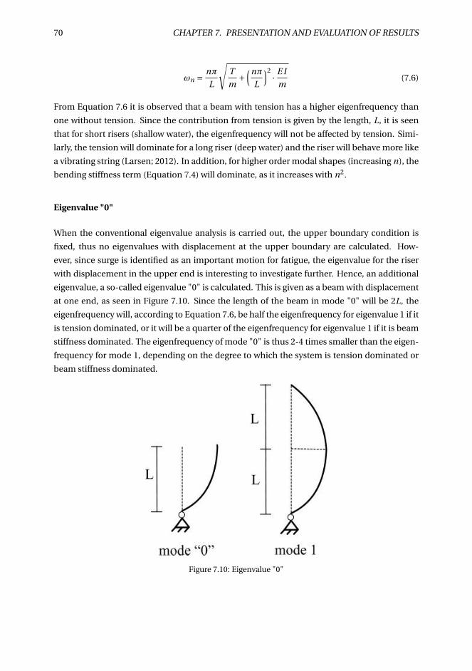
70 CHAPTER 7. PRESENTATION AND EVALUATION OF RESULTS
ωn = nπ
L
√T
m+
(nπ
L
)2· E I
m(7.6)
From Equation 7.6 it is observed that a beam with tension has a higher eigenfrequency than
one without tension. Since the contribution from tension is given by the length, L, it is seen
that for short risers (shallow water), the eigenfrequency will not be affected by tension. Simi-
larly, the tension will dominate for a long riser (deep water) and the riser will behave more like
a vibrating string (Larsen; 2012). In addition, for higher order modal shapes (increasing n), the
bending stiffness term (Equation 7.4) will dominate, as it increases with n2.
Eigenvalue "0"
When the conventional eigenvalue analysis is carried out, the upper boundary condition is
fixed, thus no eigenvalues with displacement at the upper boundary are calculated. How-
ever, since surge is identified as an important motion for fatigue, the eigenvalue for the riser
with displacement in the upper end is interesting to investigate further. Hence, an additional
eigenvalue, a so-called eigenvalue "0" is calculated. This is given as a beam with displacement
at one end, as seen in Figure 7.10. Since the length of the beam in mode "0" will be 2L, the
eigenfrequency will, according to Equation 7.6, be half the eigenfrequency for eigenvalue 1 if it
is tension dominated, or it will be a quarter of the eigenfrequency for eigenvalue 1 if it is beam
stiffness dominated. The eigenfrequency of mode "0" is thus 2-4 times smaller than the eigen-
frequency for mode 1, depending on the degree to which the system is tension dominated or
beam stiffness dominated.
Figure 7.10: Eigenvalue "0"
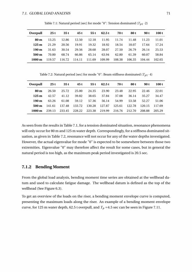
7.1. GLOBAL LOAD ANALYSIS 71
Table 7.1: Natural period [sec] for mode "0": Tension dominated (Tp1 ·2)
Overpull 25 t 35 t 45 t 55 t 62.5 t 70 t 80 t 90 t 100 t
80 m 13.25 12.86 12.50 12.18 11.95 11.74 11.48 11.23 11.01
125 m 21.29 20.56 19.91 19.32 18.92 18.54 18.07 17.64 17.24
190 m 31.63 30.54 29.56 28.68 28.07 27.50 26.79 26.14 25.53
500 m 70.80 68.74 66.86 65.14 63.94 62.80 61.39 60.07 58.84
1000 m 119.57 116.72 114.11 111.69 109.99 108.38 106.35 104.44 102.65
Table 7.2: Natural period [sec] for mode "0": Beam stiffness dominated (Tp1 ·4)
Overpull 25 t 35 t 45 t 55 t 62.5 t 70 t 80 t 90 t 100 t
80 m 26.50 25.72 25.00 24.35 23.90 23.48 22.95 22.46 22.01
125 m 42.57 41.12 39.82 38.65 37.84 37.08 36.14 35.27 34.47
190 m 63.26 61.08 59.12 57.36 56.14 54.99 53.58 52.27 51.06
500 m 141.61 137.48 133.72 130.28 127.87 125.61 122.78 120.15 117.69
1000 m 239.13 233.45 228.22 223.38 219.99 216.76 212.70 208.88 205.29
As seen from the results in Table 7.1, for a tension dominated situation, resonance phenomena
will only occur for 80 m and 125 m water depth. Correspondingly, for a stiffness dominated sit-
uation, as given in Table 7.2, resonance will not occur for any of the water depths investigated.
However, the actual eigenvalue for mode "0" is expected to be somewhere between those two
extremities. Eigenvalue "0" may therefore affect the result for some cases, but in general the
natural period is too high, as the maximum peak period investigated is 20.5 sec.
7.1.2 Bending Moment
From the global load analysis, bending moment time series are obtained at the wellhead da-
tum and used to calculate fatigue damage. The wellhead datum is defined as the top of the
wellhead (See Figure 6.3).
To get an overview of the loads on the riser, a bending moment envelope curve is computed,
presenting the maximum loads along the riser. An example of a bending moment envelope
curve, for 125 m water depth, 62.5 t overpull, and Tp =4.5 sec can be seen in Figure 7.11.
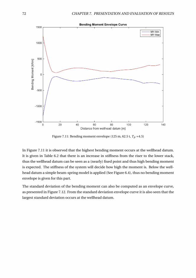
72 CHAPTER 7. PRESENTATION AND EVALUATION OF RESULTS
Figure 7.11: Bending moment envelope (125 m, 62.5 t, Tp =4.5)
In Figure 7.11 it is observed that the highest bending moment occurs at the wellhead datum.
It is given in Table 6.2 that there is an increase in stiffness from the riser to the lower stack,
thus the wellhead datum can be seen as a (nearly) fixed point and thus high bending moment
is expected. The stiffness of the system will decide how high the moment is. Below the well-
head datum a simple beam-spring model is applied (See Figure 6.4), thus no bending moment
envelope is given for this part.
The standard deviation of the bending moment can also be computed as an envelope curve,
as presented in Figure 7.12. From the standard deviation envelope curve it is also seen that the
largest standard deviation occurs at the wellhead datum.
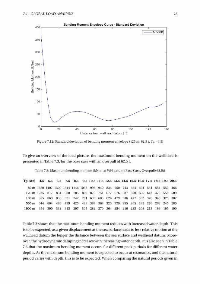
7.1. GLOBAL LOAD ANALYSIS 73
Figure 7.12: Standard deviation of bending moment envelope (125 m, 62.5 t, Tp =4.5)
To give an overview of the load picture, the maximum bending moment on the wellhead is
presented in Table 7.3, for the base case with an overpull of 62.5 t.
Table 7.3: Maximum bending moment [kNm] at WH datum (Base Case, Overpull=62.5t)
Tp [sec] 4.5 5.5 6.5 7.5 8.5 9.5 10.5 11.5 12.5 13.5 14.5 15.5 16.5 17.5 18.5 19.5 20.5
80 m 1380 1407 1300 1344 1146 1038 998 940 834 750 743 664 594 554 554 550 466
125 m 1235 817 834 988 785 809 870 751 677 676 687 670 605 613 470 558 509
190 m 985 869 836 821 742 701 639 603 626 479 536 477 392 370 348 325 307
500 m 644 604 486 439 425 428 389 364 325 329 295 265 285 276 268 245 280
1000 m 454 390 332 313 297 305 282 270 264 254 216 223 208 213 196 195 190
Table 7.3 shows that the maximum bending moment reduces with increased water depth. This
is to be expected, as a given displacement at the sea surface leads to less relative motion at the
wellhead datum the longer the distance between the sea surface and wellhead datum. More-
over, the hydrodynamic damping increases with increasing water depth. It is also seen in Table
7.3 that the maximum bending moment occurs for different peak periods for different water
depths. As the maximum bending moment is expected to occur at resonance, and the natural
period varies with depth, this is to be expected. When comparing the natural periods given in
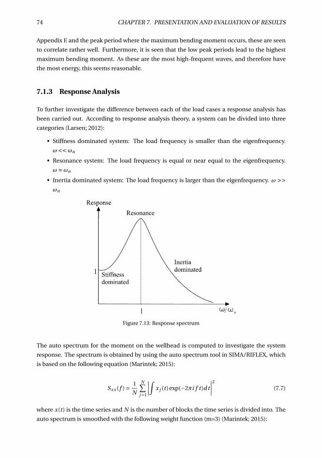
74 CHAPTER 7. PRESENTATION AND EVALUATION OF RESULTS
Appendix E and the peak period where the maximum bending moment occurs, these are seen
to correlate rather well. Furthermore, it is seen that the low peak periods lead to the highest
maximum bending moment. As these are the most high-frequent waves, and therefore have
the most energy, this seems reasonable.
7.1.3 Response Analysis
To further investigate the difference between each of the load cases a response analysis has
been carried out. According to response analysis theory, a system can be divided into three
categories (Larsen; 2012):
• Stiffness dominated system: The load frequency is smaller than the eigenfrequency.
ω<<ωn
• Resonance system: The load frequency is equal or near equal to the eigenfrequency.
ω≈ωn
• Inertia dominated system: The load frequency is larger than the eigenfrequency. ω >>ωn
Figure 7.13: Response spectrum
The auto spectrum for the moment on the wellhead is computed to investigate the system
response. The spectrum is obtained by using the auto spectrum tool in SIMA/RIFLEX, which
is based on the following equation (Marintek; 2015):
Sxx ( f ) = 1
N
N∑j=1
∣∣∣∣∫ x j (t )exp(−2πi f t )d t
∣∣∣∣2
(7.7)
where x(t ) is the time series and N is the number of blocks the time series is divided into. The
auto spectrum is smoothed with the following weight function (m=3) (Marintek; 2015):
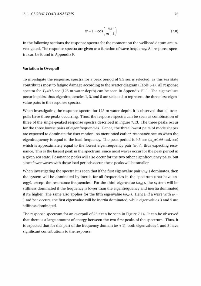
7.1. GLOBAL LOAD ANALYSIS 75
w = 1−cos
(πk
m +1
)(7.8)
In the following sections the response spectra for the moment on the wellhead datum are in-
vestigated. The response spectra are given as a function of wave frequency. All response spec-
tra can be found in Appendix F.
Variation in Overpull
To investigate the response, spectra for a peak period of 9.5 sec is selected, as this sea state
contributes most to fatigue damage according to the scatter diagram (Table 6.4). All response
spectra for Tp =9.5 sec (125 m water depth) can be seen in Appendix F.1.1. The eigenvalues
occur in pairs, thus eigenfrequencies 1, 3, and 5 are selected to represent the three first eigen-
value pairs in the response spectra.
When investigating the response spectra for 125 m water depth, it is observed that all over-
pulls have three peaks occurring. Thus, the response spectra can be seen as combination of
three of the single-peaked response spectra described in Figure 7.13. The three peaks occur
for the three lowest pairs of eigenfrequencies. Hence, the three lowest pairs of mode shapes
are expected to dominate the riser motion. As mentioned earlier, resonance occurs when the
eigenfrequency is equal to the load frequency. The peak period is 9.5 sec (ωp =0.66 rad/sec)
which is approximately equal to the lowest eigenfrequency pair (ωn1), thus expecting reso-
nance. This is the largest peak in the spectrum, since most waves occur for the peak period in
a given sea state. Resonance peaks will also occur for the two other eigenfrequency pairs, but
since fewer waves with those load periods occur, these peaks will be smaller.
When investigating the spectra it is seen that if the first eigenvalue pair (ωn1) dominates, then
the system will be dominated by inertia for all frequencies in the spectrum (that have en-
ergy), except the resonance frequencies. For the third eigenvalue (ωn3), the system will be
stiffness dominated if the frequency is lower than the eigenfrequency and inertia dominated
if it’s higher. The same also applies for the fifth eigenvalue (ωn5). Hence, if a wave with ω =1 rad/sec occurs, the first eigenvalue will be inertia dominated, while eigenvalues 3 and 5 are
stiffness dominated.
The response spectrum for an overpull of 25 t can be seen in Figure 7.14. It can be observed
that there is a large amount of energy between the two first peaks of the spectrum. Thus, it
is expected that for this part of the frequency domain (ω ≈ 1), both eigenvalues 1 and 3 have
significant contributions to the response.
76 CHAPTER 7. PRESENTATION AND EVALUATION OF RESULTS
Figure 7.14: Wellhead response: 25 t overpull (Tp =9.5 sec, 125 m)
When increasing the overpull, it can be observed that energy between the peaks in the spec-
trum reduces. For an overpull of 100 t (Figure 7.15), the energy between the first and second
peak is seen as drastically reduced compared to 25 t overpull. Hence, more of the energy is
stored in the peaks, increasing their maxima. The first peak (ωn1) more than doubles in mag-
nitude when the overpull is increased from 25 t to 100 t. When investigating the response
spectra for 100 t, it can also be observed that the third peak (ωn5) has a higher peak than the
second peak (ωn3). Thus, it is expected that the riser is more affected by eigenvalue 3 than
eigenvalue 2 for an overpull of 100 t.
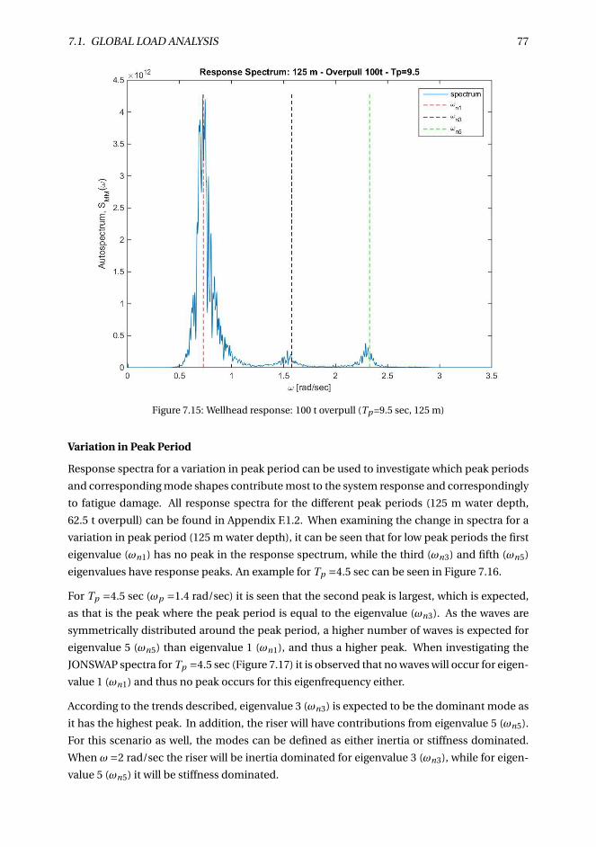
7.1. GLOBAL LOAD ANALYSIS 77
Figure 7.15: Wellhead response: 100 t overpull (Tp =9.5 sec, 125 m)
Variation in Peak Period
Response spectra for a variation in peak period can be used to investigate which peak periods
and corresponding mode shapes contribute most to the system response and correspondingly
to fatigue damage. All response spectra for the different peak periods (125 m water depth,
62.5 t overpull) can be found in Appendix F.1.2. When examining the change in spectra for a
variation in peak period (125 m water depth), it can be seen that for low peak periods the first
eigenvalue (ωn1) has no peak in the response spectrum, while the third (ωn3) and fifth (ωn5)
eigenvalues have response peaks. An example for Tp =4.5 sec can be seen in Figure 7.16.
For Tp =4.5 sec (ωp =1.4 rad/sec) it is seen that the second peak is largest, which is expected,
as that is the peak where the peak period is equal to the eigenvalue (ωn3). As the waves are
symmetrically distributed around the peak period, a higher number of waves is expected for
eigenvalue 5 (ωn5) than eigenvalue 1 (ωn1), and thus a higher peak. When investigating the
JONSWAP spectra for Tp =4.5 sec (Figure 7.17) it is observed that no waves will occur for eigen-
value 1 (ωn1) and thus no peak occurs for this eigenfrequency either.
According to the trends described, eigenvalue 3 (ωn3) is expected to be the dominant mode as
it has the highest peak. In addition, the riser will have contributions from eigenvalue 5 (ωn5).
For this scenario as well, the modes can be defined as either inertia or stiffness dominated.
When ω=2 rad/sec the riser will be inertia dominated for eigenvalue 3 (ωn3), while for eigen-
value 5 (ωn5) it will be stiffness dominated.
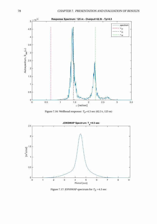
78 CHAPTER 7. PRESENTATION AND EVALUATION OF RESULTS
Figure 7.16: Wellhead response: Tp =4.5 sec (62.5 t, 125 m)
Figure 7.17: JONSWAP spectrum for Tp =4.5 sec
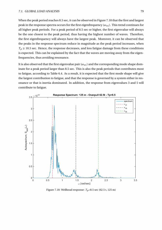
7.1. GLOBAL LOAD ANALYSIS 79
When the peak period reaches 8.5 sec, it can be observed in Figure 7.18 that the first and largest
peak in the response spectra occurs for the first eigenfrequency (ωn1). This trend continues for
all higher peak periods. For a peak period of 8.5 sec or higher, the first eigenvalue will always
be the one closest to the peak period, thus having the highest number of waves. Therefore,
the first eigenfrequency will always have the largest peak. Moreover, it can be observed that
the peaks in the response spectrum reduce in magnitude as the peak period increases, when
Tp ≥ 10.5 sec. Hence, the response decreases, and less fatigue damage from these conditions
is expected. This can be explained by the fact that the waves are moving away from the eigen-
frequencies, thus avoiding resonance.
It is also observed that the first eigenvalue pair (ωn1) and the corresponding mode shape dom-
inate for a peak period larger than 8.5 sec. This is also the peak periods that contributes most
to fatigue, according to Table 6.4. As a result, it is expected that the first mode shape will give
the largest contribution to fatigue, and that the response is governed by a system either in res-
onance or that is inertia dominated. In addition, the response from eigenvalues 3 and 5 will
contribute to fatigue.
Figure 7.18: Wellhead response: Tp =8.5 sec (62.5 t, 125 m)
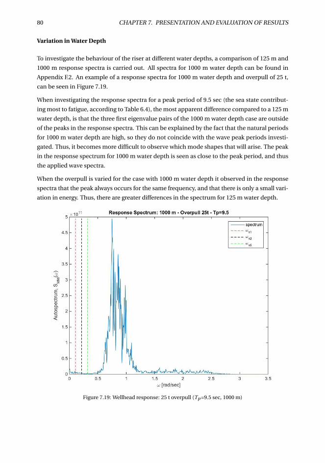
80 CHAPTER 7. PRESENTATION AND EVALUATION OF RESULTS
Variation in Water Depth
To investigate the behaviour of the riser at different water depths, a comparison of 125 m and
1000 m response spectra is carried out. All spectra for 1000 m water depth can be found in
Appendix F.2. An example of a response spectra for 1000 m water depth and overpull of 25 t,
can be seen in Figure 7.19.
When investigating the response spectra for a peak period of 9.5 sec (the sea state contribut-
ing most to fatigue, according to Table 6.4), the most apparent difference compared to a 125 m
water depth, is that the three first eigenvalue pairs of the 1000 m water depth case are outside
of the peaks in the response spectra. This can be explained by the fact that the natural periods
for 1000 m water depth are high, so they do not coincide with the wave peak periods investi-
gated. Thus, it becomes more difficult to observe which mode shapes that will arise. The peak
in the response spectrum for 1000 m water depth is seen as close to the peak period, and thus
the applied wave spectra.
When the overpull is varied for the case with 1000 m water depth it observed in the response
spectra that the peak always occurs for the same frequency, and that there is only a small vari-
ation in energy. Thus, there are greater differences in the spectrum for 125 m water depth.
Figure 7.19: Wellhead response: 25 t overpull (Tp =9.5 sec, 1000 m)
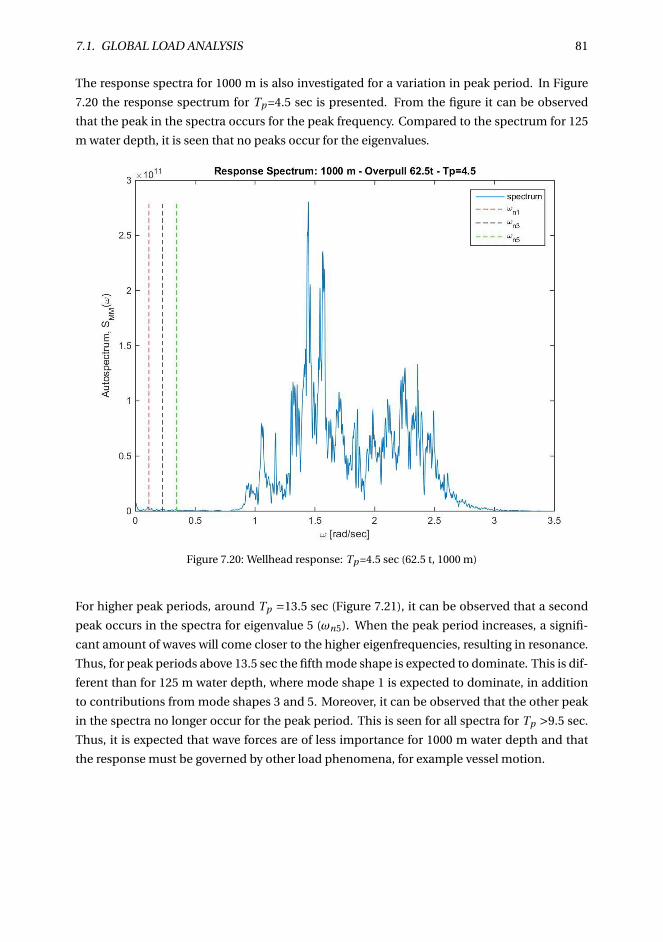
7.1. GLOBAL LOAD ANALYSIS 81
The response spectra for 1000 m is also investigated for a variation in peak period. In Figure
7.20 the response spectrum for Tp =4.5 sec is presented. From the figure it can be observed
that the peak in the spectra occurs for the peak frequency. Compared to the spectrum for 125
m water depth, it is seen that no peaks occur for the eigenvalues.
Figure 7.20: Wellhead response: Tp =4.5 sec (62.5 t, 1000 m)
For higher peak periods, around Tp =13.5 sec (Figure 7.21), it can be observed that a second
peak occurs in the spectra for eigenvalue 5 (ωn5). When the peak period increases, a signifi-
cant amount of waves will come closer to the higher eigenfrequencies, resulting in resonance.
Thus, for peak periods above 13.5 sec the fifth mode shape is expected to dominate. This is dif-
ferent than for 125 m water depth, where mode shape 1 is expected to dominate, in addition
to contributions from mode shapes 3 and 5. Moreover, it can be observed that the other peak
in the spectra no longer occur for the peak period. This is seen for all spectra for Tp >9.5 sec.
Thus, it is expected that wave forces are of less importance for 1000 m water depth and that
the response must be governed by other load phenomena, for example vessel motion.
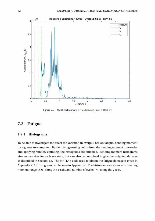
82 CHAPTER 7. PRESENTATION AND EVALUATION OF RESULTS
Figure 7.21: Wellhead response: Tp =13.5 sec (62.5 t, 1000 m)
7.2 Fatigue
7.2.1 Histograms
To be able to investigate the effect the variation in overpull has on fatigue, bending moment
histograms are computed. By identifying turning points from the bending moment time series
and applying rainflow counting, the histograms are obtained. Bending moment histograms
give an overview for each sea state, but can also be combined to give the weighted damage
as described in Section 4.5. The MATLAB code used to obtain the fatigue damage is given in
Appendix K. All histograms can be seen in Appendix G. The histograms are given with bending
moment range (∆M) along the x-axis, and number of cycles (ni ) along the y-axis.
7.2. FATIGUE 83
Variation in Overpull
Histograms combining the different overpulls are produced to investigate the effect overpull
has on bending moment range and the number of cycles. As there are nine different overpulls
investigated, where the difference between each is small, the trends can be difficult to observe.
When comparing the bending moment histograms for each overpull it is seen that the peak in
number of cycles occurs for increasing bending moment range as the overpull decreases. In
addition, it can be observed that the magnitude of the peak reduces as the overpull increases.
Figures displaying all overpulls for the five depths investigated can be seen in Appendix G.1.
The change in overpull changes the stiffness of the system. A low overpull will result in a highly
flexible system, where the relative motion and thus the bending moment on the wellhead is
large. Hence, the behaviour of the system is load-controlled. For higher overpulls, the system
becomes very stiff, with high axial load. A small deviation of the riser will therefore lead to
a high horizontal component of the axial force, and thus high bending moments. Then the
behaviour of the system is displacement-controlled. These are the two phenomena that will
determine the behaviour of the riser and thus the bending moment.
When studying the histograms, it can be observed that for all water depths the case with an
overpull of 25 t has the largest peak in number of cycles and the peak occurs for the highest
bending moment range. Moreover, the overpull of 25 t is observed to have the largest area
under the graph, i.e. the highest number of cycles. Since the fatigue damage is given by the
number of occurrences multiplied with the moment range of the occurrence for each block,
according to Equation 4.12, it is expected that an overpull of 25 t will have the largest fatigue
damage.
The overpulls for 80 t and 100 t are seen to have more similar histograms, with a generally
smaller maximum bending moment range and a lower number of cycles for the lowest bin.
In addition, the peak in number of cycles occurs for a lower bending moment range. When
comparing 80 t and 100 t overpulls, 100 t is observed to have a higher total number of cycles.
Moreover, it has a larger number of cycles for the first bin and a higher maximum bending
moment range. This means that a 100 t overpull is expected to have higher fatigue damage
than a 80 t overpull. A 80 t overpull is therefore a possible minima in the fatigue damage.
However, every water depth has some individual differences, these are explained in further
detail below.
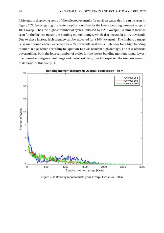
84 CHAPTER 7. PRESENTATION AND EVALUATION OF RESULTS
A histogram displaying some of the selected overpulls for an 80 m water depth can be seen in
Figure 7.22. Investigating this water depth shows that for the lowest bending moment range, a
100 t overpull has the highest number of cycles, followed by a 25 t overpull. A similar trend is
seen for the highest maximum bending moment range, which also occurs for a 100 t overpull.
Due to these factors, high damage can be expected for a 100 t overpull. The highest damage
is, as mentioned earlier, expected for a 25 t overpull, as it has a high peak for a high bending
moment range, which according to Equation 4.12 will result in high damage. The case of the 80
t overpull has both the lowest number of cycles for the lowest bending moment range, lowest
maximum bending moment range and the lowest peak, thus it is expected the smallest amount
of damage for this overpull.
Figure 7.22: Bending moment histogram: Overpull variation - 80 m
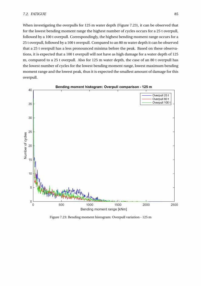
7.2. FATIGUE 85
When investigating the overpulls for 125 m water depth (Figure 7.23), it can be observed that
for the lowest bending moment range the highest number of cycles occurs for a 25 t overpull,
followed by a 100 t overpull. Correspondingly, the highest bending moment range occurs for a
25 t overpull, followed by a 100 t overpull. Compared to an 80 m water depth it can be observed
that a 25 t overpull has a less pronounced minima before the peak. Based on these observa-
tions, it is expected that a 100 t overpull will not have as high damage for a water depth of 125
m, compared to a 25 t overpull. Also for 125 m water depth, the case of an 80 t overpull has
the lowest number of cycles for the lowest bending moment range, lowest maximum bending
moment range and the lowest peak, thus it is expected the smallest amount of damage for this
overpull.
Figure 7.23: Bending moment histogram: Overpull variation - 125 m
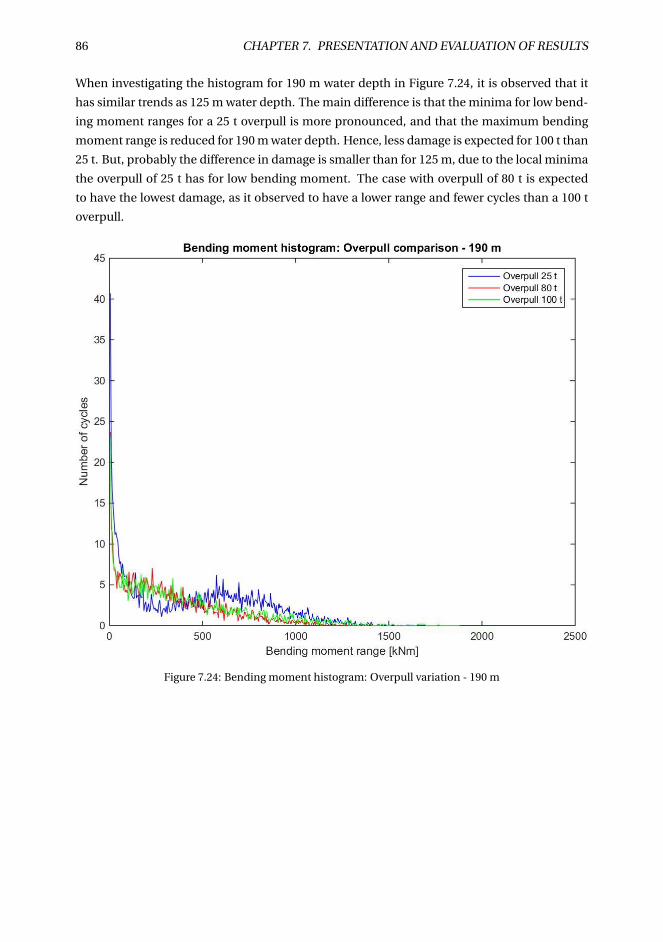
86 CHAPTER 7. PRESENTATION AND EVALUATION OF RESULTS
When investigating the histogram for 190 m water depth in Figure 7.24, it is observed that it
has similar trends as 125 m water depth. The main difference is that the minima for low bend-
ing moment ranges for a 25 t overpull is more pronounced, and that the maximum bending
moment range is reduced for 190 m water depth. Hence, less damage is expected for 100 t than
25 t. But, probably the difference in damage is smaller than for 125 m, due to the local minima
the overpull of 25 t has for low bending moment. The case with overpull of 80 t is expected
to have the lowest damage, as it observed to have a lower range and fewer cycles than a 100 t
overpull.
Figure 7.24: Bending moment histogram: Overpull variation - 190 m
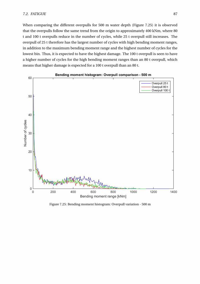
7.2. FATIGUE 87
When comparing the different overpulls for 500 m water depth (Figure 7.25) it is observed
that the overpulls follow the same trend from the origin to approximately 400 kNm, where 80
t and 100 t overpulls reduce in the number of cycles, while 25 t overpull still increases. The
overpull of 25 t therefore has the largest number of cycles with high bending moment ranges,
in addition to the maximum bending moment range and the highest number of cycles for the
lowest bin. Thus, it is expected to have the highest damage. The 100 t overpull is seen to have
a higher number of cycles for the high bending moment ranges than an 80 t overpull, which
means that higher damage is expected for a 100 t overpull than an 80 t.
Figure 7.25: Bending moment histogram: Overpull variation - 500 m
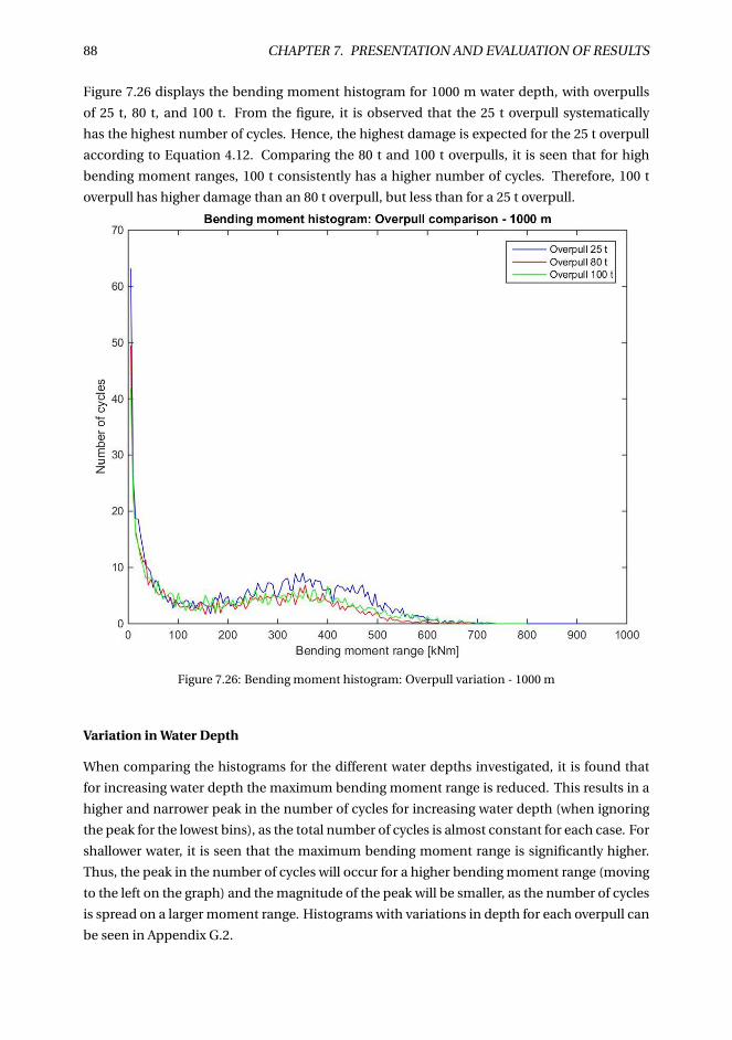
88 CHAPTER 7. PRESENTATION AND EVALUATION OF RESULTS
Figure 7.26 displays the bending moment histogram for 1000 m water depth, with overpulls
of 25 t, 80 t, and 100 t. From the figure, it is observed that the 25 t overpull systematically
has the highest number of cycles. Hence, the highest damage is expected for the 25 t overpull
according to Equation 4.12. Comparing the 80 t and 100 t overpulls, it is seen that for high
bending moment ranges, 100 t consistently has a higher number of cycles. Therefore, 100 t
overpull has higher damage than an 80 t overpull, but less than for a 25 t overpull.
Figure 7.26: Bending moment histogram: Overpull variation - 1000 m
Variation in Water Depth
When comparing the histograms for the different water depths investigated, it is found that
for increasing water depth the maximum bending moment range is reduced. This results in a
higher and narrower peak in the number of cycles for increasing water depth (when ignoring
the peak for the lowest bins), as the total number of cycles is almost constant for each case. For
shallower water, it is seen that the maximum bending moment range is significantly higher.
Thus, the peak in the number of cycles will occur for a higher bending moment range (moving
to the left on the graph) and the magnitude of the peak will be smaller, as the number of cycles
is spread on a larger moment range. Histograms with variations in depth for each overpull can
be seen in Appendix G.2.
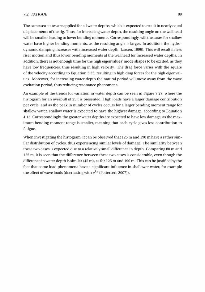
7.2. FATIGUE 89
The same sea states are applied for all water depths, which is expected to result in nearly equal
displacements of the rig. Thus, for increasing water depth, the resulting angle on the wellhead
will be smaller, leading to lower bending moments. Correspondingly, will the cases for shallow
water have higher bending moments, as the resulting angle is larger. In addition, the hydro-
dynamic damping increases with increased water depth (Larsen; 1996). This will result in less
riser motion and thus lower bending moments at the wellhead for increased water depths. In
addition, there is not enough time for the high eigenvalues’ mode shapes to be excited, as they
have low frequencies, thus resulting in high velocity. The drag force varies with the square
of the velocity according to Equation 3.33, resulting in high drag forces for the high eigenval-
ues. Moreover, for increasing water depth the natural period will move away from the wave
excitation period, thus reducing resonance phenomena.
An example of the trends for variation in water depth can be seen in Figure 7.27, where the
histogram for an overpull of 25 t is presented. High loads have a larger damage contribution
per cycle, and as the peak in number of cycles occurs for a larger bending moment range for
shallow water, shallow water is expected to have the highest damage, according to Equation
4.12. Correspondingly, the greater water depths are expected to have low damage, as the max-
imum bending moment range is smaller, meaning that each cycle gives less contribution to
fatigue.
When investigating the histogram, it can be observed that 125 m and 190 m have a rather sim-
ilar distribution of cycles, thus experiencing similar levels of damage. The similarity between
these two cases is expected due to a relatively small difference in depth. Comparing 80 m and
125 m, it is seen that the difference between these two cases is considerable, even though the
difference in water depth is similar (45 m), as for 125 m and 190 m. This can be justified by the
fact that some load phenomena have a significant influence in shallower water, for example
the effect of wave loads (decreasing with ekz (Pettersen; 2007)).
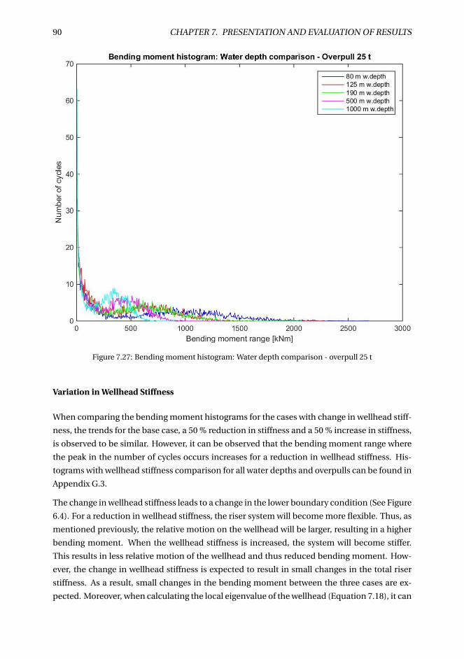
90 CHAPTER 7. PRESENTATION AND EVALUATION OF RESULTS
Figure 7.27: Bending moment histogram: Water depth comparison - overpull 25 t
Variation in Wellhead Stiffness
When comparing the bending moment histograms for the cases with change in wellhead stiff-
ness, the trends for the base case, a 50 % reduction in stiffness and a 50 % increase in stiffness,
is observed to be similar. However, it can be observed that the bending moment range where
the peak in the number of cycles occurs increases for a reduction in wellhead stiffness. His-
tograms with wellhead stiffness comparison for all water depths and overpulls can be found in
Appendix G.3.
The change in wellhead stiffness leads to a change in the lower boundary condition (See Figure
6.4). For a reduction in wellhead stiffness, the riser system will become more flexible. Thus, as
mentioned previously, the relative motion on the wellhead will be larger, resulting in a higher
bending moment. When the wellhead stiffness is increased, the system will become stiffer.
This results in less relative motion of the wellhead and thus reduced bending moment. How-
ever, the change in wellhead stiffness is expected to result in small changes in the total riser
stiffness. As a result, small changes in the bending moment between the three cases are ex-
pected. Moreover, when calculating the local eigenvalue of the wellhead (Equation 7.18), it can
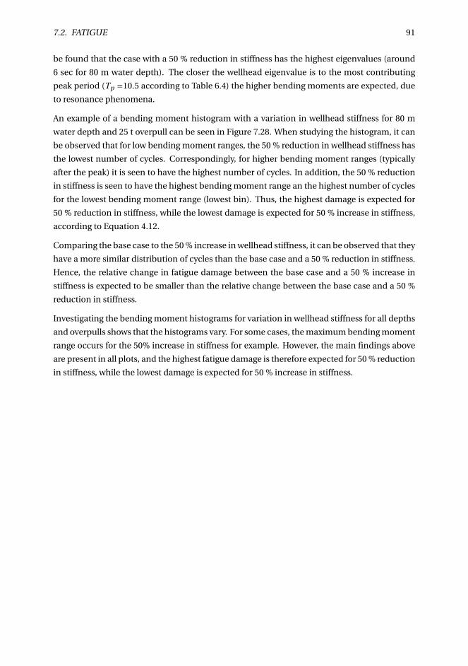
7.2. FATIGUE 91
be found that the case with a 50 % reduction in stiffness has the highest eigenvalues (around
6 sec for 80 m water depth). The closer the wellhead eigenvalue is to the most contributing
peak period (Tp =10.5 according to Table 6.4) the higher bending moments are expected, due
to resonance phenomena.
An example of a bending moment histogram with a variation in wellhead stiffness for 80 m
water depth and 25 t overpull can be seen in Figure 7.28. When studying the histogram, it can
be observed that for low bending moment ranges, the 50 % reduction in wellhead stiffness has
the lowest number of cycles. Correspondingly, for higher bending moment ranges (typically
after the peak) it is seen to have the highest number of cycles. In addition, the 50 % reduction
in stiffness is seen to have the highest bending moment range an the highest number of cycles
for the lowest bending moment range (lowest bin). Thus, the highest damage is expected for
50 % reduction in stiffness, while the lowest damage is expected for 50 % increase in stiffness,
according to Equation 4.12.
Comparing the base case to the 50 % increase in wellhead stiffness, it can be observed that they
have a more similar distribution of cycles than the base case and a 50 % reduction in stiffness.
Hence, the relative change in fatigue damage between the base case and a 50 % increase in
stiffness is expected to be smaller than the relative change between the base case and a 50 %
reduction in stiffness.
Investigating the bending moment histograms for variation in wellhead stiffness for all depths
and overpulls shows that the histograms vary. For some cases, the maximum bending moment
range occurs for the 50% increase in stiffness for example. However, the main findings above
are present in all plots, and the highest fatigue damage is therefore expected for 50 % reduction
in stiffness, while the lowest damage is expected for 50 % increase in stiffness.
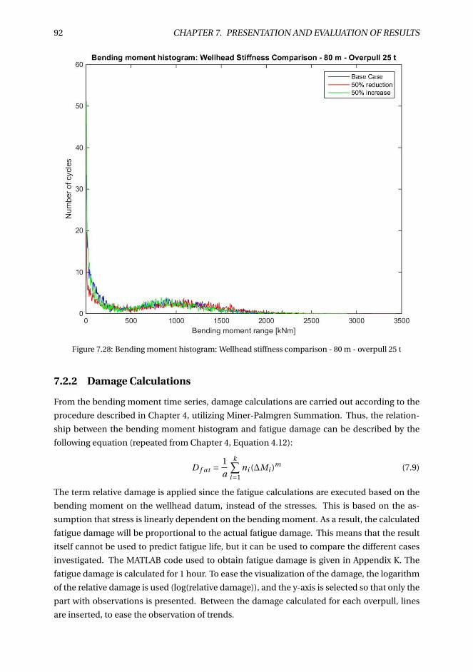
92 CHAPTER 7. PRESENTATION AND EVALUATION OF RESULTS
Figure 7.28: Bending moment histogram: Wellhead stiffness comparison - 80 m - overpull 25 t
7.2.2 Damage Calculations
From the bending moment time series, damage calculations are carried out according to the
procedure described in Chapter 4, utilizing Miner-Palmgren Summation. Thus, the relation-
ship between the bending moment histogram and fatigue damage can be described by the
following equation (repeated from Chapter 4, Equation 4.12):
D f at =1
a
k∑i=1
ni (∆Mi )m (7.9)
The term relative damage is applied since the fatigue calculations are executed based on the
bending moment on the wellhead datum, instead of the stresses. This is based on the as-
sumption that stress is linearly dependent on the bending moment. As a result, the calculated
fatigue damage will be proportional to the actual fatigue damage. This means that the result
itself cannot be used to predict fatigue life, but it can be used to compare the different cases
investigated. The MATLAB code used to obtain fatigue damage is given in Appendix K. The
fatigue damage is calculated for 1 hour. To ease the visualization of the damage, the logarithm
of the relative damage is used (log(relative damage)), and the y-axis is selected so that only the
part with observations is presented. Between the damage calculated for each overpull, lines
are inserted, to ease the observation of trends.
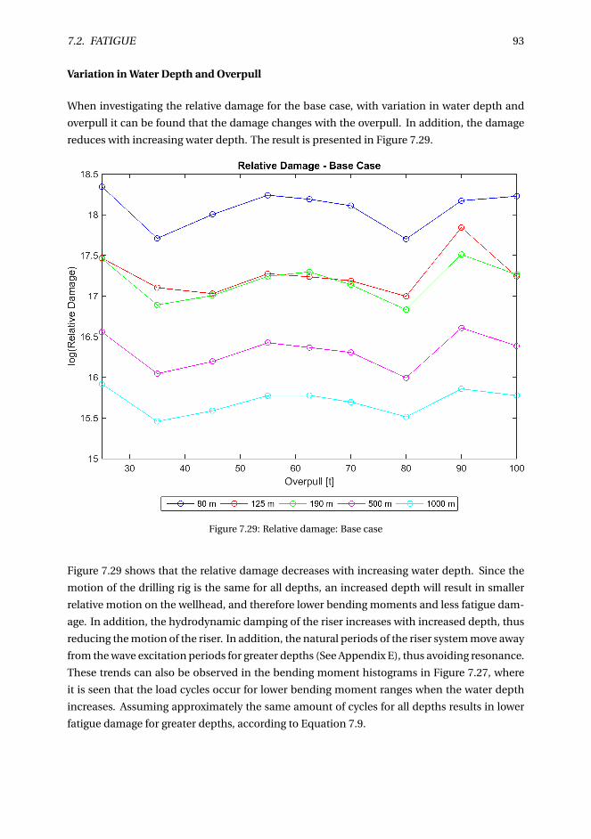
7.2. FATIGUE 93
Variation in Water Depth and Overpull
When investigating the relative damage for the base case, with variation in water depth and
overpull it can be found that the damage changes with the overpull. In addition, the damage
reduces with increasing water depth. The result is presented in Figure 7.29.
Figure 7.29: Relative damage: Base case
Figure 7.29 shows that the relative damage decreases with increasing water depth. Since the
motion of the drilling rig is the same for all depths, an increased depth will result in smaller
relative motion on the wellhead, and therefore lower bending moments and less fatigue dam-
age. In addition, the hydrodynamic damping of the riser increases with increased depth, thus
reducing the motion of the riser. In addition, the natural periods of the riser system move away
from the wave excitation periods for greater depths (See Appendix E), thus avoiding resonance.
These trends can also be observed in the bending moment histograms in Figure 7.27, where
it is seen that the load cycles occur for lower bending moment ranges when the water depth
increases. Assuming approximately the same amount of cycles for all depths results in lower
fatigue damage for greater depths, according to Equation 7.9.
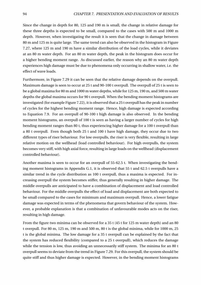
94 CHAPTER 7. PRESENTATION AND EVALUATION OF RESULTS
Since the change in depth for 80, 125 and 190 m is small, the change in relative damage for
these three depths is expected to be small, compared to the cases with 500 m and 1000 m
depth. However, when investigating the result it is seen that the change in damage between
80 m and 125 m is quite large. The same trend can also be observed in the histogram in Figure
7.27, where 125 m and 190 m have a similar distribution of the load cycles, while it deviates
at an 80 m water depth. For an 80 m water depth, the peak in the histogram does occur for
a higher bending moment range. As discussed earlier, the reason why an 80 m water depth
experiences high damage must be due to phenomena only occurring in shallow water, i.e. the
effect of wave loads.
Furthermore, in Figure 7.29 it can be seen that the relative damage depends on the overpull.
Maximum damage is seen to occur at 25 t and 90-100 t overpull. The overpull of 25 t is seen to
be a global maxima for 80 m and 1000 m water depths, while for 125 m, 190 m, and 500 m water
depths the global maxima occurs for 90 t overpull. When the bending moment histograms are
investigated (for example Figure 7.22), it is observed that a 25 t overpull has the peak in number
of cycles for the highest bending moment range. Hence, high damage is expected according
to Equation 7.9. For an overpull of 90-100 t high damage is also observed. In the bending
moment histograms, an overpull of 100 t is seen as having a larger number of cycles for high
bending moment ranges than 80 t, thus experiencing higher damage for a 100 t overpull than
a 80 t overpull. Even though both 25 t and 100 t have high damage, they occur due to two
different types of riser behaviour. For low overpulls, the riser is very flexible, resulting in large
relative motion on the wellhead (load controlled behaviour). For high overpulls, the system
becomes very stiff, with high axial force, resulting in large loads on the wellhead (displacement
controlled behaviour).
Another maxima is seen to occur for an overpull of 55-62.5 t. When investigating the bend-
ing moment histograms in Appendix G.1, it is observed that 55 t and 62.5 t overpulls have a
similar trend in the cycle distribution as 100 t overpull, thus a maxima is expected. For in-
creasing overpull the system becomes stiffer, thus generally resulting in higher damage. The
middle overpulls are anticipated to have a combination of displacement and load controlled
behaviour. For the middle overpulls the effect of load and displacement are both expected to
be small compared to the cases for minimum and maximum overpull. Hence, a lower fatigue
damage was expected in terms of the phenomena that govern behaviour of the system. How-
ever, a probable explanation is that a combination of unfavourable modes acts on the riser,
resulting in high damage.
From the figure two minima can be observed for a 35 t (45 t for 125 m water depth) and an 80
t overpull. For 80 m, 125 m, 190 m and 500 m, 80 t is the global minima, while for 1000 m, 25
t is the global minima. The low damage for a 35 t overpull can be explained by the fact that
the system has reduced flexibility (compared to a 25 t overpull), which reduces the damage
while the tension is low, thus avoiding an unnecessarily stiff system. The minima for an 80 t
overpull seems to deviate from the trend in Figure 7.29. For this overpull, the system should be
quite stiff and thus higher damage is expected. However, in the bending moment histograms
7.2. FATIGUE 95
it is observed that an 80 t overpull has a lower peak than a 100 t overpull, and also has a lower
maximum bending moment range. Thus, it is expected based on the histogram. Also this
minima can be explained by a combination of favourable modes acting on the riser, resulting
in low damage.
The change in damage due to overpull can also be seen in Table 7.4. It is observed that the
change in damage from the minimum to the maximum damage is high. In addition, it is ob-
served that the actual maximum fatigue damage is 30-300 % higher than the fatigue damage
for the maximum tension (100 t overpull). Hence, using the maximum tension as suggested in
the JIP (DNV; 2011), can result in a significant underestimation of fatigue. Correspondingly, it
is observed that the minimum fatigue damage is 40-70 % lower than the fatigue damage for a
100 t overpull.Table 7.4: Change in damage due to overpull
Water Depth 80 m 125 m 190 m 500 m 1000 m
Change: min-max 340.8 % 602.1 % 378.6 % 311.4 % 187.5 %
Change: 100 t overpull to min -70.3 % -43.1 % -63.0 % -59.5 % -51.9 %
Change: 100 t overpull to max 31.0 % 299.3 % 77.0 % 66.7 % 38.2 %
The size and weight of the BOP was identified as the main factor for fatigue damage in an
analysis by Greene and Williams (2012b)(see Chapter 1). As a basis for comparison, changing
the BOP size and weight (3rd vs. 6th generation drilling rig BOP) results in a fatigue change of
approximately 1500 % (Williams and Greene; 2012b). The maximum change in damage for a
variation in tension is observed to be 600 %, thus BOP is seen to be a more important factor.
However, for some situations the rig and equipment is already selected (for example the BOP).
Then, only changes in the operation of the drilling rig are possible. Hence, tension is one of
the few parameters it is possible to change. Therefore it is still important to examine tension
as part of the fatigue analysis.
In the analysis by Greene and Williams (2012b) a variation in tension was also investigated.
For a 3rd generation drilling rig, the damage was seen to increase with 133 % for an increase in
overpull from 50 to 200 kips. Kips is defined as a 1000-pound-force, thus a change in overpull
from 50 to 200 kips, equals a change of 23-90 t overpull. The change observed by Williams and
Greene is smaller than the change observed in this study (Table 7.4). However, the damage
will also depend on the other parameters used in the analysis, like water depth, environmental
conditions, and drilling rig. The numbers are therefore not directly comparable.
96 CHAPTER 7. PRESENTATION AND EVALUATION OF RESULTS
Variation in Wellhead Stiffness
When comparing the relative damage for the different wellhead stiffnesses, it is observed that
the highest fatigue damage occurs for a 50 % reduction in stiffness, and the lowest damage for
a 50 % increase in stiffness. It can also be seen that the base case and a 50% increase in stiffness
are more similar in magnitude than the base case and a 50% increase in damage. The results
are visualized in Figure 7.30, where the relative damage for the base case, a 50 % reduction in
stiffness, and a 50 % increase in stiffness are presented, for all water depths and overpulls. In
addition, damage plots where each of the three stiffness cases is presented separately can be
found in Appendix H.
Figure 7.30: Relative damage: Comparison of change in WH stiffness
The reduction in wellhead stiffness leads to a more flexible system, with larger motions of
the wellhead, thus it experiences higher fatigue damage. This also corresponds with the his-
tograms in Section 7.2.1, where the case of a 50 % reduction in stiffness has the highest number
of cycles for high bending moment ranges. Moreover, the maximum bending moment range is
highest for the case with a 50 % reduction in stiffness. According to Equation 7.9, high fatigue
damage should be expected. On the contrary, the case with a 50 % increase in stiffness ex-
periences the lowest amount of fatigue damage since it contain fewer cycles for high bending
moment ranges than both the 50 % reduction in stiffness and the base case.
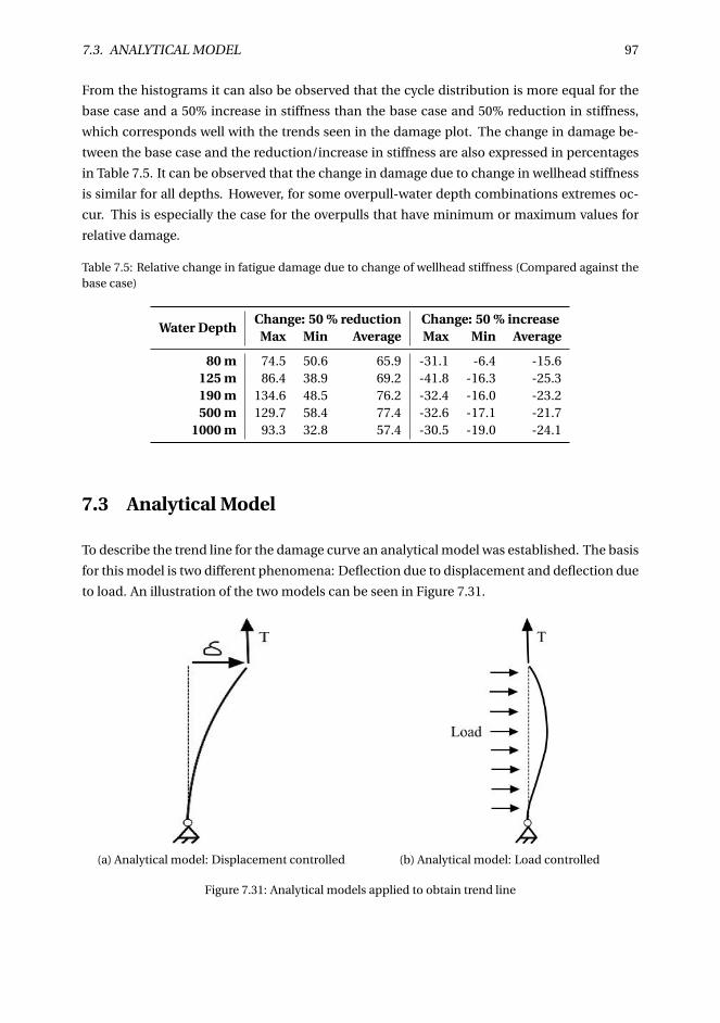
7.3. ANALYTICAL MODEL 97
From the histograms it can also be observed that the cycle distribution is more equal for the
base case and a 50% increase in stiffness than the base case and 50% reduction in stiffness,
which corresponds well with the trends seen in the damage plot. The change in damage be-
tween the base case and the reduction/increase in stiffness are also expressed in percentages
in Table 7.5. It can be observed that the change in damage due to change in wellhead stiffness
is similar for all depths. However, for some overpull-water depth combinations extremes oc-
cur. This is especially the case for the overpulls that have minimum or maximum values for
relative damage.
Table 7.5: Relative change in fatigue damage due to change of wellhead stiffness (Compared against thebase case)
Water DepthChange: 50 % reduction Change: 50 % increase
Max Min Average Max Min Average
80 m 74.5 50.6 65.9 -31.1 -6.4 -15.6125 m 86.4 38.9 69.2 -41.8 -16.3 -25.3190 m 134.6 48.5 76.2 -32.4 -16.0 -23.2500 m 129.7 58.4 77.4 -32.6 -17.1 -21.7
1000 m 93.3 32.8 57.4 -30.5 -19.0 -24.1
7.3 Analytical Model
To describe the trend line for the damage curve an analytical model was established. The basis
for this model is two different phenomena: Deflection due to displacement and deflection due
to load. An illustration of the two models can be seen in Figure 7.31.
(a) Analytical model: Displacement controlled (b) Analytical model: Load controlled
Figure 7.31: Analytical models applied to obtain trend line
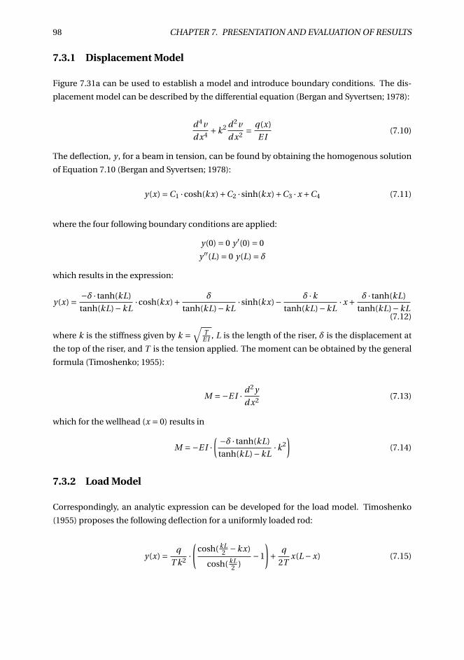
98 CHAPTER 7. PRESENTATION AND EVALUATION OF RESULTS
7.3.1 Displacement Model
Figure 7.31a can be used to establish a model and introduce boundary conditions. The dis-
placement model can be described by the differential equation (Bergan and Syvertsen; 1978):
d 4v
d x4 +k2 d 2v
d x2 = q(x)
E I(7.10)
The deflection, y , for a beam in tension, can be found by obtaining the homogenous solution
of Equation 7.10 (Bergan and Syvertsen; 1978):
y(x) =C1 ·cosh(kx)+C2 · sinh(kx)+C3 · x +C4 (7.11)
where the four following boundary conditions are applied:
y(0) = 0 y ′(0) = 0
y ′′(L) = 0 y(L) = δwhich results in the expression:
y(x) = −δ · tanh(kL)
tanh(kL)−kL·cosh(kx)+ δ
tanh(kL)−kL·sinh(kx)− δ ·k
tanh(kL)−kL·x + δ · tanh(kL)
tanh(kL)−kL(7.12)
where k is the stiffness given by k =√
TE I , L is the length of the riser, δ is the displacement at
the top of the riser, and T is the tension applied. The moment can be obtained by the general
formula (Timoshenko; 1955):
M =−E I · d 2 y
d x2 (7.13)
which for the wellhead (x = 0) results in
M =−E I ·( −δ · tanh(kL)
tanh(kL)−kL·k2
)(7.14)
7.3.2 Load Model
Correspondingly, an analytic expression can be developed for the load model. Timoshenko
(1955) proposes the following deflection for a uniformly loaded rod:
y(x) = q
T k2 ·(
cosh( kL2 −kx)
cosh( kL2 )
−1
)+ q
2Tx(L−x) (7.15)
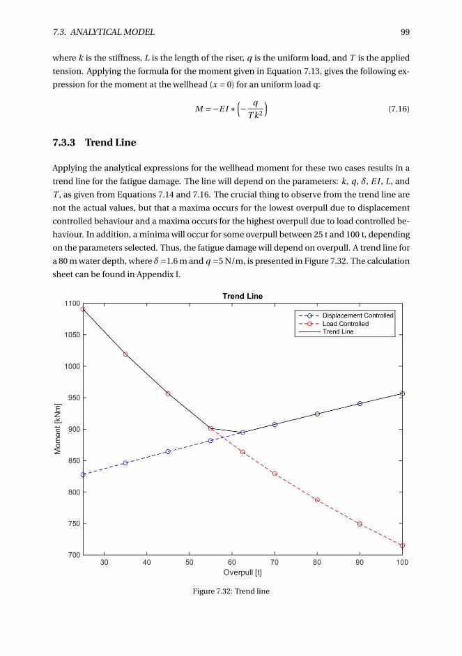
7.3. ANALYTICAL MODEL 99
where k is the stiffness, L is the length of the riser, q is the uniform load, and T is the applied
tension. Applying the formula for the moment given in Equation 7.13, gives the following ex-
pression for the moment at the wellhead (x = 0) for an uniform load q:
M =−E I ∗(− q
T k2
)(7.16)
7.3.3 Trend Line
Applying the analytical expressions for the wellhead moment for these two cases results in a
trend line for the fatigue damage. The line will depend on the parameters: k, q , δ, E I , L, and
T , as given from Equations 7.14 and 7.16. The crucial thing to observe from the trend line are
not the actual values, but that a maxima occurs for the lowest overpull due to displacement
controlled behaviour and a maxima occurs for the highest overpull due to load controlled be-
haviour. In addition, a minima will occur for some overpull between 25 t and 100 t, depending
on the parameters selected. Thus, the fatigue damage will depend on overpull. A trend line for
a 80 m water depth, where δ=1.6 m and q =5 N/m, is presented in Figure 7.32. The calculation
sheet can be found in Appendix I.
Figure 7.32: Trend line
100 CHAPTER 7. PRESENTATION AND EVALUATION OF RESULTS
When comparing the trend line in Figure 7.32 and the damage plots in Section 7.2.2, it can
be observed that these do not correlate perfectly. In general, it fits for the overpulls with the
highest damage. For the lowest overpull, the damage is load controlled, and for the highest
overpull it is displacement controlled. However, the middle overpulls can be observed to have
some deviation between the trend line and the damage plots. This can especially be observed
in the case with an 80 t overpull. To investigate the mechanisms behind these deviations from
the trend line a sensitivity study is carried out and presented in Section 7.4. Nevertheless, there
are many effects included in the dynamic analysis that are not accounted for in the simplified
analytical model used to establish the trend line. This is one possible reason for the deviation
between the computed relative damage and the expected trend line.
7.4 Sensitivity Studies
According to the given theory, as described in Section 7.3, it is expected that the relative dam-
age curve should resemble the proposed trend line (Figure 7.32). However, as seen in for exam-
ple Figure 7.30, there is a deviation in the results for some of the middle overpulls, especially
at 80 t. As this is somewhat unexpected, several possibilities are investigated to explain the
results obtained and to better understand the phenomena. Unless otherwise noted, the inves-
tigations are conducted for an 80 m water depth.
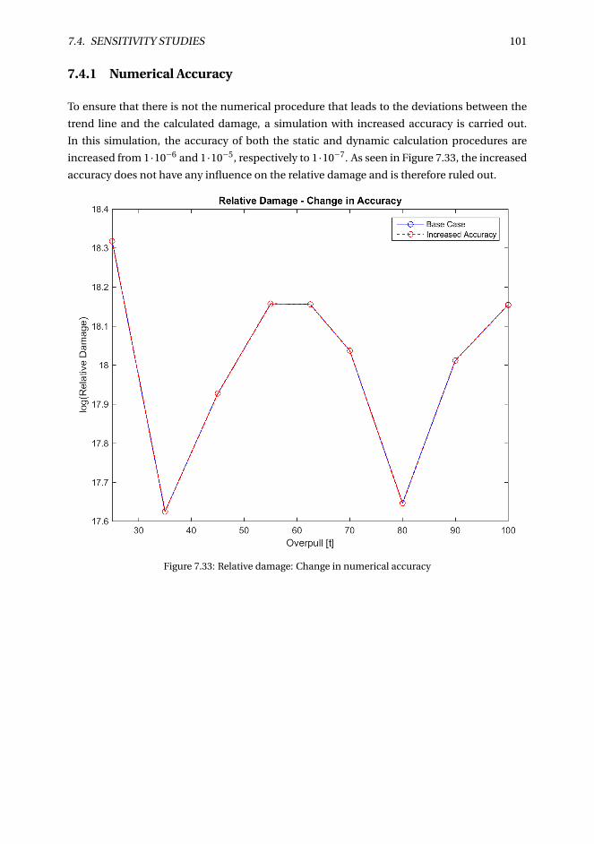
7.4. SENSITIVITY STUDIES 101
7.4.1 Numerical Accuracy
To ensure that there is not the numerical procedure that leads to the deviations between the
trend line and the calculated damage, a simulation with increased accuracy is carried out.
In this simulation, the accuracy of both the static and dynamic calculation procedures are
increased from 1·10−6 and 1·10−5, respectively to 1 ·10−7. As seen in Figure 7.33, the increased
accuracy does not have any influence on the relative damage and is therefore ruled out.
Figure 7.33: Relative damage: Change in numerical accuracy
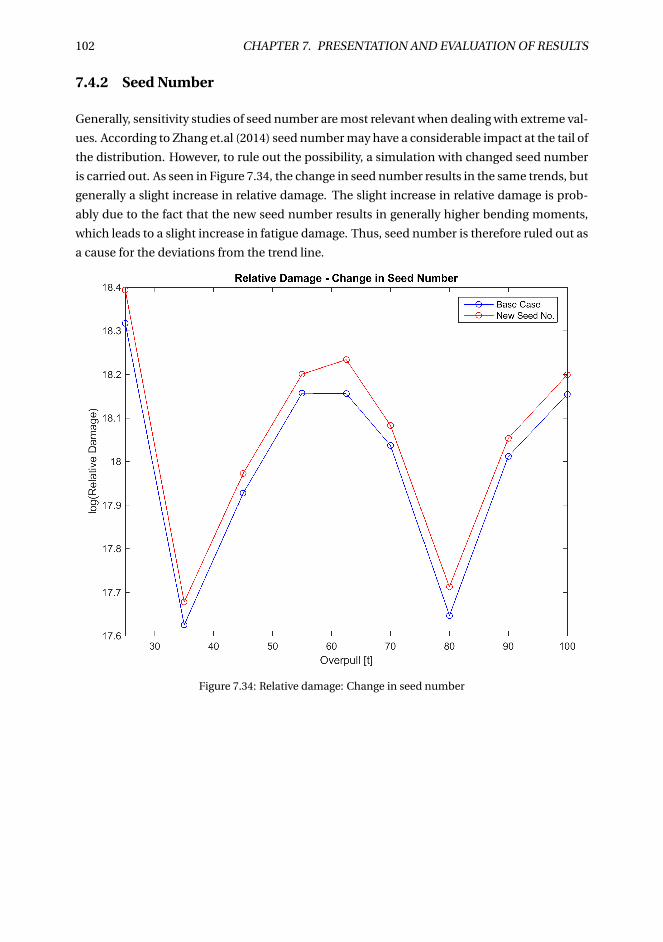
102 CHAPTER 7. PRESENTATION AND EVALUATION OF RESULTS
7.4.2 Seed Number
Generally, sensitivity studies of seed number are most relevant when dealing with extreme val-
ues. According to Zhang et.al (2014) seed number may have a considerable impact at the tail of
the distribution. However, to rule out the possibility, a simulation with changed seed number
is carried out. As seen in Figure 7.34, the change in seed number results in the same trends, but
generally a slight increase in relative damage. The slight increase in relative damage is prob-
ably due to the fact that the new seed number results in generally higher bending moments,
which leads to a slight increase in fatigue damage. Thus, seed number is therefore ruled out as
a cause for the deviations from the trend line.
Figure 7.34: Relative damage: Change in seed number
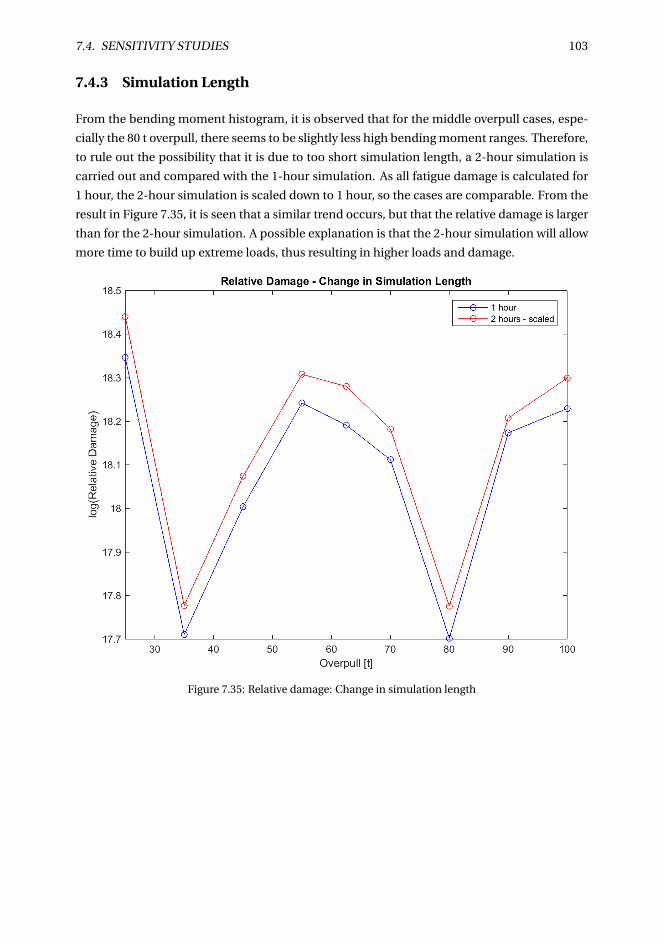
7.4. SENSITIVITY STUDIES 103
7.4.3 Simulation Length
From the bending moment histogram, it is observed that for the middle overpull cases, espe-
cially the 80 t overpull, there seems to be slightly less high bending moment ranges. Therefore,
to rule out the possibility that it is due to too short simulation length, a 2-hour simulation is
carried out and compared with the 1-hour simulation. As all fatigue damage is calculated for
1 hour, the 2-hour simulation is scaled down to 1 hour, so the cases are comparable. From the
result in Figure 7.35, it is seen that a similar trend occurs, but that the relative damage is larger
than for the 2-hour simulation. A possible explanation is that the 2-hour simulation will allow
more time to build up extreme loads, thus resulting in higher loads and damage.
Figure 7.35: Relative damage: Change in simulation length
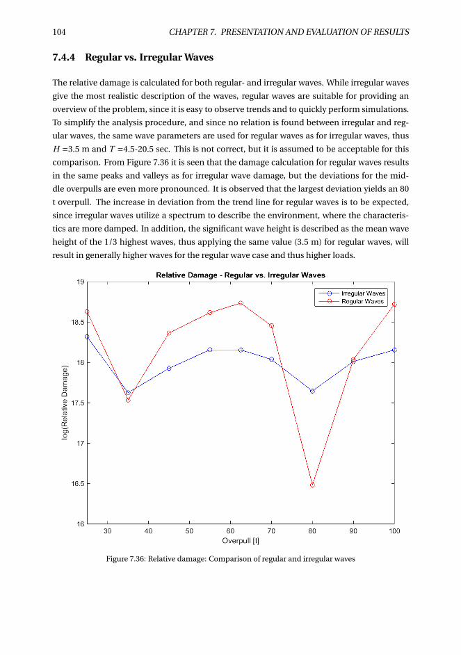
104 CHAPTER 7. PRESENTATION AND EVALUATION OF RESULTS
7.4.4 Regular vs. Irregular Waves
The relative damage is calculated for both regular- and irregular waves. While irregular waves
give the most realistic description of the waves, regular waves are suitable for providing an
overview of the problem, since it is easy to observe trends and to quickly perform simulations.
To simplify the analysis procedure, and since no relation is found between irregular and reg-
ular waves, the same wave parameters are used for regular waves as for irregular waves, thus
H =3.5 m and T =4.5-20.5 sec. This is not correct, but it is assumed to be acceptable for this
comparison. From Figure 7.36 it is seen that the damage calculation for regular waves results
in the same peaks and valleys as for irregular wave damage, but the deviations for the mid-
dle overpulls are even more pronounced. It is observed that the largest deviation yields an 80
t overpull. The increase in deviation from the trend line for regular waves is to be expected,
since irregular waves utilize a spectrum to describe the environment, where the characteris-
tics are more damped. In addition, the significant wave height is described as the mean wave
height of the 1/3 highest waves, thus applying the same value (3.5 m) for regular waves, will
result in generally higher waves for the regular wave case and thus higher loads.
Figure 7.36: Relative damage: Comparison of regular and irregular waves
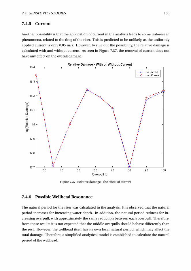
7.4. SENSITIVITY STUDIES 105
7.4.5 Current
Another possibility is that the application of current in the analysis leads to some unforeseen
phenomena, related to the drag of the riser. This is predicted to be unlikely, as the uniformly
applied current is only 0.05 m/s. However, to rule out the possibility, the relative damage is
calculated with and without current. As seen in Figure 7.37, the removal of current does not
have any effect on the overall damage.
Figure 7.37: Relative damage: The effect of current
7.4.6 Possible Wellhead Resonance
The natural period for the riser was calculated in the analysis. It is observed that the natural
period increases for increasing water depth. In addition, the natural period reduces for in-
creasing overpull, with approximately the same reduction between each overpull. Therefore,
from these results it is not expected that the middle overpulls should behave differently than
the rest. However, the wellhead itself has its own local natural period, which may affect the
total damage. Therefore, a simplified analytical model is established to calculate the natural
period of the wellhead.
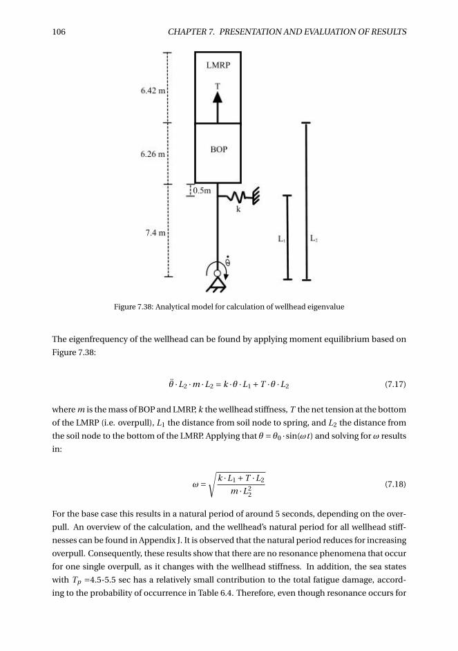
106 CHAPTER 7. PRESENTATION AND EVALUATION OF RESULTS
Figure 7.38: Analytical model for calculation of wellhead eigenvalue
The eigenfrequency of the wellhead can be found by applying moment equilibrium based on
Figure 7.38:
θ ·L2 ·m ·L2 = k ·θ ·L1 +T ·θ ·L2 (7.17)
where m is the mass of BOP and LMRP, k the wellhead stiffness, T the net tension at the bottom
of the LMRP (i.e. overpull), L1 the distance from soil node to spring, and L2 the distance from
the soil node to the bottom of the LMRP. Applying that θ = θ0 ·sin(ωt ) and solving for ω results
in:
ω=√
k ·L1 +T ·L2
m ·L22
(7.18)
For the base case this results in a natural period of around 5 seconds, depending on the over-
pull. An overview of the calculation, and the wellhead’s natural period for all wellhead stiff-
nesses can be found in Appendix J. It is observed that the natural period reduces for increasing
overpull. Consequently, these results show that there are no resonance phenomena that occur
for one single overpull, as it changes with the wellhead stiffness. In addition, the sea states
with Tp =4.5-5.5 sec has a relatively small contribution to the total fatigue damage, accord-
ing to the probability of occurrence in Table 6.4. Therefore, even though resonance occurs for
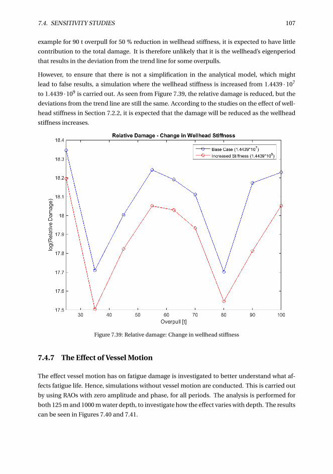
7.4. SENSITIVITY STUDIES 107
example for 90 t overpull for 50 % reduction in wellhead stiffness, it is expected to have little
contribution to the total damage. It is therefore unlikely that it is the wellhead’s eigenperiod
that results in the deviation from the trend line for some overpulls.
However, to ensure that there is not a simplification in the analytical model, which might
lead to false results, a simulation where the wellhead stiffness is increased from 1.4439 · 107
to 1.4439 ·109 is carried out. As seen from Figure 7.39, the relative damage is reduced, but the
deviations from the trend line are still the same. According to the studies on the effect of well-
head stiffness in Section 7.2.2, it is expected that the damage will be reduced as the wellhead
stiffness increases.
Figure 7.39: Relative damage: Change in wellhead stiffness
7.4.7 The Effect of Vessel Motion
The effect vessel motion has on fatigue damage is investigated to better understand what af-
fects fatigue life. Hence, simulations without vessel motion are conducted. This is carried out
by using RAOs with zero amplitude and phase, for all periods. The analysis is performed for
both 125 m and 1000 m water depth, to investigate how the effect varies with depth. The results
can be seen in Figures 7.40 and 7.41.
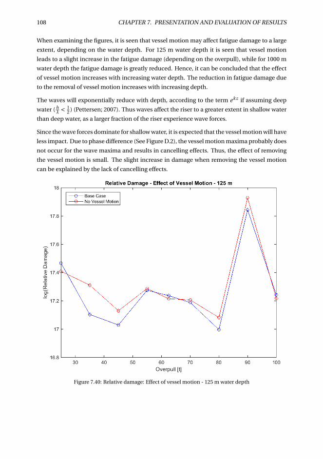
108 CHAPTER 7. PRESENTATION AND EVALUATION OF RESULTS
When examining the figures, it is seen that vessel motion may affect fatigue damage to a large
extent, depending on the water depth. For 125 m water depth it is seen that vessel motion
leads to a slight increase in the fatigue damage (depending on the overpull), while for 1000 m
water depth the fatigue damage is greatly reduced. Hence, it can be concluded that the effect
of vessel motion increases with increasing water depth. The reduction in fatigue damage due
to the removal of vessel motion increases with increasing depth.
The waves will exponentially reduce with depth, according to the term ekz if assuming deep
water ( hλ < 1
2 ) (Pettersen; 2007). Thus waves affect the riser to a greater extent in shallow water
than deep water, as a larger fraction of the riser experience wave forces.
Since the wave forces dominate for shallow water, it is expected that the vessel motion will have
less impact. Due to phase difference (See Figure D.2), the vessel motion maxima probably does
not occur for the wave maxima and results in cancelling effects. Thus, the effect of removing
the vessel motion is small. The slight increase in damage when removing the vessel motion
can be explained by the lack of cancelling effects.
Figure 7.40: Relative damage: Effect of vessel motion - 125 m water depth
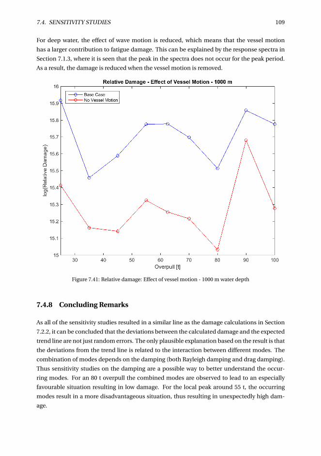
7.4. SENSITIVITY STUDIES 109
For deep water, the effect of wave motion is reduced, which means that the vessel motion
has a larger contribution to fatigue damage. This can be explained by the response spectra in
Section 7.1.3, where it is seen that the peak in the spectra does not occur for the peak period.
As a result, the damage is reduced when the vessel motion is removed.
Figure 7.41: Relative damage: Effect of vessel motion - 1000 m water depth
7.4.8 Concluding Remarks
As all of the sensitivity studies resulted in a similar line as the damage calculations in Section
7.2.2, it can be concluded that the deviations between the calculated damage and the expected
trend line are not just random errors. The only plausible explanation based on the result is that
the deviations from the trend line is related to the interaction between different modes. The
combination of modes depends on the damping (both Rayleigh damping and drag damping).
Thus sensitivity studies on the damping are a possible way to better understand the occur-
ring modes. For an 80 t overpull the combined modes are observed to lead to an especially
favourable situation resulting in low damage. For the local peak around 55 t, the occurring
modes result in a more disadvantageous situation, thus resulting in unexpectedly high dam-
age.
110 CHAPTER 7. PRESENTATION AND EVALUATION OF RESULTS
7.5 Uncertainties
There are many uncertainties related to the global analysis itself and also the assumptions that
will affect the overall fatigue life. However, since the goal of this thesis is to compare different
cases, and the same procedure is used to obtain the result for all cases, these uncertainties and
assumptions are expected to be less important. However, if the goal was to obtain the exact
fatigue life, these uncertainties should be investigated further. Some of the uncertainties will
be presented below:
7.5.1 Modelling
For the calculation of the global response of the drilling riser, a finite element model is used.
The method is well proven, but it is still an approximate method that might lead to uncertain-
ties in the results. The results will depend on the choice of element types, number of elements,
how the non-linearities in the system are modelled and so on. A sensitivity study of the num-
ber of elements is one possible method to assess the uncertainty of the finite element model.
The selection of element type and number of elements in this thesis is based on an example of
a drilling riser given in SIMA/RIFLEX.
Many parts of the drilling riser, especially BOP, LMRP, and wellhead have complex geometries.
For instance, the cross-section will vary with the length. In the global analysis, they are mod-
elled using beam elements with constant cross-section. As mentioned in the introduction,
Holden et al.(2013) stated that wellhead fatigue is among other factors dependent on BOP dy-
namics. It is therefore possible that a more detailed model of the BOP, LMRP, and wellhead
could change the results. However, the master’s thesis by Harildstad and Haukanes (2013)
showed that refining the BOP model had little effect on the overall fatigue damage.
7.5.2 Drag Coefficient
In the analysis, drag coefficients given by Aker Solutions is used. The drag coefficients are given
for the different cross sections of the riser, not taking into account the increased drag due to
kill- and choke lines. A simple solution to this could have been to increase the drag coefficient
for each cross section, but as the influence of the lines is uncertain, it was decided to keep
the original drag coefficient. Especially since the goal of this thesis is a comparison between
different cases, where the same change in drag coefficient therefore would have been applied
to all cases.
In addition, a constant drag coefficient was used for all of the different sea states. In reality,
the drag coefficient is highly dependent on Reynolds number, which again depends on the
velocity at the given location, according to the equation (Pettersen; 2007):
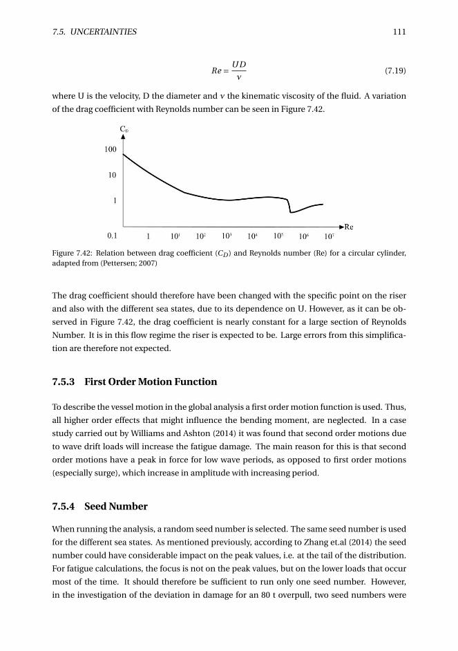
7.5. UNCERTAINTIES 111
Re = U D
ν(7.19)
where U is the velocity, D the diameter and ν the kinematic viscosity of the fluid. A variation
of the drag coefficient with Reynolds number can be seen in Figure 7.42.
Figure 7.42: Relation between drag coefficient (CD ) and Reynolds number (Re) for a circular cylinder,adapted from (Pettersen; 2007)
The drag coefficient should therefore have been changed with the specific point on the riser
and also with the different sea states, due to its dependence on U. However, as it can be ob-
served in Figure 7.42, the drag coefficient is nearly constant for a large section of Reynolds
Number. It is in this flow regime the riser is expected to be. Large errors from this simplifica-
tion are therefore not expected.
7.5.3 First Order Motion Function
To describe the vessel motion in the global analysis a first order motion function is used. Thus,
all higher order effects that might influence the bending moment, are neglected. In a case
study carried out by Williams and Ashton (2014) it was found that second order motions due
to wave drift loads will increase the fatigue damage. The main reason for this is that second
order motions have a peak in force for low wave periods, as opposed to first order motions
(especially surge), which increase in amplitude with increasing period.
7.5.4 Seed Number
When running the analysis, a random seed number is selected. The same seed number is used
for the different sea states. As mentioned previously, according to Zhang et.al (2014) the seed
number could have considerable impact on the peak values, i.e. at the tail of the distribution.
For fatigue calculations, the focus is not on the peak values, but on the lower loads that occur
most of the time. It should therefore be sufficient to run only one seed number. However,
in the investigation of the deviation in damage for an 80 t overpull, two seed numbers were
112 CHAPTER 7. PRESENTATION AND EVALUATION OF RESULTS
compared. As described in Section 7.4.2, a change in seed number leads to increased damage
for all overpulls, but approximately the same relative change. This means that to ensure the
total damage is correct, a sensitivity study on the seed number should be carried out. Applying
only the seed numbers that lead to maximum damage will be too conservative. It is therefore
recommended to change the seed number for each simulation, so that a mean value for the
overall damage is obtained, which is not overly conservative or non-conservative.
7.5.5 Vortex Induced Vibrations
As earlier mentioned, vortex induced vibrations (VIV) are not taken into account for the global
load analysis, as this is not the effect investigated. VIV is a phenomenon where current leads to
vortex shedding on both sides of the cylinder, resulting in vibrations. The vortex shedding fre-
quency increases with increased current velocity (Larsen; 2011). According to Howells (1998),
in deep waters VIV can generate high levels of fatigue damage. Two effects of VIV can be taken
into account for the analysis: Damage from VIV and increased drag force due to VIV (because
of the oscillations) (Larsen; 2011). In this analysis, the drag diameter is increased to include
the effect of increased drag force. The increased damage from VIV is not taken into account.
7.5.6 Environmental Condition
The scatter diagram from the metocean report (Statoil; 2010) is used to select the sea states to
base the simulation on. The challenge is that it is not possible to predict the future exactly, so
the scatter diagram has to be based on historical data and applied statistics. In the resulting
fatigue calculations, there will therefore always be some uncertainties related to if the actual
wave environment will correspond to the assumed (historical) one.
In addition, one wave direction (head sea) and no wave spreading is applied. In recent research
(Holm et al.; 2013) it was found that including wave spreading and water directionality would
decrease the fatigue damage, leading to less conservatism in the analysis. Some wave head-
ings, like beam sea, are expected to result in larger movements, increasing the fatigue dam-
age. But other directions are expected to result in smaller movements, reducing the damage.
Thus the overall damage when including water directionality is expected to decrease. Wave
direction and spreading will also have to be based on historical values, which means that it is
possible to underestimate the fatigue when including these parameters.

7.5. UNCERTAINTIES 113
7.5.7 S-N Curve
The design SN-curve is applied in the fatigue assessment. It is defined as the mean curve
minus two standard deviations and is based on experimental data. According to Almar-Næss
et.al.(1985) there is a significant amount of uncertainty related to the determination of S-N
curves. In addition, classification of each detail, selection of S-N curve and the thickness effect
is uncertain (Almar-Næss et al.; 1985). In general, wellhead fatigue analyses is thus a significant
uncertainty. However, the same S-N curve is applied for all cases investigated, so there might
be an error in magnitude for all cases, but the relative difference between each case should be
the same.
7.5.8 Miner-Palmgren Summation
Miner-Palmgren summation is applied to calculate the fatigue damage, as this is recommended
in the Wellhead Fatigue Analysis Method (DNV; 2011). The method is widely used, but has
three main drawbacks according to Johannesson, Svensson & de Mare (2005), which may lead
to errors when calculating the fatigue damage:
• It does not take into account in which order the load cycles occur, i.e. sequential effects.
• The threshold effects changes when small and large cycles are mixed.
• Residual stresses may remain at a constant amplitude, while relaxing for variable ampli-
tude.
Thus, this may lead to errors in the predicted fatigue life. However, since the same method is
used for all cases compared, the error will be included in all cases.
7.5.9 Block Division
When calculating the fatigue damage, the bending moment histogram is used, adding together
the load from each bin/block which is multiplied with the number of occurrences, according
to Equation 4.12. The histograms are divided in bins of 5000 Nm and to calculate the damage
the upper limit has been used, as a conservative approach. Thus, depending on the load cycles
in each block, the bending moment applied may be overly conservative. This effect magnifies
due the fact that the bending moment range is in the fifth power, since m=5: (∆M)5. How
good the fit is will differ for each simulation. For example, the greater water depths will have
lower maximum bending moment, and correspondingly a lower total number of blocks, than
the shallow water cases. Hence, the block division might lead to more conservative results
for some cases than others. This means that block selection is an uncertainty that relates to
the difference between each case, and is therefore expected to be of most importance of the
presented uncertainties.

114 CHAPTER 7. PRESENTATION AND EVALUATION OF RESULTS
7.6 Limitations
Because of the time available, some limitations had to be made for this thesis. The focus in
this thesis is on global riser dynamics and a relative comparison of fatigue damage. Therefore,
the global load model is simplified to reduce the modelling and computational time. Three
parameters are investigated: Tension/overpull, water depth, and wellhead stiffness. A simpli-
fied tension model is used, applying constant tension. The drilling tube inside the marine riser
is not modelled either. In addition, only one wave and current heading are investigated. It is
found that these were measures that reduced the computational effort while still giving valid
results, since the main goal of this thesis is a relative comparison.
In addition, only waves with a significant wave height of 3.5 m from the scatter diagram were
investigated to reduce the total number of simulations. It is expected that a significant wave
height of 3.5 m will give a good representation for the overall fatigue damage.
As it is the global riser dynamics which are the focus of this thesis, no local analysis of the
wellhead is carried out. The reason is that building a local model of the wellhead from scratch
in FE-software is a very time-demanding task. All fatigue damage is therefore calculated for
the wellhead datum, and not on hotspots on the wellhead itself. This is also the reason why
bending moment are applied in the fatigue calculation instead of stress.
Chapter 8
ConclusionThe objective of this master’s thesis was to investigate the effect tension has on fatigue damage.
The basis for this work is the joint industry project on structural well integrity and the report:
Wellhead Fatigue Analysis Method (DNV; 2011). A fatigue assessment has been carried out for
a variation of overpulls, water depths, and wellhead stiffnesses.
From the global load analysis time series of the bending moment at the wellhead datum was
obtained and histograms produced. It could be observed that the lowest overpull had a high
number of cycles for high bending moment range, thus expecting high damage. In addition,
it was observed that the peak in cycles occurred for higher bending moment range in shallow
water. Hence, it was expected that there would be higher damage for shallow water. When
investigating the variation in wellhead stiffness, it was observed that for a 50 % reduction in
stiffness the peak in the number of cycles occurred for the highest bending moment range,
thus expecting the highest damage.
The damage calculation showed that fatigue damage varies with overpull. The change from
the overpull with minimum damage to the overpull with maximum damage was found to be
between 190-600 %, depending on the water depth. Generally, the highest damage occurs for
the lowest overpull. In addition, the highest overpulls had high damage. These maxima are
governed by two different phenomena, respectively deflection due to displacement and de-
flection due to load. Moreover, between the extremities in overpull, an additional maxima and
two minima occurs. This could be explained by the combination of modes acting on the riser.
From the fatigue calculations it was also observed that the damage was reduced for increased
water depth. In addition, when investigating the effect of wellhead stiffness, it was found that
a reduction in wellhead stiffness increased the damage.
To summarize, it can be concluded that fatigue damage varies with tension/overpull and it
can therefore not be assumed that the highest overpull leads to the highest fatigue, as applied
in the Wellhead Fatigue Analysis Method (DNV; 2011). A more systematic approach, where
various overpulls are examined is therefore necessary to ensure a correct estimate on fatigue
damage. The trend line established shows that it is possible to find an overpull resulting in
minimum damage, which can be applied to reduce the fatigue load on the wellhead.
115

Chapter 9
Further Work
This thesis showed that fatigue varies with overpull and that the highest tension does not nec-
essarily yield the highest fatigue. Thus, a more systematic analysis procedure should be estab-
lished, where different overpulls should be analysed for each case. Hopefully, this will reduce
the number of errors when estimating fatigue.
In light of the newly published recommended practice on Wellhead Fatigue (DNV GL; 2015),
the analyses should be carried out again based on that report. However, the report is a contin-
uation of the Joint Industry Project (DNV; 2011) which this thesis is based on, thus only small
changes are expected.
In the relative damage calculations it was found that for some of the middle overpulls, espe-
cially for 80 t overpull, there was a deviation from the expected trend line. The only physi-
cal explanation for these deviations is that different modes occur simultaneously for the riser,
resulting in especially favourable or unfavourable loads on the wellhead. Further investiga-
tion of these modes, and for other riser stack-ups, should be carried out to better understand
the relationship between overpull and fatigue damage. A sensitivity study on the drag coeffi-
cient should be carried out, since the combination of modes is decided by the damping (both
Rayleigh damping and drag damping).
In this thesis, the focus has been on the global load analysis. To obtain a complete overview of
the fatigue damage all sea states in the scatter should be run. In addition, the analysis should
be carried out for the all stages in the drilling process. As the relative damage for the differ-
ent top tensions has been of interest, some simplifications have been made in the global load
analysis. Therefore, to further investigate the results and reduce conservatism, for example
wave directionality should be included in the analysis. In addition, a more detailed top ten-
sion model can be applied, to investigate if this changes the trends for the relative damage.
The effect of including a non-linear wellhead stiffness model should also be investigated. To
calculate the exact wellhead fatigue, for given hotspots in the wellhead, a local analysis also
has to be conducted.
117

Bibliography
Almar-Næss, A., Andersson, H., Bardal, E., Berge, S., Engesvik, K. and Fines, S. (1985). Fatigue
Handbook - Offshore Steel Structures, Tapir, Trondheim.
API (2010). API-RP-16Q: Recommended Practice for Design, Selection, Operation and Mainte-
nance of Marine Drilling Riser Systems.
Bai, Y. and Bai, Q. (2005). Subsea Pipelines and Risers, Elsevier.
Bergan, P. G. and Syvertsen, T. G. (1978). Knekking av Søyler og Rammer, Tapir, Trondheim.
Berge, S. (2006). Fatigue and Fracture Design of Marine Structures II: Fatigue Design of Welded
Structures, Institutt for Marin Teknikk, NTNU, Trondheim.
Bohan, P. and Lang, D. (2014). Advancements in deepwater drilling riser modelling, Proceed-
ings of the International Conference on Offshore Mechanics and Arctic Engineering - OMAE,
number OMAE2014-24108.
Brodtkorb, P. A., Johannesson, P., Lindgren, G., Rychlik, I., Rydèn, J. and Sjö, E. (2000). WAFO
- A MATLAB Toolbox for Random Waves and Loads, The Proceedings of The Tenth (2000)
International Offshore and Polar Engineering Conference .
Buchmiller, D., Hørte, T., Grytøyr, G., Haug, L. T. and Veritas, D. N. (2012). Establishing an In-
dustry Best Practice on Subsea Wellhead Fatigue Assessment, Proceedings of the 2012 IAD-
C/SPE Drilling Conference, number IADC/SPE 151198.
Chakrabarti, S. (2005). Handbook of Offshore Engineering, Volumes 1-2, Elsevier.
DNV (2010). DNV-OS-F201: Dynamic Risers.
DNV (2011). Wellhead Fatigue Analysis Method: JIP Structural Well Integrity, number Report
no/DNV Reg No.: 2011-0063/ 12Q5071-26.
DNV GL (2014). DNVGL-RP-0005: Fatigue design of offshore steel structures.
DNV GL (2015). DNVGL-RP-0142: Wellhead Fatigue Analysis.
Evans, J. and McGrail, J. (2011). An Evaluation of the Fatigue Performance of Subsea Wellhead
119
120 BIBLIOGRAPHY
Systems and Recommendations for Fatigue Enhancements, Proceedings of the 2011 Offshore
Technology Conference, number OTC-21400-MS.
Faltinsen, O. M. (1998). Sealoads on Ships and Offshore Structures, Cambridge University Press,
Cambridge.
Gavin, H. (2012). Geometric Stiffness Effects in 2D and 3D Frames. Downloaded at 30.10.14
from:.
URL: http://people.duke.edu/ hpgavin/cee421/frame-finite-def.pdf
Harildstad, E. and Haukanes, A. (2013). Effects of BOP Stack Modelling on Estimated Wellhead
Fatigue Damage, Master’s thesis, NTNU.
Holden, Harald; Bjønnes, Pål; Russo, M. (2013). A Simplified Methodology for Comparing Fa-
tigue Loading on Subsea Wellheads, Proceedings of the ASME 2013 32nd International Con-
ference on Ocean, Offshore and Arctic Engineering, number OMAE2013-11529.
Holm, H. G., Holden, H. and Russo, M. (2013). Wellhead Fatigue Analysis Method: Steps for
Improving the Quality of the Global Riser Analyses, Proceedings of the Twenty-third (2013)
International Offshore and Polar Engineering.
Howells, H. (1998). Deep Water Drilling Riser Technology, VIV and Fatigue Management, Pre-
sented at Drilling Engineering Association (Europe), 4th Quarter Meeting, Paris.
Hørte, T., Reinås, L. and Mathisen, J. (2012). Wellhead Fatigue Analysis Method: Benefits of
a Structural Reliablity Analysis Approach, Proceedings of the ASME 2012 31st International
Conference on Ocean, Offshore and Arctic Engineering, number OMAE2012-83141.
Hyne, N. J. (2001). Nontechnical guide to petroleum geology, exploration, drilling, and produc-
tion., 2 edn, Penn Well Corporation, Tulsa, Oklahoma.
ISO (2009). ISO 13624-1:2009: Design and Operation of marine drilling riser equipment.
Johannesson, P., Svensson, T. and de Mare, J. (2005). Fatigue life prediction based on variable
amplitude tests — methodology, International Journal of Fatigue 27(8): 954–965.
King, G., Kevin, D. and Trevor, H. (1993). A Coupled Analysis Approach to the Assessment of
Marine Drilling Systems, SPE Drilling & Completion 8(June): 131–137.
Langen, I. and Sigbjörnsson, R. (1979). Dynamisk Analyse av Konstruksjoner, Tapir, Trondheim.
Larsen, C. M. (1990). Response Modelling of Marine Risers and Pipelines, Institutt for Marin
Teknikk, NTNU, Trondheim.
Larsen, C. M. (1996). Designanalyser for Marine Stigerør; Utfordringer på Dypt Vann, Proceed-
ings in NIF’s konferanse om Stigerørsteknologi, Trondheim.
Larsen, C. M. (2011). Vortex Induced Vibrations, unpublished, Trondheim.
Larsen, C. M. (2012). TMR4182: Marin Dynamikk, Institutt for Marin Teknikk, NTNU, Trond-
heim.
BIBLIOGRAPHY 121
Lim, T. K., Tellier, E. and Howells, H. (2012). Wellhead, Conductor and Casing Fatigue – Causes
and Mitigation, 2H Offshore Engineering .
Maclachlan, M. (1987). An introduction to marine drilling, Oilfield Publications Limited, Led-
bury.
Marintek (2014a). RIFLEX Theory Manual, v4.2v0 edn, Trondheim.
Marintek (2014b). RIFLEX User Manual, v4.2v0 edn, Trondheim.
Marintek (2015). SIMA User Manual, Trondheim.
Mather, A. (2011). Offshore engineering and production, 3 edn, Witherby Publishing Group Ltd,
Edinburgh.
Moan, T. (2003). TMR4190: Finite Element Modelling and Analysis of Marine Structures, Insti-
tutt for Marin Teknikk, NTNU, Trondheim.
Newland, D. E. (1993). An introduction to random vibrations, spectral and wavelet analysis, 3
edn, Longman Scuentific & Technical, Harlow.
PetroWiki (2014). Petroleum Engineering Handbook: Introduction to Wellhead Systems.
Downloaded at 29.10.14 from:.
URL: http://petrowiki.org/PEH%3AIntroduction_to_Wellhead_Systems#Drilling_a_Well_Subsea
Pettersen, B. (2007). TMR 4247: Marin Teknikk 3 - Hydrodynamikk, Institutt for Marin Teknikk,
NTNU, Trondheim.
Reinås, L., Russo, M. and Grytøyr, G. (2012). Wellhead Fatigue Analysis Method: The Effect of
Variation of Lower Boundary Conditions in Global Riser Load Analysis, Proceedings of the
ASME 2012 31st International Conference on Ocean, Offshore and Arctic Engineering, num-
ber OMAE2012-83314.
Reinås, L., Sæther, M., Hørte, T. and Grytøyr, G. (2011). Wellhead Fatigue Analysis Method,
Proceedings of the ASME 2011 30th International Conference on Ocean, Offshore and Arctic
Engineering OMAE2011, number OMAE2011-50026.
Reinås, L., Sæther, M. and Sigve, A. B. (2012). The Effect of a Fatigue Failure on the Wellhead Ul-
timate Load, Proceedings of the ASME 2012 31st International Conference on Ocean, Offshore
and Arctic Engineering, number OMAE2012-83325.
Reinås, L., Sæther, M. and Svensson, J. (2012). Wellhead fatigue analysis method: A New
Boundary Condition Modelling of Lateral Cement Support in Local Wellhead Models, Pro-
ceedings of the ASME 2012 31st International Conference on Ocean, Offshore and Arctic Engi-
neering, American Society of Mechanical Engineers, pp. 47–57.
Rigzone (2014). How does risers work? Downloaded at 13.10.14 from:.
URL: https://www.rigzone.com/training/insight.asp?insight_id=308&c_id=17
122 BIBLIOGRAPHY
Russo, M., Reinås, L., H.Holden and Sæther, M. (2012). Fatigue Assessment of Subsea Wells
for Future and Historical Operations Based on Measured Riser Loads, Proceedings of the
ASME 2012 31st International Conference on Ocean, Offshore and Arctic Engineering, num-
ber OMAE2012-83162.
Sangesland, S. (2008). Drilling and completion of subsea wells, unpublished, Trondheim.
Schlumberger (2014). Schlumberger Oilfield Glossary: Kick. Downloaded at 17.10.14 from:.
URL: http://www.glossary.oilfield.slb.com/en/Terms.aspx?LookIn=term name&filter=kick
Singeetham, S. P. (1989). Optimized design of a typical subsea drilling system for fatigue appli-
cations, Proceedings of the International Offshore Mechanics and Arctic Engineering Sympo-
sium.
Statoil (2010). Grane Field: Metocean Design Basis - TNE MTO MGE RA 60, Statoil.
Steinkjer, O., Sødahl, N. and Grytøyr, G. (2010). Methodology for Time Domain Fatigue Life
Assessment of Risers and Umbilicals, Proceedings of the ASME 2010 29th International Con-
ference on Ocean, Offshore and Arctic Engineering, number OMAE2010-20119.
Sutherland, H. J. (1999). On the Fatigue Analysis of Wind Turbines, number SAND99-0089,
Albuquerque, New Mexico.
Sævik, S. (2015). Personal Communication.
Timoshenko, S. P. (1955). Strength of Materials, Vol. 1+2, 3 edn, Van Nostrand, New York.
Williams, D. and Ashton, P. (2014). Determination of the Effect of Second Order Motions of
Moored MODU on Wellhead Fatigue, Proceedings of the ASME 2014 33nd International Con-
ference on Ocean, Offshore and Arctic Engineering, number OMAE2014-23137.
Williams, D. and Greene, J. (2012a). The Effects of Modelling Techniques and Data Uncertainty
in Wellhead Fatigue Life Calculation, Proceedings of the ASME 2012 31st International Con-
ference on Ocean, Offshore and Arctic Engineering, number OMAE2012-83755.
Williams, D. and Greene, J. (2012b). The Influence of Drilling Rig and Riser System Selection
on Wellhead Fatigue Loading, Proceedings of the ASME 2012 31st International Conference
on Ocean, Offshore and Arctic Engineering, number OMAE2012-83754.
Zhang, Y., Tan, Z., Hou, Y. and Yuan, J. (2014). A study for statistical characteristics of riser
response in global dynamic analysis with irregular wave, Proceedings of the ASME 2014 33nd
International Conference on Ocean, Offshore and Arctic Engineering, number OMAE2014-
23196.
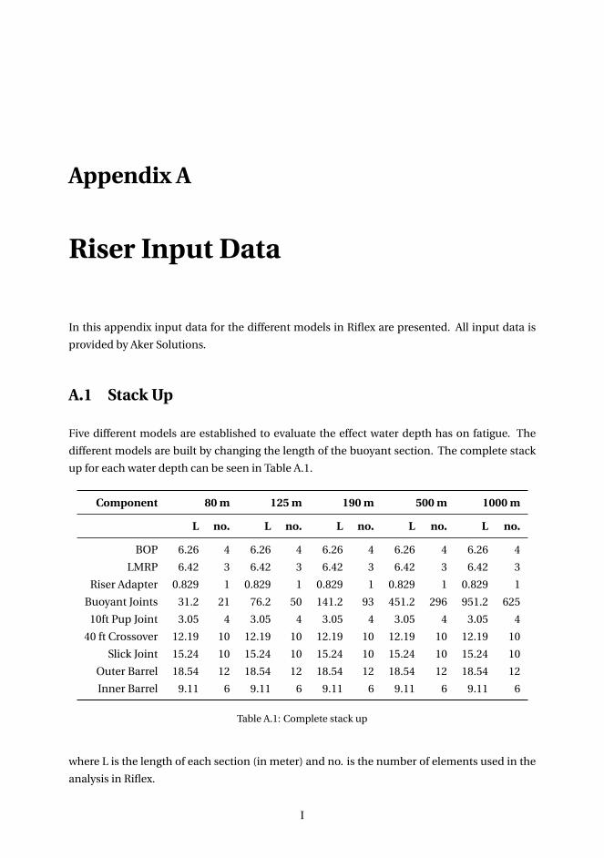
Appendix A
Riser Input Data
In this appendix input data for the different models in Riflex are presented. All input data is
provided by Aker Solutions.
A.1 Stack Up
Five different models are established to evaluate the effect water depth has on fatigue. The
different models are built by changing the length of the buoyant section. The complete stack
up for each water depth can be seen in Table A.1.
Component 80 m 125 m 190 m 500 m 1000 m
L no. L no. L no. L no. L no.
BOP 6.26 4 6.26 4 6.26 4 6.26 4 6.26 4
LMRP 6.42 3 6.42 3 6.42 3 6.42 3 6.42 3
Riser Adapter 0.829 1 0.829 1 0.829 1 0.829 1 0.829 1
Buoyant Joints 31.2 21 76.2 50 141.2 93 451.2 296 951.2 625
10ft Pup Joint 3.05 4 3.05 4 3.05 4 3.05 4 3.05 4
40 ft Crossover 12.19 10 12.19 10 12.19 10 12.19 10 12.19 10
Slick Joint 15.24 10 15.24 10 15.24 10 15.24 10 15.24 10
Outer Barrel 18.54 12 18.54 12 18.54 12 18.54 12 18.54 12
Inner Barrel 9.11 6 9.11 6 9.11 6 9.11 6 9.11 6
Table A.1: Complete stack up
where L is the length of each section (in meter) and no. is the number of elements used in the
analysis in Riflex.
I
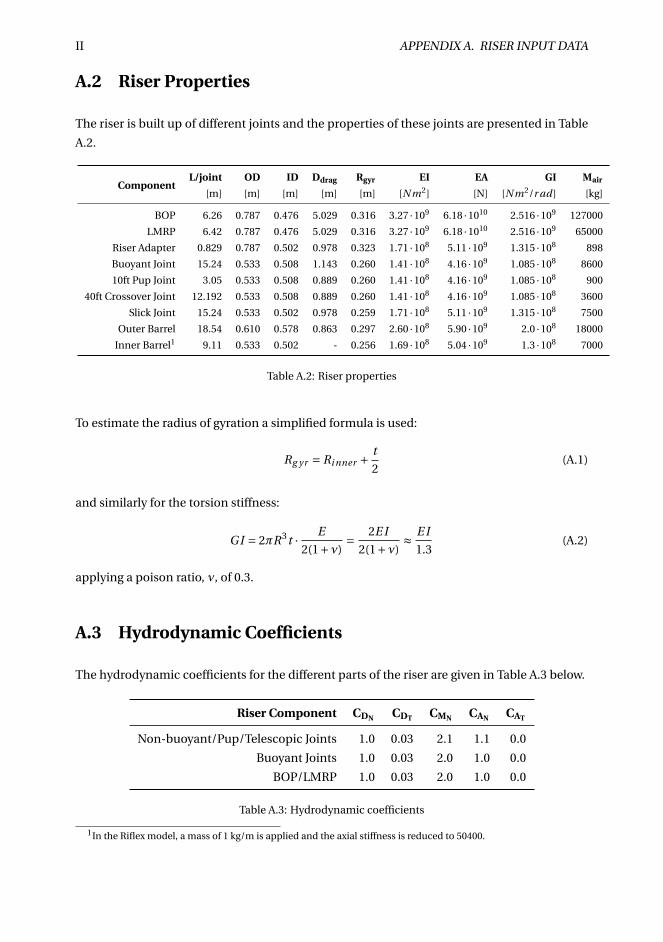
II APPENDIX A. RISER INPUT DATA
A.2 Riser Properties
The riser is built up of different joints and the properties of these joints are presented in Table
A.2.
ComponentL/joint OD ID Ddrag Rgyr EI EA GI Mair
[m] [m] [m] [m] [m] [N m2] [N] [N m2/r ad ] [kg]
BOP 6.26 0.787 0.476 5.029 0.316 3.27 ·109 6.18 ·1010 2.516 ·109 127000
LMRP 6.42 0.787 0.476 5.029 0.316 3.27 ·109 6.18 ·1010 2.516 ·109 65000
Riser Adapter 0.829 0.787 0.502 0.978 0.323 1.71 ·108 5.11 ·109 1.315 ·108 898
Buoyant Joint 15.24 0.533 0.508 1.143 0.260 1.41 ·108 4.16 ·109 1.085 ·108 8600
10ft Pup Joint 3.05 0.533 0.508 0.889 0.260 1.41 ·108 4.16 ·109 1.085 ·108 900
40ft Crossover Joint 12.192 0.533 0.508 0.889 0.260 1.41 ·108 4.16 ·109 1.085 ·108 3600
Slick Joint 15.24 0.533 0.502 0.978 0.259 1.71 ·108 5.11 ·109 1.315 ·108 7500
Outer Barrel 18.54 0.610 0.578 0.863 0.297 2.60 ·108 5.90 ·109 2.0 ·108 18000
Inner Barrel1 9.11 0.533 0.502 - 0.256 1.69 ·108 5.04 ·109 1.3 ·108 7000
Table A.2: Riser properties
To estimate the radius of gyration a simplified formula is used:
Rg yr = Ri nner + t
2(A.1)
and similarly for the torsion stiffness:
G I = 2πR3t · E
2(1+ν)= 2E I
2(1+ν)≈ E I
1.3(A.2)
applying a poison ratio, ν, of 0.3.
A.3 Hydrodynamic Coefficients
The hydrodynamic coefficients for the different parts of the riser are given in Table A.3 below.
Riser Component CDN CDT CMN CAN CAT
Non-buoyant/Pup/Telescopic Joints 1.0 0.03 2.1 1.1 0.0
Buoyant Joints 1.0 0.03 2.0 1.0 0.0
BOP/LMRP 1.0 0.03 2.0 1.0 0.0
Table A.3: Hydrodynamic coefficients
1In the Riflex model, a mass of 1 kg/m is applied and the axial stiffness is reduced to 50400.
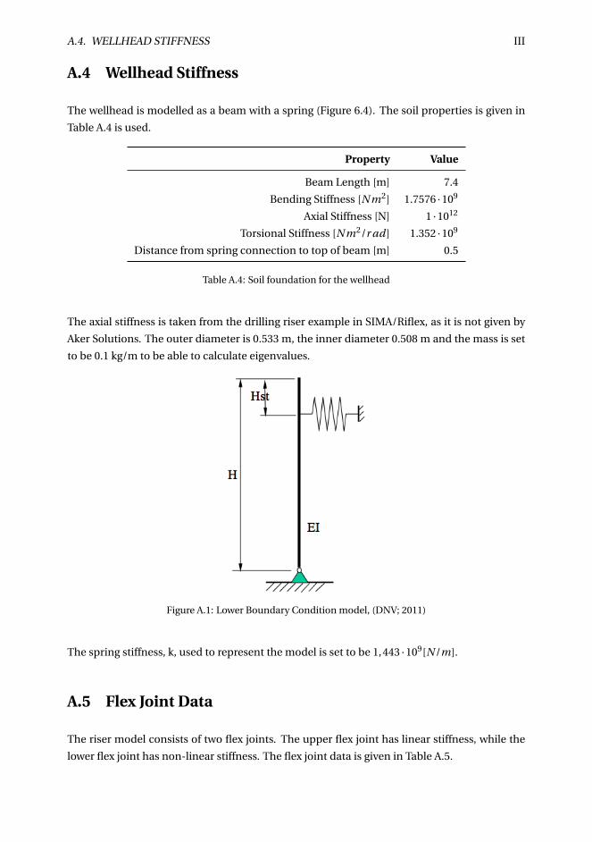
A.4. WELLHEAD STIFFNESS III
A.4 Wellhead Stiffness
The wellhead is modelled as a beam with a spring (Figure 6.4). The soil properties is given in
Table A.4 is used.
Property Value
Beam Length [m] 7.4
Bending Stiffness [N m2] 1.7576 ·109
Axial Stiffness [N] 1 ·1012
Torsional Stiffness [N m2/r ad ] 1.352 ·109
Distance from spring connection to top of beam [m] 0.5
Table A.4: Soil foundation for the wellhead
The axial stiffness is taken from the drilling riser example in SIMA/Riflex, as it is not given by
Aker Solutions. The outer diameter is 0.533 m, the inner diameter 0.508 m and the mass is set
to be 0.1 kg/m to be able to calculate eigenvalues.
Figure A.1: Lower Boundary Condition model, (DNV; 2011)
The spring stiffness, k, used to represent the model is set to be 1,443 ·109[N /m].
A.5 Flex Joint Data
The riser model consists of two flex joints. The upper flex joint has linear stiffness, while the
lower flex joint has non-linear stiffness. The flex joint data is given in Table A.5.
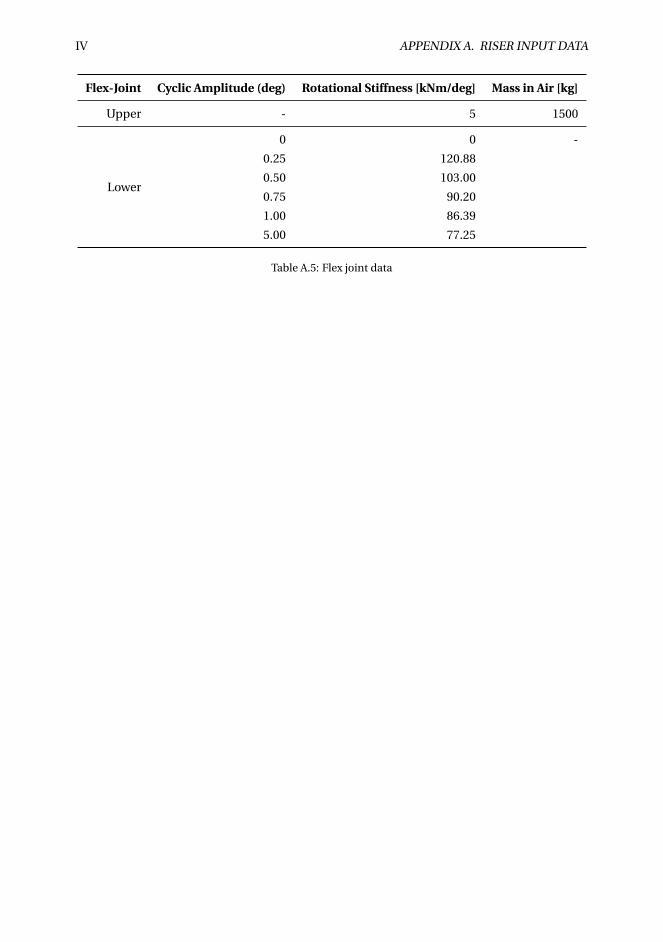
IV APPENDIX A. RISER INPUT DATA
Flex-Joint Cyclic Amplitude (deg) Rotational Stiffness [kNm/deg] Mass in Air [kg]
Upper - 5 1500
Lower
0 0 -
0.25 120.88
0.50 103.00
0.75 90.20
1.00 86.39
5.00 77.25
Table A.5: Flex joint data
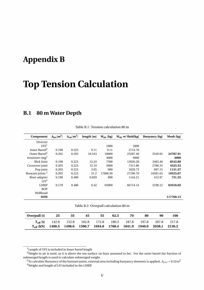
Appendix B
Top Tension Calculation
B.1 80 m Water Depth
Table B.1: Tension calculation 80 m
Component Aint[m2] Aext[m2] length [m] Mair [kg] Mair w/ fluid[kg] Buoyancy [kg] Msub [kg]
DiverterUFJ1 1800 1800
Inner Barrel2 0.198 0.223 9.11 9.11 2714.78Outer Barrel2 0.262 0.292 18.543 18000 25287.40 5549.92 24787.91
tensioner ring2 4000 4000 4000Slick Joint 0.198 0.223 15.24 7500 12026.28 3483.48 8542.80
Crossover joint 0.203 0.223 12.19 3600 7311.86 2786.33 4525.53Pup joint 0.203 0.223 3.05 900 1828.73 697.15 1131.57
Buoyant joints 3 0.203 0.223 31.2 17606.30 27106.70 16581.63 10525.07Riser adapter 0.198 0.486 0.829 898 1144.21 412.97 731.25
LFJ4
LMRP 0.178 0.486 6.42 65000 66714.14 3198.12 63516.02BOP
WellheadSUM 117760.13
Table B.2: Overpull calculation 80 m
Overpull [t] 25 35 45 55 62.5 70 80 90 100
Teff [t] 142.8 152.8 162.8 172.8 180.3 187.8 197.8 207.8 217.8Teff [kN] 1400.5 1498.6 1596.7 1694.8 1768.4 1841.9 1940.0 2038.1 2136.2
1Length of UFJ is included in Inner barrel length2Weight in air is used, as it is above the sea surface (at least assumed to be). For the outer barrel the fraction of
submerged length is used to calculate submerged weight.3To calculate Buoyancy of the buoyant joints, external area including buoyancy elements is applied, Aext = 0.52m2
4Weight and length of LFJ included in the LMRP.
V
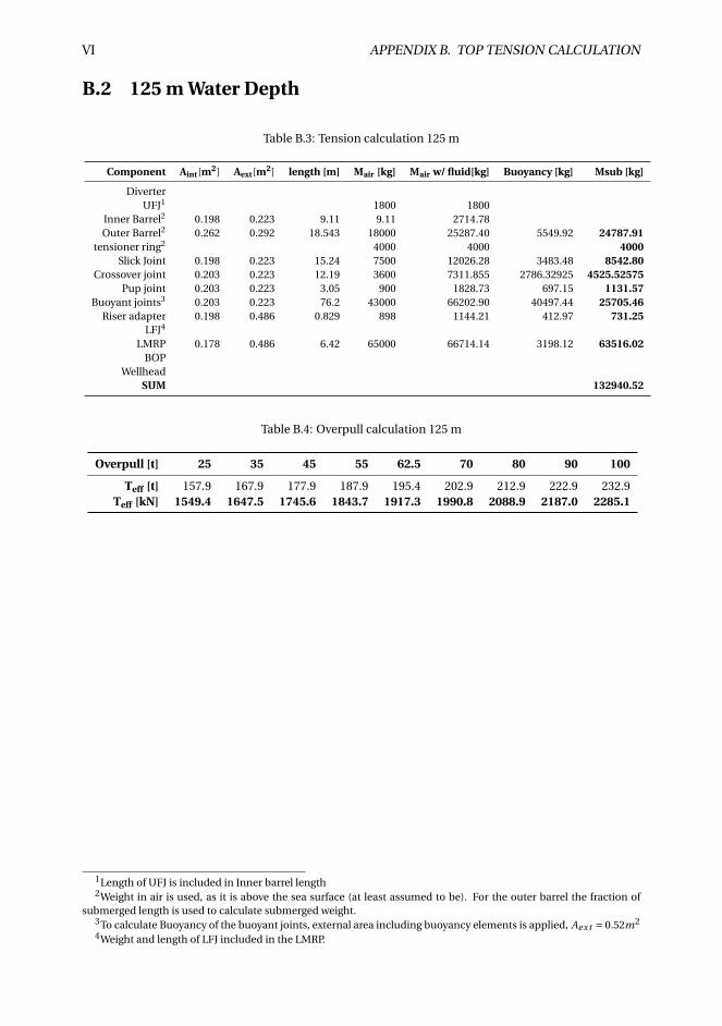
VI APPENDIX B. TOP TENSION CALCULATION
B.2 125 m Water Depth
Table B.3: Tension calculation 125 m
Component Aint[m2] Aext[m2] length [m] Mair [kg] Mair w/ fluid[kg] Buoyancy [kg] Msub [kg]
DiverterUFJ1 1800 1800
Inner Barrel2 0.198 0.223 9.11 9.11 2714.78Outer Barrel2 0.262 0.292 18.543 18000 25287.40 5549.92 24787.91
tensioner ring2 4000 4000 4000Slick Joint 0.198 0.223 15.24 7500 12026.28 3483.48 8542.80
Crossover joint 0.203 0.223 12.19 3600 7311.855 2786.32925 4525.52575Pup joint 0.203 0.223 3.05 900 1828.73 697.15 1131.57
Buoyant joints3 0.203 0.223 76.2 43000 66202.90 40497.44 25705.46Riser adapter 0.198 0.486 0.829 898 1144.21 412.97 731.25
LFJ4
LMRP 0.178 0.486 6.42 65000 66714.14 3198.12 63516.02BOP
WellheadSUM 132940.52
Table B.4: Overpull calculation 125 m
Overpull [t] 25 35 45 55 62.5 70 80 90 100
Teff [t] 157.9 167.9 177.9 187.9 195.4 202.9 212.9 222.9 232.9Teff [kN] 1549.4 1647.5 1745.6 1843.7 1917.3 1990.8 2088.9 2187.0 2285.1
1Length of UFJ is included in Inner barrel length2Weight in air is used, as it is above the sea surface (at least assumed to be). For the outer barrel the fraction of
submerged length is used to calculate submerged weight.3To calculate Buoyancy of the buoyant joints, external area including buoyancy elements is applied, Aext = 0.52m2
4Weight and length of LFJ included in the LMRP.
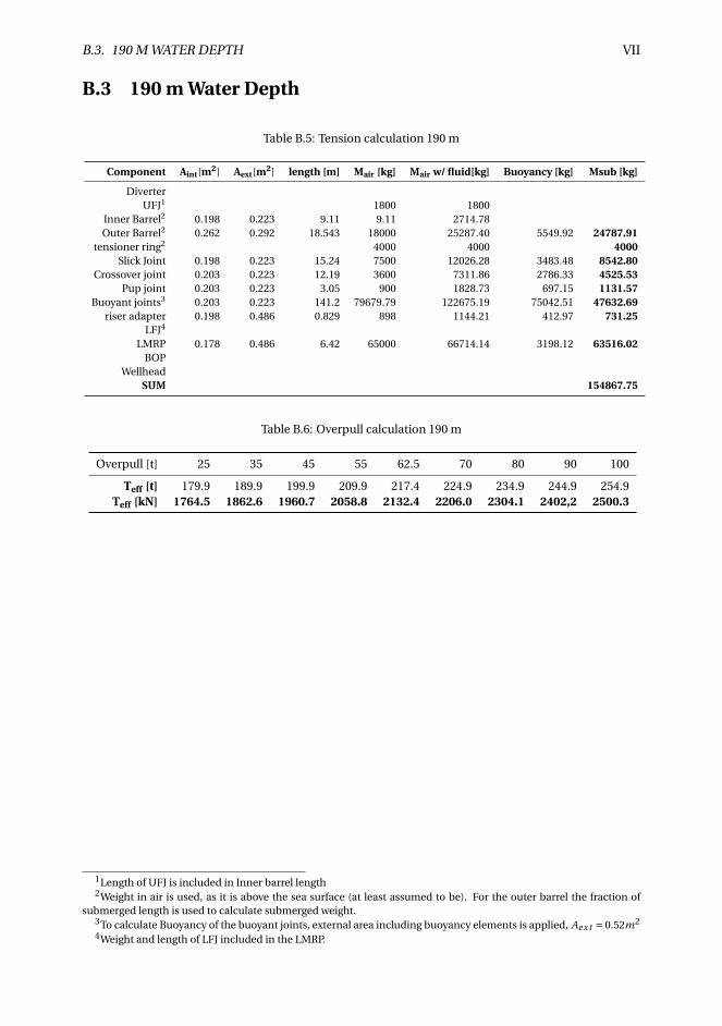
B.3. 190 M WATER DEPTH VII
B.3 190 m Water Depth
Table B.5: Tension calculation 190 m
Component Aint[m2] Aext[m2] length [m] Mair [kg] Mair w/ fluid[kg] Buoyancy [kg] Msub [kg]
DiverterUFJ1 1800 1800
Inner Barrel2 0.198 0.223 9.11 9.11 2714.78Outer Barrel2 0.262 0.292 18.543 18000 25287.40 5549.92 24787.91
tensioner ring2 4000 4000 4000Slick Joint 0.198 0.223 15.24 7500 12026.28 3483.48 8542.80
Crossover joint 0.203 0.223 12.19 3600 7311.86 2786.33 4525.53Pup joint 0.203 0.223 3.05 900 1828.73 697.15 1131.57
Buoyant joints3 0.203 0.223 141.2 79679.79 122675.19 75042.51 47632.69riser adapter 0.198 0.486 0.829 898 1144.21 412.97 731.25
LFJ4
LMRP 0.178 0.486 6.42 65000 66714.14 3198.12 63516.02BOP
WellheadSUM 154867.75
Table B.6: Overpull calculation 190 m
Overpull [t] 25 35 45 55 62.5 70 80 90 100
Teff [t] 179.9 189.9 199.9 209.9 217.4 224.9 234.9 244.9 254.9Teff [kN] 1764.5 1862.6 1960.7 2058.8 2132.4 2206.0 2304.1 2402,2 2500.3
1Length of UFJ is included in Inner barrel length2Weight in air is used, as it is above the sea surface (at least assumed to be). For the outer barrel the fraction of
submerged length is used to calculate submerged weight.3To calculate Buoyancy of the buoyant joints, external area including buoyancy elements is applied, Aext = 0.52m2
4Weight and length of LFJ included in the LMRP.
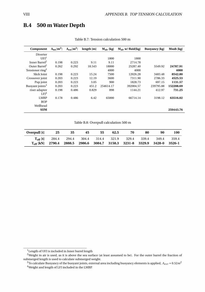
VIII APPENDIX B. TOP TENSION CALCULATION
B.4 500 m Water Depth
Table B.7: Tension calculation 500 m
Component Aint[m2] Aext[m2] length [m] Mair [kg] Mair w/ fluid[kg] Buoyancy [kg] Msub [kg]
DiverterUFJ1 1800 1800
Inner Barrel2 0.198 0.223 9.11 9.11 2714.78Outer Barrel2 0.262 0.292 18.543 18000 25287.40 5549.92 24787.91
Tensioner ring2 4000 4000 4000Slick Joint 0.198 0.223 15.24 7500 12026.28 3483.48 8542.80
Crossover joint 0.203 0.223 12.19 3600 7311.90 2786.33 4525.53Pup joint 0.203 0.223 3.05 900 1828.73 697.15 1131.57
Buoyant joints3 0.203 0.223 451.2 254614.17 392004.57 239795.88 152208.69riser adapter 0.198 0.486 0.829 898 1144.21 412.97 731.25
LFJ4
LMRP 0.178 0.486 6.42 65000 66714.14 3198.12 63516.02BOP
WellheadSUM 259443.76
Table B.8: Overpull calculation 500 m
Overpull [t] 25 35 45 55 62.5 70 80 90 100
Teff [t] 284.4 294.4 304.4 314.4 321.9 329.4 339.4 349.4 359.4Teff [kN] 2790.4 2888.5 2986.6 3084.7 3158.3 3231-8 3329.9 3428-0 3526-1
1Length of UFJ is included in Inner barrel length2Weight in air is used, as it is above the sea surface (at least assumed to be). For the outer barrel the fraction of
submerged length is used to calculate submerged weight.3To calculate Buoyancy of the buoyant joints, external area including buoyancy elements is applied, Aext = 0.52m2
4Weight and length of LFJ included in the LMRP.
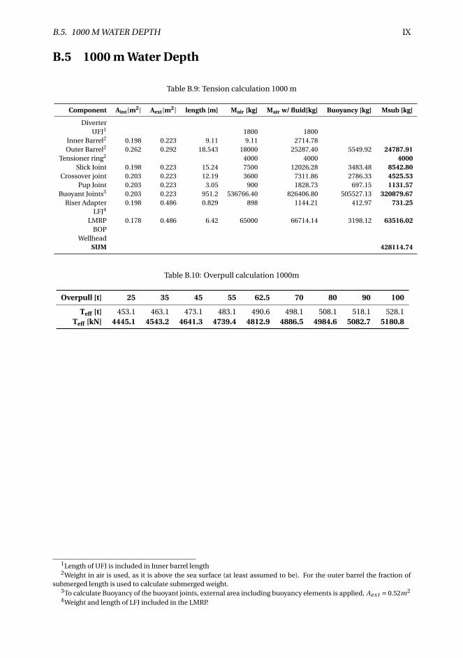
B.5. 1000 M WATER DEPTH IX
B.5 1000 m Water Depth
Table B.9: Tension calculation 1000 m
Component Aint[m2] Aext[m2] length [m] Mair [kg] Mair w/ fluid[kg] Buoyancy [kg] Msub [kg]
DiverterUFJ1 1800 1800
Inner Barrel2 0.198 0.223 9.11 9.11 2714.78Outer Barrel2 0.262 0.292 18.543 18000 25287.40 5549.92 24787.91
Tensioner ring2 4000 4000 4000Slick Joint 0.198 0.223 15.24 7500 12026.28 3483.48 8542.80
Crossover joint 0.203 0.223 12.19 3600 7311.86 2786.33 4525.53Pup Joint 0.203 0.223 3.05 900 1828.73 697.15 1131.57
Buoyant Joints3 0.203 0.223 951.2 536766.40 826406.80 505527.13 320879.67Riser Adapter 0.198 0.486 0.829 898 1144.21 412.97 731.25
LFJ4
LMRP 0.178 0.486 6.42 65000 66714.14 3198.12 63516.02BOP
WellheadSUM 428114.74
Table B.10: Overpull calculation 1000m
Overpull [t] 25 35 45 55 62.5 70 80 90 100
Teff [t] 453.1 463.1 473.1 483.1 490.6 498.1 508.1 518.1 528.1Teff [kN] 4445.1 4543.2 4641.3 4739.4 4812.9 4886.5 4984.6 5082.7 5180.8
1Length of UFJ is included in Inner barrel length2Weight in air is used, as it is above the sea surface (at least assumed to be). For the outer barrel the fraction of
submerged length is used to calculate submerged weight.3To calculate Buoyancy of the buoyant joints, external area including buoyancy elements is applied, Aext = 0.52m2
4Weight and length of LFJ included in the LMRP.

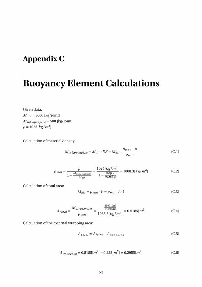
Appendix C
Buoyancy Element Calculations
Given data:
Mai r = 8600 [kg/joint]
Msub,openpi pe = 500 [kg/joint]
ρ = 1025[kg /m3]
Calculation of material density:
Msub,openpi pe = Mai r ·BF = Mai r · ρmat −ρρmat
(C.1)
ρmat = ρ
1− Msub,openpi pe
Mai r
= 1025[kg /m3]
1− 500[kg ]8600[kg ]
= 1088.3[kg /m3] (C.2)
Calculation of total area:
Mai r = ρmat ·V = ρmat · A ·1 (C.3)
ATot al =Mai r pr.meter
ρmat=
8600[kg ]15.24[m]
1088.3[kg /m3]= 0.5185[m2] (C.4)
Calculation of the external wrapping area:
ATot al = A Joi nt + Awr appi ng (C.5)
Awr appi ng = 0.5185[m2]−0.223[m2] = 0.2955[m2] (C.6)
XI

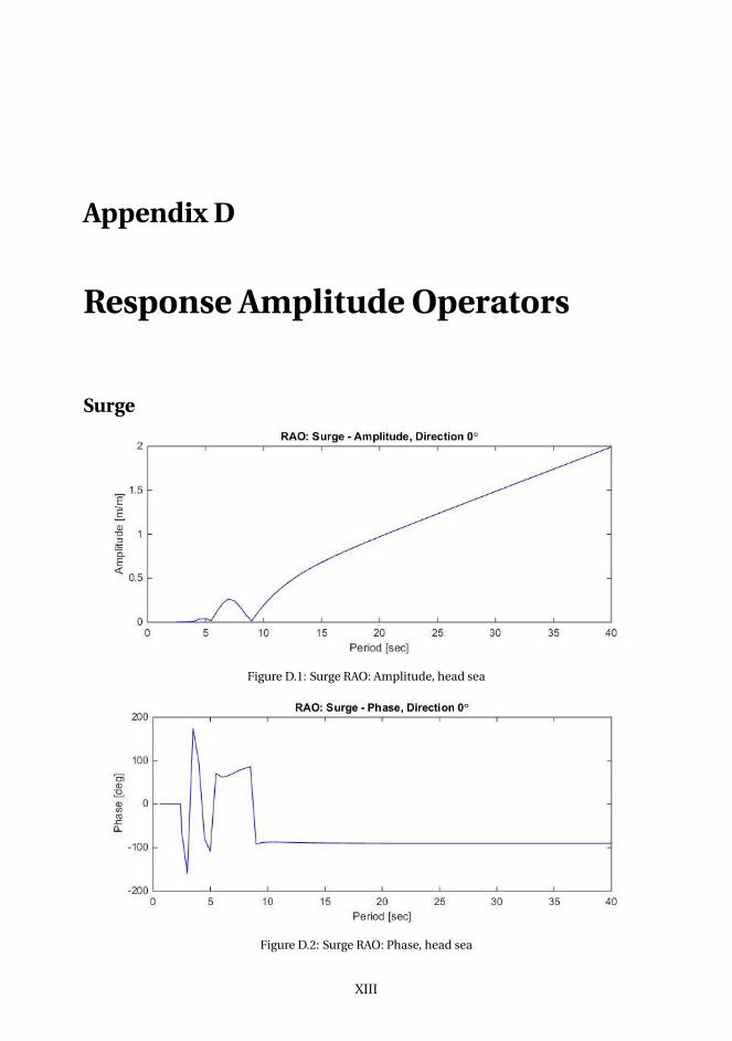
Appendix D
Response Amplitude Operators
Surge
Figure D.1: Surge RAO: Amplitude, head sea
Figure D.2: Surge RAO: Phase, head sea
XIII
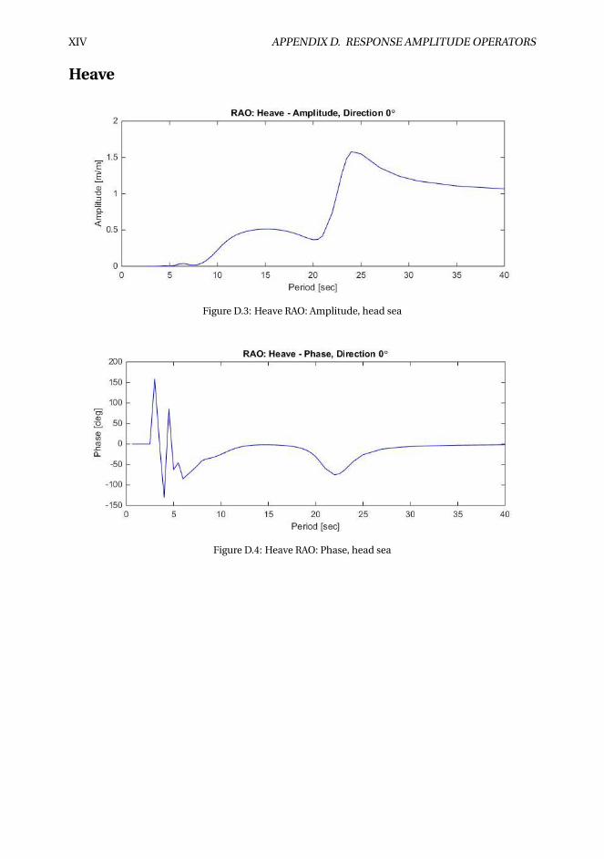
XIV APPENDIX D. RESPONSE AMPLITUDE OPERATORS
Heave
Figure D.3: Heave RAO: Amplitude, head sea
Figure D.4: Heave RAO: Phase, head sea
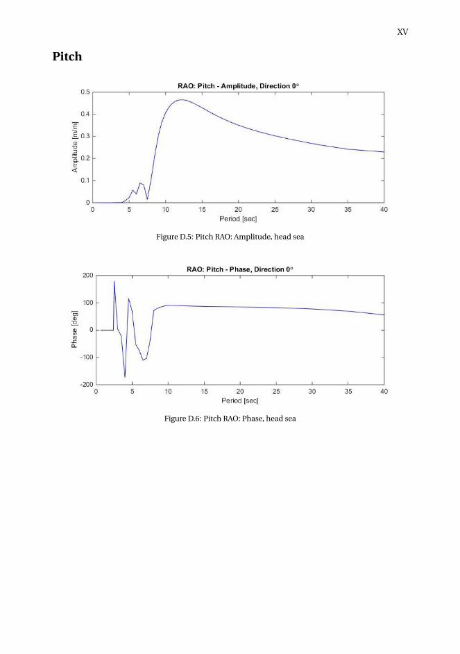
XV
Pitch
Figure D.5: Pitch RAO: Amplitude, head sea
Figure D.6: Pitch RAO: Phase, head sea

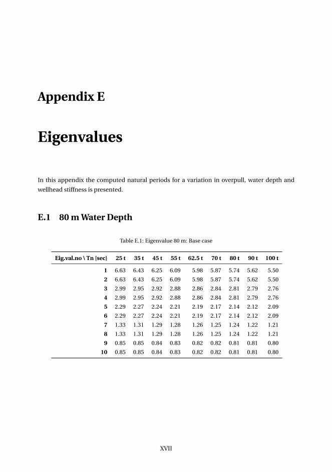
Appendix E
Eigenvalues
In this appendix the computed natural periods for a variation in overpull, water depth and
wellhead stiffness is presented.
E.1 80 m Water Depth
Table E.1: Eigenvalue 80 m: Base case
Eig.val.no \ Tn [sec] 25 t 35 t 45 t 55 t 62.5 t 70 t 80 t 90 t 100 t
1 6.63 6.43 6.25 6.09 5.98 5.87 5.74 5.62 5.50
2 6.63 6.43 6.25 6.09 5.98 5.87 5.74 5.62 5.50
3 2.99 2.95 2.92 2.88 2.86 2.84 2.81 2.79 2.76
4 2.99 2.95 2.92 2.88 2.86 2.84 2.81 2.79 2.76
5 2.29 2.27 2.24 2.21 2.19 2.17 2.14 2.12 2.09
6 2.29 2.27 2.24 2.21 2.19 2.17 2.14 2.12 2.09
7 1.33 1.31 1.29 1.28 1.26 1.25 1.24 1.22 1.21
8 1.33 1.31 1.29 1.28 1.26 1.25 1.24 1.22 1.21
9 0.85 0.85 0.84 0.83 0.82 0.82 0.81 0.81 0.80
10 0.85 0.85 0.84 0.83 0.82 0.82 0.81 0.81 0.80
XVII
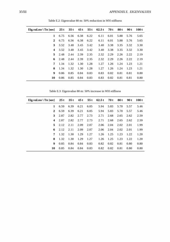
XVIII APPENDIX E. EIGENVALUES
Table E.2: Eigenvalue 80 m: 50% reduction in WH stiffness
Eig.val.no \ Tn [sec] 25 t 35 t 45 t 55 t 62.5 t 70 t 80 t 90 t 100 t
1 6.75 6.56 6.38 6.22 6.11 6.01 5.88 5.76 5.65
2 6.75 6.56 6.38 6.22 6.11 6.01 5.88 5.76 5.65
3 3.52 3.48 3.45 3.42 3.40 3.38 3.35 3.32 3.30
4 3.52 3.48 3.45 3.42 3.40 3.38 3.35 3.32 3.30
5 2.48 2.44 2.39 2.35 2.32 2.29 2.26 2.22 2.19
6 2.48 2.44 2.39 2.35 2.32 2.29 2.26 2.22 2.19
7 1.34 1.32 1.30 1.28 1.27 1.26 1.24 1.23 1.21
8 1.34 1.32 1.30 1.28 1.27 1.26 1.24 1.23 1.21
9 0.86 0.85 0.84 0.83 0.83 0.82 0.81 0.81 0.80
10 0.86 0.85 0.84 0.83 0.83 0.82 0.81 0.81 0.80
Table E.3: Eigenvalue 80 m: 50% increase in WH stiffness
Eig.val.no \ Tn [sec] 25 t 35 t 45 t 55 t 62.5 t 70 t 80 t 90 t 100 t
1 6.59 6.39 6.21 6.05 5.94 5.83 5.70 5.57 5.46
2 6.59 6.39 6.21 6.05 5.94 5.83 5.70 5.57 5.46
3 2.87 2.82 2.77 2.73 2.71 2.68 2.65 2.62 2.59
4 2.87 2.82 2.77 2.73 2.71 2.68 2.65 2.62 2.59
5 2.12 2.11 2.09 2.07 2.06 2.04 2.02 2.01 1.99
6 2.12 2.11 2.09 2.07 2.06 2.04 2.02 2.01 1.99
7 1.32 1.30 1.29 1.27 1.26 1.25 1.23 1.22 1.20
8 1.32 1.30 1.29 1.27 1.26 1.25 1.23 1.22 1.20
9 0.85 0.84 0.84 0.83 0.82 0.82 0.81 0.80 0.80
10 0.85 0.84 0.84 0.83 0.82 0.82 0.81 0.80 0.80
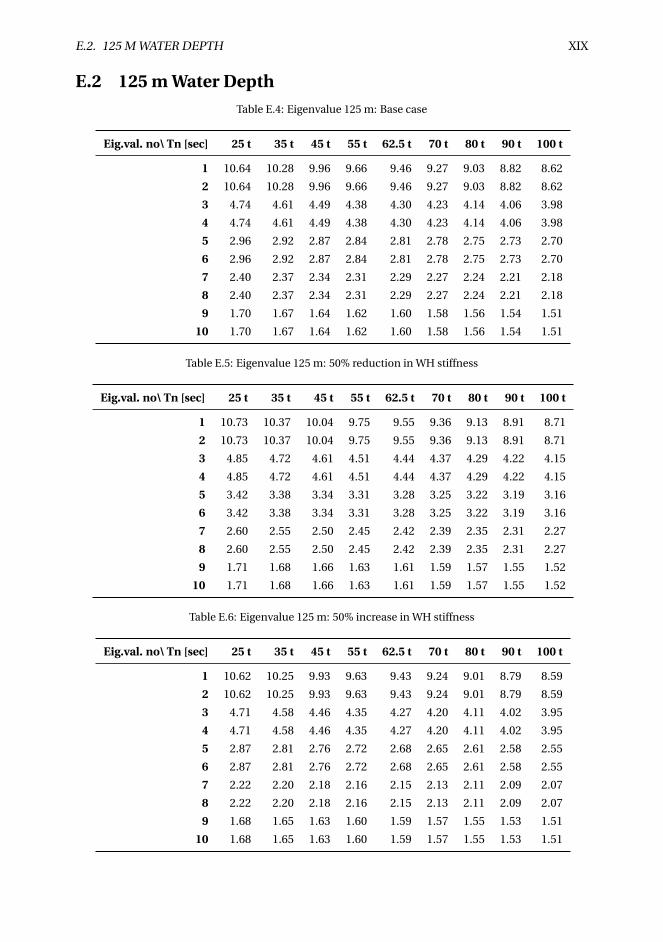
E.2. 125 M WATER DEPTH XIX
E.2 125 m Water Depth
Table E.4: Eigenvalue 125 m: Base case
Eig.val. no\ Tn [sec] 25 t 35 t 45 t 55 t 62.5 t 70 t 80 t 90 t 100 t
1 10.64 10.28 9.96 9.66 9.46 9.27 9.03 8.82 8.62
2 10.64 10.28 9.96 9.66 9.46 9.27 9.03 8.82 8.62
3 4.74 4.61 4.49 4.38 4.30 4.23 4.14 4.06 3.98
4 4.74 4.61 4.49 4.38 4.30 4.23 4.14 4.06 3.98
5 2.96 2.92 2.87 2.84 2.81 2.78 2.75 2.73 2.70
6 2.96 2.92 2.87 2.84 2.81 2.78 2.75 2.73 2.70
7 2.40 2.37 2.34 2.31 2.29 2.27 2.24 2.21 2.18
8 2.40 2.37 2.34 2.31 2.29 2.27 2.24 2.21 2.18
9 1.70 1.67 1.64 1.62 1.60 1.58 1.56 1.54 1.51
10 1.70 1.67 1.64 1.62 1.60 1.58 1.56 1.54 1.51
Table E.5: Eigenvalue 125 m: 50% reduction in WH stiffness
Eig.val. no\ Tn [sec] 25 t 35 t 45 t 55 t 62.5 t 70 t 80 t 90 t 100 t
1 10.73 10.37 10.04 9.75 9.55 9.36 9.13 8.91 8.71
2 10.73 10.37 10.04 9.75 9.55 9.36 9.13 8.91 8.71
3 4.85 4.72 4.61 4.51 4.44 4.37 4.29 4.22 4.15
4 4.85 4.72 4.61 4.51 4.44 4.37 4.29 4.22 4.15
5 3.42 3.38 3.34 3.31 3.28 3.25 3.22 3.19 3.16
6 3.42 3.38 3.34 3.31 3.28 3.25 3.22 3.19 3.16
7 2.60 2.55 2.50 2.45 2.42 2.39 2.35 2.31 2.27
8 2.60 2.55 2.50 2.45 2.42 2.39 2.35 2.31 2.27
9 1.71 1.68 1.66 1.63 1.61 1.59 1.57 1.55 1.52
10 1.71 1.68 1.66 1.63 1.61 1.59 1.57 1.55 1.52
Table E.6: Eigenvalue 125 m: 50% increase in WH stiffness
Eig.val. no\ Tn [sec] 25 t 35 t 45 t 55 t 62.5 t 70 t 80 t 90 t 100 t
1 10.62 10.25 9.93 9.63 9.43 9.24 9.01 8.79 8.59
2 10.62 10.25 9.93 9.63 9.43 9.24 9.01 8.79 8.59
3 4.71 4.58 4.46 4.35 4.27 4.20 4.11 4.02 3.95
4 4.71 4.58 4.46 4.35 4.27 4.20 4.11 4.02 3.95
5 2.87 2.81 2.76 2.72 2.68 2.65 2.61 2.58 2.55
6 2.87 2.81 2.76 2.72 2.68 2.65 2.61 2.58 2.55
7 2.22 2.20 2.18 2.16 2.15 2.13 2.11 2.09 2.07
8 2.22 2.20 2.18 2.16 2.15 2.13 2.11 2.09 2.07
9 1.68 1.65 1.63 1.60 1.59 1.57 1.55 1.53 1.51
10 1.68 1.65 1.63 1.60 1.59 1.57 1.55 1.53 1.51
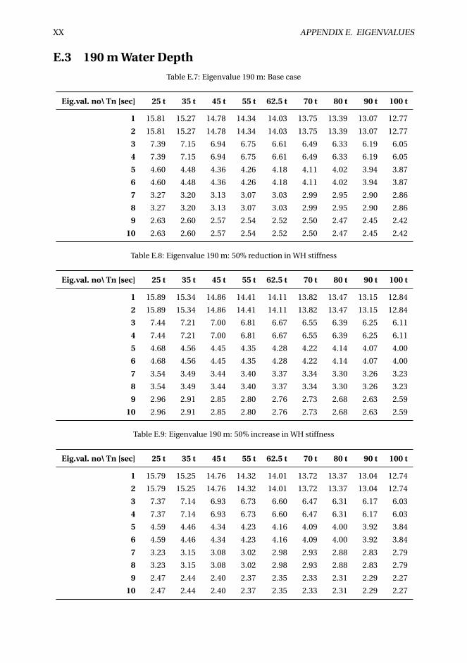
XX APPENDIX E. EIGENVALUES
E.3 190 m Water Depth
Table E.7: Eigenvalue 190 m: Base case
Eig.val. no\ Tn [sec] 25 t 35 t 45 t 55 t 62.5 t 70 t 80 t 90 t 100 t
1 15.81 15.27 14.78 14.34 14.03 13.75 13.39 13.07 12.77
2 15.81 15.27 14.78 14.34 14.03 13.75 13.39 13.07 12.77
3 7.39 7.15 6.94 6.75 6.61 6.49 6.33 6.19 6.05
4 7.39 7.15 6.94 6.75 6.61 6.49 6.33 6.19 6.05
5 4.60 4.48 4.36 4.26 4.18 4.11 4.02 3.94 3.87
6 4.60 4.48 4.36 4.26 4.18 4.11 4.02 3.94 3.87
7 3.27 3.20 3.13 3.07 3.03 2.99 2.95 2.90 2.86
8 3.27 3.20 3.13 3.07 3.03 2.99 2.95 2.90 2.86
9 2.63 2.60 2.57 2.54 2.52 2.50 2.47 2.45 2.42
10 2.63 2.60 2.57 2.54 2.52 2.50 2.47 2.45 2.42
Table E.8: Eigenvalue 190 m: 50% reduction in WH stiffness
Eig.val. no\ Tn [sec] 25 t 35 t 45 t 55 t 62.5 t 70 t 80 t 90 t 100 t
1 15.89 15.34 14.86 14.41 14.11 13.82 13.47 13.15 12.84
2 15.89 15.34 14.86 14.41 14.11 13.82 13.47 13.15 12.84
3 7.44 7.21 7.00 6.81 6.67 6.55 6.39 6.25 6.11
4 7.44 7.21 7.00 6.81 6.67 6.55 6.39 6.25 6.11
5 4.68 4.56 4.45 4.35 4.28 4.22 4.14 4.07 4.00
6 4.68 4.56 4.45 4.35 4.28 4.22 4.14 4.07 4.00
7 3.54 3.49 3.44 3.40 3.37 3.34 3.30 3.26 3.23
8 3.54 3.49 3.44 3.40 3.37 3.34 3.30 3.26 3.23
9 2.96 2.91 2.85 2.80 2.76 2.73 2.68 2.63 2.59
10 2.96 2.91 2.85 2.80 2.76 2.73 2.68 2.63 2.59
Table E.9: Eigenvalue 190 m: 50% increase in WH stiffness
Eig.val. no\ Tn [sec] 25 t 35 t 45 t 55 t 62.5 t 70 t 80 t 90 t 100 t
1 15.79 15.25 14.76 14.32 14.01 13.72 13.37 13.04 12.74
2 15.79 15.25 14.76 14.32 14.01 13.72 13.37 13.04 12.74
3 7.37 7.14 6.93 6.73 6.60 6.47 6.31 6.17 6.03
4 7.37 7.14 6.93 6.73 6.60 6.47 6.31 6.17 6.03
5 4.59 4.46 4.34 4.23 4.16 4.09 4.00 3.92 3.84
6 4.59 4.46 4.34 4.23 4.16 4.09 4.00 3.92 3.84
7 3.23 3.15 3.08 3.02 2.98 2.93 2.88 2.83 2.79
8 3.23 3.15 3.08 3.02 2.98 2.93 2.88 2.83 2.79
9 2.47 2.44 2.40 2.37 2.35 2.33 2.31 2.29 2.27
10 2.47 2.44 2.40 2.37 2.35 2.33 2.31 2.29 2.27
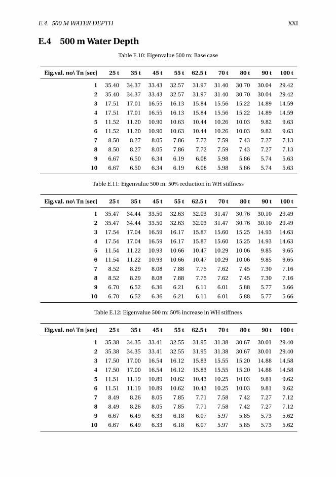
E.4. 500 M WATER DEPTH XXI
E.4 500 m Water Depth
Table E.10: Eigenvalue 500 m: Base case
Eig.val. no\ Tn [sec] 25 t 35 t 45 t 55 t 62.5 t 70 t 80 t 90 t 100 t
1 35.40 34.37 33.43 32.57 31.97 31.40 30.70 30.04 29.42
2 35.40 34.37 33.43 32.57 31.97 31.40 30.70 30.04 29.42
3 17.51 17.01 16.55 16.13 15.84 15.56 15.22 14.89 14.59
4 17.51 17.01 16.55 16.13 15.84 15.56 15.22 14.89 14.59
5 11.52 11.20 10.90 10.63 10.44 10.26 10.03 9.82 9.63
6 11.52 11.20 10.90 10.63 10.44 10.26 10.03 9.82 9.63
7 8.50 8.27 8.05 7.86 7.72 7.59 7.43 7.27 7.13
8 8.50 8.27 8.05 7.86 7.72 7.59 7.43 7.27 7.13
9 6.67 6.50 6.34 6.19 6.08 5.98 5.86 5.74 5.63
10 6.67 6.50 6.34 6.19 6.08 5.98 5.86 5.74 5.63
Table E.11: Eigenvalue 500 m: 50% reduction in WH stiffness
Eig.val. no\ Tn [sec] 25 t 35 t 45 t 55 t 62.5 t 70 t 80 t 90 t 100 t
1 35.47 34.44 33.50 32.63 32.03 31.47 30.76 30.10 29.49
2 35.47 34.44 33.50 32.63 32.03 31.47 30.76 30.10 29.49
3 17.54 17.04 16.59 16.17 15.87 15.60 15.25 14.93 14.63
4 17.54 17.04 16.59 16.17 15.87 15.60 15.25 14.93 14.63
5 11.54 11.22 10.93 10.66 10.47 10.29 10.06 9.85 9.65
6 11.54 11.22 10.93 10.66 10.47 10.29 10.06 9.85 9.65
7 8.52 8.29 8.08 7.88 7.75 7.62 7.45 7.30 7.16
8 8.52 8.29 8.08 7.88 7.75 7.62 7.45 7.30 7.16
9 6.70 6.52 6.36 6.21 6.11 6.01 5.88 5.77 5.66
10 6.70 6.52 6.36 6.21 6.11 6.01 5.88 5.77 5.66
Table E.12: Eigenvalue 500 m: 50% increase in WH stiffness
Eig.val. no\ Tn [sec] 25 t 35 t 45 t 55 t 62.5 t 70 t 80 t 90 t 100 t
1 35.38 34.35 33.41 32.55 31.95 31.38 30.67 30.01 29.40
2 35.38 34.35 33.41 32.55 31.95 31.38 30.67 30.01 29.40
3 17.50 17.00 16.54 16.12 15.83 15.55 15.20 14.88 14.58
4 17.50 17.00 16.54 16.12 15.83 15.55 15.20 14.88 14.58
5 11.51 11.19 10.89 10.62 10.43 10.25 10.03 9.81 9.62
6 11.51 11.19 10.89 10.62 10.43 10.25 10.03 9.81 9.62
7 8.49 8.26 8.05 7.85 7.71 7.58 7.42 7.27 7.12
8 8.49 8.26 8.05 7.85 7.71 7.58 7.42 7.27 7.12
9 6.67 6.49 6.33 6.18 6.07 5.97 5.85 5.73 5.62
10 6.67 6.49 6.33 6.18 6.07 5.97 5.85 5.73 5.62
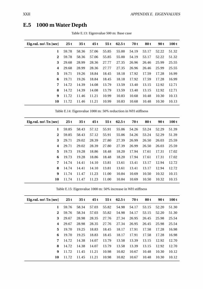
XXII APPENDIX E. EIGENVALUES
E.5 1000 m Water DepthTable E.13: Eigenvalue 500 m: Base case
Eig.val. no\ Tn [sec] 25 t 35 t 45 t 55 t 62.5 t 70 t 80 t 90 t 100 t
1 59.78 58.36 57.06 55.85 55.00 54.19 53.17 52.22 51.32
2 59.78 58.36 57.06 55.85 55.00 54.19 53.17 52.22 51.32
3 29.68 28.99 28.36 27.77 27.35 26.96 26.46 25.99 25.55
4 29.68 28.99 28.36 27.77 27.35 26.96 26.46 25.99 25.55
5 19.71 19.26 18.84 18.45 18.18 17.92 17.59 17.28 16.99
6 19.71 19.26 18.84 18.45 18.18 17.92 17.59 17.28 16.99
7 14.72 14.39 14.08 13.79 13.59 13.40 13.15 12.92 12.71
8 14.72 14.39 14.08 13.79 13.59 13.40 13.15 12.92 12.71
9 11.72 11.46 11.21 10.99 10.83 10.68 10.48 10.30 10.13
10 11.72 11.46 11.21 10.99 10.83 10.68 10.48 10.30 10.13
Table E.14: Eigenvalue 1000 m: 50% reduction in WH stiffness
Eig.val. no\ Tn [sec] 25 t 35 t 45 t 55 t 62.5 t 70 t 80 t 90 t 100 t
1 59.85 58.43 57.12 55.91 55.06 54.26 53.24 52.29 51.39
2 59.85 58.43 57.12 55.91 55.06 54.26 53.24 52.29 51.39
3 29.71 29.02 28.39 27.80 27.39 26.99 26.50 26.03 25.59
4 29.71 29.02 28.39 27.80 27.39 26.99 26.50 26.03 25.59
5 19.73 19.28 18.86 18.48 18.20 17.94 17.61 17.31 17.02
6 19.73 19.28 18.86 18.48 18.20 17.94 17.61 17.31 17.02
7 14.74 14.41 14.10 13.81 13.61 13.41 13.17 12.94 12.72
8 14.74 14.41 14.10 13.81 13.61 13.41 13.17 12.94 12.72
9 11.74 11.47 11.23 11.00 10.84 10.69 10.50 10.32 10.15
10 11.74 11.47 11.23 11.00 10.84 10.69 10.50 10.32 10.15
Table E.15: Eigenvalue 1000 m: 50% increase in WH stiffness
Eig.val. no\ Tn [sec] 25 t 35 t 45 t 55 t 62.5 t 70 t 80 t 90 t 100 t
1 59.76 58.34 57.03 55.82 54.98 54.17 53.15 52.20 51.30
2 59.76 58.34 57.03 55.82 54.98 54.17 53.15 52.20 51.30
3 29.67 28.98 28.35 27.76 27.34 26.95 26.45 25.98 25.54
4 29.67 28.98 28.35 27.76 27.34 26.95 26.45 25.98 25.54
5 19.70 19.25 18.83 18.45 18.17 17.91 17.58 17.28 16.98
6 19.70 19.25 18.83 18.45 18.17 17.91 17.58 17.28 16.98
7 14.72 14.38 14.07 13.79 13.58 13.39 13.15 12.92 12.70
8 14.72 14.38 14.07 13.79 13.58 13.39 13.15 12.92 12.70
9 11.72 11.45 11.21 10.98 10.82 10.67 10.48 10.30 10.12
10 11.72 11.45 11.21 10.98 10.82 10.67 10.48 10.30 10.12
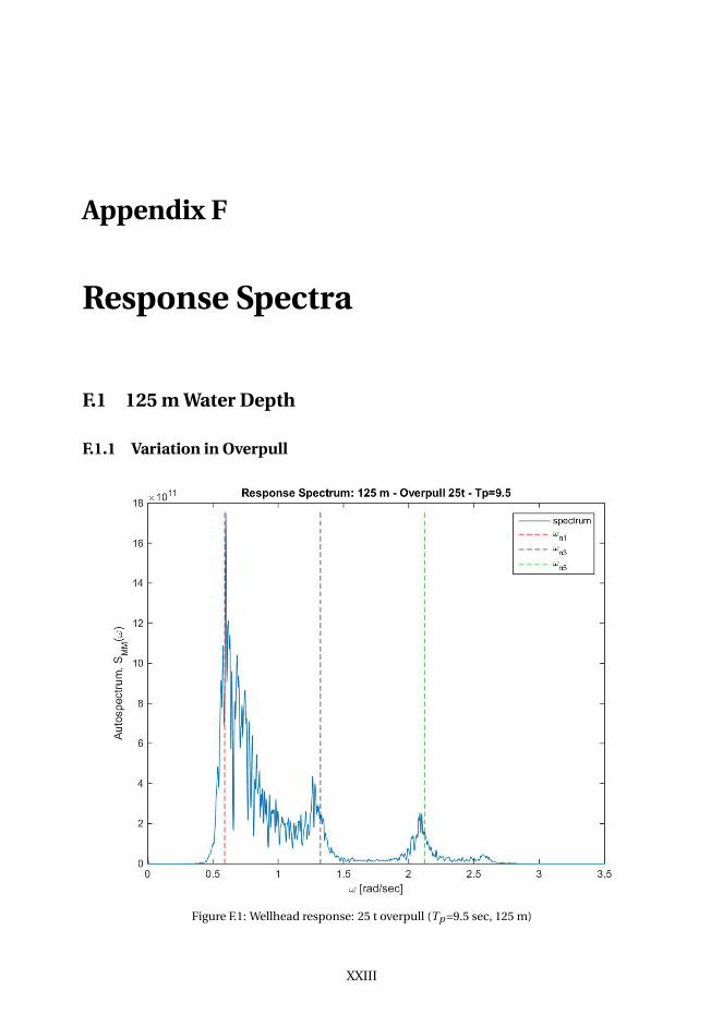
Appendix F
Response Spectra
F.1 125 m Water Depth
F.1.1 Variation in Overpull
Figure F.1: Wellhead response: 25 t overpull (Tp =9.5 sec, 125 m)
XXIII
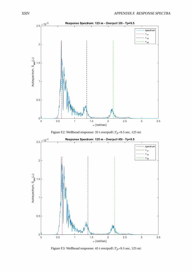
XXIV APPENDIX F. RESPONSE SPECTRA
Figure F.2: Wellhead response: 35 t overpull (Tp =9.5 sec, 125 m)
Figure F.3: Wellhead response: 45 t overpull (Tp =9.5 sec, 125 m)
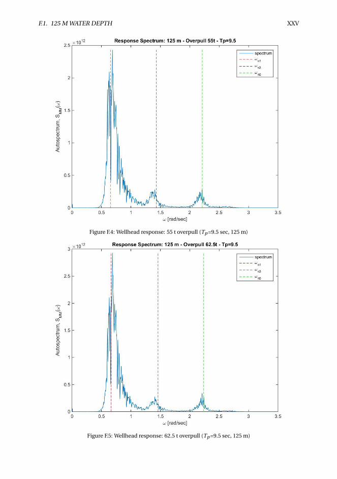
F.1. 125 M WATER DEPTH XXV
Figure F.4: Wellhead response: 55 t overpull (Tp =9.5 sec, 125 m)
Figure F.5: Wellhead response: 62.5 t overpull (Tp =9.5 sec, 125 m)
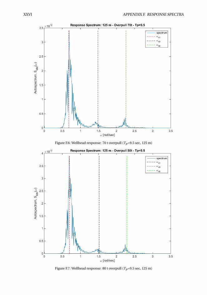
XXVI APPENDIX F. RESPONSE SPECTRA
Figure F.6: Wellhead response: 70 t overpull (Tp =9.5 sec, 125 m)
Figure F.7: Wellhead response: 80 t overpull (Tp =9.5 sec, 125 m)
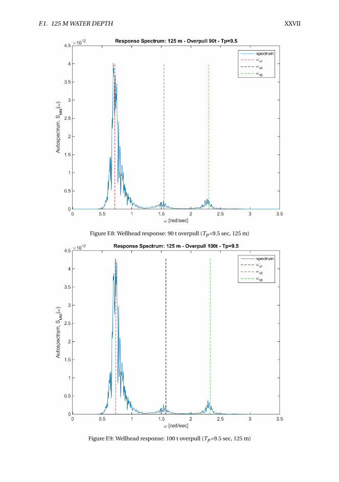
F.1. 125 M WATER DEPTH XXVII
Figure F.8: Wellhead response: 90 t overpull (Tp =9.5 sec, 125 m)
Figure F.9: Wellhead response: 100 t overpull (Tp =9.5 sec, 125 m)
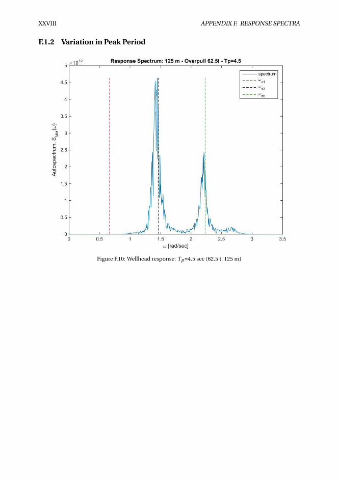
XXVIII APPENDIX F. RESPONSE SPECTRA
F.1.2 Variation in Peak Period
Figure F.10: Wellhead response: Tp =4.5 sec (62.5 t, 125 m)
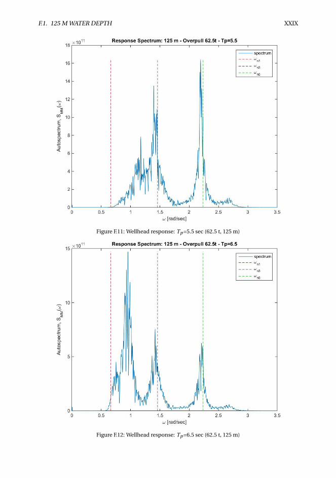
F.1. 125 M WATER DEPTH XXIX
Figure F.11: Wellhead response: Tp =5.5 sec (62.5 t, 125 m)
Figure F.12: Wellhead response: Tp =6.5 sec (62.5 t, 125 m)
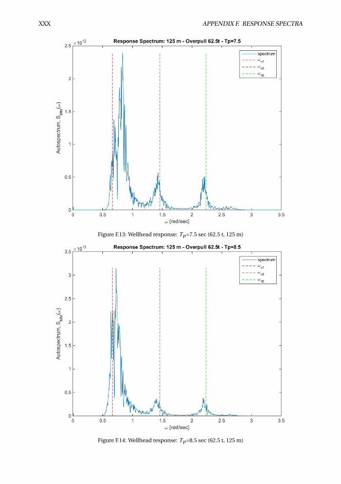
XXX APPENDIX F. RESPONSE SPECTRA
Figure F.13: Wellhead response: Tp =7.5 sec (62.5 t, 125 m)
Figure F.14: Wellhead response: Tp =8.5 sec (62.5 t, 125 m)
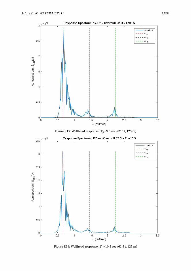
F.1. 125 M WATER DEPTH XXXI
Figure F.15: Wellhead response: Tp =9.5 sec (62.5 t, 125 m)
Figure F.16: Wellhead response: Tp =10.5 sec (62.5 t, 125 m)
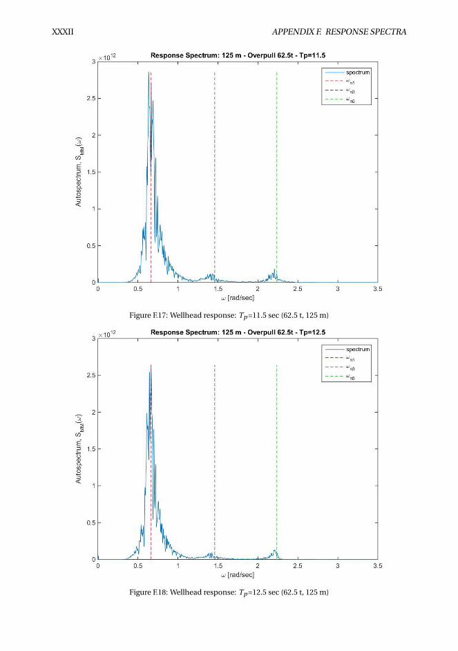
XXXII APPENDIX F. RESPONSE SPECTRA
Figure F.17: Wellhead response: Tp =11.5 sec (62.5 t, 125 m)
Figure F.18: Wellhead response: Tp =12.5 sec (62.5 t, 125 m)
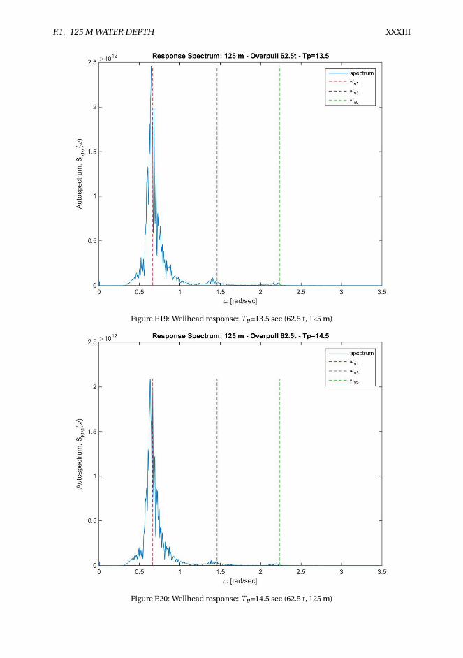
F.1. 125 M WATER DEPTH XXXIII
Figure F.19: Wellhead response: Tp =13.5 sec (62.5 t, 125 m)
Figure F.20: Wellhead response: Tp =14.5 sec (62.5 t, 125 m)

XXXIV APPENDIX F. RESPONSE SPECTRA
Figure F.21: Wellhead response: Tp =15.5 sec (62.5 t, 125 m)
Figure F.22: Wellhead response: Tp =16.5 sec (62.5 t, 125 m)

F.1. 125 M WATER DEPTH XXXV
Figure F.23: Wellhead response: Tp =17.5 sec (62.5 t, 125 m)
Figure F.24: Wellhead response: Tp =18.5 sec (62.5 t, 125 m)
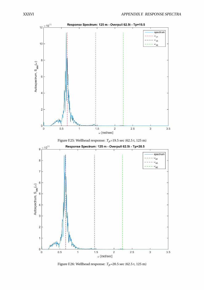
XXXVI APPENDIX F. RESPONSE SPECTRA
Figure F.25: Wellhead response: Tp =19.5 sec (62.5 t, 125 m)
Figure F.26: Wellhead response: Tp =20.5 sec (62.5 t, 125 m)
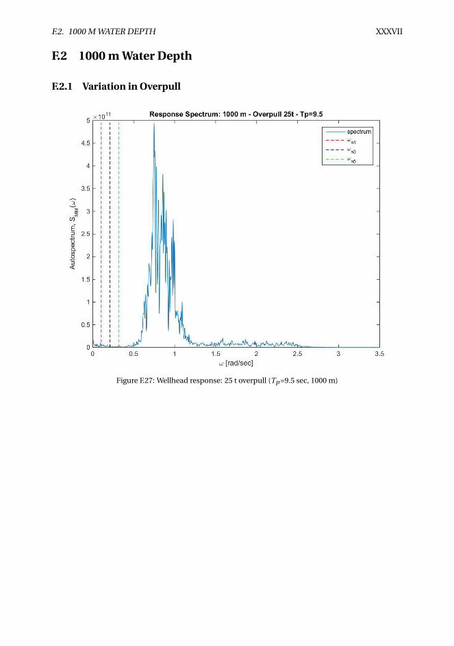
F.2. 1000 M WATER DEPTH XXXVII
F.2 1000 m Water Depth
F.2.1 Variation in Overpull
Figure F.27: Wellhead response: 25 t overpull (Tp =9.5 sec, 1000 m)
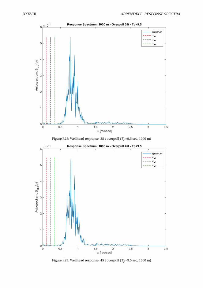
XXXVIII APPENDIX F. RESPONSE SPECTRA
Figure F.28: Wellhead response: 35 t overpull (Tp =9.5 sec, 1000 m)
Figure F.29: Wellhead response: 45 t overpull (Tp =9.5 sec, 1000 m)
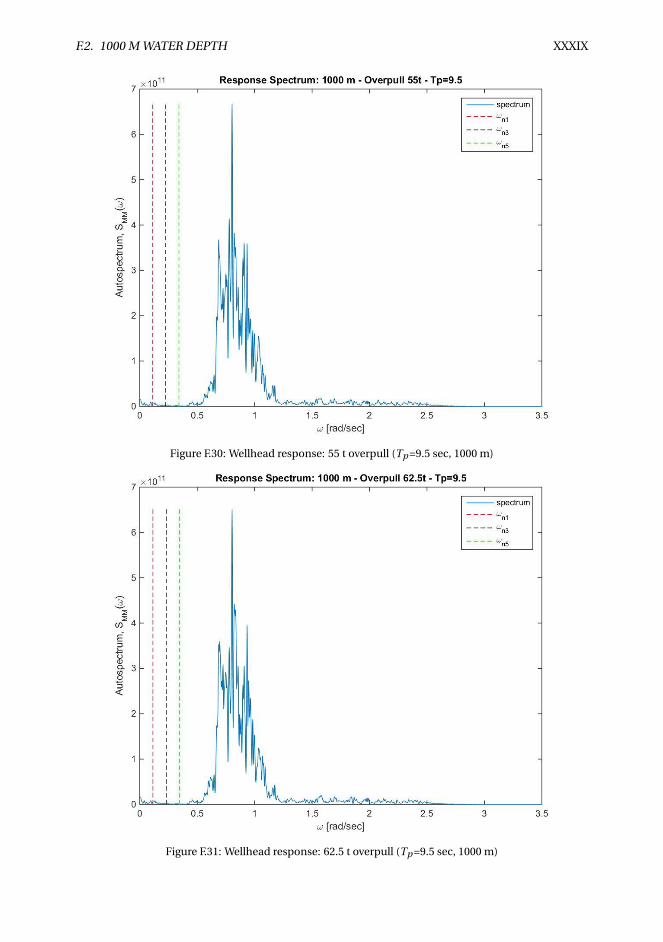
F.2. 1000 M WATER DEPTH XXXIX
Figure F.30: Wellhead response: 55 t overpull (Tp =9.5 sec, 1000 m)
Figure F.31: Wellhead response: 62.5 t overpull (Tp =9.5 sec, 1000 m)
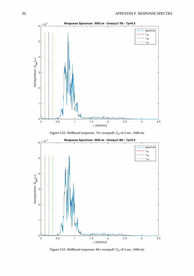
XL APPENDIX F. RESPONSE SPECTRA
Figure F.32: Wellhead response: 70 t overpull (Tp =9.5 sec, 1000 m)
Figure F.33: Wellhead response: 80 t overpull (Tp =9.5 sec, 1000 m)
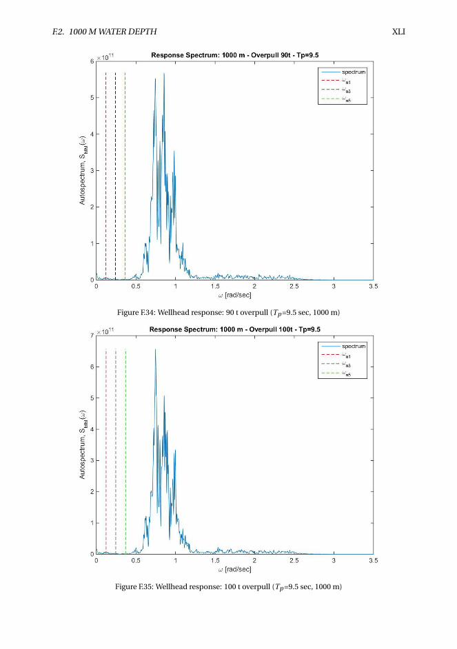
F.2. 1000 M WATER DEPTH XLI
Figure F.34: Wellhead response: 90 t overpull (Tp =9.5 sec, 1000 m)
Figure F.35: Wellhead response: 100 t overpull (Tp =9.5 sec, 1000 m)
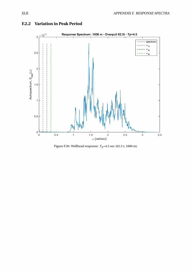
XLII APPENDIX F. RESPONSE SPECTRA
F.2.2 Variation in Peak Period
Figure F.36: Wellhead response: Tp =4.5 sec (62.5 t, 1000 m)
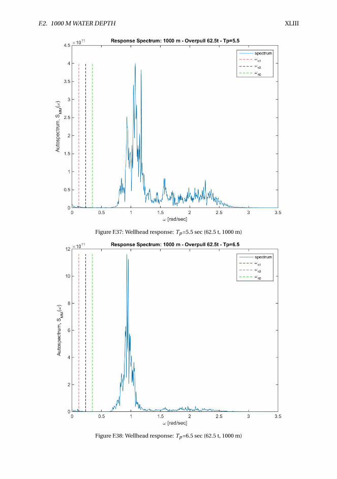
F.2. 1000 M WATER DEPTH XLIII
Figure F.37: Wellhead response: Tp =5.5 sec (62.5 t, 1000 m)
Figure F.38: Wellhead response: Tp =6.5 sec (62.5 t, 1000 m)
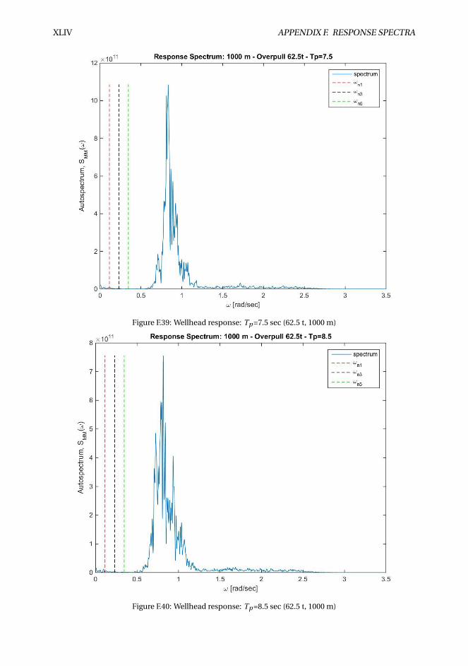
XLIV APPENDIX F. RESPONSE SPECTRA
Figure F.39: Wellhead response: Tp =7.5 sec (62.5 t, 1000 m)
Figure F.40: Wellhead response: Tp =8.5 sec (62.5 t, 1000 m)
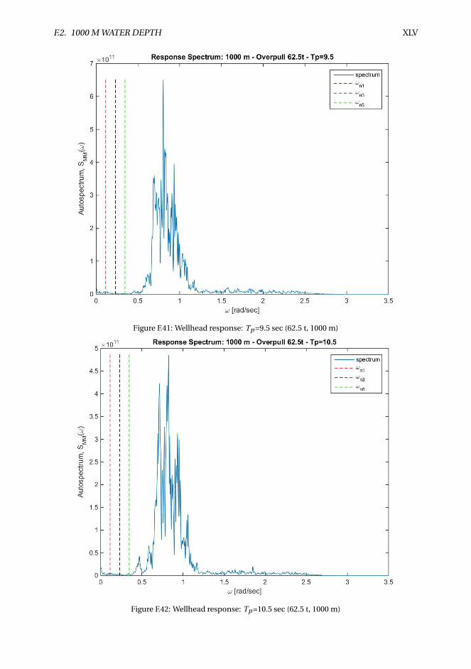
F.2. 1000 M WATER DEPTH XLV
Figure F.41: Wellhead response: Tp =9.5 sec (62.5 t, 1000 m)
Figure F.42: Wellhead response: Tp =10.5 sec (62.5 t, 1000 m)
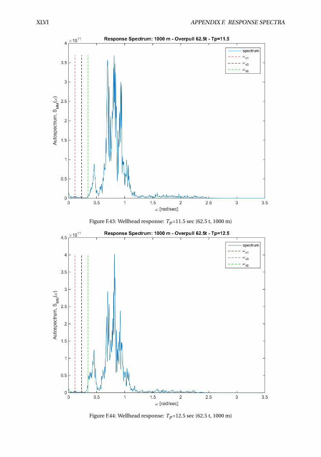
XLVI APPENDIX F. RESPONSE SPECTRA
Figure F.43: Wellhead response: Tp =11.5 sec (62.5 t, 1000 m)
Figure F.44: Wellhead response: Tp =12.5 sec (62.5 t, 1000 m)
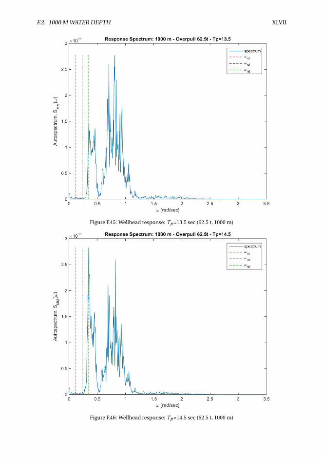
F.2. 1000 M WATER DEPTH XLVII
Figure F.45: Wellhead response: Tp =13.5 sec (62.5 t, 1000 m)
Figure F.46: Wellhead response: Tp =14.5 sec (62.5 t, 1000 m)
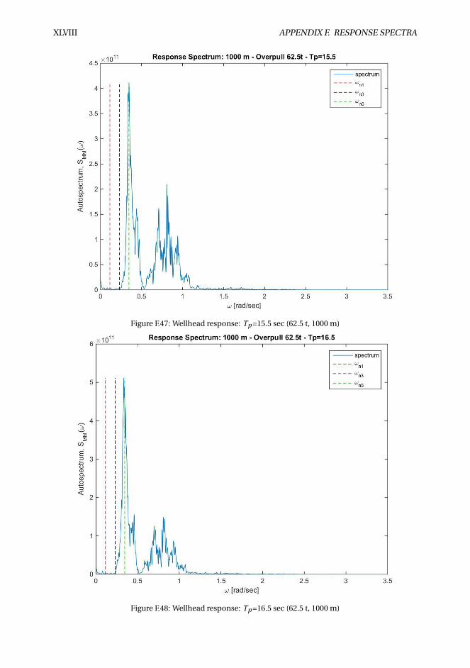
XLVIII APPENDIX F. RESPONSE SPECTRA
Figure F.47: Wellhead response: Tp =15.5 sec (62.5 t, 1000 m)
Figure F.48: Wellhead response: Tp =16.5 sec (62.5 t, 1000 m)
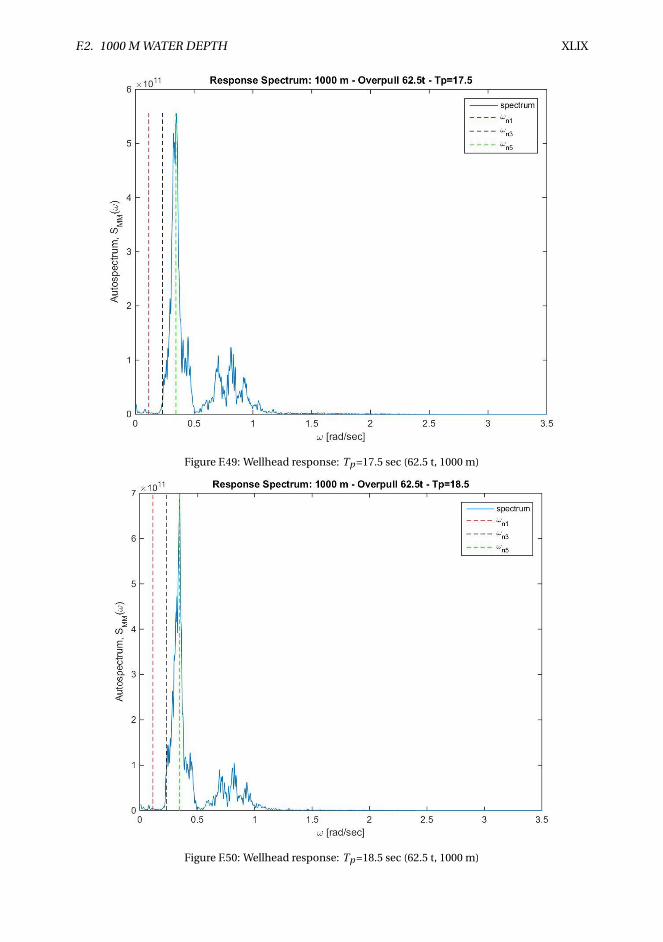
F.2. 1000 M WATER DEPTH XLIX
Figure F.49: Wellhead response: Tp =17.5 sec (62.5 t, 1000 m)
Figure F.50: Wellhead response: Tp =18.5 sec (62.5 t, 1000 m)
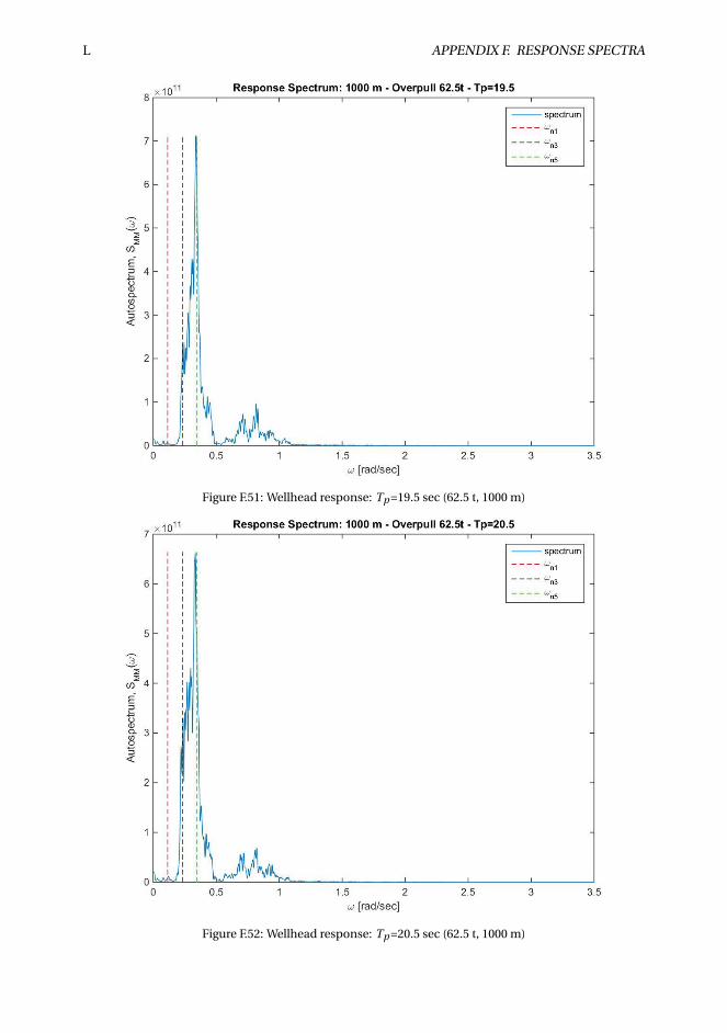
L APPENDIX F. RESPONSE SPECTRA
Figure F.51: Wellhead response: Tp =19.5 sec (62.5 t, 1000 m)
Figure F.52: Wellhead response: Tp =20.5 sec (62.5 t, 1000 m)
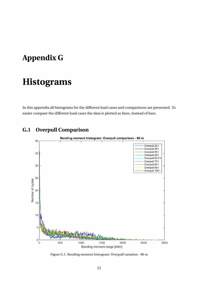
Appendix G
Histograms
In this appendix all histograms for the different load cases and comparisons are presented. To
easier compare the different load cases the data is plotted as lines, instead of bars.
G.1 Overpull Comparison
Figure G.1: Bending moment histogram: Overpull variation - 80 m
LI
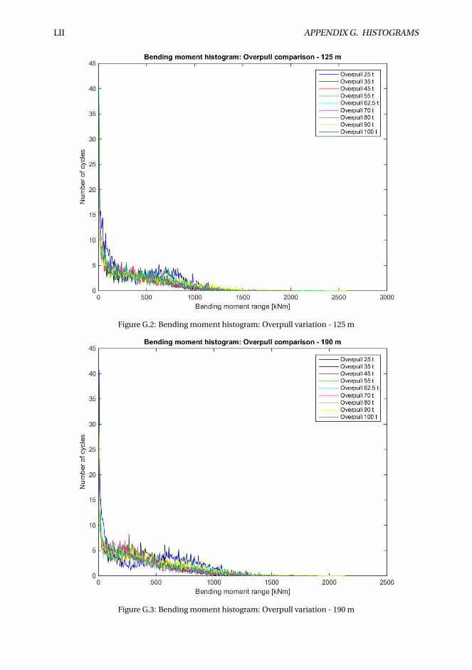
LII APPENDIX G. HISTOGRAMS
Figure G.2: Bending moment histogram: Overpull variation - 125 m
Figure G.3: Bending moment histogram: Overpull variation - 190 m
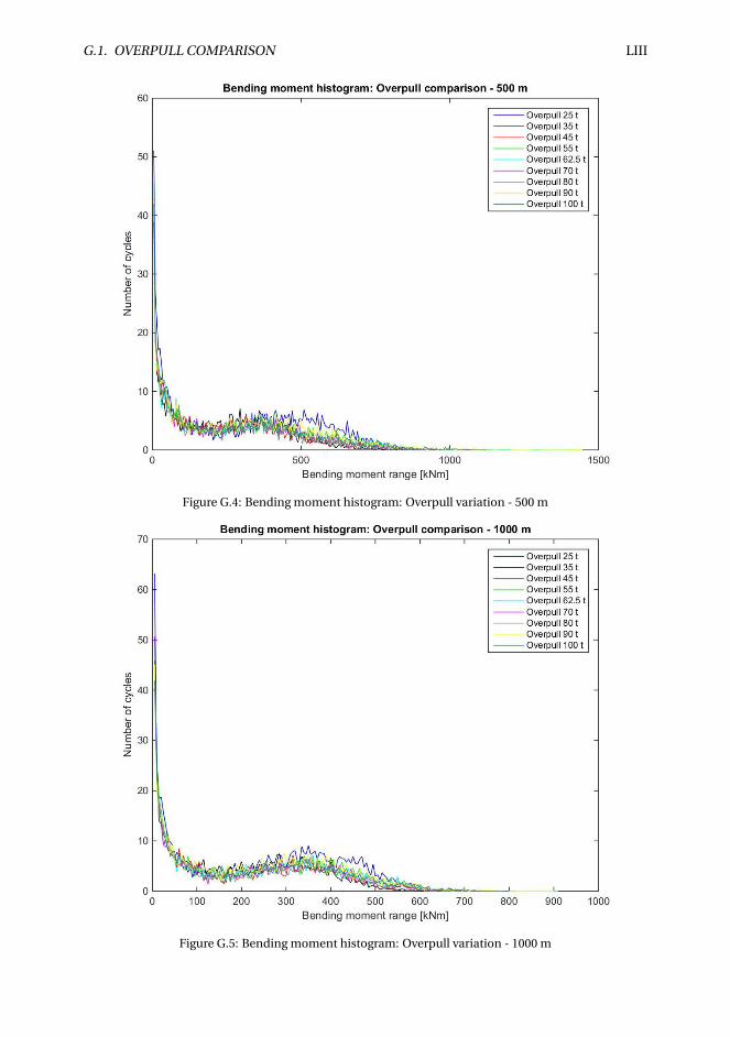
G.1. OVERPULL COMPARISON LIII
Figure G.4: Bending moment histogram: Overpull variation - 500 m
Figure G.5: Bending moment histogram: Overpull variation - 1000 m
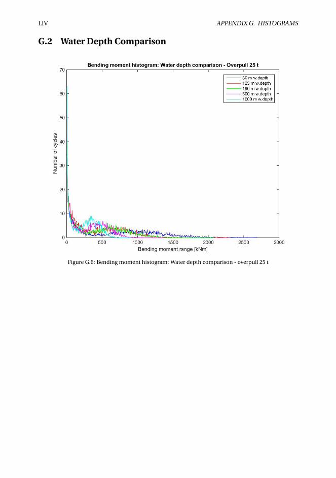
LIV APPENDIX G. HISTOGRAMS
G.2 Water Depth Comparison
Figure G.6: Bending moment histogram: Water depth comparison - overpull 25 t
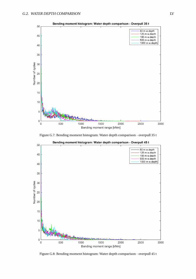
G.2. WATER DEPTH COMPARISON LV
Figure G.7: Bending moment histogram: Water depth comparison - overpull 35 t
Figure G.8: Bending moment histogram: Water depth comparison - overpull 45 t
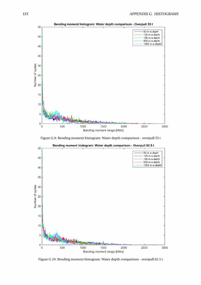
LVI APPENDIX G. HISTOGRAMS
Figure G.9: Bending moment histogram: Water depth comparison - overpull 55 t
Figure G.10: Bending moment histogram: Water depth comparison - overpull 62.5 t
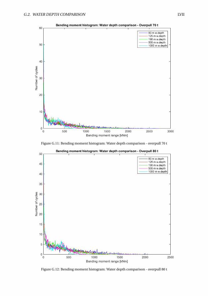
G.2. WATER DEPTH COMPARISON LVII
Figure G.11: Bending moment histogram: Water depth comparison - overpull 70 t
Figure G.12: Bending moment histogram: Water depth comparison - overpull 80 t
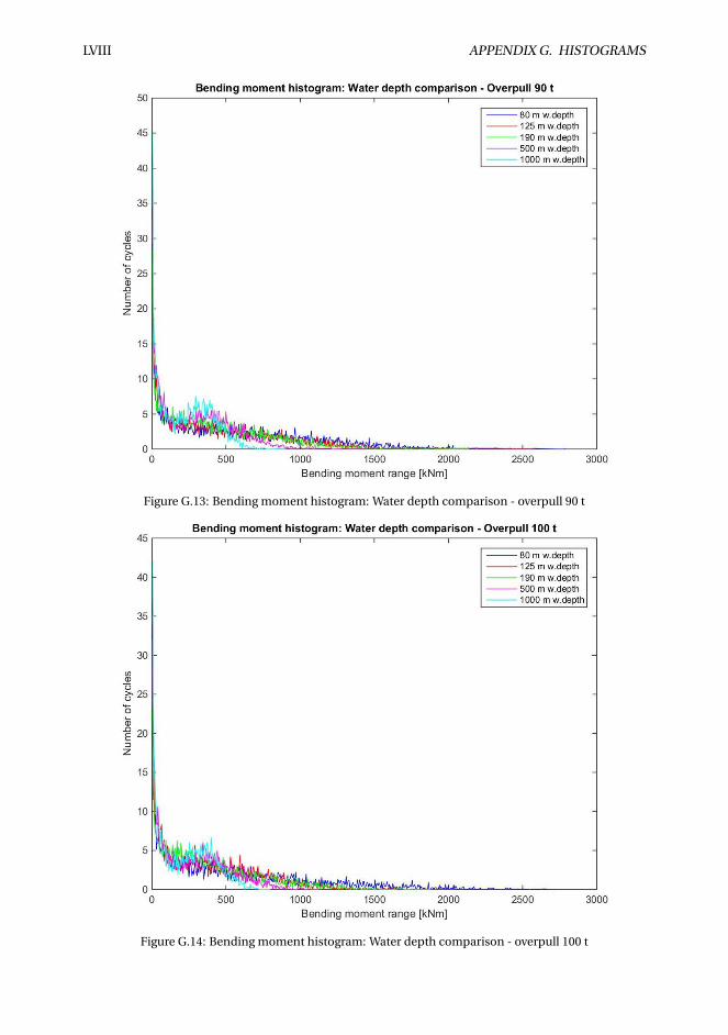
LVIII APPENDIX G. HISTOGRAMS
Figure G.13: Bending moment histogram: Water depth comparison - overpull 90 t
Figure G.14: Bending moment histogram: Water depth comparison - overpull 100 t
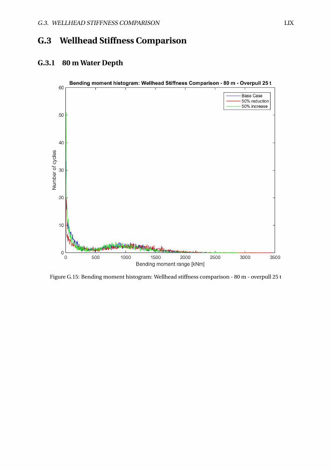
G.3. WELLHEAD STIFFNESS COMPARISON LIX
G.3 Wellhead Stiffness Comparison
G.3.1 80 m Water Depth
Figure G.15: Bending moment histogram: Wellhead stiffness comparison - 80 m - overpull 25 t
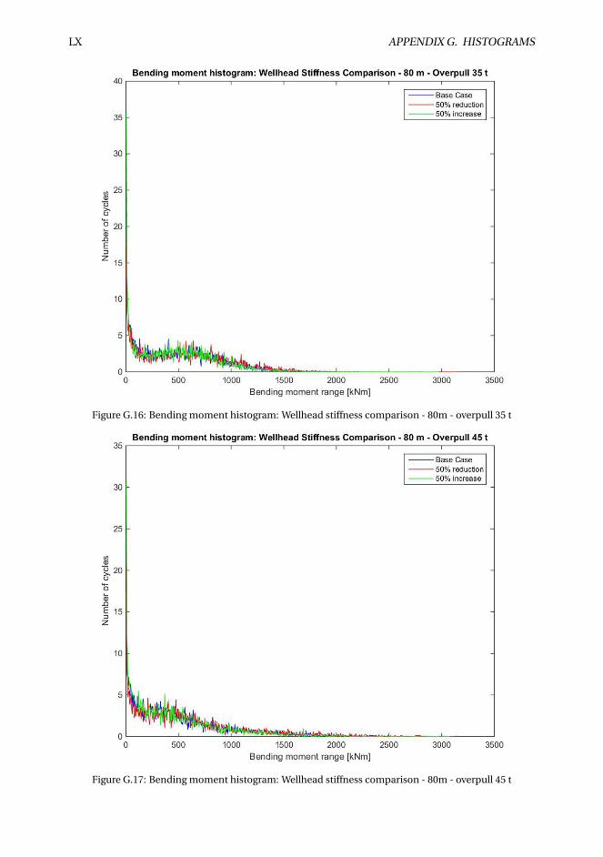
LX APPENDIX G. HISTOGRAMS
Figure G.16: Bending moment histogram: Wellhead stiffness comparison - 80m - overpull 35 t
Figure G.17: Bending moment histogram: Wellhead stiffness comparison - 80m - overpull 45 t
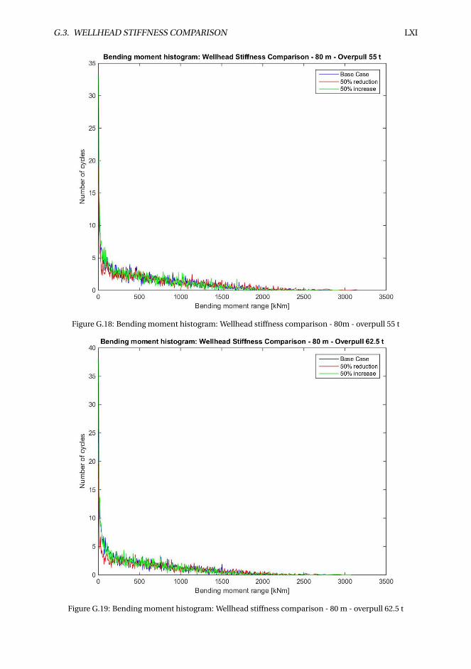
G.3. WELLHEAD STIFFNESS COMPARISON LXI
Figure G.18: Bending moment histogram: Wellhead stiffness comparison - 80m - overpull 55 t
Figure G.19: Bending moment histogram: Wellhead stiffness comparison - 80 m - overpull 62.5 t
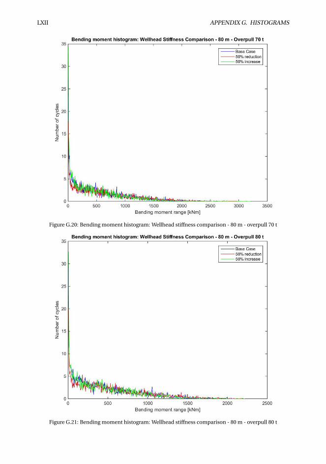
LXII APPENDIX G. HISTOGRAMS
Figure G.20: Bending moment histogram: Wellhead stiffness comparison - 80 m - overpull 70 t
Figure G.21: Bending moment histogram: Wellhead stiffness comparison - 80 m - overpull 80 t
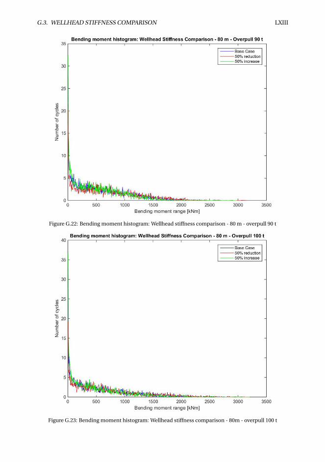
G.3. WELLHEAD STIFFNESS COMPARISON LXIII
Figure G.22: Bending moment histogram: Wellhead stiffness comparison - 80 m - overpull 90 t
Figure G.23: Bending moment histogram: Wellhead stiffness comparison - 80m - overpull 100 t
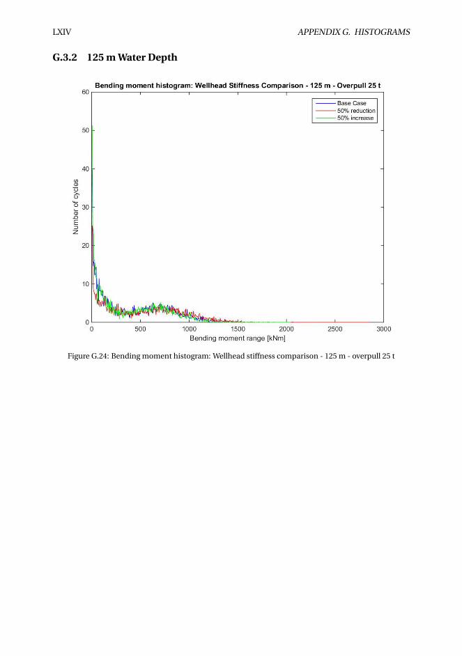
LXIV APPENDIX G. HISTOGRAMS
G.3.2 125 m Water Depth
Figure G.24: Bending moment histogram: Wellhead stiffness comparison - 125 m - overpull 25 t
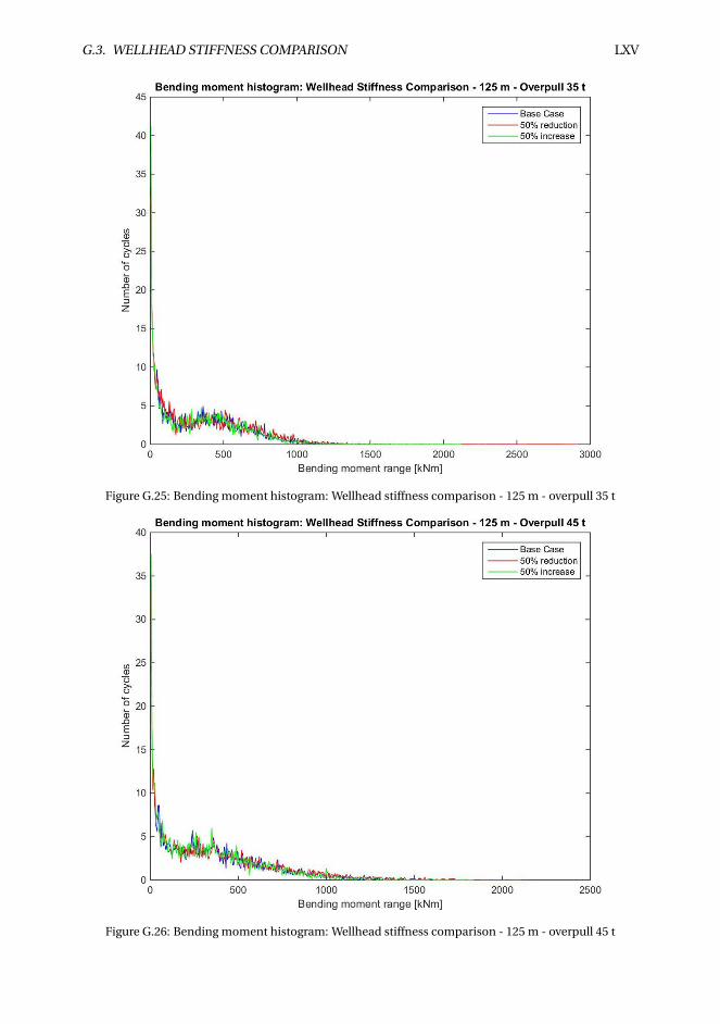
G.3. WELLHEAD STIFFNESS COMPARISON LXV
Figure G.25: Bending moment histogram: Wellhead stiffness comparison - 125 m - overpull 35 t
Figure G.26: Bending moment histogram: Wellhead stiffness comparison - 125 m - overpull 45 t
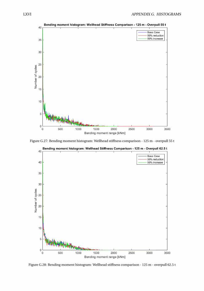
LXVI APPENDIX G. HISTOGRAMS
Figure G.27: Bending moment histogram: Wellhead stiffness comparison - 125 m - overpull 55 t
Figure G.28: Bending moment histogram: Wellhead stiffness comparison - 125 m - overpull 62.5 t
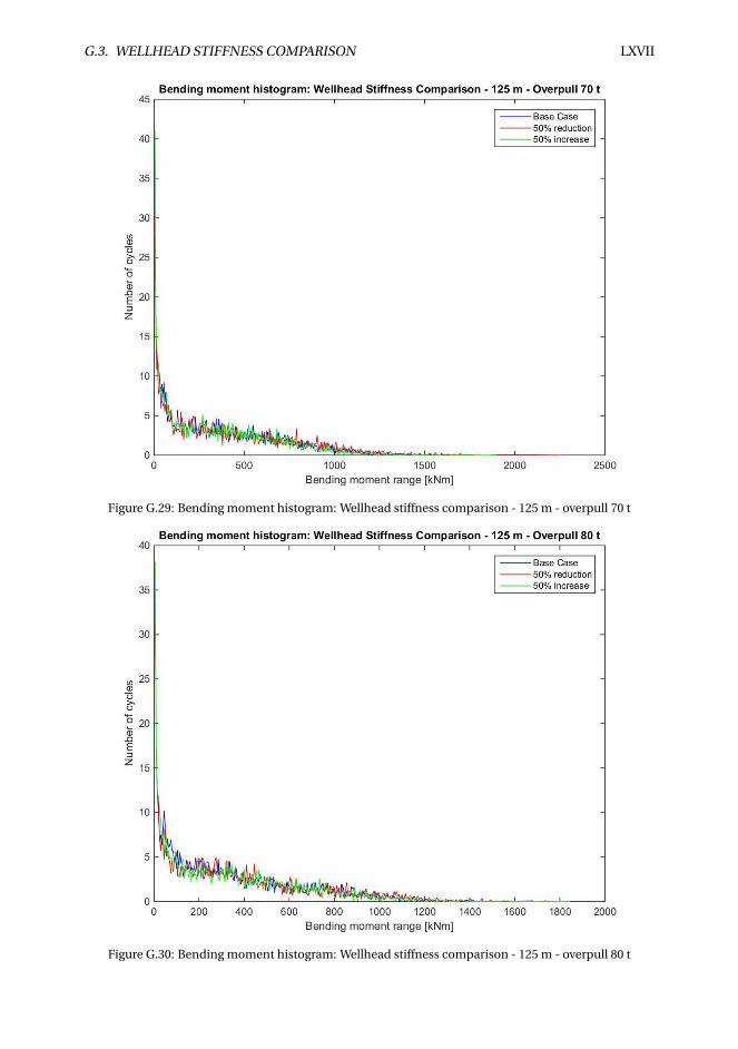
G.3. WELLHEAD STIFFNESS COMPARISON LXVII
Figure G.29: Bending moment histogram: Wellhead stiffness comparison - 125 m - overpull 70 t
Figure G.30: Bending moment histogram: Wellhead stiffness comparison - 125 m - overpull 80 t
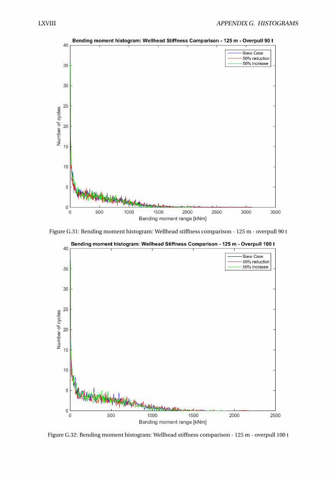
LXVIII APPENDIX G. HISTOGRAMS
Figure G.31: Bending moment histogram: Wellhead stiffness comparison - 125 m - overpull 90 t
Figure G.32: Bending moment histogram: Wellhead stiffness comparison - 125 m - overpull 100 t
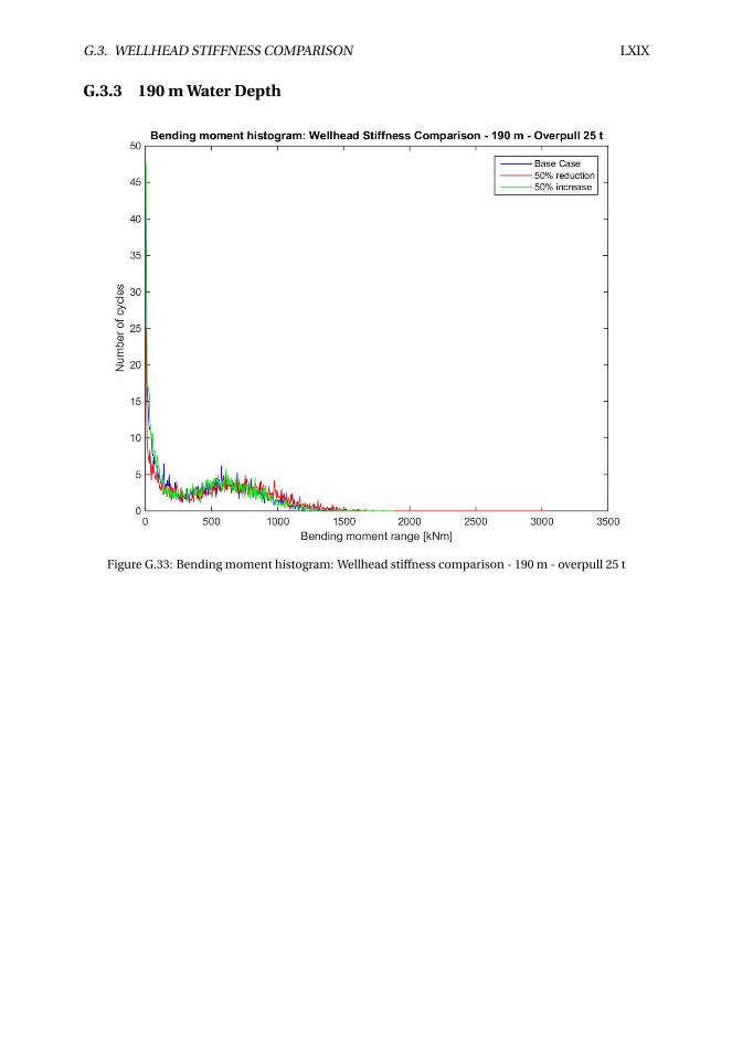
G.3. WELLHEAD STIFFNESS COMPARISON LXIX
G.3.3 190 m Water Depth
Figure G.33: Bending moment histogram: Wellhead stiffness comparison - 190 m - overpull 25 t
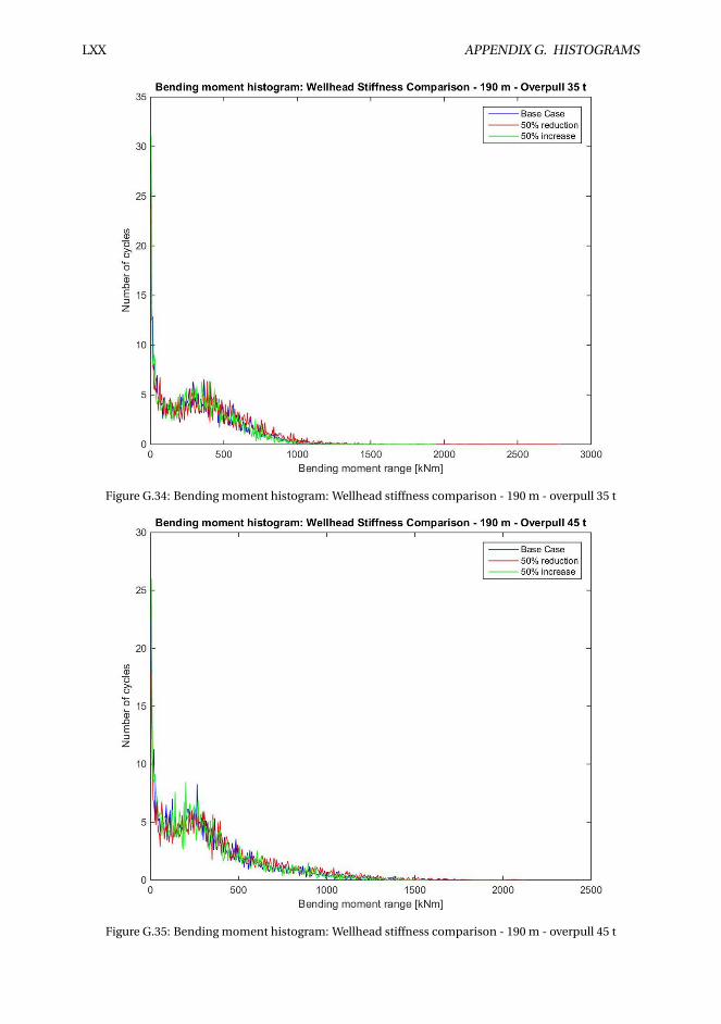
LXX APPENDIX G. HISTOGRAMS
Figure G.34: Bending moment histogram: Wellhead stiffness comparison - 190 m - overpull 35 t
Figure G.35: Bending moment histogram: Wellhead stiffness comparison - 190 m - overpull 45 t
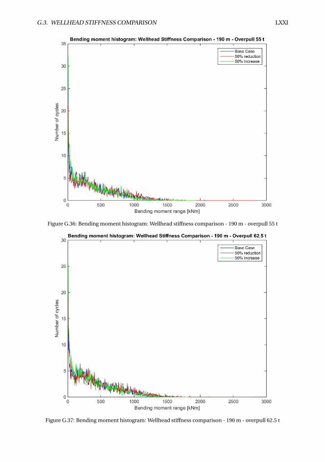
G.3. WELLHEAD STIFFNESS COMPARISON LXXI
Figure G.36: Bending moment histogram: Wellhead stiffness comparison - 190 m - overpull 55 t
Figure G.37: Bending moment histogram: Wellhead stiffness comparison - 190 m - overpull 62.5 t
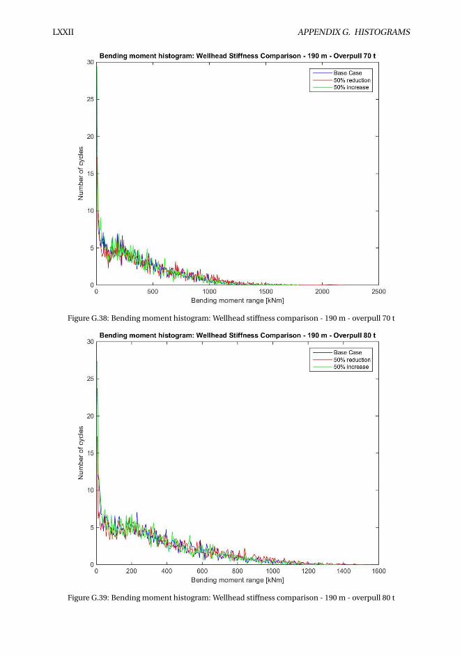
LXXII APPENDIX G. HISTOGRAMS
Figure G.38: Bending moment histogram: Wellhead stiffness comparison - 190 m - overpull 70 t
Figure G.39: Bending moment histogram: Wellhead stiffness comparison - 190 m - overpull 80 t
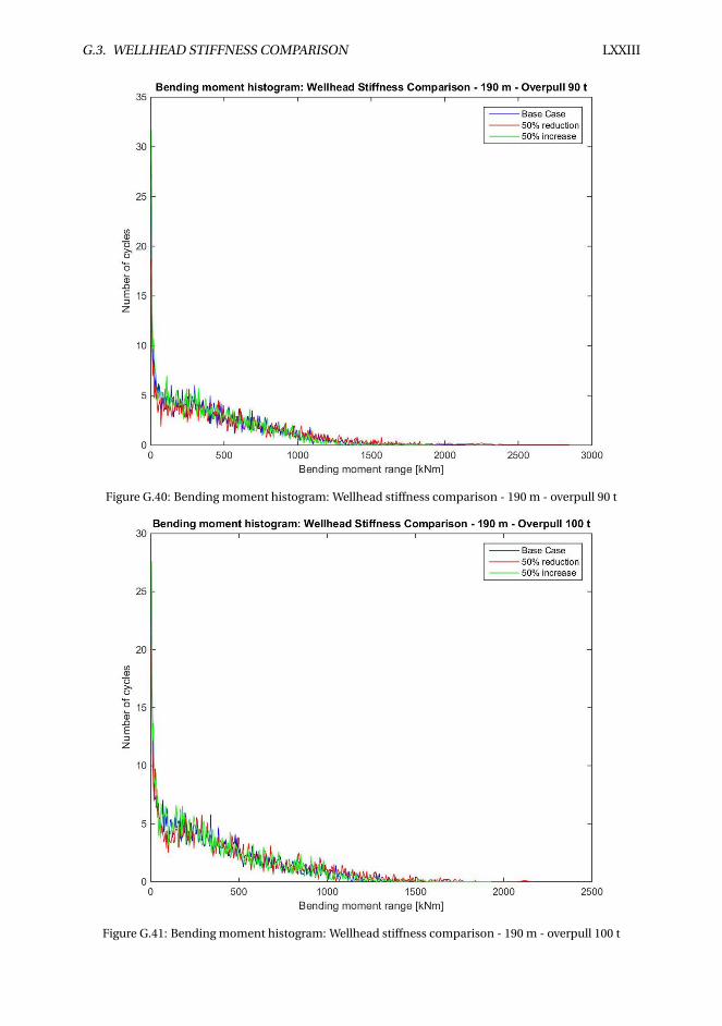
G.3. WELLHEAD STIFFNESS COMPARISON LXXIII
Figure G.40: Bending moment histogram: Wellhead stiffness comparison - 190 m - overpull 90 t
Figure G.41: Bending moment histogram: Wellhead stiffness comparison - 190 m - overpull 100 t
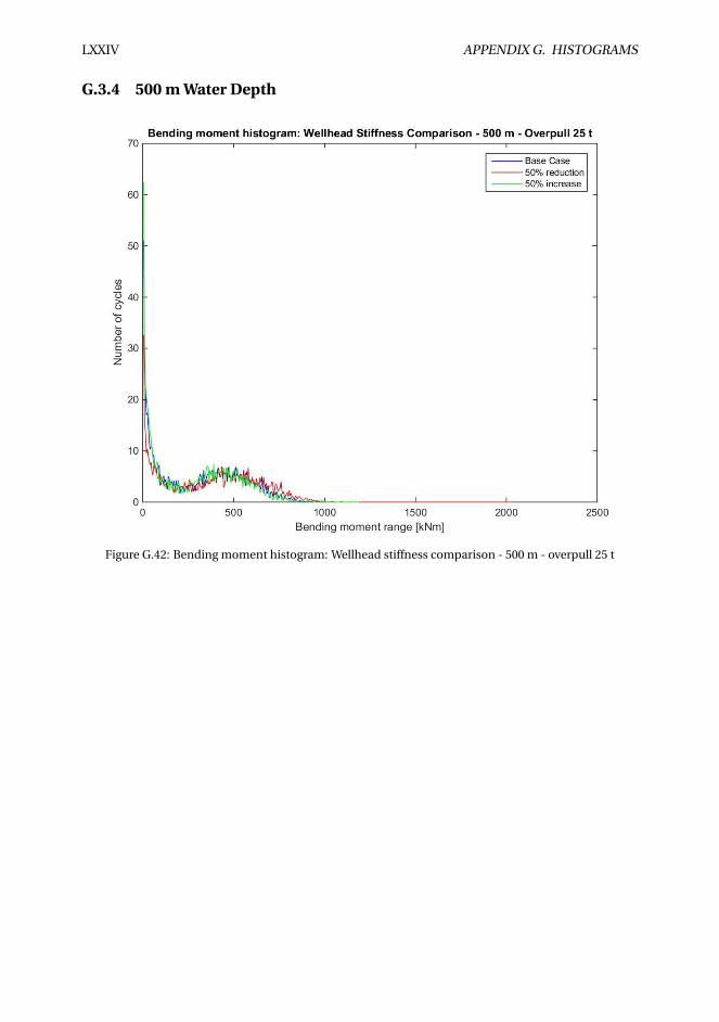
LXXIV APPENDIX G. HISTOGRAMS
G.3.4 500 m Water Depth
Figure G.42: Bending moment histogram: Wellhead stiffness comparison - 500 m - overpull 25 t
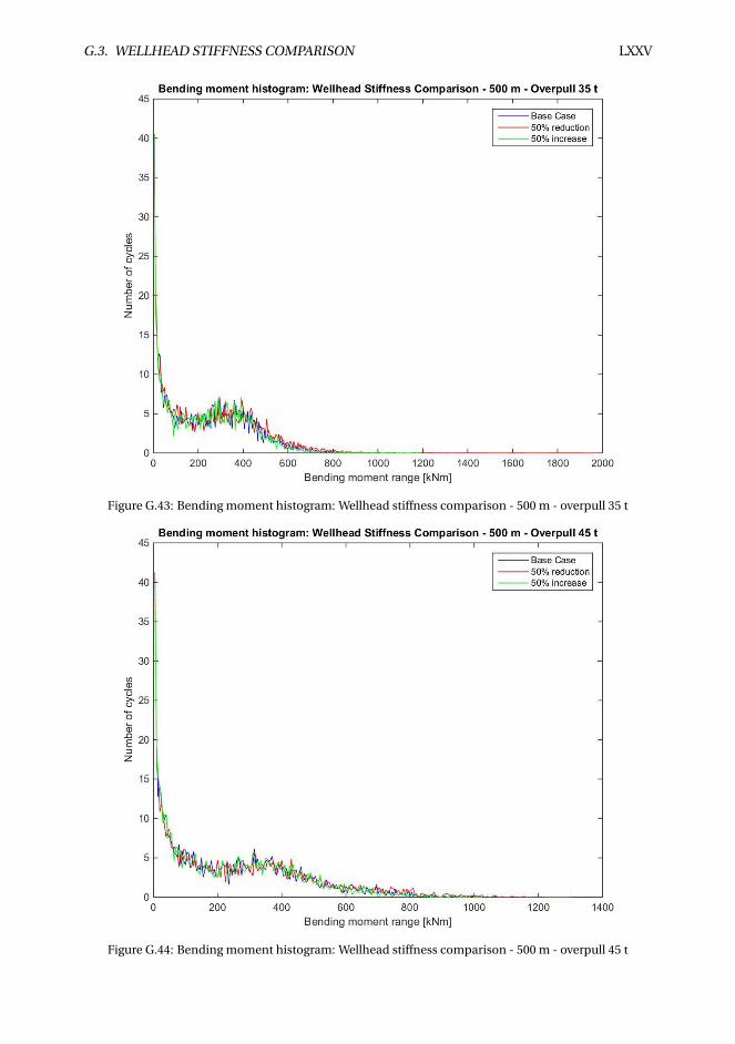
G.3. WELLHEAD STIFFNESS COMPARISON LXXV
Figure G.43: Bending moment histogram: Wellhead stiffness comparison - 500 m - overpull 35 t
Figure G.44: Bending moment histogram: Wellhead stiffness comparison - 500 m - overpull 45 t
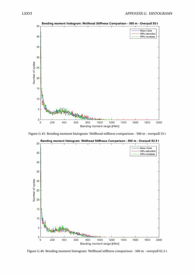
LXXVI APPENDIX G. HISTOGRAMS
Figure G.45: Bending moment histogram: Wellhead stiffness comparison - 500 m - overpull 55 t
Figure G.46: Bending moment histogram: Wellhead stiffness comparison - 500 m - overpull 62.5 t
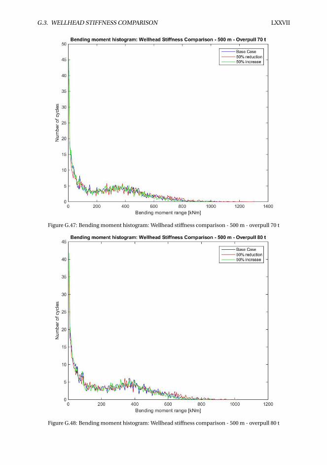
G.3. WELLHEAD STIFFNESS COMPARISON LXXVII
Figure G.47: Bending moment histogram: Wellhead stiffness comparison - 500 m - overpull 70 t
Figure G.48: Bending moment histogram: Wellhead stiffness comparison - 500 m - overpull 80 t
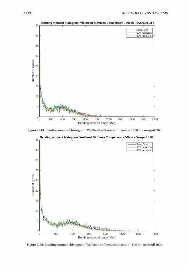
LXXVIII APPENDIX G. HISTOGRAMS
Figure G.49: Bending moment histogram: Wellhead stiffness comparison - 500 m - overpull 90 t
Figure G.50: Bending moment histogram: Wellhead stiffness comparison - 500 m - overpull 100 t
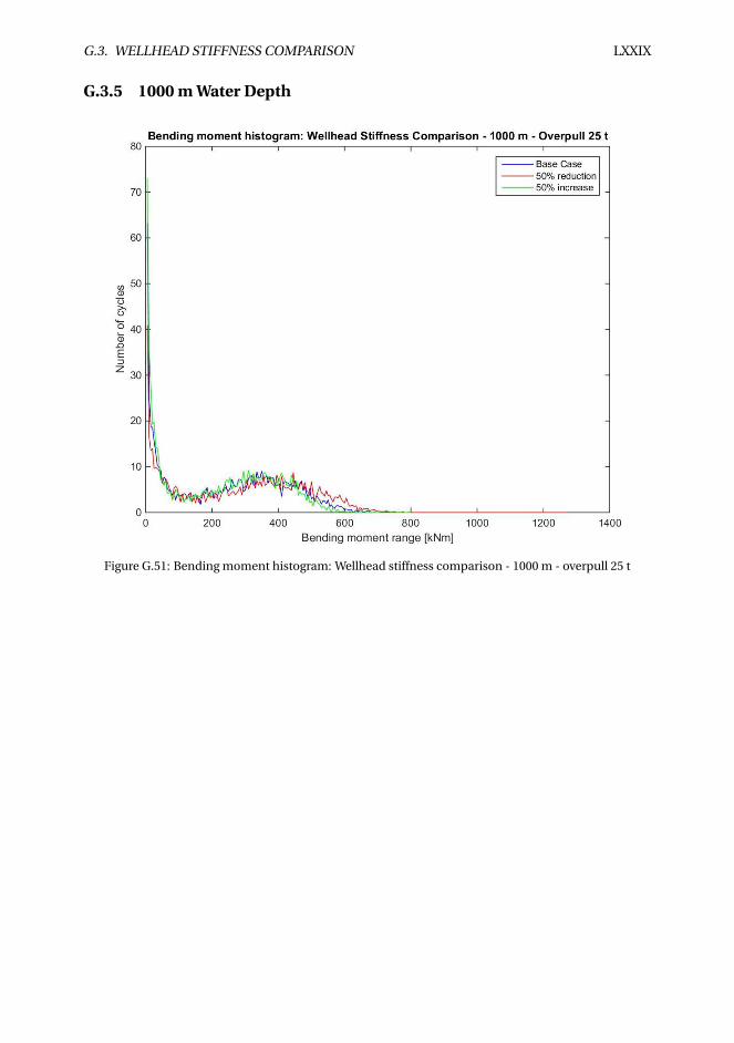
G.3. WELLHEAD STIFFNESS COMPARISON LXXIX
G.3.5 1000 m Water Depth
Figure G.51: Bending moment histogram: Wellhead stiffness comparison - 1000 m - overpull 25 t
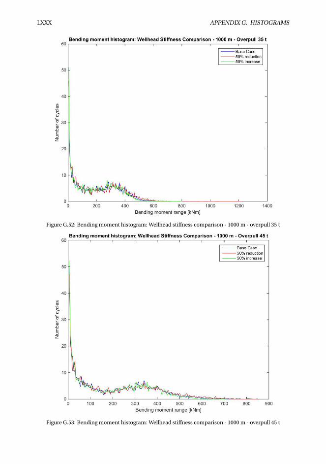
LXXX APPENDIX G. HISTOGRAMS
Figure G.52: Bending moment histogram: Wellhead stiffness comparison - 1000 m - overpull 35 t
Figure G.53: Bending moment histogram: Wellhead stiffness comparison - 1000 m - overpull 45 t
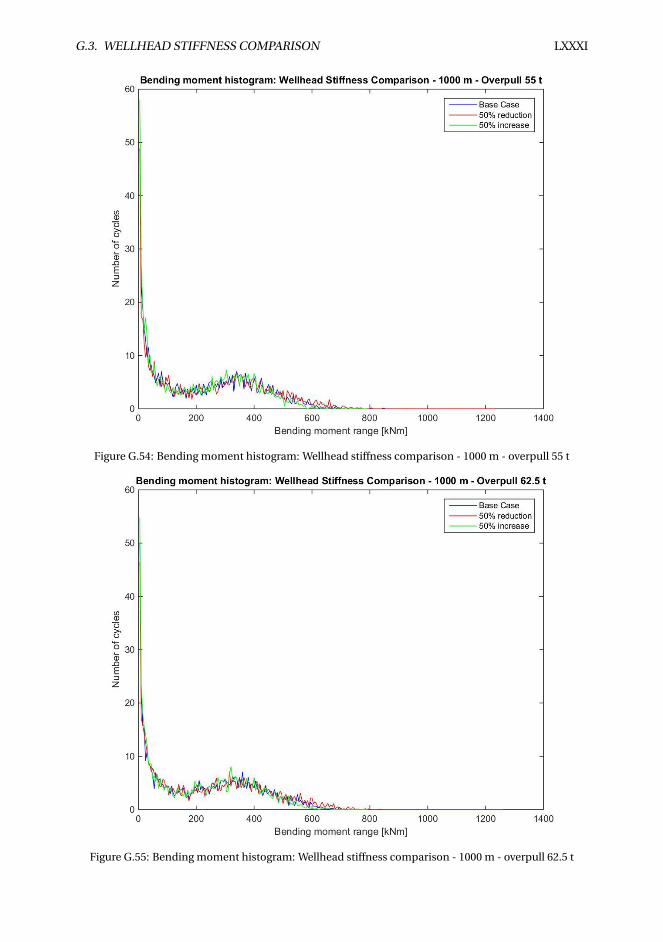
G.3. WELLHEAD STIFFNESS COMPARISON LXXXI
Figure G.54: Bending moment histogram: Wellhead stiffness comparison - 1000 m - overpull 55 t
Figure G.55: Bending moment histogram: Wellhead stiffness comparison - 1000 m - overpull 62.5 t
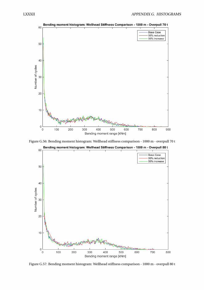
LXXXII APPENDIX G. HISTOGRAMS
Figure G.56: Bending moment histogram: Wellhead stiffness comparison - 1000 m - overpull 70 t
Figure G.57: Bending moment histogram: Wellhead stiffness comparison - 1000 m - overpull 80 t
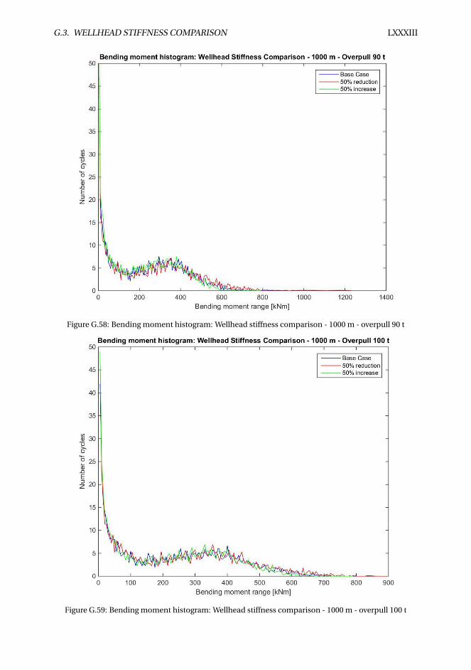
G.3. WELLHEAD STIFFNESS COMPARISON LXXXIII
Figure G.58: Bending moment histogram: Wellhead stiffness comparison - 1000 m - overpull 90 t
Figure G.59: Bending moment histogram: Wellhead stiffness comparison - 1000 m - overpull 100 t

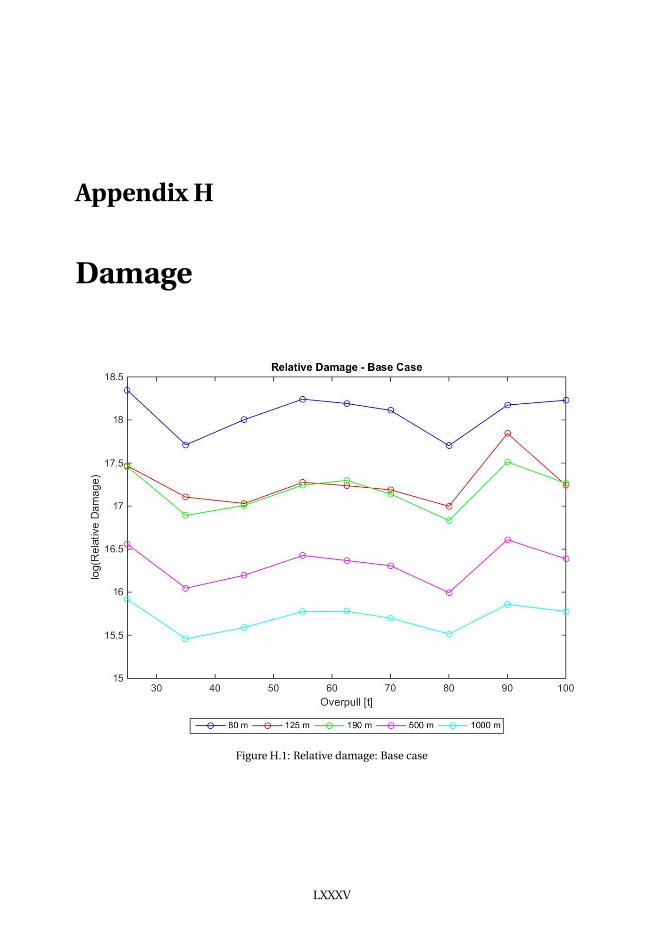
Appendix H
Damage
Figure H.1: Relative damage: Base case
LXXXV
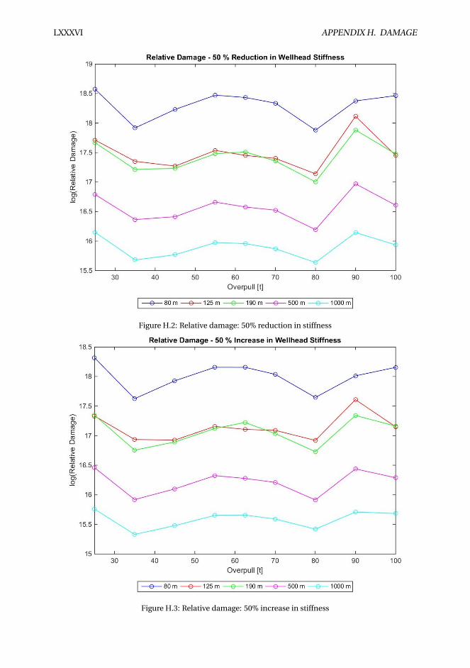
LXXXVI APPENDIX H. DAMAGE
Figure H.2: Relative damage: 50% reduction in stiffness
Figure H.3: Relative damage: 50% increase in stiffness
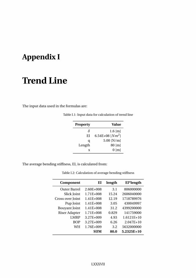
Appendix I
Trend Line
The input data used in the formulas are:
Table I.1: Input data for calculation of trend line
Property Value
δ 1.6 [m]EI 6.54E+08 [N m2]q 5.00 [N/m]
Length 80 [m]x 0 [m]
The average bending stiffness, EI, is calculated from:
Table I.2: Calculation of average bending stiffness
Component EI length EI*length
Outer Barrel 2.60E+008 3.1 806000000Slick Joint 1.71E+008 15.24 2606040000
Cross over Joint 1.41E+008 12.19 1718789976Pup Joint 1.41E+008 3.05 430049997
Bouyant Joint 1.41E+008 31.2 4399200000Riser Adapter 1.71E+008 0.829 141759000
LMRP 3.27E+009 4.93 1.6121E+10BOP 3.27E+009 6.26 2.047E+10WH 1.76E+009 3.2 5632000000
SUM 80.0 5.2325E+10
LXXXVII

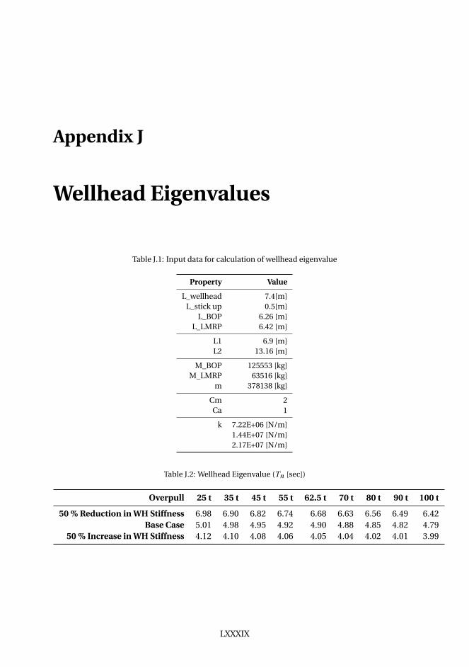
Appendix J
Wellhead Eigenvalues
Table J.1: Input data for calculation of wellhead eigenvalue
Property Value
L_wellhead 7.4[m]L_stick up 0.5[m]
L_BOP 6.26 [m]L_LMRP 6.42 [m]
L1 6.9 [m]L2 13.16 [m]
M_BOP 125553 [kg]M_LMRP 63516 [kg]
m 378138 [kg]
Cm 2Ca 1
k 7.22E+06 [N/m]1.44E+07 [N/m]2.17E+07 [N/m]
Table J.2: Wellhead Eigenvalue (Tn [sec])
Overpull 25 t 35 t 45 t 55 t 62.5 t 70 t 80 t 90 t 100 t
50 % Reduction in WH Stiffness 6.98 6.90 6.82 6.74 6.68 6.63 6.56 6.49 6.42Base Case 5.01 4.98 4.95 4.92 4.90 4.88 4.85 4.82 4.79
50 % Increase in WH Stiffness 4.12 4.10 4.08 4.06 4.05 4.04 4.02 4.01 3.99
LXXXIX


Appendix K
Contents in Attached Zip-file
This is an overview of the files attached in the zip-file.
SIMA/RIFLEXdrillingriser.stask contains the set up and anlyses of the five different water depths. To check
the effect of wellhead stiffness the global spring value is changed manually. All sensitivity stud-
ies is also carried out with manually changing the property.
MATLABrainflowcount_ withdamage.m is the matlabfile that calculates the relative fatigue damage and
produces histograms. To run the file the WAFO package has to be installed on the computer.
Exceleigenvalue_ basecase.xlsx, eigenvalue_ 50%increasedstiffness.xlsx & eigenvalue_ 50%reduced-
stiffness.xlsx contains all eigenvalues for the different loadcases. WH_ local_ eigenvalue.xlsx
contains the eigenvalues calculated analytically for the wellhead.
tensioncalculation.xlsx contains the calculation of applied top-tension for all the loadcases.
trendline.xlsx is the calculation for the trendline proposed.
damage.xlsx contains fatigue damage for all cases investigated (calculated in MATLAB).
OtherPOSTER_ KG.pdf is the poster delivered for the poster exhibition at NTNU, 26th-28th of may.
XCI
Related Documents