FRBNY ECONOMIC POLICY REVIEW /APRIL 1996 39 R Evaluation of Value-at-Risk Models Using Historical Data Darryll Hendricks esearchers in the field of financial economics have long recognized the importance of mea- suring the risk of a portfolio of financial assets or securities. Indeed, concerns go back at least four decades, when Markowitz’s pioneering work on portfolio selection (1959) explored the appropriate defi- nition and measurement of risk. In recent years, the growth of trading activity and instances of financial market instability have prompted new studies underscoring the need for market participants to develop reliable risk mea- surement techniques. 1 One technique advanced in the literature involves the use of “value-at-risk” models. These models measure the market, or price, risk of a portfolio of financial assets—that is, the risk that the market value of the portfolio will decline as a result of changes in interest rates, foreign exchange rates, equity prices, or commodity prices. Value- at-risk models aggregate the several components of price risk into a single quantitative measure of the potential for losses over a specified time horizon. These models are clearly appealing because they convey the market risk of the entire portfolio in one number. Moreover, value-at-risk measures focus directly, and in dollar terms, on a major reason for assessing risk in the first place—a loss of portfolio value. Recognition of these models by the financial and regulatory communities is evidence of their growing use. For example, in its recent risk-based capital proposal (1996a), the Basle Committee on Banking Supervision endorsed the use of such models, contingent on important qualitative and quantitative standards. In addition, the Bank for International Settlements Fisher report (1994) urged financial intermediaries to disclose measures of value-at-risk publicly. The Derivatives Policy Group, affili- ated with six large U.S. securities firms, has also advocated the use of value-at-risk models as an important way to measure market risk. The introduction of the RiskMetrics database compiled by J.P. Morgan for use with third-party value-at-risk software also highlights the growing use of these models by financial as well as nonfinancial firms. Clearly, the use of value-at-risk models is increas- The views expressed in this article are those of the authors and do not necessarily reflect the position of the Federal Reserve Bank of New York or the Federal Reserve System. The Federal Reserve Bank of New York provides no warranty, express or implied, as to the accuracy, timeliness, com- pleteness, merchantability, or fitness for any particular purpose of any information contained in documents produced and provided by the Federal Reserve Bank of New York in any form or manner whatsoever.

Welcome message from author
This document is posted to help you gain knowledge. Please leave a comment to let me know what you think about it! Share it to your friends and learn new things together.
Transcript

FRBNY ECONOMIC POLICY REVIEW / APRIL 1996 39
R
Evaluation of Value-at-Risk ModelsUsing Historical DataDarryll Hendricks
esearchers in the field of financial economics
have long recognized the importance of mea-
suring the risk of a portfolio of financial
assets or securities. Indeed, concerns go back
at least four decades, when Markowitz’s pioneering work
on portfolio selection (1959) explored the appropriate defi-
nition and measurement of risk. In recent years, the
growth of trading activity and instances of financial market
instability have prompted new studies underscoring the
need for market participants to develop reliable risk mea-
surement techniques.1
One technique advanced in the literature involves
the use of “value-at-risk” models. These models measure the
market, or price, risk of a portfolio of financial assets—that
is, the risk that the market value of the portfolio will
decline as a result of changes in interest rates, foreign
exchange rates, equity prices, or commodity prices. Value-
at-risk models aggregate the several components of price
risk into a single quantitative measure of the potential for
losses over a specified time horizon. These models are clearly
appealing because they convey the market risk of the entire
portfolio in one number. Moreover, value-at-risk measures
focus directly, and in dollar terms, on a major reason for
assessing risk in the first place—a loss of portfolio value.
Recognition of these models by the financial and
regulatory communities is evidence of their growing use.
For example, in its recent risk-based capital proposal
(1996a), the Basle Committee on Banking Supervision
endorsed the use of such models, contingent on important
qualitative and quantitative standards. In addition, the
Bank for International Settlements Fisher report (1994)
urged financial intermediaries to disclose measures of
value-at-risk publicly. The Derivatives Policy Group, affili-
ated with six large U.S. securities firms, has also advocated
the use of value-at-risk models as an important way to
measure market risk. The introduction of the RiskMetrics
database compiled by J.P. Morgan for use with third-party
value-at-risk software also highlights the growing use of
these models by financial as well as nonfinancial firms.
Clearly, the use of value-at-risk models is increas-
The views expressed in this article are those of the authors and do not necessarily reflect the position of the Federal
Reserve Bank of New York or the Federal Reserve System.
The Federal Reserve Bank of New York provides no warranty, express or implied, as to the accuracy, timeliness, com-
pleteness, merchantability, or fitness for any particular purpose of any information contained in documents produced
and provided by the Federal Reserve Bank of New York in any form or manner whatsoever.

40 FRBNY ECONOMIC POLICY REVIEW / APRIL 1996
ing, but how well do they perform in practice? This article
explores this question by applying value-at-risk models to
1,000 randomly chosen foreign exchange portfolios over
the period 1983-94. We then use nine criteria to evaluate
model performance. We consider, for example, how closely
risk measures produced by the models correspond to actual
portfolio outcomes.
We begin by explaining the three most common
categories of value-at-risk models—equally weighted mov-
ing average approaches, exponentially weighted moving
average approaches, and historical simulation approaches.
Although within these three categories many different
approaches exist, for the purposes of this article we select five
approaches from the first category, three from the second,
and four from the third.
By employing a simulation technique using these
twelve value-at-risk approaches, we arrived at measures of
price risk for the portfolios at both 95 percent and 99 per-
cent confidence levels over one-day holding periods. The con-
fidence levels specify the probability that losses of a
portfolio will be smaller than estimated by the risk mea-
sure. Although this article considers value-at-risk models
only in the context of market risk, the methodology is
fairly general and could in theory address any source of risk
that leads to a decline in market values. An important lim-
itation of the analysis, however, is that it does not consider
portfolios containing options or other positions with non-
linear price behavior.2
We choose several performance criteria to reflect
the practices of risk managers who rely on value-at-risk
measures for many purposes. Although important differ-
ences emerge across value-at-risk approaches with respect
to each criterion, the results indicate that none of the
twelve approaches we examine is superior on every count.
In addition, as the results make clear, the choice of confi-
dence level—95 percent or 99 percent—can have a sub-
stantial effect on the performance of value-at-risk
approaches.
INTRODUCTION TO VALUE-AT-RISK MODELS
A value-at-risk model measures market risk by determin-
ing how much the value of a portfolio could decline over a
given period of time with a given probability as a result of
changes in market prices or rates. For example, if the
given period of time is one day and the given probability
is 1 percent, the value-at-risk measure would be an estimate
of the decline in the portfolio value that could occur with a
1 percent probability over the next trading day. In other
words, if the value-at-risk measure is accurate, losses
greater than the value-at-risk measure should occur less
than 1 percent of the time.
The two most important components of value-at-
risk models are the length of time over which market risk is
to be measured and the confidence level at which market risk
is measured. The choice of these components by risk manag-
ers greatly affects the nature of the value-at-risk model.
The time period used in the definition of value-at-
risk, often referred to as the “holding period,” is discretion-
ary. Value-at-risk models assume that the portfolio’s com-
position does not change over the holding period. This
assumption argues for the use of short holding periods
because the composition of active trading portfolios is apt
to change frequently. Thus, this article focuses on the
widely used one-day holding period.3
Value-at-risk measures are most often expressed as
percentiles corresponding to the desired confidence level.
For example, an estimate of risk at the 99 percent confi-
dence level is the amount of loss that a portfolio is
expected to exceed only 1 percent of the time. It is also
known as a 99th percentile value-at-risk measure because
the amount is the 99th percentile of the distribution of
potential losses on the portfolio.4 In practice, value-at-risk
estimates are calculated from the 90th to 99.9th percen-
tiles, but the most commonly used range is the 95th to
99th percentile range. Accordingly, the text charts and the
Clearly, the use of value-at-risk models is
increasing, but how well do they
perform in practice?
FRBNY ECONOMIC POLICY REVIEW / APRIL 1996 41
tables in the appendix report simulation results for each of
these percentiles.
THREE CATEGORIES OF VALUE-AT-RISK
APPROACHES
Although risk managers apply many approaches when cal-
culating portfolio value-at-risk models, almost all use past
data to estimate potential changes in the value of the port-
folio in the future. Such approaches assume that the future
will be like the past, but they often define the past quite
differently and make different assumptions about how
markets will behave in the future.
The first two categories we examine, “variance-
covariance” value-at-risk approaches,5 assume normality
and serial independence and an absence of nonlinear posi-
tions such as options.6 The dual assumption of normality
and serial independence creates ease of use for two reasons.
First, normality simplifies value-at-risk calculations
because all percentiles are assumed to be known multiples
of the standard deviation. Thus, the value-at-risk calcula-
tion requires only an estimate of the standard deviation of
the portfolio’s change in value over the holding period.
Second, serial independence means that the size of a price
move on one day will not affect estimates of price moves on
any other day. Consequently, longer horizon standard devi-
ations can be obtained by multiplying daily horizon stan-
dard deviations by the square root of the number of days in
the longer horizon. When the assumptions of normality
and serial independence are made together, a risk manager
can use a single calculation of the portfolio’s daily horizon
standard deviation to develop value-at-risk measures for
any given holding period and any given percentile.
The advantages of these assumptions, however,
must be weighed against a large body of evidence suggest-
ing that the tails of the distributions of daily percentage
changes in financial market prices, particularly foreign
exchange rates, will be fatter than predicted by the normal
distribution.7 This evidence calls into question the appeal-
ing features of the normality assumption, especially for
value-at-risk measurement, which focuses on the tails of
the distribution. Questions raised by the commonly used
normality assumption are highlighted throughout the article.
In the sections below, we describe the individual
features of the two variance-covariance approaches to value-
at-risk measurement.
EQUALLY WEIGHTED MOVING AVERAGE
APPROACHES
The equally weighted moving average approach, the more
straightforward of the two, calculates a given portfolio’s
variance (and thus, standard deviation) using a fixed
amount of historical data.8 The major difference among
equally weighted moving average approaches is the time
frame of the fixed amount of data.9 Some approaches
employ just the most recent fifty days of historical data on
the assumption that only very recent data are relevant to
estimating potential movements in portfolio value. Other
approaches assume that large amounts of data are necessary
to estimate potential movements accurately and thus rely
on a much longer time span—for example, five years.
The calculation of portfolio standard deviations
using an equally weighted moving average approach is
(1) ,
where denotes the estimated standard deviation of the
portfolio at the beginning of day t. The parameter k speci-
fies the number of days included in the moving average
(the “observation period”), xs, the change in portfolio value
on day s, and , the mean change in portfolio value. Fol-
lowing the recommendation of Figlewski (1994), is
always assumed to be zero.10
Consider five sets of value-at-risk measures with
periods of 50, 125, 250, 500, and 1,250 days, or about two
months, six months, one year, two years, and five years of
historical data. Using three of these five periods of time,
Chart 1 plots the time series of value-at-risk measures at
biweekly intervals for a single fixed portfolio of spot for-
eign exchange positions from 1983 to 1994.11 As shown,
the fifty-day risk measures are prone to rapid swings. Con-
versely, the 1,250-day risk measures are more stable over
long periods of time, and the behavior of the 250-day risk
measures lies somewhere in the middle.
σt1
k 1–( )---------------- xs µ–( )2
s t k–=
t 1–
∑=
σt
µ
µ

42 FRBNY ECONOMIC POLICY REVIEW / APRIL 1996
EXPONENTIALLY WEIGHTED MOVING AVERAGE
APPROACHES
Exponentially weighted moving average approaches
emphasize recent observations by using exponentially
weighted moving averages of squared deviations. In con-
trast to equally weighted approaches, these approaches
attach different weights to the past observations contained
in the observation period. Because the weights decline
exponentially, the most recent observations receive much
more weight than earlier observations. The formula for the
portfolio standard deviation under an exponentially
weighted moving average approach is
(2) .
The parameter λ, referred to as the “decay factor,”
determines the rate at which the weights on past observa-
tions decay as they become more distant. In theory, for the
weights to sum to one, these approaches should use an infi-
nitely large number of observations k. In practice, for the
values of the decay factor λ considered here, the sum of the
weights will converge to one, with many fewer observa-
tions than the 1,250 days used in the simulations. As with
σt 1 λ–( ) λt s– 1– xs µ–( )2
s t k–=
t 1–
∑=
the equally weighted moving averages, the parameter is
assumed to equal zero.
Exponentially weighted moving average approaches
clearly aim to capture short-term movements in volatility,
the same motivation that has generated the large body of lit-
erature on conditional volatility forecasting models.12 In
fact, exponentially weighted moving average approaches are
equivalent to the IGARCH(1,1) family of popular condi-
tional volatility models.13 Equation 3 gives an equivalent
formulation of the model and may also suggest a more intu-
itive understanding of the role of the decay factor:
(3) .
As shown, an exponentially weighted average on
any given day is a simple combination of two components:
(1) the weighted average on the previous day, which
receives a weight of λ, and (2) yesterday’s squared devia-
tion, which receives a weight of (1 - λ). This interaction
means that the lower the decay factor λ, the faster the decay
in the influence of a given observation. This concept is
illustrated in Chart 2, which plots time series of value-at-
risk measures using exponentially weighted moving aver-
µ
σt λσt 1–2 1 λ–( )+ xt 1– µ–( )2=
Value-at-Risk Measures for a Single Portfolio over Time
Equally Weighted Moving Average Approaches
Chart 1
Millions of Dollars
1983 85
Source: Author’s� calculations.
0
2
4
6
8
10
86 87 88 89 90 91 92 93 9484 95
50 days
250 days
1,250 days

FRBNY ECONOMIC POLICY REVIEW / APRIL 1996 43
Value-at-Risk Measures for a Single Portfolio over Time
Exponentially Weighted Moving Average Approaches
Chart 2
Millions of Dollars
1983 85
Source: Author’s� calculations.
0
2
4
6
8
10
86 87 88 89 90 91 92 93 9484 95
Lambda = 0.94
Lambda = 0.99
ages with decay factors of 0.94 and 0.99. A decay factor of
0.94 implies a value-at-risk measure that is derived almost
entirely from very recent observations, resulting in the
high level of variability apparent for that particular series.
On the one hand, relying heavily on the recent
past seems crucial when trying to capture short-term
movements in actual volatility, the focus of conditional
volatility forecasting. On the other hand, the reliance on
recent data effectively reduces the overall sample size,
increasing the possibility of measurement error. In the lim-
iting case, relying only on yesterday’s observation would
produce highly variable and error-prone risk measures.
HISTORICAL SIMULATION APPROACHES
The third category of value-at-risk approaches is similar to
the equally weighted moving average category in that it
relies on a specific quantity of past historical observations
(the observation period). Rather than using these observa-
tions to calculate the portfolio’s standard deviation, how-
ever, historical simulation approaches use the actual
percentiles of the observation period as value-at-risk mea-
sures. For example, for an observation period of 500 days,
the 99th percentile historical simulation value-at-risk mea-
sure is the sixth largest loss observed in the sample of 500
outcomes (because the 1 percent of the sample that should
exceed the risk measure equates to five losses).
In other words, for these approaches, the 95th and
99th percentile value-at-risk measures will not be constant
multiples of each other. Moreover, value-at-risk measures
for holding periods other than one day will not be fixed
multiples of the one-day value-at-risk measures. Historical
simulation approaches do not make the assumptions of
normality or serial independence. However, relaxing these
assumptions also implies that historical simulation
approaches do not easily accommodate translations
between multiple percentiles and holding periods.
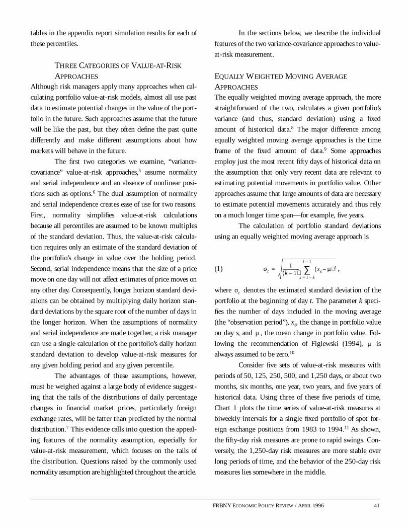
Chart 3 depicts the time series of one-day 99th
percentile value-at-risk measures calculated through his-
torical simulation. The observation periods shown are 125
days and 1,250 days.14 Interestingly, the use of actual per-
centiles produces time series with a somewhat different
appearance than is observed in either Chart 1 or Chart 2. In
particular, very abrupt shifts occur in the 99th percentile
measures for the 125-day historical simulation approach.
Trade-offs regarding the length of the observation
period for historical simulation approaches are similar to
44 FRBNY ECONOMIC POLICY REVIEW / APRIL 1996
Value-at-Risk Measures for a Single Portfolio over Time
Historical Simulation Approaches
Chart 3
Millions of Dollars
1983 85
Source: Author’s� calculations.
0
2
4
6
8
10
86 87 88 89 90 91 92 93 9484 95
125 days 1,250 days
those for variance-covariance approaches. Clearly, the
choice of 125 days is motivated by the desire to capture
short-term movements in the underlying risk of the port-
folio. In contrast, the choice of 1,250 days may be driven
by the desire to estimate the historical percentiles as accu-
rately as possible. Extreme percentiles such as the 95th and
particularly the 99th are very difficult to estimate accu-
rately with small samples. Thus, the fact that historical
simulation approaches abandon the assumption of normal-
ity and attempt to estimate these percentiles directly is one
rationale for using long observation periods.
SIMULATIONS OF VALUE-AT-RISK MODELS
This section provides an introduction to the simulation
results derived by applying twelve value-at-risk approaches
to 1,000 randomly selected foreign exchange portfolios and
assessing their behavior along nine performance criteria
(see box). This simulation design has several advantages.
First, by simulating the performance of each value-at-risk
approach for a long period of time (approximately twelve
years of daily data) and across a large number of portfolios,
we arrive at a clear picture of how value-at-risk models
would actually have performed for linear foreign exchange
portfolios over this time span. Second, the results give
insight into the extent to which portfolio composition or
choice of sample period can affect results.
It is important to emphasize, however, that nei-
ther the reported variability across portfolios nor variabil-
ity over time can be used to calculate suitable standard
errors. The appropriate standard errors for these simulation
results raise difficult questions. The results aggregate
information across multiple samples, that is, across the
1,000 portfolios. Because the results for one portfolio are
not independent of the results for other portfolios, we can-
not easily determine the total amount of information pro-
The simulation results provide a relatively
complete picture of the performance of selected
value-at-risk approaches in estimating the
market risk of a large number of portfolios.
FRBNY ECONOMIC POLICY REVIEW / APRIL 1996 45
vided by the simulations. Furthermore, many of the
performance criteria we consider do not have straightfor-
ward standard error formulas even for single samples.15
These stipulations imply that it is not possible
to use the simulation results to accept or reject specific
statistical hypotheses about these twelve value-at-risk
approaches. Moreover, the results should not in any way be
taken as indicative of the results that would be obtained for
portfolios including other financial market assets, spanning
other time periods, or looking forward. Finally, this article
does not contribute substantially to the ongoing debate
about the appropriate approach to or interpretation of
“backtesting” in conjunction with value-at-risk model-
ing.16 Despite these limitations, the simulation results do
provide a relatively complete picture of the performance of
selected value-at-risk approaches in estimating the market
risk of a large number of linear foreign exchange portfolios
over the period 1983-94.
For each of the nine performance criteria, Charts 4-12
provide a visual sense of the simulation results for 95th
and 99th percentile risk measures. In each chart, the verti-
cal axis depicts a relevant range of the performance crite-
rion under consideration (value-at-risk approaches are
arrayed horizontally across the chart). Filled circles depict
the average results across the 1,000 portfolios, and the
boxes drawn for each value-at-risk approach depict the
5th, 25th, 50th, 75th, and 95th percentiles of the distri-
bution of the results across the 1,000 portfolios.17 In some
charts, a horizontal line is drawn to highlight how the
results compare with an important point of reference.
Simulation results are also presented in tabular form in
the appendix.
DATA AND SIMULATION METHODOLOGY
This article analyzes twelve value-at-risk approaches. Theseinclude five equally weighted moving average approaches (50days, 125 days, 250 days, 500 days, 1,250 days); three expo-nentially weighted moving average approaches (λ=0.94,λ=0.97, λ=0.99); and four historical simulation approaches(125 days, 250 days, 500 days, 1,250 days).
The data consist of daily exchange rates (bid pricescollected at 4:00 p.m. New York time by the Federal ReserveBank of New York) against the U.S. dollar for the followingeight currencies: British pound, Canadian dollar, Dutch guil-der, French franc, German mark, Italian lira, Japanese yen,and Swiss franc. The historical sample covers the periodJanuary 1, 1978, to January 18, 1995 (4,255 days).
Through a simulation methodology, we attempt todetermine how each value-at-risk approach would have per-formed over a realistic range of portfolios containing the eightcurrencies over the sample period. The simulation methodol-ogy consists of five steps:
1. Select a random portfolio of positions in the eight curren-cies. This step is accomplished by drawing the position ineach currency from a uniform distribution centered onzero. In other words, the portfolio space is a uniformlydistributed eight dimensional cube centered on zero.1
2. Calculate the value-at-risk estimates for the random port-folio chosen in step one using the twelve value-at-riskapproaches for each day in the sample—day 1,251 to day4,255. In each case, we draw the historical data from the1,250 days of historical data preceding the date for whichthe calculation is made. For example, the fifty-dayequally weighted moving average estimate for a givendate would be based on the fifty days of historical datapreceding the given date.
3. Calculate the change in the portfolio’s value for each dayin the sample—again, day 1,251 to day 4,255. Withinthe article, these values are referred to as the ex post port-folio results or outcomes.
4. Assess the performance of each value-at-risk approach forthe random portfolio selected in step one by comparingthe value-at-risk estimates generated by step two withthe actual outcomes calculated in step three.
5. Repeat steps one through four 1,000 times and tabulatethe results.
1 The upper and lower bounds on the positions in each currency are +100 million U.S. dollars and -100 million U.S. dollars, respectively.In fact, however, all of the results in the article are completely invariant to the scale of the random portfolios.

46 FRBNY ECONOMIC POLICY REVIEW / APRIL 1996
Chart 4a
Percent
Mean Relative Bias
95th Percentile Value-at-Risk Measures
50d125d
250d500d
1250d λ�=0.97hs125
hs250hs500
hs1250λ�=0.94 λ�=0.99
50d125d
250d500d
1250d λ�=0.97hs125
hs250hs500
hs1250λ�=0.94 λ�=0.99
Source: Author’�s calculations.
Chart 4b
Percent
Mean Relative Bias
99th Percentile Value-at-Risk Measures
Source: Author’�s calculations.
-0.1
0
0.1
0.2
-0.2
-0.1
0
0.1
0.2
0.3
Notes: d=days; hs=historical simulation; λ=exponentially weighted. Notes: d=days; hs=historical simulation; λ=exponentially weighted.
MEAN RELATIVE BIAS
The first performance criterion we examine is whether the
different value-at-risk approaches produce risk measures of
similar average size. To ensure that the comparison is not
influenced by the scale of each simulated portfolio, we use a
four-step procedure to generate scale-free measures of the
relative sizes for each simulated portfolio.
First, we calculate value-at-risk measures for each
of the twelve approaches for the portfolio on each sample
date. Second, we average the twelve risk measures for each
date to obtain the average risk measure for that date for the
portfolio. Third, we calculate the percentage difference
between each approach’s risk measure and the average risk
measure for each date. We refer to these figures as daily rel-
ative bias figures because they are relative only to the
average risk measure across the twelve approaches rather
than to any external standard. Fourth, we average the daily
relative biases for a given value-at-risk approach across all
sample dates to obtain the approach’s mean relative bias for
the portfolio.
Intuitively, this procedure results in a measure of
size for each value-at-risk approach that is relative to the
average of all twelve approaches. The mean relative bias for
a portfolio is independent of the scale of the simulated
portfolio because each of the daily relative bias calculations
on which it is based is also scale-independent. This inde-
pendence is achieved because all of the value-at-risk
approaches we examine here are proportional to the scale of
the portfolio’s positions. For example, a doubling of the
scale of the portfolio would result in a doubling of the
value-at-risk measures for each of the twelve approaches.
Mean relative bias is measured in percentage
terms, so that a value of 0.10 implies that a given value-at-
risk approach is 10 percent larger, on average, than the
average of all twelve approaches. The simulation results
suggest that differences in the average size of 95th percen-
Actual 99th percentiles for the foreign exchange
portfolios considered in this article tend to be
larger than the normal distribution would
predict.

FRBNY ECONOMIC POLICY REVIEW / APRIL 1996 47
Chart 5a
Percent
Root Mean Squared Relative Bias
95th Percentile Value-at-Risk Measures
50d125d
250d500d
1250d λ�=0.97hs125
hs250hs500
hs1250λ�=0.94 λ�=0.99
50d125d
250d500d
1250d λ�=0.97hs125
hs250hs500
hs1250λ�=0.94 λ�=0.99
Source: Author’�s calculations.
Chart 5b
Percent
Root Mean Squared Relative Bias
99th Percentile Value-at-Risk Measures
Source: Author’�s calculations.
0
0.05
0.10
0.15
0.20
0.25
0
0.05
0.10
0.15
0.20
0.25
0.30
0.35
Notes: d=days; hs=historical simulation; λ=exponentially weighted. Notes: d=days; hs=historical simulation; λ=exponentially weighted.
tile value-at-risk measures are small. For the vast majority
of the 1,000 portfolios, the mean relative biases for the
95th percentile risk measures are between -0.10 and 0.10
(Chart 4a). The averages of the mean relative biases across
the 1,000 portfolios are even smaller, indicating that across
approaches little systematic difference in size exists for
95th percentile value-at-risk measures.
For the 99th percentile value-at-risk measures,
however, the results suggest that historical simulation
approaches tend to produce systematically larger risk mea-
sures. In particular, Chart 4b shows that the 1,250-day his-
torical simulation approach is, on average, approximately
13 percent larger than the average of all twelve approaches;
for almost all of the portfolios, this approach is more than
5 percent larger than the average risk measure.
Together, the results for the 95th and 99th percen-
tiles suggest that the normality assumption made by all of
the approaches, except the historical simulations, is more
reasonable for the 95th percentile than for the 99th percen-
tile. In other words, actual 99th percentiles for the foreign
exchange portfolios considered in this article tend to be
larger than the normal distribution would predict.
Interestingly, the results in Charts 4a and 4b also
suggest that the use of longer time periods may produce
larger value-at-risk measures. For historical simulation
approaches, this result may occur because longer horizons
provide better estimates of the tail of the distribution. The
equally weighted approaches, however, may require a dif-
ferent explanation. Nevertheless, in our simulations the
time period effect is small, suggesting that its economic
significance is probably low.18
ROOT MEAN SQUARED RELATIVE BIAS
The second performance criterion we examine is the degree
to which the risk measures tend to vary around the average
risk measure for a given date. This criterion can be com-
pared to a standard deviation calculation; here the devia-
tions are the risk measure’s percentage of deviation from
the average across all twelve approaches. The root mean
squared relative bias for each value-at-risk approach is cal-
culated by taking the square root of the mean (over all
sample dates) of the squares of the daily relative biases.
The results indicate that for any given date, a dis-
persion in the risk measures produced by the different
value-at-risk approaches is likely to occur. The average root
mean squared relative biases, across portfolios, tend to fall
48 FRBNY ECONOMIC POLICY REVIEW / APRIL 1996
Chart 6a
Percent
Annualized Percentage Volatility
95th Percentile Value-at-Risk Measures
50d125d
250d500d
1250d λ�=0.97hs125
hs250hs500
hs1250λ�=0.94 λ�=0.99
50d125d
250d500d
1250d λ�=0.97hs125
hs250hs500
hs1250λ�=0.94 λ�=0.99
Source: Author’�s calculations.
Chart 6b
Percent
Annualized Percentage Volatility
99th Percentile Value-at-Risk Measures
Source: Author’�s calculations.
0
0.25
0.50
0.75
1.00
1.25
0.00
0.25
0.50
0.75
1.00
1.25
Notes: d=days; hs=historical simulation; λ=exponentially weighted. Notes: d=days; hs=historical simulation; λ=exponentially weighted.
largely in the 10 to 15 percent range, with the 99th per-
centile risk measures tending toward the higher end
(Charts 5a and 5b). This level of variability suggests that,
in spite of similar average sizes across the different value-
at-risk approaches, differences in the range of 30 to 50 per-
cent between the risk measures produced by specific
approaches on a given day are not uncommon.
Surprisingly, the exponentially weighted average
approach with a decay factor of 0.99 exhibits very low root
mean squared bias, suggesting that this particular
approach is very close to the average of all twelve
approaches. Of course, this phenomenon is specific to the
twelve approaches considered here and would not necessar-
ily be true of exponentially weighted average approaches
applied to other cases.
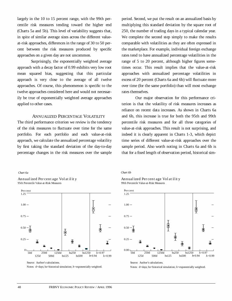
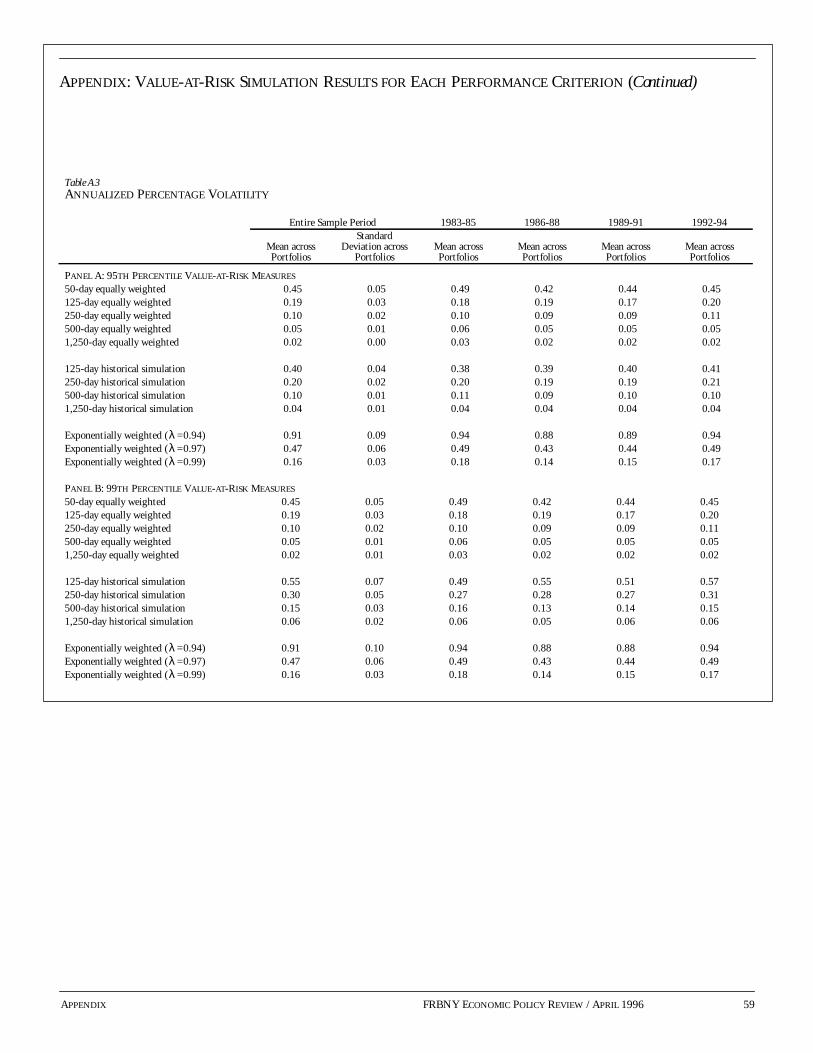
ANNUALIZED PERCENTAGE VOLATILITY
The third performance criterion we review is the tendency
of the risk measures to fluctuate over time for the same
portfolio. For each portfolio and each value-at-risk
approach, we calculate the annualized percentage volatility
by first taking the standard deviation of the day-to-day
percentage changes in the risk measures over the sample
period. Second, we put the result on an annualized basis by
multiplying this standard deviation by the square root of
250, the number of trading days in a typical calendar year.
We complete the second step simply to make the results
comparable with volatilities as they are often expressed in
the marketplace. For example, individual foreign exchange
rates tend to have annualized percentage volatilities in the
range of 5 to 20 percent, although higher figures some-
times occur. This result implies that the value-at-risk
approaches with annualized percentage volatilities in
excess of 20 percent (Charts 6a and 6b) will fluctuate more
over time (for the same portfolio) than will most exchange
rates themselves.
Our major observation for this performance cri-
terion is that the volatility of risk measures increases as
reliance on recent data increases. As shown in Charts 6a
and 6b, this increase is true for both the 95th and 99th
percentile risk measures and for all three categories of
value-at-risk approaches. This result is not surprising, and
indeed it is clearly apparent in Charts 1-3, which depict
time series of different value-at-risk approaches over the
sample period. Also worth noting in Charts 6a and 6b is
that for a fixed length of observation period, historical sim-
FRBNY ECONOMIC POLICY REVIEW / APRIL 1996 49
Chart 7a
Percent
Fraction of Outcomes Covered
95th Percentile Value-at-Risk Measures
50d125d
250d500d
1250d λ�=0.97hs125
hs250hs500
hs1250λ�=0.94 λ�=0.99
50d125d
250d500d
1250d λ�=0.97hs125
hs250hs500
hs1250λ�=0.94 λ�=0.99
Source: Author’�s calculations.
Chart 7b
Percent
Fraction of Outcomes Covered
99th Percentile Value-at-Risk Measures
Source: Author’�s calculations.
0.93
0.94
0.95
0.96
0.97
0.975
0.980
0.985
0.990
0.995
Notes: d=days; hs=historical simulation; λ=exponentially weighted. Notes: d=days; hs=historical simulation; λ=exponentially weighted.
ulation approaches appear to be more variable than the cor-
responding equally weighted moving average approaches.
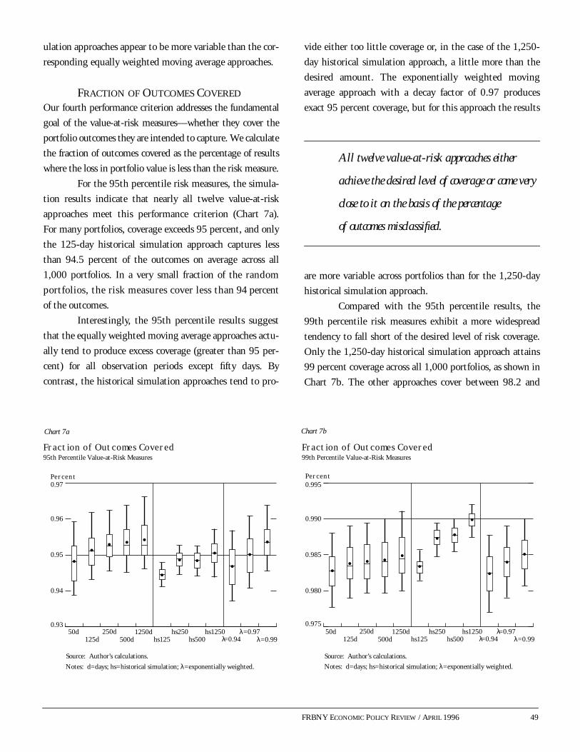
FRACTION OF OUTCOMES COVERED
Our fourth performance criterion addresses the fundamental
goal of the value-at-risk measures—whether they cover the
portfolio outcomes they are intended to capture. We calculate
the fraction of outcomes covered as the percentage of results
where the loss in portfolio value is less than the risk measure.
For the 95th percentile risk measures, the simula-
tion results indicate that nearly all twelve value-at-risk
approaches meet this performance criterion (Chart 7a).
For many portfolios, coverage exceeds 95 percent, and only
the 125-day historical simulation approach captures less
than 94.5 percent of the outcomes on average across all
1,000 portfolios. In a very small fraction of the random
portfolios, the risk measures cover less than 94 percent
of the outcomes.
Interestingly, the 95th percentile results suggest
that the equally weighted moving average approaches actu-
ally tend to produce excess coverage (greater than 95 per-
cent) for all observation periods except fifty days. By
contrast, the historical simulation approaches tend to pro-
vide either too little coverage or, in the case of the 1,250-
day historical simulation approach, a little more than the
desired amount. The exponentially weighted moving
average approach with a decay factor of 0.97 produces
exact 95 percent coverage, but for this approach the results
are more variable across portfolios than for the 1,250-day
historical simulation approach.
Compared with the 95th percentile results, the
99th percentile risk measures exhibit a more widespread
tendency to fall short of the desired level of risk coverage.
Only the 1,250-day historical simulation approach attains
99 percent coverage across all 1,000 portfolios, as shown in
Chart 7b. The other approaches cover between 98.2 and
All twelve value-at-risk approaches either
achieve the desired level of coverage or come very
close to it on the basis of the percentage
of outcomes misclassified.
50 FRBNY ECONOMIC POLICY REVIEW / APRIL 1996
98.8 percent of the outcomes on average across portfolios.
Of course, the consequences of such a shortfall in perfor-
mance depend on the particular circumstances in which
the value-at-risk model is being used. A coverage level of
98.2 percent when a risk manager desires 99 percent
implies that the value-at-risk model misclassifies approxi-
mately two outcomes every year (assuming that there are
250 trading days per calendar year).
Overall, the results in Charts 7a and 7b support
the conclusion that all twelve value-at-risk approaches
either achieve the desired level of coverage or come very
close to it on the basis of the percentage of outcomes mis-
classified. Clearly, the best performer is the 1,250-day his-
torical simulation approach, which attains almost exact
coverage for both the 95th and 99th percentiles, while the
worst performer is the 125-day historical simulation
approach, partly because of its short-term construction.19
One explanation for the superior performance of the 1,250-
day historical simulation is that the unconditional distri-
bution of changes in portfolio value is relatively stable and
that accurate estimates of extreme percentiles require the
use of long periods. These results underscore the problems
associated with the assumption of normality for 99th per-
centiles and are consistent with findings in other recent
studies of value-at-risk models.20
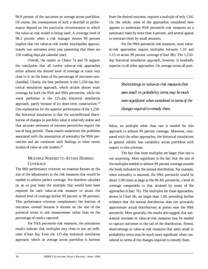
MULTIPLE NEEDED TO ATTAIN DESIRED
COVERAGE
The fifth performance criterion we examine focuses on the
size of the adjustments in the risk measures that would be
needed to achieve perfect coverage. We therefore calculate
on an ex post basis the multiple that would have been
required for each value-at-risk measure to attain the
desired level of coverage (either 95 percent or 99 percent).
This performance criterion complements the fraction of
outcomes covered because it focuses on the size of the
potential errors in risk measurement rather than on the
percentage of results captured.
For 95th percentile risk measures, the simulation
results indicate that multiples very close to one are suffi-
cient (Chart 8a). Even the 125-day historical simulation
approach, which on average across portfolios is furthest
from the desired outcome, requires a multiple of only 1.04.
On the whole, none of the approaches considered here
appears to understate 95th percentile risk measures on a
systematic basis by more than 4 percent, and several appear
to overstate them by small amounts.
For the 99th percentile risk measures, most value-
at-risk approaches require multiples between 1.10 and
1.15 to attain 99 percent coverage (Chart 8b). The 1,250-
day historical simulation approach, however, is markedly
superior to all other approaches. On average across all port-
folios, no multiple other than one is needed for this
approach to achieve 99 percent coverage. Moreover, com-
pared with the other approaches, the historical simulations
in general exhibit less variability across portfolios with
respect to this criterion.
The fact that most multiples are larger than one is
not surprising. More significant is the fact that the size of
the multiples needed to achieve 99 percent coverage exceeds
the levels indicated by the normal distribution. For example,
when normality is assumed, the 99th percentile would be
about 1.08 times as large as the 98.4th percentile, a level of
coverage comparable to that attained by many of the
approaches (Chart 7b). The multiples for these approaches,
shown in Chart 8b, are larger than 1.08, providing further
evidence that the normal distribution does not accurately
approximate actual distributions at points near the 99th
percentile. More generally, the results also suggest that sub-
stantial increases in value-at-risk measures may be needed
to capture outcomes in the tail of the distribution. Hence,
shortcomings in value-at-risk measures that seem small in
probability terms may be much more significant when con-
sidered in terms of the changes required to remedy them.
Shortcomings in value-at-risk measures that
seem small in probability terms may be much
more significant when considered in terms of the
changes required to remedy them.
FRBNY ECONOMIC POLICY REVIEW / APRIL 1996 51
Chart 8a
Multiple
Multiple Needed to Attain 95 Percent Coverage
95th Percentile Value-at-Risk Measures
50d125d
250d500d
1250d λ�=0.97hs125
hs250hs500
hs1250λ�=0.94 λ�=0.99
50d125d
250d500d
1250d λ�=0.97hs125
hs250hs500
hs1250λ�=0.94 λ�=0.99
Source: Author’�s calculations.
Chart 8b
Multiple
Multiple Needed to Attain 99 Percent Coverage
99th Percentile Value-at-Risk Measures
Source: Author’�s calculations.
0.8
0.9
1.0
1.1
1.2
0.9
1.0
1.1
1.2
1.3
Notes: d=days; hs=historical simulation; λ=exponentially weighted. Notes: d=days; hs=historical simulation; λ=exponentially weighted.
These results lead to an important question: what
distributional assumptions other than normality can be
used when constructing value-at-risk measures using a
variance-covariance approach? The t-distribution is often
cited as a good candidate, because extreme outcomes occur
more often under t-distributions than under the normal
distribution.21 A brief analysis shows that the use of a
t-distribution for the 99th percentile has some merit.
To calculate a value-at-risk measure for a single
percentile assuming the t-distribution, the value-at-risk
measure calculated with the assumption of normality is
multiplied by a fixed multiple. As the results in Chart 8b
suggest, fixed multiples between 1.10 and 1.15 are appro-
priate for the variance-covariance approaches. It follows
that t-distributions with between four and six degrees of
freedom are appropriate for the 99th percentile risk mea-
sures.22 The use of these particular t-distributions, how-
ever, would lead to substantial overestimation of 95th
percentile risk measures because the actual distributions
near the 95th percentile are much closer to normality.
Since the use of t-distributions for risk measurement
involves a scaling up of the risk measures that are calcu-
lated assuming normality, the distributions are likely to be
useful, although they may be more helpful for some per-
centiles than for others.
AVERAGE MULTIPLE OF TAIL EVENT
TO RISK MEASURE
The sixth performance criterion that we review relates to
the size of outcomes not covered by the risk measures.23To
address these outcomes, we measure the degree to which
events in the tail of the distribution typically exceed the
value-at-risk measure by calculating the average multiple
of these outcomes (“tail events”) to their corresponding
value-at-risk measures.
Tail events are defined as the largest percentage
of losses measured relative to the respective value-at-risk
estimate—the largest 5 percent in the case of 95th per-
centile risk measures and the largest 1 percent in the case
of 99th percentile risk measures. For example, if the
value-at-risk measure is $1.5 million and the actual port-
folio outcome is a loss of $3 million, the size of the loss
relative to the risk measure would be two. Note that this
definition implies that the tail events for one value-at-
risk approach may not be the same as those for another
approach, even for the same portfolio, because the risk
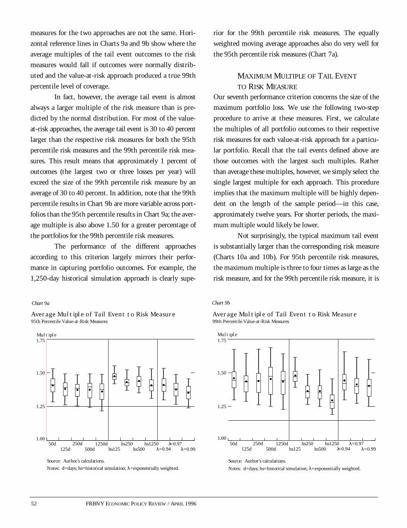
52 FRBNY ECONOMIC POLICY REVIEW / APRIL 1996
Chart 9a
Multiple
Average Multiple of Tail Event to Risk Measure
95th Percentile Value-at-Risk Measures
50d125d
250d500d
1250d λ�=0.97hs125
hs250hs500
hs1250λ�=0.94 λ�=0.99
50d125d
250d500d
1250d λ�=0.97hs125
hs250hs500
hs1250λ�=0.94 λ�=0.99
Source: Author’�s calculations.
Chart 9b
Multiple
Average Multiple of Tail Event to Risk Measure
99th Percentile Value-at-Risk Measures
Source: Author’�s calculations.
1.00
1.25
1.50
1.75
1.00
1.25
1.50
1.75
Notes: d=days; hs=historical simulation; λ=exponentially weighted. Notes: d=days; hs=historical simulation; λ=exponentially weighted.
measures for the two approaches are not the same. Hori-
zontal reference lines in Charts 9a and 9b show where the
average multiples of the tail event outcomes to the risk
measures would fall if outcomes were normally distrib-
uted and the value-at-risk approach produced a true 99th
percentile level of coverage.
In fact, however, the average tail event is almost
always a larger multiple of the risk measure than is pre-
dicted by the normal distribution. For most of the value-
at-risk approaches, the average tail event is 30 to 40 percent
larger than the respective risk measures for both the 95th
percentile risk measures and the 99th percentile risk mea-
sures. This result means that approximately 1 percent of
outcomes (the largest two or three losses per year) will
exceed the size of the 99th percentile risk measure by an
average of 30 to 40 percent. In addition, note that the 99th
percentile results in Chart 9b are more variable across port-
folios than the 95th percentile results in Chart 9a; the aver-
age multiple is also above 1.50 for a greater percentage of
the portfolios for the 99th percentile risk measures.
The performance of the different approaches
according to this criterion largely mirrors their perfor-
mance in capturing portfolio outcomes. For example, the
1,250-day historical simulation approach is clearly supe-
rior for the 99th percentile risk measures. The equally
weighted moving average approaches also do very well for
the 95th percentile risk measures (Chart 7a).
MAXIMUM MULTIPLE OF TAIL EVENT
TO RISK MEASURE
Our seventh performance criterion concerns the size of the
maximum portfolio loss. We use the following two-step
procedure to arrive at these measures. First, we calculate
the multiples of all portfolio outcomes to their respective
risk measures for each value-at-risk approach for a particu-
lar portfolio. Recall that the tail events defined above are
those outcomes with the largest such multiples. Rather
than average these multiples, however, we simply select the
single largest multiple for each approach. This procedure
implies that the maximum multiple will be highly depen-
dent on the length of the sample period—in this case,
approximately twelve years. For shorter periods, the maxi-
mum multiple would likely be lower.
Not surprisingly, the typical maximum tail event
is substantially larger than the corresponding risk measure
(Charts 10a and 10b). For 95th percentile risk measures,
the maximum multiple is three to four times as large as the
risk measure, and for the 99th percentile risk measure, it is
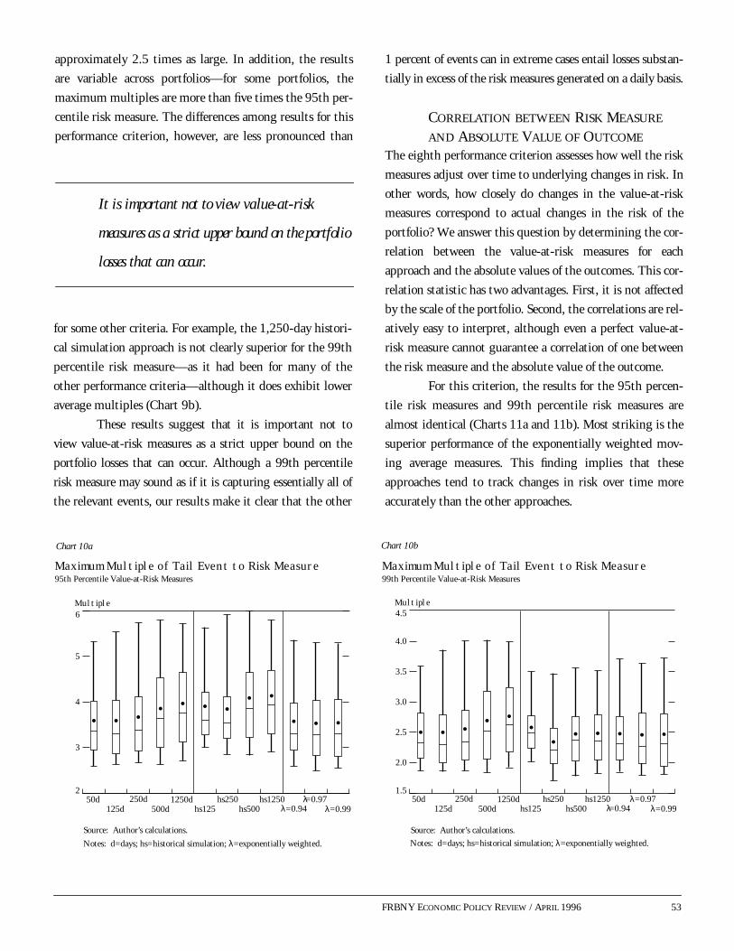
FRBNY ECONOMIC POLICY REVIEW / APRIL 1996 53
Chart 10a
Multiple
Maximum Multiple of Tail Event to Risk Measure
95th Percentile Value-at-Risk Measures
50d125d
250d500d
1250d λ�=0.97hs125
hs250hs500
hs1250λ�=0.94 λ�=0.99
50d125d
250d500d
1250d λ�=0.97hs125
hs250hs500
hs1250λ�=0.94 λ�=0.99
Source: Author’�s calculations.
Chart 10b
Multiple
Maximum Multiple of Tail Event to Risk Measure
99th Percentile Value-at-Risk Measures
Source: Author’�s calculations.
2
3
4
5
6
1.5
2.0
2.5
3.0
3.5
4.0
4.5
Notes: d=days; hs=historical simulation; λ=exponentially weighted. Notes: d=days; hs=historical simulation; λ=exponentially weighted.
approximately 2.5 times as large. In addition, the results
are variable across portfolios—for some portfolios, the
maximum multiples are more than five times the 95th per-
centile risk measure. The differences among results for this
performance criterion, however, are less pronounced than
for some other criteria. For example, the 1,250-day histori-
cal simulation approach is not clearly superior for the 99th
percentile risk measure—as it had been for many of the
other performance criteria—although it does exhibit lower
average multiples (Chart 9b).
These results suggest that it is important not to
view value-at-risk measures as a strict upper bound on the
portfolio losses that can occur. Although a 99th percentile
risk measure may sound as if it is capturing essentially all of
the relevant events, our results make it clear that the other
1 percent of events can in extreme cases entail losses substan-
tially in excess of the risk measures generated on a daily basis.
CORRELATION BETWEEN RISK MEASURE
AND ABSOLUTE VALUE OF OUTCOME
The eighth performance criterion assesses how well the risk
measures adjust over time to underlying changes in risk. In
other words, how closely do changes in the value-at-risk
measures correspond to actual changes in the risk of the
portfolio? We answer this question by determining the cor-
relation between the value-at-risk measures for each
approach and the absolute values of the outcomes. This cor-
relation statistic has two advantages. First, it is not affected
by the scale of the portfolio. Second, the correlations are rel-
atively easy to interpret, although even a perfect value-at-
risk measure cannot guarantee a correlation of one between
the risk measure and the absolute value of the outcome.
For this criterion, the results for the 95th percen-
tile risk measures and 99th percentile risk measures are
almost identical (Charts 11a and 11b). Most striking is the
superior performance of the exponentially weighted mov-
ing average measures. This finding implies that these
approaches tend to track changes in risk over time more
accurately than the other approaches.
It is important not to view value-at-risk
measures as a strict upper bound on the portfolio
losses that can occur.

54 FRBNY ECONOMIC POLICY REVIEW / APRIL 1996
Chart 11a
Percent
Correlation between Risk Measure and Absolute
Value of Outcome
95th Percentile Value-at-Risk Measures
50d125d
250d500d
1250d λ�=0.97hs125
hs250hs500
hs1250λ�=0.94 λ�=0.99
50d125d
250d500d
1250d λ�=0.97hs125
hs250hs500
hs1250λ�=0.94 λ�=0.99
Source: Author’�s calculations.
Chart 11b
Percent
Correlation between Risk Measure and Absolute
Value of Outcome
99th Percentile Value-at-Risk Measures
Source: Author’�s calculations.
-0.1
0
0.1
0.2
0.3
0.4
-0.1
0
0.1
0.2
0.3
0.4
Notes: d=days; hs=historical simulation; λ=exponentially weighted. Notes: d=days; hs=historical simulation; λ=exponentially weighted.
In contrast to the results for mean relative bias
(Charts 4a and 4b) and the fraction of outcomes covered
(Charts 7a and 7b), the results for this performance crite-
rion show that the length of the observation period is
inversely related to performance. Thus, shorter observation
periods tend to lead to higher measures of correlation
between the absolute values of the outcomes and the value-
at-risk measures. This inverse relationship supports the
view that, because market behavior changes over time,
emphasis on recent information can be helpful in tracking
changes in risk.
At the other extreme, the risk measures for the
1,250-day historical simulation approach are essentially
uncorrelated with the absolute values of the outcomes.
Although superior according to other performance criteria,
the 1,250-day results here indicate that this approach reveals
little about actual changes in portfolio risk over time.
MEAN RELATIVE BIAS FOR RISK MEASURES
SCALED TO DESIRED LEVEL OF COVERAGE
The last performance criterion we examine is the mean rel-
ative bias that results when risk measures are scaled to
either 95 percent or 99 percent coverage. Such scaling is
accomplished on an ex post basis by multiplying the risk
measures for each approach by the multiples needed to
attain either exactly 95 percent or exactly 99 percent cover-
age (Charts 8a and 8b). These scaled risk measures provide
the precise amount of coverage desired for each portfolio.
Of course, the scaling for each value-at-risk approach
would not be the same for different portfolios.
Once we have arrived at the scaled value-at-risk
measures, we compare their relative average sizes by using
the mean relative bias calculation, which compares the
average size of the risk measures for each approach to the
average size across all twelve approaches (Charts 4a and
4b). In this case, however, the value-at-risk measures have
been scaled to the desired levels of coverage. The purpose
of this criterion is to determine which approach, once suit-
Because market behavior changes over time,
emphasis on recent information can be helpful in
tracking changes in risk.
FRBNY ECONOMIC POLICY REVIEW / APRIL 1996 55
Chart 12a
Percent
Mean Relative Bias for Risk Measures Scaled to
Cover Exactly 95 Percent
95th Percentile Value-at-Risk Measures
50d125d
250d500d
1250d λ�=0.97hs125
hs250hs500
hs1250λ�=0.94 λ�=0.99
50d125d
250d500d
1250d λ�=0.97hs125
hs250hs500
hs1250λ�=0.94 λ�=0.99
Source: Author’�s calculations.
Chart 12b
Percent
Mean Relative Bias for Risk Measures Scaled to
Cover Exactly 99 Percent
99th Percentile Value-at-Risk Measures
Source: Author’�s calculations.
-0.10
-0.05
0
0.05
0.10
-0.10
-0.05
0
0.05
0.10
Notes: d=days; hs=historical simulation; λ=exponentially weighted. Notes: d=days; hs=historical simulation; λ=exponentially weighted.
ably scaled, could provide the desired level of coverage
with the smallest average risk measures. This performance
criterion also addresses the issue of tracking changes in
portfolio risk—the most efficient approach will be the one
that tracks changes in risk best. In contrast to the correla-
tion statistic discussed in the previous section, however,
this criterion focuses specifically on the 95th and 99th
percentiles.
Once again, the exponentially weighted moving
average approaches appear superior (Charts 12a and 12b).
In particular, the exponentially weighted average approach
with a decay factor of 0.97 appears to perform extremely
well for both 95th and 99th percentile risk measures.
Indeed, for the 99th percentile, it achieves exact 99 percent
coverage with an average size that is 4 percent smaller than
the average of all twelve scaled value-at-risk approaches.
The performance of the other approaches is similar
to that observed for the correlation statistic (Charts 11a
and 11b), but in this case the relationship between effi-
ciency and the length of the observation period is not as
pronounced. In particular, the 50-day equally weighted
approach is somewhat inferior to the 250-day equally
weighted approach—a finding contrary to what is observed
in Charts 11a and 11b—and may reflect the greater influ-
ence of measurement error on short observation periods
along this performance criterion.
At least two caveats apply to these results. First,
they would be difficult to duplicate in practice because the
scaling must be done in advance of the outcomes rather
than ex post. Second, the differences in the average sizes of
the scaled risk measures are simply not very large. Never-
theless, the results suggest that exponentially weighted
average approaches might be capable of providing desired
levels of coverage in an efficient fashion, although they
would need to be scaled up.
CONCLUSIONS
A historical examination of twelve approaches to value-at-
risk modeling shows that in almost all cases the approaches
cover the risk that they are intended to cover. In addition,
the twelve approaches tend to produce risk estimates that
do not differ greatly in average size, although historical
simulation approaches yield somewhat larger 99th percen-
tile risk measures than the variance-covariance approaches.
Despite the similarity in the average size of the
risk estimates, our investigation reveals differences, some-
56 FRBNY ECONOMIC POLICY REVIEW / APRIL 1996
times substantial, among the various value-at-risk
approaches for the same portfolio on the same date. In
terms of variability over time, the value-at-risk approaches
using longer observation periods tend to produce less vari-
able results than those using short observation periods or
weighting recent observations more heavily.
Virtually all of the approaches produce accurate
95th percentile risk measures. The 99th percentile risk
measures, however, are somewhat less reliable and gener-
ally cover only between 98.2 percent and 98.5 percent of
the outcomes. On the one hand, these deficiencies are small
when considered on the basis of the percentage of outcomes
misclassified. On the other hand, the risk measures would
generally need to be increased across the board by 10 per-
cent or more to cover precisely 99 percent of the outcomes.
Interestingly, one exception is the 1,250-day historical
simulation approach, which provides very accurate cover-
age for both 95th and 99th percentile risk measures.
The outcomes that are not covered are typically 30
to 40 percent larger than the risk measures and are also
larger than predicted by the normal distribution. In some
cases, daily losses over the twelve-year sample period are
several times larger than the corresponding value-at-risk
measures. These examples make it clear that value-at-risk
measures—even at the 99th percentile—do not “bound”
possible losses.
Also clear is the difficulty of anticipating or tracking
changes in risk over time. For this performance criterion, the
exponentially weighted moving average approaches appear to
be superior. If it were possible to scale all approaches ex post to
achieve the desired level of coverage over the sample period,
these approaches would produce the smallest scaled risk
measures.
What more general conclusions can be drawn
from these results? In many respects, the simulation esti-
mates clearly reflect two well-known characteristics of
daily financial market data. First, extreme outcomes occur
more often and are larger than predicted by the normal
distribution (fat tails). Second, the size of market move-
ments is not constant over time (conditional volatility).
Clearly, constructing value-at-risk models that perform
well by every measure is a difficult task. Thus, although
we cannot recommend any single value-at-risk approach,
our results suggest that further research aimed at combin-
ing the best features of the approaches examined here may
be worthwhile.
APPENDIX: VALUE-AT-RISK SIMULATION RESULTS FOR EACH PERFORMANCE CRITERION
APPENDIX FRBNY ECONOMIC POLICY REVIEW / APRIL 1996 57
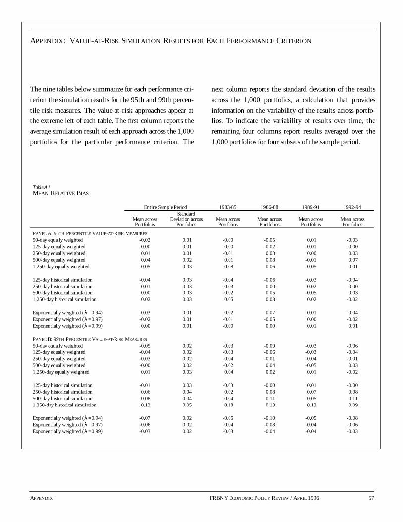
The nine tables below summarize for each performance cri-
terion the simulation results for the 95th and 99th percen-
tile risk measures. The value-at-risk approaches appear at
the extreme left of each table. The first column reports the
average simulation result of each approach across the 1,000
portfolios for the particular performance criterion. The
next column reports the standard deviation of the results
across the 1,000 portfolios, a calculation that provides
information on the variability of the results across portfo-
lios. To indicate the variability of results over time, the
remaining four columns report results averaged over the
1,000 portfolios for four subsets of the sample period.
Table A1MEAN RELATIVE BIAS
Entire Sample Period 1983-85 1986-88 1989-91 1992-94
Mean acrossPortfolios
StandardDeviation across
PortfoliosMean acrossPortfolios
Mean acrossPortfolios
Mean acrossPortfolios
Mean acrossPortfolios
PANEL A: 95TH PERCENTILE VALUE-AT-RISK MEASURES
50-day equally weighted -0.02 0.01 -0.00 -0.05 0.01 -0.03125-day equally weighted -0.00 0.01 -0.00 -0.02 0.01 -0.00250-day equally weighted 0.01 0.01 -0.01 0.03 0.00 0.03500-day equally weighted 0.04 0.02 0.01 0.08 -0.01 0.071,250-day equally weighted 0.05 0.03 0.08 0.06 0.05 0.01
125-day historical simulation -0.04 0.03 -0.04 -0.06 -0.03 -0.04250-day historical simulation -0.01 0.03 -0.03 0.00 -0.02 0.00500-day historical simulation 0.00 0.03 -0.02 0.05 -0.05 0.031,250-day historical simulation 0.02 0.03 0.05 0.03 0.02 -0.02
Exponentially weighted ( =0.94) -0.03 0.01 -0.02 -0.07 -0.01 -0.04Exponentially weighted ( =0.97) -0.02 0.01 -0.01 -0.05 0.00 -0.02Exponentially weighted ( =0.99) 0.00 0.01 -0.00 0.00 0.01 0.01
PANEL B: 99TH PERCENTILE VALUE-AT-RISK MEASURES
50-day equally weighted -0.05 0.02 -0.03 -0.09 -0.03 -0.06125-day equally weighted -0.04 0.02 -0.03 -0.06 -0.03 -0.04250-day equally weighted -0.03 0.02 -0.04 -0.01 -0.04 -0.01500-day equally weighted -0.00 0.02 -0.02 0.04 -0.05 0.031,250-day equally weighted 0.01 0.03 0.04 0.02 0.01 -0.02
125-day historical simulation -0.01 0.03 -0.03 -0.00 0.01 -0.00250-day historical simulation 0.06 0.04 0.02 0.08 0.07 0.08500-day historical simulation 0.08 0.04 0.04 0.11 0.05 0.111,250-day historical simulation 0.13 0.05 0.18 0.13 0.13 0.09
Exponentially weighted ( =0.94) -0.07 0.02 -0.05 -0.10 -0.05 -0.08Exponentially weighted ( =0.97) -0.06 0.02 -0.04 -0.08 -0.04 -0.06Exponentially weighted ( =0.99) -0.03 0.02 -0.03 -0.04 -0.04 -0.03
λλλ
λλλ

58 FRBNY ECONOMIC POLICY REVIEW / APRIL 1996 APPENDIX
APPENDIX: VALUE-AT-RISK SIMULATION RESULTS FOR EACH PERFORMANCE CRITERION (Continued)
Table A2ROOT MEAN SQUARED RELATIVE BIAS
Entire Sample Period 1983-85 1986-88 1989-91 1992-94
Mean acrossPortfolios
StandardDeviation across
PortfoliosMean acrossPortfolios
Mean acrossPortfolios
Mean acrossPortfolios
Mean acrossPortfolios
PANEL A: 95TH PERCENTILE VALUE-AT-RISK MEASURES
50-day equally weighted 0.16 0.01 0.17 0.15 0.14 0.16125-day equally weighted 0.10 0.01 0.10 0.10 0.08 0.11250-day equally weighted 0.09 0.01 0.08 0.09 0.08 0.09500-day equally weighted 0.13 0.02 0.13 0.13 0.08 0.131,250-day equally weighted 0.16 0.04 0.18 0.14 0.14 0.14
125-day historical simulation 0.14 0.02 0.15 0.13 0.13 0.14250-day historical simulation 0.11 0.01 0.12 0.11 0.10 0.11500-day historical simulation 0.13 0.02 0.14 0.13 0.10 0.141,250-day historical simulation 0.15 0.03 0.17 0.13 0.13 0.15
Exponentially weighted ( =0.94) 0.18 0.01 0.20 0.17 0.17 0.19Exponentially weighted ( =0.97) 0.12 0.01 0.13 0.11 0.10 0.13Exponentially weighted ( =0.99) 0.05 0.01 0.05 0.04 0.04 0.05
PANEL B: 99TH PERCENTILE VALUE-AT-RISK MEASURES
50-day equally weighted 0.16 0.01 0.17 0.16 0.14 0.16125-day equally weighted 0.10 0.01 0.11 0.11 0.08 0.11250-day equally weighted 0.09 0.01 0.09 0.09 0.09 0.09500-day equally weighted 0.12 0.02 0.13 0.12 0.10 0.121,250-day equally weighted 0.14 0.03 0.16 0.13 0.13 0.14
125-day historical simulation 0.18 0.03 0.15 0.19 0.17 0.17250-day historical simulation 0.16 0.03 0.14 0.15 0.16 0.16500-day historical simulation 0.16 0.04 0.15 0.18 0.12 0.171,250-day historical simulation 0.22 0.06 0.24 0.20 0.19 0.19
Exponentially weighted ( =0.94) 0.19 0.01 0.20 0.19 0.17 0.19Exponentially weighted ( =0.97) 0.13 0.01 0.14 0.13 0.11 0.13Exponentially weighted ( =0.99) 0.06 0.01 0.06 0.06 0.05 0.06
λλλ
λλλ
APPENDIX: VALUE-AT-RISK SIMULATION RESULTS FOR EACH PERFORMANCE CRITERION (Continued)
APPENDIX FRBNY ECONOMIC POLICY REVIEW / APRIL 1996 59
Table A3ANNUALIZED PERCENTAGE VOLATILITY
Entire Sample Period 1983-85 1986-88 1989-91 1992-94
Mean acrossPortfolios
StandardDeviation across
PortfoliosMean acrossPortfolios
Mean acrossPortfolios
Mean acrossPortfolios
Mean acrossPortfolios
PANEL A: 95TH PERCENTILE VALUE-AT-RISK MEASURES
50-day equally weighted 0.45 0.05 0.49 0.42 0.44 0.45125-day equally weighted 0.19 0.03 0.18 0.19 0.17 0.20250-day equally weighted 0.10 0.02 0.10 0.09 0.09 0.11500-day equally weighted 0.05 0.01 0.06 0.05 0.05 0.051,250-day equally weighted 0.02 0.00 0.03 0.02 0.02 0.02
125-day historical simulation 0.40 0.04 0.38 0.39 0.40 0.41250-day historical simulation 0.20 0.02 0.20 0.19 0.19 0.21500-day historical simulation 0.10 0.01 0.11 0.09 0.10 0.101,250-day historical simulation 0.04 0.01 0.04 0.04 0.04 0.04
Exponentially weighted ( =0.94) 0.91 0.09 0.94 0.88 0.89 0.94Exponentially weighted ( =0.97) 0.47 0.06 0.49 0.43 0.44 0.49Exponentially weighted ( =0.99) 0.16 0.03 0.18 0.14 0.15 0.17
PANEL B: 99TH PERCENTILE VALUE-AT-RISK MEASURES
50-day equally weighted 0.45 0.05 0.49 0.42 0.44 0.45125-day equally weighted 0.19 0.03 0.18 0.19 0.17 0.20250-day equally weighted 0.10 0.02 0.10 0.09 0.09 0.11500-day equally weighted 0.05 0.01 0.06 0.05 0.05 0.051,250-day equally weighted 0.02 0.01 0.03 0.02 0.02 0.02
125-day historical simulation 0.55 0.07 0.49 0.55 0.51 0.57250-day historical simulation 0.30 0.05 0.27 0.28 0.27 0.31500-day historical simulation 0.15 0.03 0.16 0.13 0.14 0.151,250-day historical simulation 0.06 0.02 0.06 0.05 0.06 0.06
Exponentially weighted ( =0.94) 0.91 0.10 0.94 0.88 0.88 0.94Exponentially weighted ( =0.97) 0.47 0.06 0.49 0.43 0.44 0.49Exponentially weighted ( =0.99) 0.16 0.03 0.18 0.14 0.15 0.17
λλλ
λλλ

60 FRBNY ECONOMIC POLICY REVIEW / APRIL 1996 APPENDIX
APPENDIX: VALUE-AT-RISK SIMULATION RESULTS FOR EACH PERFORMANCE CRITERION (Continued)
Table A4FRACTION OF OUTCOMES COVERED
Entire Sample Period 1983-85 1986-88 1989-91 1992-94
Mean acrossPortfolios
StandardDeviation across
PortfoliosMean acrossPortfolios
Mean acrossPortfolios
Mean acrossPortfolios
Mean acrossPortfolios
PANEL A: 95TH PERCENTILE VALUE-AT-RISK MEASURES
50-day equally weighted 0.948 0.006 0.948 0.947 0.949 0.948125-day equally weighted 0.951 0.006 0.950 0.953 0.951 0.953250-day equally weighted 0.953 0.005 0.946 0.960 0.950 0.956500-day equally weighted 0.954 0.006 0.946 0.963 0.947 0.9581,250-day equally weighted 0.954 0.006 0.954 0.959 0.954 0.950
125-day historical simulation 0.944 0.002 0.943 0.946 0.943 0.946250-day historical simulation 0.949 0.003 0.943 0.955 0.945 0.952500-day historical simulation 0.948 0.003 0.942 0.959 0.941 0.9521,250-day historical simulation 0.951 0.004 0.951 0.956 0.951 0.945
Exponentially weighted ( =0.94) 0.947 0.006 0.948 0.946 0.947 0.946Exponentially weighted ( =0.97) 0.950 0.006 0.950 0.950 0.950 0.950Exponentially weighted ( =0.99) 0.954 0.006 0.950 0.957 0.951 0.956
PANEL B: 99TH PERCENTILE VALUE-AT-RISK MEASURES
50-day equally weighted 0.983 0.003 0.985 0.982 0.982 0.983125-day equally weighted 0.984 0.003 0.984 0.984 0.982 0.984250-day equally weighted 0.984 0.003 0.982 0.987 0.982 0.986500-day equally weighted 0.984 0.003 0.981 0.989 0.981 0.9871,250-day equally weighted 0.985 0.003 0.984 0.988 0.984 0.983
125-day historical simulation 0.983 0.001 0.983 0.985 0.982 0.984250-day historical simulation 0.987 0.001 0.984 0.991 0.986 0.989500-day historical simulation 0.988 0.001 0.985 0.991 0.986 0.9901,250-day historical simulation 0.990 0.001 0.990 0.992 0.989 0.989
Exponentially weighted ( =0.94) 0.982 0.003 0.984 0.981 0.982 0.983Exponentially weighted ( =0.97) 0.984 0.003 0.986 0.983 0.983 0.984Exponentially weighted ( =0.99) 0.985 0.003 0.985 0.986 0.983 0.986
λλλ
λλλ

APPENDIX: VALUE-AT-RISK SIMULATION RESULTS FOR EACH PERFORMANCE CRITERION (Continued)
APPENDIX FRBNY ECONOMIC POLICY REVIEW / APRIL 1996 61
Table A5MULTIPLE NEEDED TO ATTAIN DESIRED COVERAGE LEVEL
Entire Sample Period 1983-85 1986-88 1989-91 1992-94
Mean acrossPortfolios
StandardDeviation across
PortfoliosMean acrossPortfolios
Mean acrossPortfolios
Mean acrossPortfolios
Mean acrossPortfolios
PANEL A: 95TH PERCENTILE VALUE-AT-RISK MEASURES
50-day equally weighted 1.01 0.05 1.01 1.02 1.01 1.02125-day equally weighted 0.99 0.04 1.00 0.98 0.99 0.98250-day equally weighted 0.98 0.04 1.02 0.93 1.00 0.95500-day equally weighted 0.97 0.04 1.02 0.90 1.02 0.931,250-day equally weighted 0.97 0.05 0.95 0.93 0.97 1.00
125-day historical simulation 1.04 0.01 1.05 1.03 1.05 1.03250-day historical simulation 1.01 0.02 1.05 0.96 1.03 0.98500-day historical simulation 1.01 0.02 1.06 0.94 1.06 0.991,250-day historical simulation 1.00 0.03 0.98 0.95 0.99 1.04
Exponentially weighted ( =0.94) 1.02 0.05 1.01 1.03 1.02 1.03Exponentially weighted ( =0.97) 1.00 0.04 0.99 1.00 1.00 1.00Exponentially weighted ( =0.99) 0.97 0.04 0.99 0.95 0.99 0.96
PANEL B: 99TH PERCENTILE VALUE-AT-RISK MEASURES
50-day equally weighted 1.15 0.06 1.11 1.19 1.19 1.14125-day equally weighted 1.13 0.07 1.12 1.11 1.17 1.13250-day equally weighted 1.13 0.07 1.17 1.06 1.20 1.11500-day equally weighted 1.13 0.08 1.22 1.03 1.20 1.101,250-day equally weighted 1.11 0.08 1.12 1.04 1.13 1.17
125-day historical simulation 1.14 0.03 1.15 1.13 1.18 1.16250-day historical simulation 1.06 0.03 1.11 0.99 1.12 1.04500-day historical simulation 1.05 0.03 1.13 0.98 1.10 1.021,250-day historical simulation 1.00 0.04 1.00 0.94 1.01 1.04
Exponentially weighted ( =0.94) 1.14 0.06 1.12 1.19 1.14 1.16Exponentially weighted ( =0.97) 1.12 0.06 1.09 1.15 1.15 1.12Exponentially weighted ( =0.99) 1.10 0.06 1.11 1.08 1.17 1.09
λλλ
λλλ

62 FRBNY ECONOMIC POLICY REVIEW / APRIL 1996 APPENDIX
APPENDIX: VALUE-AT-RISK SIMULATION RESULTS FOR EACH PERFORMANCE CRITERION (Continued)
Table A6AVERAGE MULTIPLE OF TAIL EVENT TO RISK MEASURE
Entire Sample Period 1983-85 1986-88 1989-91 1992-94
Mean acrossPortfolios
StandardDeviation across
PortfoliosMean acrossPortfolios
Mean acrossPortfolios
Mean acrossPortfolios
Mean acrossPortfolios
PANEL A: 95TH PERCENTILE VALUE-AT-RISK MEASURES
50-day equally weighted 1.41 0.07 1.40 1.41 1.41 1.41125-day equally weighted 1.38 0.07 1.39 1.35 1.39 1.39250-day equally weighted 1.37 0.07 1.43 1.28 1.41 1.36500-day equally weighted 1.38 0.08 1.46 1.24 1.43 1.341,250-day equally weighted 1.36 0.08 1.35 1.27 1.35 1.43
125-day historical simulation 1.48 0.04 1.47 1.45 1.49 1.50250-day historical simulation 1.43 0.05 1.49 1.34 1.46 1.44500-day historical simulation 1.44 0.06 1.53 1.29 1.48 1.431,250-day historical simulation 1.41 0.07 1.39 1.31 1.39 1.50
Exponentially weighted ( =0.94) 1.41 0.07 1.39 1.42 1.41 1.42Exponentially weighted ( =0.97) 1.38 0.07 1.37 1.38 1.38 1.38Exponentially weighted ( =0.99) 1.35 0.07 1.38 1.30 1.38 1.34
PANEL B: 99TH PERCENTILE VALUE-AT-RISK MEASURES
50-day equally weighted 1.46 0.12 1.48 1.45 1.48 1.47125-day equally weighted 1.44 0.11 1.45 1.41 1.42 1.50250-day equally weighted 1.44 0.13 1.49 1.34 1.44 1.50500-day equally weighted 1.46 0.14 1.56 1.29 1.46 1.471,250-day equally weighted 1.44 0.14 1.43 1.31 1.39 1.55
125-day historical simulation 1.48 0.07 1.51 1.47 1.46 1.55250-day historical simulation 1.37 0.07 1.44 1.28 1.37 1.41500-day historical simulation 1.37 0.09 1.46 1.25 1.34 1.401,250-day historical simulation 1.30 0.10 1.28 1.20 1.25 1.40
Exponentially weighted ( =0.94) 1.44 0.11 1.45 1.44 1.44 1.48Exponentially weighted ( =0.97) 1.42 0.11 1.43 1.40 1.41 1.45Exponentially weighted ( =0.99) 1.40 0.11 1.44 1.35 1.42 1.44
λλλ
λλλ
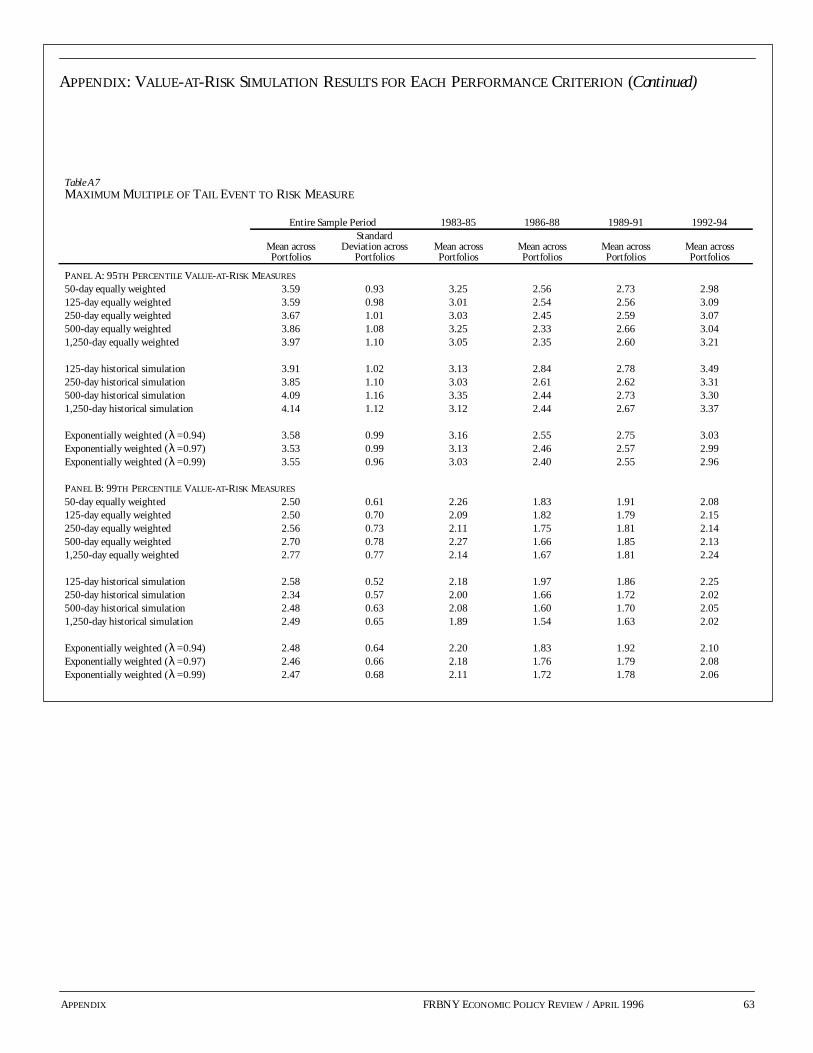
APPENDIX: VALUE-AT-RISK SIMULATION RESULTS FOR EACH PERFORMANCE CRITERION (Continued)
APPENDIX FRBNY ECONOMIC POLICY REVIEW / APRIL 1996 63
Table A7MAXIMUM MULTIPLE OF TAIL EVENT TO RISK MEASURE
Entire Sample Period 1983-85 1986-88 1989-91 1992-94
Mean acrossPortfolios
StandardDeviation across
PortfoliosMean acrossPortfolios
Mean acrossPortfolios
Mean acrossPortfolios
Mean acrossPortfolios
PANEL A: 95TH PERCENTILE VALUE-AT-RISK MEASURES
50-day equally weighted 3.59 0.93 3.25 2.56 2.73 2.98125-day equally weighted 3.59 0.98 3.01 2.54 2.56 3.09250-day equally weighted 3.67 1.01 3.03 2.45 2.59 3.07500-day equally weighted 3.86 1.08 3.25 2.33 2.66 3.041,250-day equally weighted 3.97 1.10 3.05 2.35 2.60 3.21
125-day historical simulation 3.91 1.02 3.13 2.84 2.78 3.49250-day historical simulation 3.85 1.10 3.03 2.61 2.62 3.31500-day historical simulation 4.09 1.16 3.35 2.44 2.73 3.301,250-day historical simulation 4.14 1.12 3.12 2.44 2.67 3.37
Exponentially weighted ( =0.94) 3.58 0.99 3.16 2.55 2.75 3.03Exponentially weighted ( =0.97) 3.53 0.99 3.13 2.46 2.57 2.99Exponentially weighted ( =0.99) 3.55 0.96 3.03 2.40 2.55 2.96
PANEL B: 99TH PERCENTILE VALUE-AT-RISK MEASURES
50-day equally weighted 2.50 0.61 2.26 1.83 1.91 2.08125-day equally weighted 2.50 0.70 2.09 1.82 1.79 2.15250-day equally weighted 2.56 0.73 2.11 1.75 1.81 2.14500-day equally weighted 2.70 0.78 2.27 1.66 1.85 2.131,250-day equally weighted 2.77 0.77 2.14 1.67 1.81 2.24
125-day historical simulation 2.58 0.52 2.18 1.97 1.86 2.25250-day historical simulation 2.34 0.57 2.00 1.66 1.72 2.02500-day historical simulation 2.48 0.63 2.08 1.60 1.70 2.051,250-day historical simulation 2.49 0.65 1.89 1.54 1.63 2.02
Exponentially weighted ( =0.94) 2.48 0.64 2.20 1.83 1.92 2.10Exponentially weighted ( =0.97) 2.46 0.66 2.18 1.76 1.79 2.08Exponentially weighted ( =0.99) 2.47 0.68 2.11 1.72 1.78 2.06
λλλ
λλλ
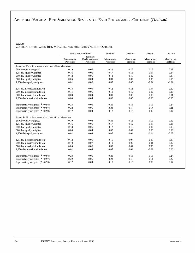
64 FRBNY ECONOMIC POLICY REVIEW / APRIL 1996 APPENDIX
APPENDIX: VALUE-AT-RISK SIMULATION RESULTS FOR EACH PERFORMANCE CRITERION (Continued)
Table A8CORRELATION BETWEEN RISK MEASURES AND ABSOLUTE VALUE OF OUTCOME
Entire Sample Period 1983-85 1986-88 1989-91 1992-94
Mean acrossPortfolios
StandardDeviation across
PortfoliosMean acrossPortfolios
Mean acrossPortfolios
Mean acrossPortfolios
Mean acrossPortfolios
PANEL A: 95TH PERCENTILE VALUE-AT-RISK MEASURES
50-day equally weighted 0.19 0.05 0.21 0.15 0.12 0.19125-day equally weighted 0.16 0.05 0.17 0.13 0.07 0.14250-day equally weighted 0.13 0.05 0.12 0.15 0.02 0.13500-day equally weighted 0.06 0.04 0.01 0.07 0.05 0.051,250-day equally weighted 0.01 0.03 0.05 0.05 -0.04 -0.02
125-day historical simulation 0.14 0.05 0.16 0.11 0.04 0.12250-day historical simulation 0.11 0.05 0.10 0.12 0.02 0.10500-day historical simulation 0.03 0.04 -0.00 0.06 0.03 0.011,250-day historical simulation 0.00 0.04 0.06 0.05 -0.03 -0.05
Exponentially weighted ( =0.94) 0.23 0.05 0.26 0.18 0.15 0.24Exponentially weighted ( =0.97) 0.22 0.05 0.23 0.17 0.14 0.21Exponentially weighted ( =0.99) 0.17 0.04 0.17 0.15 0.09 0.17
PANEL B: 99TH PERCENTILE VALUE-AT-RISK MEASURES
50-day equally weighted 0.19 0.04 0.21 0.15 0.12 0.19125-day equally weighted 0.16 0.05 0.17 0.12 0.07 0.15250-day equally weighted 0.13 0.05 0.12 0.15 0.02 0.13500-day equally weighted 0.06 0.04 0.02 0.07 0.05 0.061,250-day equally weighted 0.01 0.04 0.06 0.04 -0.04 -0.02
125-day historical simulation 0.12 0.06 0.16 0.07 0.06 0.13250-day historical simulation 0.10 0.07 0.10 0.09 0.01 0.12500-day historical simulation 0.05 0.05 0.03 0.04 0.06 0.061,250-day historical simulation 0.01 0.04 0.05 0.04 -0.02 0.00
Exponentially weighted ( =0.94) 0.23 0.05 0.26 0.18 0.15 0.24Exponentially weighted ( =0.97) 0.22 0.05 0.23 0.17 0.14 0.22Exponentially weighted ( =0.99) 0.17 0.04 0.17 0.15 0.09 0.17
λλλ
λλλ

APPENDIX: VALUE-AT-RISK SIMULATION RESULTS FOR EACH PERFORMANCE CRITERION (Continued)
APPENDIX FRBNY ECONOMIC POLICY REVIEW / APRIL 1996 65
Table A9MEAN RELATIVE BIAS FOR RISK MEASURES SCALED TO DESIRED COVERAGE LEVELS
Entire Sample Period 1983-85 1986-88 1989-91 1992-94
Mean acrossPortfolios
StandardDeviation across
PortfoliosMean acrossPortfolios
Mean acrossPortfolios
Mean acrossPortfolios
Mean acrossPortfolios
PANEL A: 95TH PERCENTILE VALUE-AT-RISK MEASURES
50-day equally weighted -0.00 0.02 -0.00 -0.00 0.00 -0.00125-day equally weighted -0.01 0.01 -0.01 -0.00 -0.00 -0.01250-day equally weighted -0.01 0.01 -0.00 -0.01 -0.00 -0.01500-day equally weighted 0.01 0.02 0.02 0.01 -0.01 0.011,250-day equally weighted 0.02 0.02 0.01 0.01 0.01 0.02
125-day historical simulation 0.00 0.01 0.00 0.01 0.01 0.01250-day historical simulation -0.00 0.02 0.01 -0.00 0.00 -0.01500-day historical simulation 0.02 0.02 0.03 0.01 -0.00 0.021,250-day historical simulation 0.02 0.02 0.01 0.01 0.01 0.03
Exponentially weighted ( =0.94) -0.01 0.02 -0.02 -0.01 0.01 -0.01Exponentially weighted ( =0.97) -0.02 0.01 -0.02 -0.02 -0.01 -0.02Exponentially weighted ( =0.99) -0.02 0.01 -0.02 -0.02 -0.02 -0.02
PANEL B: 99TH PERCENTILE VALUE-AT-RISK MEASURES
50-day equally weighted -0.02 0.03 -0.03 0.02 0.00 -0.03125-day equally weighted -0.02 0.02 -0.03 -0.02 -0.00 -0.02250-day equally weighted -0.01 0.02 0.00 -0.02 0.01 -0.01500-day equally weighted 0.02 0.03 0.06 0.00 -0.00 0.021,250-day equally weighted 0.02 0.03 0.04 -0.01 -0.01 0.03
125-day historical simulation 0.03 0.03 -0.00 0.06 0.05 0.05250-day historical simulation 0.02 0.03 0.02 -0.00 0.05 0.02500-day historical simulation 0.03 0.03 0.05 0.01 0.00 0.031,250-day historical simulation 0.03 0.04 0.04 -0.01 0.00 0.03
Exponentially weighted ( =0.94) -0.04 0.03 -0.05 0.01 -0.05 -0.04Exponentially weighted ( =0.97) -0.04 0.02 -0.06 -0.01 -0.03 -0.05Exponentially weighted ( =0.99) -0.03 0.02 -0.04 -0.03 -0.01 -0.04
λλλ
λλλ

66 FRBNY ECONOMIC POLICY REVIEW / APRIL 1996 NOTES
ENDNOTES
1. See, for example, the so-called G-30 report (1993), the U.S. GeneralAccounting Office study (1994), and papers outlining sound riskmanagement practices published by the Board of Governors of theFederal Reserve System (1993), the Basle Committee on BankingSupervision (1994), and the International Organization of SecuritiesCommissions Technical Committee (1994).
2. Work along these lines is contained in Jordan and Mackay (1995) andPritsker (1995).
3. Results for ten-day holding periods are contained in Hendricks (1995).This paper is available from the author on request.
4. The 99th percentile loss is the same as the 1st percentile gain on theportfolio. Convention suggests using the former terminology.
5. Variance-covariance approaches are so named because they can bederived from the variance-covariance matrix of the relevant underlyingmarket prices or rates. The variance-covariance matrix containsinformation on the volatility and correlation of all market prices or ratesrelevant to the portfolio. Knowledge of the variance-covariance matrix ofthese variables for a given period of time implies knowledge of thevariance or standard deviation of the portfolio over this same period.
6. The assumption of linear positions is made throughout the paper.Nonlinear positions require simulation methods, often referred to asMonte Carlo methods, when used in conjunction with variance-covariance matrices of the underlying market prices or rates.
7. See Fama (1965), a seminal paper on this topic. A more recentsummary of the evidence regarding foreign exchange data and “fat tails”is provided by Hsieh (1988). See also Taylor (1986) and Mills (1993) forgeneral discussions of the issues involved in modeling financial timeseries.
8. The portfolio variance is an equally weighted moving average ofsquared deviations from the mean.
9. In addition, equally weighted moving average approaches may differin the frequency with which estimates are updated. This article assumesthat all value-at-risk measures are updated on a daily basis. For acomparison of different updating frequencies (daily, monthly, orquarterly), see Hendricks (1995). This paper is available from the authoron request.
10. The intuition behind this assumption is that for most financial timeseries, the true mean is both close to zero and prone to estimation error.
Thus, estimates of volatility are often made worse (relative to assuming azero mean) by including noisy estimates of the mean.
11. Charts 1-3 depict 99th percentile risk measures and are derived fromthe same data used elsewhere in the article (see box). For Charts 1 and 2,the assumption of normality is made, so that these risk measures arecalculated by multiplying the portfolio standard deviation estimate by2.33. The units on the y-axes are millions of dollars, but they could beany amount depending on the definition of the units of the portfolio’spositions.
12. Engle’s (1982) paper introduced the autoregressive conditionalheteroskedastic (ARCH) family of models. Recent surveys of theliterature on conditional volatility modeling include Bollerslev, Chou,and Kroner (1992), Bollerslev, Engle, and Nelson (1994), and Dieboldand Lopez (1995). Recent papers comparing specific conditionalvolatility forecasting models include West and Cho (1994) and Heynenand Kat (1993).
13. See Engle and Bollerslev (1986).
14. For obvious reasons, a fifty-day observation period is not well suitedto historical simulations requiring a 99th percentile estimate.
15. Bootstrapping techniques offer perhaps the best hope for standarderror calculations in this context, a focus of the author’s ongoing research.
16. For a discussion of the statistical issues involved, see Kupiec (1995).The Basle Committee’s recent paper on backtesting (1996b) outlines aproposed supervisory backtesting framework designed to ensure thatbanks using value-at-risk models for regulatory capital purposes faceappropriate incentives.
17. The upper and lower edges of the boxes proper represent the 75th and25th percentiles, respectively. The horizontal line running across theinterior of each box represents the 50th percentile, and the upper andlower “antennae” represent the 95th and 5th percentiles, respectively.
18. One plausible explanation relies solely on Jensen’s inequality. If thetrue conditional variance is changing frequently, then the average of aconcave function (that is, the value-at-risk measure) of this variance willtend to be less than the same concave function of the average variance.This gap would imply that short horizon value-at-risk measures shouldon average be slightly smaller than long horizon value-at-risk measures.This logic may also explain the generally smaller average size of theexponentially weighted approaches.
ENDNOTES (Continued)
NOTES FRBNY ECONOMIC POLICY REVIEW / APRIL 1996 67
19. With as few as 125 observations, the use of actual observationsinevitably produces either upward- or downward-biased estimates ofmost specific percentiles. For example, the 95th percentile estimate istaken to be the seventh largest loss out of 125, slightly lower than the95th percentile. However, taking the sixth largest loss would yield a biasupward. This point should be considered when using historicalsimulation approaches together with short observation periods, althoughbiases can be addressed through kernel estimation, a method that isconsidered in Reiss (1989).
20. In particular, see Mahoney (1995) and Jackson, Maude, andPerraudin (1995).
21. See, for example, Bollerslev (1987) and Baillie and Bollerslev (1989).
22. The degrees of freedom, d, are chosen to solve the following equation,a*z(0.99)=t(0.99,d) / , where a is the ratio of the observed 99thpercentile to the 99th percentile calculated assuming normality, z(0.99)is the normal 99th percentile value, and t(0.99,d) is the t-distribution99th percentile value for d degrees of freedom. The term under the squareroot is the variance of the t-distribution with d degrees of freedom.
23. This section and the next were inspired by Boudoukh, Richardson,and Whitelaw (1995).
The author thanks Christine Cumming, Arturo Estrella, Beverly Hirtle,John Kambhu, James Mahoney, Christopher McCurdy, Matthew Pritsker,Philip Strahan, and Paul Kupiec for helpful comments and discussions.
dd 2–-------------
68 FRBNY ECONOMIC POLICY REVIEW / APRIL 1996 NOTES
REFERENCES
Baillie, Richard T., and Tim Bollerslev. 1989. “The Message in DailyExchange Rates: A Conditional-Variance Tale.” JOURNAL OF
BUSINESS AND ECONOMIC STATISTICS 7: 297-305.
Bank for International Settlements. 1994. “Public Disclosure of Market andCredit Risks by Financial Intermediaries.” Euro-currency StandingCommittee of the Central Banks of the Group of Ten Countries[Fisher report].
Basle Committee on Banking Supervision. 1994. RISK MANAGEMENT
GUIDELINES FOR DERIVATIVES.
_____. 1996a. SUPPLEMENT TO THE CAPITAL ACCORD TO
INCORPORATE MARKET RISKS.
_____. 1996b. SUPERVISORY FRAMEWORK FOR THE USE OF
“BACKTESTING” IN CONJUNCTION WITH THE INTERNAL MODELS
APPROACH TO MARKET RISK CAPITAL REQUIREMENTS.
Board of Governors of the Federal Reserve System. 1993. EXAMINING RISK
MANAGEMENT AND INTERNAL CONTROLS FOR TRADING ACTIVITIES
OF BANKING ORGANIZATIONS.
Bollerslev, Tim. 1987. “A Conditionally Heteroskedastic Time SeriesModel for Speculative Prices and Rates of Return.” REVIEW OF
ECONOMICS AND STATISTICS 69: 542-7.
Bollerslev, Tim, Ray Y. Chou, and Kenneth F. Kroner. 1992. “ARCHModeling in Finance: A Review of the Theory and EmpiricalEvidence.” JOURNAL OF ECONOMETRICS 52: 5-59.
Bollerslev, Tim, Robert F. Engle, and D.B. Nelson. 1994. “ARCH Models.”In Robert F. Engle and D. McFadden, eds., HANDBOOK OF
ECONOMETRICS. Vol. 4. Amsterdam: North-Holland.
Boudoukh, Jacob, Matthew Richardson, and Robert Whitelaw. 1995. “Expectthe Worst.” RISK 8, no. 9 (September): 100-1.
Derivatives Policy Group. 1995. FRAMEWORK FOR VOLUNTARY
OVERSIGHT.
Diebold, Francis X., and Jose A. Lopez. 1995. “Modeling VolatilityDynamics.” National Bureau of Economic Research TechnicalWorking Paper no. 173.
Engle, Robert F. 1982. “Autoregressive Conditional Heteroskedasticitywith Estimates of the Variance of U.K. Inflation.” ECONOMETRICA
50: 987-1008.
Engle, Robert F., and Tim Bollerslev. 1986. “Modeling the Persistence ofConditional Variance.” ECONOMETRIC REVIEWS 5: 1-50.
Fama, Eugene F. 1965. “The Behavior of Stock Market Prices.” JOURNAL
OF BUSINESS 38: 34-105.
Figlewski, Stephen. 1994. “Forecasting Volatility Using Historical Data.”New York University Working Paper no. 13.
Group of Thirty Global Derivatives Study Group. 1993. DERIVATIVES:PRACTICES AND PRINCIPLES. Washington, D.C. [G-30 report].
Hendricks, Darryll. 1995. “Evaluation of Value-at-Risk Models UsingHistorical Data.” Federal Reserve Bank of New York. Mimeographed.
Heynen, Ronald C., and Harry M. Kat. 1993. “Volatility Prediction: AComparison of GARCH(1,1), EGARCH(1,1) and Stochastic VolatilityModels.” Erasmus University, Rotterdam. Mimeographed.
Hsieh, David A. 1988. “The Statistical Properties of Daily ExchangeRates: 1974-1983.” JOURNAL OF INTERNATIONAL ECONOMICS 13:171-86.
International Organization of Securities Commissions Technical Committee.1994. OPERATIONAL AND FINANCIAL RISK MANAGEMENT CONTROL
MECHANISMS FOR OVER-THE-COUNTER DERIVATIVES ACTIVITIES OF
REGULATED SECURITIES FIRMS.
Jackson, Patricia, David J. Maude, and William Perraudin. 1995. “CapitalRequirements and Value-at-Risk Analysis.” Bank of England.Mimeographed.
Jordan, James V., and Robert J. Mackay. 1995. “Assessing Value-at-Riskfor Equity Portfolios: Implementing Alternative Techniques.”Virginia Polytechnic Institute, Pamplin College of Business, Centerfor Study of Futures and Options Markets. Mimeographed.
J.P. Morgan. 1995. RISKMETRICS TECHNICAL DOCUMENT. 3d ed. NewYork.
Kupiec, Paul H. 1995. “Techniques for Verifying the Accuracy of RiskMeasurement Models.” Board of Governors of the Federal ReserveSystem. Mimeographed.
Mahoney, James M. 1995. “Empirical-based versus Model-basedApproaches to Value-at-Risk.” Federal Reserve Bank of New York.Mimeographed.

ENDNOTES (Continued)
NOTES FRBNY ECONOMIC POLICY REVIEW / APRIL 1996 69
Markowitz, Harry M. 1959. PORTFOLIO SELECTION: EFFICIENT
DIVERSIFICATION OF INVESTMENTS. New York: John Wiley & Sons.
Mills, Terence C. 1993. THE ECONOMETRIC MODELING OF FINANCIAL
TIME SERIES. Cambridge: Cambridge University Press.
Pritsker, Matthew. 1995. “Evaluating Value at Risk Methodologies:Accuracy versus Computational Time.” Board of Governors of theFederal Reserve System. Mimeographed.
Reiss, Rolf-Dieter. 1989. APPROXIMATE DISTRIBUTIONS OF ORDER
STATISTICS. New York: Springer-Verlag.
Taylor, Stephen. 1986. MODELING FINANCIAL TIME SERIES. New York:John Wiley & Sons.
U.S. General Accounting Office. 1994. FINANCIAL DERIVATIVES: ACTIONS
NEEDED TO PROTECT THE FINANCIAL SYSTEM. GAO/GGD-94-133.
West, Kenneth D., and Dongchul Cho. 1994. “The Predictive Ability ofSeveral Models of Exchange Rate Volatility.” National Bureau ofEconomic Research Technical Working Paper no. 152.

70 FRBNY ECONOMIC POLICY REVIEW / APRIL 1996
Related Documents