Evaluation of Two Methods to Cluster Gene Expression Data Odisse Azizgolshani Adam Wadsworth Protein Pathways SoCalBSI.

Evaluation of Two Methods to Cluster Gene Expression Data

Odisse AzizgolshaniAdam Wadsworth

Protein PathwaysSoCalBSI

Overview:

Background information Statement of the project Materials and methods Results Discussion and conclusion Acknowledgements

Microarray Data

Transcriptional response of genes to variations in cellular states

Cellular States: Mutations, Compound-Treated

State 1 State 2 State 3 … State Y

Gene 1 0.054 … … … …

Gene 2 … … … … …

Gene 3 … … … … …

… … … … … …

Gene X … … … … …

The data values are the log ratios of the level of gene expression in the mutant or compound-treated state over the level of expression in the wild-type state

Clustering

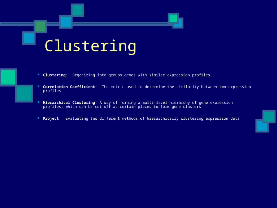
Clustering: Organizing into groups genes with similar expression profiles

Correlation Coefficient: The metric used to determine the similarity between two expression profiles

Hierarchical Clustering: A way of forming a multi-level hierarchy of gene expression profiles, which can be cut off at certain places to form gene clusters

Project: Evaluating two different methods of hierarchically clustering expression data

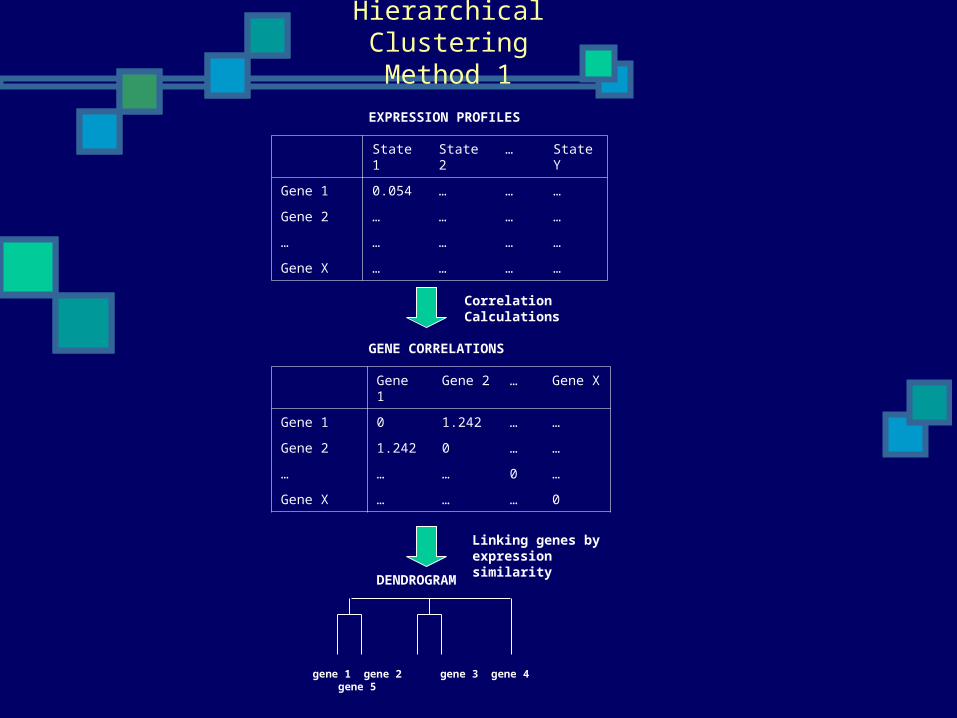
Hierarchical ClusteringMethod 1

State 1 State 2 … State Y

Gene 1 0.054 … … …

Gene 2 … … … …

… … … … …

Gene X … … … …

Correlation Calculations

Gene 1 Gene 2 … Gene X

Gene 1 0 1.242 … …

Gene 2 1.242 0 … …

… … … 0 …

Gene X … … … 0

EXPRESSION PROFILES

GENE CORRELATIONS

gene 1 gene 2 gene 3 gene 4 gene 5

Linking genes by expression similarity

DENDROGRAM

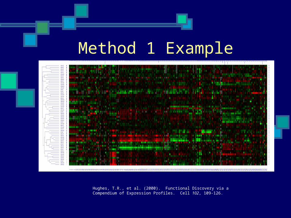
Method 1 Example

Hughes, T.R., et al. (2000). Functional Discovery via a Compendium of Expression Profiles. Cell 102, 109-126.

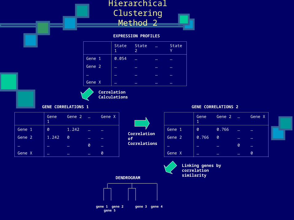
Hierarchical ClusteringMethod 2

State 1 State 2 … State Y

Gene 1 0.054 … … …

Gene 2 … … … …

… … … … …

Gene X … … … …

Correlation Calculations

Gene 1 Gene 2 … Gene X

Gene 1 0 1.242 … …

Gene 2 1.242 0 … …

… … … 0 …

Gene X … … … 0

EXPRESSION PROFILES

GENE CORRELATIONS 1

gene 1 gene 2 gene 3 gene 4 gene 5

Linking genes by correlation similarity

DENDROGRAM

GENE CORRELATIONS 2

Correlation of Correlations

Gene 1 Gene 2 … Gene X

Gene 1 0 0.766 … …

Gene 2 0.766 0 … …

… … … 0 …

Gene X … … … 0

Method 2 Example

Provided by Matteo Pelligrini, Protein Pathways.

Applications of Clustering

Functional Genomics: Gaining information about the possible function of genes with unknown function

Looking at the function of genes that cluster together with genes of unknown function

Diagnostics: Tissues from clinical samples can be clustered together to determine disease subtypes (e.g. tumor classification)

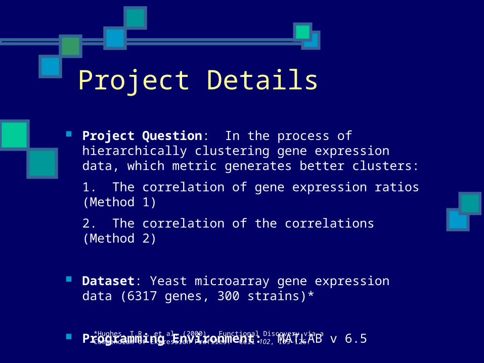
Project Details

Project Question: In the process of hierarchically clustering gene expression data, which metric generates better clusters:

1. The correlation of gene expression ratios (Method 1)

2. The correlation of the correlations (Method 2)

Dataset: Yeast microarray gene expression data (6317 genes, 300 strains)*

Programming Environment: MATLAB v 6.5*Hughes, T.R., et al. (2000). Functional Discovery via a Compendium of Expression Profiles. Cell 102, 109-126.

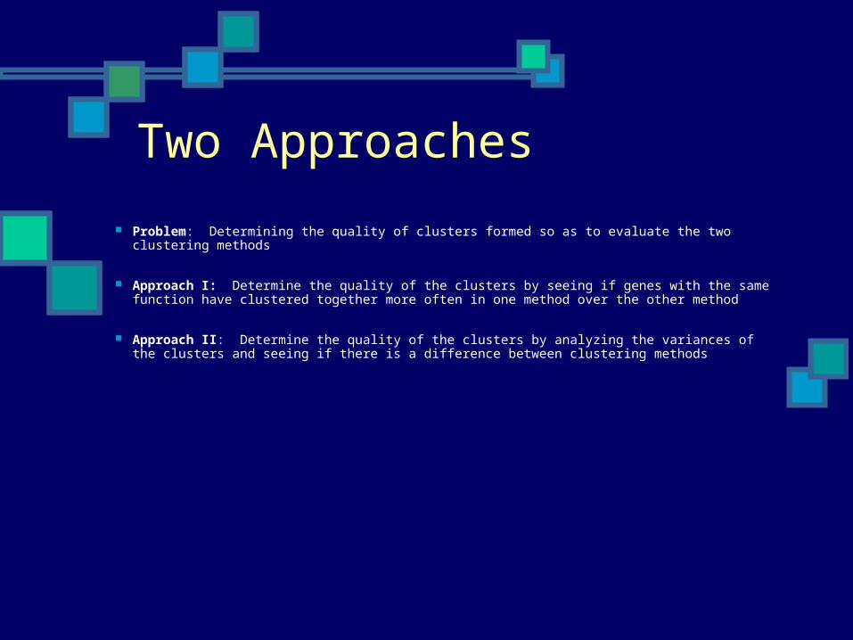
Two Approaches

Problem: Determining the quality of clusters formed so as to evaluate the two clustering methods

Approach I: Determine the quality of the clusters by seeing if genes with the same function have clustered together more often in one method over the other method

Approach II: Determine the quality of the clusters by analyzing the variances of the clusters and seeing if there is a difference between clustering methods

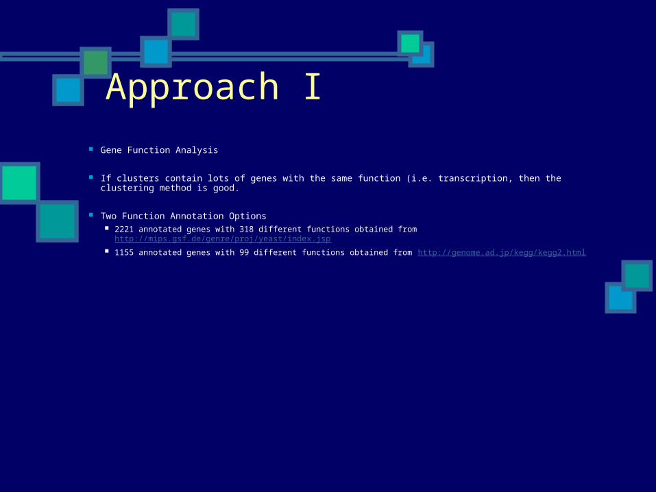
Approach I Gene Function Analysis

If clusters contain lots of genes with the same function (i.e. transcription, then the clustering method is good.

Two Function Annotation Options 2221 annotated genes with 318 different functions obtained from

http://mips.gsf.de/genre/proj/yeast/index.jsp 1155 annotated genes with 99 different functions obtained from http://genome.ad.jp/kegg/kegg2.html

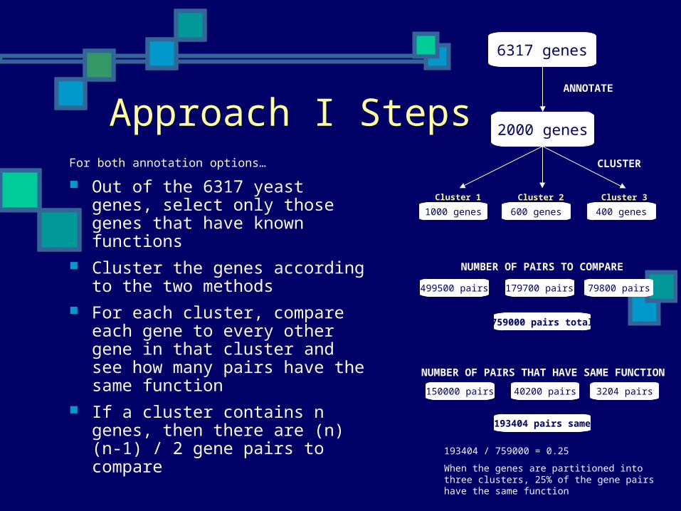
Approach I StepsFor both annotation options…

Out of the 6317 yeast genes, select only those genes that have known functions

Cluster the genes according to the two methods

For each cluster, compare each gene to every other gene in that cluster and see how many pairs have the same function

If a cluster contains n genes, then there are (n)(n-1) / 2 gene pairs to compare

6317 genes

2000 genes

ANNOTATE

1000 genes 600 genes 400 genes

CLUSTER

Cluster 1 Cluster 2 Cluster 3

499500 pairs 179700 pairs 79800 pairs

NUMBER OF PAIRS TO COMPARE

NUMBER OF PAIRS THAT HAVE SAME FUNCTION

759000 pairs total

150000 pairs 40200 pairs 3204 pairs

193404 pairs same

193404 / 759000 = 0.25

When the genes are partitioned into three clusters, 25% of the gene pairs have the same function

Avg % Same vs. No. Clusters

0

0.1

0.2

0.3

0.4

0.5

0.6

0.7

0.8

0.9

1

0 200 400 600 800 1000 1200 1400 1600 1800 2000 2200 2400

Number of Clusters

Ave

rag

e %

Pai

rs w

/ Sam

e F

un

ctio

n

Annotations I, Method I

Annotations I, Method II

Annotations II, Method I

Annotations II, Method II

Approach I Results

Approach II (1):

Determining the quality of the clusters based on their volume.

Comparing the average volume of the clusters generated by method 1 and method 2.

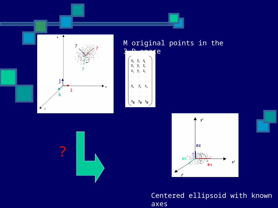
Approach II (2):

If there are M genes in each cluster and for each gene, N experiments are chosen:

We’ll have: M vectors in a N-dimensional space that can be

visualized as M points. The M points generate an ellipsoid if M >

dimensionality of the space. The closer the points to each other, the more

correlated they are together, and the smaller the volume of the cluster.

The smaller the volume of the ellipsoid (cluster), the better the quality of the cluster.

i

j

k

D2

M original points in the 3-D space??

?

?

Centered ellipsoid with known axes

Approach II (3): To compute the volume of the cluster, we first

compute its covariance matrix.

We then use Principal Components Analysis (PCA) to estimate the dimensions of the cluster.

PCA will construct a new space using N orthogonal linear combinations of old vectors of the space. (Each linear combination is a principal component.)

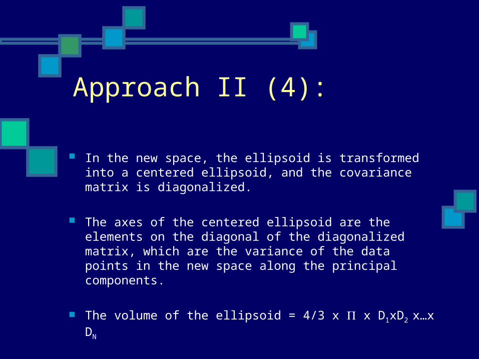
Approach II (4):

In the new space, the ellipsoid is transformed into a centered ellipsoid, and the covariance matrix is diagonalized.

The axes of the centered ellipsoid are the elements on the diagonal of the diagonalized matrix, which are the variance of the data points in the new space along the principal components.

The volume of the ellipsoid = 4/3 x x D1xD2 x…x DN

i

j

k

D1

D2

D3

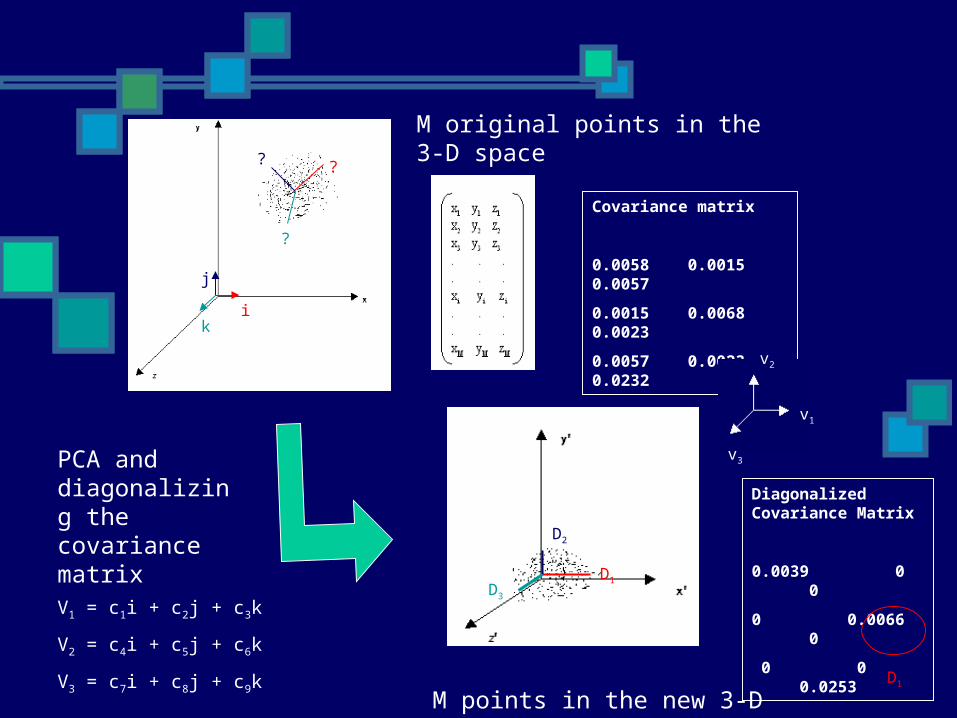
PCA and diagonalizing the covariance matrix

M points in the new 3-D space

M original points in the 3-D space

V1 = c1i + c2j + c3k

V2 = c4i + c5j + c6k

V3 = c7i + c8j + c9k

??

?

Covariance matrix

0.0058 0.0015 0.0057

0.0015 0.0068 0.0023

0.0057 0.0023 0.0232

Diagonalized Covariance Matrix

0.0039 0 0

0 0.0066 0

0 0 0.0253

D1

v1

v2

v3

Approach II (5):

Question: Is one of the methods systematically

generating smaller ellipsoids?

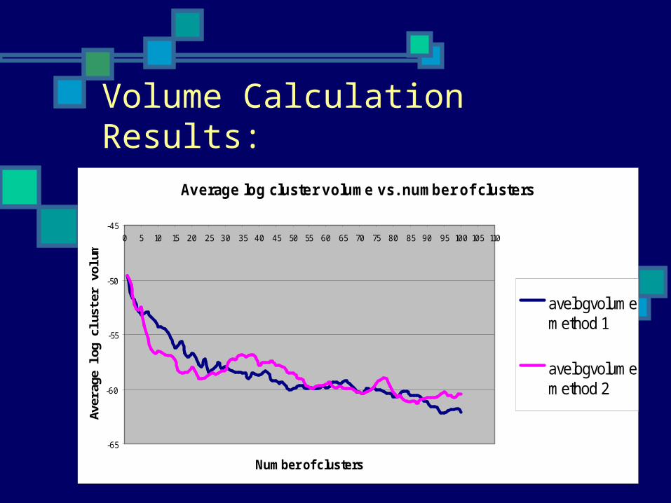
Volume Calculation Results:

Average log cluster volume vs. number of clusters

-65

-60

-55

-50

-450 5 10 15 20 25 30 35 40 45 50 55 60 65 70 75 80 85 90 95 100 105 110

Number of clusters

Ave

rage

log

clus

ter

volu

me

avelogvolumemethod 1

avelogvolumemethod 2

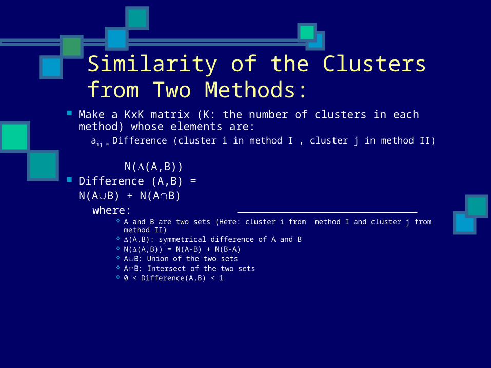
Similarity of the Clusters from Two Methods:

Make a KxK matrix (K: the number of clusters in each method) whose elements are:

aij = Difference (cluster i in method I , cluster j in method II)

N((A,B)) Difference (A,B) =

N(AB) + N(AB) where:

A and B are two sets (Here: cluster i from method I and cluster j from method II) (A,B): symmetrical difference of A and B N((A,B)) = N(A-B) + N(B-A) AB: Union of the two sets AB: Intersect of the two sets 0 < Difference(A,B) < 1

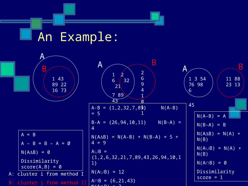
1 2 6 32 21

7 89 43

A B26 94 10 11

A-B = {1,2,32,7,89} N(A-B) = 5

B-A = {26,94,10,11} N(B-A) = 4

N(AB) = N(A-B) + N(B-A) = 5 + 4 = 9

AB = {1,2,6,32,21,7,89,43,26,94,10,11}

N(AB) = 12

AB = {6,21,43} N(AB) = 3

Dissimilarity score (A,B) = 9/(12 + 3 ) = 0.6

1 43 89 22 16 73

B

A

A = B

A – B = B – A = Ø

N(AB) = 0

Dissimilarity score(A,B) = 0

BA1 3 54 76 98 6

45

11 88 23 13

N(A-B) = A

N(B-A) = B

N(AB) = N(A) + N(B)

N(AB) = N(A) + N(B)

N(AB) = 0

Dissimilarity score = 1

An Example:

A: cluster i from method I

B: cluster j from method II

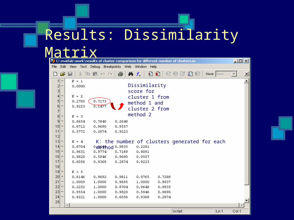
Results: Dissimilarity Matrix

Dissimilarity score for cluster 1 from method 1 and cluster 2 from method 2

K: the number of clusters generated for each method

Discussion and Conclusion (1):

Conclusions: Neither approach can favor one method over the

other with certainty; however, Approach I favors method I when the number of

clusters is small. In the range of 1-100 clusters, while approach I

favors method I, approach II fluctuates in choosing the better method or the other.

The efficiency of both approaches in clustering genes is dependant on the number of clusters.

The similarity of the clusters from method I and method II decreases as the number of clusters increases; in fact, the two methods generate very different clusters.

Discussion and Conclusion (2): Problems faced and future questions:

What is the best cutoff value for clustering? In approach I, not all genes were annotated,

so around 2/3 of the dataset was ignored. Gene annotations are somewhat arbitrary. What are other ways to quantify the quality

of clusters? Memory problem: We couldn’t include all the

genes and all the experiments at the same time to analyze the quality of clusters.

Acknowledgments:

Special thanks to: Our mentor: Dr. Matteo Pellegrini Protein Pathways team:

Dr. Darin Taverna Dr. Peter BowersDr. Mike Thompson Leon Kopelevich

SoCalBSI faculty: Dr. Jamil Momand Dr. Silvia Heubach Dr. Sandra Sharp Dr. Elizabeth Torres

Dr. Wendie Johnston Dr. Jennifer Faust Dr. Nancy Warter-Perez Dr. Beverly Krilowicz

NIH and NSF : whose funding made this internship possible.

Appendix I: Covariance (1)

The covariance of two features is the measure of how the two features vary together. If they both have an increasing or decreasing trend,

c ij> 0.

If one decreases while the other one increases, c ij < 0.

If the changes of one is independent of the changes of the other, c ij = 0.

*

*: http://www.engr.sjsu.edu/~knapp/HCIRODPR/PR_Mahal/cov.htm

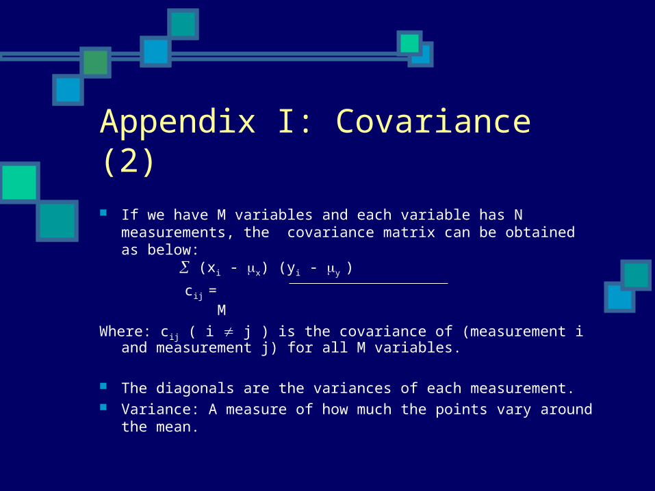
Appendix I: Covariance (2)

If we have M variables and each variable has N measurements, the covariance matrix can be obtained as below: (xi - x) (yi - y )

cij = M

Where: cij ( i j ) is the covariance of (measurement i and measurement j) for all M variables.

The diagonals are the variances of each measurement. Variance: A measure of how much the points vary around the

mean.

Appendix I: Diagonalizing The Covariance Matrix

data =

-0.0300 0.2500 0.0340

0.1430 0.2230 0.1900

-0.0230 0.0410 -0.0110

-0.0060 0.1780 0.3100

-0.0400 0.2120 -0.0560

covariance_data = cov(data);

covariance_data =

0.0058 0.0015 0.0057

0.0015 0.0068 0.0023

0.0057 0.0023 0.0232Covariance matrix

[V, D] = eig (covariance_data); Diagonalize the Covariance matrix

D =

0.0039 0 0

0 0.0066 0

0 0 0.0253

V =

-0.9285 -0.2370 0.2859

0.2856 -0.9478 0.1417

0.2374 0.2133 0.9477

(xi - x) (yi - y )

cij =

M

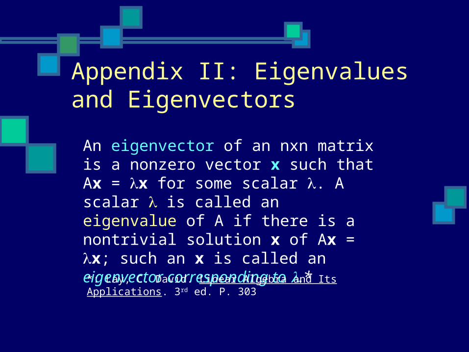
Appendix II: Eigenvalues and Eigenvectors

An eigenvector of an nxn matrix is a nonzero vector x such that Ax = x for some scalar . A scalar is called an eigenvalue of A if there is a nontrivial solution x of Ax = x; such an x is called an eigenvector corresponding to .*

*: Lay, C. David. Linear Algebra and Its Applications. 3rd ed. P. 303

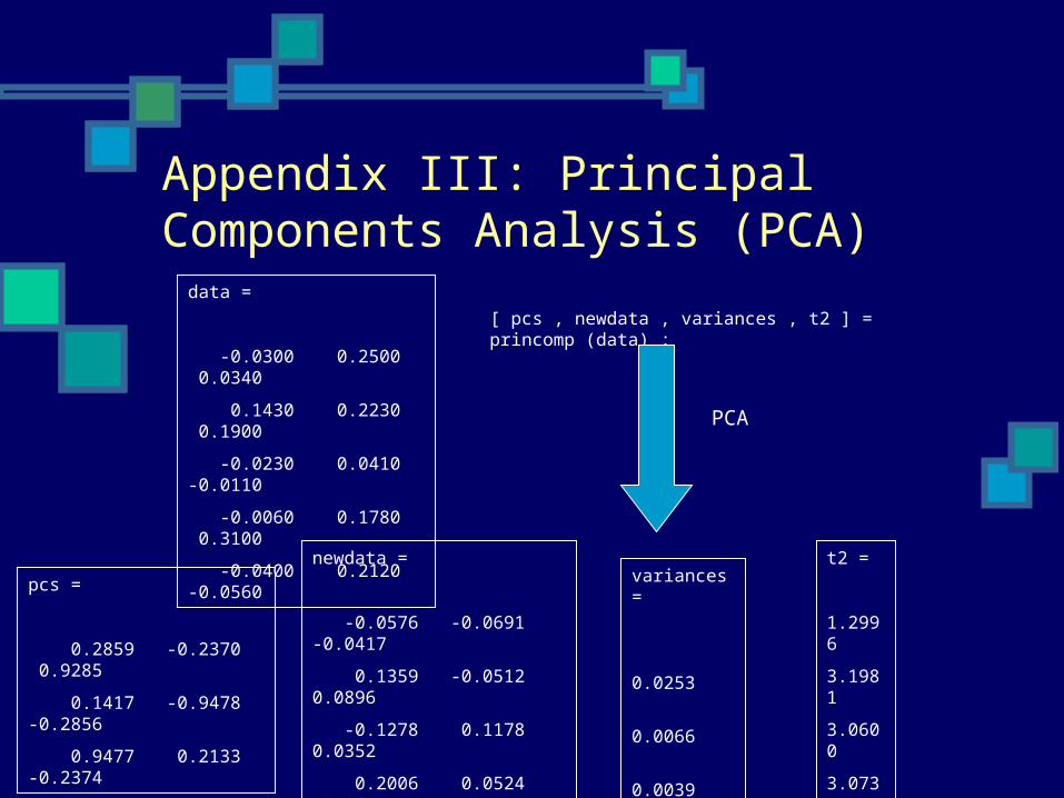
Appendix III: Principal Components Analysis (PCA)

data =

-0.0300 0.2500 0.0340

0.1430 0.2230 0.1900

-0.0230 0.0410 -0.0110

-0.0060 0.1780 0.3100

-0.0400 0.2120 -0.0560

[ pcs , newdata , variances , t2 ] = princomp (data) ;

PCA

pcs =

0.2859 -0.2370 0.9285

0.1417 -0.9478 -0.2856

0.9477 0.2133 -0.2374

newdata =

-0.0576 -0.0691 -0.0417

0.1359 -0.0512 0.0896

-0.1278 0.1178 0.0352

0.2006 0.0524 -0.0644

-0.1511 -0.0499 -0.0188

variances =

0.0253

0.0066

0.0039

t2 =

1.2996

3.1981

3.0600

3.0737

1.3686

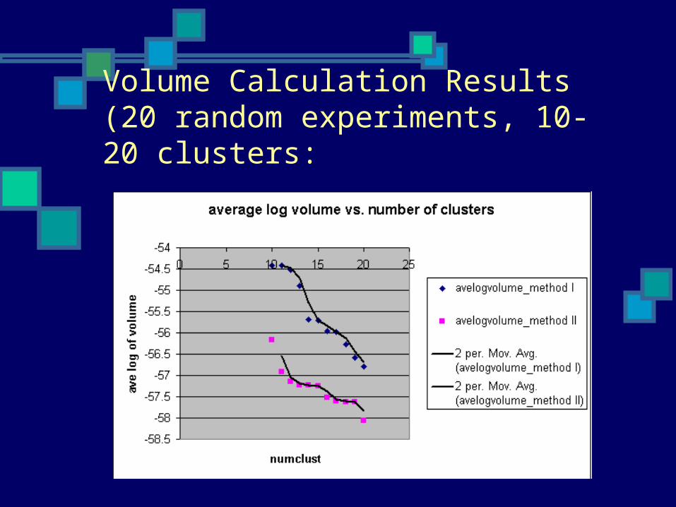
Volume Calculation Results (20 random experiments, 10-20 clusters:

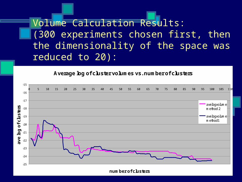
Volume Calculation Results: (300 experiments chosen first, then the dimensionality of the space was reduced to 20):

Average log of cluster volumes vs. number of clusters

-25

-24

-23

-22

-21

-20

-19

-18

-17

-16

-15

0 5 10 15 20 25 30 35 40 45 50 55 60 65 70 75 80 85 90 95 100 105 110

number of clusters

av

e lo

g o

f c

lus

ters

avelogvolumemethod 2

avelogvolumemethod1

Method 1 vs. Method 2 in a More Conceptual View:

Method 1 links together the two genes that have the most similar expression patterns.

Method 2 links together the two genes whose correlation with all other genes is most similar; i.e. it looks at a genes in a more global view (in a context of all other genes).

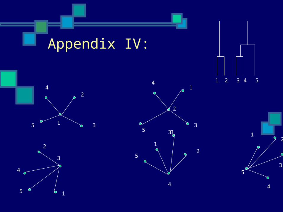
Appendix IV:

1

2

3

4

55

3

14

2

1

2

4

5

3

4

21

3

5

5

12

3

4

3

1 2 3 4 5