Evaluation of the Subsea Compression Project at Gullfaks C

1 | P a g e

Evaluation of the Subsea Compression Project at Gullfaks C

Experts in Teamwork, Gullfaks Village 2013

By group 2

Guidion Mavundla, Joao Silva Unguana, Jonas M. Engebretsen, Thomas Shepherd, Elshan Jabrayilov and Håvard H. Normann

Trondheim, 2 May 2013

2 | P a g e

Summary During one semester, this group of six graduate students have attempted to evaluate the technical

and economic feasibility of the Gullfaks C subsea compressor project. Gullfaks C is a large oil and gas

field on the Norwegian Continental Shelf and is operated by Statoil. Statoil has in cooperation with

Framo Engineering developed a subsea compressor, which goal is to increase the recovery factor and

profitability of the field. Our assignment has been to redo their calculation with simple means.

From our simplified reservoir-model, we have found that the subsea compressor project, given the

assumptions we have made and the input we have been given, is indeed both technically feasible and

economically sensible. The expected profit from the project is estimated to be around NOK 1.7bn,

when compared to the optimal outcome when the templates are running their natural course. The

project is estimated to reach break-even in 2020 and from thereon generate steady profits.

Optimising the timing of pressure reduction in the separator, we found that the separator pressure

should be reduced from 65 to 25 bar in 2020, more specifically in the first quarter.

We have been using a simplified dry-gas and tank-model to estimate the production profile of both

templates and the corresponding pressure development in the respective reservoirs. This simple

model has been extended to encapsulate black-oil properties and give a better estimate of

condensate production. We have made several simplifying assumptions in order give a sound

estimate, enabling us to find results although limited by time, tools and resources.

The largest economic risks, measured in impact on profits, are related to revenue losses due to

increased downtime. These losses outweigh both cost overruns and installation delays. Risks

concerning external input factors such as fluctuations in commodity prices and exchange rates may in

worst case scenarios have substantial effects on profit, but these risks can easily be hedged through

derivatives contracts the financial markets.

The economic risks are the primarily related to technological risks. Increased downtime may be a

result of unforeseen difficulties with installation, maintenance, materials and a number of other

sources of malfunctions. As the subsea compressor is a completely new technology for Statoil and

Framo Engineering to use, the probability of such events to occur is fairly high. However, cost

increases and revenue losses generated from such unforeseen events may be considered an

investment in the technology itself. A successful installation at Gullfaks C, even if met with

difficulties, can be utilized in other fields and increase the recovery rates. Hence, an isolated profit

reduction or loss at Gullfaks C may still result in overall profits for Statoil. We therefore conclude that

the risk/reward ratio of the subsea compressor project is both attractive and sound.

3 | P a g e

Table of Contents Summary ................................................................................................................................................. 2

1 Introduction ..................................................................................................................................... 5

1.1 About the assignment ............................................................................................................. 5

1.2 Background .............................................................................................................................. 5

1.3 Purpose of the problem .......................................................................................................... 5

1.4 Limitations and constraints ..................................................................................................... 5

1.4.1 Reference case ................................................................................................................ 6

1.4.2 Optimised reference case ................................................................................................ 6

1.4.3 Compressor case ............................................................................................................. 6

2 Discussion ........................................................................................................................................ 7

2.1 Methods .................................................................................................................................. 7

2.1.1 Overview of the field and templates ............................................................................... 7

2.1.2 Technical and physical assumptions and simplifications ................................................ 8

2.1.3 The dry-gas model ........................................................................................................... 8

2.1.4 Material balance and black-oil properties .................................................................... 12

2.1.5 HYSYS ............................................................................................................................. 12

2.1.6 Compressor value estimation ........................................................................................ 13

2.1.7 Economic assumptions .................................................................................................. 13

2.2 Procedures and execution ..................................................................................................... 15

2.2.1 Finding the optimal timing of reducing separator pressure ......................................... 15

2.2.2 Computing the compressor production profile ............................................................. 15

2.2.3 Calculation of sensitivities ............................................................................................. 15

2.3 Modelling results ................................................................................................................... 16

2.3.1 Field lifetime and reservoir pressure development ...................................................... 16

2.3.2 Black oil properties vs. dry gas assumptions ................................................................. 20

2.3.3 Optimal timing of LP-modification in the compressor case .......................................... 21

2.3.4 Compressor value in optimal scenario .......................................................................... 22

2.3.5 Sensitivity to changed assumptions .............................................................................. 22

2.3.6 Project risk and risk factors ........................................................................................... 24

3 Conclusions .................................................................................................................................... 26

4 Recommendations......................................................................................................................... 28

5 Appendices .................................................................................................................................... 29

A. Z-factor calculations .................................................................................................................. 29

4 | P a g e

B. Detailed discussion on black-oil properties ............................................................................... 29

B.1 Traditional black oil formulation ....................................................................................... 29

B.2 Modified Black-Oil (MBO) Formulation ............................................................................. 30

B.3 Surface gravities ................................................................................................................ 32

B.4 Reservoir Material Balance – MBO PVT ............................................................................ 32

6 References ..................................................................................................................................... 35

5 | P a g e

1 Introduction

1.1 About the assignment With diminishing petroleum reserves the recovery rate becomes increasingly important. To ensure

that Statoil deliver some of the highest recovery rates in the world they have to pioneer technical

solutions.

This project aims to verify or disprove the validity of an on-going subsea compressor project

conducted by Statoil in cooperation with Framo Engineering (“Framo”). To conduct the project a

multi–national, multi-disciplinary project group was formed as part of the mandatory NTNU graduate

course “Experts in Teamwork” (“EiT”).

The main focus of the project was chosen emphasising the economical perspective of the project. In

order to solve different scenarios and given cases, various models describing how production rates

evolve were made. The economic evaluation was conducted based on these models as well as

various assumptions and supplied information.

1.2 Background Gullfaks is an oil and gas field in the Norwegian sector of the North Sea operated by Statoil. Situated

in block 34/10 with a water depths ranging from 135 - 220 meters, production started in 1986 (Store

Norske Leksikon). The initial recoverable reserves were 2.1 billion barrels, an amount that had

depleted to 234 million barrels by 2004. Peak production was achieved in 2001 with a production

rate of 180,000 barrels per day. The initial expected oil recovery was estimated to be 44% of in-place

volumes. The expected recovery was increased to 61% due to several factors, the main factors being;

well maintenance, reservoir knowledge, technology advances and lower residual oil saturation. The

ambition is to increase it upwards 70%. (Statoil, 2013)

1.3 Purpose of the problem The main objective of the Gullfaks Village is to help Statoil increase the recovery factor of oil and gas

at the Gullfaks field. This year we are to verify Statoil’s evaluation of the project by the use of fairly

simple means. That is, that it is both technically feasible and profitable. This is useful because it may

potentially be a useful screening tool for Statoil to get a quick overview in a portfolio of several

potential projects. Given that our results are in line with Statoil’s own estimates, Statoil may develop

their own routines and models for quick-and-dirty economic analysis.

1.4 Limitations and constraints In order to evaluate the value of the project a reference case had to be made. Also different

scenarios with different parameters were necessary to evaluate the sensitivities of the project.

Therefore the limitations and constraints of each case had to be defined.

6 | P a g e

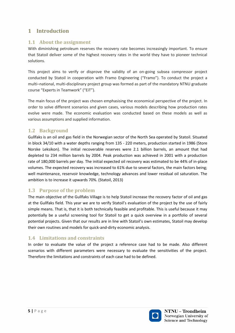
1.4.1 Reference case

Year Template-M Template-L Maximum total daily production

Downtime Pipeline from towhead

Separator pressure

2008-2012 - - 10 MSm3/d 10% 14” 65 2012-2018 Target

production 4 MSm3/d

Target production 6 MSm3/d

10 MSm3/d 10% 14” 65

2018-2029 - - 5 MSm3/d 10% 14” 25 Table 1 Limitations and constraints for the reference case

Also, the minimum daily production said to be economically feasible by Statoil is 2 MSm3/d.

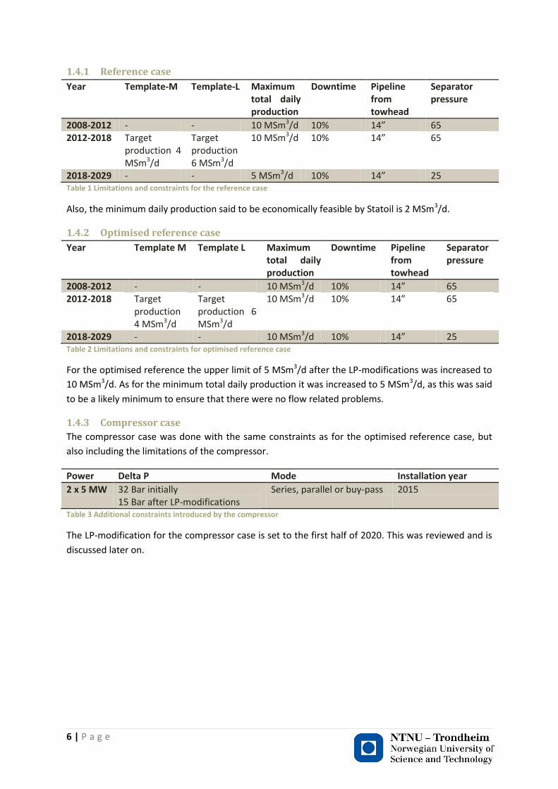
1.4.2 Optimised reference case

Year Template M Template L Maximum total daily production

Downtime Pipeline from towhead

Separator pressure

2008-2012 - - 10 MSm3/d 10% 14” 65 2012-2018 Target

production 4 MSm3/d

Target production 6 MSm3/d

10 MSm3/d 10% 14” 65

2018-2029 - - 10 MSm3/d 10% 14” 25 Table 2 Limitations and constraints for optimised reference case

For the optimised reference the upper limit of 5 MSm3/d after the LP-modifications was increased to

10 MSm3/d. As for the minimum total daily production it was increased to 5 MSm3/d, as this was said

to be a likely minimum to ensure that there were no flow related problems.

1.4.3 Compressor case

The compressor case was done with the same constraints as for the optimised reference case, but

also including the limitations of the compressor.

Power Delta P Mode Installation year

2 x 5 MW 32 Bar initially 15 Bar after LP-modifications

Series, parallel or buy-pass 2015

Table 3 Additional constraints introduced by the compressor

The LP-modification for the compressor case is set to the first half of 2020. This was reviewed and is

discussed later on.

7 | P a g e

2 Discussion

2.1 Methods

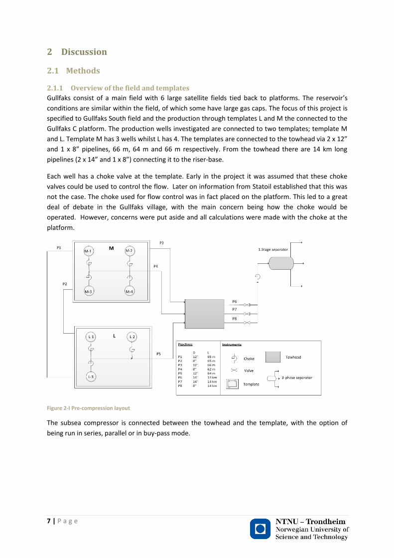
2.1.1 Overview of the field and templates

Gullfaks consist of a main field with 6 large satellite fields tied back to platforms. The reservoir’s

conditions are similar within the field, of which some have large gas caps. The focus of this project is

specified to Gullfaks South field and the production through templates L and M the connected to the

Gullfaks C platform. The production wells investigated are connected to two templates; template M

and L. Template M has 3 wells whilst L has 4. The templates are connected to the towhead via 2 x 12”

and 1 x 8” pipelines, 66 m, 64 m and 66 m respectively. From the towhead there are 14 km long

pipelines (2 x 14” and 1 x 8”) connecting it to the riser-base.

Each well has a choke valve at the template. Early in the project it was assumed that these choke

valves could be used to control the flow. Later on information from Statoil established that this was

not the case. The choke used for flow control was in fact placed on the platform. This led to a great

deal of debate in the Gullfaks village, with the main concern being how the choke would be

operated. However, concerns were put aside and all calculations were made with the choke at the

platform.

Figure 2-I Pre-compression layout

The subsea compressor is connected between the towhead and the template, with the option of

being run in series, parallel or in buy-pass mode.

8 | P a g e

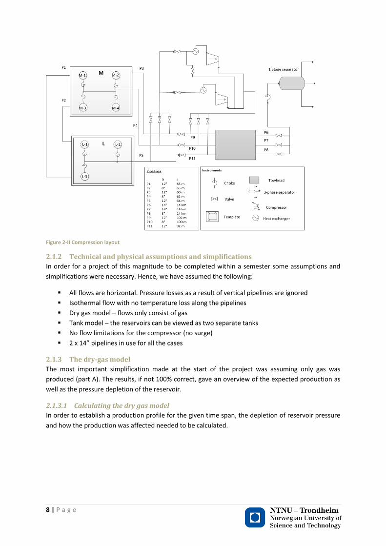
Figure 2-II Compression layout

2.1.2 Technical and physical assumptions and simplifications

In order for a project of this magnitude to be completed within a semester some assumptions and

simplifications were necessary. Hence, we have assumed the following:

All flows are horizontal. Pressure losses as a result of vertical pipelines are ignored

Isothermal flow with no temperature loss along the pipelines

Dry gas model – flows only consist of gas

Tank model – the reservoirs can be viewed as two separate tanks

No flow limitations for the compressor (no surge)

2 x 14” pipelines in use for all the cases

2.1.3 The dry-gas model

The most important simplification made at the start of the project was assuming only gas was

produced (part A). The results, if not 100% correct, gave an overview of the expected production as

well as the pressure depletion of the reservoir.

2.1.3.1 Calculating the dry gas model

In order to establish a production profile for the given time span, the depletion of reservoir pressure

and how the production was affected needed to be calculated.

9 | P a g e

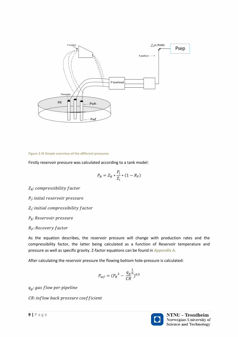
Figure 2-III Simple overview of the different pressures

Firstly reservoir pressure was calculated according to a tank model:

( )

As the equation describes, the reservoir pressure will change with production rates and the

compressibility factor, the latter being calculated as a function of Reservoir temperature and

pressure as well as specific gravity. Z-factor equations can be found in Appendix A.

After calculating the reservoir pressure the flowing bottom hole-pressure is calculated:

(

)

10 | P a g e

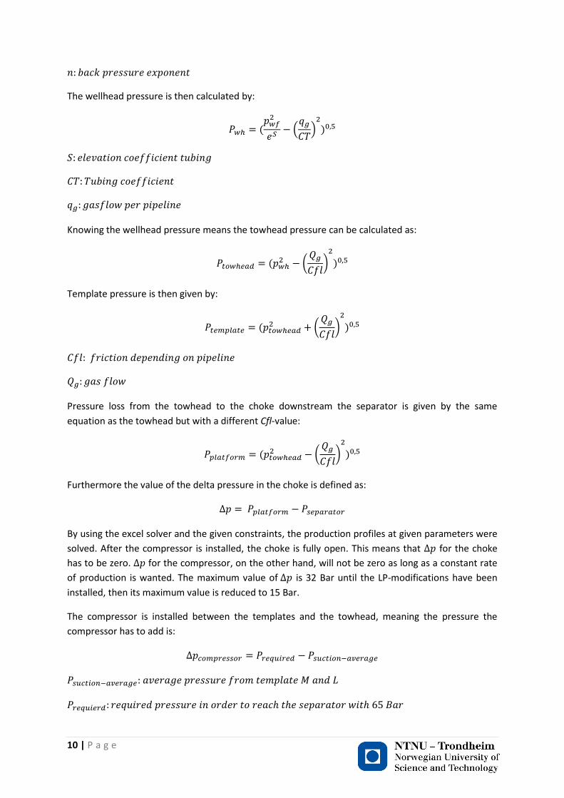
The wellhead pressure is then calculated by:

(

(

)

)

Knowing the wellhead pressure means the towhead pressure can be calculated as:

( (

)

)

Template pressure is then given by:

( (

)

)

Pressure loss from the towhead to the choke downstream the separator is given by the same

equation as the towhead but with a different Cfl-value:

( (

)

)

Furthermore the value of the delta pressure in the choke is defined as:

By using the excel solver and the given constraints, the production profiles at given parameters were

solved. After the compressor is installed, the choke is fully open. This means that for the choke

has to be zero. for the compressor, on the other hand, will not be zero as long as a constant rate

of production is wanted. The maximum value of is 32 Bar until the LP-modifications have been

installed, then its maximum value is reduced to 15 Bar.

The compressor is installed between the templates and the towhead, meaning the pressure the

compressor has to add is:

11 | P a g e

In order to solve the gas flow from each template at the compressor inlet, another constraint was

added to the solver. Making an error function stating that the pressure of each flow could not differ

from the average pressure of the flows ensured that the solver would reach the correct values.

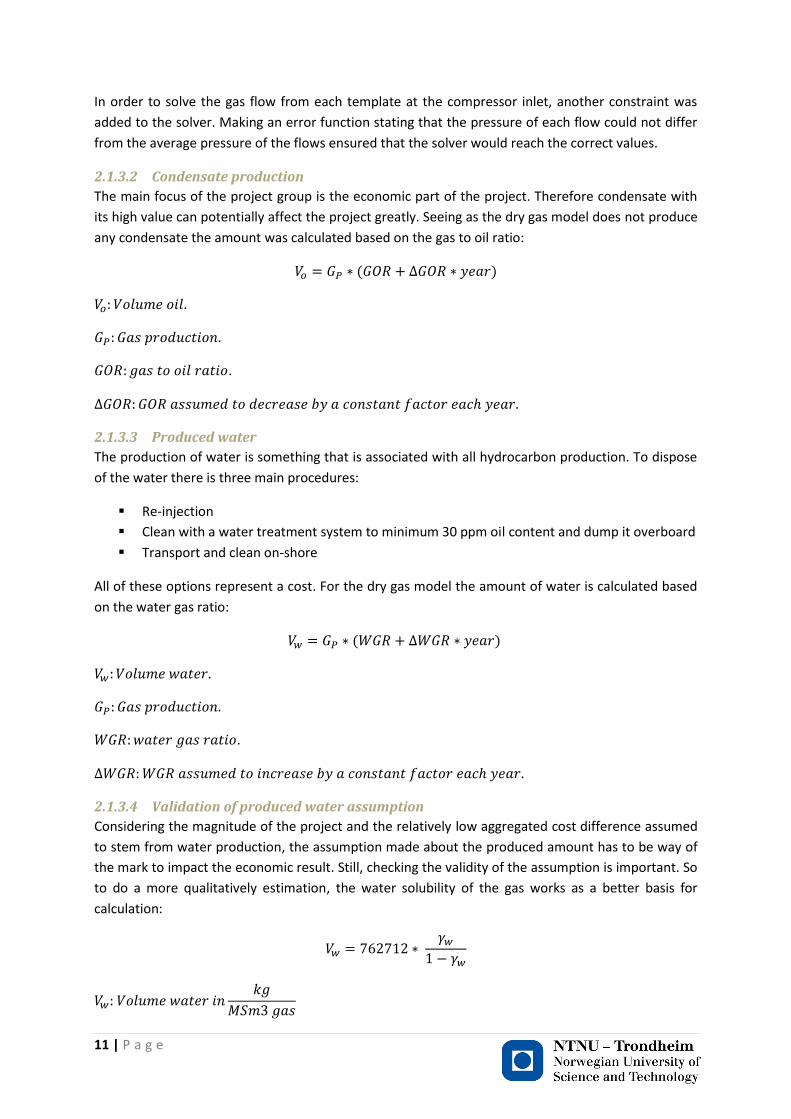
2.1.3.2 Condensate production

The main focus of the project group is the economic part of the project. Therefore condensate with

its high value can potentially affect the project greatly. Seeing as the dry gas model does not produce

any condensate the amount was calculated based on the gas to oil ratio:

( )

.

2.1.3.3 Produced water

The production of water is something that is associated with all hydrocarbon production. To dispose

of the water there is three main procedures:

Re-injection

Clean with a water treatment system to minimum 30 ppm oil content and dump it overboard

Transport and clean on-shore

All of these options represent a cost. For the dry gas model the amount of water is calculated based

on the water gas ratio:

( )

.

2.1.3.4 Validation of produced water assumption

Considering the magnitude of the project and the relatively low aggregated cost difference assumed

to stem from water production, the assumption made about the produced amount has to be way of

the mark to impact the economic result. Still, checking the validity of the assumption is important. So

to do a more qualitatively estimation, the water solubility of the gas works as a better basis for

calculation:

12 | P a g e

( ) ( ) ( )

( )

( )

( ) ( )

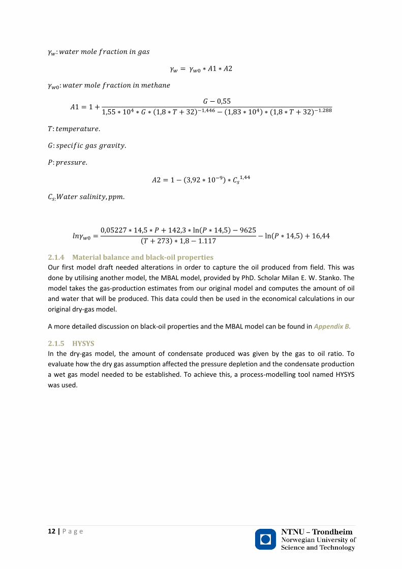
2.1.4 Material balance and black-oil properties

Our first model draft needed alterations in order to capture the oil produced from field. This was

done by utilising another model, the MBAL model, provided by PhD. Scholar Milan E. W. Stanko. The

model takes the gas-production estimates from our original model and computes the amount of oil

and water that will be produced. This data could then be used in the economical calculations in our

original dry-gas model.

A more detailed discussion on black-oil properties and the MBAL model can be found in Appendix B.

2.1.5 HYSYS

In the dry-gas model, the amount of condensate produced was given by the gas to oil ratio. To

evaluate how the dry gas assumption affected the pressure depletion and the condensate production

a wet gas model needed to be established. To achieve this, a process-modelling tool named HYSYS

was used.

13 | P a g e

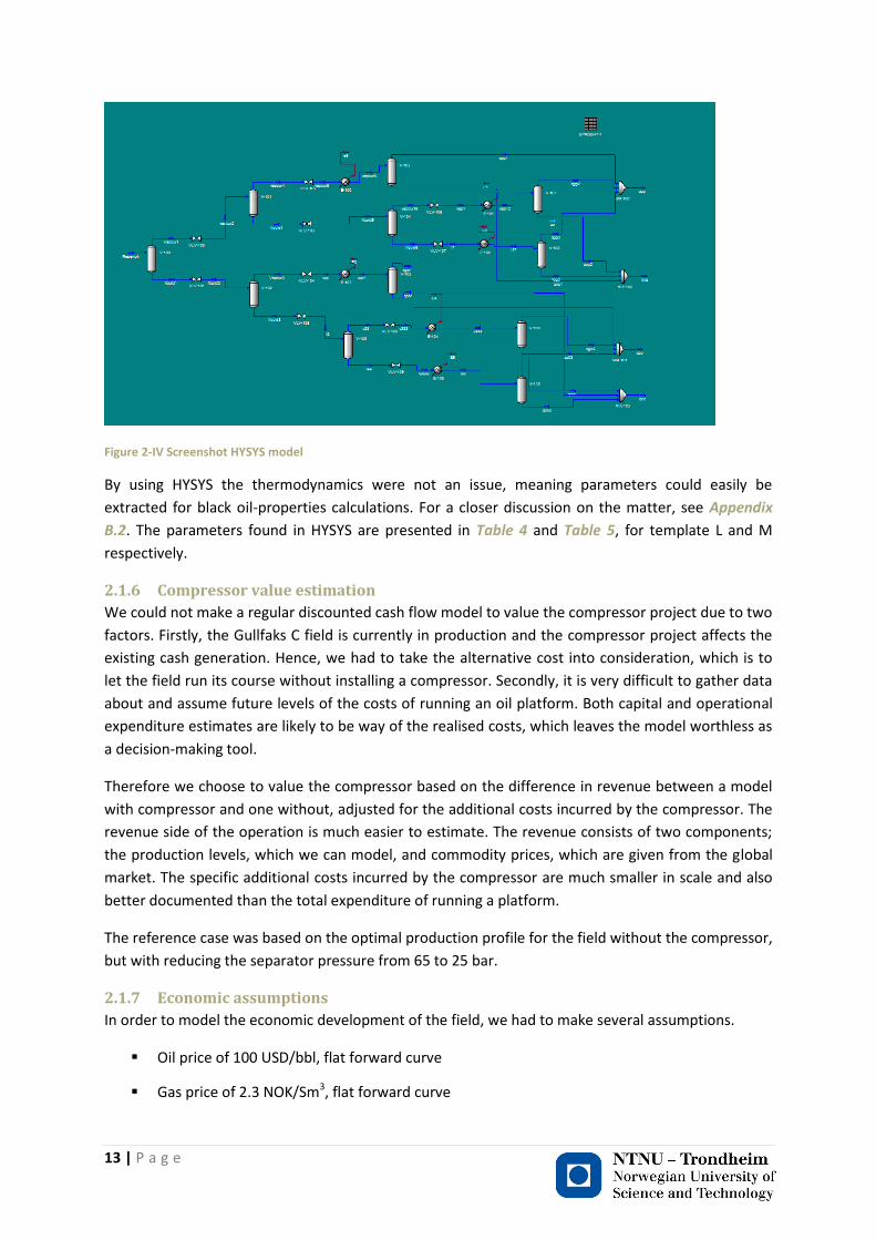
Figure 2-IV Screenshot HYSYS model

By using HYSYS the thermodynamics were not an issue, meaning parameters could easily be

extracted for black oil-properties calculations. For a closer discussion on the matter, see Appendix

B.2. The parameters found in HYSYS are presented in Table 4 and Table 5, for template L and M

respectively.

2.1.6 Compressor value estimation

We could not make a regular discounted cash flow model to value the compressor project due to two

factors. Firstly, the Gullfaks C field is currently in production and the compressor project affects the

existing cash generation. Hence, we had to take the alternative cost into consideration, which is to

let the field run its course without installing a compressor. Secondly, it is very difficult to gather data

about and assume future levels of the costs of running an oil platform. Both capital and operational

expenditure estimates are likely to be way of the realised costs, which leaves the model worthless as

a decision-making tool.

Therefore we choose to value the compressor based on the difference in revenue between a model

with compressor and one without, adjusted for the additional costs incurred by the compressor. The

revenue side of the operation is much easier to estimate. The revenue consists of two components;

the production levels, which we can model, and commodity prices, which are given from the global

market. The specific additional costs incurred by the compressor are much smaller in scale and also

better documented than the total expenditure of running a platform.

The reference case was based on the optimal production profile for the field without the compressor,

but with reducing the separator pressure from 65 to 25 bar.

2.1.7 Economic assumptions

In order to model the economic development of the field, we had to make several assumptions.

Oil price of 100 USD/bbl, flat forward curve

Gas price of 2.3 NOK/Sm3, flat forward curve

14 | P a g e

NOK/USD exchange rate of 6.00 NOK/USD

CAPEX of NOK 1,935mm with a 25-50-25 distribution from signing to installation

Water production cost of 0.60 USD/Sm3

Project specific OPEX of NOK 10mm per year

Cost of reducing separator pressure of NOK 25mm

Cash flows are discounted midyear, to better capture the fact that equal daily levels of cash is generated throughout the year

The first three assumptions are best guesses at the future price of commodities and currencies. We could have used forward curves provided by futures prices from commodity exchanges, but these contracts will generally not cover the lifespan we are looking for. Furthermore, it is not the scope of this assignment to speculate in price developments. Hence, such a simplifying assumption is rational. Although the current NOK/USD exchange rate is lower than what we assume in our model, the historical average over the last 15 years is 6.87 NOK/USD (Norges Bank, 2013). As we are using a flat exchange rate over a period of around 20 years, we found it reasonable to choose a rate closer to the historical average.

The CAPEX estimate is based on the announced contracts for the suppliers Apply Sørco, Nexans, Framo Engineering and Subsea 7. The pay-out-distribution is assumed to be 25% of contract value when the contract is awarded, 50% at completion and 25% after installation. All contracts were awarded in 2012 and installations are expected to be finished by October 2015.

The flat operational expenditure is assigned based on a best guess of increased controller costs and maintenance. Likewise, we assigned a fixed investment of reducing the separator pressure assuming that there will be stops in production and some modification of equipment. Water production costs assumes solid disposal of leftover sludge (Igunnu & Chen, 2012).

The daily production, and hence the cash flows, are nearly identically distributed throughout the year. In order to capture this effect, we use midyear discounting instead of yearend discounting, i.e. we discount the yearly cash flow from July 1 rather than from December 31. This form of discounting is better suited to estimate the true time-value of the cash flows.

15 | P a g e

2.2 Procedures and execution

2.2.1 Finding the optimal timing of reducing separator pressure

The purpose of reviewing the timing of the LP-modifications was to identify what installation date

resulted in the highest NPV. To achieve this, a trial and error approach was chosen. This is a time-

consuming approach, consisting of solving production profiles for LP-modifications at different times.

In order to specify the timing with greater accuracy, the time period in question (2018 – 2021) was

expanded to a higher resolution. This meant to use quarterly instead of yearly time intervals. As for

the constraints, they were the same as for the optimised reference and compressor case. The main

constraints being production shutdown at 5 MSm3/d and a target production rate at 10 MSm3/d.

2.2.2 Computing the compressor production profile

As we are choking from the platform, we cannot choke the wells when the compressor is installed.

Therefore, the flow rates from each template must be adjusted so that pressure on the towhead is

equal for the pipes from both templates. Hence, we must solve for the towhead-pressure for both

templates to be equal, with an allowed error or less than 0.001 bar. Moreover, Δp must be kept less

than its limit of 32 or 15 bar.

2.2.3 Calculation of sensitivities

All these assumptions yield uncertainty. As a way of quantifying the impact of such uncertainty, we

do sensitivity analysis. Different scenarios can be simulated and their impact on the project paired

with the probability of the scenario occurring must be used to assess the born risk. The purpose of a

sensitivity analysis is hence to compute the impact if a given scenario is to occur and make it easy to

compare the various scenarios.

The numerical outcome of changes in assumptions will depend on the resolution of our model. When

calculating the sensitivity of changes, we chose to use yearly intervals. This procedure was chosen for

two reasons. Firstly, it is computationally less expensive and of ease for us, which let us do a larger

variety of sensitivities. Secondly, sensitivities are by nature inaccurate and are used to get a quick

overview of what changes in assumptions will imply.

To explore the compressor project’s sensitivity to increased or decreased capital expenditure, we

multiplied the CAPEX-column of our model by a factor corresponding to the change, i.e. 1.3 and 0.7

respectively. This was done only in compressor case, as there are no project specific costs in the

reference case.

When we calculated the effect of changed installation timing for the compressor, we had to calculate

the new production profile of the well. The gas production was then used as input in the MBAL-

model to get the oil production profile. Furthermore, the installation time also affects the

distribution of CAPEX as well as when we have compressor OPEX. All these data had to be altered as

well.

Increased downtime effect both the daily production levels and the annualised income generated.

Hence, we had to use MBAL to find the corresponding oil production and then alter the production

days-parameter in our model for all subsequent years after the introduction of the compressor.

In order to remove the effect of LP modification, all we had to was to change the required separator

pressure and resolve to find the optimal production profile for the affected years.

16 | P a g e

In addition to the required sensitivity analysis, we chose to explore how the compressor value would

vary with commodity prices; exogenous variables which Statoil cannot affect. This is interesting

because Statoil have many means and influence over installation timing and expenditure. However

when it comes to prices for its products, Statoil must obey the global commodity market. It is

therefore the parameter which Statoil has the least control over.

2.3 Modelling results

2.3.1 Field lifetime and reservoir pressure development

2.3.1.1 Reference case

0

50

100

150

200

250

300

2008 2014 2019 2020 2023 2029

bara Temp L

Reservoir Pwf

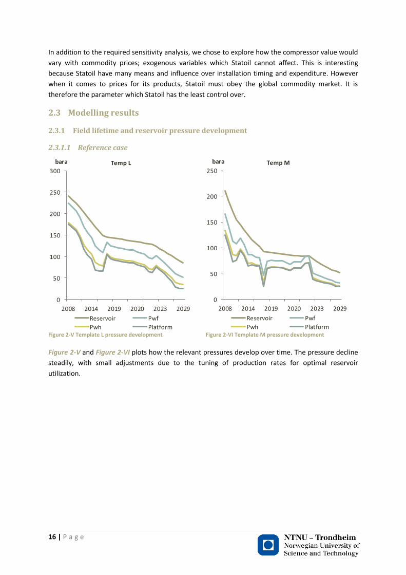
Pwh Platform Figure 2-V Template L pressure development

0

50

100

150

200

250

2008 2014 2019 2020 2023 2029

bara Temp M

Reservoir Pwf

Pwh Platform Figure 2-VI Template M pressure development

Figure 2-V and Figure 2-VI plots how the relevant pressures develop over time. The pressure decline

steadily, with small adjustments due to the tuning of production rates for optimal reservoir

utilization.

17 | P a g e

0

2

4

6

8

10

12

2008 2014 2019 2020 2023 2029

mm Sm3/d

Total production Template L Template M

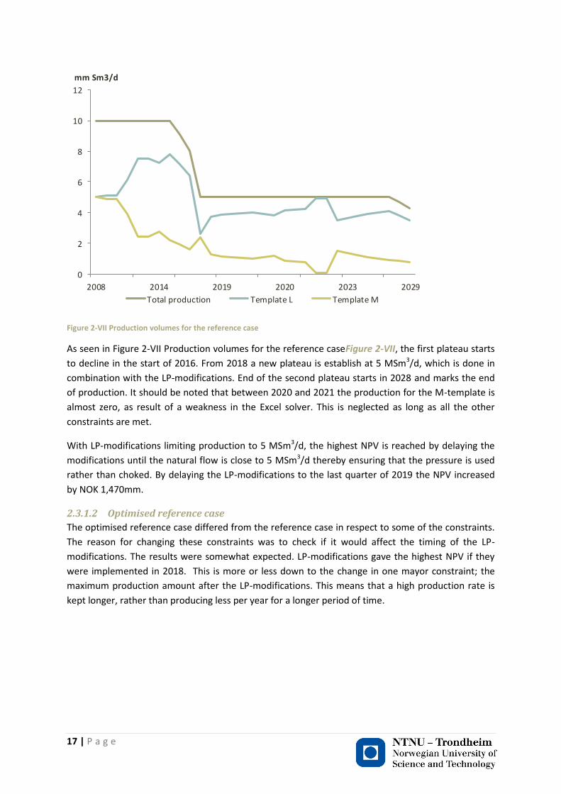
Figure 2-VII Production volumes for the reference case

As seen in Figure 2-VII Production volumes for the reference caseFigure 2-VII, the first plateau starts

to decline in the start of 2016. From 2018 a new plateau is establish at 5 MSm3/d, which is done in

combination with the LP-modifications. End of the second plateau starts in 2028 and marks the end

of production. It should be noted that between 2020 and 2021 the production for the M-template is

almost zero, as result of a weakness in the Excel solver. This is neglected as long as all the other

constraints are met.

With LP-modifications limiting production to 5 MSm3/d, the highest NPV is reached by delaying the

modifications until the natural flow is close to 5 MSm3/d thereby ensuring that the pressure is used

rather than choked. By delaying the LP-modifications to the last quarter of 2019 the NPV increased

by NOK 1,470mm.

2.3.1.2 Optimised reference case

The optimised reference case differed from the reference case in respect to some of the constraints.

The reason for changing these constraints was to check if it would affect the timing of the LP-

modifications. The results were somewhat expected. LP-modifications gave the highest NPV if they

were implemented in 2018. This is more or less down to the change in one mayor constraint; the

maximum production amount after the LP-modifications. This means that a high production rate is

kept longer, rather than producing less per year for a longer period of time.

18 | P a g e

0

50

100

150

200

250

300

2008 2011 2014 2017 2020 2023 2026 2029

bara Temp L

Reservoir Pwf

Pwh Platform Figure 2-VIII Template L pressure development

0

50

100

150

200

250

2008 2011 2014 2017 2020 2023 2026 2029

bara Temp M

Reservoir Pwf

Pwh Platform Figure 2-IX Template M pressure development

0

2

4

6

8

10

12

2008 2011 2014 2017 2020 2023 2026 2029

mm Sm3/d

Total production Template L Template M

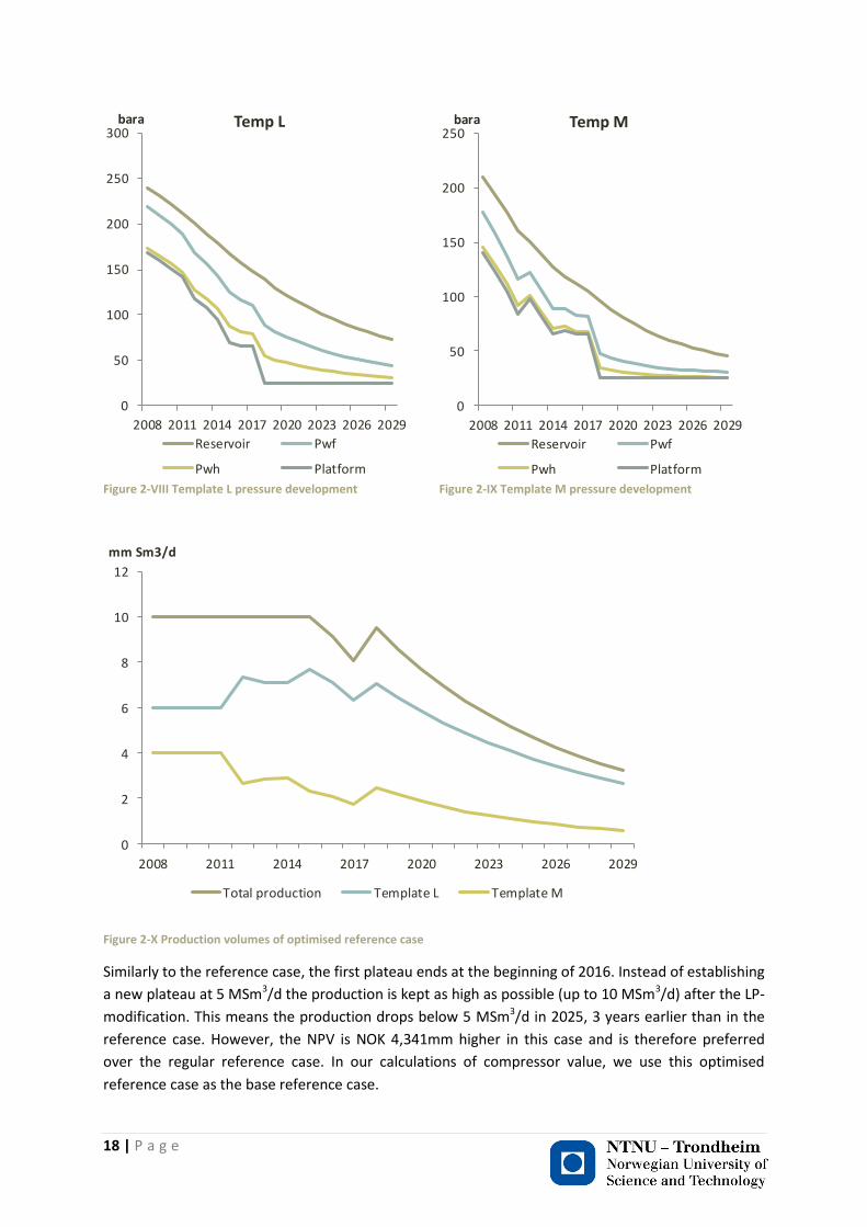
Figure 2-X Production volumes of optimised reference case

Similarly to the reference case, the first plateau ends at the beginning of 2016. Instead of establishing

a new plateau at 5 MSm3/d the production is kept as high as possible (up to 10 MSm3/d) after the LP-

modification. This means the production drops below 5 MSm3/d in 2025, 3 years earlier than in the

reference case. However, the NPV is NOK 4,341mm higher in this case and is therefore preferred

over the regular reference case. In our calculations of compressor value, we use this optimised

reference case as the base reference case.

19 | P a g e

2.3.1.3 Compressor case

0

20

40

60

80

100

120

2008 2011 2014 2017 2020 2023 2026 2029

bara

Temp L choke Temp M choke Suction pressure Compressor delta

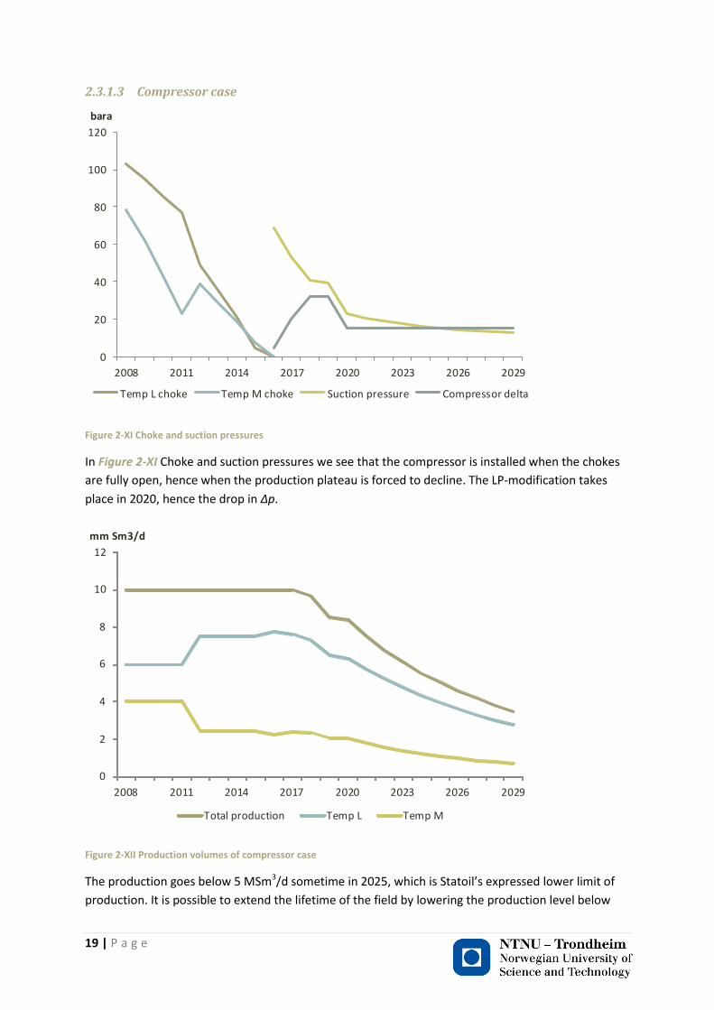
Figure 2-XI Choke and suction pressures

In Figure 2-XI Choke and suction pressures we see that the compressor is installed when the chokes

are fully open, hence when the production plateau is forced to decline. The LP-modification takes

place in 2020, hence the drop in Δp.

0

2

4

6

8

10

12

2008 2011 2014 2017 2020 2023 2026 2029

mm Sm3/d

Total production Temp L Temp M

Figure 2-XII Production volumes of compressor case

The production goes below 5 MSm3/d sometime in 2025, which is Statoil’s expressed lower limit of

production. It is possible to extend the lifetime of the field by lowering the production level below

20 | P a g e

what is optimal in any given year before 2025. This will not change the recovery factor; hence it is

merely delaying the production of the oil and gas in place. This will reduce the aggregated cash flow

of the field, as later income is more heavily discounted.

2.3.2 Black oil properties vs. dry gas assumptions

After adding black oil parameters to the MBAL model with HYSYS input and solving these values in

the given material balance equations, we got the following production profiles:

0

500

1000

1500

2000

2500

3000

3500

0E+0

1E+6

2E+6

3E+6

4E+6

5E+6

6E+6

7E+6

8E+6

9E+6

0 5 10 15

Co

nd

en

sate

pro

du

ctio

n,

[STB

/d]

Gas

pro

du

ctio

n

Years

Gasproduction

Condensateproduct ion

Figure 2-XIII Dry gas and condensate gas production over time for template L

0

200

400

600

800

1000

1200

1400

1600

1800

2000

0E+0

1E+6

2E+6

3E+6

4E+6

5E+6

6E+6

0 5 10 15

Co

nd

en

sate

pro

du

ctio

n,

[STB

/d]

Gas

pro

du

ctio

n

Years

Gasproduction

Condensateproduction

Figure 2-XIV Dry gas and wet (condensate) gas production over time for template M

These production profiles yield the following oil to gas ratios:

0,E+0

1,E-5

2,E-5

3,E-5

4,E-5

5,E-5

6,E-5

7,E-5

8,E-5

9,E-5

1,E-4

60 110 160 210

rs [S

m^3

/Sm

^3]

Reservoir pressure, pr, [bara]

Figure 2-XV Oil/gas ratio against reservoir pressure in template L

0,E+0

1,E-5

2,E-5

3,E-5

4,E-5

5,E-5

6,E-5

7,E-5

8,E-5

9,E-5

1,E-4

60 110 160 210

rs [S

m^3

/Sm

^3]

Reservoir pressure, pr, [bara]

Figure 2-XVI Oil/gas ratio against reservoir pressure in template L

21 | P a g e

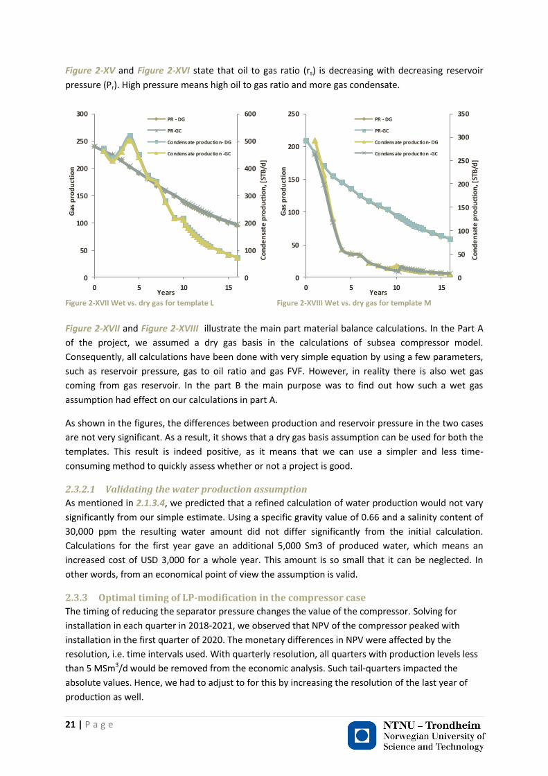
Figure 2-XV and Figure 2-XVI state that oil to gas ratio (rs) is decreasing with decreasing reservoir

pressure (Pr). High pressure means high oil to gas ratio and more gas condensate.

0

100

200

300

400

500

600

0

50

100

150

200

250

300

0 5 10 15

Co

nd

en

sate

pro

du

ctio

n, [

STB

/d]

Gas

pro

du

ctio

n

Years

PR - DG

PR-GC

Condensate production- DG

Condensate production -GC

Figure 2-XVII Wet vs. dry gas for template L

0

50

100

150

200

250

300

350

0

50

100

150

200

250

0 5 10 15

Co

nd

en

sate

pro

du

ctio

n, [

STB

/d]

Gas

pro

du

ctio

n

Years

PR - DG

PR-GC

Condensate production- DG

Condensate production -GC

Figure 2-XVIII Wet vs. dry gas for template M

Figure 2-XVII and Figure 2-XVIII illustrate the main part material balance calculations. In the Part A

of the project, we assumed a dry gas basis in the calculations of subsea compressor model.

Consequently, all calculations have been done with very simple equation by using a few parameters,

such as reservoir pressure, gas to oil ratio and gas FVF. However, in reality there is also wet gas

coming from gas reservoir. In the part B the main purpose was to find out how such a wet gas

assumption had effect on our calculations in part A.

As shown in the figures, the differences between production and reservoir pressure in the two cases

are not very significant. As a result, it shows that a dry gas basis assumption can be used for both the

templates. This result is indeed positive, as it means that we can use a simpler and less time-

consuming method to quickly assess whether or not a project is good.

2.3.2.1 Validating the water production assumption

As mentioned in 2.1.3.4, we predicted that a refined calculation of water production would not vary

significantly from our simple estimate. Using a specific gravity value of 0.66 and a salinity content of

30,000 ppm the resulting water amount did not differ significantly from the initial calculation.

Calculations for the first year gave an additional 5,000 Sm3 of produced water, which means an

increased cost of USD 3,000 for a whole year. This amount is so small that it can be neglected. In

other words, from an economical point of view the assumption is valid.

2.3.3 Optimal timing of LP-modification in the compressor case

The timing of reducing the separator pressure changes the value of the compressor. Solving for

installation in each quarter in 2018-2021, we observed that NPV of the compressor peaked with

installation in the first quarter of 2020. The monetary differences in NPV were affected by the

resolution, i.e. time intervals used. With quarterly resolution, all quarters with production levels less

than 5 MSm3/d would be removed from the economic analysis. Such tail-quarters impacted the

absolute values. Hence, we had to adjust to for this by increasing the resolution of the last year of

production as well.

22 | P a g e

The reason for 2020 being the optimal year to install is that compressor can maintain a Δp of 32 bar

when the separator runs at 65 bar, but is reduced to 15 bar when the separator pressure is reduced.

Hence, by delaying the LP-modification, we can utilise the compressor at full capacity for a longer

period of time. 2020 is shown as the optimal time for modification also with yearly time steps.

2.3.4 Compressor value in optimal scenario

We used our model to compare to financial outcomes of the compressor case and reference case.

Using the methodology described in 2.1.5, we calculated a net present value of NOK 1,723.4mm for

the compressor project in the standard case.

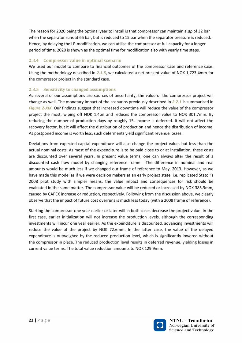
2.3.5 Sensitivity to changed assumptions

As several of our assumptions are sources of uncertainty, the value of the compressor project will

change as well. The monetary impact of the scenarios previously described in 2.2.1 is summarised in

Figure 2-XIX. Our findings suggest that increased downtime will reduce the value of the compressor

project the most, wiping off NOK 1.4bn and reduces the compressor value to NOK 301.7mm. By

reducing the number of production days by roughly 15, income is deferred. It will not affect the

recovery factor, but it will affect the distribution of production and hence the distribution of income.

As postponed income is worth less, such deferments yield significant revenue losses.

Deviations from expected capital expenditure will also change the project value, but less than the

actual nominal costs. As most of the expenditure is to be paid close to or at installation, these costs

are discounted over several years. In present value terms, one can always alter the result of a

discounted cash flow model by changing reference frame. The difference in nominal and real

amounts would be much less if we changed our frame of reference to May, 2013. However, as we

have made this model as if we were decision makers at an early project state, i.e. replicated Statoil’s

2008 pilot study with simpler means, the value impact and consequences for risk should be

evaluated in the same matter. The compressor value will be reduced or increased by NOK 385.9mm,

caused by CAPEX increase or reduction, respectively. Following from the discussion above, we clearly

observe that the impact of future cost overruns is much less today (with a 2008 frame of reference).

Starting the compressor one year earlier or later will in both cases decrease the project value. In the

first case, earlier initialization will not increase the production levels, although the corresponding

investments will incur one year earlier. As the expenditure is discounted, advancing investments will

reduce the value of the project by NOK 72.6mm. In the latter case, the value of the delayed

expenditure is outweighed by the reduced production level, which is significantly lowered without

the compressor in place. The reduced production level results in deferred revenue, yielding losses in

current value terms. The total value reduction amounts to NOK 129.9mm.

23 | P a g e

1,723

-0,386

0,386

-0,073 -0,130

-1,422

0,0

0,5

1,0

1,5

2,0

2,5

Initial + 30% CAPEX - 30% CAPEX -1 Year +1 Year 15%downtime

NOKbn

Figure 2-XIX Value implications in various scenarios

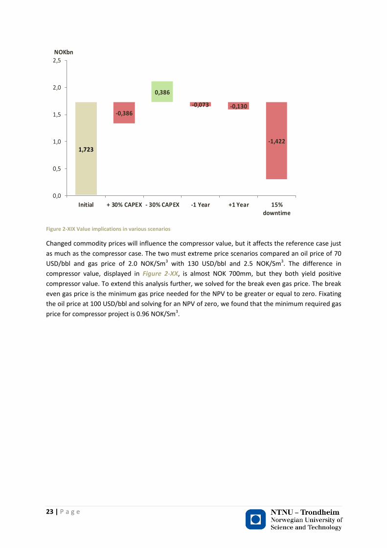
Changed commodity prices will influence the compressor value, but it affects the reference case just

as much as the compressor case. The two must extreme price scenarios compared an oil price of 70

USD/bbl and gas price of 2.0 NOK/Sm3 with 130 USD/bbl and 2.5 NOK/Sm3. The difference in

compressor value, displayed in Figure 2-XX, is almost NOK 700mm, but they both yield positive

compressor value. To extend this analysis further, we solved for the break even gas price. The break

even gas price is the minimum gas price needed for the NPV to be greater or equal to zero. Fixating

the oil price at 100 USD/bbl and solving for an NPV of zero, we found that the minimum required gas

price for compressor project is 0.96 NOK/Sm3.

24 | P a g e

-1,5

-1

-0,5

0

0,5

1

1,5

2

2,5

2008 2011 2014 2017 2020 2023 2026 2029

NOKbn

Price sensitivity

Base case

Figure 2-XX Cumulative net difference in cash flow for compressor- and reference case

2.3.6 Project risk and risk factors

In lack of proper risk calculation tools, adequate experience in the field and the scope of this project,

we are not able to make an extensive and quantitative risk assessment. The following risk analysis is

therefore bases on qualitative measures related to findings in the model and literature on the

matter.

There are several technological risks involved with the subsea compressor project. Although the

compressor has been thoroughly tested and simulated, there is a probability that it will not work

when installed due to errors in the initial design. It is hard to quantify such a risk, but as this is a new

technology it is reasonable to assume that it is significant. On the upside, the efficiency of the

compressor may be higher than expected, boosting the recovery rate.

DNV has listed four key technical areas of risk in subsea compression; the electrical power

distribution systems, the magnetic bearing systems, the high speed rotating machinery and the

control systems. Individual components in the electrical power systems will affect other components,

while high speed rotating machinery puts components under stress and are vulnerable to unwanted

parts in the moving area. These systems are already challenging onshore and the impact of

malfunction and failures are multiplied subsea. (Det Norske Veritas, 2008)

The technical risks translate to economic risks. Unexpected malfunctions are costly and will stall

production, yielding both revenue losses and repair costs. Unplanned production stops are by far the

most costly – 15 more days of maintenance per year from installation wipes of NOK 1.4bn of profits,

without even taking into consideration the potential costs of using vessels, ROVs and additional

personnel. Moreover, cost overruns in both the design and implementation phase will directly affect

the bottom line.

25 | P a g e

The installation will take place subsea with aid from ROVs and not divers. Moreover, no new wells

are drilled and the field is mature. We therefore see little risk when it comes to health, safety and

environment. One can never fully remove any risk in these situations, but Statoil and suppliers on the

Norwegian Continental Shelf already have well-established routines and are under supervision from

a strict regulatory regime, designed to mitigate these risks.

There is also a vast upside in investing in this technology. Although the compressor at Gullfaks should

experience either cost overruns or unexpected downtime, these errors will provide valuable learning

opportunities and experience with the use of subsea compression. Because such knowledge may

reduce the risk when potentially employing the technology on other fields, the risk of isolated losses

on Gullfaks can be outweighed by the reduced risk on future projects. Hence, this technological

investment may be worth more than what our simple NPV-analysis shows in terms of monetary

gains.

The key take-away from the technical side of this risk analysis is that when the compressor first is

installed, errors are extremely costly. As we observed in the sensitivity analysis in 2.3.5 increased

capital expenditure will have much less impact on the value generated from the compressor than

increased downtime. It would therefore be worthwhile to increase spending in order to get it right

from the beginning rather than saving money up front for then to fix problems after installation.

Commodity prices and exchange rates are exogenous variables given by the global capital and

commodity markets. Commodity prices will affect the project value, but even in our worst case

scenario the value is still positive by a large margin. With a break-even gas price of less than 1

NOK/Sm3, this financial risk should not have any implications of decision making and is therefore not

an important risk for the project leaders to pay attention to. This project runs the same financial risks

as Statoil as a whole, as the company’s profitability is highly correlated with commodity prices. This is

the risk exposure investors are paying to get and is Statoil’s value proposition to its global investor

base. A bet on Statoil is a bet on high energy prices. As for the currency risk, it can easily by hedged,

i.e. reduced to zero, by trading financial derivatives and contracts to create an offsetting position (for

instance currency swaps).

Statoil’s cost of capital may be considered an exogenous variable as well, although Statoil can

influence it to a bigger extent than commodity prices. That said, with sound cash flows and the

Norwegian government as majority owner, Statoil is not likely to experience increased capital costs in

the near future.

26 | P a g e

3 Conclusions Our findings are concluded in the following points:

1. The dry-gas assumption yields results very close to the true values

Our analysis showed that the production profiles given from our simple dry-gas model were

very close to the results from the much more sophisticated MBAL-model. Figure 2-XVII and

Figure 2-XVIII clearly visualises how close the results are. This implies that the simple

methods indeed may give very accurate outcomes, at least within the boundaries of what is

acceptable.

2. The optimal timing of installing the compressor is at yearend 2015

We found that it is optimal to install the compressor at the end of 2015/beginning of 2016.

Installing the compressor one year earlier will not result in any revenue gains, as we are still

able to produce at the 10 MSm3/d plateau without the compressor in 2015. Hence, with no

revenue gains and advanced investments, earlier installation accrues costs. Installing the

compressor later equals suboptimal production level, i.e. that the field will produce below

the 10 MSm3/d plateau for a longer period of time than with the compressor. This revenue

deferment is not outweighed by investment delays, which yields a loss compared to the

optimal timing.

3. The optimal timing of lowering the separator pressure is in 2020

By reducing the separator pressure in 2020, we maximize the effect of the compressor in

terms of value generated. In the reference case, it is optimal to reduce the separator

pressure as soon as possible. With reduced separator pressure, one can maintain a higher

production plateau for longer. Hence, there is no reason in our model for the separator

pressure not to be lowered as soon as possible for the reference case.

In the compressor case, there is a slight difference. The Δp of the compressor is reduced

when the separator pressure is reduced. Therefore, the optimal utilisation of the compressor

depends on the LP-modification. This was found to be in 2020.

4. Production levels are above the production level floor until 2025

In the optimal compressor case, production levels are steadily decreasing from around 2018

to sometime in 2025, where the total production goes lower than Statoil’s expressed floor of

5 MSm3/d. One can prolong the lifetime of the field, either by reducing the production level

prior to 2025 or allowing the field to produce with a lower production floor. As for the first

case, this is not financially optimal. Lowering the production below the maximum level is

analogue to deferring revenue, which due to the time-value of money is costly. The latter

case is possible, but is not relevant in any decision-making process related to this process.

5. Downtime has the largest financial impact on the compressor value

Sensitivity analysis helps giving a picture of the impact a change in a given

assumption/precondition will yield. By compering changes of several endogenous variables,

i.e. parameters and decision Statoil at least partly can affect, we have observed which

changes that will impact the value of the compressor the most. Our findings indicate that

increased downtime from 10 to 15% in the years following the installation of the compressor

will by far reduce the value of the compressor the most, wiping out NOK 1.4bn of value. This

dwarfs the impact of a 30% increase in capital expenditure, which reduces the value by less

than NOK 400mm. If the combination of these events is to occur, the compressor project is

no longer profitable.

27 | P a g e

6. The risk picture is mostly technical

By analysing various risks associated with the subsea compression project, our qualitative

analysis highlights the technical risks involved with the project. Our findings suggest that

these risks are the ones with the highest probability and the highest impact. New technology

involves a significant probability of design errors. When the compressor is installed, such

errors are both hard and costly to fix. Furthermore, the combination of electrical power

distribution systems, magnetic bearing systems, high speed rotating machinery and control

systems aggregates total risk of malfunction or design errors.

The financial risks are significant, but not relevant in decision making. In both our best- and

worst-case commodity price scenario, the NPV of the compressor remains positive. The

break-even gas price less than 1 NOK/Sm3, almost half of the current price. Moreover, this is

the risk exposure Statoil’s investors are paying to get.

28 | P a g e

4 Recommendations Based on our findings, we have gathered support for Statoil’s plans of both when to install the

compressor and when to lower the separator pressure. The findings verify Statoil’s initial hypotheses.

We therefore recommend Statoil to continue its installation plan, seeing that this optimises value-

creation.

The dry-gas assumption proved robust and accurate when controlled against a more complex model

with fewer assumptions. Such a quick and cheap model proved accurate and came to the same

conclusion as Statoil’s own pilot study. The benefit of using this simplified way of modelling is that it

draws much fewer resources, enabling Statoil to pursue and compare a larger variety of projects. It

also gives a rough estimate of the value one can expect to get. Hence, we advise Statoil to use these

kind of simple models as a screening tool to narrow down a portfolio of projects to pursue and rank

which ones to pursue first.

Furthermore, our model highlights areas where Statoil should pay particular attention. The sensitivity

analysis displays the compressor project’s vulnerability to unexpected maintenance and repair time.

The potential loss of revenue is substantial and threats the profitability of the entire project, and we

have not even considered the additional costs that follow. Increased investments and cost overruns

should therefore be second to ensure no malfunctions and design errors, and to minimize abrasion.

We strongly recommend Statoil to invest up-front to reduce the risk of downtime. The additional

cost will be saved if it keeps downtime at its current level or lower.

29 | P a g e

5 Appendices

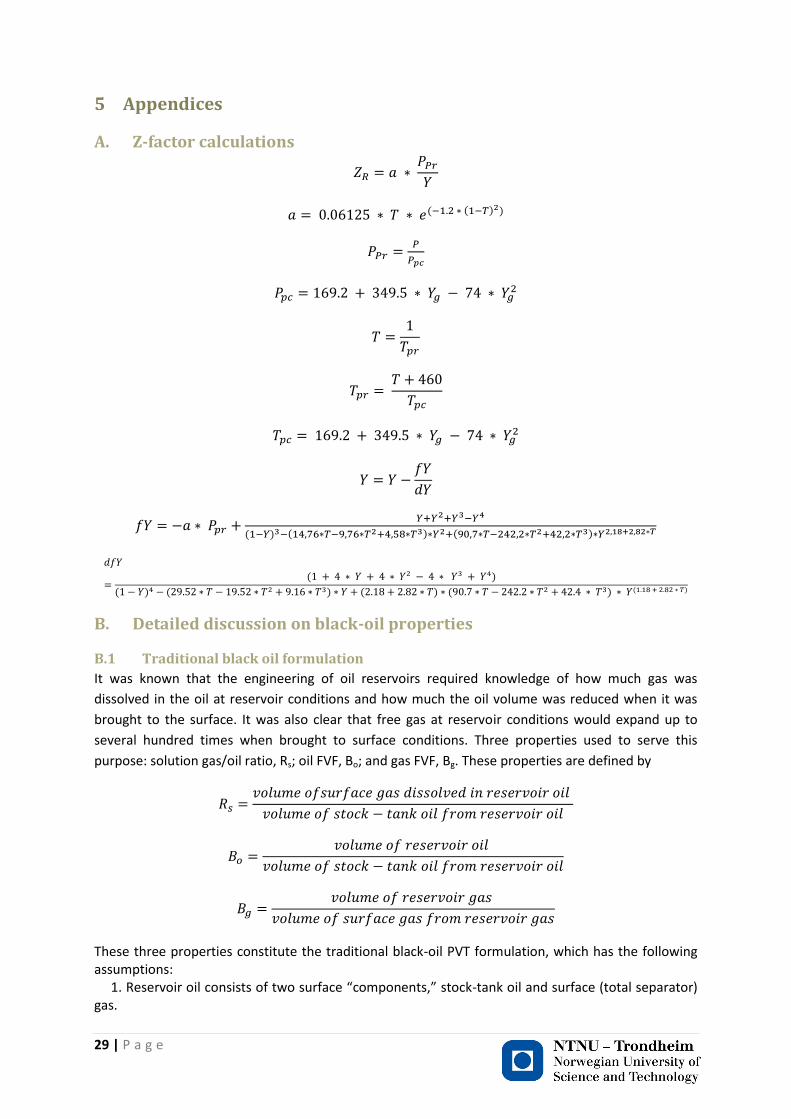
A. Z-factor calculations

( ( ) )

( ) ( ) ( )

( )

( ) ( ) ( ) ( ) ( )

B. Detailed discussion on black-oil properties

B.1 Traditional black oil formulation

It was known that the engineering of oil reservoirs required knowledge of how much gas was

dissolved in the oil at reservoir conditions and how much the oil volume was reduced when it was

brought to the surface. It was also clear that free gas at reservoir conditions would expand up to

several hundred times when brought to surface conditions. Three properties used to serve this

purpose: solution gas/oil ratio, Rs; oil FVF, Bo; and gas FVF, Bg. These properties are defined by

These three properties constitute the traditional black-oil PVT formulation, which has the following assumptions: 1. Reservoir oil consists of two surface “components,” stock-tank oil and surface (total separator) gas.

30 | P a g e

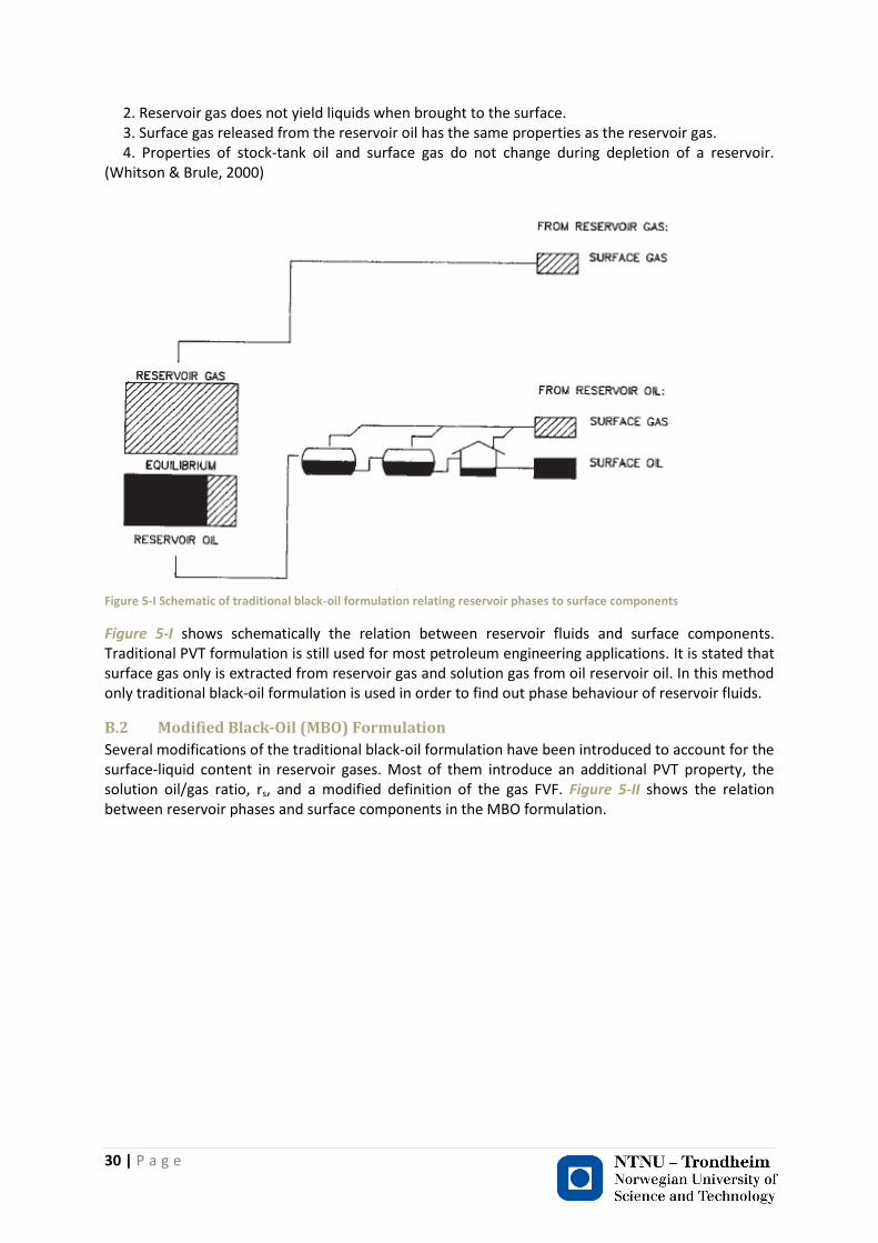
2. Reservoir gas does not yield liquids when brought to the surface. 3. Surface gas released from the reservoir oil has the same properties as the reservoir gas. 4. Properties of stock-tank oil and surface gas do not change during depletion of a reservoir. (Whitson & Brule, 2000)

Figure 5-I Schematic of traditional black-oil formulation relating reservoir phases to surface components

Figure 5-I shows schematically the relation between reservoir fluids and surface components. Traditional PVT formulation is still used for most petroleum engineering applications. It is stated that surface gas only is extracted from reservoir gas and solution gas from oil reservoir oil. In this method only traditional black-oil formulation is used in order to find out phase behaviour of reservoir fluids.

B.2 Modified Black-Oil (MBO) Formulation

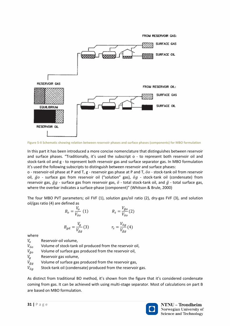
Several modifications of the traditional black-oil formulation have been introduced to account for the surface-liquid content in reservoir gases. Most of them introduce an additional PVT property, the solution oil/gas ratio, rs, and a modified definition of the gas FVF. Figure 5-II shows the relation between reservoir phases and surface components in the MBO formulation.

31 | P a g e

Figure 5-II Schematic showing relation between reservoir phases and surface phases (components) for MBO formulation

In this part it has been introduced a more concise nomenclature that distinguishes between reservoir and surface phases. “Traditionally, it’s used the subscript o - to represent both reservoir oil and stock-tank oil and g - to represent both reservoir gas and surface separator gas. In MBO formulation it’s used the following subscripts to distinguish between reservoir and surface phases: o - reservoir-oil phase at P and T, g - reservoir gas phase at P and T, - stock-tank oil from reservoir oil, - surface gas from reservoir oil (“solution” gas), - stock-tank oil (condensate) from reservoir gas, - surface gas from reservoir gas, - total stock-tank oil, and - total surface gas, where the overbar indicates a surface-phase (component)” (Whitson & Brule, 2000) The four MBO PVT parameters; oil FVF (1), solution gas/oil ratio (2), dry-gas FVF (3), and solution oil/gas ratio (4) are defined as

( )

( )

( )

( )

where Reservoir-oil volume, Volume of stock-tank oil produced from the reservoir oil, Volume of surface gas produced from the reservoir oil,

Reservoir gas volume,

Volume of surface gas produced from the reservoir gas,

Stock-tank oil (condensate) produced from the reservoir gas.

As distinct from traditional BO method, it’s shown from the figure that it’s considered condensate

coming from gas. It can be achieved with using multi-stage separator. Most of calculations on part B

are based on MBO formulation.

32 | P a g e

B.3 Surface gravities

When a well produces both oil and gas, the composite surface gravities, and , will be an average

of the surface gravities of the two reservoir phases, and for the reservoir oil and and

for the reservoir gas. The average gas gravity is given by

( ) ( )

( )

The average stock-tank-oil gravity is given by

( ) ( )

( )

where Fraction of total surface gas produced from the reservoir gas

Fraction of total stock-tank oil that comes from the reservoir oil Compositions of reservoir oil and gas change during pressure depletion, the surface gravities also vary with pressure. Surface gravities are determined separately for the reservoir-oil and reservoir-gas phases from multistage-separator calculations. In our calculation it has been done on HYSYS programing with making model.

B.4 Reservoir Material Balance – MBO PVT

As distinct from Part A, where it has been assumed that only dry gas is coming from the gas reservoir, in part B it has been considered both dry gas and gas condensate from gas reservoir. Reservoir material-balance relations for solution-gas-drive and dry-gas reservoirs are well known and widely used. In this section, reservoir material balance based on MBO properties that can be used for black oils and gas condensates. “The basis of calculation is 1bbl reservoir bulk volume. The conservation-of-mass equations for

single-cell material balance yields the following difference equations for reservoir-oil and –gas phases

during the time step with a change in average pressure from ( ) to ( ) .”

(Whitson & Brule, 2000).

In these calculations one time step equals one year.

( ) ( ) ( ) and ( ) ( ) ( )

Where and incremental quantities of total surface oil and total surface gas, respectively,

produced during the timestep;

[ ( )

] ( )

and

33 | P a g e

[

( )

] ( )

and are in STB/bbl, and are in scf/bbl, and are in scf/bbl, is in scf/STB, is in

STB/scf, and is in / scf. Other quantities used in the material-balance procedure are

( )

( )

( )

where equals oil and solution gas expansion terms and Eg is gas cap expansion terms.

The purpose of these calculations are to find out that whether there is any significant effect of using

dry-gas basis assumption or not, which has been done in the first part of our model. Application of

these relations for gas-condensate reservoirs is shown step by step.

1. Specify ( ) , total surface gas produced in scf/bbl of bulk volume.

2. Assume ( ) and calculate PVT properties and porosity (Table 4 and Table 5):

( ) ( ) ( ) (

) ( ) ( ) ( ) (

) and ( )

3. Calculate oil saturation ( ) :

( ) ( ) ( )

[ ( ) ⁄ ]

[ ( ⁄

)]

4. Calculate ( ⁄ ) from( ) .

5. Calculate( ) , ( ) , ( ) and ( ) .

6. Calculate incremental surface oil produced from reservoir oil, where ⁄

and [( ) ( )

]

7. Calculate , incremental total surface oil produced, where ⁄ and

[( ) ( ) ]

8. Calculate the material balance error ( ) ( )

34 | P a g e

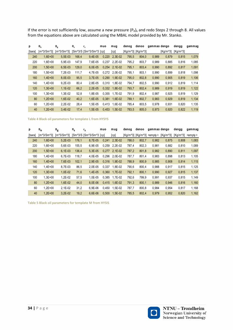
If the error is not sufficiently low, assume a new pressure (PR)k and redo Steps 2 through 8. All values from the equations above are calculated using the MBAL model provided by Mr. Stanko. p Bo Bg Rs rs muo mug denog denoo gammao dengo dengg gammag

[bara] [m^3/Sm^3] [m^3/Sm^3] [Sm^3/Sm^3][Sm^3/Sm^3] [cp] [cp] [Kg/m^3] [Kg/m^3] [Kg/m^3] [Kg/m^3]

240 1,6E+00 5,5E-03 168,4 9,4E-05 0,220 2,3E-02 795,5 804,0 0,989 0,879 0,815 1,079

220 1,6E+00 5,9E-03 147,9 7,6E-05 0,237 2,2E-02 795,2 803,7 0,989 0,885 0,816 1,085

200 1,5E+00 6,5E-03 129,0 6,0E-05 0,254 2,1E-02 795,1 803,4 0,990 0,892 0,817 1,091

180 1,5E+00 7,2E-03 111,7 4,7E-05 0,272 2,0E-02 795,1 803,1 0,990 0,899 0,818 1,098

160 1,4E+00 8,0E-03 95,5 3,7E-05 0,290 1,9E-02 795,0 802,8 0,990 0,905 0,819 1,106

140 1,4E+00 9,2E-03 80,4 2,8E-05 0,310 1,8E-02 794,7 802,5 0,990 0,912 0,819 1,114

120 1,3E+00 1,1E-02 66,2 2,2E-05 0,332 1,8E-02 793,7 802,4 0,989 0,919 0,819 1,122

100 1,3E+00 1,3E-02 52,8 1,8E-05 0,355 1,7E-02 791,9 802,4 0,987 0,925 0,819 1,129

80 1,2E+00 1,6E-02 40,2 1,6E-05 0,381 1,6E-02 789,1 802,7 0,983 0,929 0,819 1,134

60 1,2E+00 2,2E-02 28,4 1,5E-05 0,413 1,6E-02 785,4 803,5 0,978 0,931 0,820 1,135

40 1,2E+00 3,4E-02 17,4 1,5E-05 0,453 1,5E-02 783,5 805,0 0,973 0,920 0,822 1,119

Table 4 Black oil parameters for template L from HYSYS

p Bo Bg Rs rs muo mug denog denoo gammao dengo dengg gammag

[bara] [m^3/Sm^3] [m^3/Sm^3] [Sm^3/Sm^3][Sm^3/Sm^3] [cp] [cp] [Kg/m^3] [Kg/m^3] <empty > [Kg/m^3] [Kg/m^3] <empty >

240 1,6E+00 5,2E-03 176,1 8,7E-05 0,241 2,3E-02 788,0 802,7 0,982 0,875 0,808 1,083

220 1,6E+00 5,6E-03 155,5 6,9E-05 0,259 2,2E-02 787,4 802,3 0,981 0,882 0,810 1,089

200 1,5E+00 6,1E-03 136,4 5,3E-05 0,277 2,1E-02 787,2 801,8 0,982 0,890 0,811 1,097

180 1,4E+00 6,7E-03 118,7 4,0E-05 0,296 2,0E-02 787,7 801,4 0,983 0,898 0,813 1,105

160 1,4E+00 7,6E-03 102,1 2,9E-05 0,316 1,9E-02 788,9 800,9 0,985 0,908 0,814 1,115

140 1,4E+00 8,7E-03 86,5 2,0E-05 0,337 1,8E-02 790,6 800,4 0,988 0,917 0,815 1,125

120 1,3E+00 1,0E-02 71,6 1,4E-05 0,360 1,7E-02 792,1 800,1 0,990 0,927 0,815 1,137

100 1,3E+00 1,2E-02 57,5 1,0E-05 0,385 1,7E-02 792,6 799,9 0,991 0,937 0,815 1,149

80 1,2E+00 1,6E-02 44,0 8,0E-06 0,415 1,6E-02 791,3 800,1 0,989 0,946 0,816 1,160

60 1,2E+00 2,1E-02 31,2 6,9E-06 0,450 1,5E-02 787,7 800,8 0,984 0,954 0,817 1,168

40 1,2E+00 3,2E-02 19,2 6,6E-06 0,500 1,5E-02 785,5 802,4 0,979 0,952 0,820 1,162

Table 5 Black oil parameters for template M from HYSIS

35 | P a g e

6 References Det Norske Veritas. (2008). Technical Challenges and Production Forecast for Subsea Compression

System. Offshore Technology Conference, (p. 9). Houston, Texas.

Igunnu, E. T., & Chen, G. Z. (2012). Produced water treatment technologies. International Journal of

Low-Carbon Technologies, 1-21.

Norges Bank. (2013). Retrieved April 20, 2013, from www.norges-bank.no/en/price-

stability/exchange-rates/usd/aar

Statoil. (2013, January 23). Gullfaks Village 2013 NTNU - Experts in Team (EiT). Trondheim.

Store Norske Leksikon. (n.d.). Retrieved April 22, 2013, from Store Norske Leksikon:

http://www.snl.no/Gullfaks

Whitson, C. H., & Brule, M. R. (2000). Phase Behavior. Society of Petroleum.