EVALUATION OF THE AGRICULTURAL FIELD SCALE IRRIGATION REQUIREMENT SIMULATION (AFSIRS) IN PREDICTING GOLF COURSE IRRIGATION REQUIREMENTS WITH SITE-SPECIFIC DATA By MARK W. MITCHELL A THESIS PRESENTED TO THE GRADUATE SCHOOL OF THE UNIVERSITY OF FLORIDA IN PARTIAL FULFILLMENT OF THE REQUIREMENTS FOR THE DEGREE OF MASTER OF SCIENCE UNIVERSITY OF FLORIDA 2004

Welcome message from author
This document is posted to help you gain knowledge. Please leave a comment to let me know what you think about it! Share it to your friends and learn new things together.
Transcript
EVALUATION OF THE AGRICULTURAL FIELD SCALE IRRIGATION
REQUIREMENT SIMULATION (AFSIRS) IN PREDICTING GOLF COURSE IRRIGATION REQUIREMENTS WITH SITE-SPECIFIC DATA
By
MARK W. MITCHELL
A THESIS PRESENTED TO THE GRADUATE SCHOOL OF THE UNIVERSITY OF FLORIDA IN PARTIAL FULFILLMENT
OF THE REQUIREMENTS FOR THE DEGREE OF MASTER OF SCIENCE
UNIVERSITY OF FLORIDA
2004

ACKNOWLEDGMENTS
I would like to thank Dr. Grady Miller, chair of my committee, for his support and
confidence in me to complete this work. I am also thankful for the help that my other
committee member, Dr. Michael Dukes, provided me.
Also I must thank Dr. Jennifer Jacobs for her technical support with the AFSIRS
model. Special thanks go to Jan Weinbrecht and Nick Pressler, for their help and
suggestions during this research.
I would like to thank the St. Johns River Water Management District for funding
this research. I am also grateful for the encouragement from my parents and my future
wife, Sandra Buckley.
ii

TABLE OF CONTENTS page ACKNOWLEDGMENTS .................................................................................................. ii
LIST OF TABLES...............................................................................................................v
LIST OF FIGURES ........................................................................................................... vi
ABSTRACT...................................................................................................................... vii
CHAPTER
1 INTRODUCTION ........................................................................................................1
2 LITERATURE REVIEW .............................................................................................3
Golf Course Water Consumption .................................................................................3 Consumptive Use Permitting........................................................................................5 Agricultural Field Scale Irrigation Requirement Simulation (AFSIRS) ......................7
Modeling Crop Irrigation Requirements ...............................................................7 Evapotranspiration and Weather Data Inputs........................................................8 Crop Coefficient Inputs .......................................................................................12 Irrigation Application Efficiency and Uniformity Inputs....................................13 Rooting Depth Inputs ..........................................................................................14 Soil Type Inputs ..................................................................................................15
Sensitivity Analysis ....................................................................................................15 3 PREDICTING IRRIGATION REQUIREMENTS ON GOLF COURSES USING
THE AGRICULTURAL FIELD SCALE IRRIGATION REQUIREMENT SIMULATION (AFSIRS) ..........................................................................................17
Introduction.................................................................................................................17 Materials and Methods ...............................................................................................18 Results and Discussion ...............................................................................................22
Default Values .....................................................................................................22 Updated/Actual Values........................................................................................23 Default Versus Updated/Actual Irrigation Requirements ...................................25
Conclusions.................................................................................................................29
iii

4 SENSITIVITY ANALYSIS OF THE AGRICULTURAL FIELD SCALE IRRIGATION REQUIREMENT SIMULATION (AFSIRS) AND THE FAO 56 PENMAN-MONTEITH EQUATION........................................................................35
Introduction.................................................................................................................35 Materials and Methods ...............................................................................................36
Agricultural Field Scale Irrigation Requirement Simulation (AFSIRS) .............36 FAO 56 Penman-Monteith Equation...................................................................37
Results and Discussion ...............................................................................................38 Agricultural Field Scale Irrigation Requirement (AFSIRS) Sensitivity
Analysis............................................................................................................38 FAO 56 Penman-Monteith Equation Sensitivity Analysis..................................39
Conclusions.................................................................................................................39 5 SUMMARY AND CONCLUSIONS.........................................................................43
APPENDIX SAS PROGRAMS .......................................................................................45
REFERENCES ..................................................................................................................47
BIOGRAPHICAL SKETCH .............................................................................................51
iv

LIST OF TABLES
Table page 3-1 Soil types and average water contents for the five golf courses, average water
content of all soil types in the model database, and average water content of a USGA green .............................................................................................................31
3-2 Mean squares for the analysis of variance on rooting depths as influenced by golf course, location within golf course, and month ................................................31
3-3 Mean rainfall, reference ET, estimated mean irrigation requirement, irrigation requirement issued on consumptive use permit, mean irrigation requirement using updated/actual data, and applied irrigation.....................................................31
v

LIST OF FIGURES
Figure page 3-1 Yearly average reference ET (A) and rainfall (B) for the 20 year historical
weather dataset (Orlando), and for the one year of on-site weather data from each of the five golf courses.....................................................................................32
3-2 AFSIRS predicted irrigation requirements (IRR) for five golf courses. Default: model run with all default data.................................................................................33
3-3 AFSIRS predicted irrigation requirements (IRR) for three golf greens built with USGA greens mix (sand and peat). ..........................................................................34
4-1 Sensitivity analysis of the AFSIRS model output ....................................................41
4-2 Sensitivity analysis of the FAO 56 Penman-Monteith equation ..............................42
vi
Abstract of Thesis Presented to the Graduate School of the University of Florida in Partial Fulfillment of the
Requirements for the Degree of Master of Science
EVALUATION OF THE AGRICULTURAL FIELD SCALE IRRIGATION REQUIREMENT SIMULATION (AFSIRS) IN PREDICTING GOLF COURSE
IRRIGATION REQUIREMENTS WITH SITE-SPECIFIC DATA
By
Mark W. Mitchell
December 2004
Chairman: Grady L. Miller Major Department: Horticultural Sciences
Golf courses are often the focus when it comes to water use. Various water-use
models are used by Florida’s five Water Management Districts, including the
Agricultural Field Scale Irrigation Requirement Simulation (AFSIRS), to estimate
irrigation requirements on golf courses. The St. Johns River, South Florida, and North
Florida Water Management Districts use the AFSIRS model with available default data to
predict irrigation requirements for all golf courses in their jurisdiction. Default values are
used because of the limited research on golf course irrigation requirements. In this study,
data were collected at five golf courses in the Central Florida area to use in the AFSIRS
model for comparisons to irrigation requirements made using default data. Irrigation
system distribution uniformity (DULQ), rooting depths, and weather data were collected
from each golf course. Updated crop coefficients (Kc) for turfgrass were used in place of
the default values. Average soil water content for a green built to USGA specifications
vii

was used for golf courses with these types of greens, instead of the native soil average
water content. A sensitivity analysis was used to determine which inputs had the greatest
influence on the model outputs. When actual data were used, the predicted irrigation
requirements increased between 15 and 46 cm (6 and 18 in) per year for the golf courses.
Distribution uniformity had the greatest impact on predicted irrigation requirements.
When only distribution uniformities were substituted for the default irrigation system
efficiency, the irrigation requirement increased between 13 and 76 cm (5 and 30 in) per
year. Because of a limited length of actual on-site weather data, and unusually high
rainfall amounts during the year, it was difficult to use actual weather datasets in place of
the 20-year historical datasets available to the model. Sensitivity analysis further
indicated that DULQ inputs have the greatest influence on the predicted irrigation
requirements made by the AFSIRS model. Changing a DULQ from 40 to 80% (a 100%
increase) resulted in a 65% decrease in irrigation requirement. The sensitivity analysis
also showed that daily maximum temperature and mean solar radiation had the largest
impact on reference evapotranspiration rates (ETo) calculated using the FAO 56 Penman-
Monteith equation in the REF-ET program (computer program used to calculate ETo
from meteorological data). A 25% increase in the starting point for maximum
temperature resulted in a 45% increase in ETo, and a 50% increase of the starting point
for mean solar radiation results in a 33% change in ETo. Using actual data in place of
default values in the AFSIRS model can result in site-specific estimates of irrigation
requirements on golf courses. According to the AFSIRS model, and further illustrated
through sensitivity analysis, DULQ and Kc values had the greatest impact on irrigation
requirements. Therefore, these variables need to be measured with the most accuracy.
viii

CHAPTER 1 INTRODUCTION
In recent years, golf has become popular in the United States. There were over
15,000 golf facilities in the country in 2000, and over 1,100 courses located in Florida
(National Golf Foundation, 2004). Because of the number of golf courses in Florida, and
their visibility, there is a public concern that the golf industry wastes water. Because of
Florida’s erratic distribution of rainfall and large extent of sandy soils, irrigation is
necessary to maintain quality turfgrass.
Water use in Florida is controlled by five Water Management Districts. Each
District is responsible for issuing consumptive use permits to large water users (including
golf courses) located in their jurisdiction. These permits allocate the maximum amount of
water a golf course should use per year. A golf course is required to report these water
use amounts yearly; and if the allotment is exceeded, a financial penalty may be issued by
the District.
The Water Management Districts use various mathematical models to determine
crop irrigation requirements. The St. Johns River Water Management District
(SJRWMD), South Florida Water Management District, and North Florida Water
Management District use the Agricultural Field Scale Irrigation Requirement Simulation
(AFSIRS) to estimate crop water needs, including turfgrass. The AFSIRS model was
developed at the University of Florida, and is a numerical simulation model that estimates
irrigation requirements for Florida crops, soils, irrigation systems, climate conditions, and
irrigation management practices (Smajstrla, 1990). Historical (default) datasets are
1

2
available to the model for crop (turfgrass) coefficient values, rooting depths, irrigation
system efficiencies, soil water capacities, rainfall, and reference evapotranspiration rates.
Because the SJRWMD uses the default data when determining irrigation requirements for
golf courses, the allotment amounts are not site-specific to each golf course in their
jurisdiction.
Because of limited research on golf course irrigation requirements, there were two
objectives to this research. The first objective was to compare AFSIRS water requirement
estimates made with default data to estimates made with actual data collected from golf
courses. The second objective was to determine what model inputs have the greatest
influence on outputs, in order to ascertain the variables that should be measured and
monitored to the greatest extent.

CHAPTER 2 LITERATURE REVIEW
Golf Course Water Consumption
Total water use by Florida golf courses in 2000 was estimated at 650 billion liters
(172 billion gal) (Haydu and Hodges, 2002). According to this survey, nearly 321 billion
liters (85 billion gal) came from recycled water, 185 billion liters (49 billion gal) from
surface water, 132 billion liters (35 billion gal) from on-site wells, and 5.7 billion liters
(1.5 billion gal) from municipal sources. It was estimated that the average water use per
golf course was 503 million liters (133 million gal) per year.
Golf courses receive water allotments from water management districts based on
total irrigated acreage; but courses consist of areas managed with varying levels of inputs,
and areas that often require different amounts of water. Greens (areas prepared for
putting) usually receive the most maintenance, followed by the tees (areas prepared for
playing the first shot of each hole); fairways (turfed areas between tees and greens); and
rough (turfed area surrounding the greens, tees, and fairways) (Beard, 2002). The amount
of water these areas require depends on the type of grass, rooting depth, soil type,
maintenance level, amount of inputs, and the desired effect.
A traditional golf course has 4 par 3-holes, 4 par 5-holes, and 10 par 4-holes, which
occupy approximately 54 hectares (133 acres) (McCarty et al., 2001). Tees take up 0.16
to 1.2 hectares (0.4 to 3 acres) of a golf course (McCarty et al., 2001). Par 4 and par 5
tees typically occupy 9.3 to 18.6 m2 (100 to 200 ft 2 ), and par 3 tees range from 18.6 to
33.2 m2 (200 to 357 ft 2 ) per thousand rounds of golf annually (Beard, 1985). Greens
3

4
typically range from 465 to 697 m2 (5,000 to 7,500 ft 2 ) in size, and occupy 0.85 to 1.33
hectares (2.1 to 3.3 acres) on a typical 18-hole golf course (Beard, 2002).
Fairways comprise 12 to 24 hectares (30 to 60 acres) on a golf course (Beard,
1985). The average size of a fairway (the turfed area between the tee and green) is
approximately 1.2 hectares (3 acres), which is dependent on the playing length of the hole
and the width of the fairway. The usual fairway width on a golf course is approximately
32 meters (35 yards) (Beard, 2002). Depending on the total acreage and design of the
course, the rough can range from 26 to 49 hectares (65 to 120 acres) for a golf course
(Beard, 2002).
Approximately 26% of the total acreage of a golf course is considered fairways and
55% is rough. Therefore, most water use on a golf course occurs in irrigating fairways
and rough, and increasing and decreasing the total area of these zones can have a great
impact on the amount of water use on a golf course.
In the past, golf courses were built using only the existing soil at the construction
site. Greens were built by pushing up the soil, in order to promote runoff of water (Beard,
1982). Fairways and roughs are still generally built using available soil on site, but to
construct some surface features, soil may be excavated. Therefore, fairways or rough may
be established using subsoil, which usually has different soil characteristics than surface
soil layers. Because the subsoil may have a different water-holding capacity than the
surface soil, water requirements can differ in areas where subsoil was used.
Although some golf courses still have push-up greens, most newly constructed or
renovated greens have been built to United States Golf Association (USGA) green
specifications. The profile of a USGA green consists of 30 to 36 cm (12 to 14 in) of

5
rootzone medium (fine textured) above a 5 to 10 cm (2 to 4 in) coarse sand layer (choker
layer) covering a 10 cm (4 in) layer of gravel (Higgins and McCarty, 2001). Drainage
tile is installed underneath the gravel layer, in a herringbone design. This design allows
for the entire rootzone to reach field capacity before water drains through the gravel layer
and into the drainage tile. Field capacity is the percentage of water that remains in the soil
after having been saturated and after free drainage has practically ceased (Brady and
Weil, 1999). The field capacity of a USGA greens mix should be in the range of 0.16 to
0.33 m3 m-3 (Beard, 2002).
Consumptive Use Permitting
Florida has five Water Management Districts that regulate water control and use.
The Districts’ main responsibilities include management of water and related land
resources; proper use of surface and groundwater resources; regulation of dams,
impoundments, reservoirs, and other structures to alter surface water movement;
combating damage from floods, soil erosion, and excessive drainage; developing water
management plans; maintenance of navigable rivers and harbors, participation in flood
control programs; and maintaining water management and use facilities (Olexa et al.,
1998). Each District is run by a governing board consisting of nine members. The
members serve 4-year terms, and are appointed by the governor and confirmed by the
state. Generally, an executive director is responsible for the operation of the District,
including the implementation of policies and rules (Olexa et al., 1998).
Florida’s Water Management Districts issue several types of water use permits, the
most common being consumptive use permits (CUPs). A CUP authorizes how much
water should be withdrawn from surface and ground water supplies for reasonable and
beneficial uses such as public supply (drinking water), agricultural and landscape

6
irrigation, industry, and power generation (SJRWMD, 2004). The water withdraw
situations that require a CUP are: a well that measures 15.2 mm (6 in) or more in
diameter, the annual average is more than 378,500 liters (100,000 gal) of water use per
day, or there is the capacity to pump 3.78 million liters (1 million gal) or more of water
per day (SJRWMD, 2004).
The St. Johns River Water Management District (SJRWMD) began issuing
consumptive use permits (CUPs) in 1983. The District covers parts of Central Florida and
the Northeast portion of the state. Since 1991, all permitted users have been required to
report their water use by using a meter or by an alternative method approved by the
District. In the year 2000, 504 CUPs were issued by the District (SJRWMD, 2004).
To receive a CUP, an applicant must submit an application form, along with a fee,
a listing of adjacent property owners, and a water conservation plan which provides
measures to reduce water use and preserve water resources for other beneficial uses. The
District then reviews the application and determines the allotment duration and amount
(SJRWMD, 2002). The permits are issued for approximately 20 years, and upon
expiration, must be renewed. CUPs for golf courses are usually issued for a shorter period
of time because of changes that are often made to courses such as adding golf holes, or
changing water sources.
The factors that cause the difference in water allotments from golf course to golf
course are total irrigated acreage and soil type. The applicant reports the irrigated
acreage on the CUP application, and the District uses existing soil maps to determine the
soil type at the location where the golf course was built. Golf courses may use different
sources of water such as: wells, lakes, and reclaimed water, but the total amount

7
withdrawn from all sources must not exceed their CUP amount. During water shortages,
the district may impose restrictions, and these restrictions supersede any conditions of the
permit (SJRWMD, 2002).
Agricultural Field Scale Irrigation Requirement Simulation (AFSIRS)
Modeling Crop Irrigation Requirements
When determining the amount of water to issue on a consumptive use permit, the
Water Management District must predict the irrigation requirement for the crop.
Irrigation requirement (IRR) for a crop is the amount of water, in addition to rainfall, that
must be applied to meet a crop’s evapotranspiration needs without significant reduction
in yield (Smajstrla and Zazueta, 1998). In terms of golf course turfgrass, quality must not
be significantly reduced. Evapotranspiration (ET) includes water that is needed for both
evaporation and transpiration. The amount of water issued on the CUP for a golf course is
determined by predicting the IRR for the turfgrass on that course and any other area that
may be irrigated on or around the course, e.g. home landscapes.
Estimates of IRRs can be ascertained from historical observation, or by using
numerical models (Smajstrla and Zazueta, 1998). If a long term record has been kept of
irrigation water applied, this record could be used to estimate future uses. But few such
long-term databases exist. Another problem with historical data is that its use may be
limited to the location where it was collected (Smajstrla and Zazueta, 1998). The effects
of differences in climate, soil, location, time of year during which the crop was grown, as
well as other factors on irrigation requirements cannot be determined from the available
data (Smajstrla and Zazueta, 1998).
Numerical models may be based on statistical methods or on physical laws which
govern crop water uptake and use (Smajstrla and Zazueta, 1998). A basic model that has

8
been used is The Soil Conservation Service (SCS) procedure (SCS, 1970). This model is
a statistical regression method that allows monthly crop irrigation requirements to be
estimated based on three factors: monthly crop ET, monthly rainfall, and soil water-
holding characteristics (SCS, 1970). Limitations of this model are: estimation of
irrigation requirements for monthly or longer time periods only, that it is limited to
sprinkler and surface irrigation systems which irrigate the entire soil surface, and soil
types with deep water tables (SCS, 1970).
The SJRWMD uses the Agricultural Field Scale Irrigation Requirement Simulation
(AFSIRS) model to predict IRR for a crop (SJRWMD, 2004). The AFSIRS model is a
numerical simulation model which estimates IRR using inputs from Florida crops, soils,
irrigation systems, growing seasons, climate conditions, and irrigation management
practices (Smajstrla, 1990). This model is based on a water budget of the crop root zone.
This water budget includes inputs to the crop root zone from rain and irrigation, and
losses from the root zone by drainage and evapotranspiration. The water holding capacity
in the crop root zone is the multiple of the water-holding capacity of the soil and the
rooting depth of the crop being irrigated (Smajsrla, 1990).
Evapotranspiration and Weather Data Inputs
The AFSIRS model is based on the concept that actual crop ET is estimated from
reference ET and crop water use coefficients. Reference evapotranspiration (ETo) is the
rate of evapotranspiration from an extensive surface of 8 to 15 cm tall, green grass cover
of uniform height, which is actively growing, completely shading the ground and not
lacking water (Allen et al., 1998). A crop coefficient (Kc) is an adjustment factor which
is determined by different crop characteristics, i.e. turfgrass type, quality, and height
(Brown and Kopec, 2000). Daily ETo, as well as rainfall, can be ascertained from

9
historical climate data available in the model. Records from nine Florida locations over
approximately a 20 year period ending in the 1970s are part of the AFSIRS model
database (Smajstrla, 1990). AFSIRS computes IRR for the mean year over those 20 years
as well as IRR for different probabilities of occurrence. The SJRWMD permits are based
on an 80% probability of occurrence, which means that the permittee, or golf course,
should not exceed their allotment except for a 2 in 10 year drought (V. McDaniel,
personal communication, 2004).
There are many weather station networks that can be used by agricultural growers
and turfgrass managers to determine ETo (Brown et al., 2001). The California Irrigation
Information System (CIMIS) (Snyder, 1986) is an integrated network of over 120
computerized weather stations located throughout California. The Arizona
Meteorological Network (AZMET) provides weather-based information in southern and
central Arizona (Brown et al., 1988). These networks use the modified Penman equation
to determine ETo. The commonly used modified Penman and modified Penman-Monteith
methods are two of the many mathematical models that compute ETo from measured
weather data (Brown and Kopec, 2000). The Florida Automated Weather Network
(FAWN) consists of 30 weather stations located throughout Florida. These stations
collect data that can be use for determining ETo (FAWN, 2004). The common data
collected daily by a weather station for computing ETo are: minimum and maximum
temperature, minimum and maximum relative humidity, mean solar radiation, and mean
wind speed.
There are computer programs, such as REF-ET, that can calculate ETo from
meteorological data using different mathematical models, including the commonly used

10
modified Penman-Monteith method. REF-ET is a stand-alone computer program that
calculates ETo from meteorological data made available by the user (Allen, 2002). The
program provides standardized calculations of ETo for fifteen of the more common
mathematical models that are currently in use in the United States and Europe (Allen,
2002). Daily ETo values in the AFSIRS database were calculated using the IFAS Penman
equation (Smajstrla, 1990). The IFAS Penman was developed at the University of
Florida’s Institute of Food and Agricultural Sciences in 1984 to better represent regional
climatic tendencies. The Penman formula is based on four major climatic factors: net
radiation, air temperature, and wind speed and vapor pressure deficit (Jacobs and Satti,
2001).
( ) ( )λ
σαγ
−−−−
+∆∆
=
42.042.108.056.01 4
so
sds
o
RR
eTRET (2-1)
( )([ ]da eeu −++∆
+ 20062.05.0263.0γ
)γ
where: ETo Reference evapotranspiration (mm day-1) ∆ Slope of saturated vapor pressure curve of air (mb/oC) γ Psychometric constant (0.66 mb/oC) α Albedo or reflectivity of surface for Rs Rs Total incoming solar radiation (cal. cm-2 day-1) σ Stefan-Boltzmann constant (11.71 x 10⁻⁸ cal.cm-2 day-1 K-1) T Average air temperature (K) ed vapor pressure at dewpoint temperature (mb) Rso Total daily cloudless sky radiation (cal cm-2 day-1) u2 wind speed at a height of 2 m (km day-1) ea vapor pressure of air (mb) Jacobs and Satti (2001) reported that the IFAS Penman equation is not as consistent
as the FAO 56 Penman-Monteith (Allen et al.,1998) equation for Florida conditions. In
their study, fourteen models that may be used to estimate ETo in consumptive use

11
permitting were reviewed to identify the approaches that: best represented the physics of
water losses from irrigated crops; easiest to use in terms of parameters needed; were able
to consistently and accurately capture ETo losses in growing regions of Florida; and were
considered acceptable to the general scientific community. Jacobs and Satti (2001)
suggested that the ETo data available to the AFSIRS should be updated with newer
weather data using the FAO 56 Penman-Monteith equation (Allen et al., 1998).
( ) ( )( )2
2
34.01273
900408.0
u
eeuT
GRET
asn
o ++∆
−+
+−∆=
γ
γ (2-2)
where: ETo Reference evapotranspiration (mm day-1) ∆ Slope of saturation vapor pressure temp. relationship (KPa oC-1) Rn Net radiation (MJ m-2 day-1) G Soil heat flux (MJ m-2 day-1, generally assumed to be zero) γ Psychometric constant (KPa oC-1) T Average air temperature (oC) u2 wind speed at a height of 2 m (m s-1) es saturation vapor pressure (KPa) ea actual vapor pressure (KPa) Turf ET rates can vary among genotypes as well as region to region. Carrow (1995)
reported that ET rates for cool season grasses ranged from 1.99 - 6.05 mm d-1 and warm
season grasses varied from 1.40 - 6.22 mm d-1. ‘Tifway’ bermudagrass [Cynodon
dactylon L. x C. transvaalensis Burt-Davy], the most common grass grown on Florida
golf courses, had an average summer ET rate of 3.11 mm d-1 in Central Georgia (Carrow,
1995). Beard et al. (1992) reported summer averages of 5.10 mm d-1 for the same
genotype in the arid west.
Studies have indicated that turf ET increases with water availability. According to
Kneebone and Pepper (1982), ET rates of bermudagrass [Cynodon dactylon (L.)]
increased with increased irrigation application rates and increased water-holding

12
capacities of soils. Also, turf ET rates increased with increased light levels, increased
temperatures, lowered humidity, moderate to high wind speeds, and long days (Carrow,
1995).
Cultural and fertilization practices influence turf ET rates. There have been a
number of studies showing turf ET rates decrease as the cutting height was lowered (Kim
and Beard, 1983; Parr et al., 1984; Unruh et al., 1999). High rates of nitrogen have
produced an increase in shoot growth and a reduction in root growth (Beard, 1973; Goss
and Law, 1967). The reduced root growth results in less available water to the turf and
the increase in shoot growth requires more water to be taken up. Therefore, more
frequent irrigation is needed to supply enough moisture for growth (Beard, 1973).
Crop Coefficient Inputs
Crop Coefficients (Kc) are available in the AFSIRS database for 60 different crops
(Smajstrla, 1990). The Kc value in the database for golf course turf is one, and therefore
the AFSIRS computes the actual evapotranspiration rate of golf course turf being equal to
the reference evapotranspiration rate (Smajstrla, 1990). According to Jacobs and Satti
(2001), the AFSIRS model should have additional Kc values for turfgrasses because the
additional research conducted since the model was designed indicates differing turfgrass
Kc values between grasses and months. In Georgia, Carrow (1995), using the FAO
Penman, reported Kc values during the summer for Tifway bermudagrass varied from
0.53 to 0.97. Crop coefficient values for Tifway bermudagrass in Arizona, using the
Penman Monteith, ranged from 0.78 to 0.85 and intermediate ryegrass [L. hybridum]
ranged from 0.78 to 0.89 (Brown and Kopec, 2000). Because ryegrass is seeded in the
winter time in some parts of Florida as the bermudagrass goes dormant, different Kc
values within the year may need to be used for computing turf ET.
13
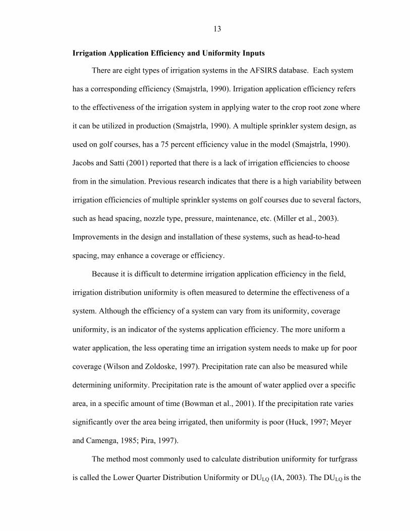
Irrigation Application Efficiency and Uniformity Inputs
There are eight types of irrigation systems in the AFSIRS database. Each system
has a corresponding efficiency (Smajstrla, 1990). Irrigation application efficiency refers
to the effectiveness of the irrigation system in applying water to the crop root zone where
it can be utilized in production (Smajstrla, 1990). A multiple sprinkler system design, as
used on golf courses, has a 75 percent efficiency value in the model (Smajstrla, 1990).
Jacobs and Satti (2001) reported that there is a lack of irrigation efficiencies to choose
from in the simulation. Previous research indicates that there is a high variability between
irrigation efficiencies of multiple sprinkler systems on golf courses due to several factors,
such as head spacing, nozzle type, pressure, maintenance, etc. (Miller et al., 2003).
Improvements in the design and installation of these systems, such as head-to-head
spacing, may enhance a coverage or efficiency.
Because it is difficult to determine irrigation application efficiency in the field,
irrigation distribution uniformity is often measured to determine the effectiveness of a
system. Although the efficiency of a system can vary from its uniformity, coverage
uniformity, is an indicator of the systems application efficiency. The more uniform a
water application, the less operating time an irrigation system needs to make up for poor
coverage (Wilson and Zoldoske, 1997). Precipitation rate can also be measured while
determining uniformity. Precipitation rate is the amount of water applied over a specific
area, in a specific amount of time (Bowman et al., 2001). If the precipitation rate varies
significantly over the area being irrigated, then uniformity is poor (Huck, 1997; Meyer
and Camenga, 1985; Pira, 1997).
The method most commonly used to calculate distribution uniformity for turfgrass
is called the Lower Quarter Distribution Uniformity or DULQ (IA, 2003). The DULQ is the

14
average water applied in the twenty-five percent of the area receiving the least amount of
water, divided by the average water applied over the entire area (IA, 2003). Pitts et al.
(1996) evaluated 385 residential irrigation systems, and reported that the average DULQ
for agricultural sprinklers, micro-irrigation, furrow irrigation and turf irrigation were 65,
70, 70, and 49 percent, respectively. Of the 37 turf irrigation systems evaluated, 40% had
DULQ’s less than 40%. Golf courses have historically had DULQ’s ranging from 55 to 85
percent (Thompson, 2002). The Irrigation Association (2003) suggests that a 70 percent
uniformity is a good (expected) value when evaluated using their methodology.
Rooting Depth Inputs
Each of the 60 crops in the AFSIRS database has irrigated (average) and maximum
rooting depth values. The model uses these values, along with soil properties, to compute
how much water needs to be applied to reach field capacity. The AFSIRS model assumes
that 70 percent of water uptake occurs in the irrigated root zone and the remaining 30
percent occurs below the irrigated root zone (Smajstrla, 1990). For golf course turfgrass,
the model uses 15 and 61 cm (6 and 24 in), irrigated and maximum rooting depths
(Smajstrla, 1990). Jacobs and Satti (2001) reported that the AFSIRS model needs
additional rooting depths for turfgrasses because rooting depths can vary from golf course
to golf course.
Beard (1973) reported that the majority of a turfgrass root system mowed regularly
at less than 5 cm, is located in the upper 7 cm of the soil. Reduced rooting depth is
directly correlated with a decrease in cutting height. The very close cutting heights
required to meet performance demands by today’s golfers, may result in shallow rooting.
There is very limited research currently available documenting effective rooting depths of
golf course turfs.
15
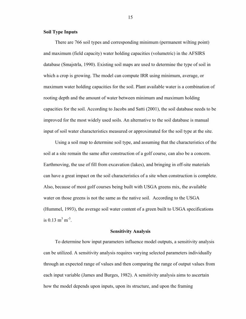
Soil Type Inputs
There are 766 soil types and corresponding minimum (permanent wilting point)
and maximum (field capacity) water holding capacities (volumetric) in the AFSIRS
database (Smajstrla, 1990). Existing soil maps are used to determine the type of soil in
which a crop is growing. The model can compute IRR using minimum, average, or
maximum water holding capacities for the soil. Plant available water is a combination of
rooting depth and the amount of water between minimum and maximum holding
capacities for the soil. According to Jacobs and Satti (2001), the soil database needs to be
improved for the most widely used soils. An alternative to the soil database is manual
input of soil water characteristics measured or approximated for the soil type at the site.
Using a soil map to determine soil type, and assuming that the characteristics of the
soil at a site remain the same after construction of a golf course, can also be a concern.
Earthmoving, the use of fill from excavation (lakes), and bringing in off-site materials
can have a great impact on the soil characteristics of a site when construction is complete.
Also, because of most golf courses being built with USGA greens mix, the available
water on those greens is not the same as the native soil. According to the USGA
(Hummel, 1993), the average soil water content of a green built to USGA specifications
is 0.13 m3 m-3.
Sensitivity Analysis
To determine how input parameters influence model outputs, a sensitivity analysis
can be utilized. A sensitivity analysis requires varying selected parameters individually
through an expected range of values and then comparing the range of output values from
each input variable (James and Burges, 1982). A sensitivity analysis aims to ascertain
how the model depends upon inputs, upon its structure, and upon the framing

16
assumptions made to build it. As a whole, sensitivity analysis is used to increase the
confidence in a model and its predictions, by providing an understanding of how the
model’s response variables respond to changes in the inputs (A forum on sensitivity
analysis, 2004).
The input parameters with the greatest influence on the model output need to be
measured with the highest accuracy. The South Florida Water Management District used
sensitivity analysis to assess the impact of parameter errors on the uncertainty in output
values for the South Florida Water Management Model and the Natural Systems Model
(Loucks and Stedinger, 1994). Engineers in the District use these models to predict
possible hydrologic impacts of alternative water management policies under a variety of
hydrologic inputs. Once the key errors were identified, it was possible to determine the
extent to which parameter uncertainty can be reduced through field investigations,
development of better models, and other efforts (Loucks and Stedinger, 1994).

CHAPTER 3 PREDICTING IRRIGATION REQUIREMENTS ON GOLF COURSES USING THE AGRICULTURAL FIELD SCALE IRRIGATION REQUIREMENT SIMULATION
(AFSIRS)
Introduction
Florida’s five Water Management Districts issue consumptive use permits to all
golf courses within their areas of jurisdiction. These permits are based on the irrigation
requirement (IRR) of the turfgrass on the golf course. Historical observations and
computer models are tools that are used to predict IRR. The St. Johns River Water
Management District (SJRWMD), South Florida Water Management District, and North
Florida Water Management District use the Agricultural Field Scale Irrigation
Requirement Simulation (AFSIRS) model to predict IRR for golf courses.
The AFSIRS model is a numerical simulation model which estimates IRR using
inputs from Florida crops, soils, irrigation systems, growing seasons, climate conditions,
and irrigation management practices (Smajstrla, 1990). This data is input into the model
from datasets that were constructed using historical data and previous research. Due to
the dependency on these datasets, there are some limitations to operational use of the
model.
The limitations specifically pertaining to golf courses were postulated during a
study at the University of Florida by Jacobs and Satti (2001). They found that the major
problem with the simulation is that it does not have the ability to input actual rainfall and
climate data from the site of interest. They also found that the mathematical model used
to calculate the reference ET rates for the datasets, the IFAS Penman Equation, is not as
17

18
consistent as the FAO 56 Penman-Monteith equation (Allen et al., 1998) for Florida
conditions.
Jacobs and Satti (2001) reported that the crop coefficient values and rooting depths
available to the model need to be updated. There has been more research conducted on
crop coefficients since the model was designed, and rooting depths can vary from golf
course to golf course. They also indicated that there is a lack of irrigation efficiency
values available to the user. Previous research indicates that there is a high variability
between distribution uniformities of multiple sprinkler systems on golf courses due to
several factors such as head spacing, nozzle type, pressure, maintenance, etc. (Miller et
al., 2003).
The AFSIRS model has a soil database which is made up of 766 soil types found in
Florida. Because most golf courses are constructed with the USGA greens mix, that has
different soil water characteristics than native Florida soils, IRR for golf course greens
can not be accurately predicted using the soil dataset. The objective of this study was to
compare AFSIRS water requirement estimates made with default data to estimates made
with actual data collected from golf courses.
Materials and Methods
Data were collected from five golf courses located in Central Florida. Irrigation
system performance data measured included distribution uniformity and precipitation
rates. Because it its extremely difficult to determine irrigation system efficiency in a field
setting, distribution uniformity values were collected and used in the model to replace the
default efficiency value. To determine irrigation distribution uniformities, irrigation
audits were performed on three golf holes at each of the five courses in March through
May 2002 (Pressler, 2003). The audits were conducted using the methods of ANSI/ASAE

19
S436.1 MAR 01 Standards (ASAE, 2001), and using the evaluation methodology
described in the Irrigation Association of America’s Certified Golf Course Irrigation
Auditor training manual (IA, 2003).
The catch-cans used in this study had an opening diameter of 7.6 cm (3.0 in) and a
depth of 10.8 cm (4.25 in). For tee complexes (all tees) and greens, catch-cans were
placed in a grid pattern on 3-m centers over the entire surface. For fairways, catch-cans
were placed in a grid pattern on 9-m centers throughout the entire fairway and primary
rough, if irrigated (Pressler, 2003).
The number of sprinklers operating at one time was representative of the normal
operating conditions of that particular system. Each location within individual courses
received the same amount irrigation runtime. The runtime on fairway and tees ranged
between 20 and 30 minutes per zone, and greens between 10 and 30 minutes per zone.
Once it was determined that all the zones had run for a certain location, the collected
water in each can was measured and recorded using a 500 mL graduated cylinder. Lower
quarter distribution uniformity (DULQ) was determined by (Pressler, 2003):
100. xV
LQAvgDUavg
LQ = (3-1)
DULQ = Lower Quarter Distribution Avg. LQ = Average volume of lowest 25% of observations Vavg = Average catch can volume For modeling purposes, an average DULQ for each of the three holes on the five
courses was determined by weighting the DULQ based on the total areas of tees, fairway,
and green. Areas were determined from global positioning system maps, produced within
60 days of uniformity testing.

20
Precipitation rates were also collected for each location on a golf course. The net
precipitation rate (PR) is the rate that sprinklers apply water to a given area per unit time
and can be calculated as follows:
60avg
net
VPR
TR CDA×
=×
(3-2)
PRnet = Net Precipitation Rate, (cm h-1) Vavg = Average catch can volume (mL) TR = Testing run time (min) CDA = Catch can opening (cm2) The precipitation rates were used to determine how much water golf courses
actually applied during the study. Those values were then compared to the IRR predicted
by the model for each golf course.
Maximum and average rooting depths were measured at three locations (tees,
fairways, and greens) at each golf course. Measurements were taken in September and
November 2002 and February and May 2003. Three random samples were taken at a 15
cm depth from each location using a Mascaro soil profiler (Turf-Tec International, Coral
Springs, FL). The maximum rooting depth was determined by physically measuring the
longest root in each of the three samples. Measurements were taken from the top of the
thatch layer to the tip of the root. These values were then averaged and the mean
maximum rooting depth of the three samples was recorded as the maximum rooting depth
for that location. Average rooting depth was determined by visually assessing the
samples where the majority of the roots were present. A ruler was then used to measure
the distance to the top of the thatch layer. These measurements were then averaged and a
mean rooting depth was calculated for each location (Pressler, 2003).

21
Weather stations were installed to monitor environmental parameters from June
2002 to May 2003. The weather stations were located in flat-grassed areas so that the
nearest obstruction was at least ten times its height away from the station. The stations
were placed in irrigated areas on the golf course property. The stations recorded the date,
time, temperature, soil heat flux, (HFT3, Radiation Energy Balance Systems, Bellevue,
WA), solar radiation (LI-200SZ, Licor Inc. Lincoln, NE), wind speed and direction
(WAS425, Vaisala, Inc., Sunnyvale, CA), relative humidity (HMP 45C, Vaisala, Inc.,
Woburn, MA), and precipitation (TE525 Tipping Bucket, Texas Electronics, Inc., Dallas
TX) at 15 minute intervals via a CR10X datalogger (Campbell Scientific, Inc., Logan
Utah).
The data collected by the weather stations was used to develop five site specific
weather datasets containing daily reference ET rates and rainfall. Reference ET (ETo)
rates were calculated using the computer program REF-ET. REF-ET was developed as a
stand-alone computer program to calculate ETo from meteorological data made available
by the user (Allen, 2002). Because the FAO 56 Penman-Monteith equation (Allen et al.,
1998) was found to be the most consistent model for determining ETo for Florida
conditions (Jacobs and Satti, 2001), this equation was used to calculate ETo for the site
specific weather datasets.
Because it is difficult to determine site-specific crop coefficients (Kc) in the field,
updated Kc values were determined from a literature review to replace the default values
in the model. Kc values for bermudagrass were determined from Carrow’s (1995) study
in Georgia, and overseeded ryegrass Kc values were determined from Brown and
Kopec’s (2000) study in Arizona.
22
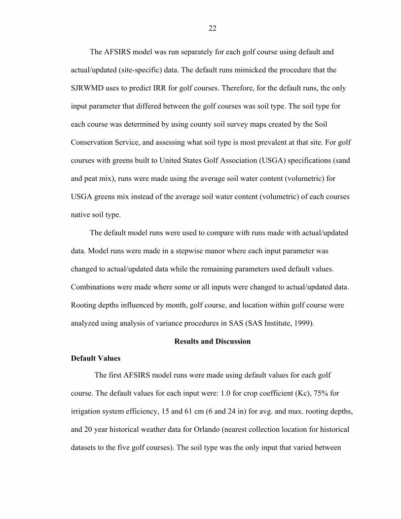
The AFSIRS model was run separately for each golf course using default and
actual/updated (site-specific) data. The default runs mimicked the procedure that the
SJRWMD uses to predict IRR for golf courses. Therefore, for the default runs, the only
input parameter that differed between the golf courses was soil type. The soil type for
each course was determined by using county soil survey maps created by the Soil
Conservation Service, and assessing what soil type is most prevalent at that site. For golf
courses with greens built to United States Golf Association (USGA) specifications (sand
and peat mix), runs were made using the average soil water content (volumetric) for
USGA greens mix instead of the average soil water content (volumetric) of each courses
native soil type.
The default model runs were used to compare with runs made with actual/updated
data. Model runs were made in a stepwise manor where each input parameter was
changed to actual/updated data while the remaining parameters used default values.
Combinations were made where some or all inputs were changed to actual/updated data.
Rooting depths influenced by month, golf course, and location within golf course were
analyzed using analysis of variance procedures in SAS (SAS Institute, 1999).
Results and Discussion
Default Values
The first AFSIRS model runs were made using default values for each golf
course. The default values for each input were: 1.0 for crop coefficient (Kc), 75% for
irrigation system efficiency, 15 and 61 cm (6 and 24 in) for avg. and max. rooting depths,
and 20 year historical weather data for Orlando (nearest collection location for historical
datasets to the five golf courses). The soil type was the only input that varied between

23
golf courses. According to the SCS county soil survey maps, three of the five courses had
the same soil type average water contents (Table 3-1).
Updated/Actual Values
Based on crop coefficient (Kc) research reported by Carrow (1995) and Brown and
Kopec (2000) on bermudagrass and ryegrass monthly crop coefficients, updated Kc
values were entered into the model for each corresponding month to replace the default
value of 1.0. Crop coefficients inputted for bermudagrass were: 0.62 in May, 0.54 in
June, 0.53 in July, 0.65 in August, 0.97 in September, and 0.73 in October. Crop
coefficients inputted for ryegrass were: 0.83 in November, 0.80 in December, 0.78 in
January, 0.79 in February, 0.86 in March, and 0.89 in April.
Measured DULQ for each golf course were used to replace the default (75%)
irrigation system efficiency for a multiple sprinkler system. An average DULQ for each of
the three holes on the five courses was determined by weighting the DULQ for each
location (tee, fairway, green) based on their total areas. Because the fairway occupies the
most area, the DULQ for a hole was similar to the DULQ of the fairway on that hole. The
weighted average DULQ’s for the three holes on the five courses were calculated as
follows: golf course A = 32, 37, and 59%, golf course B = 40, 42, and 49%, golf course C
= 45, 55 and 62%, golf course D = 62, 67, and 67%, and golf course E = 41, 44, and 54%.
Average and maximum rooting depths measured at each golf course were entered
into the model in-place of the default values of 15 and 61 cm (6 and 24 in). Because two
of the three holes on each golf course had reduced runtimes, in accordance with a
concurrent irrigation conservation study (Pressler, 2003), only the rooting depths from
the control holes (typical irrigation practices) were used for modeling. Analysis of

24
variance indicated differences in rooting depths by month at a 95% probability level
(Table 3-2).
Rooting depths measured in August, 2002 were significantly less than depths
measured in November, 2002, and February and May 2003. But because these rooting
depth differences may have been caused by the extremely wet summer in 2002, rooting
depths from each month and location were averaged together to get an average and
maximum rooting depth for each golf course. The average (irrigated) and maximum
rooting depths from the five golf courses, used for modeling, were (avg. and max.): golf
course A = 4.3 and 6.6 cm (1.7 and 2.6 in), golf course B = 4.3 and 7.1 cm (1.7 and 2.8
in), golf course C = 4.6 and 7.4 cm (1.8 and 2.9 in), golf course D = 4.6 and 6.6 cm (1.8
and 2.6 in), and golf course E = 4.3 and 6.9 cm (1.7 and 2.7 in).
The five weather datasets, created via on-site weather stations and the use of REF-
ET, were used to replace the 20 year historical data from the Orlando area. Each golf
course had a corresponding dataset with actual reference ET rates (ETo) and rainfall for
one year. During the study period, there was an unusually low ETo for three of the golf
courses (Figure 3-1A), as well as a high amount of rainfall at all five courses (Figure
3-1B). The yearly average ETo (mm day-1) for golf courses A, C, and D were below the
lower limit of the 95% probability of occurrence interval for the historical data. The
yearly average rainfall (mm day-1) was higher than the upper limit of the interval for all
five golf courses. The average amount of rainfall in the historical weather dataset for
Orlando is 129 cm (50.7 in) per year; whereas, the average rainfall recorded at the five
courses from June 2002 to May 2003 was 199 cm (78.4 in).

25
Default Versus Updated/Actual Irrigation Requirements
Irrigation requirements (IRR) for the five golf courses were calculated by the
AFSIRS model using default and updated/actual values for comparison. The only
parameter that differs by golf course in the default runs is soil type. Because golf courses
A, B, and C have the same soil type, they have the same IRR for the default run (Figure
3-2). Golf course E has a soil type with a higher average water content (0.10 m3 m-3) than
golf courses A, B, and C (0.07, 0.07, and 0.07 m3 m-3, respectively), and therefore
requires less water (lower IRR) to reach field capacity.
When using the historical weather data, IRR was estimated for the average year and
for the 80% probability values (two in ten year drought) for the 20 years of data. Because
drought years, requiring higher amounts of irrigation, are factored into the 80%
probability IRR, those irrigation requirements are higher than estimates for the average
year. Irrigation requirements estimated using actual weather data do not predict the 80%
probability values because there was only one year worth of data in each dataset.
Estimates were made using Kc values reported in the literature. Predicted IRR for
all five courses dropped approximately 25 cm (10 in) per year from the default run
(Figure 3-2). This was due to the updated monthly Kc values, which range from 0.53 to
0.97, being lower than the default Kc of 1.0 for turfgrass.
Additional model runs were conducted with actual weighted DULQ values for each
course replacing the default irrigation system efficiency of 75%, for a multiple sprinkler
system. Each course had three DULQ values, one for each hole, and therefore had three
estimates with the actual DULQ model runs. To determine an average IRR for the golf
course, the IRR values obtained from the model runs for each hole (separate DULQ

26
values) were averaged. With actual DULQ values, the IRR for all five courses increased
compared to the default run values (Figure 3-2). The IRR for courses B, C, and E went up
38 to 64 cm (15 to 25 in) per year when actual uniformities were used in the model. This
is due to these courses having uniformities between 40% and 60%. The IRR for golf
course A increased approximately 76 cm (30 in) per year from the default run values. The
increase was a result of golf course A having two holes with low uniformities (32% and
37%) that reduced its average DULQ to 43%. The IRR for golf course D increased by
approximately 13 cm (5 in) per year. This golf course had uniformities from 62% to 67%,
which were much closer to the default value.
Actual root depths from each course were used for IRR estimations. All five IRR
predictions increased about 18 cm (7 in) per year with actual rooting depths replacing the
default root depths (Figure 3-2). The actual average and maximum rooting depths were
4.3 and 6.9 cm (1.7 and 2.7 in), and the default irrigated and maximum rooting depths for
golf course turf are 15.2 and 61 cm (6 and 24 in), respectively. This difference in actual
and default root depths, led to the increase in IRR for each golf course. The low mowing
heights on the golf courses may have contributed to the shallow rooting depths when
compared to the default depths.
Actual weather datasets for each course were difficult to input with the
programming structure of the AFSIRS model. It was apparent from comparing the
historical weather data to the year’s weather data collected that the short-term weather
data sets represented a much wetter year than average (Figure 3-1). The on-site weather
data sets represented between 56 and 109 cm (22 and 43 in) more than the average
rainfall compared to the 20 year historical weather dataset. Wet years are not factored
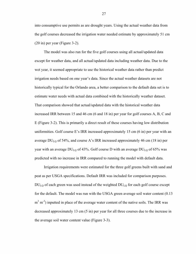
27
into consumptive use permits as are drought years. Using the actual weather data from
the golf courses decreased the irrigation water needed estimate by approximately 51 cm
(20 in) per year (Figure 3-2).
The model was also run for the five golf courses using all actual/updated data
except for weather data, and all actual/updated data including weather data. Due to the
wet year, it seemed appropriate to use the historical weather data rather than predict
irrigation needs based on one year’s data. Since the actual weather datasets are not
historically typical for the Orlando area, a better comparison to the default data set is to
estimate water needs with actual data combined with the historically weather dataset.
That comparison showed that actual/updated data with the historical weather data
increased IRR between 15 and 46 cm (6 and 18 in) per year for golf courses A, B, C and
E (Figure 3-2). This is primarily a direct result of these courses having low distribution
uniformities. Golf course E’s IRR increased approximately 15 cm (6 in) per year with an
average DULQ of 54%, and course A’s IRR increased approximately 46 cm (18 in) per
year with an average DULQ of 43%. Golf course D with an average DULQ of 65% was
predicted with no increase in IRR compared to running the model with default data.
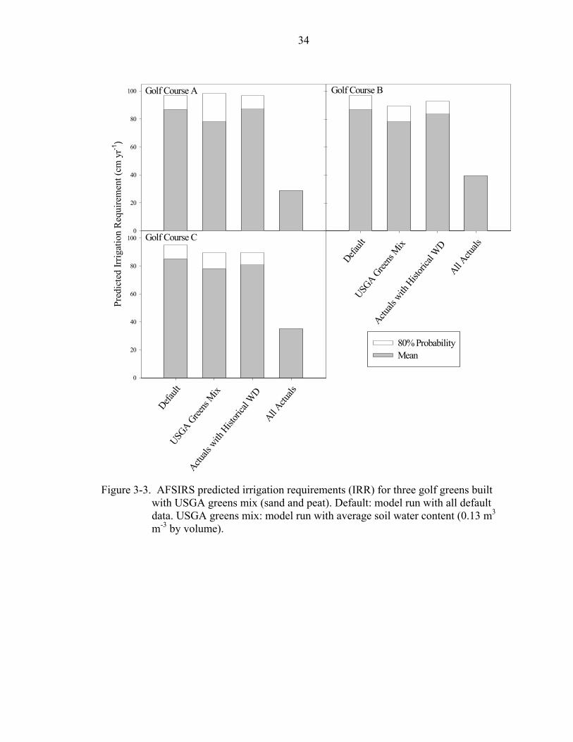
Irrigation requirements were estimated for the three golf greens built with sand and
peat as per USGA specifications. Default IRR was included for comparison purposes.
DULQ of each green was used instead of the weighted DULQ for each golf course except
for the default. The model was run with the USGA green average soil water content (0.13
m3 m-3) inputted in place of the average water content of the native soils. The IRR was
decreased approximately 13 cm (5 in) per year for all three courses due to the increase in
the average soil water content value (Figure 3-3).

28
Predictions with all actual data, including USGA greens mix average water content,
and historical weather data resulted in IRR approximately the same for all three courses
when compared to the default IRR (Figure 3-3). This is because the average DULQ on the
three greens at each course (ranged from 50% to 69%) was higher than the weighted
DULQ of each golf course, and the higher average soil water content makes up for the
DULQ being lower than the default 75%. The model was run with all actual data including
USGA greens mix average water content. Because actual weather datasets had high
rainfall amounts, IRR was decreased about 51 cm (20 in) per year for all three golf
courses.
Golf courses A, B, C, and D each had a mean predicted IRR of about 86 cm (34 in)
and golf course E had an IRR of 74 cm (29 in) (Figure 3-2). Based on rainfall and ETo,
the mean IRR was predicted to be about the same additional amount (depth) as the ETo
values (Table 3-3). The IRR on the District issued consumptive use permit (CUP) for golf
courses C, D, and E are slightly higher than the mean IRR because the permit accounts
for a two in ten year drought. According to their respective permits, golf course A
received 30% more water than the mean IRR because of a deep water table, and golf
course B received 21% more than the 80% predicted value because a 70% irrigation
efficiency value was used instead of 75%. Using the measured precipitation rates and run
times, the depth of irrigation water applied to the fairway (largest irrigated area) of the
control hole was determined. The golf courses managers irrigated from 12 to 67% less
than what the model (default values) predicted was needed. Two golf courses irrigated
approximately half of what the model (default values) predicted as the IRR. This was due
to the rainfall of above normal, which was not accounted for by the model. Accounting

29
for the actual rainfall received on each golf course, the turf managers irrigated from 42%
less than they needed to 58% more than they needed.
Conclusions
Investigations of the AFSIRS model indicate that when actual data (crop
coefficients, distribution uniformity, and rooting depth) was included in the model it
predicted similar water needs compared to the default prediction for only one of the five
golf courses evaluated. The use of actual data resulted in IRR increasing between 15 and
46 cm (6 and 18 in) per year for the golf courses. This was typically a direct result of
those courses having low distribution uniformities. When only distribution uniformities
were substituted for the default irrigation efficiency, IRR increased between 13 and 76
cm (5 and 30 in) per year. Although DULQ provides an estimate of irrigation efficiency,
the true efficiency of the system may be higher or lower than the measured DULQ.
Weather has a significant potential to influence inputs and predicted values but
since the AFSIRS is used primarily as a prediction equation, it is difficult to use current
weather patterns to predict long-term future needs. Weather datasets consisting of more
than one year of data would provide a better comparison to estimates calculated using
long-term, historical weather data.
Although a green built with USGA greens mix may require less water than the rest
of the golf course, IRR issued on consumptive use permits do not account for this
difference. But because of the stresses to a green (low mowing heights and high traffic),
these areas may need the same, or more, water than the rest of the course on a per acre
basis.
Precipitation rates and run times can provide an estimate for how much water
actually was applied to certain areas on golf courses. Because of the high rainfall

30
amounts during the year, golf course managers used less water than the predicted
irrigation requirements with default data. The high rainfall was not accounted for in the
predicted IRR using default data. When comparing water use to irrigation requirements
with updated/actual data, managers used less and more water than what was predicted.
This is a result of courses receiving different amounts of rainfall, and having different
DULQ values.

31
Table 3-1. Soil types and average water contents for the five golf courses, average water content of all soil types in the model database, and average water content of a USGA green
Golf course Soil type Average water content (m3 m-3) A Astatula sand 0.07 B Astatula sand 0.07 C Astatula sand 0.07 D Candler sand 0.06 E Blanton fine sand 0.10 Avg. of all soil types in -- 0.12 USGA green -- 0.13
Table 3-2. Mean squares for the analysis of variance on rooting depths as influenced by
golf course, location within golf course, and month Source of variation df F value † Golf course 4 0.57 ns Location (golf course) 10 1.40 ns Month 3 5.83 ** Error 42 † *, **, *** significant at the 0.05, 0.01, 0.001 levels, respectively. ns, nonsignificant at the 0.05 level Table 3-3. Mean rainfall, reference ET, estimated mean irrigation requirement, irrigation
requirement issued on consumptive use permit, mean irrigation requirement using updated/actual data, and applied irrigation
Golf Course
Rainfall
ETo
IRR†
CUP IRR‡
IRR§
Irrigation
---------------------cm--------------------- A 175 84 86 145 45 28 B 145 106 86 104 43 38 C 124 97 86 91 48 76 D 145 92 86 97 36 53 E 132 98 74 94 77 45
† irrigation requirements predicted using AFSIRS with default values ‡ CUP = District issued consumptive use permit
§ irrigation requirements predicted using updated/actual data

32
ET
Histo
rical
Actua
l
Yea
rly A
vera
ge m
m d
ay-1
3.0
3.2
3.4
3.6
3.8
4.0Rainfall
Histo
rical
Actua
l
Yea
rly A
vera
ge m
m d
ay-1
2
3
4
5
6
7
A
B
CD
A
BC
D
EE
B.A.
Figure 3-1. Yearly average reference ET (A) and rainfall (B) for the 20 year historical
weather dataset (Orlando), and for the one year of on-site weather data from each of the five golf courses. Letters denote the five courses. Horizontal dashed lines indicate the upper and lower limits of the 95% probability of occurrence for the historical data.

33
0
20
40
60
80
100
120
140
160
180 Golf Course A Golf Course B
Golf Course C
Pred
icte
d Irr
igat
ion
Req
uire
men
t (cm
yr-1
)
0
20
40
60
80
100
120
140
160
180 Golf Course D
Default
Update
d Kc
Actual
DUActu
al RD
Actual
WD
Actuals
with
Hist
orical
WD
All Actu
als
80% ProbabilityMean
Golf Course E
Default
Update
d Kc
Actual
DUActu
al RD
Actual
WD
Actuals
with
Hist
orical
WD
All Actu
als
0
20
40
60
80
100
120
140
160
180
Figure 3-2. AFSIRS predicted irrigation requirements (IRR) for five golf courses.
Default: model run with all default data. All others were run with actual values collected on-site or in the case of crop coefficients, published values.
34
Golf Course A
0
20
40
60
80
100 Golf Course B
Default
USGA G
reens
Mix
Actuals
with
Hist
orical
WD
All Actu
als
80% ProbabilityMean
Golf Course C
Default
USGA G
reens
Mix
Actuals
with
Hist
orical
WD
All Actu
als
Pred
icte
d Irr
igat
ion
Req
uire
men
t (cm
yr-1
)
0
20
40
60
80
100
Figure 3-3. AFSIRS predicted irrigation requirements (IRR) for three golf greens built
with USGA greens mix (sand and peat). Default: model run with all default data. USGA greens mix: model run with average soil water content (0.13 m3 m-3 by volume).

CHAPTER 4 SENSITIVITY ANALYSIS OF THE AGRICULTURAL FIELD SCALE IRRIGATION
REQUIREMENT SIMULATION (AFSIRS) AND THE FAO 56 PENMAN-MONTEITH EQUATION
Introduction
To provide a better understanding for how a model works and how the input
parameters influence the outputs, a sensitivity analysis can be utilized. A sensitivity
analysis requires varying selected parameters individually through an expected range of
values and then comparing the range of output values from each input variable (James
and Burges, 1982). This analysis technique determines which parameters have the
greatest impact on the output, therefore determining the level of measurement accuracy
of each input variable. The South Florida Water Management District used a sensitivity
analysis to assess the impact of parameter errors on the uncertainty in output values for
the South Florida Water Management Model and the Natural Systems Model (Loucks
and Stedinger, 1994). Once the key errors were identified, it was possible to determine
the extent to which parameter uncertainty can be reduced through field investigations,
development of better models, and other efforts (Loucks and Stedinger, 1994).
The Agricultural Field Scale Irrigation Requirement Simulation (AFSIRS) is the
model used by the St. Johns River Water Management District, South Florida Water
Management District, and North Florida Water Management District to predict irrigation
requirements (IRR) for golf courses. It is a numerical simulation model which estimates
IRR for Florida crops, soil, irrigation systems, climate conditions, and irrigation
management practices (Smajstrla, 1990). The FAO 56 Penman-Monteith equation (Allen
35

36
et al., 1998) was found to be the most consistent model for determining reference
evapotranspiration (ETo) for Florida conditions (Jacobs and Satti, 2001). This equation
can be used to calculate ETo in a computer program such as REF-ET (a stand-alone
computer program that calculates reference ET from meteorological data made available
by the user (Allen, 2002)). These calculated reference ET rates can be used to create site-
specific datasets for use with the AFSIRS model.
To establish how the output from the AFSIRS model and the FAO 56 Penman-
Monteith equation (Allen et al., 1998) respond to changes in their inputs, a study was
conducted using sensitivity analysis. The objective of this research was to determine what
parameters have the greatest impact on the irrigation requirement predicted with the
AFSIRS model and reference evapotranspiration (ETo) using the FAO 56 Penman-
Monteith equation (Allen et al., 1998).
Materials and Methods
Agricultural Field Scale Irrigation Requirement Simulation (AFSIRS)
Crop Coefficient (Kc), distribution uniformity (DULQ) (in place of irrigation
application efficiency), average and maximum rooting depth, and average soil water
content were the parameters that were analyzed for sensitivity on the AFSIRS model.
Individual model runs were made using a range of values for each parameter. The values
were changed in increments from the starting point, in both directions, depending on the
size of the range. Each of the four input parameters were analyzed separately, while the
other parameter values remained constant. The constant value for the parameters not
being analyzed was the average value observed for each parameter from a concurrent golf
course water use study where site-specific data was collected from five golf courses for
predicting IRR using the AFSIRS model (Pressler, 2003).

37
Starting values and ranges were chosen for the four parameters based on the data
collected in the concurrent water use study. The starting value for each parameter was the
average value calculated for each parameter. The Kc value starting point for this study
was 0.7. This value was changed in increments of 0.1 in both directions, and ranged from
0.5 to 1.0. The DULQ starting point value was 50%. The values were changed in
increments of 10% in both directions, and ranged from 20% to 100%. Rooting depths had
two starting points. The average depth starting point was 12.7 cm and maximum depth
starting point was 50.8 cm (5 and 20 in, respectively). These depths were changed in
increments of 2.54 and 10.2 cm (1 and 4 in) in both directions, and ranged from 2.54 and
10.2 to 20.3 and 81.3 cm (1 and 4 to 8 and 32 in), respectively. Average soil water
content starting point was 0.09 m3 m-3, was changed in increments of 0.02 m3 m-3 in both
directions, and ranged from 0.03 to 0.17 m3 m-3 (by volume).
FAO 56 Penman-Monteith Equation
Maximum and minimum temperature, maximum and minimum relative humidity,
mean solar radiation, mean soil heat flux, and mean wind speed were parameters that
were analyzed for sensitivity on the FAO 56 Penman-Monteith equation (Allen et al.,
1998) in the REF-ET program. Each of the eight input parameters were analyzed
separately, while the other parameter values remained constant. The starting values for
each parameter were the average values observed from collected weather data during the
concurrent water use study. The values were changed in increments from the starting
point, in both directions, depending on the size of the range.
Because the temperature data collected by the weather station and analyzed in REF-
ET was in Fahrenheit, the values used and reported in the sensitivity analysis are also in
Fahrenheit. The min. temperature starting point was 60oF. The values were changed in

38
increments of 10oF in both directions, and ranged from 20 to 80oF. The max. temperature
starting point value was 80oF. The values were changed in increments of 10oF in both
directions, and ranged from 40 to 100oF. The min. relative humidity starting point was
50%. The values were changed in increments of 10% in both directions, and ranged from
10 to 90%. The max. relative humidity starting point was 95%. The values were changed
in increments of 10% in both directions, and ranged from 60 to 100%. The mean solar
radiation starting point value was 160 W/m2. The values were changed in increments of
40 W/m2 in both directions, and ranged from 0 to 320 W/m2. The mean soil heat flux
starting point was 0 W/m2. The values were changed in increments of 5 W/m2 in both
directions, and ranged from -25 to 15 W/m2. The mean wind speed starting point value
was 8 km/hr. The values were changed in increments of 1.61 km/hr in the decreasing
direction and 4.8 km/hr in the increasing direction, and ranged from 3.2 to 37 km/hr.
Results and Discussion
Agricultural Field Scale Irrigation Requirement (AFSIRS) Sensitivity Analysis
Changes in DULQ resulted in the largest changes in IRR (Figure 4-1). Changing a
DULQ from 40% to 80%, a 100% increase, resulted in a 65% decrease in irrigation
requirement. The Irrigation Association suggests that a 70% DULQ is expected and an
80% DULQ is achievable for a golf course. Modifying Kc values had the second largest
impact on IRR. IRR increased linearly as Kc values decreased. A 15% increase or
decrease of the starting point resulted in a 20% change in IRR in the respective direction.
Changes in rooting depth and average soil water content had very little impact on
IRR. As rooting depth and average soil water content increase, IRR decreases. Increasing
and decreasing both inputs by 60% of the starting points resulted in less than 16%
increases and decreases in IRR.

39
FAO 56 Penman-Monteith Equation Sensitivity Analysis
A change in max. temperature resulted in the largest change in ETo (Figure 4-2).
A 25% increase of the starting point resulted in a 45% increase in ETo. Modifying mean
solar radiation had the second greatest impact on ETo. A 50% increase of the starting
point resulted in a 33% change in ETo.
Changes in min. relative humidity and mean wind speed had the third and fourth
largest impact on ETo, respectively. Increasing both inputs by 60% of the starting points
resulted in a 25% decrease in ETo for min. relative humidity, and a 15% increase in ETo
for mean wind speed. Changes in min. temperature, mean soil heat flux, and max. relative
humidity had very little impact on ETo. A 25% decrease of the starting points for each of
the three parameters resulted in a less than 8% increase in ETo.
Conclusions
Sensitivity analysis further indicated that there can be significant differences
between default values and true values when using the AFSIRS model. This was most
apparent with DULQ (in place of efficiency) and crop coefficients. Because these
parameters have the most impact on IRR, the data used in these inputs needs to have the
highest accuracy. By collecting site-specific data, a true picture can be illustrated for
irrigation requirements, and as a result, more water may be conserved. According to the
AFSIRS, by attaining a relatively high DULQ (60 to 80%), golf course managers can
greatly reduce wasteful water use, and as a result, meet or stay within their water
allotments.
Because it is difficult to determine site-specific crop coefficients in the field,
published data is the best alternative. More research needs to be conducted to determine
Kc values for different types of turfgrasses grown under Florida conditions.
40
When determining reference ET rates using REF-ET and the FAO 56 Penman-
Monteith equation (Allen et al.,1998), daily maximum temperature and mean solar
radiation have the greatest effect on the output, followed by minimum relative humidity
and mean wind speed. The data collected for these parameters with the most influence on
ETo, should be measured with the highest accuracy to reduce variability.
If the reference ET rates calculated by the FAO 56 Penman-Monteith equation
(Allen et al., 1998) are used in the AFSIRS model, DULQ and Kc values as well as daily
maximum temperature and mean solar radiation have a great impact on predicted
irrigation requirement. But because three of those parameters are out of a golf course
manager’s control, the focus should be on improving DULQ to conserve water.

41
-7 5
-5 0
-2 5
0
2 5
5 0
7 5
1 0 0
1 2 5
1 5 0
1 7 5K c D U L Q
% C han ge in In itia l P aram eter In p u t
-100 -80 -60 -40 -20 0 20 40 60 80 100 120
% C
hang
e in
Irrig
atio
n R
equi
rem
ent
-7 5
-5 0
-2 5
0
2 5
5 0
7 5
1 0 0
1 2 5
1 5 0
1 7 5 R oo tin g D ep th S o il (A W C )
Figure 4-1. Sensitivity analysis of the AFSIRS model output. Values across x-axis
represent a typical value as the starting point (0) and a range of values in the % change of the initial value.

42
-40
-20
0
20
40
60
80
Max. Temp.Mean Solar Rad.
Mean Wind SpeedMin. Rel. Humidity
% Change in Climatic Parameter
-100 -50 0 50 100 150
% C
hang
e in
Ref
eren
ce E
vapo
trans
pira
tion
Rat
e
-40
-20
0
20
40
60
80Min. Temp.Mean Heat Flux
-100 -50 0 50 100 150 200
Max. Rel. Humidity
Figure 4-2. Sensitivity analysis of the FAO 56 Penman-Monteith equation (Allen et al.,
1998). Values were changed across a range of typical values. Values across x-axis represent a typical value as the starting point (0) and a range of values in the % change of the initial value.

CHAPTER 5 SUMMARY AND CONCLUSIONS
Using site-specific data instead of default values in the AFSIRS model can result in
site-specific estimates of irrigation requirements on golf courses. For prediction purposes
it is better to use long-term (historical) weather data rather than short-term data.
It is important for golf course managers to be familiar with how their Water
Management District determines golf course irrigation requirements. Knowing what data
goes into the AFSIRS model, can allow a manager to use their allotted water more
effectively, e.g. improving distribution uniformity. Evaluation of the AFSIRS model and
its effectiveness in predicting irrigation requirements using default and actual (on-site)
data from five golf courses was discussed in Chapter 3. The following results were
obtained:
• Updated crop coefficients resulted in IRR predictions to drop approximately 25.4 cm (10 in) from the default estimates. Actual rooting depths caused IRR predictions to increase approximately 17.8 cm (7 in).
• Replacing distribution uniformities with the default irrigation efficiency, caused the greatest change in IRR predictions (increase between 12.7 to 76.2 cm or 5 to 30 in depending on the golf course).
• The one year of weather data collected at each golf course represented 56 and 109 cm (22 and 43 in) more than the average rainfall compared to the 20 year historical weather dataset. As a result, the estimates using the actual weather data decreased IRR predictions by approximately 51 cm (20 in).
• Due to the wet year, the model was run with all actual data and with the historical weather dataset. This combination of actual and historical data resulted in an increase in IRR predictions of 15 to 46 cm (0 to 18 in).
43

44
• Predictions with all actual data, including USGA green soil substrate average water content, and historical weather data resulted in little to no change in IRR for the three courses with USGA specification greens.
Sensitivity analysis allowed for a better understanding of how the AFSIRS model
and FAO 56 Penman-Monteith equation (Allen et al., 1998) work. It indicated what
inputs had the greatest impact on the outputs. The inputs with the most influence on
outputs of interest needs to be measured with the highest accuracy to reduce variability.
Sensitivity analysis on the AFSIRS model and FAO 56 Penman-Monteith equation
(Allen et al., 1998) was discussed in Chapter 4. The following results were obtained:
• Sensitivity analysis on the AFSIRS model further indicated that distribution uniformity (irrigation efficiency input) had the greatest influence on the IRR prediction value, followed by: Kc, rooting depth, and average soil water content. Changing a DULQ from 40% to 80%, a 100% increase, resulted in a 65% decrease in irrigation requirement.
• Sensitivity analysis on the FAO 56 Penman-Monteith (Allen et al., 1998) using the REF-ET program to predict ETo illustrated that changes in daily max. temperature resulted in the largest changes in ETo, followed by: mean solar radiation, min. relative humidity, mean wind speed, min. temperature, max. relative humidity, and mean soil heat flux. A 25% increase of the starting point for max. temperature resulted in a 45% increase in ETo, and a 50% increase of the starting point for mean solar radiation resulted in a 33% change in ETo.

APPENDIX SAS PROGRAMS
Program to organize weather station data into columns for REF-ET. data ds1; infile 'd:\glm test 91803.prn' firstobs=2; input year day min Temp RHb solar soil soil2 windsp @@; /*drop bar;*/ drop min; soilmean=(soil+soil2)/2; drop soil soil2; /*proc print; run;*/ cards; proc sort; by year day; proc means noprint; by year day; var temp RHb; output out=data1 min=mn_t mn_RH max=mx_t mx_RH; proc means data=ds1 noprint; by year day; var solar soilmean windsp; output out=data2 mean=m_sol m_soil m_wind ; proc sort data=data1; by year day; proc sort data=data2; by year day; data all; merge data1 data2; by year day; /*proc print;*/ proc print data=all; var year day mn_t mx_t mn_RH mx_RH m_sol m_soil m_wind; run;
45

46
Rooting depths influenced by month, golf course, and location within golf course using analysis of variance procedure. Title 'Mean Rooting Depth'; Data; Input GC $ trt $ loc $month $ RD; Cards; proc sort; by trt; proc glm;by trt; class loc gc month; model RD= gc loc(gc) month; test h=gc e=loc(gc); means loc(gc)/lsd lines; means month/lsd lines; run;

REFERENCES
A forum on sensitivity analysis. 2004. Institute for Systems, Informatics, and Safety. Joint Research Centre. The European Commission. [Online]. Available at http://sensitivity-analysis.jrc.cec.eu.int (Verified 16 June 2004).
Allen, R.A. 2002. REF-ET reference evapotranspiration software. [Online] http://www.kimberly.uidaho.edu/REF-ET/ (Verified 3 Feb. 2004).
Allen, R.G., L.S. Pereira, D. Raes and M. Smith. 1998. Crop evapotranspiration – guidelines for computing crop water requirements. FAO Irrig. and Drain. Paper56.
American Society of Agricultural Engineers (ASAE). 2001. Test procedure for determining the uniformity of water distribution of center pivot and lateral move irrigation machines equipped with spray or sprinkler nozzles. Irrig. Assoc. and the ASAE Sprinkler Irrigation Comm. ANSI/ASAE Standard S436.1. ASAE St.Joseph, MI.
Beard, J.B. 1973. Turfgrass science and culture. Prentice-Hall. Englewood Cliffs, NJ.
Beard, J.B. 1982. Turfgrass management for golf courses. Macmillan Publishing Company. New York, NY.
Beard, J.B. 1985. An assessment of water use by turfgrasses. In V.A. Gibeault and S.T. Cockerham (ed.) Turfgrass water conservation. Cooper. Ext Publ. 21405, Univ. of California, Oakland, CA.
Beard, J.B. 2002. Turfgrass management for golf courses 2nd ed. Ann Arbor Press. Chelsea MI.
Beard, J.B., R.L. Green, and S.I. Sifers. 1992. Evapotranspiration and leaf extension rates of 24 well-watered, turf-type Cynodon genotypes. HortScience 27:986-988.
Bowman, D.C., L.B. McCarty, and J. Camberato. 2001. Water management in turf. p. 261-280. In L.B McCarty (ed.) Best golf course management practices. Prentice- Hall, Inc. Upper Saddle River, NJ.
Brady, N.C., and R.R. Weil. 1999. Elements of the nature and properties of soils 12th ed. Prentice-Hall, Inc. Upper Saddle River, NJ.
47

48
Brown, P.W., and D.M. Kopec. 2000. Converting reference evapotranspiration into turf water use. Turf irrigation management series: II. Publ. AZ1195. Available online at http://ag.arizona.edu/pubs/water/az1195.pdf (Verified 4 February 2004).
Brown, P.W., D.M. Kopec, and C.F. Mancino. 1988. Estimating turfgrass water use with AZMET. Turfgrass & Ornamentals Research Summary. Arizona Agric. Exp. Stn. P-75:25-33.
Brown, P.W., C. F. Mancino. M.I. Young, T. L. Thompson, P.J. Wierenga, and D.M. Kopec. 2001. Penman monteith crop coefficients for use with desert turf systems. Crop Sci. 41:1197-1206.
Carrow, R. N. 1995. Drought resistant aspects of turfgrasses in the southeast: evapotranspiration and crop coefficients. Crop Sci. 35:1685-1690.
Florida Automated Weather Network (FAWN). 2004. [Online]. Available at http://fawn.ifas.ufl.edu (Verified 16 June 2004).
Goss., R.L., and A.G. Law. 1967. Performance of bluegrass varieties at two cutting heights and two nitrogen levels. Agron. J. 59:516-518.
Haydu, J.J., and A.W. Hodges. 2002. Economic impacts of the Florida golf industry [Online]. Available at http://economicimpact.ifas.ufl.edu/publications/EIR02-4r.pdf. (Verified 16 June 2004). University of Florida Economic Information Report.
Higgins, J., and L.B. McCarty. 2001. Golf course construction and renovation. p. 119-148. In L.B. McCarty (ed.) Best golf course management practices. Upper Saddle River, NJ.
Huck, M. 1997. Irrigation design, rocket science, and the space program. USGA Green Section Record. 35(1):1-7.
Hummel, N.W., Jr. 1993. Rationale for the revisions of the USGA green construction specifications. USGA Green Section Record. 31(2):7-21.
Irrigation Association (IA). 2003. Certified golf irrigation auditor training manual. Irrigation Assoc. America. Falls Church, VA.
Jacobs, J., and S. Satti. 2001. Evaluation of reference evapotranspiration methodologies and AFSIRS crop water use simulation model. Publ. SJ2001-SP8. Available online at http://www.sjrwmd.com/programs/outreach/pubs/techpubs/sj2001-sp8.pdf (Verified 16 June 2004).
James, L. D., and S.J. Burges. 1982. Selection, calibration, and testing of hydrologic models. p. 437-470. In Hydrologic modeling of small watersheds. Amer. Soc. Agric. Eng., St. Joseph, MI.

49
Kim, K.S., and J.B. Beard. 1983. Comparitive ET rates of eleven major warm-season turfgrasses grown under both uniform and optimal cultural regimes. p. 127. In Agronomy abstracts. ASA, Madison, WI.
Kneebone, W.R., and I.L. Pepper. 1982. Consumptive water use by sub-irrigated turfgrasses under desert conditions. Agron. J. 74:419-423.
Loucks D.P., and J.R. Stedinger. 1994. Sensitivity and uncertainty analysis in hydrologic simulation modeling of the South Florida Water Management District. School of Civil and Environmental Engineering, Cornell Univ. Ithica, NY.
McCarty, L.B., G. Landry, Jr., and A.R. Mazur. 2001.Turfgrass. p. 3-44. In L.B.McCarty (ed.) Best Golf Course Management Practices. Upper Saddle River, NJ.
Meyer, J.L., and B.C. Camenga. 1985. Irrigation systems for water conservation. p. 105-112. In V.A. Gibeault and S.T. Cockerham (ed.) Turfgrass water conservation. Cooper. Ext. Publ. 21405, Univ. of California, Oakland, CA.
Miller, G.L., N.D. Pressler, and M. Dukes. 2003. How uniform is coverage of your irrigation system? Golf Course Manage. 71(8):100-102.
National Golf Foundation. 2004. Frequently asked questions about the game andbusiness of golf in the United States [Online]. Available at http://www.ngf.org/cgi/who faq.asp#2 (Verified 16 June 2004).
Olexa, M.T., L. Minton, D. Miller, and S. Corbett. 1998. Handbook of Florida water regulation: water management districts. FL Extension Bull. 039, FL Coop. Ext. Serv., Gainesville, FL.
Par, T.W., R. Cox, and R.A. Plant. 1984. The effects of cutting height on root distribution and water use of ryegrass turf. J. Sports Turf Res. Inst. 60:45-53.
Pira, E.S. 1997. A guide to golf course irrigation system design and drainage. Ann Arbor Press, Inc. Chelsea, MI.
Pitts, D., K. Peterson, and R. Fastenau.1996. Field assessment of irrigation system performance. Appl. Eng. Agric. 12:307-313.
Pressler, N. 2003. Evaluation of golf course irrigation system performance and the effects of irrigation amounts on turf quality and rooting depths of golf course turfgrasses. M.S. thesis. Univ. of Florida, Gainesville.
St. Johns River Water Management District (SJRWMD). 2002. Applicants handbook: consumptive uses of water, chapter 40C-2, F.A.C. [Online]. Available at http://www.sjrwmd.org/programs/regulation/index.html (Verified 16 June 2004).
50
St. Johns River Water Management District (SJRWMD). 2004. Water resource permitting program overview: consumptive use permitting. [Online]. Available at http://sjr.state.fl.us/programs/regulation/cup/overview.html (Verified 16 June2004).
SAS Institute. 1999. SAS user’s guide: Statistics. 8th ed. SAS Institute, Inc. Cary, NC.
Smajstrla, A.G., 1990. Technical Manual: Agricultural field scale irrigation requirements simulation (AFSIRS) model, Version 5.5, Agricultural Engineering Department, Univ. Florida, FL.
Smajstrla, A.G , and F.S. Zazueta. 1998. Estimating crop irrigation requirements for irrigation system design and consumptive use permitting. Publ. AE254. Univ. of Florida. Gainesville, FL.
Snyder, R.L. 1986. Evapotranspiration-based irrigation scheduling-the CIMIS experience. p.245-263. In Irrig. Assoc. Tech. Conf. Proc. San Antonio, TX.
Soil Conservation Service (SCS). 1970. Irrigation water requirements. Technical Release No. 21. USDA Soil Conservation Service. Washington, D.C.
Thompson, K. 2002. What’s uniformity worth? Improving distribution uniformity cansave golf courses money [Online]. Available at http://irrigation.org/ibt/ibt1002/p38.htm (Verified 16 June 2004).
Unruh, J.B., J.L. Cisar, and G.L. Miller. 1999. Mowing. p.103-108. In J.B Unruh and M.L. Elliot (eds.) Best management practices for Florida golf courses, 2nd ed. Institute of Food and Agricultural Sciences, Univ. Florida, FL.
Wilson, T.P., and D.F. Zoldoske. 1997. Evaluating sprinkler irrigation uniformity [Online]. Available at http://www.wateright.org/site/publications/970703.html (Verified 16 June 2004).

BIOGRAPHICAL SKETCH
Mark Mitchell was born in Palm Beach Gardens, Florida, June 4, 1980. Mark
graduated in 2002 with a Bachelor of Science in Turfgrass Science. Mark enrolled in the
horticultural science graduate program in the Fall of 2002. After graduation in 2004, he
plans to work as an assistant superintendent in Jacksonville, FL.
51
Related Documents