Evaluation of pollutant loads from stormwater BMPs to receiving water using load frequency curves with uncertainty analysis

ww.sciencedirect.com

wat e r r e s e a r c h 4 6 ( 2 0 1 2 ) 6 8 8 1e6 8 9 0

Available online at w

journal homepage: www.elsevier .com/locate/watres

Evaluation of pollutant loads from stormwater BMPsto receiving water using load frequency curveswith uncertainty analysis

Daeryong Park a,*, Larry A. Roesner b

a Illinois State Water Survey, Prairie Research Institute, University of Illinois at Urbana-Champaign, 2204 Griffith Dr., Champaign, IL

61820-7463, USAbDepartment of Civil and Environmental Engineering, Colorado State University, Fort Collins, CO 80523-1372, USA

a r t i c l e i n f o

Article history:

Received 26 August 2011

Received in revised form

12 April 2012

Accepted 15 April 2012

Available online 22 April 2012

Keywords:

Stormwater

Best management practices

k-C* model

First-order second-moment

Storage, treatment, overflow and

runoff model (STORM)

Load frequency curve

Total daily maximum load

* Corresponding author. Tel.: þ1 970 988 030E-mail addresses: [email protected] (D.

0043-1354/$ e see front matter ª 2012 Elsevdoi:10.1016/j.watres.2012.04.023

a b s t r a c t

This study examined pollutant loads released to receiving water from a typical urban

watershed in the Los Angeles (LA) Basin of California by applying a best management

practice (BMP) performance model that includes uncertainty. This BMP performance model

uses the k-C* model and incorporates uncertainty analysis and the first-order second-

moment (FOSM) method to assess the effectiveness of BMPs for removing stormwater

pollutants. Uncertainties were considered for the influent event mean concentration (EMC)

and the aerial removal rate constant of the k-C* model. The storage treatment overflow and

runoff model (STORM) was used to simulate the flow volume from watershed, the bypass

flow volume and the flow volume that passes through the BMP. Detention basins and total

suspended solids (TSS) were chosen as representatives of stormwater BMP and pollutant,

respectively. This paper applies load frequency curves (LFCs), which replace the exceed-

ance percentage with an exceedance frequency as an alternative to load duration curves

(LDCs), to evaluate the effectiveness of BMPs. An evaluation method based on uncertainty

analysis is suggested because it applies a water quality standard exceedance based on

frequency and magnitude. As a result, the incorporation of uncertainty in the estimates of

pollutant loads can assist stormwater managers in determining the degree of total daily

maximum load (TMDL) compliance that could be expected from a given BMP in

a watershed.

ª 2012 Elsevier Ltd. All rights reserved.

1. Introduction reliably simulating pollutant removal. Input flows and

Urban stormwater runoff contains significant concentrations

of a variety of pollutants and is a principal cause of the dete-

rioration of receiving water quality in urban areas. Structural

best management practices (BMPs) are widely applied to

reduce nonpoint source pollution and attenuate peak runoff.

However, the many uncertainties associated with BMP

performance preclude models of BMP performance from

4.Park), Larry.Roesner@colier Ltd. All rights reserved

pollutant concentrations vary from storm to storm andwithin

individual storms, and BMP pollutant removal mechanisms

are not sufficiently accurate. Therefore, the computed (esti-

mated) pollutant loads and concentrations emanating from

a BMP model are uncertain. As regulatory agencies move

toward BMP effluent criteria or total daily maximum load

(TMDL) allocations for receiving waters, it becomes increas-

ingly important to understand the certainty with which we

ostate.edu (L.A. Roesner)..

wat e r r e s e a r c h 4 6 ( 2 0 1 2 ) 6 8 8 1e6 8 9 06882

can estimate the performance of a BMP or, conversely, to

understand uncertainty associated with an estimated effluent

concentration from a BMP.

To evaluate the TMDL, load duration curves (LDCs) have

been developed by Stiles (2001). Several researchers (Stiles,

2001; Cleland, 2002, 2003; Bonta and Cleland, 2003; and

O’Donnell et al., 2005) have utilized LDCs to estimate the

TMDL because this method is capable of identifying daily

loads that account for the variable nature of water quality

with time. A maximum concentration standard and a hydro-

logic flow duration curve (FDC) can identify a TMDL that is

appropriate for the full range of streamflow conditions, and

the maximum daily load can be verified for any given day (US

EPA, 2007). Although LDCs have becomemorewidely used and

accepted for TMDL estimation, it is necessary to take the

pollutant-reducing physical model into consideration. The

current LDCmethod only accounts for flow variables and does

not consider other variables because it does not incorporate

certain physical models (Shen and Zhao, 2010).

The purpose of this paper is to present an approach for

estimating the pollutant load exceedance frequencies result-

ing from BMPs with estimates of the certainties (or uncer-

tainties) of those estimates. If a TMDL is specified as an

average load and an upper limit on that loadwhich is not to be

exceededmore than n times per year, the algorithm presented

will assist in the design of a BMP that will meet the criteria

with 95% certainty. The method is simple, but it is a step

forward in linking BMP performance to receiving water

quality. The conceptual model used is the storage, treatment,

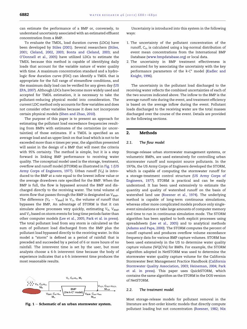
overflow and runoff model (STORM) as illustrated in Fig. 1 (US

Army Corps of Engineers, 1977). Urban runoff (VR) is intro-

duced to the BMP at a rate equal to the lowest inflow value or

the average drawdown rate specified for the BMP. When the

BMP is full, the flow is bypassed around the BMP and dis-

charged directly to the receiving water. The total volume of

storm flow that passes through the BMP is designated as VBMP.

The difference (VR � VBMP) is VO, the volume of runoff that

bypasses the BMP, An advantage of STORM is that it can

simulate above processes very quickly, estimating VR, VBMP

andVO based on stormevents for long time periods faster than

other computer models (Lee et al., 2005; Park et al. in press).

The total pollutant load from any storm is calculated as the

sum of pollutant load discharged from the BMP plus the

pollutant load bypassed directly to the receiving water. In this

model a “storm” is defined as a period of rainfall that is

preceded and succeeded by a period of 6 or more hours of no

rainfall. The interevent time is set by the user, but most

analysts choose a 6-h interevent time because the body of

experience indicates that a 6-h interevent time produces the

most reasonable results.

Fig. 1 e Schematic of an urban stormwater system.

Uncertainty is introduced into this system in the following

ways:

1. The uncertainty of the pollutant concentration of the

runoff, Cin is calculated using a log-normal distribution of

event mean concentrations from the International BMP

Database (www.bmpdatabase.org) or local data.

2. The uncertainty in BMP treatment effectiveness is

accounted for by associating the uncertainty with the key

performance parameters of the k-C* model (Kadlec and

Knight, 1996).

The uncertainty in the pollutant load discharged to the

receiving water reflects the combined uncertainties of each of

the two sources indicated above. The inflow to the BMP is the

average runoff rate during the event, and treatment efficiency

is based on the average inflow during the event. Pollutant

loads discharged to the receiving water are the total masses

discharged over the course of the event. Details are provided

in the following sections.

2. Methods

2.1. The flow model

Storage-release urban stormwater management systems, or

volumetric BMPs, are used extensively for controlling urban

stormwater runoff and nonpoint source pollutants. In the

1970s, the US Army Corps of Engineers developed the STORM,

which is capable of computing the stormwater runoff for

a storage-treatment control structure (US Army Corps of

Engineers, 1977). STORM is practical and can be easily

understood. It has been used extensively to estimate the

quantity and quality of watershed runoff on the basis of

watershed land use (Roesner et al., 1974). The underlying

method is capable of long-term continuous simulations,

whereas other more complicated models produce only single-

event simulations or take large amounts of computer memory

and time to run in continuous simulation mode. The STORM

algorithm has been applied to both explicit processes using

spreadsheets (Lee et al., 2005) and to analytical methods

(Adams and Papa, 2000). The STORM computes the percent of

runoff captured and produces overflow volume exceedance

frequency data for various BMP capture volumes. STORM has

been used extensively in the US to determine water quality

capture volume (WQCVs) for BMPs. For example, the STORM

algorithm adopted in NetSTORM was used to determine the

stormwater water quality capture volume for the California

Stormwater Best Management Practice Handbook (California

Stormwater Quality Association, 2003; Heineman, 2004; Park

et al. in press). This paper uses QuickSTORM, which

contains the same algorithm as the STORM in the DOS version

of NetSTORM.

2.2. The treatment model

Most storage-release models for pollutant removal in the

literature are first-order kinetic models that directly compute

pollutant loading but not concentration (Roesner, 1982; Nix

wat e r r e s e a r c h 4 6 ( 2 0 1 2 ) 6 8 8 1e6 8 9 0 6883

and Heaney, 1988; Patry and Kennedy, 1989; Segarra-Garcia

and Loganathan, 1992; Segarra-Garcia and Basha-Rivera,

1996; Lee et al., 2005). These studies applied a first-order

kinetic equation to express BMP performances and repre-

sented the results with percentages of pollutant removal as

functions of BMP storage volumes and release rates. However,

the hydraulic loading rate (HLR) is strongly correlated to

pollutant removal and is a function of both the inflow rate and

BMP surface area (Kadlec, 2000). The background concentra-

tion (C*) of outflow from the BMP can be considered constant

from storm to storm, as has been verified bymany researchers

(e.g. Schueler, 1996; Wong and Geiger, 1997; Minton, 2005).

This paper also uses the k-C* model to characterize BMP

performance. The k-C* model is defined by the following

equation (Kadlec and Knight, 1996):

Cout ¼ C� þ ðCin � C�Þe�k=q (1)

where

Cout ¼ effluent EMC (mg/L),

Cin ¼ influent EMC (mg/L),

C* ¼ background EMC or “irreducible minimum concentra-

tion” (mg/L),

k ¼ aerial removal rate constant (m/day), and

q ¼ BMP hydraulic loading rate, defined as the ratio of the

average inflow rate Q to the surface area A of the BMP, i.e., (Q/

A) (m/day).

The k-C* model has been used to model wetland perfor-

mance, and many references have verified that this model

characterizes the removal of pollutants by wetlands very well

(Kadlec and Knight, 1996; Kadlec, 2000, 2003; Braskerud, 2002;

Rousseau et al., 2004; Lin et al., 2005). Recently, the k-C* model

was used by Wong et al. (2002, 2006) and Huber (2006) to

simulate stormwater BMPs because the characteristics of

wetlands, detention basins and retention ponds are similar.

However, it is difficult to obtain a reliable prediction of

pollutant removal with the k-C* model because the determi-

nation of the parameters C* and k includes large intersystem

variabilities (Kadlec, 2000) and additional parameters, such as

temperature (Kadlec and Reddy, 2001), Damkohler number

(Carleton, 2002), flow velocity and residence time (Carleton

and Montas, 2007). Therefore, it is necessary to develop

a more simplified and generalized model for predicting

pollutant removal. Park et al. (2011) applied uncertainty

analysis to the k-C* model and successfully presented Cout as

a probability density function in detention basins depending

on Cin and q. k was represented as a function of q (Schierup

et al., 1990; Lin et al., 2005). This paper adopts this method

to simulate BMP performance.

2.3. Incorporation of uncertainty into the model

Uncertainty analysis has been used to quantify reliabilities or

probabilistic risks for a variety of engineering problems. The

first-order second-moment (FOSM)method, also known as the

first-order error (FOE) or first-order variance estimation (FOVE)

method, is one of the most general and simple methods of

uncertainty analysis. It is a first-order approximation method

because it considers only the first order of the Taylor series.

The FOSMmethod has been applied to various hydro-systems,

including storm drainage (Yen and Tang, 1976) and levee

systems (Tung and Mays, 1981). In environmental engi-

neering, several researchers have applied the FOSMmethod to

the StreeterePhelps equation, which is used to estimate dis-

solved oxygen in streamflows (Burges and Lettenmaier, 1975;

Tung and Hathhorn, 1988; Song and Brown, 1990; Melching

and Anmangandla, 1992).

The FOSMmethod has been used to estimate themargin of

safety (MOS) with respect to the TMDL (Zhang and Yu, 2004;

Franceschini and Tsai, 2008). Shirmohammadi et al. (2006)

integrated several uncertainty analysis methods, including

the Monte Carlo simulation (MCS), FOE analysis, Latin hyper-

cube sampling (LHS), and generalized likelihood uncertainty

estimation (GLUE), into the soil and water assessment tool

(SWAT) to represent the cumulative density function (CDF) of

monthly sediment reduction as a measure of BMP effective-

ness. They suggested using uncertainty analysis to improve

estimates of the MOS and TMDL. Arabi et al. (2007) charac-

terized BMP effectiveness in terms of estimated monthly

sediment reduction, total phosphorus (TP), and total nitrogen

(TN) with two types of uncertainty analysis methods: one-

factor-at-a-time (OAT) sensitivity analysis and GLUE using

SWAT. In addition, they suggested using a probabilistic esti-

mation of the MOS for TMDL development.

In urban stormwater modeling, Kleidorfer et al. (2009) and

Dotto et al. (2011) applied uncertainty analysis to the rainfall/

runoff process by the model for urban stormwater improve-

ment conceptualization (MUSIC) and the KAREN model and

build-up/wash-off processes using simple regression and

build-up/wash-off equations, respectively. The Bayesian

Monte Carlo Markov Chain (BMCMC) method was applied for

uncertainty analysis. Kleidorfer et al. (2009) focused on

measurement errors for uncertainty analysis but Dottos et al.

(2011) considered the predictive uncertainty resulting from

parameter uncertainty in the MUSIC, KAREN and build-up/

wash-off models. These studies focused on uncertainties in

runoff and pollutants from a watershed. Therefore, it was

necessary to study the uncertainty of water quality BMP

performance for the next step. Asmentioned above, Park et al.

(2011) studied the BMP performance incorporating uncer-

tainty analysis and compared the results with observed data.

This study focused on the predictive uncertainty due to

parameter uncertainties (Cin and k) in the BMP performance

model (the k-C* model) and did not consider other sources of

uncertainty. The results showed that the FOSM method is

exceptionally easy to apply to uncertainty analysis of BMP

performance compared with the derived distribution method

(DDM) and LHS because it requires only the mean and vari-

ance of the data if the probability density function is similar to

a two-parameter distribution and that its accuracy is only

slightly different (approximately 5 mg/L for confidence limits

[CLs]) from that of the LHS method. The applicability of the

FOSMmethod increases if the variable distribution is a known

two-parameter distribution.

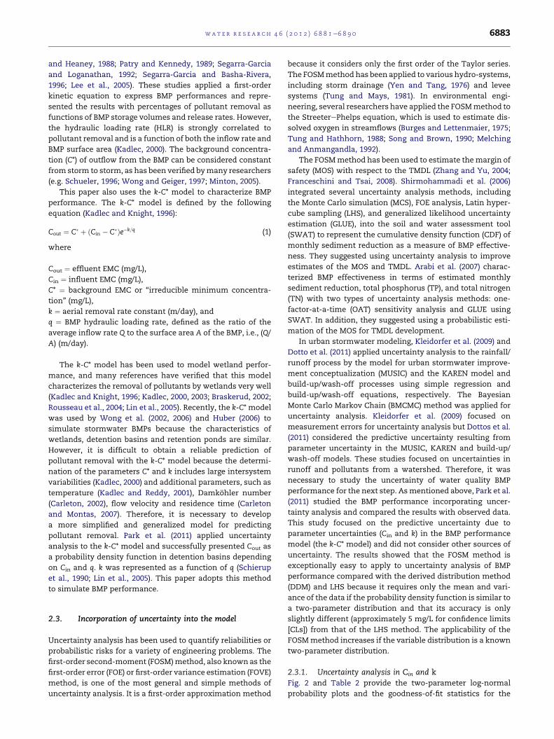
2.3.1. Uncertainty analysis in Cin and kFig. 2 and Table 2 provide the two-parameter log-normal

probability plots and the goodness-of-fit statistics for the

Fig. 2 e Log-normal probability plots of observed Cin and

Cout in detention basins.

Table 2 e Results of goodness-of-fit tests; observed Cin

and Cout from Table 1.

Test Critical value (a ¼ 0.10) Decision

Cin Cout

Chi-Square 0.663 0.860 Accept

KolmogoroveSmirnov 0.789 0.852 Accept

AndersoneDarling 0.567 0.685 Accept

wat e r r e s e a r c h 4 6 ( 2 0 1 2 ) 6 8 8 1e6 8 9 06884

observed Cin and Cout of TSS in detention basins for the BMP

sites listed in Table 1. Fig. 2 shows that the TSS distributions

for both Cin and Cout are well represented as log-normal

probability plots. Table 2 shows the results of three

goodness-of-fit tests using the well-known chi-squared, Kol-

mogorveSmirnov, and AndersoneDarling tests. To apply

these tests for normality, all Cin and Cout values were trans-

formed using the natural logarithm (base e) (D’Agostino and

Stephens 1986; Kottegoda and Rosso, 1997). All tests at

a significance level of 0.1 showed that a log-normal distribu-

tion can be accepted for both observed Cin and observed Cout.

For TSS in BMPs, Park et al. (2011) showed that k and q in Eq.

(1), exhibit a power regression relation following the equation

k ¼ 1.4841q0.9721, as shown in Fig. 3. A regression of k versus q

for each storm event (as defined in the Introduction) was

performed with a 95% prediction interval of 0.4370. This is

regarded as the uncertainty in k. Thus, for Eq. (1), uncertainty

in k can be generated based on the given q. The distribution

generating k is considered a two-parameter log-normal

distribution depending on q because k exhibits a power

Table 1e Selected bestmanagement practices (Park et al.,2011).

BMPtype

BMP Name,location

BMP size

Numberof

datasets

Volume(m3)

Surfacearea(ha)

Length(m)

Detention

Basin

15/78,

Escondido, CA

17 1122.54 0.0977 60.96

5/605 EDB,

Downey, CA

2 364.66 0.0598 47.24

605/91 edb,

Cerritos, CA

5 69.57 0.0114 22.86

Manchester,

Encinitas, CA

12 252.79 0.0304 22.86

regression relationship with q (Schierup et al., 1990; Lin et al.,

2005). Detailed descriptions of the prediction interval appli-

cation for the k and q regression line are included in Park et al.

(2011).

To summarize, the distribution of Cout was estimated using

the k-C* model (Eq. (1)) with two log-normally distributed

input parameters: Cin and k. The geometric (BMP surface area,

A (m2)) and the hydrological parameter (inflow, Q (m3/day)),

has been considered known and unaffected by errors to focus

on the performance uncertainty from the k-C* model. In other

words, this study neglected systematic uncertainties such as

measurement uncertainties and only considered only statis-

tical uncertainties because statistical uncertainties such as Cin

and k in the k-C* model affected to Cout were greater than the

measurement uncertainties such as A and Q (Rousseau et al.,

2004). C* was fixed at a value of 10 mg/L based on consistent

recommendations for this value by Kadlec and Knight (1996),

Barrett (2005), and Crites et al. (2006) because the unification of

C* throughout all stormwater events is necessary for conve-

nient computation (Park et al., 2011). Table 3 shows the

required information given for the input variables for the

uncertainty analyses of both Cin and k.

The FOSM method was applied to the k-C* model with

parameters defined according to the protocol above, assuming

that the two variables Cin and k are independent because the

correlation coefficient between k and Cin computed from the

observed data is �0.027. This value is small enough to allow

for Cin and k to be regarded as independent. The FOSMmethod

is described as follows (Salas et al., 2004):

Fig. 3 e Estimated k versus q based on individual storm

events for detention basins (Park et al., 2011).

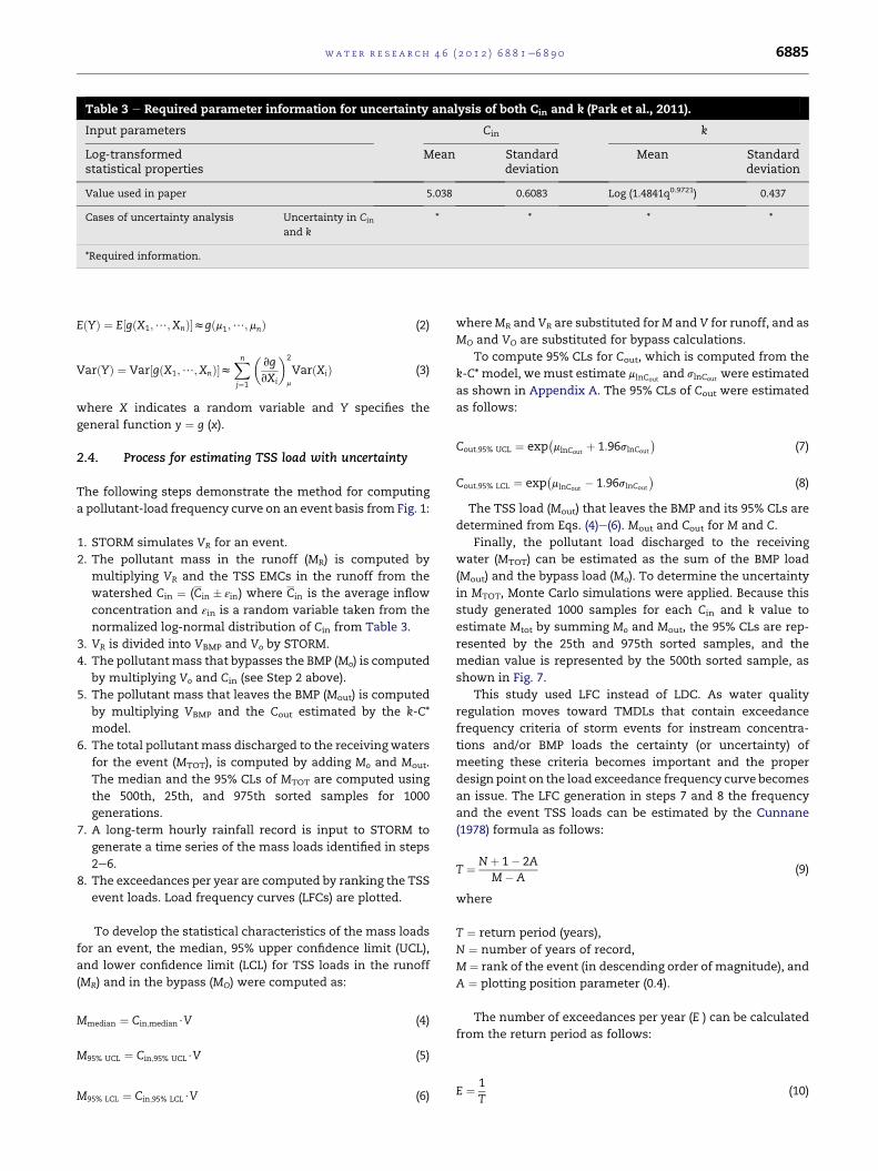
Table 3 e Required parameter information for uncertainty analysis of both Cin and k (Park et al., 2011).

Input parameters Cin k

Log-transformedstatistical properties

Mean Standarddeviation

Mean Standarddeviation

Value used in paper 5.038 0.6083 Log (1.4841q0.9721) 0.437

Cases of uncertainty analysis Uncertainty in Cin

and k

* * * *

*Required information.

wat e r r e s e a r c h 4 6 ( 2 0 1 2 ) 6 8 8 1e6 8 9 0 6885

EðYÞ ¼ E½gðX1;/;XnÞ�zgðm1;/;mnÞ (2)

VarðYÞ ¼ Var½gðX1;/;XnÞ�zXnj¼1

�vgvXi

�2

m

VarðXiÞ (3)

where X indicates a random variable and Y specifies the

general function y ¼ g (x).

2.4. Process for estimating TSS load with uncertainty

The following steps demonstrate the method for computing

a pollutant-load frequency curve on an event basis from Fig. 1:

1. STORM simulates VR for an event.

2. The pollutant mass in the runoff (MR) is computed by

multiplying VR and the TSS EMCs in the runoff from the

watershed Cin ¼ (Cin � εin) where Cin is the average inflow

concentration and εin is a random variable taken from the

normalized log-normal distribution of Cin from Table 3.

3. VR is divided into VBMP and Vo by STORM.

4. The pollutantmass that bypasses the BMP (Mo) is computed

by multiplying Vo and Cin (see Step 2 above).

5. The pollutant mass that leaves the BMP (Mout) is computed

by multiplying VBMP and the Cout estimated by the k-C*

model.

6. The total pollutant mass discharged to the receiving waters

for the event (MTOT), is computed by adding Mo and Mout.

The median and the 95% CLs of MTOT are computed using

the 500th, 25th, and 975th sorted samples for 1000

generations.

7. A long-term hourly rainfall record is input to STORM to

generate a time series of the mass loads identified in steps

2e6.

8. The exceedances per year are computed by ranking the TSS

event loads. Load frequency curves (LFCs) are plotted.

To develop the statistical characteristics of the mass loads

for an event, the median, 95% upper confidence limit (UCL),

and lower confidence limit (LCL) for TSS loads in the runoff

(MR) and in the bypass (MO) were computed as:

Mmedian ¼ Cin;median$V (4)

M95% UCL ¼ Cin;95% UCL$V (5)

M95% LCL ¼ Cin;95% LCL$V (6)

whereMR and VR are substituted forM and V for runoff, and as

MO and VO are substituted for bypass calculations.

To compute 95% CLs for Cout, which is computed from the

k-C* model, wemust estimate mlnCoutand slnCout

were estimated

as shown in Appendix A. The 95% CLs of Cout were estimated

as follows:

Cout;95% UCL ¼ exp�mlnCout

þ 1:96slnCout

�(7)

Cout;95% LCL ¼ exp�mlnCout

� 1:96slnCout

�(8)

The TSS load (Mout) that leaves the BMP and its 95% CLs are

determined from Eqs. (4)e(6). Mout and Cout for M and C.

Finally, the pollutant load discharged to the receiving

water (MTOT) can be estimated as the sum of the BMP load

(Mout) and the bypass load (Mo). To determine the uncertainty

in MTOT, Monte Carlo simulations were applied. Because this

study generated 1000 samples for each Cin and k value to

estimate Mtot by summing Mo and Mout, the 95% CLs are rep-

resented by the 25th and 975th sorted samples, and the

median value is represented by the 500th sorted sample, as

shown in Fig. 7.

This study used LFC instead of LDC. As water quality

regulation moves toward TMDLs that contain exceedance

frequency criteria of storm events for instream concentra-

tions and/or BMP loads the certainty (or uncertainty) of

meeting these criteria becomes important and the proper

design point on the load exceedance frequency curve becomes

an issue. The LFC generation in steps 7 and 8 the frequency

and the event TSS loads can be estimated by the Cunnane

(1978) formula as follows:

T ¼ Nþ 1� 2AM�A

(9)

where

T ¼ return period (years),

N ¼ number of years of record,

M ¼ rank of the event (in descending order of magnitude), and

A ¼ plotting position parameter (0.4).

The number of exceedances per year (E ) can be calculated

from the return period as follows:

E ¼ 1T

(10)

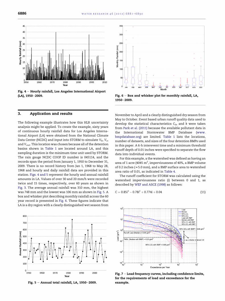
Fig. 4 e Hourly rainfall, Los Angeles International Airport

(LA), 1950e2009. Fig. 6 e Box and whisker plot for monthly rainfall, LA,

1950e2009.

wat e r r e s e a r c h 4 6 ( 2 0 1 2 ) 6 8 8 1e6 8 9 06886

3. Application and results

The following example illustrates how this HLR uncertainty

analysis might be applied. To create the example, sixty years

of continuous hourly rainfall data for Los Angeles Interna-

tional Airport (LA) were obtained from the National Climate

Data Center (NCDC) and input into STORM to simulate VR, Vo,

andVout. This locationwas chosen because all of the detention

basins shown in Table 1 are located around LA, and this

sampling duration is the minimum time unit used by STORM.

The rain gauge NCDC COOP ID number is 045114, and the

records span the period from January 1, 1950 to December 31,

2009. There is no record history from Jan 1, 1968 to May 28,

1968 and hourly and daily rainfall data are provided in this

station. Figs. 4 and 5 represent the hourly and annual rainfall

amounts in LA. Values of over 30 and 20 mm/h were recorded

twice and 15 times, respectively, over 60 years as shown in

Fig. 3. The average annual rainfall was 310 mm, the highest

was 748 mm and the lowest was 106 mm as shown in Fig. 5. A

box andwhisker plot describingmonthly rainfall across the 60

year record is presented in Fig. 6. These figures indicate that

LA is a dry regionwith a clearly distinguishedwet season from

Fig. 5 e Annual total rainfall, LA, 1950e2009.

November to April and a clearly distinguished dry season from

May to October. Event based urban runoff quality data used to

develop the statistical characteristics Cin and k were taken

from Park et al. (2011) because the available pollutant data in

the International Stormwater BMP Database (www.

bmpdatabase.org) are limited. Table 1 lists the locations,

number of datasets, and sizes of the four detention BMPs used

in this paper. A 6-h interevent time and aminimum threshold

runoff depth of 0.01 inches were specified to separate the flow

data into individual events.

For this example, a thewatershedwas defined as having an

area of 1 acre (4045 m2, imperviousness of 40%, a BMP volume

of 0.2 inches (z5.0 mm), and a BMP surface area to watershed

area ratio of 0.01, as indicated in Table 4.

The runoff coefficient for STORM was calculated using the

watershed imperviousness ratio (i) between 0 and 1, as

described by WEF and ASCE (1998) as follows:

C ¼ 0:85i3 � 0:78i2 þ 0:774iþ 0:04 (11)

Fig. 7 e Load frequency curves, including confidence limits,

for the requirements of load and exceedance for the

example.

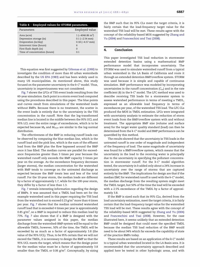
Table 4 e Employed values for STORM parameters.

Parameters Employed value

Area (acre) 1 (¼4046.86 m2)

Depression storage (in) 0.1 (¼2.54 mm)

Evaporation (in/day) 0.18 (¼4.57 mm)

Interevent time (hours) 6

First flush depth (in) 0

Time of concentration (hours) 0.1

wat e r r e s e a r c h 4 6 ( 2 0 1 2 ) 6 8 8 1e6 8 9 0 6887

This equation was first suggested by Urbonas et al. (1990) to

investigate the condition of more than 60 urban watersheds

described by the US EPA (1983) and has been widely used in

many US municipalities. As mentioned above, this study

focused on the parameter uncertainty in the k-C* model. Thus,

uncertainty in imperviousness was not considered.

Fig. 7 shows the LFCs of TSS event loads resulting from the

60-year simulation. Each point is a storm event load computed

using the procedures described in this paper. The blue points

and curves result from simulations of the watershed loads

without BMPs. Because there is no treatment, the scatter in

the event loads is entirely due to the uncertainty in the TSS

concentration in the runoff. Note that the log-transformed

median line is located in themiddle between the 95% UCL and

95% LCL over the entire range of exceedances, which is to be

expected because MR and MTOT are similar to the log-normal

distribution.

The effectiveness of the BMP in reducing runoff loads can

be observed by comparing the blue median line, which is the

runoff load and the pink line, which is the sum of the effluent

load from the BMP plus the flow bypassed around the BMP

once it has filled. The median curves are parallel for exceed-

ance frequencies greater than 3 times per year because the

watershed runoff only exceeds the BMP capacity 3 times per

year on the average. As the exceedance frequency decreases

(larger storms), the median concentration for the watershed

with BMP tends to converge on the untreated discharge as

expected because the BMP treats less and less of the total

runoff. For the 10-year storm, the median loads are different

by a factor of approximately 1.7, while for the 100-year storm,

they differ by a factor of less than 1.3.

Fig. 7 reveals interesting information regarding the design

of BMPs. It was assumed that a TMDL had been set for the

example watershed used in this paper requiring the TSS load

from the watershed not to exceed 0.23 g/m2 more than 4 times

per year. Fig. 7 shows that the median untreated watershed

runoff load that is exceeded 4 times per year is approximately

0.85 g/m2, so a BMP is required to reduce this median load by

73%. Fig. 7 also shows that if a BMP is designed with the

parameter values assigned in this paper, the median

discharge from thewatershed-BMP systemwill be equal to the

allowable TMDL; however, 50% of the time, the TMDL will be

exceeded by as much as a factor of approximately 3.8 (the

value of the 95% UCL). Thus, to be 95% certain that we will not

exceed the TMDL, it is necessary to design the BMP so that the

95% UCL meets the target, which means that the design point

for the median value must be a factor of approximately 3.8

smaller than the TMDL or 0.06 g/m2. Conceptually, by sizing

the BMP such that its 95% CLs meet the target criteria, it is

fairly certain that the load-frequency target value for the

watershed TSS load will be met. These results agree with the

concept of the reliability-based MOS suggested by Zhang and

Yu (2004) and Franceschini and Tsai (2008).

4. Conclusion

This paper investigated TSS load reduction in stormwater

extended detention basins using a mathematical BMP

performance model that incorporates uncertainty. The

STORM was used to simulate watershed runoff from a typical

urban watershed in the LA Basin of California and route it

through an extended detention BMP/overflow system. STORM

was used because it is simple and capable of continuous

simulation. BMP performance was modeled by incorporating

uncertainties in the runoff concentration (Cin) and in the rate

coefficient (k) in the k-C* model. The LFC method was used to

describe receiving TSS loads for a stormwater system to

assess watershed performance in terms of meeting a TMDL,

expressed as an allowable load frequency in terms of

exceedances per year, of the watershed TSS load. The LFC CLs

produced the MOS in TMDL estimation. LFCs were integrated

with uncertainty analysis to estimate the reduction of storm

event loads from the BMP/overflow system with and without

treatment. The appropriate BMP size (volume and surface

area) for the target water quality standard (load) can then be

determined from the k-C* model and BMP performance can be

quantified by this method.

The results showed that the uncertainty in TSS loads in the

untreated runoff is one order of magnitude and independent

of the frequency of load. The same magnitude of uncertainty

was found for a BMP/overflow system, which means that the

uncertainty in the load to the receiving water is principally

due to the uncertainty in specifying the pollutant concentra-

tion in stormwater runoff. For the k-C* model algorithm

tested, the uncertainty in k added only about a 24% increase in

uncertainty over the range of storms that are captured

entirely by the BMP. The implications for design are that if the

median EMC for watershed runoff is used with the k-C* model,

the median discharge from the resulting system might meet

the TMDL target, but 50% of the time the load will be exceeded

with a 2.5% exceedance of the TMDL by a factor of approxi-

mately 3.8.

If the BMP is sized such that its 95% CLs, derived from the

load uncertainty estimation,meet the target criteria, it is fairly

certain that the load-frequency target value for the watershed

TSS load will be met. These results agree with the concept of

the reliability-based MOS suggested by Zhang and Yu (2004)

and Franceschini and Tsai (2008). However, for the case

illustrated here, it seems unlikely that an extended detention

BMP could be designed that could meet the specified TMDL

because the median TSS load reduction of the BMP would

need to be about 94% which far exceeds the capability of state

of the practice BMPs today.

These results are based on an application of the k-C* model

to a typical urban watershed located in the LA Basin area. It is

recommended that the uncertainty approach described and

applied here be tested in other hydrologic areas, and with

wat e r r e s e a r c h 4 6 ( 2 0 1 2 ) 6 8 8 1e6 8 9 06888

different BMP algorithms, which may yield better results. It

seems certain that sizing BMPs based on median EMCs of

runoff will not provide reliable pollutant removal from

stormwater discharges to receiving waters.

Appendix A. Derivation of mlnCoutand slnCout

First, it is necessary to log-transform the original EMC data. x

represents an element of the original EMC data and y repre-

sents its respective log-transformed result as described below,

assuming that the data are normally distributed.

y ¼ lnðxÞ (12)

The mean (mx) and standard deviation (sx) of the log-normal

EMC distribution are related to the log-transformed mean (my)

and standard deviation (sy) by the method of moments as

follows (Salas et al., 2004):

mx;median ¼ exp�my

�(13)

mx ¼ exp

my þ

s2y

2

!(14)

s2x ¼

nexp

�s2y

�� 1oexp

�2my þ s2

y

�(15)

my ¼12ln

0B@ m2

x

1þ�sx

mx

�2

1CA (16)

s2y ¼ ln

�1þ

�sx

mx

�2�(17)

where

mx ¼ the mean of the EMC data,

sx ¼ the standard deviation of the EMC data,

mx;median ¼ the median of the EMC data,

my ¼ the mean of the log-transformed EMC data, and

sy ¼ the standard deviation of the log-transformed EMC data.

Only the bypass-overflow volume is needed because the

pollutant concentration is assumed to be equal to Cin. The

effluent pollutant concentration in the BMP (Cout) is calculated

as the estimated pollutant concentration from the k-C* model

as follows:

mlnCout¼ ln

�Cout;median

�¼ ln

�C� þ �Cin;median � C��$expð�kmedian=qÞ

(18)

If Cout,median is log-transformed, it becomes the mean of the

log-transformed values and is called mlnCout. The standard

deviation of k can be calculated from the log-transformed

mean and standard deviation from Eq. (15), as follows:

sk ¼ffiffiffiffiffiffiffiffiffiffiffiffiffiffiffiffiffiffiffiffiffiffiffiffiffiffiffiffiffiffiffiffiffiffiffiffiffiffiffiffiffiffiffiffiffiffiffiffiffiffiffiffiffiffiffiffiffiffiffiffiffiffiffiffiffiffiffiffiffiffiffiffiffiffi�exp

�s2lnk

�� 1$exp

�2mlnk þ s2

lnk

�q(19)

It is assumed that Cin and k are independent. Therefore, the

standard deviation of Cout can be evaluated using Eqs. (1) and

(3), respectively, as follows:

scout ¼�expð�kmedian=qÞ2$s2

Cin

þ��

Cin;median � C��q

expð�kmedian=qÞ 2

$s2k

�1=2 (20)

Using Eq. (16), themean value of Cout (mCout) can be estimated

as follows:

mCout¼

ffiffiffiffiffiffiffiffiffiffiffiffiffiffiffiffiffiffiffiffiffiffiffiffiffiffiffiffiffiffiffiffiffiffiffiffiffiffiffiffiffiffiffiffiffiffiffiffiffiffiffiffiffiffiffiffiffiffiffiffiffiffiffiffiffiffiffiffiffiffiffiffiffiffiffiffiffiffiffiffiffiffiffiffiffiffiffiffiffiffiffiffiffiffiffiffiffiffiffiffiffiffiffiffiffiffiffiffiffiffiffiffiffiffiffiffiffiexp

�2mlnCout

�þ ffiffiffiffiffiffiffiffiffiffiffiffiffiffiffiffiffiffiffiffiffiffiffiffiffiffiffiffiffiffiffiffiffiffiffiffiffiffiffiffiffiffiffiffiffiffiffiffiffiffiffiffiffiffiffiffiffiffiffiffiffiffiffiffiffiffiffiffiffiffiffiffiffiffiffiffiffiffi�exp

�4mlnCout

�þ 4s2Cout

exp�2mlnCout

��q2

vuut(21)

The log-transformed standard deviation of Cout can be

determined by combining Eq. (17) with Eqs. (20) and (21) as

follows:

slnCout ¼�ln

�1þ

�sCout

mCout

�2 �1=2(22)

r e f e r e n c e s

Adams, B.J., Papa, F., 2000. Urban Stormwater ManagementPlanning with Analytical Probabilistic Models. Wiley, NewYork, NY, USA.

Arabi, M., Govindaraju, R.S., Hantush, M.M., 2007. A probabilisticapproach for analysis of uncertainty in the evaluation ofwatershed management practices. Journal of Hydrology 333(2e4), 459e471.

Barrett, M.E., 2005. Performance comparison of structuralstormwater best management practices. Water EnvironmentResearch 77 (1), 78e86.

Bonta, J.V., Cleland, B., 2003. Incorporating natural variability,uncertainty, and risk into water quality evaluations usingduration curves. Journal of the American Water ResourcesAssociation 39 (6), 1481e1496.

Braskerud, B.C., 2002. Factors affecting phosphorus retention insmall constructed wetlands treating agricultural non-pointsource pollution. Ecological Engineering 19 (1), 41e61.

Burges, S.J., Lettenmaier, D.P., 1975. Probabilistic methods instream quality management. Water Resources Bulletin 11 (1),115e130.

Carleton, J.N., Montas, H.J., 2007. A modeling approach for mixingand reaction in wetlands with continuously varying flow.Ecological Engineering 29 (1), 33e44.

Carleton, J.N., 2002. Damkohler number distributions andconstituent removal in treatment wetlands. EcologicalEngineering 19 (4), 233e248.

California Stormwater Quality Assoication (CASQA), 2003.Stormwater Best Management Practic Handbook: NewDevelopment and Redevelopment. California StormwaterQuality Association.

Cleland, B., 2002. TMDL development from the “bottom up” e

part II: using duration curves to connect the pieces. In:Proceedings of National TMDL Science and PolicyConference. Water Environment Federation, Phoenix, AZ,USA.

Cleland, B., 2003. TMDL development from the “bottom up”ePart III: duration curves and wet-weather assessments. In:Proceedings of National TMDL Science and PolicyConference. Water Environment Federation, Chicago, IL,USA.

wat e r r e s e a r c h 4 6 ( 2 0 1 2 ) 6 8 8 1e6 8 9 0 6889

Crites, R.W., Reed, S.C., Middlebrooks, E.J., 2006. NaturalWastewater Treatment Systems. CRC/Taylor & Francis, BocaRaton, FL, USA.

Cunnane, C., 1978. Unbiased plotting positions e A review.Journal of Hydrology 37 (3e4), 205e222.

D’Agostino, R.B., Stephens, M.A., 1986. Goodness-of-fitTechniques. Marcel Dekker, New York, NY.

Dotto, C.B.S., Kleidorfer, M., Deletic, A., Rauch, W.,McCarthy, D.T., Fletcher, T.D., 2011. Performance andsensitivity analysis of stormwater models using a Bayesianapproach and long-term high resolution data. EnvironmentalModelling & Software 26 (10), 1225e1239.

Franceschini, S., Tsai, C.W., 2008. Incorporating reliability into thedefinition of the margin of safety in total maximum daily loadcalculations. Journal of Water Resources Planning andManagement 134 (1), 34e44.

Heineman, M.C., 2004. NetSTORM e a computer program forrainfall-runoff simulation and precipitation analysis. In:Proceedings of the World Water and Environmental ResourcesCongress. ASCE, Salt Lake City, UT, USA.

Huber, W.C., 2006. BMP Modeling Concepts and Simulation. USEPA, Corvallis, OR, USA.

Kadlec, R.H., Knight, R.L., 1996. Treatment Wetlands. CRC LewisPublishers, Boca Raton, FL, USA.

Kadlec, R.H., Reddy, K.R., 2001. Temperature effects in treatmentwetlands. Water Environment Research 73 (5), 543e557.

Kadlec, R.H., 2000. The inadequacy of first-order treatmentwetland models. Ecological Engineering 15 (1e2), 105e119.

Kadlec, R.H., 2003. Effects of pollutant speciation in treatmentwetlands design. Ecological Engineering 20 (1), 1e16.

Kleidorfer, M., Deletic, A., Fletcher, T.D., Rauch, W., 2009.Impact of input data uncertainties on urban stormwatermodel parameters. Water Science and Technology 60 (6),1545e1554.

Kottegoda, N.T., Rosso, R., 1997. Statistics, Probability, andReliability for Civil and Environmental Engineers. McGraw-Hill, New York, NY, USA.

Lee, J.G., Heaney, J.P., Lai, F.H., 2005. Optimization of integratedurban wet-weather control strategies. Journal of WaterResources Planning and Management 131 (4), 307e315.

Lin, Y.F., Jing, S.R., Lee, D.Y., Chang, Y.F., Chen, Y.M., Shih, K.C.,2005. Performance of a constructed wetland treating intensiveshrimp aquaculture wastewater under high hydraulic loadingrate. Environmental Pollution 134 (3), 411e421.

Melching, C.S., Anmangandla, S., 1992. An improved 1st-orderuncertainty method for water-quality modeling. Journal ofEnvironmental Engineering 118 (5), 791e805.

Minton, G.R., 2005. Stormwater Treatment: Biological, Chemical,and Engineering Principles, second ed. Resource PlanningAssociates, Seattle, WA, USA.

Nix, S.J., Heaney, J.P., 1988. Optimization of storm water storage-release strategies. Water Resources Research 24 (11),1831e1838.

O’Donnell, K.J., Tyler, D.F., Wu, T.S., 2005. TMDL report: fecal andtotal coliform TMDL for the new river, (WBID 1442). In:Proceedings of the 3rd Conference of Watershed Managementto Meet Water Quality Standards and Emerging TMDL.Atlanta, GA, USA.

Park, D., Loftis, J.C., Roesner, L.A., 2011. Modeling performance ofstorm water best management practices with uncertaintyanalysis. Journal of Hydrologic Engineering 16 (4), 332e344.

Park, D., Song, Y.-I., Roesner, L.A., in press. The effect of theseasonal rainfall distribution on storm-water quality capturevolume estimation. Journal of Water Resources Planning andManagement.

Patry, G.G., Kennedy, A., 1989. Pollutant washoff under noise-corrupted runoff conditions. Journal of Water ResourcesPlanning and Management 115 (5), 646e657.

Roesner, L.A., Nichandros, H.M., Shubinski, R.P., Feldman, A.D.,Abbott, J.W., Friedland, A.O., 1974. A Model for EvaluatingRunoff-quality in Metropolitan Master Planning. TechnicalMemorandum No.23 (NTIS PB-234312). ASCE Urban WaterResources Research Program, New York, NY, USA.

Roesner, L.A., 1982. Chapter 5 Quality of Urban Runoff e UrbanStorm Water Hydrology (Water Resources Monograph 6).American Geophysical Union, Washington DC, USA.

Rousseau, D.P.L., Vanrolleghem, P.A., De Pauw, N., 2004. Model-based design of horizontal subsurface flow constructedtreatment wetlands: a review. Water Research 38 (6),1484e1493.

Salas, J.D., Smith, R.A., Tabious, G.Q., Heo, J.-H., 2004. StatisticalTechniques inWater ResourcesandEnvironmental Engineering.Colorado State University, Fort Collins, Colorado, USA.

Schierup, H., Brix, H., Lorenzen, B., 1990. Wastewater Treatmentin Constructed Reed Beds in DenmarkeState of the Art.Constructed Wetlands in Water Pollution Control. PergamonPress, London, UK.

Schueler, T.R., 1996. Irreducible pollutant concentrationsdischarged from stormwater practices. Technical Note 75.Watershed Protection Techniques 2 (2), 369e372.

Segarra-Garcia, R., Basha-Rivera, M., 1996. Optimal estimation ofstorage-release alternatives for storm-water detentionsystems. Journal of Water Resources Planning andManagement 122 (6), 428e436.

Segarra-Garcia, R., Loganathan, V.G., 1992. Storm-water detentionstorage design under random pollutant loading. Journal ofWater Resources Planning and Management 118 (5), 475e491.

Shen, J., Zhao, Y., 2010. Combined Bayesian statistics and loadduration curve method for bacteria nonpoint source loadingestimation. Water Research 44 (1), 77e84.

Shirmohammadi, A., Chaubey, I., Harmel, R.D., Bosch, D.D.,Munoz-Carpena, R., Dharmasri, C., Sexton, A., Arabi, M.,Wolfe, M.L., Frankenberger, J., Graff, C., Sohrabi, T.M., 2006.Uncertainty in TMDL models. Transactions of the ASABE 49(4), 1033e1049.

Song, Q., Brown, L.C., 1990. Do model uncertainty with correlatedinputs. Journal of Environmental Engineering 116 (6), 1164e1180.

Stiles, T.C., 2001. A simple method to define bacteria TMDLs inKansas. In: Proceedings of TMDL Science Issues Conferences.Water Environment Federation and Association of State andInterstate Water Pollution Control Administrators,Alexandria, VA and Washington, D.C., USA.

Tung, Y.K., Hathhorn, W.E., 1988. Assessment of probability-distribution of dissolved-oxygen deficit. Journal ofEnvironmental Engineering 114 (6), 1421e1435.

Tung, Y.K., Mays, L.W., 1981. Risk models for flood levee design.Water Resources Research 17 (4), 833e841.

Urbonas, B.R., Guo, J.C.Y., Tucker, L.S., 1990. Optimization ofstormwater quality capture volume. In: Proceedings of UrbanStormwater Quality Enhancement-Source Control, Retrofittingand Combined Sewer Technology. ASCE, New York, NY, USA.

US Army Corps of Engineers, 1977. Storage, Treatment, Overflow,Runoff Model “STORM” User’s Manual. CPD-7. HydrologicEngineering Center, Davis, CA, USA.

US Environmental Protection Agency (US EPA), 1983. Final Report.Results of the Nationwide Urban Runoff Program, vol. 1. WaterPlanning Division, Washington, DC, USA.

US Environmental Protection Agency (US EPA), 2007. An Approachfor Using Load Duration Curves in the Development of TMDLs.US EPA, Washington, DC, USA.

Water Environment Federation (WEF), American Society of CivilEngineers (ASCE), 1998. Urban Runoff Quality Management-MOP 23. Water Environment Federation, Alexandria, VA, USA.

Wong, T.H.F., Geiger, W.F., 1997. Adaptation of wastewatersurface flow wetland formulae for application in constructedstormwater wetlands. Ecological Engineering 9 (3e4), 187e202.

wat e r r e s e a r c h 4 6 ( 2 0 1 2 ) 6 8 8 1e6 8 9 06890

Wong, T.H.F., Fletcher, T.D., Duncan, H.P., Coleman, J.R.,Jenkins, G.A., 2002. A model for urban stormwaterimprovement conceptualization. In: The 9th InternationalConference on Urban Drainage. ASCE, Portland, OR, USA.

Wong, T.H.F., Fletcher, T.D., Duncan, H.P., Jenkins, G.A., 2006.Modelling urban stormwater treatment - a unified approach.Ecological Engineering 27 (1), 58e70.

Yen, B.C., Tang, W.H., 1976. Risk-safety factor relation for stormsewer design. Journal of the Environmental EngineeringDivision 102 (2), 509e516.

Zhang, H.X., Yu, S.L., 2004. Applying the first-order error analysisin determining the margin of safety for total maximum dailyload computations. Journal of Environmental Engineering 130(6), 664e673.