Evaluation of Material Models to Predict Material Failure ...

Department of Construction Sciences

Solid Mechanics

ISRN LUTFD2/TFHF-16/5209-SE(1-55)

Evaluation of Material Models toPredict Material Failure in LS-DYNA

Master’s Dissertation by

Hjalmar SandbergOscar Rydholm

Supervisors:Johan Hektor, Div. of Solid Mech. LTH

Niclas Brannberg, CEVT AB

Examiner:Matti Ristinmaa, Div. of Solid Mech. LTH

Copyright c© 2016 by the Division of Solid Mechanicsand Hjalmar Sandberg & Oscar Rydholm

Printed by Media-Tryck AB, Lund, SwedenFor information, address:

Division of Solid Mechanics, Lund University, Box 118, SE-221 00 Lund, SwedenWebpage: www.solid.lth.se

Abstract

Computer simulation of car crashes is an important tool in the car development pro-cess. With increased awareness of the environment, it is important that the excessof material usage for the car is minimized. The effect of the material reduction mustnot compromise the safety of the passengers. It is possible to use computer simula-tions for the reduced structure at a certain loading to see how the crashworthiness isaffected. To be able to rely on the simulated result, it is necessary to have a materialmodel that predicts the material behaviour accurately. CEVT is currently using anadvanced material model called MF GenYld+CrachFEM 1. The main drawbacks ofthis model are that it affect the simulation time in a high extent and it also requiresan additional license cost.

The objective of the thesis is to implement a new material model and compare itto the current one. The material model that is considered is implemented within LS-DYNA and works as a combination of an elasto-plastic model called *MAT 024 anda failure model called GISSMO. The implementation requires the user to define a setof material parameters. To obtain these a characterization of the material is neededand since no experimental data is available for this thesis, this is done by simulatedmaterial tests where the material behaviour is modelled with MF GenYld+CrachFEM.

The two material models are compared during two complex load cases, one depictinga B-pillar2 and one depicting a rear bumper crash. The two material models proveto have similar results, but the simulation with *MAT 024 and GISSMO reduce thesimulation time extensively.

1The material model MF GenYld+CrachFEM is often referred to as just CrachFEM.2Pillar located between the front- and the back door of a car.

Acknowledgement

The Master Thesis was carried out at CEVT in Gothenburg in cooperation with theDivision of Solid Mechanics at Lund University. It was initiated in January 2016 andcompleted in June 2016.

Firstly, we would like to thank our supervisor at CEVT, Niclas Brannberg, for hispatience and valuable discussions during the process. Secondly, we would like to givea special thanks to our supervisor at LTH, Johan Hektor, for his feedback and valu-able support during the project. We would like to thank our colleagues at CEVTfor making our stay pleasant. Finally, an extra thanks to Hans Merkle at CEVT andMikael Schill at DYNAmore for helping us with theoretical and practical issues duringthe thesis.

Lund, June 2016Oscar Rydholm and Hjalmar Sandberg

Contents

1 Introduction 11.1 China Euro Vehicle Technology AB (CEVT) . . . . . . . . . . . . . . . 11.2 Background . . . . . . . . . . . . . . . . . . . . . . . . . . . . . . . . . 11.3 Objective . . . . . . . . . . . . . . . . . . . . . . . . . . . . . . . . . . 2

2 Theory 32.1 Stress measures . . . . . . . . . . . . . . . . . . . . . . . . . . . . . . . 32.2 Material testing . . . . . . . . . . . . . . . . . . . . . . . . . . . . . . . 3

2.2.1 Uniaxial tension test . . . . . . . . . . . . . . . . . . . . . . . . 32.2.2 Standardized material test . . . . . . . . . . . . . . . . . . . . . 5

2.3 Strain rate dependency . . . . . . . . . . . . . . . . . . . . . . . . . . . 62.4 Damage mechanics . . . . . . . . . . . . . . . . . . . . . . . . . . . . . 72.5 Explicit analysis . . . . . . . . . . . . . . . . . . . . . . . . . . . . . . . 8

3 Material modelling 103.1 LS-DYNA . . . . . . . . . . . . . . . . . . . . . . . . . . . . . . . . . . 10

3.1.1 *MAT 024 . . . . . . . . . . . . . . . . . . . . . . . . . . . . . . 103.1.2 *MAT ADD EROSION . . . . . . . . . . . . . . . . . . . . . . 10

3.2 LS-OPT . . . . . . . . . . . . . . . . . . . . . . . . . . . . . . . . . . . 113.3 Material failure . . . . . . . . . . . . . . . . . . . . . . . . . . . . . . . 11

3.3.1 MF GenYld+CrachFEM . . . . . . . . . . . . . . . . . . . . . . 123.3.2 GISSMO . . . . . . . . . . . . . . . . . . . . . . . . . . . . . . . 15

4 Results 174.1 CrachFEM results . . . . . . . . . . . . . . . . . . . . . . . . . . . . . . 17

4.1.1 Test specimen validation . . . . . . . . . . . . . . . . . . . . . . 174.1.2 Results from uniaxial tension test . . . . . . . . . . . . . . . . . 184.1.3 Results from notch and shear tests . . . . . . . . . . . . . . . . 20

4.2 *MAT 024 results . . . . . . . . . . . . . . . . . . . . . . . . . . . . . . 214.2.1 Results from uniaxial tension test . . . . . . . . . . . . . . . . . 21

4.3 LS-OPT results . . . . . . . . . . . . . . . . . . . . . . . . . . . . . . . 224.3.1 Result from uniaxial tension test . . . . . . . . . . . . . . . . . 224.3.2 Results from notch and shear tests . . . . . . . . . . . . . . . . 244.3.3 Instability and failure calibration . . . . . . . . . . . . . . . . . 264.3.4 Regularization of element size . . . . . . . . . . . . . . . . . . . 27

4.4 GISSMO results . . . . . . . . . . . . . . . . . . . . . . . . . . . . . . . 294.4.1 B-Pillar . . . . . . . . . . . . . . . . . . . . . . . . . . . . . . . 294.4.2 Rear crash . . . . . . . . . . . . . . . . . . . . . . . . . . . . . . 34

5 Analysis 38

6 Conclusions 40

7 Appendix 437.1 Test specimens . . . . . . . . . . . . . . . . . . . . . . . . . . . . . . . 437.2 B-Pillar . . . . . . . . . . . . . . . . . . . . . . . . . . . . . . . . . . . 457.3 Rear crash . . . . . . . . . . . . . . . . . . . . . . . . . . . . . . . . . . 46

1 INTRODUCTION 1

1 Introduction

1.1 China Euro Vehicle Technology AB (CEVT)

CEVT was founded in mid 2013 as a R&D center for the platform3 of the C-segment4

cars of Geely Group. CEVT has expanded from nine people to approximately 1500 atpresent time. Nowadays, the company is active as a subcontractor to Volvo Cars andGeely, where they still are working with the car platform and can also offer expertisewith complete vehicle design. CEVTs offices are located in Gothenburg, Sweden andHangzhou, China.

1.2 Background

Due to the global trend to reduce CO2 emissions from vehicles, focus is pointed atdecreasing the weight of the car. A demanding issue is to decrease the weight and stilllet the crashworthiness be remained. One way of examining the opportunities of thisis to simulate the car’s behaviour during a crash. Thereby, it is possible to estimatehow the changes in structure affect the crashworthiness. However, to be able to usethe simulated results as guidance, there are some factors that needs to be considered.The first step to make the simulation reliable, is to model the material behaviouraccurately. Andrade, Feucht and Haufe [1] have flagged for another factor, there is aninformation gap between the forming process and crash analysis where important datais lost between the different development stages. An interest of closing the gap hasarisen, since the forming operations may affect the crashworthiness of the producedparts. Another trend that Effelsberg et al. [7] claim, is that the new material modelstry to predict the actual failure behaviour, instead of just describing the initiation ofmaterial failure which have been the case earlier.

To be able to consider material failure in simulations, CEVT is currently using theproprietary material models from Crachfem by Matfem. These material models, whichare based on an extensive set of material tests, can handle a number of different ma-terial models. Unfortunately, the simulation configuration for Crachfem is encrypted,which means that the input parameters are hidden and the whole model may beviewed as a black box.

The thesis project is of interest for CEVT since there are a few other drawbacksof CrachFEM. Firstly, the material model itself takes a substantial amount of timeto process, and hence, it is slowing down the simulations. Secondly, the additionallicense cost for CrachFEM is high.

3A car platform is the under body of the car and the device that everything is attached to.4The C-segment is a car classification that is done with respect to the car’s size. It includes cars

like Volkswagen Golf and Ford Focus.

1 INTRODUCTION 2

1.3 Objective

This thesis shall evaluate a material failure model called GISSMO, General Incremen-tal Stress-State dependent Damage Model, [13] and compare it with CrachFEM. Theimplementation of GISSMO require characteristic properties for the material used.To obtain these properties, a variety of material tests have to be performed. Thisproject does not cover physical material tests and no experimental data are available.Thus, the input parameters for the material model will be generated from numericalsimulations, where CrachFEM is used to model the material failure. To ensure thatthe characterization is done correctly, the thesis starts with a literature study. Thestudy involves how to perform material tests, the theory behind the different mate-rial models and learning about the software that will be used. The specimens to thematerial testing have to be designed, meshed and applied with boundary conditions.This will be done in the software ANSA [17]. The simulations of the material testswill be performed in LS-DYNA [13], which is a solver that is widely used to performfinite element calculations in the automotive industry. These simulations will providethe fundamental material properties needed to implement GISSMO. Before the prop-erties can be implemented, they need to be calibrated through reversed engineeringwith help of an optimization tool. This project will use a software called LS-OPT[4] to perform the optimization. When the new material model is implemented, itis to be compared with CrachFEM. The comparison will be done with two differentcomplex load cases. The first load case is of a simplified B-pillar. This test will pri-marily measure the difference in simulation time between the models and secondarilynotice tendencies of the material’s failure behaviour. During the second load case,the loading is subjected to a car’s rear end and the behaviour of the bumper will beanalyzed. GISSMO’s accuracy will be the primary measurement for this load case.See Figure 43 and 44 to see the geometries of the two cases.

The global objective for this thesis is to find which of the models that are mostsuitable to use in car crash simulations. This is done by evaluating the accuracy ofthe result and the extra amount of time required to run a simulation with differentmaterial models. This report aims to work as guidance when choosing a failure modelfor car crash simulations.

2 THEORY 3

2 Theory

2.1 Stress measures

Bridgman [3], Rice and Trace [16] have showed that material failure is dependent ofthe stress state. Hence, the stress state is necessary to take into consideration whencharacterizing a material’s properties. When performing crashworthiness calculations,it is useful to describe the stress state of different load cases using the invariants ofthe stress tensor. Crashworthiness computations are often performed on a sheet metalstructure and a common assumption for this structure is that plane stress prevails. Ifplane stress prevails, the different stress states can be uniquely determined with justone parameter. The parameter is called the triaxiality, η, and it is defined as

η =I1σeq

(1)

where I1 is the first stress invariant

I1 =σ1 + σ2 + σ3

3(2)

and σeq is the von Mises stress and σ1, σ2, σ3 are the principal stresses.

σeq =√σ21 + σ2

2 + σ23 − σ1σ2 − σ1σ3 − σ2σ3 (3)

Von Mises yield criteria is frequently used when considering materials with isotropicproperties. It is formulated as

F (σ) = σeq − σy(k) (4)

where σy(k) is the yield stress as function of a hardening parameter, k. Yielding occurwhen F (σ) = 0.

2.2 Material testing

To understand what applications a certain material is suitable for, it is necessary tocharacterize its properties. To characterize a material’s failure properties, differentstress states have to be analyzed. This thesis involves analyzing the behaviour duringfive different material tests. These are one uniaxial tension test, two different sheartests and two different notched tests. These different tests are chosen because theycover a wide spectrum of stress states. The geometries of the specimens that are usedin this thesis are visualized in Appendix, see Figure 38-42.

2.2.1 Uniaxial tension test

The most fundamental material properties can be obtained from a uniaxial tensiontest. It is performed by locking one end of the specimen and applying a predefinedload to the other. The elongation of the specimen is measured until failure. With

2 THEORY 4

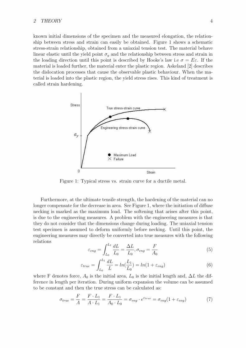
known initial dimensions of the specimen and the measured elongation, the relation-ship between stress and strain can easily be obtained. Figure 1 shows a schematicstress-strain relationship, obtained from a uniaxial tension test. The material behavelinear elastic until the yield point σy and the relationship between stress and strain inthe loading direction until this point is described by Hooke’s law i.e σ = Eε. If thematerial is loaded further, the material enter the plastic region. Askeland [2] describesthe dislocation processes that cause the observable plastic behaviour. When the ma-terial is loaded into the plastic region, the yield stress rises. This kind of treatment iscalled strain hardening.

Figure 1: Typical stress vs. strain curve for a ductile metal.

Furthermore, at the ultimate tensile strength, the hardening of the material can nolonger compensate for the decrease in area. See Figure 1, where the initiation of diffusenecking is marked as the maximum load. The softening that arises after this point,is due to the engineering measures. A problem with the engineering measures is thatthey do not consider that the dimensions change during loading. The uniaxial tensiontest specimen is assumed to deform uniformly before necking. Until this point, theengineering measures may directly be converted into true measures with the followingrelations

εeng =

∫ L1

L0

dL

L0

=∆L

L0

, σeng =F

A0

(5)

εtrue =

∫ L1

L0

dL

L= ln(

L1

L0

) = ln(1 + εeng) (6)

where F denotes force, A0 is the initial area, L0 is the initial length and, ∆L the dif-ference in length per iteration. During uniform expansion the volume can be assumedto be constant and then the true stress can be calculated as:

σtrue =F

A=F · L1

A · L1

=F · L1

A0 · L0

= σeng · eεtrue = σeng(1 + εeng) (7)

2 THEORY 5

where A and L are the current dimensions of the specimen.

The true strain consists of one elastic part and one plastic part. Equation 6 togetherwith Hooke’s law gives the true plastic strain as

εtrue,plast = εtrue −σtrueE

(8)

which is valid until diffused necking occurs i.e at the maximum load. The physical in-terpretation of diffused necking is when the specimen no longer is deformed uniformlyand the specimen suffer from a quick reduction of the width at a certain cross section.

2.2.2 Standardized material test

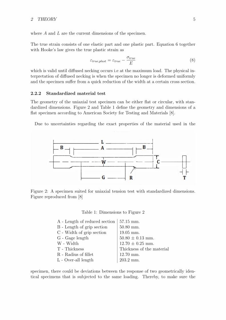
The geometry of the uniaxial test specimen can be either flat or circular, with stan-dardized dimensions. Figure 2 and Table 1 define the geometry and dimensions of aflat specimen according to American Society for Testing and Materials [8].

Due to uncertainties regarding the exact properties of the material used in the

Figure 2: A specimen suited for uniaxial tension test with standardized dimensions.Figure reproduced from [8]

Table 1: Dimensions to Figure 2

A - Length of reduced section 57.15 mm.B - Length of grip section 50.80 mm.C - Width of grip section 19.05 mm.G - Gage length 50.80 ± 0.13 mm.W - Width 12.70 ± 0.25 mm.T - Thickness Thickness of the materialR - Radius of fillet 12.70 mm.L - Over-all length 203.2 mm.

specimen, there could be deviations between the response of two geometrically iden-tical specimens that is subjected to the same loading. Thereby, to make sure the

2 THEORY 6

results are reliable, it is recommended to do a series of tests and compare the results.However, since CEVT has not got any experimental data available at this time, thematerial testing is completely done by computer simulations. The same specimensare used together with the different material models.

2.3 Strain rate dependency

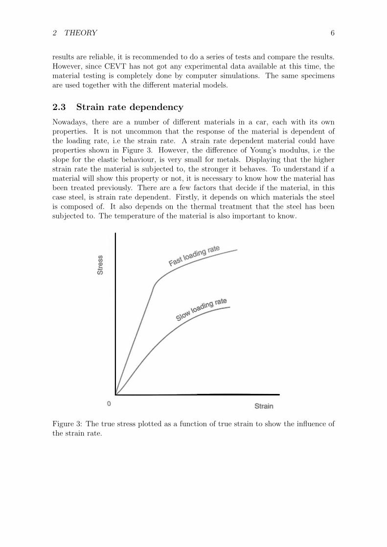
Nowadays, there are a number of different materials in a car, each with its ownproperties. It is not uncommon that the response of the material is dependent ofthe loading rate, i.e the strain rate. A strain rate dependent material could haveproperties shown in Figure 3. However, the difference of Young’s modulus, i.e theslope for the elastic behaviour, is very small for metals. Displaying that the higherstrain rate the material is subjected to, the stronger it behaves. To understand if amaterial will show this property or not, it is necessary to know how the material hasbeen treated previously. There are a few factors that decide if the material, in thiscase steel, is strain rate dependent. Firstly, it depends on which materials the steelis composed of. It also depends on the thermal treatment that the steel has beensubjected to. The temperature of the material is also important to know.

Figure 3: The true stress plotted as a function of true strain to show the influence ofthe strain rate.

2 THEORY 7

2.4 Damage mechanics

Damage is a central part of the material properties when considering material failure.The concept assumes growth of voids in the material. The damage, D, is basicallya measure for the reduction of the cross section area with respect to the upcomingvoids, see Figure 4.

Figure 4: The current section area and the effective section area. Figure reproducedfrom [10].

Figure 4 shows the overall section area including micro defects and the reduced,effective, section area. If A represents the current section area, i.e the cross sectionarea including the area of the voids, and Aeff represents the effective cross sectionarea, i.e. the cross section area excluding the area of the voids, Lemaitre and Chaboche[12] define the damage parameter as follows

D = 1− Aeff

A=Adefect

A(9)

Adefect = A− Aeff (10)

When the damage equals 1, the material fails. The reduction of the cross section hasan effect on the stress used to model the global response. The definition of σtrue, seeequation 7, together with equation 9 above gives Lemaitre’s formulation [12] which isa basic relation to couple damage to the stresses

σeff =F

Aeff

=σtrue

1−D⇒ σtrue = (1−D)σeff (11)

This is basic damage theory and the fundamentals for the different failure models.One common difference between the models is the damage evolution. Liang Xue[19] claims that one of the most commonly used and simplest ways of describing thedamage evolution is the Johnson Cook model that yields

D =εpεf

(12)

where the damage evolution is proportional to the equivalent plastic strain rate, εpand εf is the equivalent plastic strain at failure. Besides this, there are other damageevolution laws that are used e.g. the evolution law used in GISSMO.

2 THEORY 8

2.5 Explicit analysis

To solve time dependent ordinary differential equations (ODE) and partial differentialequations (PDE) with finite element analysis, either an explicit or an implicit methodis used. For example the equation of motion that is given by

Man + fint(an) = fn (13)

where M is the mass matrix, fint(an) is the internal forces, fn is the external forces,an is the displacement, an is the acceleration and index n represent the current timestep where the nodal values is known. The explicit method implies that instead ofsolving for an it solves for an. By doing this, the solving of the inverse of the stiffnessmatrix which is included in fint(an) is avoided. Yang et al. [20] claims that this is anadvantage since solving the inverse could be demanding when considering big systems.

According to Ottosen and Ristinmaa [15], Newmark’s time integration scheme may beused to solve equation 13 for an and the integration scheme reduces to the following:

an+1 = an + an∆t+∆t2

2an (14)

an+1 = an +∆t

2(an + an+1) (15)

where ∆t is the time step and the nodal values with index n are known. With thesetwo equations, it is possible to obtain an expression where a is expressed in terms ofa, see [15] for details.

an =1

∆t2(an+1 − 2an + an−1) (16)

If equation 16 is inserted in equation 13 it is reformulated as

Man+1 = M(2an − an−1) + ∆t2(fn − fint(an)) (17)

Where the nodal values of index n and n-1 are known and the internal forces can bedetermined. Also since explicit method usually use lower order elements, M will bea diagonal matrix, meaning that the inverse of the mass matrix is trivial. Hence, anonlinear dynamic problem as for example, elastic-plastic material behaviour can besolved directly without iterations. However, the simplification has its disadvantage,which is that the solving technique is only conditionally stable. If the solution becomesunstable the error will rapidly increase with every time step and the solution willbecome invalid. An explicit method usually needs to have 100 to 10000 times smallertime steps than an implicit technique, that is unconditionally stable, to avoid thiskind of error. The time step for this method is limited by the time it takes for theshock wave, that arises from the loading, to transmit through the smallest element inthe mesh

∆t =dmin

c(18)

2 THEORY 9

where dmin is the smallest distance between any two nodes in an element and c is thesound speed in the material. The speed of sound is computed as

c =

√E

ρ(1− ν2)(19)

where E is Young’s modulus, ρ is the mass density and ν is Poisson’s ratio. Thesolving method does not allow the shock wave to transmit a longer distance than dmin

during ∆t and regulates this by slowing down the sound speed by increasing the massdensity of this element. Thereby, to prevent the solution for becoming unstable, themass density of the element is raised. See LS-DYNA - theory manual, chapter 22 [9]for more details.

The implicit method on the other hand is iteratively converging to equilibrium inevery times step and for complex problems this will be expensive. This means thatwhen viewing car crashes, which is a complex dynamic load case during a short timeperiod, an explicit method is preferable.

3 MATERIAL MODELLING 10

3 Material modelling

3.1 LS-DYNA

The capabilities of LS-DYNA are many and includes dynamic- and static computa-tions, material failure analysis and crack propagation to name a few. LS-DYNA’sexplicit solving technique is widely used in the automotive industry. One reason forthis is that it predicts the car’s behaviour and effect upon the occupants during col-lision.

To run a simulation, a ”.key”-file is needed. The key-file is a script that containsa series of keywords. The keywords inform the solver about how the simulation issupposed to be performed such as which geometry, material model, boundary condi-tions, time step, etc. that are wanted. The objective is to replace CrachFEM withGISSMO when simulating material failure behaviour. The keywords that will beused instead of these are *MAT 024, which model the elasto-plastic behaviour, and*MAT ADD EROSION, which model material failure.

3.1.1 *MAT 024

*MAT 024 is an elasto-plastic constitutive model based on von Mises yield criteriawhich is used to model the material behaviour until the point where instability oc-cur. The input parameters implemented in the *MAT 024 card are primarily Young’smodulus, the mass density, Poisson’s ratio and the hardening of the material. Thehardening curve shall only cover the loading path until instability initiates.

Furthermore, the model supports more complex material behaviour where the ma-terial is strain rate dependent, i.e a visco-plastic model. Instead of implementingone hardening curve, a table defining different strain rates which are connected to acertain hardening curve has to be implemented to capture the behaviour. However,*MAT 024’s properties are not able to express the material behaviour beyond thepoint of uniform expansion. To be able to obtain that part of the behaviour, the*MAT ADD EROSION keyword is used.

3.1.2 *MAT ADD EROSION

Several of the constitutive models in LS-DYNA do not allow material failure. The*MAT ADD EROSION keyword provides an optional method to add these propertiesto other material models. The keyword includes options to implement GISSMO.

LS-DYNA User’s Manual Volume II [13], gives a detailed description of the inputparameters, but a few of the most important and critical parameters are presented inTable 2 below. These are the parameters that have to be identified through reversedengineering with a optimization software, LS-OPT.


Table 2: Table covering some of the most critical input parameters for GISSMO

LCSDG Load curve defining the relationship between triaxiality and equivalentplastic strain at failure

ECRIT Load curve defining the relationship between triaxiality and criticalequivalent plastic strain.

DMGEXP Exponent for nonlinear coupling of damage.FADEXP Exponent for damage related stress fadeout.LCREGD Load curve defining the relationship between the element size and

scalars. To make the model independent of the mesh size.

To implement the model and make it valid not only to standardized material tests,but also to car crash simulations, the input parameters need to be determined usinga variety of tests. The tests should be covering the whole spectrum of values of η, orat least cover the tension spectrum described in the Table 3.

Table 3: The interpretation of different stress states

Load case TriaxialityPure shear 0Uniaxial tension 1/3Biaxial tension 2/3

3.2 LS-OPT

LS-OPT is used to calibrate the properties of the material modelled in LS-DYNA.The optimization program compares the force-displacement relationship modelled byGISSMO and *MAT 024 with the reference material. In this case, the referencebehaviour is obtained from simulations with MF GenYld+CrachFEM. LS-OPT triesto minimize the difference between these with a chosen optimization method. Onecommonly used method is the Mean Square Error technique, MSE, which measures thedifferences of the two function values. The method that is used to do the optimizationsin this thesis is called Partial Curve Matching, PCM. The PCM method evaluate thearea between the curves, instead of just the vertical distance. This method is usedsince it works better than others when the curve has a steep slope, which most ofthe material tests have. Witowski, Feucht and Stander [18] describe the optimizationmethod in further detail.

3.3 Material failure

When doing calculations on material failure, it is important to know how the materialmodel evaluates material failure. Most of the models are tension based, that meanthat failure do not occur during compression. There are two commonly used methodsto do this. The first method is said to be a failure criteria. A failure criteria predictsa point of failure but does not model the actual failure behaviour. If the damage of


an element exceed a certain safety value, the element is eliminated. A failure criteriais also defined as a failure model which does not couple damage with the stress. Thesecond method is called failure model, which instead of just eliminating the element,tries to realistically analyze the rupture path and lower the loading capacity of anelement continuously in proportion to its damage parameter, i.e couple the damageto the true stress.

CrachFEM is a failure criteria, since when the failure has initiated, the propaga-tion goes really fast and some people mean that the interesting part is to know if thematerial will fail. New trends contradict this, meaning that it is of importance topredict the propagation as well. GISSMO uses a failure model, and hence, supportsthis prediction. Thereby, GISSMO has a potential advantage against CrachFEM, butsince this thesis implements GISSMO with data generated by CrachFEM and notfrom experimental results, the property is lost.

Figure 5 displays the difference between the two methods with a true stress - truestrain relation. The green curve, display the relation of a failure criterion, where thedamage is not coupled to the stress. The red curve displays the stress - strain relationof a failure model, where the damage is coupled to the stress.

Figure 5: The difference between when the damage is coupled or uncoupled from thetrue stress. The figure is reproduced from DYNAmore.

3.3.1 MF GenYld+CrachFEM

MF GenYld+CrachFEM defines a material model, built of MF GenYld which modelthe elasto-plastic behaviour and CrachFEM which model material failure. This isa failure criteria and should be used to predict when failure occur, and not to pre-dict the rupture path. The following is a short version of the theory behind MFGenYld+CrachFEM, for further details, see MF GenYld + CrachFEM 4.2 User’sManual [5].

This thesis only examine steels, meaning it is assumed that MF GenYld uses vonMises yield criteria and isotropic hardening seen in equation 4. However, MF GenYld


supports other yield criterion such as Hill that alter Von Mises to an anisotropiccriteria and which is sometimes used for rolled steel. This is to meet the materialbehaviour of high-strength steel which can behave differently in biaxial tension com-pared to biaxial compression etc. Figure 6 displays an example of a modified yieldsurface that could be used to compensate for the anisotropic behaviour. MF GenYldmodel this material behaviour with so called yield locus correction seen in Figure 6.The correction is to adjust the yield criteria by:

k(η)F (σ) = σeq (20)

where k is a stress-state dependent correction factor to reshape the von Mises yieldcriteria.

CrachFEM is a failure criteria divided in two different fracture criterion and if a

Figure 6: Examples of a yield surface in MF GenYld. Figure reproduced from Crach-FEM User’s manual. [5]

shell structure is considered a third fracture criteria is added to remediate lost infor-mation in the thickness. The criterion evolve separately and are assumed not to affecteach other. Figure 7 presents the different criterion and how they are acting. Thefracture criterion only occurs in tension and not in compression.


Figure 7: The difference between ductile normal fracture, ductile shear fracture andlocal necking. Figure reproduced from matfem.de

CrachFEM defines the three fracture modes with a fracture risk, ψ, which is de-pendent on the equivalent plastic strain εM and the plastic strain at fracture ε∗M :

ψ =εMε∗M

(21)

ε∗M is here the fracture strain at a constant stress state. However, since the stress stateusually changes during loading, the fracture risk has to change more consistently withchanges of stress state:

dψ =N∑n

εMε∗M(σn

ij)(22)

where N denotes the total number of time steps and σnij denotes the stress state in

the current time step. When the fracture risk equals the fracture criteria ψ∗ ≡ 1, thenfailure will occur.

The difference between the three fracture criterion is basically their way to determineε∗M . The ductile normal fracture criteria, seen in the upper right corner of Figure 7,examines the growth of micro voids that damage the material. During plane stressconditions, the ductile normal fracture determines the equivalent plastic strain at fail-ure as a function depending on the triaxiality and the plastic strain rate, ε∗M(η, εp).

The second fracture criteria called shear fracture is seen in the bottom right cor-ner of Figure 7. Shear fracture occurs due to growth of shear band localisations.Shear fracture has a smooth fracture surface and fracture occur at a 45 degrees angleto the load direction compared to normal fracture that has a rough fracture surfaceand fracture perpendicular to the load direction. Ductile shear fracture determines theequivalent plastic strain at failure as a function depending on a shear stress parameterθ and the plastic strain rate, ε∗M(θ, εp) .

θ =σMτmax

· (1− kSF ∗ η) (23)


τmax =σ1 − σ3

2(24)

where kSF describe how triaxialitiy effect shear fracture and τmax is the maximumshear stress.

The last criteria is the ductile instability fracture seen to the left in Figure 7. Theductile instability fracture evaluates the instability through the thickness. The equiv-alent plastic strain at onset of fracture risk is a function of the in-plane deviatoricstress ratio, α and the strain rate, ε∗M = ε∗M(α, εp).

α =σ2σ1

(25)

3.3.2 GISSMO

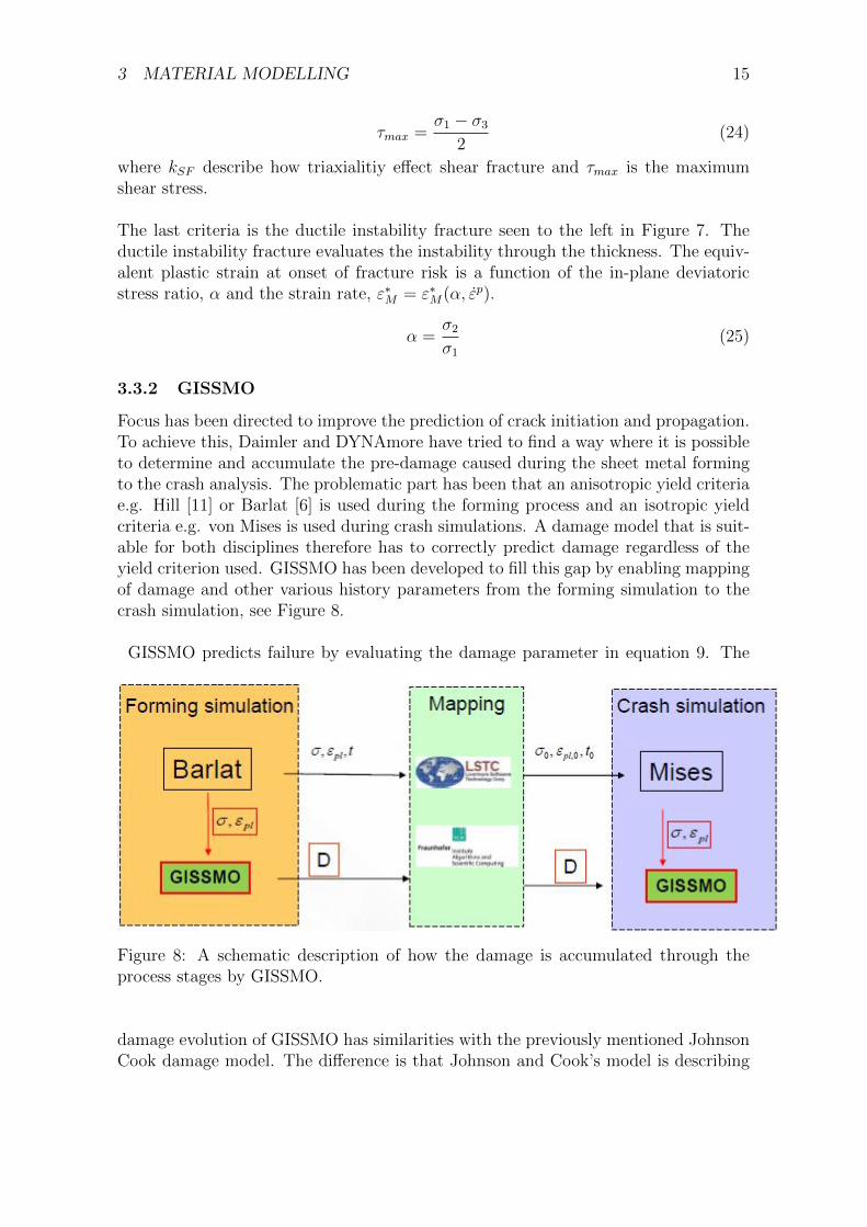
Focus has been directed to improve the prediction of crack initiation and propagation.To achieve this, Daimler and DYNAmore have tried to find a way where it is possibleto determine and accumulate the pre-damage caused during the sheet metal formingto the crash analysis. The problematic part has been that an anisotropic yield criteriae.g. Hill [11] or Barlat [6] is used during the forming process and an isotropic yieldcriteria e.g. von Mises is used during crash simulations. A damage model that is suit-able for both disciplines therefore has to correctly predict damage regardless of theyield criterion used. GISSMO has been developed to fill this gap by enabling mappingof damage and other various history parameters from the forming simulation to thecrash simulation, see Figure 8.

GISSMO predicts failure by evaluating the damage parameter in equation 9. The

Figure 8: A schematic description of how the damage is accumulated through theprocess stages by GISSMO.

damage evolution of GISSMO has similarities with the previously mentioned JohnsonCook damage model. The difference is that Johnson and Cook’s model is describing


the evolution of the damage as a linear expression, but GISSMO describes it as anexponential function

D =n

εfD1− 1

n εp (26)

where D is the current value of the damage, εp is the equivalent plastic strain rate, nis the damage exponent and εf is equivalent plastic stain at failure. If n=1, equation26 is reduced to the Johnson Cook model, see equation 12.

One useful property of GISSMO is to accumulate a measure of instability, F. F evolvesaccording to the following function.

F =n

εcritF 1− 1

n εp (27)

where εcrit is the equivalent plastic strain when instability occur. When F=1, insta-bility is reached and it is now assumed that the damage is coupled to the true stressesthrough

σtrue = σeff [1−(D −Dcrit

1−Dcrit

)m

] (28)

where Dcrit takes the value of the damage parameter when F reaches 1. m is the fadeexponent, which is calibrated to match experiments. If m=1 and Dcrit=0 equation 11is proved to be a generalized expression of equation 26. For further motivation, seereference [7] and [14].

4 RESULTS 17

4 Results

4.1 CrachFEM results

The results presented below are from material test simulations, where CrachFEM hasbeen used as failure criteria. The results are presented for a boron steel, since thecrash simulations that CEVT run often involves failure in this material. Although, itis important to clarify that the working process is suitable for all kind of steels.

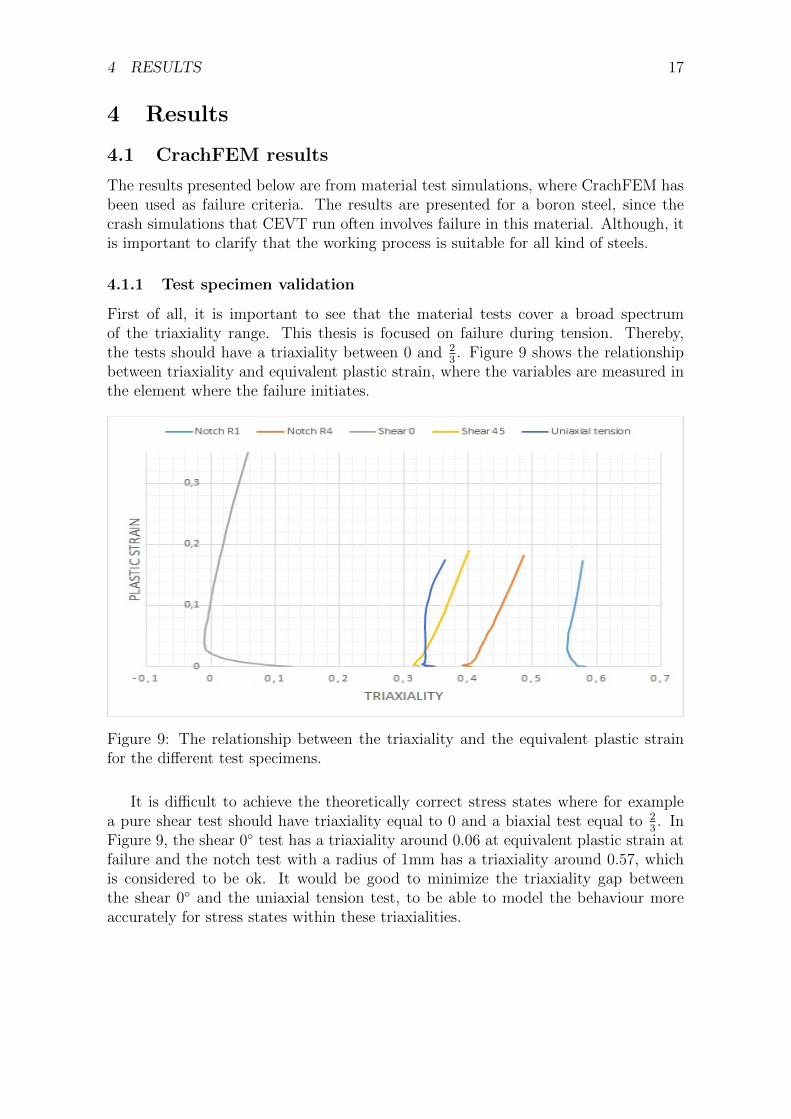
4.1.1 Test specimen validation

First of all, it is important to see that the material tests cover a broad spectrumof the triaxiality range. This thesis is focused on failure during tension. Thereby,the tests should have a triaxiality between 0 and 2

3. Figure 9 shows the relationship

between triaxiality and equivalent plastic strain, where the variables are measured inthe element where the failure initiates.

Figure 9: The relationship between the triaxiality and the equivalent plastic strainfor the different test specimens.

It is difficult to achieve the theoretically correct stress states where for examplea pure shear test should have triaxiality equal to 0 and a biaxial test equal to 2

3. In

Figure 9, the shear 0◦ test has a triaxiality around 0.06 at equivalent plastic strain atfailure and the notch test with a radius of 1mm has a triaxiality around 0.57, whichis considered to be ok. It would be good to minimize the triaxiality gap betweenthe shear 0◦ and the uniaxial tension test, to be able to model the behaviour moreaccurately for stress states within these triaxialities.

4 RESULTS 18

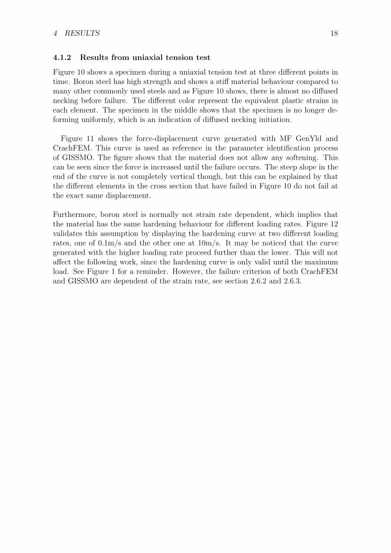
4.1.2 Results from uniaxial tension test

Figure 10 shows a specimen during a uniaxial tension test at three different points intime. Boron steel has high strength and shows a stiff material behaviour compared tomany other commonly used steels and as Figure 10 shows, there is almost no diffusednecking before failure. The different color represent the equivalent plastic strains ineach element. The specimen in the middle shows that the specimen is no longer de-forming uniformly, which is an indication of diffused necking initiation.

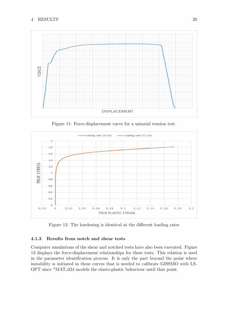
Figure 11 shows the force-displacement curve generated with MF GenYld andCrachFEM. This curve is used as reference in the parameter identification processof GISSMO. The figure shows that the material does not allow any softening. Thiscan be seen since the force is increased until the failure occurs. The steep slope in theend of the curve is not completely vertical though, but this can be explained by thatthe different elements in the cross section that have failed in Figure 10 do not fail atthe exact same displacement.

Furthermore, boron steel is normally not strain rate dependent, which implies thatthe material has the same hardening behaviour for different loading rates. Figure 12validates this assumption by displaying the hardening curve at two different loadingrates, one of 0.1m/s and the other one at 10m/s. It may be noticed that the curvegenerated with the higher loading rate proceed further than the lower. This will notaffect the following work, since the hardening curve is only valid until the maximumload. See Figure 1 for a reminder. However, the failure criterion of both CrachFEMand GISSMO are dependent of the strain rate, see section 2.6.2 and 2.6.3.

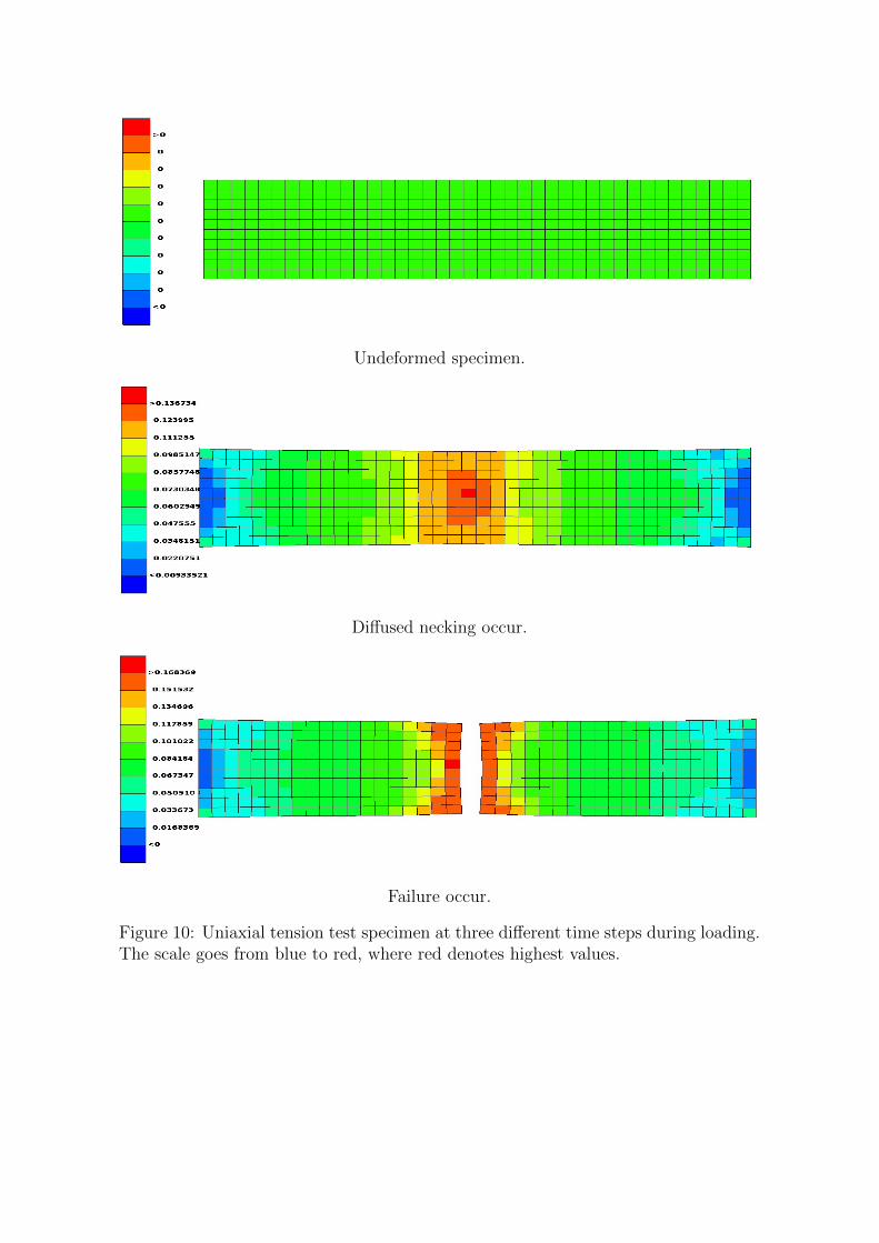
Undeformed specimen.

Diffused necking occur.

Failure occur.

Figure 10: Uniaxial tension test specimen at three different time steps during loading.The scale goes from blue to red, where red denotes highest values.

4 RESULTS 20

Figure 11: Force-displacement curve for a uniaxial tension test.

Figure 12: The hardening is identical at the different loading rates

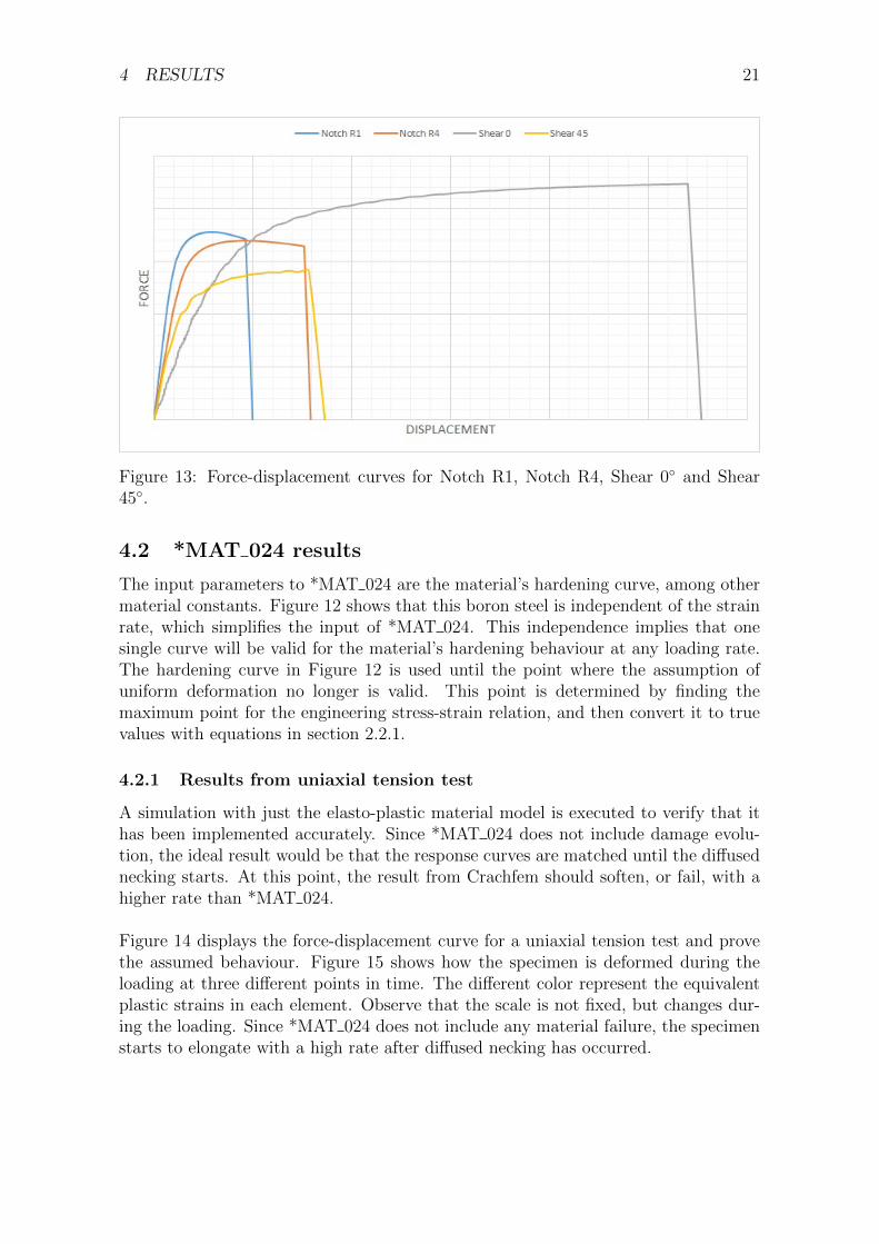
4.1.3 Results from notch and shear tests

Computer simulations of the shear and notched tests have also been executed. Figure13 displays the force-displacement relationships for these tests. This relation is usedin the parameter identification process. It is only the part beyond the point whereinstability is initiated in these curves that is needed to calibrate GISSMO with LS-OPT since *MAT 024 models the elasto-plastic behaviour until that point.

4 RESULTS 21

Figure 13: Force-displacement curves for Notch R1, Notch R4, Shear 0◦ and Shear45◦.

4.2 *MAT 024 results

The input parameters to *MAT 024 are the material’s hardening curve, among othermaterial constants. Figure 12 shows that this boron steel is independent of the strainrate, which simplifies the input of *MAT 024. This independence implies that onesingle curve will be valid for the material’s hardening behaviour at any loading rate.The hardening curve in Figure 12 is used until the point where the assumption ofuniform deformation no longer is valid. This point is determined by finding themaximum point for the engineering stress-strain relation, and then convert it to truevalues with equations in section 2.2.1.

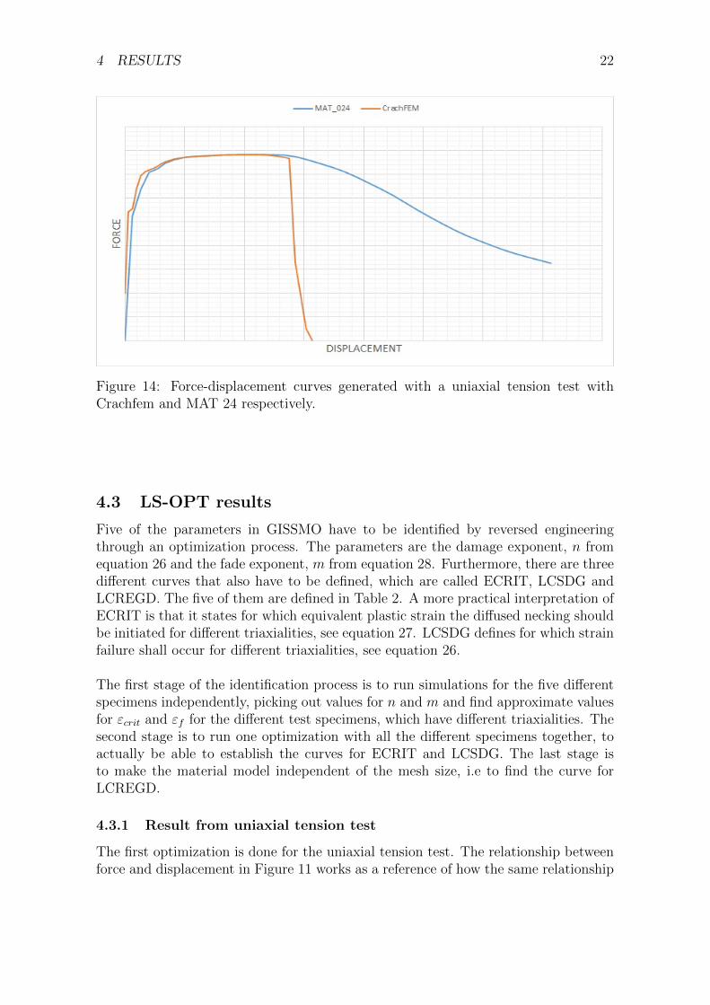
4.2.1 Results from uniaxial tension test

A simulation with just the elasto-plastic material model is executed to verify that ithas been implemented accurately. Since *MAT 024 does not include damage evolu-tion, the ideal result would be that the response curves are matched until the diffusednecking starts. At this point, the result from Crachfem should soften, or fail, with ahigher rate than *MAT 024.

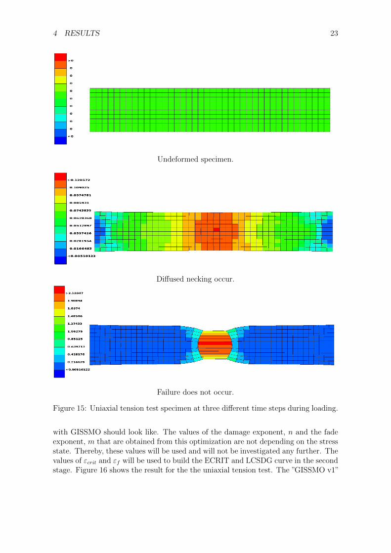
Figure 14 displays the force-displacement curve for a uniaxial tension test and provethe assumed behaviour. Figure 15 shows how the specimen is deformed during theloading at three different points in time. The different color represent the equivalentplastic strains in each element. Observe that the scale is not fixed, but changes dur-ing the loading. Since *MAT 024 does not include any material failure, the specimenstarts to elongate with a high rate after diffused necking has occurred.

4 RESULTS 22

Figure 14: Force-displacement curves generated with a uniaxial tension test withCrachfem and MAT 24 respectively.

4.3 LS-OPT results

Five of the parameters in GISSMO have to be identified by reversed engineeringthrough an optimization process. The parameters are the damage exponent, n fromequation 26 and the fade exponent, m from equation 28. Furthermore, there are threedifferent curves that also have to be defined, which are called ECRIT, LCSDG andLCREGD. The five of them are defined in Table 2. A more practical interpretation ofECRIT is that it states for which equivalent plastic strain the diffused necking shouldbe initiated for different triaxialities, see equation 27. LCSDG defines for which strainfailure shall occur for different triaxialities, see equation 26.

The first stage of the identification process is to run simulations for the five differentspecimens independently, picking out values for n and m and find approximate valuesfor εcrit and εf for the different test specimens, which have different triaxialities. Thesecond stage is to run one optimization with all the different specimens together, toactually be able to establish the curves for ECRIT and LCSDG. The last stage isto make the material model independent of the mesh size, i.e to find the curve forLCREGD.

4.3.1 Result from uniaxial tension test

The first optimization is done for the uniaxial tension test. The relationship betweenforce and displacement in Figure 11 works as a reference of how the same relationship

4 RESULTS 23

Undeformed specimen.

Diffused necking occur.

Failure does not occur.

Figure 15: Uniaxial tension test specimen at three different time steps during loading.

with GISSMO should look like. The values of the damage exponent, n and the fadeexponent, m that are obtained from this optimization are not depending on the stressstate. Thereby, these values will be used and will not be investigated any further. Thevalues of εcrit and εf will be used to build the ECRIT and LCSDG curve in the secondstage. Figure 16 shows the result for the the uniaxial tension test. The ”GISSMO v1”

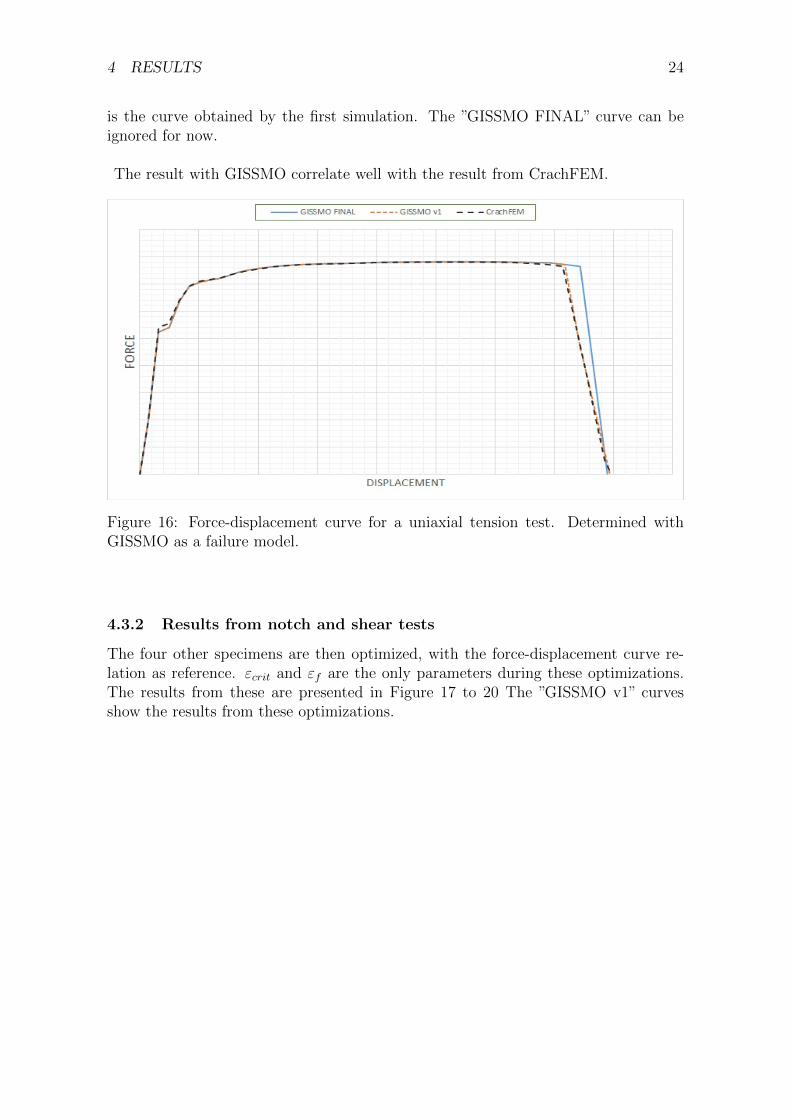
4 RESULTS 24

is the curve obtained by the first simulation. The ”GISSMO FINAL” curve can beignored for now.

The result with GISSMO correlate well with the result from CrachFEM.

Figure 16: Force-displacement curve for a uniaxial tension test. Determined withGISSMO as a failure model.

4.3.2 Results from notch and shear tests

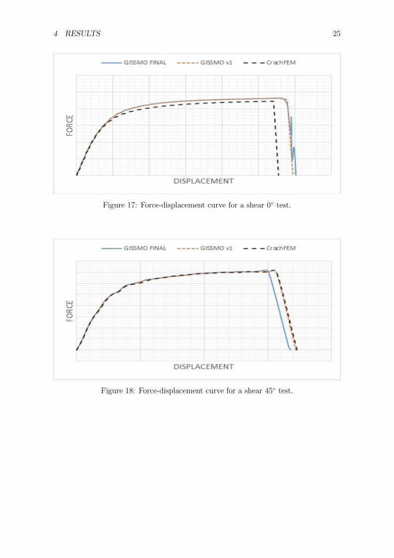
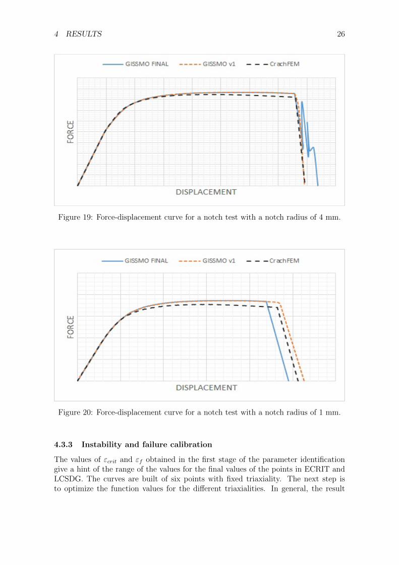
The four other specimens are then optimized, with the force-displacement curve re-lation as reference. εcrit and εf are the only parameters during these optimizations.The results from these are presented in Figure 17 to 20 The ”GISSMO v1” curvesshow the results from these optimizations.

4 RESULTS 25

Figure 17: Force-displacement curve for a shear 0◦ test.

Figure 18: Force-displacement curve for a shear 45◦ test.

4 RESULTS 26

Figure 19: Force-displacement curve for a notch test with a notch radius of 4 mm.

Figure 20: Force-displacement curve for a notch test with a notch radius of 1 mm.

4.3.3 Instability and failure calibration

The values of εcrit and εf obtained in the first stage of the parameter identificationgive a hint of the range of the values for the final values of the points in ECRIT andLCSDG. The curves are built of six points with fixed triaxiality. The next step isto optimize the function values for the different triaxialities. In general, the result

4 RESULTS 27

is changed to the worse during this stage, which is what can be expected since thepoints that form the final ECRIT and LCSDG curves will be influenced by more thanone test at the same time. The resulting curves for ECRIT and LCSDG are shownin Figure 21. It might seem strange that the ECRIT curve takes higher values thanLCSDG at triaxialities between ≈0.35 to ≈0.62. This could be explained since theinstability criterion in equation 27 is not fulfilled before failure i.e. D = 1. Thereare tendencies of this, since the specimen fail without any obvious necking behaviour.”GISSMO FINAL” in Figure 17-20 show the force - displacement relation with thefinal ECRIT and LCSDG curves. The results are generally worse than ”GISSMO v1”,and the results of the notch R4 and the shear 0◦ test in Figure 19 shows an unwantedfailure behaviour due to the disruption in this stage. This disturbance may be dueto the change of stress state of the remaining elements in the critical section whenone of the elements fails. This behaviour disappears if the waist would contain moreelements through its cross section or if the loading rate is reduced.

Figure 21: The relationship between critical plastic strain and triaxiality and therelationship between plastic strain at failure and triaxiality.

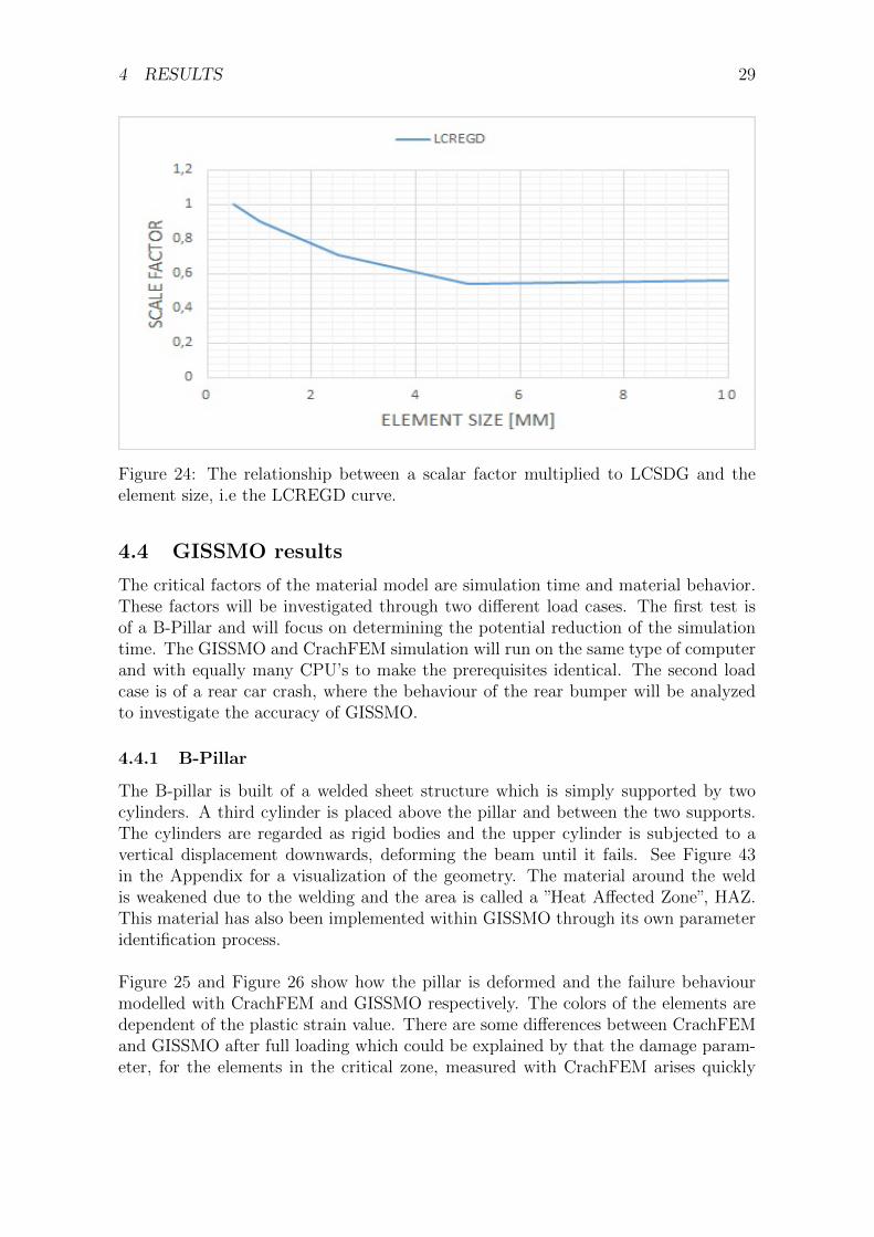
4.3.4 Regularization of element size

The last curve that has to be identified is the LCREGD curve. Figure 22 shows howthe uniaxial tension test modelled with GISSMO is dependent of the element size.The results show that increased element size requires a higher elongation for failure.The identification of LCREGD initiates with the force-displacement curve and sinceno experimental data is available. Effelsberg et al. [7] propose an element size of0.5 mm as reference, trying to make the other curves correlate with this as good aspossible. Figure 23 shows the result and Figure 24 shows the LCREGD curve. Theresult shown in Figure 23 is approved for mesh sizes up to 5 mm. For some reason,

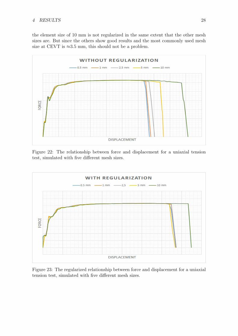
4 RESULTS 28

the element size of 10 mm is not regularized in the same extent that the other meshsizes are. But since the others show good results and the most commonly used meshsize at CEVT is ≈3.5 mm, this should not be a problem.

Figure 22: The relationship between force and displacement for a uniaxial tensiontest, simulated with five different mesh sizes.

Figure 23: The regularized relationship between force and displacement for a uniaxialtension test, simulated with five different mesh sizes.

4 RESULTS 29

Figure 24: The relationship between a scalar factor multiplied to LCSDG and theelement size, i.e the LCREGD curve.

4.4 GISSMO results

The critical factors of the material model are simulation time and material behavior.These factors will be investigated through two different load cases. The first test isof a B-Pillar and will focus on determining the potential reduction of the simulationtime. The GISSMO and CrachFEM simulation will run on the same type of computerand with equally many CPU’s to make the prerequisites identical. The second loadcase is of a rear car crash, where the behaviour of the rear bumper will be analyzedto investigate the accuracy of GISSMO.

4.4.1 B-Pillar

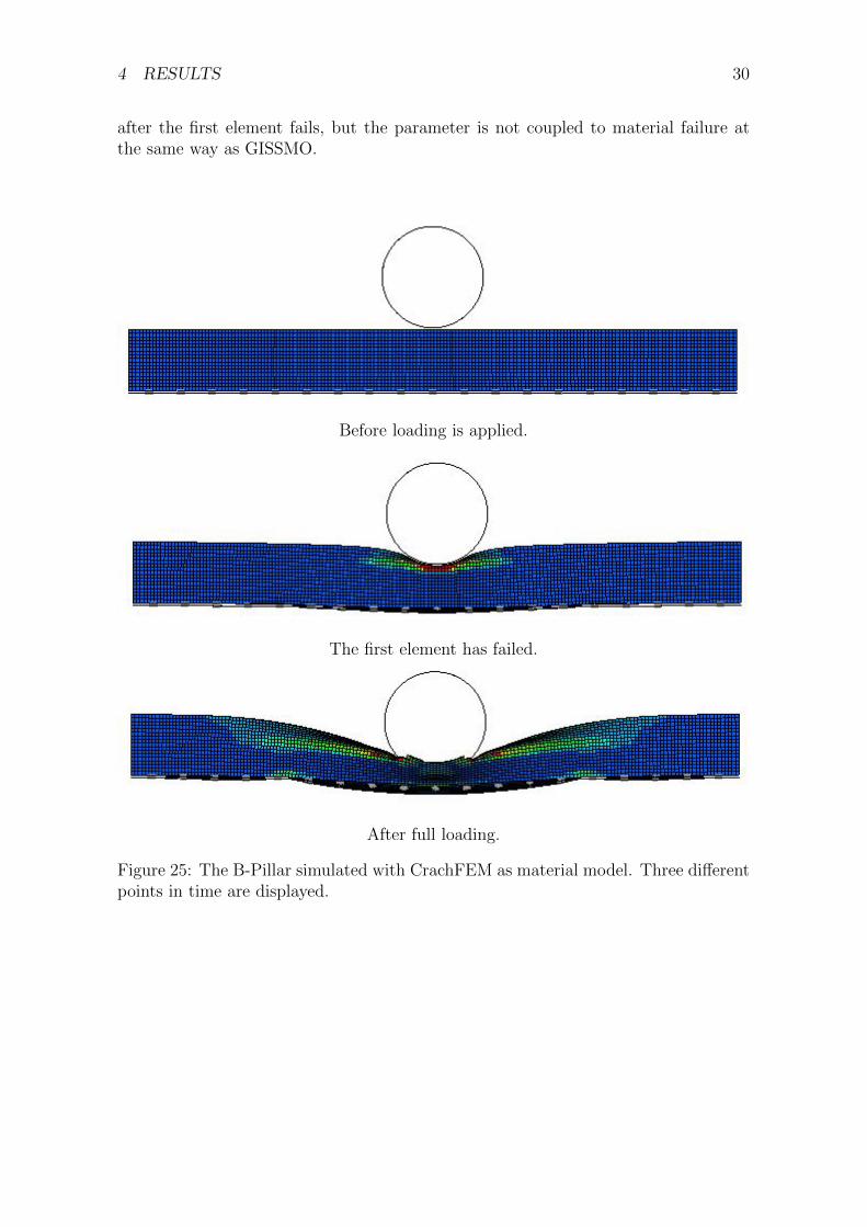
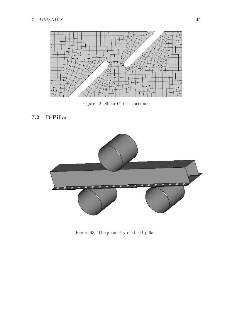
The B-pillar is built of a welded sheet structure which is simply supported by twocylinders. A third cylinder is placed above the pillar and between the two supports.The cylinders are regarded as rigid bodies and the upper cylinder is subjected to avertical displacement downwards, deforming the beam until it fails. See Figure 43in the Appendix for a visualization of the geometry. The material around the weldis weakened due to the welding and the area is called a ”Heat Affected Zone”, HAZ.This material has also been implemented within GISSMO through its own parameteridentification process.

Figure 25 and Figure 26 show how the pillar is deformed and the failure behaviourmodelled with CrachFEM and GISSMO respectively. The colors of the elements aredependent of the plastic strain value. There are some differences between CrachFEMand GISSMO after full loading which could be explained by that the damage param-eter, for the elements in the critical zone, measured with CrachFEM arises quickly

4 RESULTS 30

after the first element fails, but the parameter is not coupled to material failure atthe same way as GISSMO.

Before loading is applied.

The first element has failed.

After full loading.

Figure 25: The B-Pillar simulated with CrachFEM as material model. Three differentpoints in time are displayed.

Before loading is applied.


After full loading.

Figure 26: The B-Pillar simulated with GISSMO as material model. Three differentpoints in time are displayed.

4 RESULTS 32

The results from the B-pillar simulation modelled by the two material models aresimilar. Since CrachFEM work as a failure criteria, the initiation of failure is thefocus. Figure 27 and Figure 28 show the first element that fails for CrachFEM andGISSMO respectively. Since the element that fails first is in the same region and failwithin a short period of time for CrachFEM and GISSMO, the GISSMO is consideredgood enough and will be used for further investigation in the rear crash load case.

Figure 27: First element failed with CrachFEM. The B-pillar is here seen from above.

Figure 28: First element failed with GISSMO. The B-pillar is here seen from above.

4 RESULTS 33

The time has been an key factor for this thesis. For the result to be valid it isimportant that the same CPUs are chosen in the cluster. This is important sincedifferent CPUs can have different quality. The B-pillar simulation took 3 hours, 22minutes and 56 seconds when running with MF GenYld+CrachFEM and 51 min-utes and 52 seconds with *MAT 024 and GISSMO. See Figure 29 and 30 for detailedinformation about the run time. The ”Contact algorithm” and ”Rigid bodies” calcula-tions are specific calculations for the B-Pillar simulation and do not depend on whichmaterial model that is used. Hence, to get a fair comparison of the time reduction,the ”Element processing” stage should be considered instead of ”Total CPU time”.The ”Element processing” takes 180 min 39 s with CrachFEM and 31 min 49.9s withGISSMO. GISSMO results in a time reduction of the ”Element processing” of almost82 percent compared to CrachFEM. Thereby, GISSMO has a huge potential of re-ducing the simulation time, especially when a full car body simulation normally takesabout 14 hours modelled with CrachFEM.

Figure 29: Timing information MY GenYld+CrachFEM, B-pillar.

4 RESULTS 34

Figure 30: Timing information, *MAT 024 and GISSMO, B-pillar.

4.4.2 Rear crash

The final verification of that GISSMO has been implemented correctly is to analyze acomplex load case of a car crash where the rear of the car will be hit by a wagon witha defined velocity. Figure 44 in the Appendix visualize the load case. This test will befocused on what happens with the rear bumper during collision. The first simulationwill model the bumpers behaviour with CrachFEM and the second will model it withGISSMO.

There is a reason why the simulation time is not the focus during this load case.That is because different parts of the car are modelled with different material mod-els. Some of these models do not model material failure since it is not necessary inall areas and it would extend the simulation time further. During this simulation, itis only the material model of the bumper that is changed between the two simulations.

The results will illustrate only the bumper, to make the analysis more clear. Fig-ure 31 and 32 show the deformation of the bumper, from above, at three differentpoints in time. Figure 31 is modelled by CrachFEM and Figure 32 is modelled byGISSMO. The color of the figures represent the equivalent plastic strain.

4 RESULTS 35

Undeformed bumper.


Fully loaded

Figure 31: The deformation of the bumper at three different time steps during loading.Modelled with CrachFEM

4 RESULTS 36

Undeformed bumper.


Fully loaded

Figure 32: The deformation of the bumper at three different time steps during loading.Modelled with GISSMO

The deformations look similar, but a more detailed analysis is needed to evaluatethe result. Figure 33-36 show the bumper, viewed from behind, in its undeformedgeometry to be able to compare the results easier. Figure 33 and 34 show how thelocation of the failure and equivalent plastic strain is varying when the first elementhas failed. Figure 35 and 36 show how the location of the failure and equivalent plasticstrain is varying after full loading. Overall, the results are similar. It is noticed that

4 RESULTS 37

more elements fail using GISSMO than using CrachFEM. Although, the CrachFEMmanual [5] claims that CrachFEM should only be used to determine the initiation ofmaterial failure, which is very similar between GISSMO and CrachFEM.

Figure 33: First element failed. Modelled with CrachFEM.

Figure 34: First element failed. Modelled with GISSMO.

Figure 35: After full loading. Modelled with CrachFEM.

Figure 36: After full loading. Modelled with GISSMO.

5 ANALYSIS 38

5 Analysis

The final comparisons of the material models show similar results. This indicatesthat the parameter identification process works. However, there are some stages thatmay be improved. For example, the triaxiality gap between the shear 0◦ and uniaxialtension test which was previously mentioned, see Figure 9. It may be difficult todesign a test specimen that obtains the wanted triaxiality, but since this thesis is notbased on experimental test results, the material testing does not need to be limitedby standardized test specimens. It is possible to replace the specimens with a loadcase of one element, see Figure 37. All different triaxialities can be generated withthis simple test by changing the displacement controlled loading. This would improvethe process in a couple ways. Partly because of reduced simulation time during thematerial testing and partly because it is possible to direct the stress state in a simpleway. This testing method has been tried, and seems to work well. One problem thatarose with this testing technique is with a pure shear test with a stress state charac-terized by η = 0. Regardless of how long the loading proceeds, the element does notfail. Since the CrachFEM parameters are encrypted, it is difficult to address why thisis the case. It is definitely a testing method that could be further developed.

Figure 37: Load case for one element

5 ANALYSIS 39

One potential with GISSMO is to satisfy the problem that Andrade, Feucht andHaufe [1] highlights, which is the information gap between the stages in the processchain and especially between the forming and crash stage. GISSMO is a model whichcan be used in all product simulations throughout the chain. With GISSMO it ispossible to accumulate and transfer variables between these stages. Hence, a morefaithful result may be achieved from the crash simulation. This has not been the focusduring this thesis, but it is a potential improvement of the material modelling in theautomotive industry.

This thesis has developed a method to implement GISSMO based on computer simu-lations modelled by another material model. One problem that should be flagged foris that there could be some problems by calibrating a material model without accessto any experimental material tests. Even though CrachFEM is based on an extensiveset of material tests, there could still be deviations between a simulated and an ex-perimental result. The deviations may be extended by the gap between GISSMO andCrachFEM, which could make GISSMO come further away from the reality.

6 CONCLUSIONS 40

6 Conclusions

*MAT 024 and GISSMO were implemented to analyze the elasto-plastic and the fail-ure behaviour of a material. The material data for the input parameters were gen-erated from computer simulations using MF GenYld+CrachFEM. *MAT 024 andGISSMO were compared with MF GenYld+CrachFEM during two complex loadcases, one depicting a B-pillar and one depicting a full car body rear crash. Thenew material model has proven to have a potential to reduce the simulation time withalmost 82 percent and has similar material behaviour as the current model. However,one limitation of the result is that *MAT 024 and GISSMO have not been comparedto experimental data.

References

[1] Filipe ANDRADE, Markus FEUCHT, and Andre HAUFE. On the prediction ofmaterial failure in ls-dyna R©: A comparison between gissmo and diem. In 13thInternational LS-DYNA R© Users Conference, 2014.

[2] Donald R Askeland and Pradeep Prabhakar Phule. The science and engineeringof materials. 2003.

[3] Percy Williams Bridgman. Studies in large plastic flow and fracture, volume 177.McGraw-Hill New York, 1952.

[4] Livermore Software Technology Corporation. Ls-opt user’s manual. 2015.

[5] Helmut. Oberhofer Gernot. Dell, Harry. Gese. MF GenYld+CrachFEM 4.2 User’sManual. 2014.

[6] Oana CAZACU Dorel BANABIC, Frederic BARLAT, Dan-Sorin COMSA, Ste-fan WAGNER, and Kurt SIEGERT. Recent anisotropic yield criteria for sheetmetals. 2002.

[7] J Effelsberg, A Haufe, M Feucht, F Neukamm, and P Du Bois. On parameteridentification for the gissmo damage model. In 12th International LS-DYNA R©Users Conference, Dearborn, MI, USA, 2012.

[8] American Society for Testing and Material. Standard Test Methods for TensionTesting of Metallic Materials. 1998.

[9] John O Hallquist et al. Ls-dyna theory manual. Livermore software Technologycorporation, 3, 2006.

[10] Andre Haufe, Paul DuBois, Frieder Neukamm, and Markus Feucht. Gissmo–material modeling with a sophisticated failure criteria. In LS-Dyna DeveloperForum, 2011.

[11] Rodney Hill. A theory of the yielding and plastic flow of anisotropic metals.In Proceedings of the Royal Society of London A: Mathematical, Physical andEngineering Sciences. The Royal Society, 1948.

[12] Jean Lemaitre and Jean-Louis Chaboche. Mechanics of solid materials. Cam-bridge university press, 1994.

[13] Livermore Software Technology Corporation (LSTC). LS-DYNA User’s ManualVolume II, Verision R7.0. 2013.

[14] Frieder Neukamm, Markus Feucht, and Andre Haufe. Considering damage historyin crashworthiness simulations. Ls-Dyna Anwenderforum, 2009.

[15] Niels Saabye Ottosen and Matti Ristinmaa. The mechanics of constitutive mod-eling. Elsevier, 2005.

REFERENCES 42

[16] J R Rice and Dennis Michael Tracey. On the ductile enlargement of voids intriaxial stress fields. Journal of the Mechanics and Physics of Solids, 17(3):201–217, 1969.

[17] BETA CAE Systems SA. Ansa user’s guide. 2015.

[18] Katharina Witowski, Markus Feucht, and Nielen Stander. An effective curvematching metric for parameter identification using partial mapping. In 8th Eu-ropean LS-DYNA, Users Conference Strasbourg, pgs, pages 1–12, 2011.

[19] Liang Xue. Damage accumulation and fracture initiation in uncracked ductilesolids subject to triaxial loading. International Journal of Solids and Structures,44(16):5163–5181, 2007.

[20] Won Y Yang, Wenwu Cao, Tae-Sang Chung, and John Morris. Applied numericalmethods using MATLAB. John Wiley & Sons, 2005.

7 APPENDIX 43

7 Appendix

7.1 Test specimens

Figure 38: Uniaxial tension test specimen

Figure 39: Notch test specimen, radius 4 mm

7 APPENDIX 44

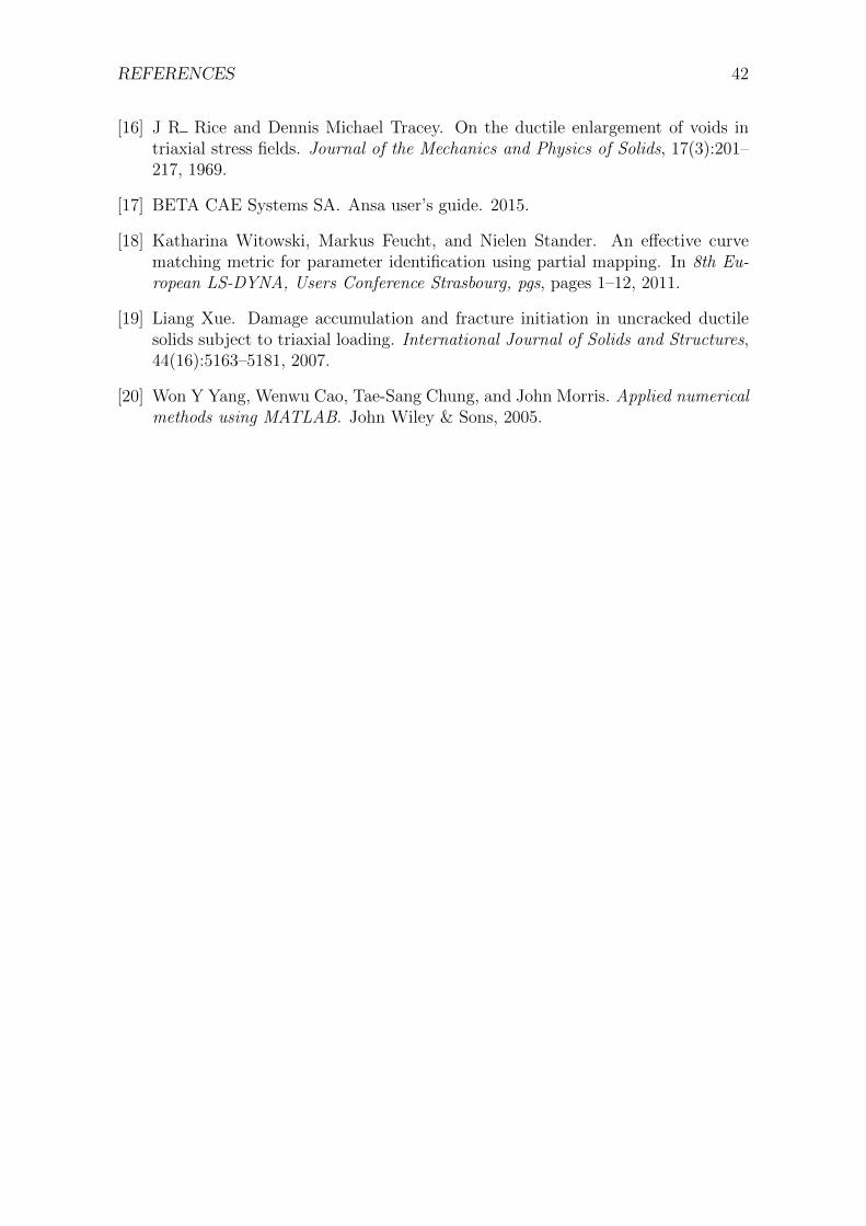
Figure 40: Notch test specimen, radius 1 mm

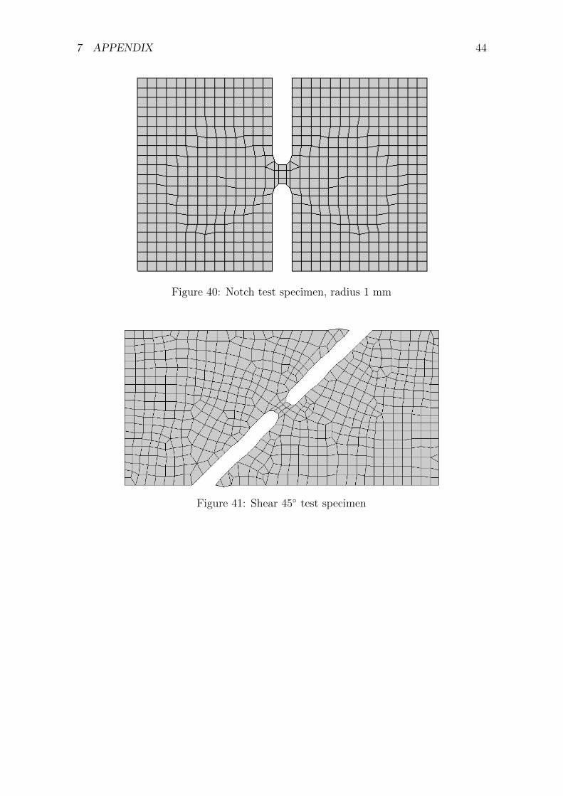
Figure 41: Shear 45◦ test specimen

7 APPENDIX 45

Figure 42: Shear 0◦ test specimen

7.2 B-Pillar

Figure 43: The geometry of the B-pillar.

7 APPENDIX 46

7.3 Rear crash

Figure 44: The geometry of a similar rear crash test.

Evaluation of Material Models to Predict Material Failure ...

Documents