American Journal of Business, Economics and Management 2014; 2(1): 28-40 Published online March 30, 2014 (http://www.openscienceonline.com/journal/ajbem) Evaluation of government income-spending hypothesis nexus in Nigeria: Application of the bound test approach Samson Adeniyi Aladejare Department of Economics, Federal University Wukari, Nigeria Email address [email protected] To cite this article Samson Adeniyi Aladejare. Evaluation of Government Income-Spending Hypothesis Nexus in Nigeria: Application of the Bound Test Approach, American Journal of Business, Economics and Management. Vol. 2, No. 1, 2014, pp. 28-40 Abstract This study is a review of the relationship and dynamic interactions between government revenue and expenditure in Nigeria over the period 1981 to 2012. The analytical technique of Autoregressive Distributed Lag (ARDL) bound test as was exploited. From the results, it is obvious that there is evidence of fiscal synchronization between the fiscal variables. The policy implication of the findings of this study is that government should diversify its sources of revenue. This would ensure moving away from a single product economy to a multi product economy. It is believed if this is done, returns and impact of the non oil sector on government spending and the economy in both the short and long run would be much significant. Furthermore, the government should not make spending-tax decisions in isolation of tax-spend decisions. This is because the joint determination of revenues and expenditures is appealing as long as it effectively restrains the budget deficit. This means that efforts to enrich sources of revenue should be complemented by reductions in spending by Nigeria. Keywords Revenue, Expenditure, Government, Bound Test, Nigeria 1. Introduction Modern governments provide a variety of services through the budget. Such include the provision of economic and social infrastructure, defence, maintenance of law and order, establishment of pension schemes, etc. The extent of government involvment in providing goods and services is subject to spatia-temporal variations. The scope of its functions depends, among other things, on the political and economic orientation of the members of a particular society at a given point in time, as well as their needs and aspirations (Adesola 1995: 13). The performance or discharge of these functions engenders governmental fiscal operations. The fiscal operation of government is basically a concept in duality. On the one hand, the provision of goods and services invariably entails commitment of expenditures. On the other, government has to raise revenues in order to meet its expenditure requirements. Thus, revenue and expenditure describe the gamut of government fiscal operations. However, when fiscal out-turns manifest deficits, public borrowing becomes inevitable. Borrowing, therefore, is a supplementary instrument of government finances. In Nigeria, government expenditures have in the main consistently exceeded government revenues throughout most of the past decades since 1970 except for 1971, 1973- 74, 1979, and 1995-96 periods. The government's purportedly commitment in pursuing rapid economic development programmes as embodied in various developmental plans in Nigeria largely accounts for the fiscal deficits incurred. The expanded role of the public sector resulted in rapid growth of government expenditures. Government budget deficits over the years have not impacted positively on the economy. Such fiscal deficits

Welcome message from author
This document is posted to help you gain knowledge. Please leave a comment to let me know what you think about it! Share it to your friends and learn new things together.
Transcript
American Journal of Business, Economics and Management 2014; 2(1): 28-40
Published online March 30, 2014 (http://www.openscienceonline.com/journal/ajbem)
Evaluation of government income-spending hypothesis nexus in Nigeria: Application of the bound test approach
Samson Adeniyi Aladejare
Department of Economics, Federal University Wukari, Nigeria
Email address
To cite this article Samson Adeniyi Aladejare. Evaluation of Government Income-Spending Hypothesis Nexus in Nigeria: Application of the Bound Test
Approach, American Journal of Business, Economics and Management. Vol. 2, No. 1, 2014, pp. 28-40
Abstract
This study is a review of the relationship and dynamic interactions between government revenue and expenditure in
Nigeria over the period 1981 to 2012. The analytical technique of Autoregressive Distributed Lag (ARDL) bound test as
was exploited. From the results, it is obvious that there is evidence of fiscal synchronization between the fiscal variables.
The policy implication of the findings of this study is that government should diversify its sources of revenue. This
would ensure moving away from a single product economy to a multi product economy. It is believed if this is done,
returns and impact of the non oil sector on government spending and the economy in both the short and long run would
be much significant. Furthermore, the government should not make spending-tax decisions in isolation of tax-spend
decisions. This is because the joint determination of revenues and expenditures is appealing as long as it effectively
restrains the budget deficit. This means that efforts to enrich sources of revenue should be complemented by reductions
in spending by Nigeria.
Keywords
Revenue, Expenditure, Government, Bound Test, Nigeria
1. Introduction
Modern governments provide a variety of services
through the budget. Such include the provision of economic
and social infrastructure, defence, maintenance of law and
order, establishment of pension schemes, etc. The extent of
government involvment in providing goods and services is
subject to spatia-temporal variations. The scope of its
functions depends, among other things, on the political and
economic orientation of the members of a particular society
at a given point in time, as well as their needs and
aspirations (Adesola 1995: 13). The performance or
discharge of these functions engenders governmental fiscal
operations.
The fiscal operation of government is basically a concept
in duality. On the one hand, the provision of goods and
services invariably entails commitment of expenditures. On
the other, government has to raise revenues in order to meet
its expenditure requirements. Thus, revenue and
expenditure describe the gamut of government fiscal
operations. However, when fiscal out-turns manifest
deficits, public borrowing becomes inevitable. Borrowing,
therefore, is a supplementary instrument of government
finances.
In Nigeria, government expenditures have in the main
consistently exceeded government revenues throughout
most of the past decades since 1970 except for 1971, 1973-
74, 1979, and 1995-96 periods. The government's
purportedly commitment in pursuing rapid economic
development programmes as embodied in various
developmental plans in Nigeria largely accounts for the
fiscal deficits incurred. The expanded role of the public
sector resulted in rapid growth of government expenditures.
Government budget deficits over the years have not
impacted positively on the economy. Such fiscal deficits

American Journal of Business, Economics and Management 2014, 2(1): 28-40 29
tend to reduce national savings which invariably affect
economic development. The options available to the
government to stimulate economic growth in this situation
are to reduce government expenditures or raise revenues
through increase in tax. These two options can help to
reduce the budget deficit(s).
Hence, a sound fiscal policy is important to promote
price stability and sustain growth in output and
employment. Fiscal policy is regarded as an instrument that
can be used to lessen short-run fluctuations in output and
employment in many debates of macroeconomic policy. It
can also be used to bring the economy to its potential level.
If policymakers understand the relationship between
government expenditure and government revenue, without
a pause government deficits can be prevented. Hence, the
relationship between government expenditure and
government revenue has attracted significant interest; due
to the fact that the relationship between government
revenue and expenditure has an impact on the budget
deficit. The causal relationship between government
revenue and expenditure has remained an empirically
debatable issue in the field of public finance, (Eita &
Mbazima, 2008). Over the Past three decades, a large
number of studies have investigated the relationship
between government revenue and government expenditure.
This is not surprising given the importance of the subject
matter in public economics; particularly the direction of
causality has important implications for budget deficits.
Thus, understanding the relationship between government
revenue and government expenditure is important from a
policy point of view, especially for a country like Nigeria,
which is suffering from persistent budget deficits.
The focus of this research therefore, is to evaluate the
relationship between federal government revenue
composition and spending composition in Nigeria. To
achieve this broad objective, the long-run relationships and
dynamic interactions between the government revenues and
expenditures in Nigeria over the period 1981-2012 was
examined. This study employed annual data that covers the
period from 1981-2012 for Nigeria. The data were sourced
from the Central Bank of Nigeria Statistical Bulletin
(volume 23) 2012. For the avoidance of doubt, the
variables of interest are government capital expenditure,
government recurrent expenditure, government oil revenue
and non oil revenue revenues.
2. Theoretical and Empirical
Literature Review
2.1. Theories of Expenditure Growth and
Government Revenue
The relationship between government expenditure and
revenue can be categorized under five major hypotheses
which are being examined as follows:
(a) The tax-and-spend hypothesis: The causal
relationship between revenues and government expenditure
is a classic problem of Public Economics. The tax-spend
hypothesis was initially formulated by Friedman (1978)
and Buchanan and Wagner (1978), but these authors
differed in their perspectives. While Friedman argues that
changes in government revenues lead to changes in
government expenditures, thereby having a positive
relationship or direction, Buchanan and Wagner (1978)
postulate that the causal relationship is negative. Friedman
suggests that tax increases will only lead to expenditure
increases resulting in the inability to reduce budget deficits.
In order words; raising taxes will lead to more government
spending and hence to fiscal imbalances. Cutting taxes is,
therefore, the appropriate remedy to budget deficits.
(b) Buchanan and Wagner hypothesis (1978): share the
same view that tax lead government expenditure but that
the direction of causal relationship is negative as earlier
stated. Their point of view is that, with a cut in taxes the
public will perceive that the cost of government programs
has fallen. As a result they will demand more programs
from the government which if undertaken will result in an
increase in government spending. Higher budget deficits
will then be realized since tax revenue will decline and
government spending will increase. Their remedy for
budget deficits is therefore an increase in taxes, (Moalusi,
2004).
(c) Peacock-Wiseman’s Model: The displacement effect
hypothesis expounded by T. Peacock and Jack Wiseman in
their well-known 1961 monograph “The Growth of Public
Expenditure” in the United Kingdom remains one of the
most reliable explanations. According to Peacock and
Wiseman’s hypothesis, government spending tends to
evolve in a step-like pattern, coinciding with social
upheavals, notably wars. This spend-tax hypothesis
suggests that changes in government expenditures lead to
changes in government revenues. Peacock and Wiseman
(1979) argue that temporary increases in government
expenditures due to “crises” can lead to permanent
increases in government revenues often called the
“displacement effect”.
(d) The Fiscal Synchronization hypothesis: The third
hypothesis known as fiscal synchronization suggests
bidirectional causation between revenues and spending
(Musgrave, 1966; Meltzer and Richard, 1981). The fiscal
synchronization hypothesis which was suggested by
Meltzer and Richard (1981), asserts that there is a feedback
relationship between revenue and expenditure and both
interact interdependently. It postulates that governments
take decisions about revenues and expenditures
simultaneously by analyzing costs and benefits of
alternative programs. Therefore, this view precludes
unidirectional causation from revenue to spending or from
spending to revenue.
(e) The fiscal neutrality school: Proposed by Baghestani
and McNown (1994) believe that none of the above
hypotheses describes the relationship between government
revenues and expenditure. Government expenditure and
revenues are each determined by the long run economic
30 Samson Adeniyi Aladejare: Evaluation of Government Income-Spending Hypothesis Nexus in Nigeria: Application of the
Bound Test Approach
growth reflecting the institutional separation between
government revenues and expenditure that infers that
revenue decisions are made independent so as expenditure
decisions.
2.2. Empirical Literature Review
Considerable empirical works have been done using
different econometric methods, studies have reached
different results. Different studies have focused on different
countries, time periods, and have used different proxy
variables for government revenue and expenditure.
Tan Juat Hong (2009), investigates the causal
relationships between government spending and revenue
for Malaysia. The study uses annual data, a Johansen
cointegration test and an error-correction model. A
preliminary test shows that government revenue and
expenditure are cointegrated. While empirical results
support the spend-and-tax hypothesis for Malaysia. Thus,
concluding that fiscal policy may not be effective enough
to curb the rising budget deficits over the long term and
may even reduce private saving and investment. Extensive
expenditure reforms through fiscal synchronisation were
suggested.
Yaya Keho (2009), uses annual data for the period of
1960 - 2005 to investigate the causal relationship between
government revenues and spending in Côte d’Ivoire and
adopting a cointegration test analysis. The empirical
findings reveal a positive long-run unidirectional causality
running from revenues to expenditures.
Zapf and Payne (2009), evaluated the long-run
association between aggregate state and local government
revenue and expenditures in the case of US by using Engle
Granger cointegration test associated with the Threshold
Autoregressive (TAR) and Momentum Threshold
Autoregressive (MTAR) cointegration techniques and error
correction model (ECM). They indicated that state and
local government expenditures reflect the budget
disequilibrium in the long run, while in the short run; state
and local government expenditures have a significant effect
on the state and local government revenues.
Gil-Alana (2009), examined the association between the
US government expenditures and revenues applying
fractional cointegration and ECM techniques. His result
found no evidence of cointegration at any degree while at a
structural break in 1973 fractional cointegration is found.
Hong (2009), for Malaysia, uses a Johansen
cointegration test and an error-correction model for
causality and annual data over the period 1970 to 2007. His
results show that government revenue and expenditure are
cointegrated and the spend-and-tax hypothesis is confirmed.
Chaudhuri and Sengupta (2009), by using an error-
correction model and Granger causality test for southern
states in India reported that the tax-spend hypothesis is
supported by the analysis and also the spend-tax hypothesis
is valid for some states.
Ho and Huang (2009), tested the hypothesis of tax-spend,
spend-tax, or fiscal synchronization applies to the 31
Chinese provinces using panel data covering 1999 to 2005.
Their results based on multivariate panel error correction
models show that there is no significant causality between
revenues and expenditures in the short run. However, in the
long-run, bidirectional causality exists between revenues
and expenditures, thus supporting the fiscal
synchronization hypothesis for Chinese provinces over this
sample period. Recently for developed country,
Afonso and Rault (2009), investigated causality between
government spending and revenue in the EU by adopting
new econometric technical bootstrap panel analysis in the
period 1960-2006. Spend and-tax causality is found for
Italy, France, Spain, Greece, and Portugal, while tax-and-
spend evidence is present for Germany, Belgium, Austria,
Finland and the UK, and for several EU New Member
States.
Chang and Chiang (2009) consider a sample of 15
OECD countries test for the long-run relationship between
government revenues and government expenditures over
the period 1992-2006. They find evidence of bidirectional
causality between government revenues and expenditures,
supporting the fiscal synchronization hypothesis by using
panel cointegration, and panel Granger causality test
techniques.
Stallmann and Deller (2010), analyzed the impact of
constitutional Tax and Expenditure Limits (TELs) on
growth rates of convergence using a panel techniques in a
case of US data from 1987 to 2004, suggested that state
revenue and expenditure limits have negatively affected
income growth and slowed down convergence.
Khalid .I. Bataineh (2010), examined the causal
relationship between government revenues and
expenditures of the Jordan government over the period
from 1980 to 2008 using cointegration and error-correction
methodology. The empirical results showed a unidirectional
causality running from expenditures to revenues (spend–
revenue hypothesis), suggesting the preference of
controlling or reducing expenditures.
Mohsen Mehrara et al. (2011), Investigate the
relationship between government revenue and government
expenditure in 40 Asian countries for the period of 1995 to
2008. A cointegration relationship between government
revenue and government expenditure by applying Kao
panel cointegration test was adopted. The causality tests
indicate that there is a bidirectional causal relationship
between government expenditure and revenues in both the
long and the short run confirming fiscal synchronization
hypothesis.
Omo Aregbeyen and Taofik Mohammed (2012),
examines the long-run relationships and dynamic
interactions between the government revenues and
expenditures in Nigeria over the period 1970 to 2008. And
adopting the technique of Autoregressive Distributed Lag
(ARDL) bound test in their study. From their results, it was
evident that there is the existence of a long run relationship
between government expenditures and revenues when
government expenditure is made the dependent variable.
American Journal of Business, Economics and Management 2014, 2(1): 28-40 31
However, when revenue was made the dependent variable,
no evidence of a long run relationship was found. The tax-
spend hypothesis was therefore confirmed. Attributing this
perhaps, to oil revenue dominance in Nigeria’s government
revenue profile and fiscal operations over time.
Emelogu C. Obioma, and Uche M. Ozughalu (2012),
empirically analyzed the relationship between government
revenue and government expenditure in Nigeria, using time
series data from 1970 to 2007, obtained from the Central
Bank of Nigeria (2004, 2007). They employed the Engel-
Granger two-step cointegration technique, the Johansen
cointegration method and the Granger causality test within
the Error Correction Modeling (ECM) framework.
Empirical findings from the study indicate, among other
things, that there is a long-run relationship between
government revenue and government expenditure in
Nigeria. There is also evidence of a unidirectional causality
from government revenue to government expenditure. Thus,
the findings support the revenue spend hypothesis for
Nigeria, indicating that changes in government revenue
induce changes in government expenditure.
Samson A. A. and Ani E.C. (2012), examined the
structure of federal government revenue and expenditure in
Nigeria, from 1961-2010. Using Granger causality test
through cointegrated vector autoregression (VAR) methods;
their result shows that there is a bi-directional causality
between government revenue and government expenditure.
The outcome of the bi-directional causality between
government revenue and expenditure supports the fiscal
synchronization hypothesis. They therefore, suggest that
the federal government should not make spending-tax
decisions in isolation of tax-spend decisions. This is
because the joint determination of revenues and
expenditures is appealing as long as it effectively restrains
the budget deficit. They therefore recommend that efforts at
enhancing sources of revenue should be accompanied by
reductions in government spending for Nigeria.
3. Methodology and Estimation
Technique
The study method adopted in this work is the new Auto-
Regressive Distributed Lag (ARDL) bounds testing
approach developed by Pesaran et al. (2001). The
justification for the selection of this approach is base on the
advantages of the ARDL for testing the existence of a
cointegrating relationship either in the short-run or long-run.
Pesaran et al. (2001) developed a new Auto-Regressive
Distributed Lag (ARDL) bounds testing approach for
testing the existence of a cointegration relationship.
The bound testing approach has certain econometric
advantages in comparison to other single cointegration
procedures (Engle and Granger, 1987; Johansen, 1988).
Firstly, endogeneity problems and inability to test
hypotheses on the estimated coefficients in the long-run
associated with the Engle-Granger (1987) method are
avoided. Secondly, the long and short-run parameters of the
model in question are estimated simultaneously. Thirdly,
the econometric methodology is relieved of the burden of
establishing the order of integration amongst the variables
and of pre-testing for unit roots. The ARDL approach to
testing for the existence of a long-run relationship between
the variables in levels is applicable irrespective of whether
the underlying regressors are purely I(0), purely I(1), or
fractionally integrated. Finally, as put forward in Narayan
(2005), the small sample properties of the bounds testing
approach are believed to be superior to that of multivariate
cointegration. The approach, therefore, is a modification of
the Auto-Regressive Distributed Lag (ARDL) framework
while overcoming the inadequacies associated with the
presence of a mixture of I(0) and I(1) regressors in a
Johansen-type framework.
3.1. Data Descriptions
In this study, GREXP is defined as Government
Recurrent Expenditure: this can be referred to as the
running cost the government incurs every year. They
include expenses on defence and internal security,
education, health, transfers, communication, etc. GCEXP is
Government Capital Expenditure; this includes expenses
such as: construction of roads, bridges, power plants,
houses, etc. NOREV is Non OIL revenue the government
makes from sectors other than oil such as: agriculture,
mining, tourism, manufacturing, etc. OREV is the Oil
Revenue accruing annually to the government every year. It
encompasses all revenue the government makes from the
mining of crude oil by its agencies and multinational
corporations and private indigenous investors in the oil
sector. Such of the revenue are in form of royalties and
licences fees on the exploration of crude oil. The annual
time series data used is sourced from the Central Bank of
Nigeria Statistical Bulletin volume 23, December 2012 and
covers the period from 1981 to 2012.
3.2. Estimation Technique
To obtain healthy results, we utilize the ARDL approach
to determine the existence of long and short-run
relationships. ARDL is extremely useful because it allow us
to analyze the presence of equilibrium in terms of long-run
and short-run dynamics without losing long-run
information. Following the literature review above, the
relationship between government spending and revenue can
be expressed in four functional forms as shown below. The
rationale is to show how the various disaggregated
components of revenue and expenditure are interrelated.
Thus, there are four possible functional forms which are
expressed as:
GREXP = f (GCEXP, NOREV, OREV ) (1)
GCEXP = f (GREXP, NOREV, OREV ) (2)
NOREV= f (GREXP, GCEXP, OREV) (3)
32 Samson Adeniyi Aladejare: Evaluation of Government Income-Spending Hypothesis Nexus in Nigeria: Application of the
Bound Test Approach
OREV = f (GREXP, GCEXP, NOREV) (4)
Where:
GREXP = Government Recurrent Expenditure
GCEXP = Government Capital Expenditure
NOREV = Non Oil Revenue
OREV = Oil Revenue
To empirically analyze the above functional forms, the
ARDL model specification is used to show the long-run
relationships and dynamic interactions between
government spending and government expenditure using
Autoregressive Distributed Lag (ARDL) co-integration test
popularly known as the bound test. This method is adopted
for this study for three reasons. Firstly, compare to other
multivariate co-integration methods, the bounds test is a
simple technique because it allows the co-integration
relationship to be estimated by OLS once the lag order of
the model is identified. Secondly, adopting the bound
testing approach means that pretest such as unit root test is
not required. This implies that the regressors can be either
I(0), purely I(1) or mutually co-integrated. Thirdly, the
long-run and short run parameters of the models can be
simultaneously estimated. The procedure will however
crash in the presence of I(2) series.
This study apply the bounds test procedure by modelling
the long-run equation first as a general vector
autoregressive (VAR) model of order p, in zt :
(1)
Where:
µ0 = vector of intercepts
The corresponding Vector Error Correction Model
(VECM) for Eq. (1) is derived as:
(2)
Where; ∆ represent the first difference operator, γ and λ
represents vector matrices that contain the long-run
multipliers and short-run dynamic coefficients of the
VECM respectively. Zt is a vector of Xt and Yt variables
respectively. Yt (GREXPt, GCEXPt, NOREVt, OREVt,) is
the regressand and Xt (GREXPt, GCEXPt, NOREVt, OREVt,)
is a vector matrix of a set of regressors. As a condition, Yt
must be an I(1) variable, while Xt regressors can either be
I(0) and I(1). εt is a stochastic error term. Assuming
unrestricted intercepts and no trends, Eq. (2) becomes an
unrestricted error correction model (UECM) as:
(3)
Incorporating the variables of interest, the UECM of Eq.
3 becomes:
(4)
(5)
(6)
(7)
Where:
β = long run coefficients
λ = short run coefficients
p = lag length for the Unrestricted Error-Correction
Model (UECM)
∆ = first differencing operator
q, u, v, w = white noise disturbance error term.
3.3. ARDL Testing Approach
The testing procedure of the ARDL bounds test is
performed in three steps. First, OLS is applied to Eq. (4, 5,
6 and 7) to test for the existence of a cointegrating long-run
relationship normalized on the regressands based on the
Wald test (F-statistics) for the joint significance of the
lagged levels of the variables (i.e., H0: B1 = B2 = B3 = B4 =
B5 = 0) as against the alternative (H1:B1≠ B2≠ B3≠ B4≠
American Journal of Business, Economics and Management 2014, 2(1): 28-40 33
B5≠ 0). The computed F-statistic is then compared with the
non-standard critical bounds values as reported in Pesaran
et al. (2001). The lower and upper bounds critical values
assumes that the regressors are purely I(0), purely I(1),
respectively. If the F-statistic is above the upper critical
value, the null hypothesis of no long-run relationship can
be rejected irrespective of the orders of integration for the
time series. Conversely, if the test statistic falls below the
lower critical value the null hypothesis cannot be rejected.
Finally, if the statistic falls between the lower and upper
critical values, the result is inconclusive. Once
cointegration is established, the second step involves
estimating the long-run ARDL model for equations 4, 5, 6
and 7 respectively:
(8)
(9)
(10)
(11)
The final step involves estimating an Error Correction
Model (ECM) as derived from Eqs. 8, 9, 10 and 11
respectively to obtain the short-run dynamic parameters as
specified below:
(12)
(13)
(14)
(15)
Where:
ecmt-1 = the error correction mechanism lagged for one
period
δ = the coefficients for measuring speed of adjustment
4. Empirical Results
4.1. Unit Roots Tests
Before proceeding with the ARDL bounds test, the
stationarity status of all variables to determine their order
of integration is carried out. This is to ensure that the
variables are not I(2) stationary so as to avoid spurious
results. In the presence of I(2) variables the computed F-
statistics provided by Pesaran et al. (2001) are not valid
because the bounds test is based on the assumption that the
variables are I(0) or I(1). Therefore, the implementation of
unit root tests in the ARDL procedure might still be
necessary in order to ensure that none of the variables is
integrated of order 2 or beyond.
This study applied a more efficient univariate DF-GLS
test for autoregressive unit root recommended by Elliot,
Rothenberg, and Stock (ERS, 1996). The test is a simple
modification of the conventional Augmented Dickey-Fuller
(ADF) t-test as it applies generalized least squares (GLS)
de-trending prior to running the ADF test regression.
Compared with the ADF tests, the DF-GLS test has the best
overall performance in terms of sample size and power. It
“has substantially improved power when an unknown mean
or trend is present” (ERS, p.813). The test regression
included both a constant with no trend and a constant with
trend for the first differences of the variables as all the
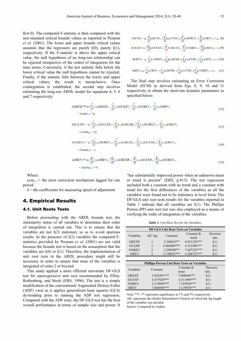
variables were found not to be stationary at level form. The
DF-GLS unit root tests results for the variables reported in
Table 1 indicate that all variables are I(1). The Phillips
Perron (PP) unit root test was also employed as a means of
verifying the order of integration of the variables.
Table 1. Unit Root Test for the Variables.
DF-GLS Unit Root Tests on Variables
Variables AIC lag Constant Constant &
trend
Decision
rule
GREXP 1 2.384652** 6.921236*** I(1)
GCEXP 2 6.468409*** 6.721496*** I(1)
NOREV 2 2.289389** 7.447325*** I(1)
OREV 2 5.150035*** 6.288725*** I(1)
Phillips-Perron Unit Root Tests on Variables
Variables Constant Constant &
trend
Decision
rule
GREXP 5.026381*** 7.088044*** I(1)
GCEXP 6.477828*** 6.511896*** I(1)
NOREV 5.372030*** 7.255956*** I(1)
OREV 7.068894*** 11.39974*** I(1)
Note: ***, ** represents significance at 1% and 5% respectively.
AIC represents the Akaike Information Criterion on which the lag length
of the variables was decided
Source: Computed by Author
34 Samson Adeniyi Aladejare: Evaluation of Government Income-Spending Hypothesis Nexus in Nigeria: Application of the
Bound Test Approach
The result in table 1 shows that the variables are stationary
at 1st differencing. Therefore we reject the null hypothesis of
a unit root for the variables and accept the alternative of no
unit root process with the variables. Thus, concluding that
the variables are stationary at their 1st difference.
4.2. Bounds Tests for Cointegration
In the first step of the ARDL testing procedure, Eq.4, 5,
6 and 7 were tested respectively for a cointegrating long-
run analysis with normalization on the dependent variables.
To select the appropriate lag length for the first differenced
variables, we adopted a general-to-specific approach using
an unrestricted VAR by means of Akaike Information
Criterion (AIC). For brevity, the results of the lag selection
are not reported; however, a maximum of 3 lags was used.
As argued by Pesaran and Pesaran (1997), variables ‘in first
difference are of no direct interest’ to the bounds
cointegration test. Hence, any result that supports
cointegration in at least one lag structure provides evidence
for the existence of a long-run relationship. The F-statistic
tests the joint null hypothesis that the coefficients of the
lagged level variables are zero (i.e. no long-run relationship
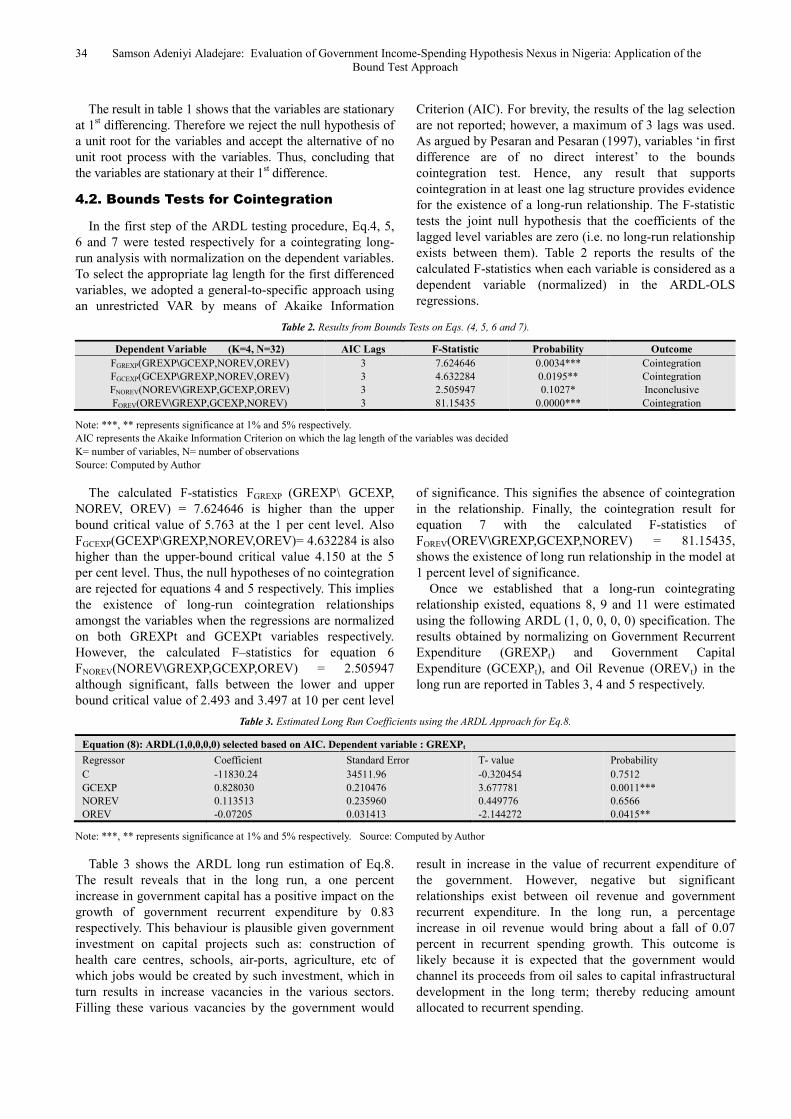
exists between them). Table 2 reports the results of the
calculated F-statistics when each variable is considered as a
dependent variable (normalized) in the ARDL-OLS
regressions.
Table 2. Results from Bounds Tests on Eqs. (4, 5, 6 and 7).
Dependent Variable (K=4, N=32) AIC Lags F-Statistic Probability Outcome
FGREXP(GREXP\GCEXP,NOREV,OREV)
FGCEXP(GCEXP\GREXP,NOREV,OREV)
FNOREV(NOREV\GREXP,GCEXP,OREV)
FOREV(OREV\GREXP,GCEXP,NOREV)
3
3
3
3
7.624646
4.632284
2.505947
81.15435
0.0034***
0.0195**
0.1027*
0.0000***
Cointegration
Cointegration
Inconclusive
Cointegration
Note: ***, ** represents significance at 1% and 5% respectively.
AIC represents the Akaike Information Criterion on which the lag length of the variables was decided
K= number of variables, N= number of observations
Source: Computed by Author
The calculated F-statistics FGREXP (GREXP\ GCEXP,
NOREV, OREV) = 7.624646 is higher than the upper
bound critical value of 5.763 at the 1 per cent level. Also
FGCEXP(GCEXP\GREXP,NOREV,OREV)= 4.632284 is also
higher than the upper-bound critical value 4.150 at the 5
per cent level. Thus, the null hypotheses of no cointegration
are rejected for equations 4 and 5 respectively. This implies
the existence of long-run cointegration relationships
amongst the variables when the regressions are normalized
on both GREXPt and GCEXPt variables respectively.
However, the calculated F–statistics for equation 6
FNOREV(NOREV\GREXP,GCEXP,OREV) = 2.505947
although significant, falls between the lower and upper
bound critical value of 2.493 and 3.497 at 10 per cent level
of significance. This signifies the absence of cointegration
in the relationship. Finally, the cointegration result for
equation 7 with the calculated F-statistics of
FOREV(OREV\GREXP,GCEXP,NOREV) = 81.15435,
shows the existence of long run relationship in the model at
1 percent level of significance.
Once we established that a long-run cointegrating
relationship existed, equations 8, 9 and 11 were estimated
using the following ARDL (1, 0, 0, 0, 0) specification. The
results obtained by normalizing on Government Recurrent
Expenditure (GREXPt) and Government Capital
Expenditure (GCEXPt), and Oil Revenue (OREVt) in the
long run are reported in Tables 3, 4 and 5 respectively.
Table 3. Estimated Long Run Coefficients using the ARDL Approach for Eq.8.
Equation (8): ARDL(1,0,0,0,0) selected based on AIC. Dependent variable : GREXPt
Regressor Coefficient Standard Error T- value Probability
C
GCEXP
NOREV
OREV
-11830.24
0.828030
0.113513
-0.07205
34511.96
0.210476
0.235960
0.031413
-0.320454
3.677781
0.449776
-2.144272
0.7512
0.0011***
0.6566
0.0415**
Note: ***, ** represents significance at 1% and 5% respectively. Source: Computed by Author
Table 3 shows the ARDL long run estimation of Eq.8.
The result reveals that in the long run, a one percent
increase in government capital has a positive impact on the
growth of government recurrent expenditure by 0.83
respectively. This behaviour is plausible given government
investment on capital projects such as: construction of
health care centres, schools, air-ports, agriculture, etc of
which jobs would be created by such investment, which in
turn results in increase vacancies in the various sectors.
Filling these various vacancies by the government would
result in increase in the value of recurrent expenditure of
the government. However, negative but significant
relationships exist between oil revenue and government
recurrent expenditure. In the long run, a percentage
increase in oil revenue would bring about a fall of 0.07
percent in recurrent spending growth. This outcome is
likely because it is expected that the government would
channel its proceeds from oil sales to capital infrastructural
development in the long term; thereby reducing amount
allocated to recurrent spending.
American Journal of Business, Economics and Management 2014, 2(1): 28-40 35
Table 4. Estimated Long Run Coefficients using the ARDL Approach for Eq.9.
Equation (8): ARDL(1,0,0,0,0) selected based on AIC. Dependent variable : GCEXPt
Regressor Coefficient Standard Error T- value Probability
C
GREXP
NOREV
OREV
29430.68
0.040066
-0.28649
0.072373
23400.58
0.142712
0.159991
0.021299
1.176372
6.554069
-1.674885
3.178289
0.2501
0.0000***
0.1059
0.0038***
Note: *** represents significance at 1%. Source: Computed by Author
Table 4 above is an outcome of the estimated ARDL long
run relationship for equation 9. The result shows that in the
long run capital outlay respond positively to growth in
recurrent outlays of the government as well as growth in oil
revenues respectively. The result shows that in the long run,
government capital expenditure would rise by 0.04 percent
to a one percent increase in recurrent outlay growth. This is
plausible in the sense that government investment on
human capital can have a long term effect on improved and
quality productivity of labour. Thus, making the
government less dependent on foreign labour for high
skilled technical duties. Similarly, capital spending would
grow by 0.07 percent with a 1 percent increase in oil
revenue. This is also likely given that capital expenditure in
Nigeria depends almost entirely on proceeds from oil
revenue of the government.
Table 5. Estimated Long Run Coefficients using the ARDL Approach for Eq.11.
Equation (8): ARDL(1,0,0,0,0) selected based on AIC. Dependent variable : OREVt Regressor Coefficient Standard Error T- value Probability C GREXP GCEXP NOREV
1340541.49 22.0366 1.3258 -7.5961
218436.8 1.064582 1.332168 1.493467
0.823496 2.777613 0.133547 -0.682497
0.4177 0.0100*** 0.8948 0.5010
Note: *** represents significance at 1%. Source: Computed by Author
Table 5 is a long run estimation of model 11 which
shows only recurrent expenditure being the sole fiscal
variable in the long run to impact on oil revenue of the
government. The result shows that a percentage increase in
recurrent spending would result in oil revenue growing by
22 percent. This result means that government expenditure
on human capital development, through various funding
agencies such as: the Tertiary Education Trust Fund
(TETfund), Nigerian National Petroleum Company
(NNPC), Petroleum Tertiary Development Fund (PTDF),
etc would reduce the sector’s reliance on foreign high
skilled labour. Thereby, increasing the oil revenue earnings
to the government.
Following the determination of the long run relationships
between the variables above, the short run results for
equations 12, 13 and 14 are presented below respectively.
The study found no existing short run relationship in
equation 15. This therefore means that oil revenue growth
is a long run phenomenon rather than short run.
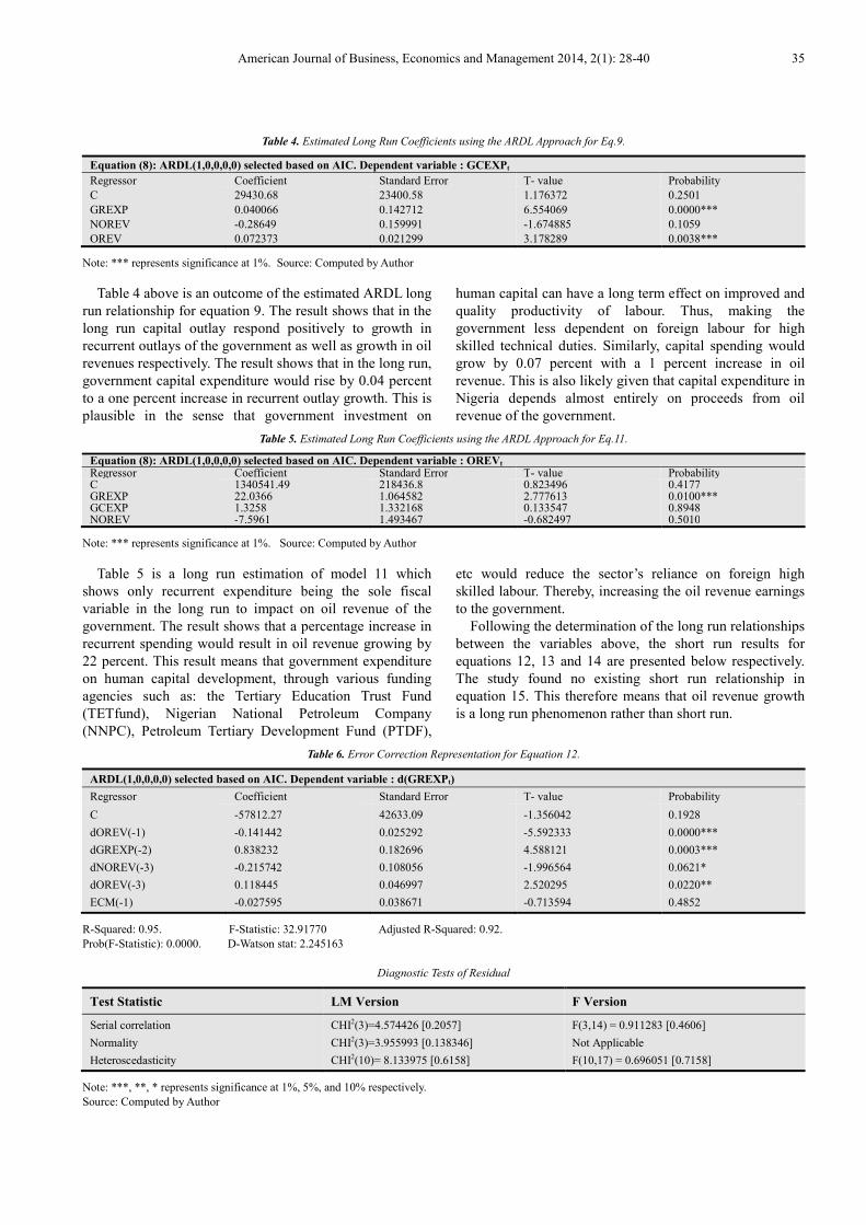
Table 6. Error Correction Representation for Equation 12.
ARDL(1,0,0,0,0) selected based on AIC. Dependent variable : d(GREXPt)
Regressor Coefficient Standard Error T- value Probability
C
dOREV(-1)
dGREXP(-2)
dNOREV(-3)
dOREV(-3)
ECM(-1)
-57812.27
-0.141442
0.838232
-0.215742
0.118445
-0.027595
42633.09
0.025292
0.182696
0.108056
0.046997
0.038671
-1.356042
-5.592333
4.588121
-1.996564
2.520295
-0.713594
0.1928
0.0000***
0.0003***
0.0621*
0.0220**
0.4852
R-Squared: 0.95. F-Statistic: 32.91770 Adjusted R-Squared: 0.92.
Prob(F-Statistic): 0.0000. D-Watson stat: 2.245163
Diagnostic Tests of Residual
Test Statistic LM Version F Version
Serial correlation
Normality
Heteroscedasticity
CHI2(3)=4.574426 [0.2057]
CHI2(3)=3.955993 [0.138346]
CHI2(10)= 8.133975 [0.6158]
F(3,14) = 0.911283 [0.4606]
Not Applicable
F(10,17) = 0.696051 [0.7158]
Note: ***, **, * represents significance at 1%, 5%, and 10% respectively.
Source: Computed by Author
36 Samson Adeniyi Aladejare: Evaluation of Government Income-Spending Hypothesis Nexus in Nigeria: Application of the
Bound Test Approach
Table 6 gives the short run relationship captured by
equation 12. From the estimated result presented above, an
interesting find is the inverse relationship between oil
proceeds and government recurrent expenditure. The result
showed that a percentage increase in oil revenue in the
previous year would bring about a fall of 0.14 percent in
government recurrent outlay. This relationship can be
plausible judging from the fact that the government of
Nigeria is aware of the inverse impact of increase recurrent
outlay towards growth of the economy in the short run as to
capital outlay. Thus, fiscal authorities may choose to lower
recurrent spending by concentrating more on capital outlay
for developmental purposes; a point which is backed up by
the short run result in table 6.
Furthermore, recurrent outlay for the past two year
period tends to have positive impact on current level of
recurrent expenditure. The result showed that a percentage
increase in the two period lagged recurrent expenditure
would lead to 0.84 percentage rise in current recurrent
spending.
Also from the result, it is gathered that non oil revenue
for three year lagged period show a positive relationship
with current recurrent spending. The result showed a 0.22
percentage increase in current recurrent spending when the
three year lagged value increase by one percent.
Similarly, oil revenue for three year lagged period also
show a positive impact on current recurrent spending. A
0.12 percent rise in recurrent spending would occur with a
rise in the previous three year lagged value of oil revenue.
The ECM result shows the amount of distortion from the
previous period which is being corrected for in the current
period. The ECM of this model is correctly signed showing
how much of distortion from the previous period that is
being corrected for in the current period. With the ECM
value of -0.03, this translates to mean that about 3 percent
of distortion in the previous period is being corrected for in
the present period. Thus, it would take the economy about
thirty-three years and three months for equilibrium to be
restored in the system in the eventualities of shocks to the
explanatory variables in this model. It should be noted that
though the ECM is correctly signed, it is however not
significant and as such its effect can be ignored.
From the statistical point of view, the diagnostic test on
the residual of the model reveals the validation of the null
hypothesis that the residual is normally distributed at a 5
percent level of significance as observed from the
normality result. This outcome is necessary since normality
test is valid to justify hypothesis testing. Furthermore, the
residual was found not to be serially correlated with the
explanatory variables at a 5 percent level of significance.
Also, the heteroskedasticity test reveals that at a 5 percent
level of significance, the residual is homoskedastic.
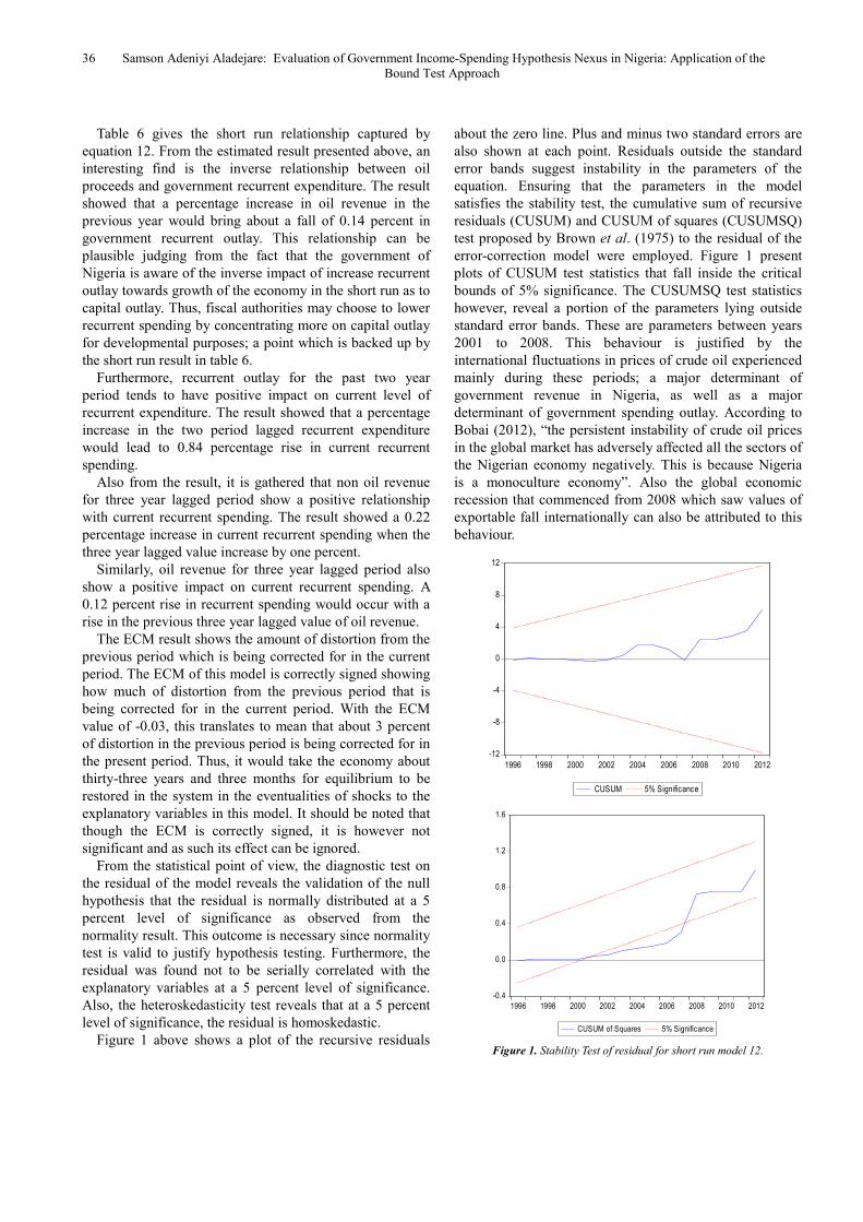
Figure 1 above shows a plot of the recursive residuals
about the zero line. Plus and minus two standard errors are
also shown at each point. Residuals outside the standard
error bands suggest instability in the parameters of the
equation. Ensuring that the parameters in the model
satisfies the stability test, the cumulative sum of recursive
residuals (CUSUM) and CUSUM of squares (CUSUMSQ)
test proposed by Brown et al. (1975) to the residual of the
error-correction model were employed. Figure 1 present
plots of CUSUM test statistics that fall inside the critical
bounds of 5% significance. The CUSUMSQ test statistics
however, reveal a portion of the parameters lying outside
standard error bands. These are parameters between years
2001 to 2008. This behaviour is justified by the
international fluctuations in prices of crude oil experienced
mainly during these periods; a major determinant of
government revenue in Nigeria, as well as a major
determinant of government spending outlay. According to
Bobai (2012), “the persistent instability of crude oil prices
in the global market has adversely affected all the sectors of
the Nigerian economy negatively. This is because Nigeria
is a monoculture economy”. Also the global economic
recession that commenced from 2008 which saw values of
exportable fall internationally can also be attributed to this
behaviour.
Figure 1. Stability Test of residual for short run model 12.
-12
-8
-4
0
4
8
12
1996 1998 2000 2002 2004 2006 2008 2010 2012
CUSUM 5% Significance
-0.4
0.0
0.4
0.8
1.2
1.6
1996 1998 2000 2002 2004 2006 2008 2010 2012
CUSUM of Squares 5% Significance
American Journal of Business, Economics and Management 2014, 2(1): 28-40 37
Table 7. Error Correction Representation for Equation13.
ARDL(1,0,0,0,0) selected based on AIC. Dependent variable : d(GCEXPt)
Regressor Coefficient Standard Error T- value Probability
C
dGREXP(-1)
dOREV(-1)
dGREXP(-2)
dNOREV(-2)
dOREV(-2)
dOREV(-3)
ECM(-1)
19792.11
-0.526356
0.052908
1.049689
-0.442005
-0.116753
0.224178
-0.238381
19061.58
0.237068
0.022095
0.225520
0.116764
0.044674
0.037870
0.139052
1.038325
-2.220271
2.394525
4.654535
-3.785442
-2.613431
5.919621
-1.714328
0.3129
0.0395**
0.0277**
0.0002***
0.0014***
0.0176**
0.0000***
0.1036*
R-Squared: 0.74 F-Statistic: 5.926248 Adjusted R-Squared: 0.62
Prob(F-Statistic): 0.000685 D-Watson stat: 2.384815
Diagnostic Tests of Residual.
Test Statistic LM Version F Version
Serial correlation
Normality
Heteroscedasticity
CHI2(3) =3.644712 [0.3025]
CHI2(3) =5.389023 [0.067575]
CHI2(9) = 6.394404 [0.6999]
F(3,15) = 0.748238 [0.5401]
Not Applicable
F(9,18) = 0.591921 [0.7873]
Note: ***, **, * represents significance at 1%, 5%, and 10% respectively.
Source: Computed by Author
The ECM result above shows that the one period lagged
values of GREXP and OREV affects the current levels of
GCEXP respectively. As expected, GREXP is inversely
related to GCEXP. From the result; it is obvious that a
percentage rise in GREXP in the previous year would lead
to 0.53 percentage fall in GCEXP in the present period.
This behaviour is true since an increase in either of GCEXP
OR GREXP in the short run, would cause a fall in the other
and vice versa. Also, a percent rise in OREV in the
previous period would yield a 0.05 percentage rise in
GCEXP for the current year. This behaviour is also true
since in Nigeria, government outlay for each year is being
determined by its oil sale revenue.
Furthermore, GREXP for the second year shows a
positive relationship with GCEXP which is unlike the
lagged by one result. From the result, it can be deduce that
a percentage increase in GREXP would yield 1.05
percentage rise in current level of GCEXP. Also, previous
two year value of NOREV shows an inverse relationship
with CEXP. This means a percentage increase NOREV in
the past two year would result in GCEXP falling by 0.44
percent in the current year. Furthermore, OREV for the past
two years show an inverse relationship with CEXP. The
result reveals that a percentage rise in the past two year
value of OREV would result in current level of CEXP
falling by 0.12 percent. This result is plausible given that in
government budgetary process in Nigeria, capital outlays of
government is being determined mostly by revenue
generated from immediate previous year oil sales.
For the three year lagged relationship between the
variables, it can be observed that an inverse relationship
exist between GREXP and GCEXP, and NOREV and
GCEXP respectively. Though both results are not
significant, the results reveals that a percentage increase in
GREXP would lead to a fall of 0.28 percent in GCEXP for
the current year. Likewise a percentage increase in NOREV
would result in 0.17 percent fall in GCEXP. However,
OREV in the third period shows a positive relationship
with GCEXP. The result reveals that an increase in OREV
by a percentage would lead to 0.22 percent rise in GCEXP
in the current year.
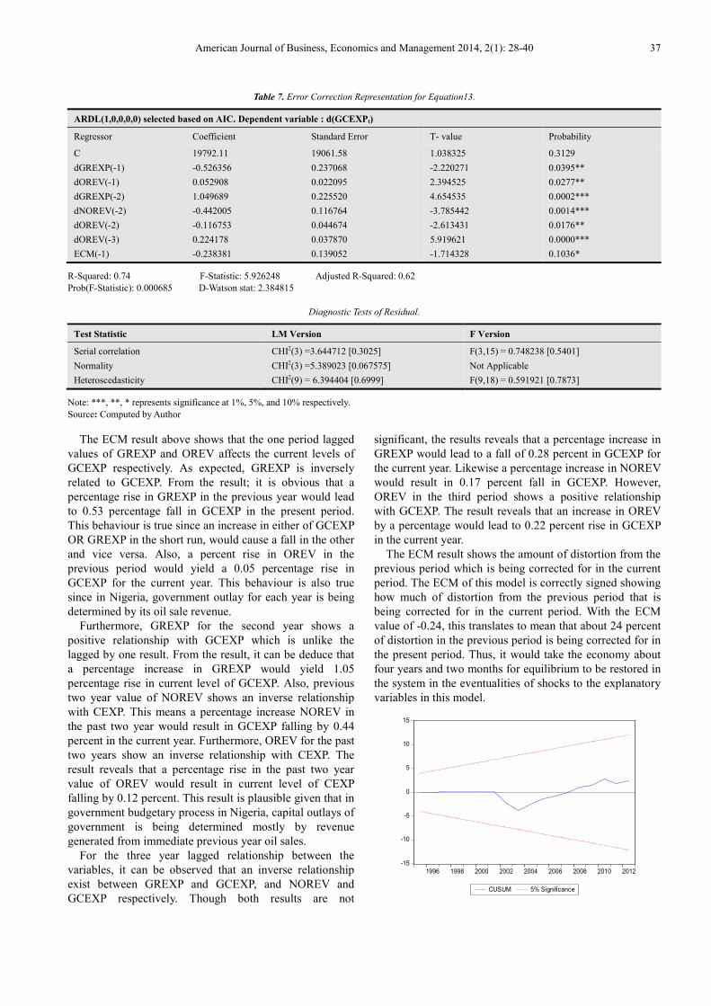
The ECM result shows the amount of distortion from the
previous period which is being corrected for in the current
period. The ECM of this model is correctly signed showing
how much of distortion from the previous period that is
being corrected for in the current period. With the ECM
value of -0.24, this translates to mean that about 24 percent
of distortion in the previous period is being corrected for in
the present period. Thus, it would take the economy about
four years and two months for equilibrium to be restored in
the system in the eventualities of shocks to the explanatory
variables in this model.
-15
-10
-5
0
5
10
15
1996 1998 2000 2002 2004 2006 2008 2010 2012
CUSUM 5% Significance
38 Samson Adeniyi Aladejare: Evaluation of Government Income-Spending Hypothesis Nexus in Nigeria: Application of the
Bound Test Approach
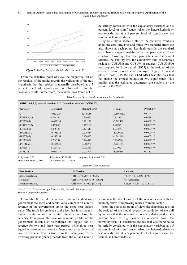
Figure 2. Stability Test of residual for short run model 13.
From the statistical point of view, the diagnostic test on
the residual of the model reveals the validation of the null
hypothesis that the residual is normally distributed at a 5
percent level of significance as observed from the
normality result. Furthermore, the residual was found not to
be serially correlated with the explanatory variables at a 5
percent level of significance. Also, the heteroskedasticity
test reveals that at a 5 percent level of significance, the
residual is homoskedastic.
Figure 2 above shows a plot of the recursive residuals
about the zero line. Plus and minus two standard errors are
also shown at each point. Residuals outside the standard
error bands suggest instability in the parameters of the
equation. Ensuring that the parameters in the model
satisfies the stability test, the cumulative sum of recursive
residuals (CUSUM) and CUSUM of squares (CUSUMSQ)
test proposed by Brown et al. (1975) to the residual of the
error-correction model were employed. Figure 1 present
plots of both CUSUM and CUSUMSQ test statistics that
fall inside the critical bounds of 5% significance. This
implies that the estimated parameters are stable over the
period 1981- 2012.
Table 8. Error Correction Representation for Equation14.
ARDL(1,0,0,0,0) selected based on AIC. Dependent variable : d(NOREVt)
Regressor Coefficient Standard Error T- value Probability
C
dGREXP(-1)
dCEXP(-1)
dGREXP(-2)
dCEXP(-2)
dNOREV(-2)
dREXP(-3)
dCEXP(-3)
dNOREV(-3)
dOREV(-3)
ECM(-1)
-6353.227
0.446704
-0.653133
1.037050
0.885488
-0.453386
-0.842153
0.764734
-0.595548
0.121412
-0.029179
12544.58
0.210525
0.121120
0.167187
0.127613
0.076584
0.176877
0.144447
0.088701
0.032639
0.022504
-0.5068452
2.121857
-5.392450
6.202951
6.938843
-5.920143
-4.761240
5.294216
-6.714134
3.719824
-1.296616
0.6194
0.0498**
0.0001***
0.0000***
0.0000***
0.0000***
0.0002***
0.0001***
0.0000***
0.0019***
0.2132
R-Squared: 0.97 F-Statistic: 45.28858 Adjusted R-Squared: 0.95
Prob(F-Statistic): 0.0000 D-Watson stat: 2.170189
Diagnostic Tests of Residual
Test Statistic LM Version F Version
Serial correlation
Normality
Heteroscedasticity
CHI2(3) =3.644712 [0.6332]
CHI2(3) =4.349660 [0.113627]
CHI2(9) = 7.653832 [0.7439]
F(3,13) = 0.123022 [0.7307]
Not Applicable
F(11,16) = 0.547172 [0.8431]
Note: ***, **, * represents significance at 1%, 5%, and 10% respectively.
Source: Computed by Author
From table 8, it could be gathered that in the short run,
government recurrent and capital outlay impact on non oil
revenue of the government up to the three year lagged
value. The result lay credence to the fact that investment in
human capital as well as capital infrastructure, have the
capacity to improve the non oil revenue profile of the
government. it can also be gathered that lagged non oil
revenue for two and three year period; while three year
lagged oil revenue also exact influence on current levels of
non oil revenue. This is true from the view point of re-
investing previous years proceeds from the oil and non oil
sector into the development of the non oil sector with the
main objective of improving returns from the sector.
From the statistical point of view, the diagnostic test on
the residual of the model reveals the validation of the null
hypothesis that the residual is normally distributed at a 5
percent level of significance as observed from the
normality result. Furthermore, the residual was found not to
be serially correlated with the explanatory variables at a 5
percent level of significance. Also, the heteroskedasticity
test reveals that at a 5 percent level of significance, the
residual is homoskedastic.
-0.4
0.0
0.4
0.8
1.2
1.6
1996 1998 2000 2002 2004 2006 2008 2010 2012
CUSUM of Squares 5% Significance
American Journal of Business, Economics and Management 2014, 2(1): 28-40 39
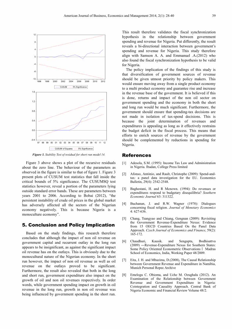
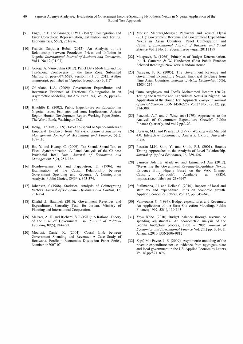
Figure 3. Stability Test of residual for short run model 14.
Figure 3 above shows a plot of the recursive residuals
about the zero line. The behaviour of the parameters as
observed in the figure is similar to that of figure 1. Figure 3
present plots of CUSUM test statistics that fall inside the
critical bounds of 5% significance. The CUSUMSQ test
statistics however, reveal a portion of the parameters lying
outside standard error bands. These are parameters between
years 2001 to 2006. According to Bobai (2012), “the
persistent instability of crude oil prices in the global market
has adversely affected all the sectors of the Nigerian
economy negatively. This is because Nigeria is a
monoculture economy”.
5. Conclusion and Policy Implication
Based on the study findings, this research therefore
concludes that although the impact of non oil revenue on
government capital and recurrent outlay in the long run
appears to be insignificant, as against the significant impact
oil revenue has on the outlays. This is obviously due to the
monocultural nature of the Nigerian economy. In the short
run however, the impact of non oil revenue as well as oil
revenue on the outlays proved to be significant.
Furthermore, the result also revealed that both in the long
and short run, government expenditure also impact on the
growth of oil and non oil revenues respectively. In order
words, while government spending impact on growth in oil
revenue in the long run, growth in non oil revenue was
being influenced by government spending in the short run.
This result therefore validates the fiscal synchronization
hypothesis in the relationship between government
spending and revenue for Nigeria. Put differently, the result
reveals a bi-directional interaction between government’s
spending and revenue for Nigeria. This study therefore
align with Samson A. A. and Emmanuel .A.(2012) who
also found the fiscal synchronization hypothesis to be valid
for Nigeria.
The policy implication of the findings of this study is
that diversification of government sources of revenue
should be given utmost priority by policy makers. This
would ensure moving away from a single product economy
to a multi product economy and guarantee rise and increase
in the revenue base of the government. It is believed if this
is done, returns and impact of the non oil sector on
government spending and the economy in both the short
and long run would be much significant. Furthermore, the
government should ensure that spending-tax decisions are
not made in isolation of tax-spend decisions. This is
because the joint determination of revenues and
expenditures is appealing as long as it effectively restrains
the budget deficit in the fiscal process. This means that
efforts to enrich sources of revenue by the government
should be complemented by reductions in spending for
Nigeria.
References
[1] Adesola, S.M. (1995): Income Tax Law and Administration in Nigeria. Ibadan, College Press limited
[2] Afonso, António, and Rault, Christophe (2009): Spend-and-tax: a panel data investigation for the EU. Economics Bulletin, 29(4): 2542-2548.
[3] Baghestani, H. and R Mcnown. (1994): Do revenues or expenditures respond to budgetary disequilibria? Southern Economic Journal 63: 311322.
[4] Buchanan, J. and R.W. Wagner (1978): Dialogues concerning fiscal religion. Journal of Monetary Economics 4: 627-636.
[5] Chang, Tsangyao and Chiang, Gengnan (2009): Revisiting the Government Revenue-Expenditure Nexus: Evidence from 15 OECD Countries Based On the Panel Data Approach. Czech Journal of Economics and Finance, 59(2): 165-172.
[6] Chaudhuri, Kausik. and Sengupta, Bodhisattva (2009) ―Revenue-Expenditure Nexus for Southern States: Some Policy Oriented Econometric Observations Madras ‖
School of Economics, India, Working Paper 48/2009.
[7] Eita, J. H. and Mbazima, D.(2008), The Causal Relationship between Government Revenue and Expenditure in Namibia, Munich Personal Repec Archive
[8] Emelogu C. Obioma, and Uche M. Ozughalu (2012). An Examination of the Relationship between Government Revenue and Government Expenditure in Nigeria: Cointegration and Causality Approach. Central Bank of Nigeria Economic and Financial Review Volume 48/2.
-12
-8
-4
0
4
8
12
1996 1998 2000 2002 2004 2006 2008 2010 2012
CUSUM 5% Significance
-0.4
0.0
0.4
0.8
1.2
1.6
97 98 99 00 01 02 03 04 05 06 07 08 09 10 11 12
CUSUM of Squares 5% Significance
40 Samson Adeniyi Aladejare: Evaluation of Government Income-Spending Hypothesis Nexus in Nigeria: Application of the
Bound Test Approach
[9] Engel, R. F. and Granger, C.W.J. (1987): Cointegration and Error Correction: Representation, Estimation and Testing. Econometrica, 55(2), 251-276.
[10] Francis Danjuma Bobai (2012). An Analysis of the Relationship between Petroleum Prices and Inflation in Nigeria. International Journal of Business and Commerce. Vol 1, No 12 (01-07)
[11] George A. Vamvoukas (2012). Panel Data Modeling and the Tax-Spend Controversy in the Euro Zone. Submitted Manuscript peer-00716629, version 1-11 Jul 2012. Author manuscript, published in "Applied Economics (2011)"
[12] Gil-Alana, L.A. (2009): Government Expenditures and Revenues: Evidence of Fractional Cointegration in an Asymmetric Modeling. Int Adv Econ Res, Vol.15, pp:143–155.
[13] Hincliffe K. (2002). Public Expenditure on Education in Nigeria: Issues, Estimates and some Implications. African Region Human Development Report Working Paper Series. The World Bank, Washington D.C.
[14] Hong, Tan Juat (2009): Tax-And-Spend or Spend-And-Tax? Empirical Evidence from Malaysia. Asian Academy of Management Journal of Accounting and Finance, 5(1): 107–115.
[15] Ho, Y. and Huang, C. (2009). Tax-Spend, Spend-Tax, or Fiscal Synchronization: A Panel Analysis of the Chinese Provincial Real Data. Journal of Economics and Management, 5(2), 257-272.
[16] Hondroyiannis, G. and Papapetrou, E. (1996). An Examination of the Causal Relationship between Government Spending and Revenue: A Cointegration Analysis. Public Choice, 89(3/4), 363-374.
[17] Johansen, S.(1988). Statistical Analysis of Cointegrating Vectors. Journal of Economic Dynamics and Control, 12, 231-254.
[18] Khalid .I. Bataineh (2010): Government Revenues and Expenditures: Causality Tests for Jordan. Ministry of Planning and International Cooperation.
[19] Meltzer, A. H. and Richard, S.F. (1981): A Rational Theory of the Size of Government. The Journal of Political Economy, 89(5), 914-927.
[20] Moalusi, Daniel K. (2004): Causal Link between Government Spending and Revenue: A Case Study of Botswana. Fordham Economics Discussion Paper Series, Number dp2007-07.
[21] Mohsen Mehrara,Mosayeb Pahlavani and Yousef Elyasi (2011): Government Revenue and Government Expenditure Nexus in Asian Countries: Panel Cointegration and Causality. International Journal of Business and Social Science Vol. 2 No. 7; [Special Issue –April 2011] 199
[22] Musgrave, R. (1966): Principles of Budget Determination. In: H. Cameron & W. Henderson (Eds) Public Finance: Selected Readings. New York: Random House.
[23] Narayan, P. K. (2005): The Government Revenue and Government Expenditure Nexus: Empirical Evidence from Nine Asian Countries. Journal of Asian Economies, 15(6), 1203-1216.
[24] Omo Aregbeyen and Taofik Mohammed Ibrahim (2012). Testing the Revenue and Expenditure Nexus in Nigeria: An Application of the Bound Test Approach. European Journal of Social Sciences ISSN 1450-2267 Vol.27 No.3 (2012), pp. 374-380.
[25] Peacock, A.T. and J. Wiseman (1979): Approaches to the Analysis of Government Expenditure Growth", Public Finance Quarterly, and vol.7 pp.3-23.
[26] Pesaran, M.H and Pesaran B. (1997). Working with Microfit 4.0: Interactive Econometric Analysis. Oxford University Press.
[27] Pesaran M.H, Shin, Y., and Smith, R.J. (2001). Bounds Testing Approaches to the Analysis of Level Relationship. Journal of Applied Economics, 16: 289-326.
[28] Samson Adeniyi Aladejare and Emmanuel Ani (2012). “Revisiting the Government Revenue-Expenditure Nexus: Evidence from Nigeria Based on the VAR Granger Causality Approach”. Available at SSRN: http://ssrn.com/abstract=2186947
[29] Stallmanna, J.I. and Deller S. (2010): Impacts of local and state tax and expenditure limits on economic growth. Applied Economics Letters, Vol. 17, pp: 645–648.
[30] Vamvoukas G. (1997): Budget expenditures and Revenues: An Application of the Error Correction Modeling; Public Finance; 1997, 52(1), 139-143
[31] Yaya Keho (2010) Budget balance through revenue or spending adjustments? An econometric analysis of the Ivorian budgetary process, 1960 – 2005 Journal of Economics and International Finance Vol. 2(1) pp. 001-011 Janauary,2010.ISSN2006-9812.
[32] Zapf, M.; Payne, J. E. (2009): Asymmetric modeling of the revenue-expenditure nexus: evidence from aggregate state and local government in the US. Applied Economics Letters, Vol.16,pp:871–876.
Related Documents


