Evaluation of EGM2008 within geopotential space from GPS, tide Gauges and altimetry

1

2 Evaluation of EGM2008 Within3 Geopotential Space from GPS,4 Tide Gauges and Altimetry

39

5 N. Dayoub, P. Moore, N.T. Penna, and S.J. Edwards

6 Abstract

7 The new global Earth gravitational model EGM2008 has been evaluated within

8 geopotential space by comparison with its predecessor EGM96 and the GRACE

9 combination model EIGEN-GL04C. The methodology comprises establishing

10 geodetic coordinates of mean sea level (MSL) from GPS observations, tide

11 gauge (TG) time series and levelling. The gravity potential at MSL was estimated

12 at each TG location by utilising the ellipsoidal harmonic coefficients of the

13 adopted gravity field models to their maximum degree and order. This study

14 uses data from 23 TGs around the Baltic Sea, nine in the UK and one in France.

15 Comparison involves testing the agreement between geopotential values for each

16 country as gravity potentials at MSL are supposed to be consistent for regions

17 where mean dynamic topography (MDT) does not differ significantly. Results

18 show significant improvement with the EGM2008 model compared against its

19 counterparts. The study shows the effect of omission errors on the solution by

20 limiting the EGM2008 model to maximum degree and order 360 in the regional

21 study. In addition to the regional study, EGM2008 was also evaluated globally

22 using MSL derived from altimetric data. The global study shows that W0, the

23 potential value on the geoid, is not affected by high degree terms of the

24 EGM2008.

39.125 Introduction

26 A new ultra high degree combination Earth gravita-

27 tional model EGM2008 (Pavlis et al. 2008) has been

28 released by the EGM development team of the

29 National Geospatial-Intelligence Agency (NGA).

30 This model consists of a complete set of spherical

31harmonics up to degree/order 2159/2159 (4670000

32coefficients) and is further extended by additional

33harmonics to degree 2190 and order 2159. The

34model yields gravity effects of features larger than

359 km. EGM2008 is based on gravitational information

36from GRACE and incorporates 50 � 50 global gravity37anomalies. Coefficients of this model are freely avail-

38able (http://earth-info.nga.mil/GandG/).

39In this study, EGM2008 has been tested within

40geopotential space against the European Improved

41Gravity model of the Earth by New techniques

42(EIGEN-GL04C) (F€orste et al. 2006) and the

43EGM96 model (Lemoine et al. 1998) which consist

N. Dayoub (*) � P. Moore � N.T. Penna � S.J. EdwardsSchool of Civil Engineering and Geosciences, Newcastle

University, Newcastle NE1 7RU, UK

e-mail: [email protected]

S. Kenyon et al. (eds.), Geodesy for Planet Earth, International Association of Geodesy Symposia 136,

DOI 10.1007/978-3-642-20338-1_39, # Springer-Verlag Berlin Heidelberg 2011

321

44 of coefficients only up to degree and order 360. Eval-

45 uation involves establishing the geodetic coordinates

46 of MSL at TGs and estimating the gravity potential at

47 these points. The gravity potentials at MSL should be

48 consistent in countries or regions where the effects of

49 MDT are small. This is particularly applicable when

50 oceanographic and meteorological effects such as

51 ocean currents, atmospheric pressure and winds are

52 similar such as in a semi-enclosed sea. As proof that

53 MDT is small over the study region, 120 monthly

54 means of the Simple Ocean Data Assimilation Analy-

55 sis (SODA) MDT model (Carton et al. 2000) were

56 analysed. This showed that MDT does not vary by

57 more than 10 cm within any of the individual countries

58 involved in this study. Thus, the improvement of the

59 gravity model can be detected from the increased

60 agreement between the results for each country. It is

61 noted that a global gravity model (GGM) to degree

62 and order 360 would only cover gravity features larger

63 than 55 km. This may not provide a sufficiently accu-

64 rate solution for local or regional work as a result of

65 the omission of coefficients of degree greater than 360.

66 In addition to the regional approach, EGM2008 has

67 also been evaluated globally using MSL derived from

68 satellite altimetry. In particular, the effect of omission

69 errors and the use of a globalMDTmodel are investigated.

39.270 Data: Regional Analysis

71 The TGs used for the regional analysis are shown in

72 Fig. 39.1. 23 of the TGs are situated around the Baltic

73 Sea, namely four in Germany (GER), eight in Finland

74 (FIN), two in Lithuania (LIT), two in Poland

75 (POL) and seven in Sweden (SWE). These TGs are

76 connected to the geocentre by means of episodic

77 GPS observations which were collected in 1993.4

78 and 1997.4 as a part of the Baltic sea level project

79 (Poutanen and Kakkuri 1999), with geocentric co-

80 ordinates given in Ardalan et al. (2002). All GPS

81 heights were used from the later campaign except for

82 Swinoujscie in Poland the 1993.4 value was used as

83 the site was not occupied in 1997.4. Unlike the other

84 Baltic Sea TGs, three of the German TGs are located

85 on the North Sea with the other in the Danish channel.

86 This study also uses data from nine UK TGs and one in

87 France (Brest), all of which are co-located with con-

88 tinuously operating GPS (CGPS) receivers. Precise

89 levelling was used to connect the GPS and TG datums.

90To calculate the geodetic coordinates of the UK and

91Brest CGPS stations, 1 year of GPS data from 2006

92were analysed using GIPSY-OASIS 5.0 software in

93precise point positioning mode (Zumberge et al.

941997). The data were processed in 24 h sessions: JPL

95reprocessed non-fiducial orbits, satellite clocks and

96Earth rotation parameters were held fixed. Models

97were applied for absolute transmitter and receiver

98antenna phase centre variations (Schmid et al. 2007);

99Earth body tides according to the IERS 2003

100conventions (McCarthy and Petit 2004); and ocean

101tide loading using the FES2004 model

102Lyard et al. (2006), computed via www.oso.chalm

103ers.se/~loading. Wet tropospheric zenith delays and

104north-south and east-west horizontal gradients were

105estimated every 5 min while the VMFI mapping func-

106tion was used (Boehm et al. 2006) together with an

107elevation angle cut-off 10 degrees. Ambiguities were

108fixed via ambizap (Blewitt 2008). The non fiducial

109daily coordinates were transformed to ITRF2005

110with the final height estimates taken as the mean

111values for the whole of 2006.

112Mean monthly data files for the UK/France TGs

113were selected in Revised Local Reference (RLR)

114format from the Permanent Service for Mean Sea

115Level (PSMSL). The chosen stations have a mini-

116mum of 30 full years of sea level data, which is

117needed to determine secular MSL changes precise

118to 0.5 mm/year (Woodworth et al. 1999), while 50

119years of data increase the precision to 0.3 mm/year

120(Douglas 1991). For each TG time series the mean

121and trend were estimated along with annual, semi-

122annual and 18.6 year tidal signals. The mean was

123moved to year 2006.5 to correspond to the GPS

124epoch using (39.1)

TGRt ¼ TGR0 þ ðt� t0Þ � tnd (39.1)

125where t corresponds to 2006.5 , TGRt is the value of

126the TG record at the time t, t0 refers to the reference

127time for TGR0, and tnd the annual MSL trend at the

128TG. It is assumed here that the principle change in the

129TG time series is caused by secular changes in the sea

130level and land movement due to global isostatic

131adjustment (GIA). Both can be considered secular on

132a short time scale as in this study although one can not

133exclude the possibility of non-linear changes due

134localised movement and an acceleration in sea level

135change.

322 N. Dayoub et al.

39.3136 Methodology: Regional Analysis

137 The methodology involves constructing the geodetic

138 coordinates of MSL at the TG. The geodetic latitude

139 and longitude were obtained directly from the GPS

140 analysis, while the geoid heights were obtained from

141 (39.2) which is illustrated in Fig. 39.2

N ¼ hþ TGR� ðDH þ HTGÞ: (39.2)

142 In (39.2) MDT has been neglected; thus MSL

143 approximate the geoid. The potential value on the

144 geoid is given by

W0ð’; l; NÞ ¼ Vð’; l; NÞ þ F ð’; NÞ (39.3)

145 where V is the gravitational potential, the centrifugal

146 potential and j, l and N the geodetic latitude, longi-

147 tude and height of the point corresponding to MSL.

148 The World Geodetic Datum 2000 (WGD2000) was

149 used as the reference ellipsoid with a ¼150 6378136.701 m and b ¼ 6356751.661 m in the mean

151 tide system (Ardalan and Grafarend 2000). The GGMs

152 were also transformed into the mean tide system as far

153as the permanent tide was concerned to maintain con-

154sistency with the reference ellipsoid. As this work is

155part of a more extensive study using the normal grav-

156ity field we made use of the representation of the

157Earth’s gravity field in terms of ellipsoidal coefficients

158(Ardalan et al. 2002). Although the study could have

159use the standard spherical harmonics we note here that

160ellipsoidal harmonics do not suffer from the ultra high

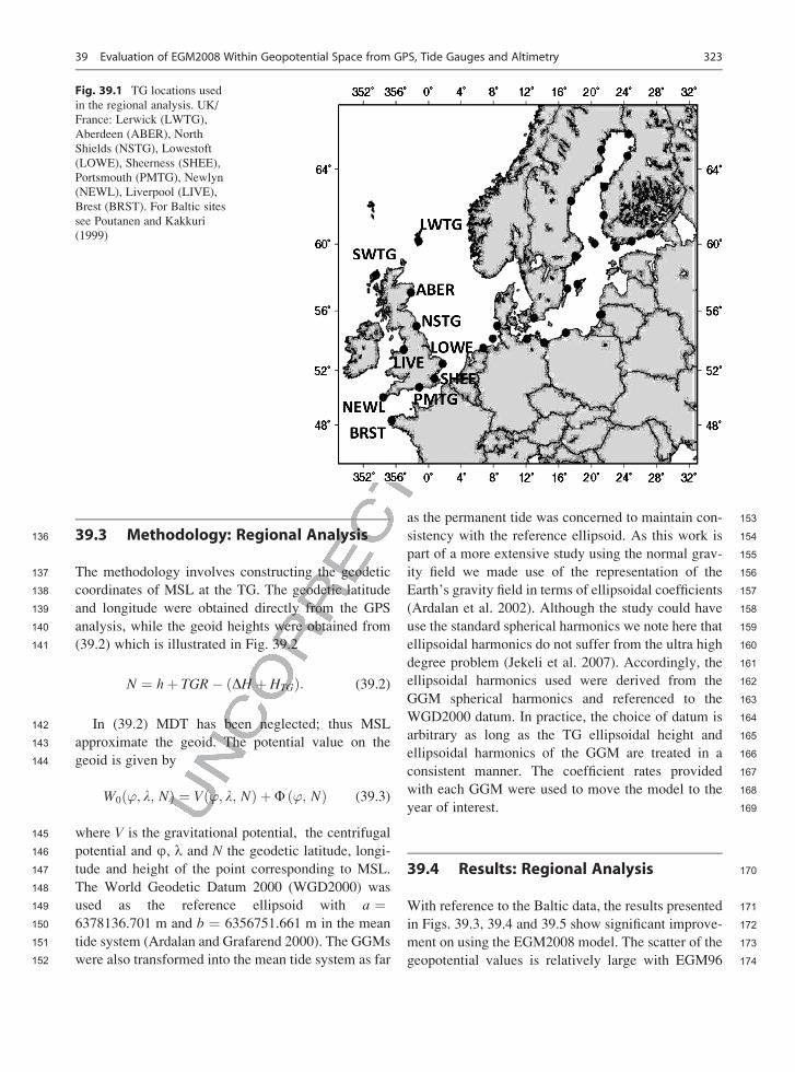
161degree problem (Jekeli et al. 2007). Accordingly, the

162ellipsoidal harmonics used were derived from the

163GGM spherical harmonics and referenced to the

164WGD2000 datum. In practice, the choice of datum is

165arbitrary as long as the TG ellipsoidal height and

166ellipsoidal harmonics of the GGM are treated in a

167consistent manner. The coefficient rates provided

168with each GGM were used to move the model to the

169year of interest.

39.4 170Results: Regional Analysis

171With reference to the Baltic data, the results presented

172in Figs. 39.3, 39.4 and 39.5 show significant improve-

173ment on using the EGM2008 model. The scatter of the

174geopotential values is relatively large with EGM96

Fig. 39.1 TG locations used

in the regional analysis. UK/

France: Lerwick (LWTG),

Aberdeen (ABER), North

Shields (NSTG), Lowestoft

(LOWE), Sheerness (SHEE),

Portsmouth (PMTG), Newlyn

(NEWL), Liverpool (LIVE),

Brest (BRST). For Baltic sites

see Poutanen and Kakkuri

(1999)

39 Evaluation of EGM2008 Within Geopotential Space from GPS, Tide Gauges and Altimetry 323

175 and EIGEN-GL04C, while the results become more

176 consistent with EGM2008. In particular, there is

177 enhanced agreement when comparing values for each

178 country separately. The results are particularly

179 improved at Ustka in Poland which is highlighted

180 with a circle in Fig. 39.3. This was considered as an

181 outlier with the EGM96 model and with a clear offset

182of 4 m2s�2 from the other Polish station on using the

183EIGEN-GL04C model. In Fig. 39.5, the German

184stations possess higher geopotential values than the

185other Baltic countries. This is due to the German

186stations being exposed to North Sea MDT that is

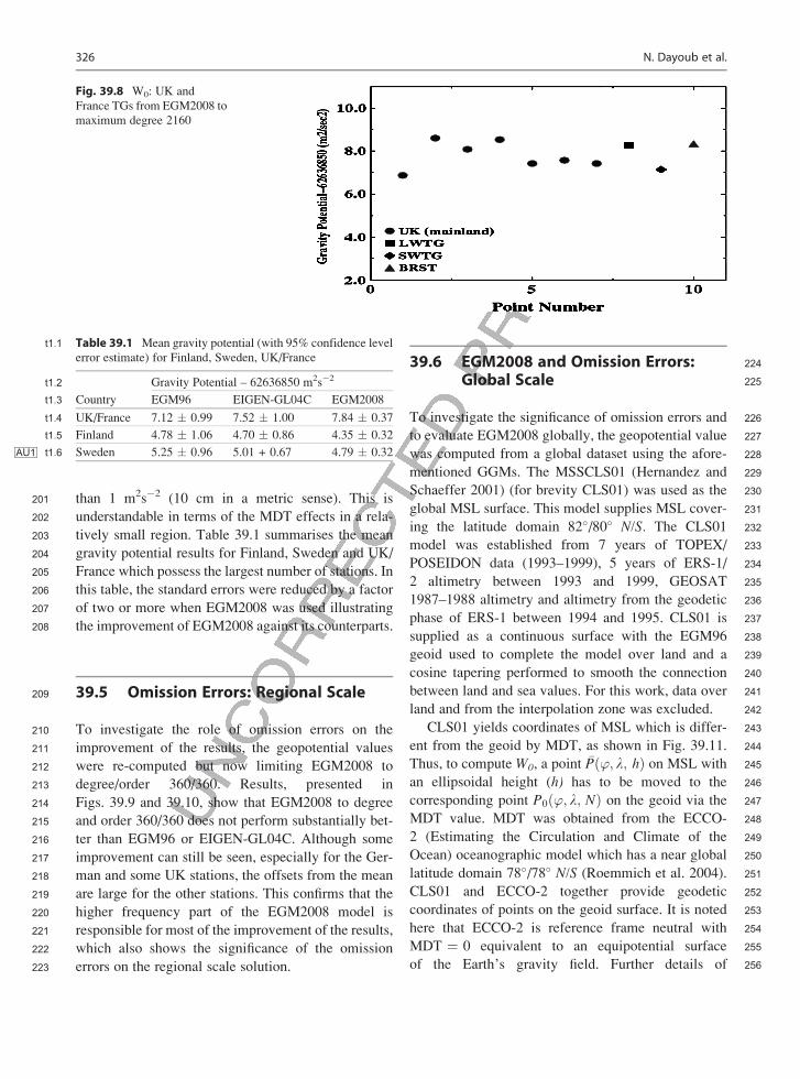
187distinct in its nature from the sites in the enclosed

188Baltic Sea.

Ellipsoid

Sea floor

MSL

h: Ellipsoidal height;N: Geoid height;

TG Zero

TG

TGR

TGR: Tide gauge reading.

HTG

HTG: Height of TG above the TG zero level;

H

Nh

GPSH: Height difference between GPS and TG;

Fig. 39.2 Geoid height from

GPS and TG

Fig. 39.3 W0: Baltic TGs

from EGM96: Ustka (Poland)

circled


from EIGEN-GL04C


189 A similar improvement accrued when processing

190 the UK and Brest (BRST) data which were referenced

191 to year 2006.5. Here, the UK is divided into three

192 regions according to the underlying height datum,

193 UK mainland (England, Scotland and Wales), Lerwick

194 (LWTG), Stornoway (SWTG). As shown in Figs. 39.6,

19539.7 and 39.8 the EGM2008 model has given consis-

196tency to all geopotential values over the entire area

197especially for the Stornoway value which was consid-

198ered as an outlier with the other gravity models. Fur-

199thermore, results from EGM2008 over the UK and

200Baltic areas seem to depart from the mean by less


from EGM2008 to maximum

degree 2160

Fig. 39.6 W0: UK and

France TGs from EGM96


France TGs from EGEN-

GL04C


201 than 1 m2s�2 (10 cm in a metric sense). This is

202 understandable in terms of the MDT effects in a rela-

203 tively small region. Table 39.1 summarises the mean

204 gravity potential results for Finland, Sweden and UK/

205 France which possess the largest number of stations. In

206 this table, the standard errors were reduced by a factor

207 of two or more when EGM2008 was used illustrating

208 the improvement of EGM2008 against its counterparts.

39.5209 Omission Errors: Regional Scale

210 To investigate the role of omission errors on the

211 improvement of the results, the geopotential values

212 were re-computed but now limiting EGM2008 to

213 degree/order 360/360. Results, presented in

214 Figs. 39.9 and 39.10, show that EGM2008 to degree

215 and order 360/360 does not perform substantially bet-

216 ter than EGM96 or EIGEN-GL04C. Although some

217 improvement can still be seen, especially for the Ger-

218 man and some UK stations, the offsets from the mean

219 are large for the other stations. This confirms that the

220 higher frequency part of the EGM2008 model is

221 responsible for most of the improvement of the results,

222 which also shows the significance of the omission

223 errors on the regional scale solution.

39.6 224EGM2008 and Omission Errors:225Global Scale

226To investigate the significance of omission errors and

227to evaluate EGM2008 globally, the geopotential value

228was computed from a global dataset using the afore-

229mentioned GGMs. The MSSCLS01 (Hernandez and

230Schaeffer 2001) (for brevity CLS01) was used as the

231global MSL surface. This model supplies MSL cover-

232ing the latitude domain 82�/80� N/S. The CLS01

233model was established from 7 years of TOPEX/

234POSEIDON data (1993–1999), 5 years of ERS-1/

2352 altimetry between 1993 and 1999, GEOSAT

2361987–1988 altimetry and altimetry from the geodetic

237phase of ERS-1 between 1994 and 1995. CLS01 is

238supplied as a continuous surface with the EGM96

239geoid used to complete the model over land and a

240cosine tapering performed to smooth the connection

241between land and sea values. For this work, data over

242land and from the interpolation zone was excluded.

243CLS01 yields coordinates of MSL which is differ-

244ent from the geoid by MDT, as shown in Fig. 39.11.

245Thus, to compute W0, a point �Pð’; l; hÞ on MSL with

246an ellipsoidal height (h) has to be moved to the

247corresponding point P0ð’; l; NÞ on the geoid via the

248MDT value. MDT was obtained from the ECCO-

2492 (Estimating the Circulation and Climate of the

250Ocean) oceanographic model which has a near global

251latitude domain 78�/78� N/S (Roemmich et al. 2004).

252CLS01 and ECCO-2 together provide geodetic

253coordinates of points on the geoid surface. It is noted

254here that ECCO-2 is reference frame neutral with

255MDT ¼ 0 equivalent to an equipotential surface

256of the Earth’s gravity field. Further details of


France TGs from EGM2008 to

maximum degree 2160

t1:1 Table 39.1 Mean gravity potential (with 95% confidence level

error estimate) for Finland, Sweden, UK/France

Gravity Potential – 62636850 m2s�2t1:2

Country EGM96 EIGEN-GL04C EGM2008t1:3

UK/France 7.12 � 0.99 7.52 � 1.00 7.84 � 0.37t1:4

Finland 4.78 � 1.06 4.70 � 0.86 4.35 � 0.32t1:5

Sweden 5.25 � 0.96AU1 5.01 + 0.67 4.79 � 0.32t1:6


257 oceanographic model reference frames are given in

258 (Hughes and Bingham 2008). Data between 70�/70�

259 N/S were employed for this study. We computed

260 geopotential values on a 1 � 1 latitude/longitude

261 grid by expanding EGM96, EIGEN-GL04C and

262 EGM2008 to degree/order 360/360 and EGM2008 to

263degree/order 2160/2160. As before the GGMs were

264transformed into the mean tide system. The gravity

265potential was determined at each grid point of

266the CLS01 model, with the equi-area weighted aver-

267age used to estimate W0. Table 39.2 shows W0 values

268with 95% confidence level error estimation before and

269after accounting for MDT.

270The results, summarised in Table 39.2, show that

271the global value of W0 is essentially invariant with


from EGM2008 to maximum

degree 360


France TGs from EGM2008 to

maximum degree 360

Fig. 39.11 Geoid height (N) from ellipsoidal height (h) andMDT

t2:1Table 39.2 The effect on W0 of using different GGMs and

maximum degree (n) (with 95% confidence level error estimate)

based on CLS01 (70�/70� N/S) with/without correction for MDT

from ECCO-2

GGM n W0 – 62636850 m2s�2 t2:2

CLS01 CLS01 and ECCO-2 t2:3

EGM96 360 4.30 � 0.07 4.34 � 0.03 t2:4

EIGEN-GL04C 360 4.27 � 0.07 4.30 � 0.03 t2:5

EGM2008 360 4.25 � 0.06 4.29 � 0.02 t2:6

EGM2008 2,160 4.25 � 0.06 4.29 � 0.02 t2:7


272 the GGM. Furthermore, EGM2008 to degree/order

273 2160/2160 gave exactly the same value W0 as that

274 from the field truncated at degree and order 360.

275 Although removing MDT has only a small effect on

276 W0, consideration of MDT has halved the standard

277 errors for EGM96 and EIGEN-GL04C, and reduced

278 the standard error by two thirds for EGM2008. Fur-

279 thermore, EGM2008 has the lowest standard error

280 which reflects an improvement in this model. The

281 consistency between the GGMs and the agreement

282 between the full and truncated EGM2008 fields

283 shows that omission errors after a certain degree/

284 order do not influence W0 globally. Accordingly, a

285 high resolution GGM is not necessary for estimating

286 W0. To find the minimum degree required of the GGM

287 after which the omission errors are not significant, W0

288 was estimated with EGM2008 with truncation at vari-

289 ous degrees (n). Figure 39.12 shows that the

290 geopotential values converge approximately at degree

291 80-100, while after n ¼ 120, there is practically no

292 difference in W0. Thus, a GGM to degree 120 is

293 sufficient to estimate W0 at the global scale. This

294 enables the possibility to determine W0 from a satel-

295 lite-only Earth gravity field model such as EIGEN-

296 GL04S1 (F€orste et al. 2006). It is noted, however,

297 that the Sanchez (2008) showed that W0 is dependent

298 on the latitude band over which W0 was estimated.

299 Conclusions300

301 The performance of the EGM2008 gravity field

302 model was evaluated within geopotential space

303 over five Baltic countries, the UK and France. It

304 appears that, the use of EGM2008 has significantly

305 increased the consistency of the gravity potentials

306at MSL for the countries involved (see Table 39.1).

307It was seen that omission errors are the main reason

308for the large offsets between the geopotential

309values at local and regional scales. Additional

310studies extending the regional network used

311here is necessary to provide further validation of

312EGM2008.

313Globally, all GGM’s give essentially the same

314results within the standard errors (see Table 39.2).

315However, of more significance is the use of a MDT

316model. The results show that, at the global scale,

317the high frequency part of EGM2008 has a negligi-

318ble effect on W0.

Acknowledgements The authors would like to thank the fol-

319lowing institutions for supplying data for this study: NASA JPL

320for GIPSY software and the provision of orbital products, NERC

321BIGF for GPS data at UK tide gauge sites and EUREF/IGS for

322Brest GPS data.

323References

324Ardalan A, Grafarend E, Kakkuri J (2002) National height

325datum, the Gauss-Listing geoid level value W0 and its time

326variation W0 (Baltic Sea Level project: epochs 1990.8,

3271993.8, 1997.4). J Geodesy 76(1):1–28

328Ardalan AA, Grafarend EW (2000) Reference ellipsoidal grav-

329ity potential field and gravity intensity field of degree/order

330360/360 (manual of using ellipsoidal harmonic coefficients

331ellipfree.dat and ellipmean.dat). http://www.uni-stuttgart.de/

332gi/research/index.html#projects

333Blewitt G (2008) Fixed point theorems of GPS carrier phase

334ambiguity resolution and their application to massive net-

335work processing: Ambizap. J Geophys Res B Solid Earth

336113(12)

0

9

8

7

6

5W0-

6263

6850

(m

2/se

c2)

4100 200

Degree (n)300 400

Fig. 39.12 Dependence of

W0 on maximum degree n of

the GGM (GGM: EGM2008,

MSS: CLS01)


337 Boehm J, Werl B, Schuh H (2006) Troposphere mapping

338 functions for GPS and very long baseline interferometry

339 from European Centre for Medium-Range Weather Forecasts

340 operational analysis data. J Geophys Res B Solid Earth 111(2)

341 Carton JA, Chepurin G, Cao X, Giese B (2000) A simple ocean

342 data assimilation analysis of the global upper ocean 1950-95.

343 Part I: methodology. J Phys Oceanogr 30(2):294–309

344 Douglas BC (1991) Global sea level rise. J Geophys Res 96

345 (C4):6981–6992

346 F€orste C, Flechtner F, Schmidt R, K€onig R, Meyer U, Stubenvoll

347 R, Rothacher M, Barthelmes F, Neumayer H, Biancale R

348 (2006) A mean global gravity field model from the combina-

349 tion of satellite mission and altimetry/gravimetry surface

350 data: EIGEN-GL04C. Geophys Res Abstr 8:03462

351 Hernandez F, Schaeffer P (2001) The CLS01 mean sea surface:

352 a validation with the GSFC00 surface. press, CLS

353 Ramonville StAgne, France

354 Hughes CW, Bingham RJ (2008) An oceanographer’s guide to

355 GOCE and the geoid. Ocean Sci 4(1):15–29

356 Jekeli C, Lee JK, Kwon JH (2007) On the computation and

357 approximation of ultra-high-degree spherical harmonic

358 series. J Geodesy 81(9):603–615

359 Lemoine FG, Kenyon SC, Factor JK, Trimmer RG, Pavlis NK,

360 Chinn DS, Cox CM, Klosko SM, Luthcke SB, Torrence MH

361 (1998) The Development of the Joint NASA GSFC and

362 the National Imagery and Mapping Agency(NIMA)

363 Geopotential Model EGM 96. NASA, (19980218814)

364Lyard F, Lefevre F, Letellier T, Francis O (2006) Modelling the

365global ocean tides: modern insights from FES2004. Ocean

366Dyn 56(5–6):394–415

367McCarthy DD, Petit G (2004) IERS Conventions 2003. IERS

368Technical Note, 32, p 127

369Pavlis N, Kenyon S, Factor J, Holmes S (2008) Earth gravita-

370tional model 2008. In SEG Technical Program Expanded

371Abstracts, vol 27, pp 761–763

372PoutanenM, Kakkuri J (1999) Final results of the Baltic Sea level

3731997 GPS Campaign. Rep Finnish Geodetic Institute. 99(2)

374Roemmich D, Riser S, Davis R, Desaubies Y (2004) Autono-

375mous profiling floats: workhorse for broadscale ocean

376observations. J Mar Technol Soc 38:31–39

377Sanchez L (2008) Approach for the establishment of a global

378vertical reference level. In: Proceedings of the VI Hotine-

379Marussi Symposium, Springer, May 2008

380Schmid R, Steigenberger P, Gendt G, Ge M, Rothacher M

381(2007) Generation of a consistent absolute phase-center cor-

382rection model for GPS receiver and satellite antennas.

383J Geodesy 81(12):781–798

384Woodworth PL, Tsimplis MN, Flather RA, Shennan I (1999) A

385review of the trends observed in British Isles mean sea level

386data measured by tide gauges. Geophys J Int 136(3):651–670

387Zumberge JF, Heflin MB, Jefferson DC, Watkins MM, Webb

388FH (1997) Precise point positioning for the efficient and

389robust analysis of GPS data from large networks. J Geophys

390Res 102:5005–5017


Author QueriesChapter No.: 39

Query Refs. Details Required Author’s response

AU1 Should “5.01 + 0.67” be “5.01 � 0.67”? Please clarify.

Evaluation of EGM2008 within geopotential space from GPS, tide Gauges and altimetry

Documents