Evaluation of dynamical models: Dissipative synchronization and other techniques

Evaluation of dynamical models: Dissipative synchronization and other techniques

Luis Antonio Aguirre,* Edgar Campos Furtado, and Leonardo A. B. TôrresLaboratório de Modelagem, Análise e Controle de Sistemas Não-Lineares, Programa de Pós-Graduação em Engenharia Elétrica,

Universidade Federal de Minas Gerais, Avenue Antônio Carlos 6627, 31270-901 Belo Horizonte, Minas Gerais, Brazil�Received 15 September 2005; revised manuscript received 28 August 2006; published 13 December 2006�

Some recent developments for the validation of nonlinear models built from data are reviewed. Besidesgiving an overall view of the field, a procedure is proposed and investigated based on the concept of dissipativesynchronization between the data and the model, which is very useful in validating models that should repro-duce dominant dynamical features, like bifurcations, of the original system. In order to assess the discriminat-ing power of the procedure, four well-known benchmarks have been used: namely, Duffing-Ueda, Duffing-Holmes, and van der Pol oscillators, plus the Hénon map. The procedure, developed for discrete-time systems,is focused on the dynamical properties of the model, rather than on statistical issues. For all the systemsinvestigated, it is shown that the discriminating power of the procedure is similar to that of bifurcationdiagrams—which in turn is much greater than, say, that of correlation dimension—but at a much lowercomputational cost.

DOI: 10.1103/PhysRevE.74.066203 PACS number�s�: 05.45.Tp, 05.45.Xt, 07.05.Tp, 07.05.Kf

I. INTRODUCTION

Model building from data has been of great interest formany years within the community of nonlinear dynamicssince one of the first works in this field �1�. For the last 20years or so, many different procedures have been put forwardfor building nonlinear models from data. In a sense, the fieldof model building is now rather mature within the commu-nity of nonlinear dynamics.

After building a model it is important to know if such amodel is in fact a dynamical analog of the original system.An answer to that question is searched for during modelvalidation. Among the several issues concerning modelbuilding, model validation is probably the one that has re-ceived the least attention. For instance, in �2� an interestingdiscussion of several aspects of global modeling is found;however, model validation is hardly mentioned.

Many of the tools for model validation that were com-monly used by the mid-1990s were investigated and com-pared in �3�. The main conclusion of such a work was that ifa global model of a system is required, then one of the mostexacting procedures for model validation is to compare themodel bifurcation diagram to that of the true system. Twosimilar diagrams1 point to two entities �usually system andmodel� which display the same dynamical regimes over arather wide range of parameter values. In fact it is widelyacknowledged that bifurcation diagrams “are one of the mostinformative forms of presentation of dynamical evolution”�4�. On the other hand, quantities such as dimension mea-sures, Lyapunov exponents, phase portraits, and so on canonly quantify attractors and actually say very little about the

model ability to mimic the system as it evolves from onedynamical regime �attractor� to another. Thus, good modelsshould match closely such geometrical invariants; however,that matching is insufficient on its own to guarantee the qual-ity of such models �5�. In fact, it is known that even twodrastically different attractors may have similar fractal di-mension or Lyapunov exponents.

Although bifurcation diagrams provide a very exactingmeans of verifying the dynamical overall behavior of amodel, their practical use is somewhat limited to those casesin which it is viable to obtain such a diagram for the originalsystem.2 Another practical difficulty is that model validationusing bifurcation diagrams is generally quite subjective, aswill be illustrated in Sec. IV. In addition, the numerical de-termination of bifurcation diagrams could become rather de-manding. In order to overcome such shortcomings of thebifurcation diagrams as a tool for model selection, this paperproposes a way of choosing from a set of candidate modelsbased on dissipative synchronization. To assess the perfor-mance of the our method, bifurcation diagrams are used be-cause they are known to be a hard test when the model dy-namics are in view. Having said that, it is worth pointing outthat bifurcation diagrams have been used in model validationin several contexts �6–16�, where in some cases the systemswere autonomous �i.e., had no, time-dependent, exogenousvariables�.

The remainder of the paper is organized as follows. Sec-tion II surveys some of the most commonly used methods ofmodel validation applied to nonlinear dynamics. In that sec-tion three rather recent developments are mentioned in somedetail. In Sec. III a procedure for model evaluation is pre-sented. This procedure is based on dissipative synchroniza-tion. The ideas are tested using three benchmark systems,and the performance of the synchronization scheme is com-pared to that of other methods in Sec. IV. The main conclu-sions of the paper are provided in Sec. V.

*Corresponding author. FAX: �55 31 3499-4850. Email address:[email protected]

1By similar it is meant that both model and system undergo thesame sequence of bifurcations and display the same dynamical re-gimes for approximately the same values of the bifurcationparameter.

2A very interesting example has been published recently by Smalland coworkers who have discussed the estimation of a bifurcationdiagram from a set of biomedical data �77�.

PHYSICAL REVIEW E 74, 066203 �2006�

1539-3755/2006/74�6�/066203�16� ©2006 The American Physical Society066203-1

II. OVERVIEW OF SOME METHODS

In this section the aim is twofold. First, it is desired toprovide a glance as to how several authors have proceeded invalidating dynamical models. In browsing through the litera-ture, only the last decade was of concern. The interestedreader is referred to �3� for a coverage of the field up to thebeginning of the 1990s. Second, three different approachesfor model validation, which seem to be rather different inconcept from the more “standard” procedures, will be brieflypointed out.

Before actually starting to describe some results in theliterature, a few remarks are in order. First and foremost, thechallenge of model validation or of choosing among candi-date models should take into account the intended use of themodel. Hence, a model could be good for one type of appli-cations and, nonetheless, perform poorly in another. In thecontext of this paper, the main concern is to assess the modeldynamics. A different concern, though equally valid, whichwould probably require a different approach, would be toassess the forecasting capabilities of a model. Second, itshould be realized that two similar though different problemsare �i� model validation, which usually aims at an absoluteanswer like valid or not valid and �ii� model selection, whichusually aims at a relative answer such as model M1 is betterthan model M2 according to criterion C. Finally, when itcomes to model validation, the safest approach is to usemany criteria, rather than just one.

Although very popular in other fields, the computation ofvarious measures of prediction errors �one-step-ahead andfree-run� in the case of nonlinear dynamical systems is notconclusive in what concerns the overall dynamics of theidentified model �3,17,18�, though it does convey much in-formation on the forecasting capabilities of a model.

Subjective though it is, the visual inspection of attractors�or simply comparing the morphology of two time series� isstill quite a common way of assessing the quality of models�18–32�. Such a procedure is not only subjective but alsoineffective to discriminate between “close” models—that is,models with slight, but important, differences in their dy-namical behavior. What renders this procedure subjective isthe fact that no quantitative mechanism is used to comparehow close are two reconstructed attractors. In this respect thework by Pecora and coworkers could be an alternative fordetermining how close the original and model attractors are�33�. To the best of our knowledge the statistic measures putforward in the mentioned paper have not yet been used in thecontext of model validation.

Still in relation to the visual inspection of attractors, itshould be noticed that in many practical instances there isnot much more that can be done consistently. For instance, inthe case of slightly nonstationary data, to compare short-termpredictions with the original data is basically the best thatcan be done. Building a model for which the free-run simu-lation approximates the original data in some sense is usuallya nontrivial achievement.3

Other attractor features are still in common use when itcomes to model validation. Among such features the follow-ing are frequently used:4 Lyapunov exponents �17,34–38�,correlation dimension �17,18,36�, location and stability offixed points �30,39,40�,5 Poincaré sections �17,41�, geometryof attractors �42�, attractor symmetry �6,43�, first-return mapson a Poincaré section �44,45�, probability density functionsof recurrence in state space �46�, and topological featuressuch as linking numbers and unstable periodic orbits�UPO’s� �47–49�.

Before addressing a few rather recent techniques formodel validation of nonlinear dynamics, it is important tomention that meaningful validation can only be accom-plished by taking into account the intended use of the model.A model that provides predictions consistent with the ob-served data will probably not be a good model to study, say,the sequence of bifurcations of the original system. On theother hand, if a model is sought to forecast a given variable,the statistical properties of the forecasts are certainly moreimportant than, for instance, to have the same linking num-bers as the original attractor, assuming it exists.

A. Surrogate data hypothesis testing

A well-celebrated paper by Theiler and colleagues intro-duced to the community of nonlinear dynamics the applica-tion of surrogate analysis for hypothesis testing �50�. Whenthat paper was published, the main concern was to distin-guish low-dimensional chaos from noise. Surrogate-basedtechniques have since then multiplied in spite of many po-tential pitfalls �51�. However, as a whole, well-conceivedsurrogate analysis is an important tool to test for some spe-cific features in the data.

Although estimations of the test statistics from modelfree-run simulations and the data had been generously usedfor model validation, Small and Judd were the first to suggestto compare such simulations in the framework of surrogateanalysis �52�. The overall procedure put forward by theseauthors was to use estimated models to produce a large num-ber of time series and to use some test statistic to try toassess if it is likely that the data could have been producedby a model �or models� such as those used to produce thesurrogates. Although this procedure has not been duly ex-ploited in the context of model validation, it seems to havegreat potential especially when the requirements on the mod-els have a greater weight towards statistics rather than dy-namics.

Of course, a key point in this procedure is the choice ofthe test statistic. For instance, suppose that the correlationdimension or the largest Lyapunov exponent is chosen tocompare a set of free-run simulated data with the measureddata. Suppose further that the null hypothesis is that the mea-sured data are compatible with the estimated model. Even if

3In this respect we rather disagree with �56� who consider free-runsimulation of models a trivial validity test.

4Some of such properties have been recently discussed in the con-text of model validation in �78�.

5In particular, it has been shown that fixed-point stability ofnonlinear models is consistent with breathing patterns found in realdata �79�.

AGUIRRE, FURTADO, AND TÔRRES PHYSICAL REVIEW E 74, 066203 �2006�

066203-2

we cannot reject the null hypothesis, that does not guaranteeequivalence of dynamical behavior because quite differentattractors may have similar indices �53�. This is also true forthe correlation dimension.

B. Embedding-space consistent predictions

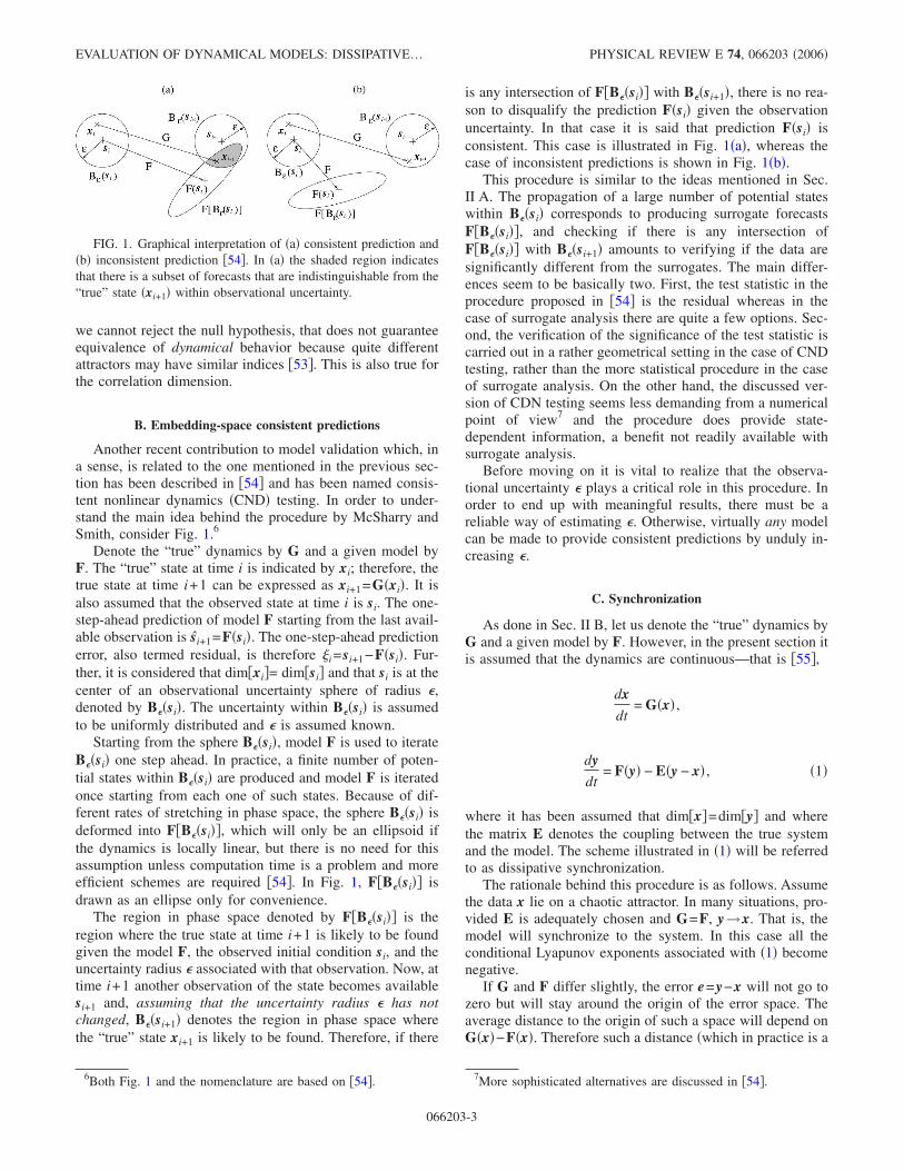
Another recent contribution to model validation which, ina sense, is related to the one mentioned in the previous sec-tion has been described in �54� and has been named consis-tent nonlinear dynamics �CND� testing. In order to under-stand the main idea behind the procedure by McSharry andSmith, consider Fig. 1.6

Denote the “true” dynamics by G and a given model byF. The “true” state at time i is indicated by xi; therefore, thetrue state at time i+1 can be expressed as xi+1=G�xi�. It isalso assumed that the observed state at time i is si. The one-step-ahead prediction of model F starting from the last avail-able observation is si+1=F�si�. The one-step-ahead predictionerror, also termed residual, is therefore �i=si+1−F�si�. Fur-ther, it is considered that dim�xi�= dim�si� and that si is at thecenter of an observational uncertainty sphere of radius �,denoted by B��si�. The uncertainty within B��si� is assumedto be uniformly distributed and � is assumed known.

Starting from the sphere B��si�, model F is used to iterateB��si� one step ahead. In practice, a finite number of poten-tial states within B��si� are produced and model F is iteratedonce starting from each one of such states. Because of dif-ferent rates of stretching in phase space, the sphere B��si� isdeformed into F�B��si��, which will only be an ellipsoid ifthe dynamics is locally linear, but there is no need for thisassumption unless computation time is a problem and moreefficient schemes are required �54�. In Fig. 1, F�B��si�� isdrawn as an ellipse only for convenience.

The region in phase space denoted by F�B��si�� is theregion where the true state at time i+1 is likely to be foundgiven the model F, the observed initial condition si, and theuncertainty radius � associated with that observation. Now, attime i+1 another observation of the state becomes availablesi+1 and, assuming that the uncertainty radius � has notchanged, B��si+1� denotes the region in phase space wherethe “true” state xi+1 is likely to be found. Therefore, if there

is any intersection of F�B��si�� with B��si+1�, there is no rea-son to disqualify the prediction F�si� given the observationuncertainty. In that case it is said that prediction F�si� isconsistent. This case is illustrated in Fig. 1�a�, whereas thecase of inconsistent predictions is shown in Fig. 1�b�.

This procedure is similar to the ideas mentioned in Sec.II A. The propagation of a large number of potential stateswithin B��si� corresponds to producing surrogate forecastsF�B��si��, and checking if there is any intersection ofF�B��si�� with B��si+1� amounts to verifying if the data aresignificantly different from the surrogates. The main differ-ences seem to be basically two. First, the test statistic in theprocedure proposed in �54� is the residual whereas in thecase of surrogate analysis there are quite a few options. Sec-ond, the verification of the significance of the test statistic iscarried out in a rather geometrical setting in the case of CNDtesting, rather than the more statistical procedure in the caseof surrogate analysis. On the other hand, the discussed ver-sion of CDN testing seems less demanding from a numericalpoint of view7 and the procedure does provide state-dependent information, a benefit not readily available withsurrogate analysis.

Before moving on it is vital to realize that the observa-tional uncertainty � plays a critical role in this procedure. Inorder to end up with meaningful results, there must be areliable way of estimating �. Otherwise, virtually any modelcan be made to provide consistent predictions by unduly in-creasing �.

C. Synchronization

As done in Sec. II B, let us denote the “true” dynamics byG and a given model by F. However, in the present section itis assumed that the dynamics are continuous—that is �55�,

dx

dt= G�x� ,

dy

dt= F�y� − E�y − x� , �1�

where it has been assumed that dim�x�=dim�y� and wherethe matrix E denotes the coupling between the true systemand the model. The scheme illustrated in �1� will be referredto as dissipative synchronization.

The rationale behind this procedure is as follows. Assumethe data x lie on a chaotic attractor. In many situations, pro-vided E is adequately chosen and G=F, y→x. That is, themodel will synchronize to the system. In this case all theconditional Lyapunov exponents associated with �1� becomenegative.

If G and F differ slightly, the error e=y−x will not go tozero but will stay around the origin of the error space. Theaverage distance to the origin of such a space will depend onG�x�−F�x�. Therefore such a distance �which in practice is a

6Both Fig. 1 and the nomenclature are based on �54�. 7More sophisticated alternatives are discussed in �54�.

FIG. 1. Graphical interpretation of �a� consistent prediction and�b� inconsistent prediction �54�. In �a� the shaded region indicatesthat there is a subset of forecasts that are indistinguishable from the“true” state �xi+1� within observational uncertainty.

EVALUATION OF DYNAMICAL MODELS: DISSIPATIVE… PHYSICAL REVIEW E 74, 066203 �2006�

066203-3

measure of quality of “synchronization”� is a measure ofhow far the estimated model F is from the true dynamics G�55�.

In order to implement this scheme in practice the authorssuggested taking matrix E to be diagonal with only one ele-ment different from zero. The authors then compare �x−z� —where z is the model state vector without any driving force to�x−y�. If �x−y� drops below a certain threshold �10−2 wasused in �56�� and is “clearly” smaller than �x−z�—that is, x�y—and it is assumed that the model is synchronized to thedata, F should therefore be sufficiently close to G.

As often happens in the realm of model validation, thisprocedure also is highly subjective, since it requires an adhoc threshold, mentioned in the previous paragraph. In whatconcerns dissipative synchronization, it is well known that inmany cases by increasing the strength of the coupling �ma-trix E� it is possible to force a greater degree of synchroni-zation and, in some cases, even attain identical synchroniza-tion �55�. For instance, in �56� the authors found that forvalues of the coupling greater than 2, models of an electroniccircuit would synchronize with the measured data. On theother hand, Letellier et al. �57� have found a lower bound of0.1 for the coupling strength in order to guarantee synchro-nization between the Rössler system and perturbed versionsof the original equations. It therefore becomes clear that it issometimes possible to synchronize even a poor model to thedata as long as the coupling strength is made sufficientlylarge. In fact, is has been shown that even different systemscan synchronize, at a rather high cost �58�.

Therefore although the concept of synchronization couldbe useful in the context of model validation, it becomes ap-parent that some adjustments are required to render the pro-cedure more practical. Some steps in this direction will begiven in the next section. Before, it is noted that synchroni-zation has been used in parameter estimation problems�16,59–61�.

III. DATA-MODEL SYNCHRONIZATIONFOR DISCRETE MODELS

In this section a procedure based on dissipative synchro-nization is proposed in the context of model evaluation.Compared to the first procedure put forward in �55�, thepresent method is different at least in three important aspects.First, the method has been developed for discrete-time mod-els. Second, the criterion for evaluating a model is not if themodel synchronizes �for the reasons discussed above� butrather is the cost of synchronization. Consequently, the syn-chronization scheme used does not seem to be critical sincewe aim at a relative evaluation of models rather than anabsolute one.8 Clearly, if the aim were to optimize synchro-nization, other synchronization schemes would have to beconsidered. It will be argued that better models cost less tosynchronize with the data, with respect to dissipative syn-

chronization. Therefore an index that measures the cost ofmaintaining models synchronized will be used; see Sec.III B. Third, in order to compare the cost of synchronizationin a meaningful way, it is necessary to guarantee that thequality of the synchronization is similar. The following pro-cedure will use the concept of class of synchronization de-fined in �62�; see Sec. III C.

A. Main motivation

It is assumed that the available data are scalar and discretesequences x�k� �output� and u�k� �input�, for k=1,2 , . . . ,N.In the case no input is measured, the procedure remains validwith u�k�=0,∀ k. It is assumed that the data are correctlydescribed by

x�k� = g„�ux�k − 1�… , �2�

where �ux�k−1� is a vector composed of lagged values of thedata x and u up to and possibly including instant k−1. It isnot assumed that the embedding is regular, in the sense of�25�. Finally, g is an unknown function that relates all thevariables in �ux�k−1� to the future output x�k�.

Analogously, it is assumed that a model9 f has been ob-

tained from the given data such that x�k�= f(�ux�k−1�)+��k�, where the deterministic one-step-ahead prediction of

the model is f(�ux�k−1�) and ��k� is an error function. Inprinciple there is no need to assume that ��k� is white or that

is has a certain probability distribution. Here, �ux�k−1� is thevector of model-independent variables. It is not assumed that

�ux�k−1� and �ux�k−1� include the same set of lags.Initially, it is desired to verify if model f will synchronize

with the observed data. To investigate this, the followingdissipative synchronization scheme can be easily imple-mented:

x�k� = g„�ux�k − 1�… ,

y�k� = f„�ux�k − 1�… − h�k − 1� , �3�

where h�k�=c(x�k�− y�k�) and c�R is a constant. It isinteresting to notice that in �3�, besides the dissipative cou-pling term, direct substitution of y with x has taken place. Insuch a framework the one-step-ahead synchronization error�OSASE� is defined as

e�k� = x�k� − y�k� = g„�ux�k − 1�… − �f„�ux�k − 1�… − h�k − 1��

= c„x�k − 1� − y�k − 1�… + �g„�ux�k − 1�… − f„�ux�k − 1�…�

= ce�k − 1� + ��k − 1� . �4�

It is instructive to see that Eq. �4� is fundamentally anARX �autoregressive with an exogenous input� model.Therefore, the OSASE is a first-order autoregressive processdriven by the “exogenous” variable ��k−1�. It is well knownthat in order to have a nondiverging process, �c � �1. More-

8This remark becomes even more important if we consider that insome cases it is possible to synchronize totally different systems�80�.

9No assumptions are made concerning the type of model f apartfrom the fact that it should be a discrete-time model.

AGUIRRE, FURTADO, AND TÔRRES PHYSICAL REVIEW E 74, 066203 �2006�

066203-4

over, whereas the autonomous dynamics is governed by thedissipative coupling �the autoregressive part�, the overall be-havior is determined by the driving function ��k−1� which issimply a measure of the distance between the dynamics un-

derlying the data g(�ux�k−1�) and the model f(�ux�k−1�).Clearly, should the difference between these entities be neg-ligible, ��k−1��0 and e�k� would naturally tend to zero,since �c � �1. Therefore, it is seen that the dynamical mis-

match between g(�ux�k−1�) and f(�ux�k−1�) is somehowreflected in the OSASE e�k�. Therefore e�k� conveys impor-tant dynamical information and, at least in principle, it couldbe used as a measure of model quality. In this particularrespect, the present procedure follows the main motivationin �55�.

B. Cost of synchronization

In many systems synchronization is always possible aslong as the coupling is sufficiently strong �55�. Because ofthis, it seems useless to declare valid a model that is forcedto synchronize with the data. On the other hand, it is a factthat the closer two dynamical systems are, the easier it is tosynchronize them. This last remark is taken to be our greatmotivation to define a measure of the cost of synchronizationthat later will be used to evaluate dynamical models.

The following working definition of cost of synchroniza-tion will be used:

Jrms�c� = limN→�

� 1

N�k=1

N

h�k�2, �5�

where it is assumed that k=1 indicates the instant fromwhich synchronization is achieved and not the first value in

the data sequence. Viewing h�k�=c(x�k�− y�k�) as the controlaction required to maintain the model synchronized to thedata, it is possible to interpret Jrms�c� as the energy requiredto keep the model close to the data. It is stressed that in thepractical computation of Eq. �5� the transients experiencedby the model until it synchronizes with the data �if it everdoes� are not taken into account. This is welcome in practicein so far as the effect of initial conditions is greatly dimin-ished.

It should be noticed that there are many other ways inwhich the coupling �and therefore the cost of synchroniza-tion� can be defined. In particular �63� uses sinusoidal cou-pling and �64� uses sigmoidal coupling. The choice of h�k� inthis paper was made to keep the coupling as simple as pos-sible. In fact, the choice of h�k� is a linear approximation ofthe two nonlinear coupling schemes used in �63,64�. It is ofparamount importance to remember that the aim in this workis not to achieve high-quality synchronization but rather toapply the same synchronization scheme to several systemsand decide which synchronizes with similar quality at alower cost. The following section will shed some light ontohow to assess and quantify synchronization quality.

C. Class of synchronization

In order to compare cost of synchronization in a meaning-ful way, it will be necessary to guarantee that the quality ofthe synchronization is of a certain type. To this end, theconcept of class of synchronization defined in �62� isadapted.

Two synchronized systems will belong to the � class ofsynchronization if and only if

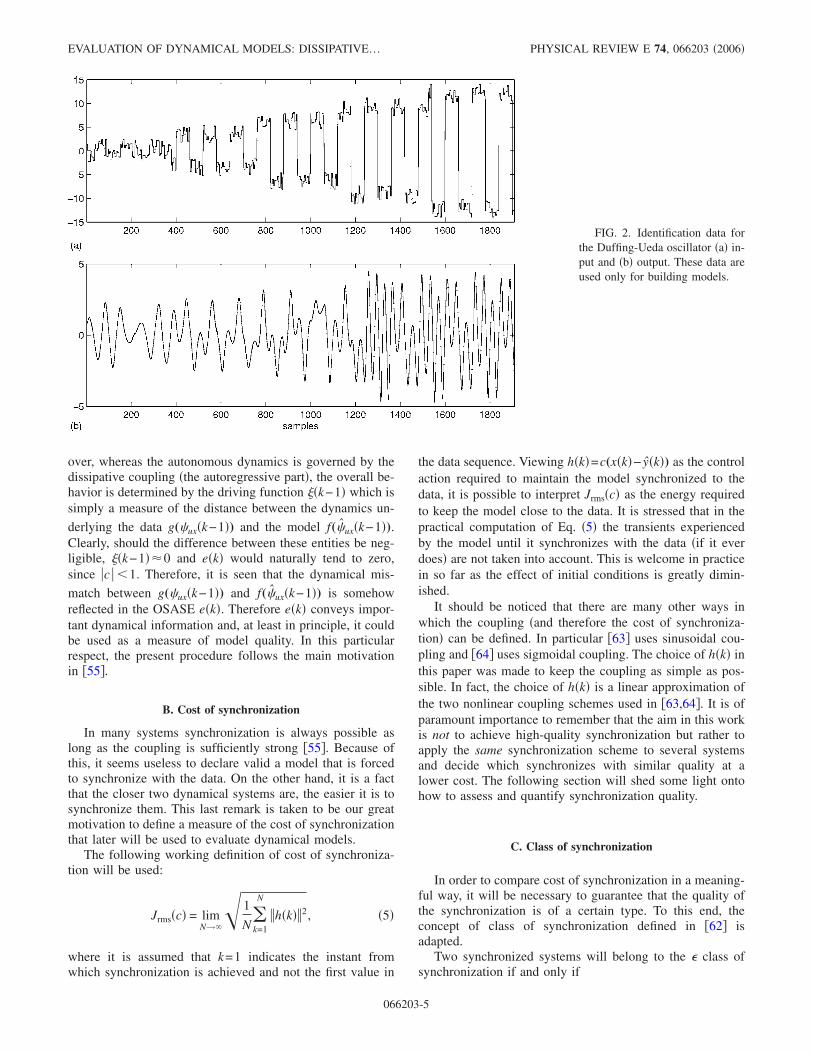
FIG. 2. Identification data forthe Duffing-Ueda oscillator �a� in-put and �b� output. These data areused only for building models.

EVALUATION OF DYNAMICAL MODELS: DISSIPATIVE… PHYSICAL REVIEW E 74, 066203 �2006�

066203-5

supe�k�supe�k� + 1

� ��c�, ∀ k � 1, �6�

where e�k� was defined in Eq. �4� and the dependence of thesynchronization on the linear feedback gain c has been madeexplicit. It is clear that 0���c��1 and that ��c��0 impliesx�k�= y�k� for that particular value of c. On the other hand,��c��1 points to asynchronous behavior. For practical rea-sons, given a particular experiment for which a sequence ofsynchronization errors e�k� is available, it is useful to con-sider the maximum normalized synchronization error, de-fined as

maxe�k�maxe�k� + 1

= �m�c�, ∀ k � 1. �7�

D. Comparing models

The procedure now being presented, as for most valida-tion procedures, also has a certain degree of subjectivity.In view of this, rather than artificially trying to declare acertain model valid or not, the problem to be dealt with is tochoose what seems to be the best model within a set ofcandidates. This has been referred to rather informally asmodel evaluation rather than model validation. The latterseems to suggest an “absolute” quality to the model, and it isarguable if that would be the best way of addressing thewhole matter.

In comparing models, the two concepts presented inSecs. III B and III C, are important. Given two models thatsynchronize with the data in a similar way10 the model withthe “best dynamics” will typically be the one for whichsynchronization can be maintained at a lower cost. Becauseonly one synchronization scheme �dissipative� is imple-mented, it could turn out that assessing models with anotherscheme would rank such a model in a different order. Thoughthis could turn out to be true, it seems that it is not likely.Femat and coworkers, in a different setting, have varied theintensity �gain� of synchronization as well as model mis-match while computing a given performance index. Forevery synchronization case considered, models with lessmismatch could always be recognized without ambiguity�there are no crossings in the performance plots; see theirFig. 4� �65�.

The suggested approach to the problem is as follows.Suppose it is desired to choose among two models M1 andM2 the one with dynamics “closer to the dynamics underly-ing the data.” First of all, the smallest maximum normalizedsynchronization error for each model is determined; that is,we search for �m

1 �c1�=min��m1 �c�� and �m

2 �c2�=min��m2 �c��,

where the minimization is carried out over the range 0�c�1. If the found values are quite different, the models can beranked without further computations. However, if �m

1 �c1���m

2 �c2�, then the criterion to rank the models becomes the

10In this case we shall speak of two models that belong to thesame class of synchronization or that have comparable maximumnormalized synchronization errors.

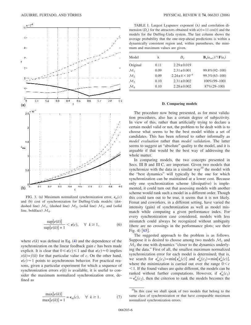
TABLE I. Largest Lyapunov exponent �� and correlation di-mension �Dc� for the attractors obtained with u�t�=11 cos�t� and themodels for the Duffing-Ueda system. The last column shows theaverage probability that the one-step-ahead predictions is within adynamically consistent region and, within parentheses, the mini-mum and maximum values are given.

Model Dc B��si+1��F�si�

Original 0.11 2.29±0.019

M1 0.09 2.31±0.001 99.8%�92–100�M2 0.09 2.24±410−4 99.3%�63–100�M3 0.10 2.31±0.002 100%�99–100�M4 0.10 2.28±0.002 87%�29–100�

FIG. 3. �a� Maximum normalized synchronization error, �m�c�and �b� cost of synchronization for Duffing-Ueda models: �dot-dashed line� M1, �dashed line� M2, �solid line� M3, and �solidline, boldface� M4.

AGUIRRE, FURTADO, AND TÔRRES PHYSICAL REVIEW E 74, 066203 �2006�

066203-6

cost required to maintain models M1 and M2 at �m1 �c1�

��m2 �c2�—that is, Jrms

1 �c1� and Jrms2 �c2�, respectively. The

model that achieves the smallest maximum normalized syn-chronization error at the lowest cost is likely to have betteroverall dynamics, as illustrated in the next section.

IV. NUMERICAL RESULTS

This section presents numerical examples that use well-known nonlinear oscillators.11 As pointed out by Gilmoreand Lefranc, the Duffing and van der Pol oscillators areamong the basic testbeds used in the study of dynamicalsystems theory �66�. Also, the well-known Hénon map �67�will be used. In order to assess the effectiveness of the pro--

cedure put forward in Sec. III various aspects of the originalsystems and of the models will be compared.

A. Duffing oscillator

In the present section, two different versions of theDuffing oscillator will be investigated: the Duffing-Ueda os-cillator �68� and the Duffing-Holmes oscillator �69�. The mo-tivation for investigating both versions is simply that bothversions of the Duffing oscillator have received attention inthe literature. In addition to that, over the parameter rangeinvestigated in this paper, both versions present quite differ-ent behaviors.

1. Ueda equation

The Ueda version of the Duffing oscillator is �68�

y + ky + y3 = u�t� . �8�11The data and code used are available from the authors on

request.

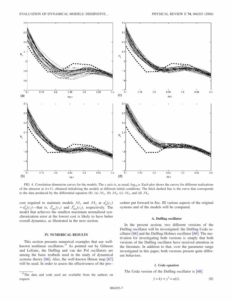
FIG. 4. Correlation dimension curves for the models. The x axis is, as usual, log10 �. Each plot shows the curves for different realizationsof the attractor at A=11, obtained initializing the models at different initial conditions. The thick dashed line is the curve that correspondsto the data produced by the differential equation �8�: �a� M1, �b� M2, �c� M3, and �d� M4.

EVALUATION OF DYNAMICAL MODELS: DISSIPATIVE… PHYSICAL REVIEW E 74, 066203 �2006�

066203-7

In this example, k=0.1. Equation �8� was simulatedwith the input u�t� shown in Fig. 2�a�, thusyielding the output shown in Fig. 2�b�. Numericalin-tegration was carried out using a fourth-order

Runge-Kutta algorithm with integration interval of� /3000. Subsequently the data were sampled atTs=� /60 and used to obtain four models: M1, M2, M3,and M4.

FIG. 5. Bifurcation diagrams with u�t�=A cos�t� and 4.5�A�12 for �a� M1, �b� M2, �c� M3, �d� M4, and �e� original equation �8�. M4

seems to be the best model in what concerns the sequence of bifurcations.

AGUIRRE, FURTADO, AND TÔRRES PHYSICAL REVIEW E 74, 066203 �2006�

066203-8

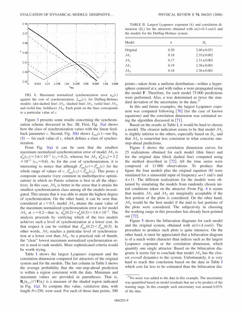
Figure 3 presents some results concerning the synchroni-zation scheme discussed in Sec. III. First, Fig. 3�a� showshow the class of synchronization varies with the linear feed-back parameter c. Second, Fig. 3�b� shows Jrms�c�—see Eq.�5� — for each value of c, which defines a class of synchro-nization.

From Fig. 3�a� it can be seen that the smallestmaximum normalized synchronization error of model M3 is�m

3 �c3��3.610−3 �c3�0.2�, whereas for M4 �m4 �c4��3.2

10−3 �c4�0.6�. As for the cost of synchronization, it isinteresting to notice that although Jrms

3 �c��Jrms4 �c� for the

whole range of values of c, Jrms3 �c3��Jrms

4 �c4�. This poses acomposite scenario �very common in multiobjective optimi-zation� in which no Pareto solution is best in all the objec-tives. In this case, M4 is better in the sense that it attains thesmallest synchronization class among all the models investi-gated. This means that it was able to attain the highest degreeof synchronization. On the other hand, it can be seen that,considered at c�0.5, model M4 attains the same value ofthe maximum normalized synchronization error as for modelM3 at c�0.2—that is, �m

3 �0.2���m4 �0.5��3.610−3. The

analysis proceeds by verifying which of the two modelsachieves such a level of synchronization at a lower cost. Inthat respect it can be verified that Jrms

3 �0.2��Jrms4 �0.5�. In

other words, M3 reaches a particular level of synchroniza-tion at a lower cost than M4. As a practical rule of thumb,the “clear” lowest maximum normalized synchronization er-ror is used to rank models. More sophisticated criteria wouldbe worth trying.

Table I shows the largest Lyapunov exponent and thecorrelation dimension computed for attractors of the originalsystem and for the models. The last column in Table I showsthe average probability that the one-step-ahead predictionis within a region consistent with the data. Minimum andmaximum values are provided in parentheses. That is,B��si+1��F�si� is a measure of the shaded region indicatedin Fig. 1�a�. To compute this value, validation data, withlength N=250, were used. For each of those data points, 300

points—taken from a uniform distribution—within a hyper-sphere centered at si and with radius � were propagated usingthe model F. Therefore, for each model 75 000 predictionswere performed. Also, � was determined as twice the stan-dard deviation of the uncertainty in the data.12

In this and future examples, the largest Lyapunov expo-nent was computed following �70� �for the case of knownequations� and the correlation dimension was estimated us-ing the algorithm discussed in �71�.

Based on the results in Table I, it would be hard to choosea model. The clearest indication seems to be that model M2is slightly inferior to the others, especially based on Dc, andthat M4 is somewhat less consistent in what concerns one-step-ahead predictions.

Figure 4 shows the correlation dimension curves for25 realizations obtained for each model �thin lines� andfor the original data �thick dashed line� computed usingthe method described in �72�. All the time series werecomposed of 11 000 observations. To produce thatfigure the four models plus the original equation �8� weresimulated for a sinusoidal input of frequency �=1 rad/s andA=11. The different realizations for the models were ob-tained by simulating the models from randomly chosen ini-tial conditions taken on the attractor. From Fig. 4 it seemsthat models M1 and M2 are marginally acceptable if thefirst portion of the plots is considered. On the other hand,M4 would be the best model if the mid to last portions ofthe plots were considered. The subjectivity in choosingthe working range in this procedure has already been pointedout �72�.

Figure 5 shows the bifurcation diagrams for each modeland the original system, obtained with u�t�=A cos�t�. Theprocedure to produce such plots is quite intensive. On theother hand, it must be appreciated that a bifurcation diagramis of a much wider character than indices such as the largestLyapunov exponent or the correlation dimension, whichquantify one single attractor. Based on the bifurcation dia-grams it seems fair to conclude that model M4 has the clos-est overall dynamics to the system. Unfortunately, it is veryhard to reach this conclusion based on the data in Table Iwhich cost far less to be estimated than the bifurcation dia-

12No noise was added to the data in this example. The uncertaintywas quantified based on model residuals that are a by-product of thetraining stage. In this example such uncertainty was around 0.03%of the data.

TABLE II. Largest Lyapunov exponent �� and correlation di-mension �Dc� for the attractors obtained with u�t�=0.3 cos�t� andthe models for the Duffing-Holmes system.

Model Dc

Original 0.20 2.40±0.021

M1 0.18 2.35±0.002

M2 0.17 2.31±0.002

M3 0.19 2.38±0.001

M4 0.18 2.36±0.001

FIG. 6. Maximum normalized synchronization error �m�c�against the cost of synchronization, Jrms�c�, for Duffing-Holmesmodels: �dot-dashed line� M1, �dashed line� M2, �solid line� M3,and �solid line, boldface� M4. Each point on the lines correspondsto a particular value of c.

EVALUATION OF DYNAMICAL MODELS: DISSIPATIVE… PHYSICAL REVIEW E 74, 066203 �2006�

066203-9

grams. Moreover, it is not always feasible to produce suchdiagrams for real systems.

Therefore, based on the proposed synchronization schemeand many other criteria, it seems adequate to state that mod-els M3 and M4 are clearly superior to M1 and M2 in

overall terms, and although M3 is quite competitive, M4seems best overall.

As pointed out in Sec. III A, the model class of f isnot taken into account in any part of the analysis. Inthe present and following examples the models used

FIG. 7. Bifurcation diagrams with u�t�=A cos�t� and 0.22�A�0.35 for �a� M1, �b� M2, �c� M3, �d� M4, and �e� original equation �9�.Based on this figure, M3 seems to be the best model.

AGUIRRE, FURTADO, AND TÔRRES PHYSICAL REVIEW E 74, 066203 �2006�

066203-10

were nonlinear discrete-time polynomials. As a part ofthis first example, however, two additional neural-networkmultilayer perceptron models were considered.13 Onemodel was known to reproduce fairly well the originaldynamics of the Duffing-Ueda oscillator whereas the otherone not �6�. Following the procedure described in thispaper the best network model did achieve a much lowermaximum normalized synchronization error at a muchsmaller cost than the network with poor dynamical perfor-mance, thus confirming the scenario observed for modelsM1, M2, M3, and M4. Finally, it is mentioned thatin �49� a continuous-time nonlinear polynomial modelwas obtained and made to synchronize by dissipativecoupling. The authors validated such a model by means oftopological analysis and suggested that the model topologicalvalidity was consistent with the fact that it was possible tosynchronize it to the data. The fact that three different modelclasses showed consistency between synchronization andvalidation results suggests that the proposed procedure is, infact, somewhat robust to the model class.

Before moving on, it is pointed out that in view of theresults discussed in this example, in the next examples theCND testing and the correlation curves will be omitted andonly nonlinear polynomial models will be considered.

2. Holmes equation

The Duffing-Holmes system is �69�

y + y − �y + y3 = A cos��t� . �9�

As before, data were obtained by numerically integratingEq. �9� with =0.15, �=1, A=0.3, and �=1 rad/s, forwhich the system settles to a chaotic attractor. Data sampledat Ts=� /15 were used to obtain four models: M1, M2, M3,and M4.

The synchronization procedure discussed in Sec. IIIyielded the results summarized in Fig. 6. That figure showsthe maximum normalized synchronization error �i.e., the es-timated class of synchronization� against the cost of synchro-nization. Each point on the lines in that figure corresponds toa particular value of c. From Fig. 6 it is seen that althoughmin��m

4 �c�� is slightly smaller than min��m3 �c��, the cost of

synchronizing M3 is significantly smaller than that of syn-chronizing M4. Therefore, Fig. 6 suggests that M3 is supe-

rior to M4, because it was possible to find a value of cou-pling such that the cost to synchronize M3 to the data with acertain quality is smaller than for M4 �and the other mod-els�. Another feature illustrated in that figure, is that M2 issimilar to M3 in what concerns synchronization and the costto maintain it.

The largest Lyapunov exponent and the correlation di-mension of the models are shown in Table II. In view of theresults for the Duffing-Ueda oscillator CND testing was notperformed in the present example or in the next. From thedata in the table, it seems that model M2 is slightly worsethan the others. It is apparent that results such as those illus-trated in Table II lack discrimination power.

The bifurcation diagrams shown in Fig. 7 suggest thatM2 and M3 are the best, with M3 being somewhat superior.M1 and M4 have many spurious chaotic windows. All themodels have a narrow periodic window which appears in theoriginal system just before A�0.32. In the case of M1 andM4 such a window appears just after A�0.32. Models M2and M3 present such a window just before A�0.32, as forthe original system. M2, however, still presents a spuriouschaotic window for A�0.32.

It is remarkable that, unlike for the Duffing-Ueda system,in the case of the Duffing-Holmes system �and also for thevan der Pol oscillator as will be seen later� the input was asingle-frequency signal and therefore the output, based onwhich the models were obtained, was on a single attractor.Nevertheless, such data do convey a great deal of informa-tion concerning how the original system bifurcates. In otherwords, although the model-building data were located at asingle value of A in the bifurcation diagram, a rather widerange of values was successfully covered by the models.

B. van der Pol oscillator

This example considers the modified van der Pol oscilla-tor �73�

y + ��y2 − 1�y + y3 = u�t� . �10�13We thank Dr. Gleison Amaral for providing such models. See

�6� for the details.

TABLE III. Largest Lyapunov exponent �� and correlation di-mension �Dc� for the attractors obtained with u�t�=17 cos�4t� andthe models for the van der Pol oscillator.

Model Dc

Original 0.33 2.44±0.001

M1 0.32 2.46±0.003

M2 0.34 2.53±0.001

M3 0.31 2.41±0.012

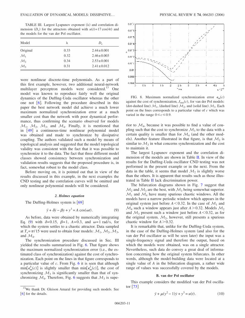
FIG. 8. Maximum normalized synchronization error �m�c�against the cost of synchronization, Jrms�c�, for van der Pol models:�dot-dashed line� M1, �dashed line� M2, and �solid line� M3. Eachpoint on the lines corresponds to a particular value of c which wasvaried in the range 0�c�0.9.

EVALUATION OF DYNAMICAL MODELS: DISSIPATIVE… PHYSICAL REVIEW E 74, 066203 �2006�

066203-11

Equation �10� was integrated with �=0.2, u�t�=A cos��t�,A=17, and �=4 rad/s, which yields a chaotic attractor.Data sampled at Ts=� /80 were used to obtain three models,M1, M2, and M3, for which the information on synchroni-zation class and cost is summarized in Fig. 8. Such resultssuggest that M3 is probably the best overall model because,although the cost of synchronization is roughly the same forthe three models �it is slightly smaller for M3�, the maxi-mum normalized synchronization error is significantlysmaller for M3.

The largest Lyapunov exponent and the correlation di-mension of models M1, M2, and M3 are shown in TableIII. From the data in the table, it seems that model M1 isclosest to the original system, with M3 being also quite goodand M2 being the poorest model.

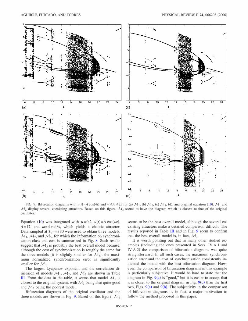
Bifurcation diagrams of the original oscillator and thethree models are shown in Fig. 9. Based on this figure, M3

seems to be the best overall model, although the several co-existing attractors make a detailed comparison difficult. Theresults reported in Table III and in Fig. 9 seem to confirmthat the best overall model is, in fact, M3.

It is worth pointing out that in many other studied ex-amples �including the ones presented in Secs. IV A 1 andIV A 2� the comparison of bifurcation diagrams was quitestraightforward. In all such cases, the maximum synchroni-zation error and the cost of synchronization consistently in-dicated the model with the best bifurcation diagram. How-ever, the comparison of bifurcation diagrams in this exampleis particularly subjective. It would be hard to state that thediagram in Fig. 9�c� is “good,” but it is easier to accept thatit is closer to the original diagram in Fig. 9�d� than the firsttwo, Figs. 9�a� and 9�b�. The subjectivity in the comparisonof bifurcation diagrams is, in fact, a major motivation tofollow the method proposed in this paper.

FIG. 9. Bifurcation diagrams with u�t�=A cos�4t� and 4�A�25 for �a� M1, �b� M2, �c� M3, �d�, and original equation �10�. M1 andM2 display several coexisting attractors. Based on this figure, M3 seems to have the diagram which is closest to that of the originaloscillator.

AGUIRRE, FURTADO, AND TÔRRES PHYSICAL REVIEW E 74, 066203 �2006�

066203-12

C. Hénon map

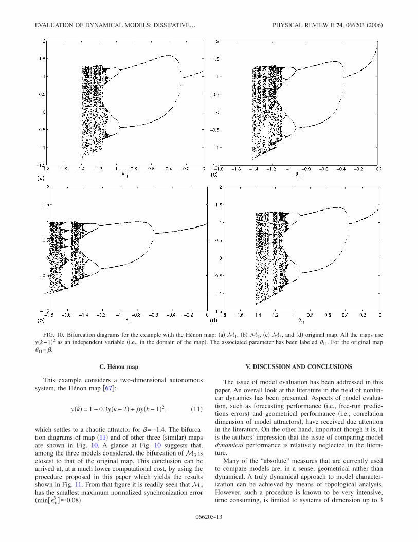
This example considers a two-dimensional autonomoussystem, the Hénon map �67�:

y�k� = 1 + 0.3y�k − 2� + �y�k − 1�2, �11�

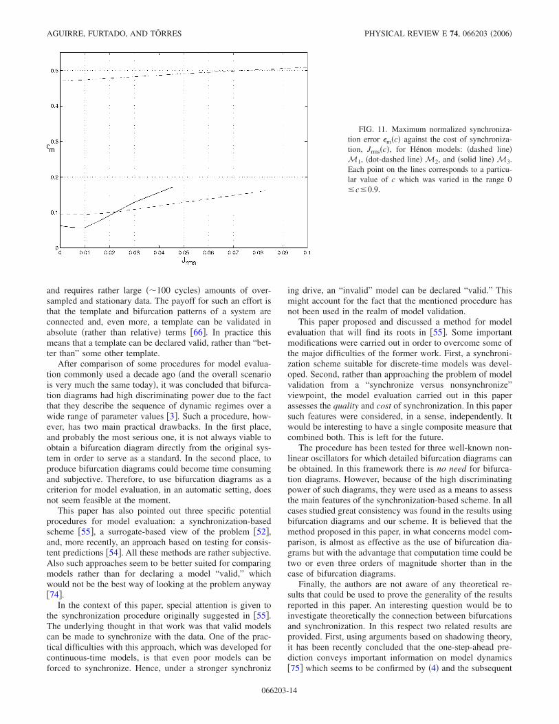
which settles to a chaotic attractor for �=−1.4. The bifurca-tion diagrams of map �11� and of other three �similar� mapsare shown in Fig. 10. A glance at Fig. 10 suggests that,among the three models considered, the bifurcation of M3 isclosest to that of the original map. This conclusion can bearrived at, at a much lower computational cost, by using theprocedure proposed in this paper which yields the resultsshown in Fig. 11. From that figure it is readily seen that M3has the smallest maximum normalized synchronization error�min��m

3 ��0.08�.

V. DISCUSSION AND CONCLUSIONS

The issue of model evaluation has been addressed in thispaper. An overall look at the literature in the field of nonlin-ear dynamics has been presented. Aspects of model evalua-tion, such as forecasting performance �i.e., free-run predic-tions errors� and geometrical performance �i.e., correlationdimension of model attractors�, have received due attentionin the literature. On the other hand, important though it is, itis the authors’ impression that the issue of comparing modeldynamical performance is relatively neglected in the litera-ture.

Many of the “absolute” measures that are currently usedto compare models are, in a sense, geometrical rather thandynamical. A truly dynamical approach to model character-ization can be achieved by means of topological analysis.However, such a procedure is known to be very intensive,time consuming, is limited to systems of dimension up to 3

FIG. 10. Bifurcation diagrams for the example with the Hénon map: �a� M1, �b� M2, �c� M3, and �d� original map. All the maps usey�k−1�2 as an independent variable �i.e., in the domain of the map�. The associated parameter has been labeled �11. For the original map�11=�.

EVALUATION OF DYNAMICAL MODELS: DISSIPATIVE… PHYSICAL REVIEW E 74, 066203 �2006�

066203-13

and requires rather large �100 cycles� amounts of over-sampled and stationary data. The payoff for such an effort isthat the template and bifurcation patterns of a system areconnected and, even more, a template can be validated inabsolute �rather than relative� terms �66�. In practice thismeans that a template can be declared valid, rather than “bet-ter than” some other template.

After comparison of some procedures for model evalua-tion commonly used a decade ago �and the overall scenariois very much the same today�, it was concluded that bifurca-tion diagrams had high discriminating power due to the factthat they describe the sequence of dynamic regimes over awide range of parameter values �3�. Such a procedure, how-ever, has two main practical drawbacks. In the first place,and probably the most serious one, it is not always viable toobtain a bifurcation diagram directly from the original sys-tem in order to serve as a standard. In the second place, toproduce bifurcation diagrams could become time consumingand subjective. Therefore, to use bifurcation diagrams as acriterion for model evaluation, in an automatic setting, doesnot seem feasible at the moment.

This paper has also pointed out three specific potentialprocedures for model evaluation: a synchronization-basedscheme �55�, a surrogate-based view of the problem �52�,and, more recently, an approach based on testing for consis-tent predictions �54�. All these methods are rather subjective.Also such approaches seem to be better suited for comparingmodels rather than for declaring a model “valid,” whichwould not be the best way of looking at the problem anyway�74�.

In the context of this paper, special attention is given tothe synchronization procedure originally suggested in �55�.The underlying thought in that work was that valid modelscan be made to synchronize with the data. One of the prac-tical difficulties with this approach, which was developed forcontinuous-time models, is that even poor models can beforced to synchronize. Hence, under a stronger synchroniz

ing drive, an “invalid” model can be declared “valid.” Thismight account for the fact that the mentioned procedure hasnot been used in the realm of model validation.

This paper proposed and discussed a method for modelevaluation that will find its roots in �55�. Some importantmodifications were carried out in order to overcome some ofthe major difficulties of the former work. First, a synchroni-zation scheme suitable for discrete-time models was devel-oped. Second, rather than approaching the problem of modelvalidation from a “synchronize versus nonsynchronize”viewpoint, the model evaluation carried out in this paperassesses the quality and cost of synchronization. In this papersuch features were considered, in a sense, independently. Itwould be interesting to have a single composite measure thatcombined both. This is left for the future.

The procedure has been tested for three well-known non-linear oscillators for which detailed bifurcation diagrams canbe obtained. In this framework there is no need for bifurca-tion diagrams. However, because of the high discriminatingpower of such diagrams, they were used as a means to assessthe main features of the synchronization-based scheme. In allcases studied great consistency was found in the results usingbifurcation diagrams and our scheme. It is believed that themethod proposed in this paper, in what concerns model com-parison, is almost as effective as the use of bifurcation dia-grams but with the advantage that computation time could betwo or even three orders of magnitude shorter than in thecase of bifurcation diagrams.

Finally, the authors are not aware of any theoretical re-sults that could be used to prove the generality of the resultsreported in this paper. An interesting question would be toinvestigate theoretically the connection between bifurcationsand synchronization. In this respect two related results areprovided. First, using arguments based on shadowing theory,it has been recently concluded that the one-step-ahead pre-diction conveys important information on model dynamics�75� which seems to be confirmed by �4� and the subsequent

FIG. 11. Maximum normalized synchroniza-tion error �m�c� against the cost of synchroniza-tion, Jrms�c�, for Hénon models: �dashed line�M1, �dot-dashed line� M2, and �solid line� M3.Each point on the lines corresponds to a particu-lar value of c which was varied in the range 0�c�0.9.

AGUIRRE, FURTADO, AND TÔRRES PHYSICAL REVIEW E 74, 066203 �2006�

066203-14

discussion. Second, for continuous-time models, it has beenshown that the control action needed to achieve identicalsynchronization equals the vector field mismatch betweenthe two considered systems �62�. Such a result has been re-cently extended to discrete-time systems, and it has beenshown that the synchronization effort is a measure of thedynamical structural mismatch between the two consideredsystems �76�. In any case, such considerations should only be

regarded as starting points for a more precise and theoreticalanalysis of the procedure presented in this paper.

ACKNOWLEDGMENTS

The authors are grateful to Christophe Letellier for a criti-cal reading of the manuscript. Financial support from CNPqis gratefully acknowledged.

�1� J. P. Crutchfield and B. S. McNamara, Complex Syst. 1, 417�1987�.

�2� P. E. Rapp, T. I. Schmah, and A. I. Mees, Physica D 132, 133�1999�.

�3� L. A. Aguirre and S. A. Billings, Int. J. Bifurcation ChaosAppl. Sci. Eng. 4, 109 �1994�.

�4� Y. V. Kolokolov and A. V. Monovskaya, Int. J. BifurcationChaos Appl. Sci. Eng. 16, 85 �2006�.

�5� T. P. Lim and Puthusserypady, Chaos 16, 013106 �2006�.�6� L. A. Aguirre, R. A. M. Lopes, G. Amaral, and C. Letellier,

Phys. Rev. E 69, 026701 �2004�.�7� L. A. Aguirre and E. M. Mendes, Int. J. Bifurcation Chaos

Appl. Sci. Eng. 6, 279 �1996�.�8� E. Bagarinao, K. Pakdaman, T. Nomura, and S. Sato, Phys.

Rev. E 60, 1073 �1999�.�9� E. Bagarinao, K. Pakdaman, T. Nomura, and S. Sato, Physica

D 130, 211 �1999�.�10� S. A. Billings and D. Coca, Int. J. Bifurcation Chaos Appl. Sci.

Eng. 9, 1263 �1999�.�11� J. H. B. Deane, Electron. Lett. 29, 957 �1993�.�12� D. C. Hamil �unpublished�.�13� H. M. Henrique, E. L. Lima, and J. C. Pinto, Lat. Am. Appl.

Res. 28, 187 �1998�.�14� L. Le Sceller, C. Letellier, and G. Gouesbet, Phys. Lett. A 211,

211 �1996�.�15� S. Ogawa, T. Ikeguuchi, T. Matozaki, and K. Aihara, IEICE

Trans. Fundamentals E79-A, 1608 �1996�.�16� C. Tao, Y. Zhang, G. Du, and J. J. Jiang, Phys. Lett. A 332,

197 �2004�.�17� R. Bakker, J. C. Schouten, C. L. Giles, F. Takens, and C. M.

van den Bleek, Neural Comput. 12, 2355 �2000�.�18� M. Small and C. K. Tse, Phys. Rev. E 66, 066701 �2002�.�19� E. Bagarinao and S. Sato, Ann. Biomed. Eng. 30, 260 �2002�.�20� B. P. Bezruchko and D. A. Smirnov, Phys. Rev. E 63, 016207

�2001�.�21� A. Garulli, C. Mocenni, A. Vicino, and A. Tesi, Int. J. Bifur-

cation Chaos Appl. Sci. Eng. 13, 357 �2003�.�22� G. Gouesbet and C. Letellier, Phys. Rev. E 49, 4955 �1994�.�23� H. L. Hiew and C. P. Tsang, Inf. Sci. �N.Y.� 81, 193 �1994�.�24� L. Jaeger and H. Kantz, Chaos 6, 440 �1996�.�25� K. Judd and A. I. Mees, Physica D 120, 273 �1998�.�26� C. Letellier, L. Le Sceller, G. Gouesbet, F. Lusseyran, A. Ke-

moun, and B. Izrar, AIChE J. 43, 2194 �1997�.�27� U. Parlitz et al., Chaos 14, 420 �2004�.�28� P. Perona, A. Porporato, and L. Ridolfi, Nonlinear Dyn. 23, 13

�2000�.�29� B. Pilgram, K. Judd, and A. I. Mees, Physica D 170, 103

�2002�.�30� K. Rodríguez-Vázquez and P. J. Fleming, Knowledge Inf. Syst.

8, 235 �2005�.�31� J. Timmer, Int. J. Bifurcation Chaos Appl. Sci. Eng. 8, 1505

�1998�.�32� J. Timmer, H. Rust, W. Horbelt, and H. U. Voss, Phys. Lett. A

274, 123 �2000�.�33� L. M. Pecora, T. L. Carroll, and J. F. Heagy, Phys. Rev. E 52,

3420 �1995�.�34� K. H. Chon, J. K. Kanters, R. J. Cohen, and N. H. Holstein-

Rathlou, Physica D 99, 471 �1997�.�35� D. Coca and S. A. Billings, Phys. Lett. A 287, 65 �2001�.�36� S. Ishii and M. A. Sato, Neural Networks 14, 1239 �2001�.�37� E. M. A. M. Mendes and S. A. Billings, Int. J. Bifurcation

Chaos Appl. Sci. Eng. 7, 2593 �1997�.�38� E. M. A. M. Mendes and S. A. Billings, IEEE Trans. Man

Cybernet.: Part A 36, 597 �2001�.�39� L. A. Aguirre and S. A. Billings, Int. J. Bifurcation Chaos

Appl. Sci. Eng. 5, 449 �1995�.�40� D. Allingham, M. West, and A. I. Mees, Int. J. Bifurcation

Chaos Appl. Sci. Eng. 8, 2191 �1998�.�41� B. P. Bezruchko, A. S. Karavaev, V. I. Ponomarenko, and M.

D. Prokhorov, Phys. Rev. E 64, 056216 �2001�.�42� G. Boudjema and B. Cazelles, Chaos, Solitons Fractals 12,

2051 �2001�.�43� R. Brown, V. In, and E. R. Tracy, Physica D 102, 208 �1997�.�44� C. S. M. Lainscsek, C. Letellier, and F. Schürrer, Phys. Rev. E

64, 016206 �2001�.�45� J. Maquet, C. Letellier, and L. A. Aguirre, J. Theor. Biol. 228,

421 �2004�.�46� O. Ménard, C. Letellier, J. Maquet, L. Le Sceller, and G.

Gouesbet, Int. J. Bifurcation Chaos Appl. Sci. Eng. 10, 1759�2000�.

�47� C. Letellier and G. Gouesbet, J. Phys. II 6, 1615 �1996�.�48� C. Letellier, L. Le Sceller, P. Dutertre, G. Gouesbet, Z. Fei,

and J. L. Hudson, J. Phys. Chem. A99, 7016 �1995�.�49� N. B. Tufillaro, P. Wyckoff, R. Brown, T. Schreiber, and T.

Molteno, Phys. Rev. E 51, 164 �1995�.�50� J. Theiler, S. Eubank, A. Longtin, B. Galdrijian, and J. D.

Farmer, Physica D 58, 77 �1992�.�51� J. Timmer, Phys. Rev. E 58, 5153 �1998�.�52� M. Small and K. Judd, Physica D 117, 283 �1998�.�53� C. Letellier, T. D. Tsankov, G. Byrne, and R. Gilmore, Phys.

Rev. E 72, 026212 �2005�.�54� P. E. McSharry and L. A. Smith, Physica D 192, 1 �2004�.�55� R. Brown, N. F. Rul’kov, and E. R. Tracy, Phys. Rev. E 49,

3784 �1994�.

EVALUATION OF DYNAMICAL MODELS: DISSIPATIVE… PHYSICAL REVIEW E 74, 066203 �2006�

066203-15

�56� R. Brown, N. F. Rulkov, and E. R. Tracy, Phys. Lett. A 194,71 �1994�.

�57� C. Letellier, O. Ménard, and L. A. Aguirre, in Modeling andForecasting Financial Data: Techniques of Nonlinear Dynam-ics, edited by A. S. Soofi and L. Cao �Kluwer, Dordrecht,2002�, pp. 283–302.

�58� C. Sarasola, F. J. Torrrealdea, A. dAnjou, and M. Graña, Math.Comput. Simul. 58, 309 �2002�.

�59� U. S. Freitas, E. E. N. Macau, and C. Grebogi, Phys. Rev. E71, 047203 �2005�.

�60� A. Maybhate and R. E. Amritkar, Phys. Rev. E 59, 284 �1999�.�61� U. Parlitz, Phys. Rev. Lett. 76, 1232 �1996�.�62� L. A. B. Tôrres and L. A. Aguirre, Physica D 196, 387 �2004�.�63� L. H. A. Monteiro, N. C. F. Canto, J. G. Chaui-Berlinck, F. M.

Orsatti, and J. R. C. Piqueira, IEEE Trans. Neural Netw. 14,1572 �2003�.

�64� L. H. A. Monteiro, M. A. Bussab, and J. G. Chaui-Berlinck, J.Theor. Biol. 219, 83 �2002�.

�65� R. Femat, R. Jauregui-Ortiz, and G. Solis-Perales, IEEE Trans.Circuits Syst., I: Fundam. Theory Appl. 48, 1161 �2001�.

�66� R. Gilmore and M. Lefranc, The Topology of Chaos �WileyInterscience, New York, 2002�.

�67� M. Hénon, Commun. Math. Phys. 50, 69 �1976�.�68� Y. Ueda, Int. J. Non-Linear Mech. 20, 481 �1985�.�69� P. J. Holmes, Philos. Trans. R. Soc. London, Ser. A 292, 419

�1979�.�70� A. Wolf, J. B. Swift, H. L. Swinney, and J. A. Vastano, Physica

D 16, 285 �1985�.�71� D. Yu, M. Small, R. G. Harrison, and C. Diks, Phys. Rev. E

61, 3750 �2000�.�72� K. Judd, Physica D 56, 216 �1992�.�73� Y. Ueda and N. Akamatsu, IEEE Trans. Circuits Syst. 28, 217

�1981�.�74� K. Judd, in Chaos and Its Reconstruction, edited by G. Goues-

bet, S. Meunier-Guttin-Cluzel, and O. Ménard �Nova Science,New York, 2003�, pp. 179–214.

�75� D. Orrell, Int. J. Bifurcation Chaos Appl. Sci. Eng. 15, 3265�2005�.

�76� L. A. B. Tôrres �unpublished�.�77� M. Small, D. Yu, and R. G. Harrison, Int. J. Bifurcation Chaos

Appl. Sci. Eng. 13, 743 �2003�.�78� G. Gouesbet, S. Meunier-Guttin-Cluzel, and O. Ménard, in

Chaos and Its Reconstruction, edited by G. Gouesbet, S.Meunier-Guttin-Cluzel, and O. Ménard �Nova Science, NewYork, 2003�, pp. 1–160.

�79� L. A. Aguirre and A. V. P. Souza, Comput. Biol. Med. 34, 241�2004�.

�80� R. Femat and G. Solis-Perales, Phys. Rev. E 65, 036226�2002�.

AGUIRRE, FURTADO, AND TÔRRES PHYSICAL REVIEW E 74, 066203 �2006�

066203-16