Evaluation of Computer Vision Algorithms Optimized for Embedded ...

Institutionen för systemteknikDepartment of Electrical Engineering

Examensarbete

Evaluation of computer vision algorithms optimized forembedded GPU:s

Examensarbete utfört i Datorseendevid Tekniska högskolan vid Linköpings universitet

av

Mattias Nilsson

LiTH-ISY-EX--14/4816--SE

Linköping 2014

Department of Electrical Engineering Linköpings tekniska högskolaLinköpings universitet Linköpings universitetSE-581 83 Linköping, Sweden 581 83 Linköping

Evaluation of computer vision algorithms optimized forembedded GPU:s

Examensarbete utfört i Datorseendevid Tekniska högskolan vid Linköpings universitet

av

Mattias Nilsson


Handledare: Erik Ringabyisy, Linköpings universitet

Johan PetterssonSICK IVP

Examinator: Klas Nordbergisy, Linköpings universitet

Linköping, 20 maj 2014

Avdelning, InstitutionDivision, Department

Computer Vision LaboratoryDepartment of Electrical EngineeringSE-581 83 Linköping

DatumDate

2014-05-20

SpråkLanguage

� Svenska/Swedish

� Engelska/English

�

�

RapporttypReport category

� Licentiatavhandling

� Examensarbete

� C-uppsats

� D-uppsats

� Övrig rapport

�

�

URL för elektronisk version

http://urn.kb.se/resolve?urn=urn:nbn:se:liu:diva-XXXXX

ISBN

—

ISRN


Serietitel och serienummerTitle of series, numbering

ISSN

—

TitelTitle

Utvärdering av bildbehandlingsalgoritmer optimerade för inbyggda GPU:er.

Evaluation of computer vision algorithms optimized for embedded GPU:s

FörfattareAuthor

Mattias Nilsson

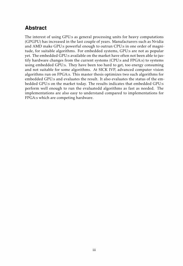
SammanfattningAbstract

The interest of using GPU:s as general processing units for heavy computations (GPGPU)has increased in the last couple of years. Manufacturers such as Nvidia and AMD makeGPU:s powerful enough to outrun CPU:s in one order of magnitude, for suitable algorithms.For embedded systems, GPU:s are not as popular yet. The embedded GPU:s available on themarket have often not been able to justify hardware changes from the current systems (CPU:sand FPGA:s) to systems using embedded GPU:s. They have been too hard to get, too energyconsuming and not suitable for some algorithms. At SICK IVP, advanced computer visionalgorithms run on FPGA:s. This master thesis optimizes two such algorithms for embeddedGPU:s and evaluates the result. It also evaluates the status of the embedded GPU:s on themarket today. The results indicates that embedded GPU:s perform well enough to run theevaluatedd algorithms as fast as needed. The implementations are also easy to understandcompared to implementations for FPGA:s which are competing hardware.

NyckelordKeywords Embdedded GPU, Computer Vision, CUDA

http://urn.kb.se/resolve?urn=urn:nbn:se:liu:diva-XXXXX

Abstract

The interest of using GPU:s as general processing units for heavy computations(GPGPU) has increased in the last couple of years. Manufacturers such as Nvidiaand AMD make GPU:s powerful enough to outrun CPU:s in one order of magni-tude, for suitable algorithms. For embedded systems, GPU:s are not as popularyet. The embedded GPU:s available on the market have often not been able to jus-tify hardware changes from the current systems (CPU:s and FPGA:s) to systemsusing embedded GPU:s. They have been too hard to get, too energy consumingand not suitable for some algorithms. At SICK IVP, advanced computer visionalgorithms run on FPGA:s. This master thesis optimizes two such algorithms forembedded GPU:s and evaluates the result. It also evaluates the status of the em-bedded GPU:s on the market today. The results indicates that embedded GPU:sperform well enough to run the evaluatedd algorithms as fast as needed. Theimplementations are also easy to understand compared to implementations forFPGA:s which are competing hardware.

iii

Acknowledgments

This project could not have been executed without the help from Johan Petters-son and Johan Hedborg. Thank you very much! I would also like to thank ErikRingaby and Klas Nordberg from CVL for their help.

Linköping, June 2014Mattias Nilsson

v

Contents

Notation xi

1 Introduction 11.1 Background . . . . . . . . . . . . . . . . . . . . . . . . . . . . . . . 11.2 Purpose and goal . . . . . . . . . . . . . . . . . . . . . . . . . . . . 21.3 Delimitations . . . . . . . . . . . . . . . . . . . . . . . . . . . . . . . 21.4 Hardware . . . . . . . . . . . . . . . . . . . . . . . . . . . . . . . . . 3

2 Sequential Algorithms 52.1 Rectification of images . . . . . . . . . . . . . . . . . . . . . . . . . 52.2 Pattern recognition . . . . . . . . . . . . . . . . . . . . . . . . . . . 6

2.2.1 Normalized cross correlation . . . . . . . . . . . . . . . . . 72.2.2 Scaling and rotation . . . . . . . . . . . . . . . . . . . . . . . 72.2.3 Complexity . . . . . . . . . . . . . . . . . . . . . . . . . . . 82.2.4 Sequential implementation . . . . . . . . . . . . . . . . . . 82.2.5 Pyramid image representation . . . . . . . . . . . . . . . . . 92.2.6 Non maxima suppression . . . . . . . . . . . . . . . . . . . 10

3 Parallel programming in theory and practise 133.1 GPU-programming . . . . . . . . . . . . . . . . . . . . . . . . . . . 13

3.1.1 Memory latency . . . . . . . . . . . . . . . . . . . . . . . . . 133.1.2 Implementation . . . . . . . . . . . . . . . . . . . . . . . . . 16

3.2 Parallel programming metrics . . . . . . . . . . . . . . . . . . . . . 183.2.1 Parallel time . . . . . . . . . . . . . . . . . . . . . . . . . . . 183.2.2 Parallel speed-up . . . . . . . . . . . . . . . . . . . . . . . . 183.2.3 Parallel Efficiency . . . . . . . . . . . . . . . . . . . . . . . . 193.2.4 Parallel Cost . . . . . . . . . . . . . . . . . . . . . . . . . . . 193.2.5 Parallel work . . . . . . . . . . . . . . . . . . . . . . . . . . . 193.2.6 Memory transfer vs. Kernel execution . . . . . . . . . . . . 193.2.7 Performance compared to bandwidth . . . . . . . . . . . . . 19

3.3 Related Work . . . . . . . . . . . . . . . . . . . . . . . . . . . . . . . 20

4 Method 21

vii

viii Contents

4.1 Initial phase . . . . . . . . . . . . . . . . . . . . . . . . . . . . . . . 214.2 Parallelization . . . . . . . . . . . . . . . . . . . . . . . . . . . . . . 224.3 Theoretical evaluation . . . . . . . . . . . . . . . . . . . . . . . . . 224.4 Implementation . . . . . . . . . . . . . . . . . . . . . . . . . . . . . 224.5 Evaluation . . . . . . . . . . . . . . . . . . . . . . . . . . . . . . . . 224.6 Alternative methods . . . . . . . . . . . . . . . . . . . . . . . . . . . 23

4.6.1 Theoretical method . . . . . . . . . . . . . . . . . . . . . . . 234.6.2 One algorithm . . . . . . . . . . . . . . . . . . . . . . . . . . 234.6.3 Conclusions . . . . . . . . . . . . . . . . . . . . . . . . . . . 23

5 Rectification of images 255.1 Generating test data . . . . . . . . . . . . . . . . . . . . . . . . . . . 255.2 Theoretical parallelization . . . . . . . . . . . . . . . . . . . . . . . 285.3 Theoretical evaluation . . . . . . . . . . . . . . . . . . . . . . . . . 295.4 Implementation . . . . . . . . . . . . . . . . . . . . . . . . . . . . . 29

5.4.1 Initial implementation . . . . . . . . . . . . . . . . . . . . . 295.4.2 General problems . . . . . . . . . . . . . . . . . . . . . . . . 305.4.3 Texture memory . . . . . . . . . . . . . . . . . . . . . . . . . 315.4.4 Constant memory . . . . . . . . . . . . . . . . . . . . . . . . 31

5.5 Results . . . . . . . . . . . . . . . . . . . . . . . . . . . . . . . . . . 315.5.1 Memory transfer . . . . . . . . . . . . . . . . . . . . . . . . 325.5.2 Kernel execution . . . . . . . . . . . . . . . . . . . . . . . . 325.5.3 Memory access performance . . . . . . . . . . . . . . . . . . 33

5.6 Discussion . . . . . . . . . . . . . . . . . . . . . . . . . . . . . . . . 345.6.1 Performance . . . . . . . . . . . . . . . . . . . . . . . . . . . 345.6.2 Memory transfer . . . . . . . . . . . . . . . . . . . . . . . . 355.6.3 Complexity of the software . . . . . . . . . . . . . . . . . . 355.6.4 Compatibility and Scalability . . . . . . . . . . . . . . . . . 35

5.7 Conclusions . . . . . . . . . . . . . . . . . . . . . . . . . . . . . . . 35

6 Pattern Recognition 376.1 Sequential Implementation . . . . . . . . . . . . . . . . . . . . . . . 376.2 Generating test data . . . . . . . . . . . . . . . . . . . . . . . . . . . 376.3 Assuring the correctness of results . . . . . . . . . . . . . . . . . . 386.4 Theoretical parallelization . . . . . . . . . . . . . . . . . . . . . . . 39

6.4.1 Pyramid image representation . . . . . . . . . . . . . . . . . 406.4.2 Parallelizing using reduction . . . . . . . . . . . . . . . . . 40

6.5 Theoretical evaluation . . . . . . . . . . . . . . . . . . . . . . . . . 416.5.1 Searching intuitive in full scale . . . . . . . . . . . . . . . . 416.5.2 Trace searching intuitive . . . . . . . . . . . . . . . . . . . . 416.5.3 Search using reduction . . . . . . . . . . . . . . . . . . . . . 426.5.4 Memory transfer vs. kernel execution . . . . . . . . . . . . 426.5.5 PMPS . . . . . . . . . . . . . . . . . . . . . . . . . . . . . . . 43

6.6 Implementation . . . . . . . . . . . . . . . . . . . . . . . . . . . . . 436.6.1 Implementation of reduction in general . . . . . . . . . . . 446.6.2 Reduction for pattern recognition . . . . . . . . . . . . . . . 44

Contents ix

6.6.3 Implementation of non maxima suppression . . . . . . . . 466.7 Results . . . . . . . . . . . . . . . . . . . . . . . . . . . . . . . . . . 46

6.7.1 Kernel performance . . . . . . . . . . . . . . . . . . . . . . . 466.7.2 Performance of algorithm . . . . . . . . . . . . . . . . . . . 466.7.3 PMPS . . . . . . . . . . . . . . . . . . . . . . . . . . . . . . . 476.7.4 Memory access performance and bandwidth . . . . . . . . 48

6.8 Discussion . . . . . . . . . . . . . . . . . . . . . . . . . . . . . . . . 496.8.1 Intuitive implementation . . . . . . . . . . . . . . . . . . . . 496.8.2 Reduction implementation . . . . . . . . . . . . . . . . . . . 506.8.3 CPU . . . . . . . . . . . . . . . . . . . . . . . . . . . . . . . . 51

6.9 Conclusions . . . . . . . . . . . . . . . . . . . . . . . . . . . . . . . 51

7 Conclusions 537.1 Overall Conclusions . . . . . . . . . . . . . . . . . . . . . . . . . . . 53

7.1.1 Recommendation about hardware . . . . . . . . . . . . . . 547.2 Future . . . . . . . . . . . . . . . . . . . . . . . . . . . . . . . . . . . 55

7.2.1 Architecture . . . . . . . . . . . . . . . . . . . . . . . . . . . 557.2.2 Implementation . . . . . . . . . . . . . . . . . . . . . . . . . 55

7.3 Evaluation of method . . . . . . . . . . . . . . . . . . . . . . . . . . 567.4 Work in a broader context . . . . . . . . . . . . . . . . . . . . . . . 56

Bibliography 57

Notation

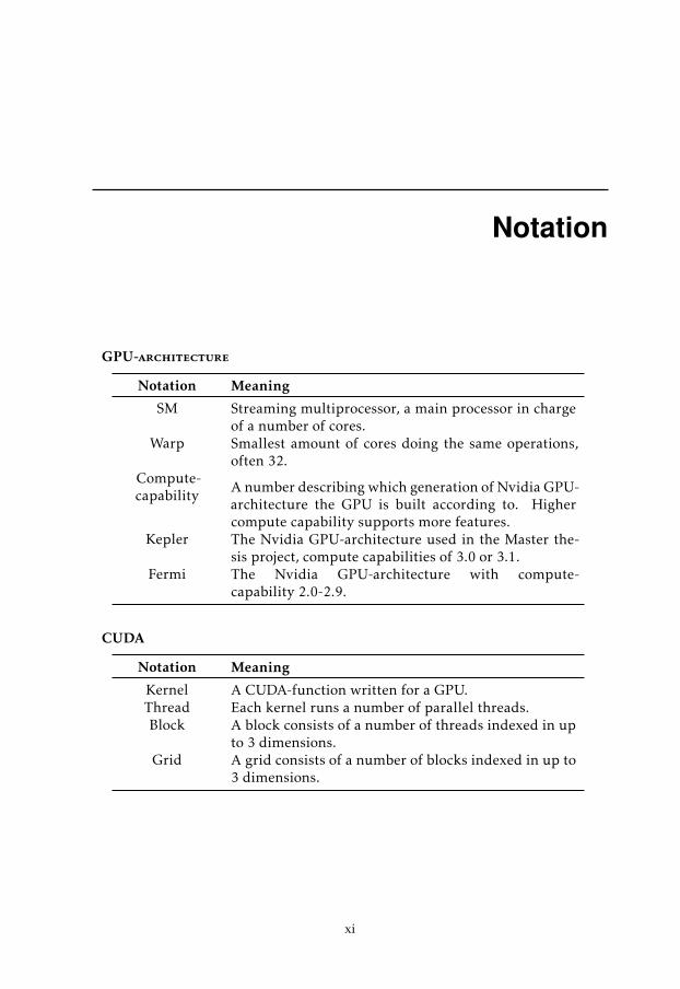
GPU-architecture

Notation Meaning

SM Streaming multiprocessor, a main processor in chargeof a number of cores.

Warp Smallest amount of cores doing the same operations,often 32.

Compute-capability A number describing which generation of Nvidia GPU-

architecture the GPU is built according to. Highercompute capability supports more features.

Kepler The Nvidia GPU-architecture used in the Master the-sis project, compute capabilities of 3.0 or 3.1.

Fermi The Nvidia GPU-architecture with compute-capability 2.0-2.9.

CUDA

Notation Meaning

Kernel A CUDA-function written for a GPU.Thread Each kernel runs a number of parallel threads.Block A block consists of a number of threads indexed in up

to 3 dimensions.Grid A grid consists of a number of blocks indexed in up to

3 dimensions.

xi

1Introduction

1.1 Background

The interest of using GPU:s as general processing units for heavy computations(GPGPU) has increased in the last couple of years. Manufacturers as Nvidia andAMD make GPU:s powerful enough to outrun CPU:s in one order of magnitude,for suitable algorithms.

Embedded GPU:s are small GPU:s built into SoC:s (System on Chips). SoC:s areintegrated circuits where several processor and function blocks are built into onechip. SoC:s are used in embedded systems such as mobile phones. The interest ofusing embedded GPU:s as general processing units have not been nearly as highas for regular GPU:s yet. The embedded GPU:s available on the market have oftennot been able to justify hardware changes from the current systems (CPU:s andFPGA:s) to systems using embedded GPU:s. They have been hard to get since themodels available on the market have been few. Their energy consumption havebeen to high and thet have not been suitable for some algorithms. However, theperformance of embedded GPU:s improve all the time and it is very likely thattheir performance will be sufficient in the foreseeable future.

At SICK IVP advanced computer vision algorithms are accelerated on FPGA:s.Accelerating the algorithms on embedded GPU:s instead might be preferred forseveral reasons. Apart from possibly being faster, GPU:s are also in general easierto program than FPGA:s. This is because the programming model of a GPU ismuch more similar to a CPU than the programming model of an FPGA is.

1

2 1 Introduction

1.2 Purpose and goal

The goal of the master thesis is to analyse how some of the computer vision algo-rithms that SICK IVP today run on FPGA:s instead would suit running on GPU:s.Critical factors in the analysis are theoretical parallelization, memory access pat-tern, memory choice and how good the performance is in practise.

Another goal is to determine whether the embedded GPU:s available today aregood enough to be considered in computer vision products. The results fromthe algorithms relate to this question in several important ways by answering thefollowing questions.

• How well is the algorithm parallelized?

• What is the performance of the implemented algorithms compared to whatwas theoretically expected?

• How device specific are the implementations, i.e. how portable are they?

• Is the performance sufficient?

• Is the code hard to understand, compared to a CPU implementation andcompared to an FPGA implementation?

When the algorithms were implemented and evaluated, so that the previous ques-tions could be answered, a recommendation about hardware was done for SICKIVP based on the answers.

1.3 Delimitations

To define the project and to scale it down to a reasonable size some delimitationswere made. The delimitations regard implementation, hardware, number of al-gorithms and how the result of the project should be interpreted.

To get a perfect idea of the performance of computer vision algorithms on embed-ded GPU:s a large number of algorithms could be analysed and implemented. Inthis project only two algorithms were analysed.

In this project only Nvidia GPU:s were used so that the CUDA programminglanguage could be used. CUDA is a modern GPGPU programming language thatis easy to set up and use compared to other GPGPU programming languages. Formore information about hardware choice see section, 1.4.

In GPU-programming a concept called multiple streams exist. Multiple streamsare explained in section 3.1.1 and are of interest for the two different algorithmsimplemented. However multiple streams are only discussed theoretically andnot implemented.

The recommendation about embedded GPU:s in products, mentioned in section1.2, is only based on the questions of the same section. Other factors that couldbe interesting for a hardware choice are not considered.

1.4 Hardware 3

1.4 Hardware

Nvidia Tegra is Nvidia:s product series of SoC:s. They are embedded devices withboth CPU:s and GPU:s on the same chip. Three different hardware set-ups wereused during the project. Most of the development were performed on a desk-top computer featuring a GTX 680 GPU. At the start of the master thesis projectthere were no devices or test boards on the market that ran embedded GPU:s withunified shader architecture. In a unified shader architecture all streaming multi-processors (SM:s)can be used for GPGPU operations but in a non-unified shaderarchitecture some SM:s are reserved for specific graphic operations. Devices with-out unified shader architecture can therefore not be utilized to their full capacityby GPGPU operations. To simulate an embedded device with unified shader ar-chitecture, tests were run on a test board featuring an Nvidia Tegra 3 with a sep-arate Geforce GT 640 GPU. Nvidia calls this combination Kayla [Nvidia, 2013].The separate GPU is there to simulate future devices with unified shader architec-ture. NVIDIA Tegra K1 has a GPU based on Kepler architecture which includesunified shaders. There are some differences between the Kayla platform and theK1 though. A big performance difference between the Kayla platform and theTegra K1 is that the the Tegra only have one SM, the separate GPU of Kayla hastwo SM:s. Another difference is that the K1 has a GPU and a CPU with a sharedmemory pool. This kind of memory drastically reduces the transfer time betweenthe CPU and GPU. A third important difference is that the memory bandwidthis higher on the GPU of Kayla, making memory accesses faster. At the end ofthe project all tests were run on a test board called Jetson TK1 featuring a K1SoC. All GPU:s used in the project are based on Kepler architecture, which is thearchitecture of a specific generation of Nvidia GPU:s.

Some important specifications of the GTX 680, the GT 640 and the Tegra K1 arelisted in table 1.1. Since accessing the global memory is a typical bottleneck of aGPU-kernel the memory bandwidth is very important. Core speed is importantto be able to make computations as fast as possible. For all GPU:s built on Keplerarchitecture an SM contains 192 cores. Therefore the number of SM:s determinesthe total number of cores.

Feature GTX 680 GT 640 Tegra K1

Memory Bandwidth 192 GB/s 29 GB/s 17 GB/sCore speed 1053MHz 1033 MHz 950 MHzNumber of SMs 8 2 1

Table 1.1: Specification for the devices targeted in the master thesis.

2Sequential Algorithms

Many computer vision algorithms are suited for running on GPU:s and the algo-rithms chosen for this master thesis project were:

• Rectification of images

• Pattern recognition using normalized cross correlation

The purpose of the first algorithm is to extract a geometrical plane from an imagewith respect to the distortion of the camera lens. It was chosen for the projectsince it is of low complexity. The second algorithm tries to find an object in animage using the intensity of the pixels. It was chosen for the project since it isa common computer vision algorithm of high complexity and because it is, incontrast to the first algorithm, not intuitively well suited for a GPU.

2.1 Rectification of images

The rectification algorithm applies to when a camera is stationed to capture aplain surface. Even though an image where the camera is placed over the surfacepointing straight down on it is wanted, see figure 2.1, it is often not desirable toinstall the camera that way e.g. because the camera may cast a shadow on thesurface. The camera is often placed around 45 degrees compared to the surface,see figure 2.1. The purpose of the algorithm is to extract parts of the image us-ing a given homography and lens distortion parameters. Given the homographybetween the image plane and the surface it is possible to transform the image tobe placed in the image plane. Let X be a coordinate in the original image, H thehomography between the surface and the image plane and Y the coordinate inthe transformed image. X and Y are written in homogeneous form.

5

6 2 Sequential Algorithms

Figure 2.1: Camera placed orthogonal to the surface to the left and approxi-mately with approximately 45 degrees angle to the right.

Y ∼ HX (2.1)

This transformation is not sufficient since the camera is using a lens that has lensdistortion. The most significant lens distortions is the radial distortion [Janez Pers,2002]. Radial distortion can be corrected according to equation 2.2.

xcorrected = x(1 + k1r2 + k2r

4 + k3r6...)

ycorrected = y(1 + k1r2 + k2r

4 + k3r6...)

(2.2)

where kn is the nth radial distortion parameter, r is the radial distance from theoptical centre of the picture, x and y are the original coordinates and xcorrectand ycorrect are the corrected coordinates. If the result is not good enough it ispossible to also add tangential distortion to the model. For most applications itis sufficient to correct for radial distortion.

The work flow of the algorithm is to go through all pixels in the output imageand make the transformation and lens correction backwards to find the correctplace in the input image. Interpolation between the neighbouring pixels in theinput image is then performed to get subpixel accuracy.

2.2 Pattern recognition

Pattern recognition, also known as template matching [Lewis, 1995], is an algo-rithm that aims to find occurrences of a known pattern in an image using thepixel values. It searches by moving the pattern through the search image andcalculating a match-value pixel by pixel, see figure 2.2 The match-value can becalculated in different ways. In this project normalized cross correlation (NCC)is used.

2.2 Pattern recognition 7

Figure 2.2: Performing NCC on each pixel of the image.

2.2.1 Normalized cross correlation

Let P be a template image with width w and height h. Let Sx be the overlappingpart of search image S when placing P around a certain pixel a. S and P arethe mean-values of the search and template image around a. The normalizedcross-correlation, C, for that image is defined in equation 2.3, [Lewis, 1995].

Ca = 1 −∑w,hi=1,j=1(Sa(i, j) − Sa)(P (i, j) − P )√∑w,h

i=1,j=1(Sa(i, j) − Sa)2 ∑w,hi=1,j=1(P (i, j) − P )2

(2.3)

Since NCC takes the mean-value and standard-deviation of the image in accountit is not as sensitive to illumination differences as it would be if regular correla-tion was used.

When NCC is calculated for all coordinates in the image, the result is a new imageconsisting of NCC-values.

2.2.2 Scaling and rotation

The algorithm can be constructed to be rotation and scale invariant by using trans-formations. In the project a rotation invariant version was implemented.

In the rotation invariant version a number of angles are chosen. For each anglethat is chosen a separate image of NCC-values is calculated to find occurrencesof the pattern rotated by that angle. When the NCC is calculated for a specificpixel at a specific angle, every coordinate in the pattern is rotated using a rotationmatrix based on that angle, see equation 2.4. Each coordinate is then added tothe coordinate of the pixel for which the NCC is calculated for. The result ofthe addition is the coordinate in the search image that should be compared withthe original coordinate of the pattern. The rotation often results in floating point


indexes. An interpolation between the closest pixels in the search image aroundthe indexes is therefore required. Bilinear interpolation is often chosen for thistype of interpolation. To make the image rotate around its optical center insteadof its upper left corner the coordinates of the pattern are in range [−w/2, w/2] and[−h/2, h/2].

The rotation invariant version searches for matches by rotating the pattern in achosen number of angles. It then calculates one image of NCC-values per angle.The index in the pattern is rotated by the transformation in equation 2.4, wherexSa , ySa are coordinates in the local search image and xp, yp are coordinates in thepattern.

(xSaySa

)=

(cos(θ) sin(θ)−sin(θ) cos(θ)

)·(xPyP

)(2.4)

2.2.3 Complexity

The rotation variant and scale variant algorithm is of the complexityO(wP hPwShS )[James Maclean, 2008] where wp and hp is width and height of the pattern andwP and hP is the width and height of the search image. Making it scale invariantand rotation invariant increases the complexity to O(rswP hPwShS ) where r is thenumber of rotations and s is the number of scales. These calculations assume thatthe mean and standard-deviation of the images is already known. Calculating themean has the complexity O(wP hP ) and can be disregarded. However calculatingthe mean of all local search images is of complexity O(wP hPwShS ) and can not bedisregarded.

2.2.4 Sequential implementation

When running the algorithm on a CPU or GPU it would be better to be able tocalculate the sums in equation 2.3 and the mean of Sa in the same loop insteadof in two separate loops. The mathematical complexity does not differ but theoverhead of running a loop on a computer makes it faster to perform severaloperations in the same loop than performing one operation in several loops. Byrewriting the sum

∑ni=1(ai − a)2, where ai are pixel values and a is the mean of

picture a, it is possible to separate the pixel values and the mean.

n∑i=1

(ai − a)2 =n∑i=1

(a2i − 2aia + a2) =

n∑i=1

a2i +

n∑i=1

a2 − 2n∑i=1

aia =

n∑i=1

a2i + na2 − 2a

n∑i=1

ai =n∑i=1

a2i + na2 − 2na2 =

n∑i=1

a2i − na

2

In the same way it is possible to rewrite the sum∑ni=1(ai − a)(bi − b), where b is

another picture of the same size, to separate the pixel values and the mean.


n∑i=1

(ai − a)(bi − b) =n∑i=1

(aibi − abi − aib + ab) =

n∑i=1

(aibi) −n∑i=1

abi −n∑i=1

aib +n∑i=1

abi =n∑i=1

(aibi) − nab − nab + nab =

n∑i=1

(aibi) − nab

By using the rewritten sums, the mean of the overlapping image Sa can be calcu-lated simultaneously as the other sums, thereby reducing the number of loops to1 instead of 2. The average of the pattern and the square sum of the pattern iscalculated offline since they will be the same for every NCC-pixel. Three sumsare calculated online for each NCC-pixel.The sums that are calculated are:

•∑Si - to be able to calculate S

•∑S2i - for the denominator in NCC

•∑SiPi- To be able to calculate

∑(Si − S)(Pi − P )

When the sums are calculated they are converted to the sums in equation 2.3.The NCC-value is calculated and the value of the pixel in the result image is set.These operations are repeated for all pixels so that the result image is filled withNCC-values.

2.2.5 Pyramid image representation

In this project full scale pattern recognition is defined as calculating the NCC forall pixels in the search image. Because of the high complexity of the full scalepattern recognition algorithm an image pyramid representation is often used toreduce the complexity, see [James Maclean, 2008]. The original images are down-sampled to create an image pyramid of a desired number of levels. The full scalepattern recognition is only performed on the coarsest level. When matches arefound on the coarsest level the matching coordinates are changed to match animage with a finer scale. In the larger image the NCC is only calculated for theresulting pixel from the previous image and its neighbouring pixels. If any ofthe neighbouring pixels have a better correlation the index will be changed tothe better match. The search in the finer images is in this report called tracesearch. The total number of operations performed when using an image pyramidis significantly lower then when performing a full scale pattern search on theoriginal image. The number of operations O is illustrated in equation 2.5.

O =rswP hPwShS

16k+

k∑i=1

mwphp

16k−i(2.5)


In equation 2.5 k is the number of times the pattern and search image are down-sampled and m is the number of matches that are saved from the original searchimage. The coefficient in the denominator is 16 because when the width andheight of the search image and pattern is down scaled by 2, the total scale factorwill be 24 = 16. The single term in equation 2.5 is the number of operations in thefull scale search on the coarsest image. The sum is the total number of operationsfor scaling up coordinates to fit finer images and calculating the matches of theneighbourhoods. To use initial matches to go from coarser images to finer imagesis hereby called trace search.

2.2.6 Non maxima suppression

Non maxima suppression is used to suppress all image-values where a neighbour-ing value is higher than the current value. Applying non maxima suppression tothe NCC-images will make regions of high correlation values result in only onehigh value. Since very few pixels are examined at finer levels it is very importantthat only one pixel per correct match is saved. Non maximum suppression, seealgorithm 1 is performed on all NCC-images on the coarsest level to get uniqueresults to use in the trace search. A rough description of the complete algorithmcan be seen in algorithm 2.

Data: imagefor all pixels (x,y) in image do

if max(neighbouring pixels) > pixel thenpixel = 0;

endendAlgorithm 1: Non maximum suppression of image. If any of the neighbouringpixels have a higher value than the current one its value is set to zero.

When using a large number of different angles in the search there is a risk thatseveral angles of the same pixel will produce high NCC-values. A better nonmaxima suppression would suppress not only in the x and y-dimension, but alsofor the closest different angles. This kind of suppression was not implementedin the project, mainly because in practise the angles searched for are often so fewthat only the best angle will produce a NCC-value high enough to be considereda match. A larger area to examine when suppressing could also be used, butsuppressing only according to the neighbouring pixels was found sufficient for


the project.

Data: patternPyramid, searchImagePyramid, minSimilarityResult: bestMatchesfor all angles do

image = performNCC(coarsestImages, angle);image = nonMaximumSupress(image);bestMatches = findBestMatches(image, bestMatches);

endfor all larger images do

upScaleIndexes(bestMatches);traceSearch(currentImageSize, bestMatches);removeBadMatches(bestMatches, similarity);

endAlgorithm 2: Pseudo code for finding a pattern in an image. The images in theimage pyramids differ by a factor 2 of size in width and height.

W.James MacLean and John K. Tsotsos proposed a similar algorithm.[James Maclean,2008].

3Parallel programming in theory and

practise

3.1 GPU-programming

When programming a GPU there are a number of features that need to be con-sidered. GPU:s use SIMD architecture (Single instruction multiple data). SIMDmeans that there are several cores running, often many and they all perform thesame operations. The only difference between them is that they take differentdata as input. The bottleneck of the performance when programming GPU:s areoften the bandwidth of different memories, see section 3.1.1.

Applications written in the CUDA programming language manages the SIMD-architecture in an efficient way. A grid of 1, 2 or 3 dimensions is used to index therunning threads of a function. The grid is divided into blocks that are calculatedspread on several streaming multiprocessors (SM:s). An important note is that inthe CUDA programming language are functions called kernels and they shall notto be mistaken for cores or processors.

3.1.1 Memory latency

A typical problem when programming a GPU is that the transfer between differ-ent memories is a bottleneck. There are different kind of memory transfers andthey are often slow if they are not chosen and implemented with care. The mostimportant memories in GPU:s are:

• Global memory

• Constant memory

• Texture memory

13

14 3 Parallel programming in theory and practise

• Shared memory

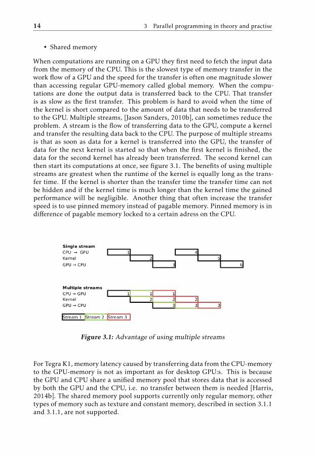
When computations are running on a GPU they first need to fetch the input datafrom the memory of the CPU. This is the slowest type of memory transfer in thework flow of a GPU and the speed for the transfer is often one magnitude slowerthan accessing regular GPU-memory called global memory. When the compu-tations are done the output data is transferred back to the CPU. That transferis as slow as the first transfer. This problem is hard to avoid when the time ofthe kernel is short compared to the amount of data that needs to be transferredto the GPU. Multiple streams, [Jason Sanders, 2010b], can sometimes reduce theproblem. A stream is the flow of transferring data to the GPU, compute a kerneland transfer the resulting data back to the CPU. The purpose of multiple streamsis that as soon as data for a kernel is transferred into the GPU, the transfer ofdata for the next kernel is started so that when the first kernel is finished, thedata for the second kernel has already been transferred. The second kernel canthen start its computations at once, see figure 3.1. The benefits of using multiplestreams are greatest when the runtime of the kernel is equally long as the trans-fer time. If the kernel is shorter than the transfer time the transfer time can notbe hidden and if the kernel time is much longer than the kernel time the gainedperformance will be negligible. Another thing that often increase the transferspeed is to use pinned memory instead of pagable memory. Pinned memory is indifference of pagable memory locked to a certain adress on the CPU.

Figure 3.1: Advantage of using multiple streams

For Tegra K1, memory latency caused by transferring data from the CPU-memoryto the GPU-memory is not as important as for desktop GPU:s. This is becausethe GPU and CPU share a unified memory pool that stores data that is accessedby both the GPU and the CPU, i.e. no transfer between them is needed [Harris,2014b]. The shared memory pool supports currently only regular memory, othertypes of memory such as texture and constant memory, described in section 3.1.1and 3.1.1, are not supported.

3.1 GPU-programming 15

Coalescing memory accesses

In regular memory the data is stored in horizontal lines. Since all threads that runon an SM are performing the same tasks, they will access the global memory atapproximately the same time. If neighbouring threads access neighbouring datain the memory several threads can get their desired data on the same read fromthe global memory. In this way, the number of accesses to the global memory canbe reduced dramatically, see figure 3.2.

Figure 3.2: Perfect coalescing in the upper image and a bad memory accesspattern below.

Shared vs. global memory

In addition to the global regular memory each SM have a local memory calledshared memory which is shared for all threads in a block. A typical GPU datatransfer bottleneck is accessing global memory of the GPU from a thread. Theshared memory is smaller than the regular memory and accessing it is faster. If akernel uses many accesses to the global memory, the values can be stored in theshared memory to reduce accesses to the global memory [Jason Sanders, 2010c].If a value is read from memory several times it is always beneficial to read it oncefrom the global memory and the rest of the times from the shared memory. Whenthe value has been read from the global memory it should be stored in the sharedmemory so it can be reached from there for the future readings.

On newer GPU:s, based on Fermi or Kepler architecture, it is not as crucial to useshared memory as for earlier architectures. This is since Fermi introduced built


in caches for each SM. The cache is using the shared memory to store the values.Consideration of shared memory is still important for maximum performance[Ragnemalm, 2013].

Constant memory

If a value is read from many different threads in a kernel it is preferred to storeit in the constant memory for increasing the performance. The constant memoryhas a fast cache accessible from the whole GPU [Jason Sanders, 2010a]. Globalmemory is only cached on every SM or block since it uses the shared memory.Values that are read from all blocks will therefore require less memory bandwidthwhen placed in the constant memory. It is constant because it can only be readfrom the GPU, it is set during a memory transfer from the CPU.

Texture memory

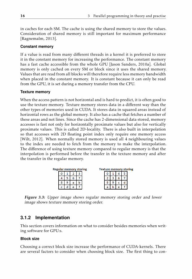
When the access pattern is not horizontal and is hard to predict, it is often good touse the texture memory. Texture memory stores data in a different way than theother types of memories used in CUDA. It stores data in squared areas instead ofhorizontal rows as the global memory. It also has a cache that fetches a number ofthese areas and not lines. Since the cache has 2-dimensional data stored, memoryaccesses is fast not only for horizontally proximate values but also for verticallyproximate values. This is called 2D-locality. There is also built in interpolationso that accesses with 2D floating point index only require one memory access[Wilt, 2012]. When normally stored memory is used all 4 neighbouring valuesto the index are needed to fetch from the memory to make the interpolation.The difference of using texture memory compared to regular memory is that theinterpolation is performed before the transfer in the texture memory and afterthe transfer in the regular memory.

Figure 3.3: Upper image shows regular memory storing order and lowerimage shows texture memory storing order.

3.1.2 Implementation

This section covers information on what to consider besides memories when writ-ing software for GPU:s.

Block size

Choosing a correct block size increase the performance of CUDA-kernels. Thereare several factors to consider when choosing block size. The first thing to con-

3.1 GPU-programming 17

sider is how many SM:s the GPU running the kernel has. The workload should bedivided in at least as many blocks as there are SM:s so that all SM:s will be busy.

Another important thing when choosing block size is that the block size is a multi-ple of the warp size. The warp size is the smallest amount of threads performingthe same operation. The GPU is always running a multiple of warps doing thesame thing [Jason Sanders, 2010a]. If a block does have fewer threads it will berounded up to the next multiple of the block size and those resources will bewasted. So if the warp size is 32 and 33 three threads are chosen for a kernel64 threads will be used and 31 of them will idle. The wasted resources can becalculated according to:

rwasted =w − b%wwdb/we

(3.1)

where rwasted are the wasted resources [0, 1], w is the warp size, b is the block sizeand % calculates the remainder of a division. Note that no resources are wastedif the block size is a multiple of the warp size. The equation is invalid if the blocksize is a multiple of the warp size.

Partition work between CPU and GPU

As mentioned in section 1.1, GPU:s outrun CPU:s by one order of a magnitudefor many algorithms. There are also many algorithms where parts or the wholealgorithm run faster on a CPU than on a GPU, especially parts that are not paral-lelizable at all. Therefore it is important to evaluate which part of an algorithmthat might run faster on a CPU. Since the Tegra K1 has a shared memory poolbetween the CPU and the GPU, the overhead of switching from CPU to GPU isreduced, resulting in more situations where it is favourable to switch betweenCPU and GPU.

Shuffling

A new feature of the Kepler architecture is that it is possible to share data betweendifferent threads in a warp without using shared memory. When a variable is readusing shuffle all threads will read the value of the variable in the neighbouringthread, instead of the local thread, one or several steps away. Shuffle one stepwill read the variable of thread 0 in thread 1 etc. This way of reading data iseven faster than using shared memory since only one read operation is required.Shared memory needs write, synchronize and read. Another benefit of usingshuffling compared to using shared memory is that the size of the shared memoryis small. The joint size of all the registers from the threads is bigger than theshared memory [Goss, 2013].

Grid stride loops

In GPU-computing the number of threads is often adapted to the number of ele-ments in the array processed. This is not convenient for all algorithms e.g. if allelements in an array of 33 elements are multiplied by 2 the number of threads


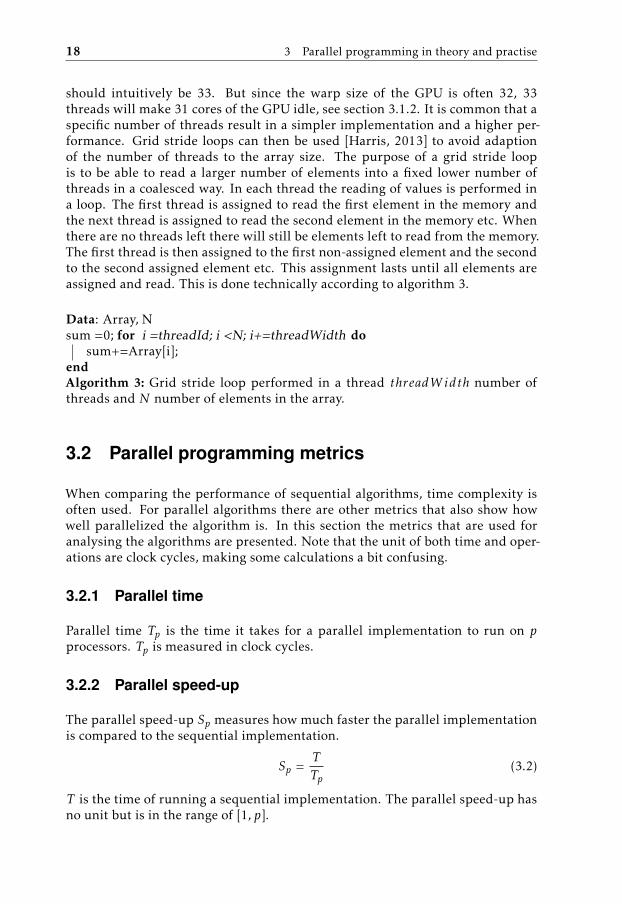
should intuitively be 33. But since the warp size of the GPU is often 32, 33threads will make 31 cores of the GPU idle, see section 3.1.2. It is common that aspecific number of threads result in a simpler implementation and a higher per-formance. Grid stride loops can then be used [Harris, 2013] to avoid adaptionof the number of threads to the array size. The purpose of a grid stride loopis to be able to read a larger number of elements into a fixed lower number ofthreads in a coalesced way. In each thread the reading of values is performed ina loop. The first thread is assigned to read the first element in the memory andthe next thread is assigned to read the second element in the memory etc. Whenthere are no threads left there will still be elements left to read from the memory.The first thread is then assigned to the first non-assigned element and the secondto the second assigned element etc. This assignment lasts until all elements areassigned and read. This is done technically according to algorithm 3.

Data: Array, Nsum =0; for i =threadId; i <N; i+=threadWidth do

sum+=Array[i];endAlgorithm 3: Grid stride loop performed in a thread threadW idth number ofthreads and N number of elements in the array.

3.2 Parallel programming metrics

When comparing the performance of sequential algorithms, time complexity isoften used. For parallel algorithms there are other metrics that also show howwell parallelized the algorithm is. In this section the metrics that are used foranalysing the algorithms are presented. Note that the unit of both time and oper-ations are clock cycles, making some calculations a bit confusing.

3.2.1 Parallel time

Parallel time Tp is the time it takes for a parallel implementation to run on pprocessors. Tp is measured in clock cycles.

3.2.2 Parallel speed-up

The parallel speed-up Sp measures how much faster the parallel implementationis compared to the sequential implementation.

Sp =TTp

(3.2)

T is the time of running a sequential implementation. The parallel speed-up hasno unit but is in the range of [1, p].

3.2 Parallel programming metrics 19

3.2.3 Parallel Efficiency

Parallel efficiency Ep measures how well an implementation scales independentof the value of p.

Ep =Spp

(3.3)

where the optimal scaling of an algorithm is 1. Ep is Sp normalized over thenumber of processors.

3.2.4 Parallel Cost

Parallel cost measures if resources are wasted when running a parallel algorithm.

Cp = pTp (3.4)

Consider the total number of clock cycles passed on a system using p processors,during a parallel time Tp, pTp. If the passed clock cycles are more than the to-tal number of clock cycles passed when running the algorithm sequentially onone processor, the parallel implementation is wasting resources. An algorithm istherefore Cost optimal if Cp = T .

3.2.5 Parallel work

The work W is the total number of operations that are performed on all proces-sors. If more operations are performed than operations performed on one proces-sor in the sequential algorithm, the parallel algorithm is doing more work thanthe sequential algorithm. An algorithm is Work optimal if the number of opera-tions performed for the parallel algorithm is equal to the operations performedby the sequential algorithm, W = T .

3.2.6 Memory transfer vs. Kernel execution

A crucial part of running computations on a GPU is transferring data between theCPU and the GPU. Sending the input data to the GPU before the computationsand the result back to the CPU after the computations is time consuming. Ananalysis of an algorithm must consider the transfer time of data. Multiplyingthe size of the data with the transfer speed on the device results in the transfertime. An interesting metric is the kernel execution time compared to the memorytransfer time.

3.2.7 Performance compared to bandwidth

The performance of a kernel can be evaluated by comparing its average memorybandwidth to the memory bandwidth of the GPU. The memory bandwidth canbe estimated by running a kernel that only copies the value from one array toanother. The quotient between the average memory access speed and the memorybandwidth is in this report called memory access performance. By dividing the sizeof the copied array by the running time of the kernel the average memory access


speed for the kernel can be calculated.

vm =whsntk

(3.5)

vm is the memory access speed, s is the size of one pixel in the image, n is thenumber of times the value is read or written to the memory and tk is the measuredtime of the kernel. A kernel with an optimal access pattern has a speed very closeto the copy kernel.

3.3 Related Work

Egil Fykse wrote a thesis [Fykse, 2013] comparing the performance of computervision algorithms running on GPU:s in embedded systems and on FPGA:s. Hisbenchmark algorithms were similar to the used algorithms in this thesis, althoughhis focus laid on implementing FPGA versions of the algorithms. The hardwareused for his GPU-implementations is not an embedded GPU, but the predecessorto the Kayla platform, CARMA. Egils conclusion is that his results are slightlyfaster for the GPU but that the FPGA is more energy efficient. The Tegra K1should be much more power efficient than CARMA since CARMA features a desk-top GPU, but this project does not examine the power usage of any devices.

4Method

The project was performed according to a method that analysed the algorithmsin steps which are described in this chapter. The parallelization, the theoreticalevaluation and the implementation were executed iteratively to be able to testnew ideas. The steps were:

• Initial phase

• Parallelization

• Theoretical evaluation

• Implementation

• Evaluation

4.1 Initial phase

In the initial phase the sequential version of the algorithm was analysed theoret-ically, by calculating its complexity, and implemented. Artificial test data wasgenerated using Matlab. The test data was in general as simple as possible. Thepurpose of the project was not to test the accuracy of the algorithms but to opti-mize the already known algorithms. Imprecise test data could result in problemswhere it would be hard to know whether undesired results was because of theaccuracy of the algorithm or because of bugs in the implementation.

21

22 4 Method

4.2 Parallelization

The parallelization was about making parallel versions of the algorithm and deter-mining which of the versions that should be implemented and further analysed.The list below describe on what premises the implementations were optimized.

• Different algorithm variants

• Memory choice

• Memory access pattern

• Partitioning between CPU and GPU

• Shuffling

• Grid stride loops

For a description of what the items in the list mean see section 3.1

4.3 Theoretical evaluation

A theoretical evaluation is a good way of determining how parallelizable an algo-rithm is. The parallel performance metrics presented in section 3.2 are used forthe theoretical evaluation. Since not all algorithms perform well on GPU:s theresult of the theoretical evaluation may differ from the result of later steps of themethod.

4.4 Implementation

The implementation was about implementing the different versions of the algo-rithm proposed in the parallelization phase as efficient as possible. Measuring ofperformance was an important part of the implementation phase. Profiling toolsmake it possible to show the performance of the different parts of the runningkernels. For this project Nvidia Visual profiler was used.

4.5 Evaluation

In the evaluation the results from the theoretical evaluation and implementationwas compared to make a conclusion supported in several ways. There were im-portant questions that needed to be answered to be able to make a conclusionabout embedded GPU:s after the 2 algorithms were analysed.

• Was the performance as expected?

• Is the performance sufficient?

• How advanced is the code compare to code for a CPU or FPGA?

4.6 Alternative methods 23

• How portable is the code?

• Is further optimization possible?

• What are the bottlenecks?

When all the algorithms were analysed, the possible conclusions about perfor-mance of embedded GPU:s in general and about the algorithms were made.

4.6 Alternative methods

The above described method is a combination of practical and theoretical work.Algorithms are both analysed theoretically, implemented and evaluated using theresults. Other approaches could be either more theoretical or laying more focuson one single algorithm.

4.6.1 Theoretical method

A theoretical method would analyse algorithms only theoretically. By using thismethod the analysis of an algorithm would take less time so that the projectwould cover more algorithms. The benefit of more algorithms is that it wouldgive a larger picture of how well computer vision algorithms are suited for em-bedded GPU:s. However implementations often reveal problems that are easilymissed when doing a theoretical evaluation. An implementation is a certificationthat something actually works and an evaluation of how well it works.

4.6.2 One algorithm

Another type of method could spend more time implementing and optimizingone single algorithm. Even better results could be achieved for the chosen algo-rithm when spending more time on it. However a lot of the optimizations regard-ing one algorithm is specific for that algorithm and does not say much about theperformance of embedded GPU:s in general. This method would not give a goodpicture of computer vision on embedded GPU:s in general.

4.6.3 Conclusions

Given the projected outcomes of the alternative methods described above theoriginally proposed method was used.

5Rectification of images

5.1 Generating test data

Synthetic test data was generated in Matlab. The first step was to create two im-ages where one had a rectangle located in the image plane, see figure 5.1. Theother picture was a geometrical object simulating a rectangle from another view,see figure 5.2. By using the edges from the rectangles and equation 2.1 a homog-raphy between the rectangles could be calculated. The homography parameterswere stored to use as input to the program running the algorithm.

Figure 5.1: Rectangle in image plane.

25

26 5 Rectification of images

Figure 5.2: Rectangle from another view.

Lens distortion was also simulated. An image distorted by specific lens distortionparameters can not be calculated analytically since equation 2.2 has no closedform solution for obtaining x from xc. An iterative numerical solution accordingto Newtons method, equation 5.1, was implemented in Matlab to simulate im-age distortion. The pseudo code for generation of lens distortion is displayed inalgorithm 4. Only radial distortion was simulated.

xn+1 = xn −f ′(xn)f (xn)

(5.1)

Data: image, maxdiff, paramResult: Distorted imagefor all pixels (x,y) in image do

Convert x and y to normalized coordinates;xi , yi = x, y;while | correct(xi , param) − x | + | correct(xi , param) − y |> maxdif f do

xi = xi + correct(xi ,param)−xi(correct(xi ,param)−xi )′

;

yi = yi + correct(yi ,param)−yi(correct(yi ,param)−yi )′

;

endConvert xi and yi to pixel range.;outimage(x, y) = interpolation(image(xi , yi));

endAlgorithm 4: Pseudo code for distorting an image. correct is the lens correctionformula. The interpolation is bilinear, maxdif f is the maximum tolerated errorand param are the distortion parameters.

The test input image was achieved by changing the perspective of the first picture

5.1 Generating test data 27

with a rectangle in the image plane and the applying lens distortion to that image,see figure 5.3. To get a reference result for the GPU rectifications, the sequentialrectification algorithm was applied to the test input image, see figure 5.4. Notethat some parts of the original image is missing. This is not an error but due tothe fact that some parts of the original image does not fit into the input image infigure 5.3.

The parameters of the homography and the lens distortion parameters are affect-ing the performance of the algorithm. If the homography makes the algorithmfetch values from a smaller rectangle there will be fewer cache misses resultingin a higher performance. The reason that there will be fewer cache misses is thata smaller rectangle has fewer pixels and a bigger percentage of the pixels can bestored in the cache. However when the algorithm is used in reality the rectanglewill always be as large as possible and still fitting the sensor. Therefore the inputdata is also constructed this way. If the lens distortion parameters are smaller theaccess pattern will be more linear which also will result in fewer cache misses.Reasonable sizes are therefore chosen for the lens distortion parameters. Thelens distortion assumes an image with normalized coordinates between [−1, 1]. Itis therefore important to transform the pixel values into normalized coordinatesto get a correct result in terms of lens correction. The lens distortion parameters,described in equation 2.2, used in this project are illustrated in equation 5.2, notethat k3 was not used.

k1 = 0.04, k2 = 0.008 (5.2)

Figure 5.3: Input image for tests.


Figure 5.4: Reference result for tests.

5.2 Theoretical parallelization

The rectification algorithm is very suitable for parallelization since lens correc-tion and homography transformation can be performed independently for eachpixel. The pseudo code for the parallelized algorithm for n pixels on n processorsis illustrated in algorithm 5.

Data: image, HResult: rectified imagefor all pixels (x,y) in parallel do

r =√x2 + y2;

xc = x(1 + k1r2 + k2r

4);yc = y(1 + k1r

2 + k2r4);

(xh, yh, 1)T ∼ H · (xc, yc, 1)T ;outImage(x, y) = interpolation(image(xh, yh));

endAlgorithm 5: Pseudo code for parallel rectification. Assumes normalized coordi-nates.

The interpolation used in the master thesis project is bilinear and it is done since(xh, yh) is typically not integers.

5.3 Theoretical evaluation 29


In this section the algorithm is theoretically evaluated according to section 3.2.As section 5.2 states, the algorithm is very suitable for parallelization. The paral-lel time Tp for p processors and n pixels is of order n/p. The parallel speed-up Spincreases proportionally when p is increasing. This gives a parallel efficiency Epof 1. The parallel cost Cp is of the order p · np = n.

Since the sequential time is of order n, the algorithm is cost optimal. The parallelwork for p processors is also of order n. The algorithm is also work optimal, seesection 3.2.5.

The slow part of a kernel is the global memory accesses. In this kernel, therewill be maximum 5 global memory accesses per thread. 4 accesses for fetchingneighbouring pixel values to interpolate between and one access to write the re-sult to the global memory. But since the GPU uses the shared memory as cache,see section 3.1.1, there will most likely be less global memory accesses dependingon the access pattern. The memory bandwidth between the CPU and GPU canbe measured but it is in general at least 10 times slower than the global mem-ory bandwidth, the factor is 24 for the GTX680 GPU. Even if all global memoryaccesses will be cache misses, the kernel will still be a lot faster than the mem-ory transfer. Equation 5.3 aims to illustrate that the kernel will be faster definitMDtH as memory transfer latency device to host and MHtD as vice versa.

MDtH + MHtD >> 5 ·GlobMemAccess · P ixels (5.3)

For the GTX 680 GPU the memory transfer should be around 485 times slower

than the kernel. Since the kernel is so much faster than the memory transfer mul-tiple streams would not increase the performance in any substantial way. Multi-ple streams are described in section 3.1.1.

5.4 Implementation

The implementation was done in steps to be able to determine how much eachstep affected the performance.

5.4.1 Initial implementation

The first implementation of the rectification was simple and intuitive. Globalmemory was used for all memory accesses. As mentioned in section 5.2 the rectifi-cation algorithm is easy to parallelize. For an Nvidia GPU from the generation ofFermi or newer, the naive implementation is quite good since the shared memoryis used as a cache. But for an older GPU without use of cache the implementationwould be slow.


Figure 5.5: Access pattern on input image in rectification.

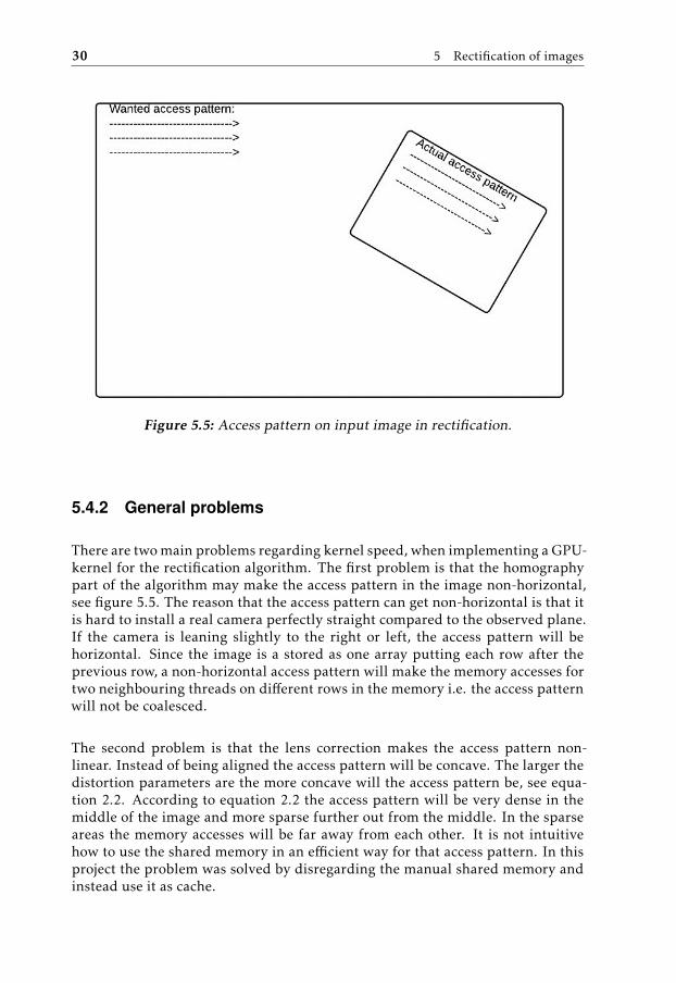
5.4.2 General problems

There are two main problems regarding kernel speed, when implementing a GPU-kernel for the rectification algorithm. The first problem is that the homographypart of the algorithm may make the access pattern in the image non-horizontal,see figure 5.5. The reason that the access pattern can get non-horizontal is that itis hard to install a real camera perfectly straight compared to the observed plane.If the camera is leaning slightly to the right or left, the access pattern will behorizontal. Since the image is a stored as one array putting each row after theprevious row, a non-horizontal access pattern will make the memory accesses fortwo neighbouring threads on different rows in the memory i.e. the access patternwill not be coalesced.

The second problem is that the lens correction makes the access pattern non-linear. Instead of being aligned the access pattern will be concave. The larger thedistortion parameters are the more concave will the access pattern be, see equa-tion 2.2. According to equation 2.2 the access pattern will be very dense in themiddle of the image and more sparse further out from the middle. In the sparseareas the memory accesses will be far away from each other. It is not intuitivehow to use the shared memory in an efficient way for that access pattern. In thisproject the problem was solved by disregarding the manual shared memory andinstead use it as cache.

5.5 Results 31

5.4.3 Texture memory

When the access pattern is irregular the performance is it often increased by us-ing texture memory instead of global memory. Interpolations are also performedvery fast using the texture memory, see section 3.1.1. The access pattern of therectification algorithm fits well into that description and the performance wereclearly increased by loading the input image to the texture memory instead of theglobal memory.

5.4.4 Constant memory

The input parameters are the same for every pixel in the image and they areread once for every thread. The performance of the implementation is drasticallyincreased when reading them from constant memory compared to reading themfrom global memory, see section 3.1.1.

5.5 Results

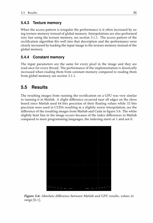
The resulting images from running the rectification on a GPU was very similarto running it in Matlab. A slight difference occurred near all edges on the chessboard since Matlab used 64 bits precision of their floating values while 32 bitsprecision were used in CUDA resulting in a slightly worse interpolation, see thedifference of the resulting images from Matlab and Cuda in figure 5.6. The whiteslightly bent line in the image occurs because of the index differences in Matlabcompared to most programming languages, the indexing starts at 1 and not 0.

Figure 5.6: Absolute difference between Matlab and GPU results, values inrange [0, 1].


The results of the different steps of the optimization are all presented below to beable to evaluate them. All results are averages over 5 runs.

5.5.1 Memory transfer

As explained in section 3.1.1 transferring data from the CPU to GPU is often abottleneck when running smaller kernels. The differences of using pagable orpinned memory, see section 3.1.1, are displayed in table 5.1. The time of thememory transfer does not affect the kernel time.

Table 5.1: Transferring image of 1024x1024 pixels 32 bit floating points be-tween CPU and GPU using pagable vs pinned memory (µs).

Task GTX 680 GT 640Pagable CPU -> GPU 703 13113Pagable GPU -> CPU 649 17810Pinned CPU -> GPU 694 12908Pinned GPU -> CPU 649 8799

On Tegra K1 no regular memory needs to be transferred between the CPU andGPU because of the unified memory pool. Data lying in the texture memoryneeds to be transferred though. The transfer of a 1024x1024 image of 32 bitfloating points to the texture memory takes about 1.1 ms.

5.5.2 Kernel execution

The results of running an rectification implementation on a 1024x1024 pixels im-age using a naive approach (only global memory), a constant memory approachand a texture memory and constant memory approach on the GTX 680 and GT640 is displayed in table 5.2.

Table 5.2: Performance of different optimization steps (µs). The implemen-tation using texture memory also uses constant memory.

Task GTX 680 GT 640Naive 392 1334Constant memory 280 960Texture memory 88 747

On Tegra K1 it is not as obvious what is the best way of optimizing the kernel.The texture memory can not be used in the unified memory pool. This means thatif the texture memory is used, more transfer between GPU and CPU is needed. Ifthe increased performance in the kernel is smaller than the lost time of memorytransfer, it is not beneficial to use the texture memory. The results of running

5.5 Results 33

the algorithm on K1 using texture memory and unified memory are illustrated intable 5.3

Table 5.3: Performance of using textured memory and global unified mem-ory on K1 (ms).

Task Tegra K1Texture memory 1.8Global unified 4.1

Since the memory transfer time of the texture memory is 1.1 ms and the reducedtime in kernel by using the texture memory is 2.3 ms it is preferred to use the tex-ture memory. Since the memory transfer time is shorter than the kernel time thelatency can theoretically also be hidden by using multiple streams. The resultingimages would then be received with a constant delay of 1.1 ms but new resultswould be received every 1.8 ms.

Table 5.2 shows that choosing texture memory instead of global memory is pre-ferred for a desktop GPU running the rectification algorithm. The data set usedfor that test is an optimal data set for the global memory. In table 5.4 the planethat is supposed to be extracted from the input image is rotated 90 degrees to theinput image making the access pattern in the input image very bad for the globalmemory, as discussed in section 5.4.2. The tests are run with 1024x1024 imagesize. The results show that for this kind of data set the texture memory is evenmore superior than for the previous data.

Table 5.4: Varying results for hard data set using textured and global mem-ory (µs).

Task GTX 680 GT 640Kernel using texture memory 89 775Kernel using global memory 659 3123

5.5.3 Memory access performance

The performance of a kernel can be evaluated by comparing its average memoryaccess speed to the memory access speed of a copy kernel, see section 3.2.7. Thememory access performance were quite good for the rectification algorithm, butit differed between the GTX 680 and the other two GPUs. The size of the inputdata was 1024x1024 and the size of each element were 4 Bytes (32-bit floatingpoints). In the kernel code there is one read and one write making n = 2. Thememory access speed on the Kayla platform is then:

1024x1024x4x2747 · 10−6 ' 11GB/s. (5.4)


The memory access speed of a copy kernel on Kayla was 27GB/s making thememory access performance 0.4.

The memory access speed of the Tegra K1 was:

1024x1024x4x21.8 · 10−3 ' 47GB/s. (5.5)

The memory bandwidth of the desktop was 11,7 GB/s making the memory accessperformance 0.4.

The memory access speed of the GTX 680 was:

1024x1024x4x288 · 10−6 ' 95GB/s. (5.6)

The memory bandwidth of the desktop was 147 GB/s making the memory accessperformance 0.64.

5.6 Discussion

As section 5.3 states, the algorithm is very suitable for parallelization. The prac-tical results also states that its performance running on an actual GPU is good.As mentioned in section 3.1.1 the bottleneck of running algorithms on GPU:s isoften the number of accesses to the global memory. When using texture memorythe rectification algorithm only performs 2 accesses per thread, except the inputparameters which are all read once for every thread.

As the results states the most important differences in performance for this al-gorithm depend on how the different memories are used. Using the constantmemory for the parameters of lens distortion and for the homography is crucialto get a good result. It is also important to use texture memory, depending onthe camera installation, see section 5.4.2 and table 5.4. The texture memory willmake the installation of the camera much easier though, since a non-horizontalaccess pattern will not decrease the performance.

5.6.1 Performance

The memory access performance of the algorithm is not very close to optimal. Thelens correction part of the algorithm makes it almost impossible to avoid cachemisses. It is possible that usage of the shared memory in a manual way couldmake the memory access performance even higher but manual shared memoryhas not been used in this project. Something that is interesting for the projectis to use the performance to calculate how much of the GPU computing time isused by the rectification. The performance goal of the rectification is that otheralgorithms should be able to run simultaneously on the GPU, keeping their per-formance. Given that 25 frames per second (fps) is needed for the other algorithmand the kernel of rectification is 1.8 ms on K1, the time used by rectification on

5.7 Conclusions 35

the GPU is approximately 1, 8ms · 25 = 0.05 or 5%. The performance goal is there-fore considered fulfilled.

5.6.2 Memory transfer

For a classic computer architecture with separate memories for the GPU and theCPU, the kernel is very fast. Although the transfer time of data from the CPU tothe GPU is slow in comparison. This memory latency can not be hidden by usingmultiple streams i.e. no matter how fast the kernel is the number of kernels thatcan be run per second is restricted by the memory transfer time. The conclusionfrom this is that for a classic computer architecture, it is better to include therectification part in another algorithm than to use it separately since the mem-ory transfer from CPU to GPU can be avoided and the memory latency will bepossible to hide by using multiple streams.

The unified memory on Tegra K1, see section 3.1.1 results in several benefits. Theobvious reason is that slow CPU-GPU memory transfers are removed and therewill be less memory latency for the kernels. Another benefit is that the host codewill be easier to read and understand because less code will be about memorytransfers.

5.6.3 Complexity of the software

The software written for the rectification algorithm is short and easy to read. Itis harder to read than software doing the same thing on a CPU though. The maindifference in readability is that management of threads using the combination ofgrids, blocks and threads is more complex than management of threads in CPU-code where one-dimensional indexes are used.

5.6.4 Compatibility and Scalability

One important task of this project was to determine the portability of the soft-ware written for a specific GPU. For the rectification algorithm there is no obvi-ous way to change the code depending on which GPU is used. Both the desktopGPU (Geforce GTX 680) and the Kayla platform (Geforce GT 640) run the samesoftware. They also perform best for approximately the same block size. The codemust be changed a bit to use unified memory on K1 though. But the code thatuse unified memory is shorter and easier to understand because of the absence ofmemory transfers.

5.7 Conclusions

The rectification algorithm works well on a GPU, especially for an embeddedGPU. The reason why it works better for an embedded GPU is because of theavoidance of memory transfer latency when using the shared memory pool. Theperformance is very high, giving the GPU a chance to perform other tasks alongwith the rectification.


The algorithm is completely parallelizable which makes it computationally lightfor a GPU. The fact that the memory access pattern is not coalesced slows downthe result though.

The software is easy to understand and is compatible for different GPU:s featur-ing the Kepler architecture. However, to get maximum performance, a correctimage size should be selected, the number of pixels should be a multiple of thewarp size, see section 3.1.2.

An obvious benefit of using embedded GPU:s compared to other hardware isthat it makes the installation easier for customers since perfect alignment of thecamera is not necessary to keep the performance up, see section 5.4.2 and figure5.4. When the direction of the camera lens gets more horizontal, the result imagefrom the rectification gets blurrier though. Similar solutions as the texture mem-ory could be implemented on other hardware but with a high developer effort.

6Pattern Recognition

6.1 Sequential Implementation

Before any parallel pattern recognition algorithm was implemented a sequen-tial implementation was made. The purpose of the sequential implementationwas to get a deeper understanding of the algorithm. Since it is very hard todebug parallel code and especially GPU-code, it is very convenient to rely ona verified CPU implementation when making a GPU-implementation. The per-formance of the sequential CPU implementation should not be compared to theGPU-implementations. Such a comparison would not be fair since no greater ef-fort has been made to optimize the performance of the sequential algorithm. Thesequential implementation was done according to algorithm 2.

6.2 Generating test data

The test data for the pattern recognition algorithm was mainly synthetic. Toassure that the images were not too noisy to get a good result, synthetic searchimages were made by pasting rotated pattern images, see image 6.1, into a largerimage, see image 6.2. However the fact that the synthetic data was noise free wasnot exploited to make a faster implementation that would fail for a noisy dataset.

37

38 6 Pattern Recognition

Figure 6.1: Example of pattern image.

Figure 6.2: Example of search image.

6.3 Assuring the correctness of results

The correctness of an implementation was assured by checking the result for asmall data set where the correct result was trivial. The search image of the trivialtest data was:

1 1 1 1 1 1 11 1 1 1 1 1 11 1 10 20 30 1 11 1 40 50 60 1 11 1 70 80 90 1 11 1 1 1 1 1 11 1 1 1 1 1 1

.

6.4 Theoretical parallelization 39

The pattern of the trivial test was:

10 20 3040 50 6070 80 90

.Since the pattern is located in the middle of the search image the result of the fullscale pattern search should propose an occurrence of the pattern at i = 4, j = 4in the search image. The NCC value of that pixel should be 1 and the angleshould be 0. To assure that rotations were handled correctly the test patternwas rotated 90 degrees. The resulting pixel should then be the same but theresulting angle should be 90 degrees. All of the GPU-implementations were notsuitable to run on as small data sets as this trivial example. In those cases anotherimplementation tested on the small data set was used. If the implementationvariant that were to be tested got the same result on a large data set as the otherimplementation did it was considered correct.

For all implementations a visual inspection was also used. Figure 6.3 displaysthe result of the visualization of the resulting matches.

Figure 6.3: Result of pattern recognition visualized.

6.4 Theoretical parallelization

There are several possible ways to parallelize the pattern recognition algorithm.The full scale NCC search that is performed first is fully parallelizable for each


pixel in the search image, see algorithm 6.

Data: searchImage, patternResult: correlationImagefor all pixels in correlationImage do

pixelResult = NCC(searchImage, pattern, pixel);correlationImage[pixel] = pixelResult;

endAlgorithm 6: Fully parallel NCC.

6.4.1 Pyramid image representation

For a large multicore system, with as many cores as pixels in the search image,this parallelization would be very fast, however the embedded GPU:s on the mar-ket do not have even close to as many cores as pixels in a search image. There-fore the pyramid image representation, described in section 2.2, is used also forthe parallel versions of the pattern search. As illustrated in algorithm 2, a tracesearch is performed at each down-sampled level of the image. This trace searchwhere the NCC value of only a few pixels is calculated is not as easy to parallelizein a good way. An intuitive solution would be to calculate the NCC for each pixelin parallel. But since only a few pixels are calculated in the trace search the totalnumber of threads will be restricted to a much smaller value than the number ofcores on the GPU. The cores that are not used for the threads will then idle andthe performance of the GPU will be low.

6.4.2 Parallelizing using reduction

A more complex way of parallelizing pattern recognition is to make a thread forevery pixel in the pattern for every NCC pixel that is calculated. In that waythe number of threads will be far larger, however there will be several threadscalculating a single NCC value. All threads calculating sums for a specific NCC-pixel must combine their sums to be able to receive an actual result. The bestapproach for combining sums in parallel is reduction. Reduction is used whenan operation is performed on a large number of elements and the operation isnot fully parallelizable but partial results can be combined to global results. Itis thereby suitable for operations such as max and sum. Reduction performsthe wanted operation on two elements at a time creating a partial result. Allavailable processors will perform this operation on different elements. When allpartial results are finished they are combined to create new partial results. Thisprocedure is repeated until there is only one element left, containing the finalvalue, see figure 6.4.

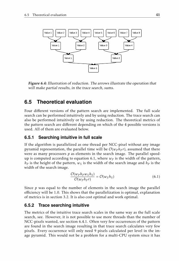
6.5 Theoretical evaluation 41

Figure 6.4: Illustration of reduction. The arrows illustrate the operation thatwill make partial results, in the trace search, sums.


Four different versions of the pattern search are implemented. The full scalesearch can be performed intuitively and by using reduction. The trace search canalso be performed intuitively or by using reduction. The theoretical metrics ofthe pattern search are different depending on which of the 4 possible versions isused. All of them are evaluated below.

6.5.1 Searching intuitive in full scale

If the algorithm is parallelized as one thread per NCC-pixel without any imagepyramid representation, the parallel time will be O(wP hP r), assumed that therewere as many processors p as elements in the search image. The parallel speed-up is computed according to equation 6.1, where wP is the width of the pattern,hP is the height of the pattern, wS is the width of the search image and hP is thewidth of the search image.

O(wP hPwShS )O(wP hP r)

= O(wShS ) (6.1)

Since p was equal to the number of elements in the search image the parallelefficiency will be 1.0. This shows that the parallelization is optimal, explanationof metrics is in section 3.2. It is also cost optimal and work optimal.

6.5.2 Trace searching intuitive

The metrics of the intuitive trace search scales in the same way as the full scalesearch, see. However, it is not possible to use more threads than the number ofNCC-pixels wanted, see section 6.4.1. Often very few occurrences of the patternare found in the search image resulting in that trace search calculates very fewpixels. Every occurrence will only need 9 pixels calculated per level in the im-age pyramid. This would not be a problem for a multi-CPU system since it has


very few processors and is made to handle few threads. However, the GPU archi-tecture has many cores and is made to process large amounts of threads at once.Running a GPU with as few as 9 threads will put most cores of the GPU in idlemode. The parallel time of the trace search is displayed in equation 6.2.

Tp =k∑i=1

hpwpr

16i(6.2)

6.5.3 Search using reduction

Parallelization using reduction scales differently than the intuitive paralleliza-tion. The process can be divided into two parts. One part for reading the datafrom global memory and one part for reducing it. The parallel time of readingthe data with p processors will be O(wP hP rp ). The parallel time of performing areduction is O(log(n)), given that p is at least half the size of the list of elementsto be reduced. With p as large as the array to be reduced, the parallel time isO(1), but the parallel time of the reduction part does not change for more proces-sors than half the number of elements to be reduced. The parallel work of thereduction part is illustrated in equation 6.3.

W =log(n)∑i=1

n

2i=log(n)−1∑i=0

n

2i+1=n2

log(n)−1∑i=1

(12

)i=n2

1 − (1/2)log(n)

1 − (1/2)= n(1−(1/2)log(n)) = n−1

(6.3)

The number of operations needed to perform the summation sequentially insteadof using reduction is also n − 1. The reducing part of reduction is thereby workoptimal. To be cost optimal, the parallel time of the reduction multiplied by thenumber of processors should be equal to the sequential number of operations i.e.equal to n − 1. Since the parallel cost is n

2 log(n), reduction is therefore not costoptimal.

It may seem like the elapsed time in reduction would be mostly the reducingpart when analysing the number of operations performed in the two differentparts. This is not necessarily true since fetching data for the reduction from theglobal memory is slow.

6.5.4 Memory transfer vs. kernel execution

There is a difference between pattern recognition and rectification when it comesto kernel time compared to memory transfer. The fact that every transferredvalue is only read once in the rectification makes the memory transfer time im-portant, see section 5.6.2. Pattern recognition reads all data transferred from theCPU several times. It reads all search image pixels once per pixel in the patternsince each search image pixel will be read and all pattern values once per pixelin the search image.

6.6 Implementation 43

6.5.5 PMPS

Usually when implementing a computer vision algorithm in real time an impor-tant metric is how many fps the program runs in. For the pattern search thismetric is a bit ambiguous since the complexity depends not only on the size ofthe image but also on the size of the pattern. An implementation may have ahigher fps than another implementation for the same size of search image, but itmay still have a worse performance since fps also depends on the pattern size. Amore informative metric would be to multiply the pattern size and the search im-age and divide it by the elapsed time of performing pattern search on one frame.This metric is defined in this report and is called pixel multiplications per second(PMPS). Consider a pattern recognition implementation searching for a patternof size 10x10 in a search image of size 100 x 100 in 0.1 s. The PMPS wouldthen be 10∗10∗100∗100

0.1 = 10MPMP S. This metric is invariant to different sizes ofboth images and patterns. The PMPS does not say much about the performancecompared to the potential of the current hardware. But it is a good metric forcomparing the performance with the performance of another project or anotherimplementation on other hardware.

6.6 Implementation

The first implementation was using the intuitive parallelization on NCC-pixelsas described first in section 6.4.

The bottleneck of the algorithm is the memory bandwidth since NCC needs muchdata in order to calculate a single pixel. Every thread, i.e. pixel, will need to read2 x pattern size of elements, the pattern and the overlapping image.

Since every thread will read all pattern values it is fast to keep the pattern inthe constant memory. The size of the constant memory is only 64KB on a Keplerbased GPU, so assuming that 32-bit floating point elements are used, the largestallowed number of elements in the pattern is 16384 elements, e.g. a quadratic128x128 pattern.

The access pattern of the image values will not be aligned because the algorithmnot only searches for straight horizontal occurrences of the pattern but also ro-tated occurrences. The rotation will, as described in section 6.1, often result in afloating point value as index, forcing an interpolation to be done to get a correctresult. Since the access pattern is not aligned and interpolations are needed thesituation is ideal for using the texture memory.

Every thread creates the three sums mentioned in section 6.1 around the localpixel and uses them to calculate the NCC-value of the local pixel. It then writesthe result to the local memory.


6.6.1 Implementation of reduction in general

The implementation of the reduction, described in section 6.5.3, was accordingto Nvidia’s proposed method [Luitjens, 2014]. Since Kepler architecture was usedan important feature of the reduction was the shuffle instruction, see section 3.1.2.All the reduction within warps is done using the shuffle feature shuffle-down.Shuffle-down reads the value of a variable in a thread in the same warp with anindex offset by a specified number. To sum a warp, the operations in algorithm 7were performed in each thread.

Data: variablefor offset =1; offset <=16; offset*=2 do

variable = variable + shuffle-down(variable, offset);end

Algorithm 7: Reducing a warp using shuffle.

Reduction is often used for a much larger amount of elements than the warp size.Reducing warps is not a correct way of reducing an array with more elementsthan the array size. Reducing a whole block can be done by combining the reduc-tion of a warp with usage of shared memory. This is done by first reducing eachwarp in the block. The first thread in each warp of the block will then containthe result of the performed reduction. The next step is that the first thread ineach warp puts its value in an array lying in the shared memory. The last step isthat the first warp of the block performs a shuffle-reduction of the values in theshared memory. The reason that the shared memory is used for the array is thatit is faster to access the shared memory than the global memory.

If the amount of elements that are supposed to be reduced are larger than theblock size it is not enough to reduce by block. There are then several differentways to make the reduction. The classic way is to reduce a big array and put theresults from each block in a new array. Afterwards another kernel is launched,taking the new array as input, and reduces that to a single value as a result of thetotal reduction. Another way of reducing an array bigger than the block size is torun the reduction by block, similar to the classic way. The last operations of thekernel are different than the classic method though. Instead of putting the resultsfrom each block in a new array, the kernel is finished by adding all resultingvalues from the block reduce atomically into one variable. Atomic operations areperformed when an element is accessed from several threads at once and assuresthat the different threads access the element sequentially and the value of theelement is kept correct. The atomic operations are only possible on Nvidia GPU:swith compute capability 2.0 or higher.

6.6.2 Reduction for pattern recognition

The pattern recognition algorithm is suitable for using reduction but there arethree factors that make it hard to get a result as good as the result for the generalreduction explained in the previous section.

The first factor is that there is not one but three sums that are reduced. The sums

6.6 Implementation 45

are∑Si ,

∑S2i and

∑SiPi , mentioned in section 2.2.4. The reducing operations

will then be thrice as many.

Another obvious reason that makes the pattern recognition slower than an or-dinary reduction is that when the sums have been reduced there are still someoperations needed to convert the sums and to calculate the last division to getthe desired NCC-value.

A third factor is the reading from memory. In a regular reduction the elementsthat are read are placed linearly in the memory next to each other. This makesit possible to use vectorized memory access [Luitjens, 2013]. Vectorized memoryaccess reads several values lying next to each other in the memory at once. Thisis generally faster than reading the values one by one. It would be possible touse vectorized memory access if a rotation variant version of the pattern recogni-tion was used, but the rotation makes the access pattern of the search image nonaligned. If the access pattern is non aligned values that are read after each otherare not lying next to each other in the memory and vectorized memory access cannot be used.

As described in section 3.1 a 1, 2 or 3-dimensional grid is used to index thethreads in GPU-programming. The reduction implementation used a 3-dimensionalthread grid. Since warps lie in the x-dimension, the x-dimension was used tokeep all the values needed for the reduction. The block size was therefore 512in the x-dimension and 1 in the y and z-dimension. The grid size was 1 in thex-dimension, the image width in the y-direction, and the image height in the z-direction. Since all values from the pattern were supposed to fit in 512 threads,grid stride loops are used, see 3.1.2. An illustration of the grid can be seen i figure6.5.

The grid of the trace search is built up in a similar way. The main difference isthat all the initial traces are put beside each other in the y-dimension of the grid(the x-dimension of the image). A trace search with 2 initial matches will produce512x3x3x2 = 9216 threads. Note that for the smallest trace searches the threadswill be fewer. If the number of elements in the pattern is smaller than 512, only256 threads are used in the x-dimension.

Figure 6.5: The grid of full scale reduction search.


6.6.3 Implementation of non maxima suppression

Non maxima suppression was implemented intuitively as in algorithm 1. It wasparallelized by each pixel from the result of the full NCC image search. Everythread then had a local pixel to suppress or not suppress.

6.7 Results

Implementations were measured on both the GTX 680 and the Tegra K1. Thedata set used for the tests was based on the image in figure 6.3. This data set hasa 128x128 pixels sized pattern and a 640x480 pixels sized image. There are twooccurrences of the pattern in the search image.

6.7.1 Kernel performance

To be able to make an assumption about the upper limit of the performance ofthe intuitive parallelization version and the reduction version of the algorithm, afull scale search was done using both methods i.e. NCC-values were calculatedfor all pixels of the search image. This kind of calculation is rarely used becauseof the high complexity compared to using a pyramid image representation. But itclearly shows the performance of the different implementations. Table 6.1 showsthe results of running a full scale search for one angle.

Table 6.1: Pattern recognition on a full scale image for 1 angle

Task GTX 680 Tegra K1Reduction version 1200 ms 13100 msIntuitive version 500 ms 5800 ms

6.7.2 Performance of algorithm

Pattern recognition implementations often use the image pyramid representationsince its computational complexity is lower, see section 6.4.1. A typical situationwere an image pyramid representation would fail is if the template image has ahigh amount of high frequent structure and the pattern looks very similar to thebackground. This is because the high frequencies disappear when the image isdown-sampled. A typical situation when the usage of an image pyramid repre-sentation works better than without it is when there is high frequent noise in thesearch image that might cause false matches to appear. The false matches will notappear when using an image pyramid representation since the down-samplingremoves the highest frequencies.

In table 6.2 results for pattern recognition using the intuitive approach and thereduction approach is displayed. Nonmaximasuppression is the time it takes toperform Non maxima suppression on the coarsest level. Full means time for full-scale search on the same level. Each T race row is performed on a one step finer

6.7 Results 47

image than the previous row. Reduction means reduction implementation andintuitive means intuitive implementation. mix means the combination of intu-itive full-scale searches and trace searches using reduction. The results use animage pyramid of 4 levels. When using 5 layers or more the program sometimesfails to find the correct results. This is since the images are really small and theinterpolations affects the down-sampled patterns differently depending on theirrotation. Each full scale search is done 36 times for different angles. Note thatthe earlier results are for running 1 full scale search. After each full scale searchnon maxima suppression is performed. A chosen number of possible matchesare then saved to the trace search. In the current implementation five matchesare saved. Three of them are disregarded after the first trace search since theirsimilarity is lower than the specified threshold. Since the tests were ran on theGTX 680 GPU before any tests were run on Tegra K1, only the best versions weretested on K1 after the tests on GTX 680. Measured time mix means results ofrunning intuitive full scale searches and reduction trace search.

Table 6.2: Pattern recognition using trace search with depth 4 (80x60 pixels)

Task GTX 680 Tegra K1Non maxima suppression 2,8 µs 2,5 µsFull reduction 621 µs 8,2 msTrace 1 reduction 24 µs 235 µsTrace 2 reduction 44 µs 255 µsTrace 3 reduction 86 µs 842 µsMeasured time reduction 0.055 s

Full intuitive 266 µs 2,2 msTrace 1 intuitive 1.61 msTrace 2 intuitive 6.36 msTrace 3 intuitive 25.8 msMeasured time intuitive 0.059 s

Measured time mix 0.022 s 0.1 s

6.7.3 PMPS

The PMPS, defined in section 6.5.5, calculations are based on full scale searcheson different sizes of the image and the pattern e.g. the 320x240 image uses a64x64 pattern.


Table 6.3: PMPS for different versions and sizes of full scale searches

Task GTX 680 Tegra K1640x480 intuitive 10G 1G640x480 reduction 4.2G 0.38G320x240 intuitive 10G 0.94G320x240 reduction 3.7G 0.35G160x120 intuitive 7.3G 0.93G160x120 reduction 2.7G 0.26G80x60 intuitive 4.6G 0.55G80x60 reduction 2.0G 0.15G

6.7.4 Memory access performance and bandwidth

It is possible to get a good estimate of the performance of the kernel by measuringthe bandwidth and the memory access performance, see section 3.2.7. For the fullscale searches the bandwidth B can be calculated according to equation 6.4.

B =2wphpwIhIk

T(6.4)

For each NCC-value that is calculated, all values from the pattern need to be readplus the same number of values from the search image, in total 2wphp reads. Intotal there are wIhI NCC-values calculated and each value that is read has thesize of k bytes. Bandwidth is proportional to PMPS. It is therefore possible toknow which implementations are best and worst by examining the PMPS. Intu-itive search on the largest image running on the GTX680 has the highest band-width:

B1 = 640 · 480 · 128 · 128 · 2 · 4/0.5 = 80GB/s

giving a memory access performance of 80147 ' 0.55. Compare it to the full scale

search on Tegra K1:

B2 = 640 · 480 · 128 · 128 · 2 · 4/0.5 = 6, 9GB/s

giving a memory a memory access performance of 6.911.7 ' 0.59.

The bandwidth of the reduction search on the same size on GTX 680 has thebandwidth of:

B3 = 640 · 480 · 128 · 128 · 2 · 4/1.2 = 33, 6GB/s

giving a memory a memory access performance of 0.23.

6.8 Discussion 49

The bandwidth for reduction on K1 is:

B4 = 640 · 480 · 128 · 128 · 2 · 4/13.1 = 3.0GB/s

giving a memory access performance of 0.26.

The bandwidth results of the trace search are the following:

Table 6.4: Bandwidth for trace search at different levels.

Task GTX 680 Tegra K1Trace 1 intuitive 0.091 GB/sTrace 1 reduction 15.4 GB/s 1.57 GB/sTrace 2 intuitive 0.091 GB/sTrace 2 reduction 13.5 GB/s 2.31 GB/sTrace 3 intuitive 0.092 GB/Trace 3 reduction 27 GB/s 2.8 GB/s

The bandwidth calculations are based on results from table 6.2.

6.8 Discussion

Observing the results in table 6.1 and comparing them to measured time of themix in table 6.2 makes it obvious how much faster an implementation using tracesearch is compared to a full scale search. Computing one frame for a rotation in-variant pattern recognition using 36 angles without pyramid image on a GTX 680GPU takes 0.5s · 36 = 18s. Computing the same frame using pyramid image rep-resentation takes only 0.022s. The goal of the performance of pattern recognitionin general is that it should perform in real time or almost real time. The resultswhen using the image pyramid fulfils that goal.

6.8.1 Intuitive implementation

The obvious benefit of using the intuitive implementation is that it is easy to un-derstand than reduction implementation. An easy to understand parallelizationsaves a lot of implementation time. The performance of the full scale search isalso very good and outperforms the reduction variant, see table 6.1. If an intuitiveimplementation has enough threads to utilize the GPU it will always perform bet-ter than a reduction implementation. This is because even if the reduction is veryfast on a GPU the reducing part will still be an overhead that the intuitive imple-mentation does not have. But if the intuitive implementation does not containenough threads to utilize the GPU the reduction implementation may performbetter. In this project it seems that even if the search and pattern images are


small there are still threads enough to utilize the GPU to the point that reductionwill perform worse than the intuitive implementation in a full scale search.

As section 6.4.1 predicts, the intuitive trace search is poor, see table 6.2. Veryfew threads are used which makes memory access very slow. The bandwidth isconstant since the number of threads will be the same for all levels of trace searchand because the number of operations performed on each level scales linearlycompared to the size of the data read.

6.8.2 Reduction implementation

The reduction implementation is harder to understand and implement. The im-plementation of reduction took much more time than the intuitive implementa-tion. However most of the time was spent understanding the reduction and un-derstanding how to modify it to fit the pattern recognition algorithm. As statedin section 6.8.1, the intuitive performs better than the reduction at all full scaletests, see table 6.1. But the trace search is much faster when using reductionthan when using the intuitive implementation. Reduction also has very highpotential as an algorithm. However it is hard to make it optimized for the pat-tern recognition problem. The implementation proposed in [Luitjens, 2014] issumming a large array of integers. Testing the code results in a memory accessperformance at approximately 0.9. As stated in section 6.7.4, the highest mea-sured bandwidth of pattern recognition using reduction peaks at 34 GB/s whichis a memory access performance around 0.23. There are several factors slowingdown the reduction, see section 6.6.2, but spending more time on optimizing theimplementation might increase the performance. Usage of atomic operations forthe reduction would probably also increase the performance. Atomic operationsare operations that all threads can use to access the same without the risk of con-flicts. Atomic operations are used in [Luitjens, 2014] but are considered outsidethe scope of the project.

The performance of trace search using reduction is much higher than for an in-tuitive implementation, see table 6.2. The bandwidth of the highest level on thetrace search is almost as high as for the full scale search, see table 6.4. The band-width increases when the pattern size gets bigger. The number of reduced ele-ments will be the same no matter how big the pattern is because of the grid strideloop, see section 6.6.2. The time of the reduction will therefore be a constant time.When the pattern size increases, the reading time will get longer compared to thereduction time.

Considering that 36 full scale searches are performed and only one trace searchper level and looking at table 6.2 makes it clear that only a very small amountof time is used for the trace search compared to full scale searches. It is still in-teresting to have the trace search as fast as possible though. On computer visiondevices, pattern recognition is often used to calculate the NCC-values of only afew pixels. For the conclusion of the project it is important to know that it is pos-sible to get a reasonable result also for a smaller number of pixels. The fact thatthe memory access performance of the trace search is almost as high as the mem-

6.9 Conclusions 51

ory access performance of a full scale search, see memory access performances insection 6.7.4 and compare to table 6.4, states that the results for smaller numberof pixels are reasonable.

Spending more time on optimizing the implementation and trying new versionswould most likely result in a faster result. Improving the fullscale search wouldbenefit the implementations of this project more since it is used so many timesper frame. On the other hand, the trace search is often used to calculate the NCCfor only a few pixels so for that purpose is it more interesting to increase theperformance of the trace search. The lower memory access performance of thetrace search compared to the fullscale search implicates that the trace search hashigher potential of increasing its performance.

6.8.3 CPU

Some parts of the pattern algorithm do not run on the GPU. The most notableparts are the down-sampling of the images and the search for the best valuesfrom the GPU full scale searches. The down sampling could be implementedfully parallelized on the GPU and the finding of matches could be implementedusing reduction. Running these parts on the GPU should improve the result.These parts were considered as outside the scope of the project though.

6.9 Conclusions

Pattern recognition is an algorithm that is theoretically very parallelizable. Ifno image pyramid is used it is optimal for a GPU parallelization. When using animage pyramid it is theoretically not optimal but it is possible to implement it fastusing reduction. However for K1, only 10 fps is achieved. This is not surprisingbecause of the high complexity of pattern recognition.

Pattern recognition runs fast on a Kepler based GPU. It is important to use an im-age pyramid representation to achieve high performance on a GPU. Some partsof the algorithms were not implemented on the GPU, and implementing themshould increase the performance. Spending more time on optimizing the reduc-tion should also increase the performance.

The intuitive implementation was relatively easy to implement. The reductionwas harder to implement and harder to understand the essence of. To get maxi-mum performance, the intuitive implementation should be used for the full scalesearch and the reduction implementation for the trace search.

Scale search was not implemented for pattern recognition. The scale searchwas considered trivial compared to the rotation invariance and was left unim-plemented. If 3 scales were used, the number of full scaled searches would bemultiplied by 3 and the first part of the algorithm would be maximum 3 timesslower. That performance would still be sufficient to fulfil the goal of almost realtime.


As for the rectification of images, the texture memory is important for high per-formance, see sectiion 6.6.

7Conclusions

7.1 Overall Conclusions

The purpose of the project was, see section section 1.2, to analyse algorithmsaccording to specified questions, to be able to be able to do a recommendationabout hardware. The algorithms are analysed according to the questions in theirchapters respectively, see section 5.7 for rectification and section 6.9 for patternrecognition. However a brief summery of the answers of the questions are madein the following sections of this chapter too.

How well are the algorithms parallelized?

The rectification algorithm is completely parallelizable and computationally light.The pattern recognition algorithm can be implemented completely parallel. Whenan image pyramid is used the algorithm is not completely parallel but it is bettersuited for a GPU. Both algorithms were expected to perform well when imple-mented on a GPU.

What is the performance of the implemented algorithmscompared to what was theoretically expected?

Both the algorithms performed well on a GPU. The performance of the rectifica-tion algorithm was better than the performance of the pattern recognition, thiswas expected.

How device specific are the implementations?

The implementations are not device specific except that there is no shared mem-ory pool on desktop GPU:s, the implementations using the shared memory pool

53

54 7 Conclusions

differ a bit from the other implementations.

Is the performance sufficient?

The performance of the rectification algorithm is much higher than pattern recog-nition. However pattern recognition is of higher complexity and it does not haveas high performance requirements as the rectification algorithm. The require-ment of the rectification algorithm was that other algorithms should be able torun simultaneously on the GPU with marginal performance losses. The require-ment of pattern recognition was that it should perform in real-time or close toreal-time. Both the implemented algorithms have a sufficient performance ac-cording to the specified requirements.

Is the code hard to understand?

The software for rectification was easy to read and understand. Pattern recogni-tion was also in general easy to understand but the reduction part was harderthan the rest of the implementation. The implementations are compared to regu-lar CPU-implementations, all implementations were simpler than correspondingFPGA-implementations.

7.1.1 Recommendation about hardware

During the project some features of the GPU became really handy. The texturememory is really practical to use when interpolations or non-horizontal accesspatterns are used in the algorithm. A really interesting difference between or-dinary GPU:s and embedded GPU:s is the unified memory which make smallerkernels such as rectification benefit more from running on the GPU. The factthat reduction performs well on a GPU open possibilities to make fast reductionswhere the problem might seem sequential and not suited for a GPU. Anotherpractical thing of GPU:s of newer architecture is the option to use the sharedmemory of each SM as a cache, see section 3.1.1. It is time consuming and trickyto use the shared memory manually. The cache often perform as well as a man-ually used shared memory and it is effortless to use. There are some situationswhere a manually used shared memory performs better than the cache so it isstill possible to choose how the shared memory is used. The cache makes it fasterand easier to implement algorithms.

In section 1.2 it is stated when the questions about the algorithms are answereda recommendation about hardware could be done. Are embedded GPU:s a bet-ter option for future computer vision products than FPGA:s? The results of theproject suggest that they are. However there are other questions not covered inthe project that also need to be considered before putting an embedded GPU in aproduct. Are embedded GPU:s energy efficient enough? How many years is a spe-cific GPU available? In the industry it is important for companies to know thatthey will be able to sell their product, featuring the GPU, for a longer time thanthe life time of an average mobile phone, which is where embedded GPU:s areregularly used. The conclusion of the project is that embedded GPU:s perform

7.2 Future 55

well and are easy to develop for, but other factors also need to be consideredbefore choosing them for products.

7.2 Future

There are some parts of the project that would be interesting to make furtherinvestigations about. The section is divided into subsections where section 7.2.1describes the future of embedded GPU:s and section 7.2.2 describes how the im-plementations of algorithms in this project could be improved in the future.

7.2.1 Architecture

The future of embedded GPGPU is bright. Even though the market is relativelysmall the mobile game market pushes to make GPUs with high performance forembedded devices. A new architecture called Maxwell is released that has twicethe performance per watt compared to Kepler [Harris, 2014a]. This is very in-teresting since not all questions when it comes to GPGPU for embedded GPUsare whether they are powerful enough but also whether they are power efficientenough.

7.2.2 Implementation

There are some parts of the pattern recognition algorithm that need further inves-tigation to make the algorithm even better. The parts that now run on the CPUneed to be implemented on the GPU to see how the performance would change.

For the rectification algorithm the shared memory is used as a cache, achieving amemory access performance not very close to 1, see section 6.4. It might be pos-sible to increase the not optimal memory access performance of the implementa-tion by instead use the shared memory manually. However it is not intuitive howto manually implement the shared memory in an efficient way.

It would be interesting to make further investigations whether there are otherimportant computer vision algorithms that could benefit from using reduction.The proposed method by Nvidia, mentioned in section 6.6.1, shows really goodresults for reduction.

There are also other interesting algorithms that could be implemented such asshape based matching analysed by Johan Pettersson in 2007 [Pettersson, 2007].Shape based matching aims, as pattern recognition, to find occurrences of a pat-tern in an image but it uses the structure of the image instead of the pixel values.Johan Pettersson also implemented his algorithm on a GPU of an older type. Itwould be interesting to see how well that algorithm is working on the Kepleror the Maxwell architecture, released in 2014. With the knowledge from theimplemented algorithms it is possible to make an assumption of the overall per-formance of the embedded GPU:s for image processing algorithms.

56 7 Conclusions

7.3 Evaluation of method

The chosen method of this project was a combination of practical and theoreticalwork. The method worked well since the theoretical part evaluated what resultswould be reasonable and the practical part verified that the theoretical part wascorrect. A disadvantage of the method was that it made the work progress slowerthan intended. The intention of the project was to analyse 3 algorithms but in theend only 2 were analysed because of the slow progress. The pattern recognitionalgorithm is a complex algorithm that took a lot of time to finish and some partsof the implementation were not as interesting as other parts.

A slightly more theoretical method might have been better. It would analyse thealgorithm theoretically and implement only the parts that were interesting. Inthis way more time could have been spent on optimizing the interesting parts andstill 3 algorithms could have been analysed instead of 2. The disadvantage wouldbe that assumptions would have to be made about the parts of the algorithm thatwas not implemented.

7.4 Work in a broader context

The results of this master thesis might affect the hardware choices for computervision products in the future. The results propose that the work of the developersof the products will be easier and less time consuming by using embedded GPU:s.Embedded GPU:s will also make the products better since the performance ishigh. Given that those statements are true, the development of computer visionproducts such as smart cameras will benefit from this work.

Bibliography

Egil Fykse. Performance comparison of gpu, dsp and fpga implementations ofimage processing and computer vision algorithms in embedded systems. 2013.Cited on page 20.

Kelly Goss. Kepler’s shuffle instruction. 2013. URL http://acceleware.com/blog/keplers-shuffle-instruction. Cited on page 17.

Mark Harris. Write flexible kernels with grid-stride loops. 2013.URL https://devblogs.nvidia.com/parallelforall/cuda-pro-tip-write-flexible-kernels-grid-stride-loops/.Cited on page 18.

Mark Harris. 5 things you should know about the new maxwell gpu architec-ture. 2014a. URL http://devblogs.nvidia.com/parallelforall/5-things-you-should-know-about-new-maxwell-gpu-architecture/.Cited on page 55.

Mark Harris. Jetson tk1: Mobile embedded supercomputer takes cuda every-where. 2014b. Cited on page 14.

John K. Tsotsos James Maclean. Fast pattern recognition using normalized grey-scale correlation in a pyramid image representation. 2008. Cited on pages 8, 9,and 11.

Stanislav Kovaci Janez Pers. Nonparametric, model-based radial lens distortioncorrection using tilted camera assumption. 2002. Cited on page 6.

Edward Kandrot Jason Sanders. CUDA by example - Constant memory. 2010a.Cited on pages 16 and 17.

Edward Kandrot Jason Sanders. CUDA by example - Multiple streams. 2010b.Cited on page 14.

Edward Kandrot Jason Sanders. CUDA by example - Shared memory. 2010c.Cited on page 15.

57

http://acceleware.com/blog/keplers-shuffle-instruction

http://acceleware.com/blog/keplers-shuffle-instruction

https://devblogs.nvidia.com/parallelforall/cuda-pro-tip-write-flexible-kernels-grid-stride-loops/

https://devblogs.nvidia.com/parallelforall/cuda-pro-tip-write-flexible-kernels-grid-stride-loops/

http://devblogs.nvidia.com/parallelforall/5-things-you-should-know-about-new-maxwell-gpu-architecture/

http://devblogs.nvidia.com/parallelforall/5-things-you-should-know-about-new-maxwell-gpu-architecture/

58 Bibliography

J.P. Lewis. Fast template matching. 1995. URL http://www.scribblethink.org/Work/nvisionInterface/vi95_lewis.pdf. Cited on pages 6 and 7.

Justin Luitjens. Increase performance with vectorized memory access.2013. URL http://devblogs.nvidia.com/parallelforall/cuda-pro-tip-increase-performance-with-vectorized-memory-access/.Cited on page 45.

Justin Luitjens. Parallel reductions on kepler. 2014.URL http://devblogs.nvidia.com/parallelforall/faster-parallel-reductions-kepler/. Cited on pages 44 and 50.

Nvidia. Kayla platform. 2013. URL https://developer.nvidia.com/content/kayla-platform. Cited on page 3.

Johan Pettersson. Real-time object recognition on a gpu. 2007. Cited on page 55.

Ingemar Ragnemalm. Gpu-programmeing - tddd56. 2013. URLcomputer-graphics.se/multicore. Cited on page 16.

Nicholas Wilt. The cuda handbook. 2012. Cited on page 16.

http://www.scribblethink.org/Work/nvisionInterface/vi95_lewis.pdf

http://www.scribblethink.org/Work/nvisionInterface/vi95_lewis.pdf

http://devblogs.nvidia.com/parallelforall/cuda-pro-tip-increase-performance-with-vectorized-memory-access/

http://devblogs.nvidia.com/parallelforall/cuda-pro-tip-increase-performance-with-vectorized-memory-access/

http://devblogs.nvidia.com/parallelforall/faster-parallel-reductions-kepler/

http://devblogs.nvidia.com/parallelforall/faster-parallel-reductions-kepler/

https://developer.nvidia.com/content/kayla-platform

https://developer.nvidia.com/content/kayla-platform

computer-graphics.se/multicore

Upphovsrätt

Detta dokument hålls tillgängligt på Internet — eller dess framtida ersättare —under 25 år från publiceringsdatum under förutsättning att inga extraordinäraomständigheter uppstår.

Tillgång till dokumentet innebär tillstånd för var och en att läsa, ladda ner,skriva ut enstaka kopior för enskilt bruk och att använda det oförändrat för icke-kommersiell forskning och för undervisning. Överföring av upphovsrätten viden senare tidpunkt kan inte upphäva detta tillstånd. All annan användning avdokumentet kräver upphovsmannens medgivande. För att garantera äktheten,säkerheten och tillgängligheten finns det lösningar av teknisk och administrativart.

Upphovsmannens ideella rätt innefattar rätt att bli nämnd som upphovsmani den omfattning som god sed kräver vid användning av dokumentet på ovanbeskrivna sätt samt skydd mot att dokumentet ändras eller presenteras i sådanform eller i sådant sammanhang som är kränkande för upphovsmannens litteräraeller konstnärliga anseende eller egenart.

För ytterligare information om Linköping University Electronic Press se för-lagets hemsida http://www.ep.liu.se/

Copyright

The publishers will keep this document online on the Internet — or its possi-ble replacement — for a period of 25 years from the date of publication barringexceptional circumstances.

The online availability of the document implies a permanent permission foranyone to read, to download, to print out single copies for his/her own use andto use it unchanged for any non-commercial research and educational purpose.Subsequent transfers of copyright cannot revoke this permission. All other usesof the document are conditional on the consent of the copyright owner. Thepublisher has taken technical and administrative measures to assure authenticity,security and accessibility.

According to intellectual property law the author has the right to be men-tioned when his/her work is accessed as described above and to be protectedagainst infringement.

For additional information about the Linköping University Electronic Pressand its procedures for publication and for assurance of document integrity, pleaserefer to its www home page: http://www.ep.liu.se/

© Mattias Nilsson

http://www.ep.liu.se/

http://www.ep.liu.se/

Evaluation of Computer Vision Algorithms Optimized for Embedded ...

Documents