Evaluation of a cohesive interphase element using explicit finite element analysis University of Skövde, 2008 Svensson. D & Walander. T 1 BACHELOR DEGREE PROJECT Evaluation of an Interphase Element using Explicit Finite Element Analysis Bachelor Degree Project in Mechanical Engineering Performed: Spring term, 2008 Level: 22.5 credits Author: Daniel Svensson Author: Tomas Walander Supervisor: Dr. Tobias Andersson Examiner: Prof. Ulf Stigh

Welcome message from author
This document is posted to help you gain knowledge. Please leave a comment to let me know what you think about it! Share it to your friends and learn new things together.
Transcript

Evaluation of a cohesive interphase element using explicit finite element analysis University of Skövde, 2008 Svensson. D & Walander. T
1
BACHELOR D
EGREE PROJE
CT
Evaluation of an Interphase Element using Explicit Finite Element Analysis
Bachelor Degree Project in Mechanical Engineering Performed: Spring term, 2008 Level: 22.5 credits Author: Daniel Svensson Author: Tomas Walander Supervisor: Dr. Tobias Andersson Examiner: Prof. Ulf Stigh

Evaluation of a cohesive interphase element using explicit finite element analysis University of Skövde, 2008 Svensson. D & Walander. T
i
Abstract A research group at University of Skövde has developed an interphase element for implementation in the commercial FE-software Abaqus. The element is using the Tvergaard & Hutchinson cohesive law and is implemented in Abaqus Explicit version 6.7 using the VUEL subroutine. This bachelor degree project is referring to evaluate the interphase element and also highlight problems with the element. The behavior of the interphase element is evaluated in mode I using Double Cantilever Beam (DCB)-specimens and in mode II using End Notch Flexure (ENF)-specimens. The results from the simulations are compared and validated to an analytical solution. FE-simulations performed with the interphase element show very good agreement with theory when using DCB- or ENF-specimens. The only exception is when an ENF-specimen has distorted elements. When using explicit finite element software the critical time step is of great importance for the results of the analyses. If a too long time step is used, the simulation will fail to complete or complete with errors. A feasible equation for predicting the critical time step for the interphase element has been developed by the research group and the reliability of this equation is evaluated. The result from simulations shows an excellent agreement with the equation when the interphase element governs the critical time step. However when the adherends governs the critical time step the equation gives a time step that is too large. A modification of this equation is suggested.

Evaluation of a cohesive interphase element using explicit finite element analysis University of Skövde, 2008 Svensson. D & Walander. T
ii
Preface This work has been carried out during the spring semester year 2008 at the Department of Mechanical Engineering at the University of Skövde, Sweden. The authors would first and foremost thank the supervisor Dr. Tobias Andersson for his encouraging and great support throughout this work. Also a deep thank you is dedicated to the examiner, Prof. Ulf Stigh for the opportunity to perform this Bachelor degree project and also for his guidance and good will during our time at University of Skövde. Last but not least the authors would like to thank the Dr. Svante Alfredsson, Dr. Kent Salomonsson and Dr. Anders Biel for their great deal of help and support during this thesis work. Skövde in September 2008 Daniel Svensson Tomas Walander

Evaluation of a cohesive interphase element using explicit finite element analysis University of Skövde, 2008 Svensson. D & Walander. T
1 (51)
Table of contents 1. Introduction ..................................................................................................................... 1 2. Purpose with the thesis.................................................................................................... 2 3. Fractures of adhesives ..................................................................................................... 3 4. Mechanics of adhesives and constitutive laws ................................................................ 4
4.1 Tvergaard & Hutchinson material law ................................................................ 5 5. User element description................................................................................................. 7
5.1 Structure of the element ...................................................................................... 7 5.2 Multi-processor analyses .................................................................................. 10
5.2.1 Processor division ..................................................................................... 11 6. Evaluation of the interphase element ............................................................................ 13
6.1 Test results ........................................................................................................ 14 7. Double Cantilever Beam (DCB) ................................................................................... 20
7.1 Introduction ....................................................................................................... 20 7.2 Basic theory ...................................................................................................... 20 7.3 Finite element simulations ................................................................................ 21 7.4 Constitutive behavior of the adhesive layer ...................................................... 22 7.5 DCB simulations performed with distorted element meshes ............................ 25
8. End Notch Flexure (ENF) ............................................................................................. 27 8.1 Introduction ....................................................................................................... 27 8.2 Basic theory ...................................................................................................... 27 8.3 FE-simulation of the ENF-specimen ................................................................ 28 8.4 Constitutive behaviour of the interphase element ............................................. 31 8.5 Stability study of the user cohesive element ..................................................... 34 8.6 ENF simulations performed with distorted elements........................................ 37
9. Time step analyses ........................................................................................................ 38 9.1 Introduction ....................................................................................................... 38 9.2 Governing equations ......................................................................................... 39 9.3 Accuracy determination .................................................................................... 41 9.4 Failure cause investigation ................................................................................ 43
10. Conclusions and future work ...................................................................................... 49 10.1 User element ..................................................................................................... 49 10.2 Double Cantilever Beam (DCB) ....................................................................... 49 10.3 End Notch Flexure (ENF) ................................................................................. 49 10.4 Time step analyses ............................................................................................ 50
References ......................................................................................................................... 51

Evaluation of a cohesive interphase element using explicit finite element analysis University of Skövde, 2008 Svensson. D & Walander. T
1 (51)
1. Introduction
Adhesive layers are today commonly used in mechanical structures in order to replace or complement elder methods, e.g. spot welding. The weight of the structure can be optimized by combining lightweight and high-strength materials. An advantage with adhesives versus welding is the ability to join dissimilar materials. More advantages of adhesives are the ability to absorb vibrations, minimize the emissions and not contribute to micro cracks in the structure. Welding techniques implies micro cracks around the welding zone that together with fluctuate loads makes the cracks grow into macro size. This may, in course of time, lead to break down of the structure. Also when spot welds are applied the metal solidification may lead to pre-tensions that not always are desirable. Some of the drawbacks with adhesives is the difficulty to apply because of the need to have a clean surface and also that they are sensitive to impact loads. Mechanical calculations of adhesive joining are a quite undeveloped area of research even though it is an over 50.000 year old technique. In order to predict the behavior of adhesive joints experiments and finite element calculations needs to be performed. A research group at University of Skövde is concerned with the development of methods to calculate the strength of adhesive joints. They have developed a new type of method to calculate the strength of adhesive layers. In addition, they have developed an interphase element, often in literature called cohesive element, which could represent an adhesive layer in a finite element program. This element is intended to be used in structural analyses.
Evaluation of a cohesive interphase element using explicit finite element analysis University of Skövde, 2008 Svensson. D & Walander. T
2 (51)
2. Purpose with the thesis
This bachelor degree project aims at evaluating an interphase element. The interphase element is written in FORTRAN and is implemented in Abaqus Explicit using the VUEL subroutine. Simulations with the user element are performed with specimens loaded in both peel and shear separately. The specimen that is simulated in pure peel mode is the double cantilever beam (DCB)-specimen and in pure shear mode, the end notch flexure (ENF)-specimen is used. These specimens are often used in the mechanical engineering community which indicates that they are acceptable testing specimens for pure peel and pure shear. The results from the simulations are evaluated and compared to the analytical solutions. The work also considers the structure of the user element, how it is built up and how it handles multiprocessing analyses. The research group has derived an equation for calculating the critical time step, i.e. the longest time increment that can be used in an explicit FE-simulation when using the interphase element. This equation is evaluated to determine if it is applicable in simulations with the user element. The conclusions of this work are meant to discover failures associated with the element and evaluate the correspondence with theory. Some further work suggestions are also presented in this report.

Evaluation of a cohesive interphase element using explicit finite element analysis University of Skövde, 2008 Svensson. D & Walander. T
3 (51)
3. Fractures of adhesives
When an adhesive joined structure is deformed enough it will fracture. How the fracture occurs is of significant importance. There are a lot of different fracture causes and three of them are displayed below [1], see figure 1.
Figure 1. Crack characteristics. a) Cohesive fracture b) Interfacial or adhesive fracture c) Adherend fracture.
• Cohesive fracture The cohesive fracture is the most common fracture mode for adhesive layers. The crack will start in the adhesive layer and propagates though the layer. It is only the layer itself that are fractured and the adherends will after debounding be covered with the rests of the adhesive.
• Interfacial fracture Interfacial fracture occurs when the adhesive debound from the adherend. This is often an effect when the adherend surfaces are not enough cleaned before joining or if the wrong type of adhesive are applied at the surface. The adhesive layer is still intact after break-down of the structure.
• Adherend fracture If the adherend material has defects or if the material itself is brittle, cracks can initiate in the adherend. These cracks can make the structure collapse but it is not the adhesive that causes this; the adhesive layer can in this case be intact after collapse of the structure.
Interfacial- and the adherend-fracture depend of failures in the materials that are used. In most common experiments it is the adhesive that fractures and the crack propagates in the adhesive layer. Therefore it can be stated that, if the adhesive is proper used, it should be represented with a cohesive model with the adhesive characteristics and not the interphase properties. This is the case in this report and only cohesive fracture is discussed in this thesis.

Evaluation of a cohesive interphase element using explicit finite element analysis University of Skövde, 2008 Svensson. D & Walander. T
4 (51)
4. Mechanics of adhesives and constitutive laws There are in general two dominating loading modes, Mode I acts in peel (tension) and Mode II acts in shear direction, see figure 2.
Figure 2. General loading modes. Mode I (peel/tension) and Mode II (shear). When a load case is a combination of the two modes it is called a Mixed-Mode loading case. Those Mixed-Mode loading cases are today an unexplored branch and do not have well-established calculation methods. For Mixed-Mode loading cases there are constitutive relations, but due to difficulties to perform experiments in Mixed-Mode loading, it is yet an undiscovered area of research [2]. In order to describe the mechanical behavior of adhesives, several material and constitutive laws has been developed. When a stress-deformation curve is used, the area beneath it represents the fracture energy for the material; the higher fracture energy, the more persevering material. This proves that it is not only the stresses that are important for predicting fracture in an adhesive layer. The fracture energy must also be considered. For some adhesives the fracture energy can be up to five times higher in shear mode than in peel mode. This report will consider both yield strength and fracture energy. There are several different material laws that can be used to describe fracture behavior. Because of the lack of reliable experimental results it is almost impossible to determine which of the models that is the most suitable. Two of the material laws are shortly described below; Tvergaard & Hutchinson EPZ-model and the Benzeggagh-Kenane material law. The Benzeggagh-Kenane model is mainly presented with the intention to show the difference in the calculation of the fracture energy and it is not further used in this thesis.
Evaluation of a cohesive interphase element using explicit finite element analysis University of Skövde, 2008 Svensson. D & Walander. T
5 (51)
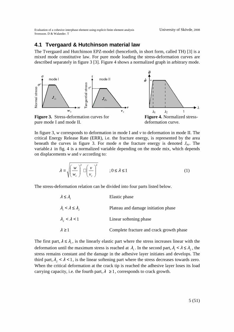
4.1 Tvergaard & Hutchinson material law The Tvergaard and Hutchinson EPZ-model (henceforth, in short form, called TH) [3] is a mixed mode constitutive law. For pure mode loading the stress-deformation curves are described separately in figure 3 [3]. Figure 4 shows a normalized graph in arbitrary mode.
Figure 3. Stress-deformation curves for pure mode I and mode II.
Figure 4. Normalized stress-deformation curve.
In figure 3, w corresponds to deformation in mode I and v to deformation in mode II. The critical Energy Release Rate (ERR), i.e. the fracture energy, is represented by the area beneath the curves in figure 3. For mode n the fracture energy is denoted Jnc. The variableλ in fig. 4 is a normalized variable depending on the mode mix, which depends on displacements w and v according to:
22
+
=
cc v
v
w
wλ ; 10 ≤≤ λ (1)
The stress-deformation relation can be divided into four parts listed below.
1λλ ≤ Elastic phase
21 λλλ ≤< Plateau and damage initiation phase
12 << λλ Linear softening phase
1≥λ Complete fracture and crack growth phase The first part, 1λλ ≤ , is the linearly elastic part where the stress increases linear with the
deformation until the maximum stress is reached at 1λ . In the second part, 21 λλλ ≤< , the stress remains constant and the damage in the adhesive layer initiates and develops. The third part, 12 << λλ , is the linear softening part where the stress decreases towards zero. When the critical deformation at the crack tip is reached the adhesive layer loses its load carrying capacity, i.e. the fourth part, 1≥λ , corresponds to crack growth.
Evaluation of a cohesive interphase element using explicit finite element analysis University of Skövde, 2008 Svensson. D & Walander. T
6 (51)
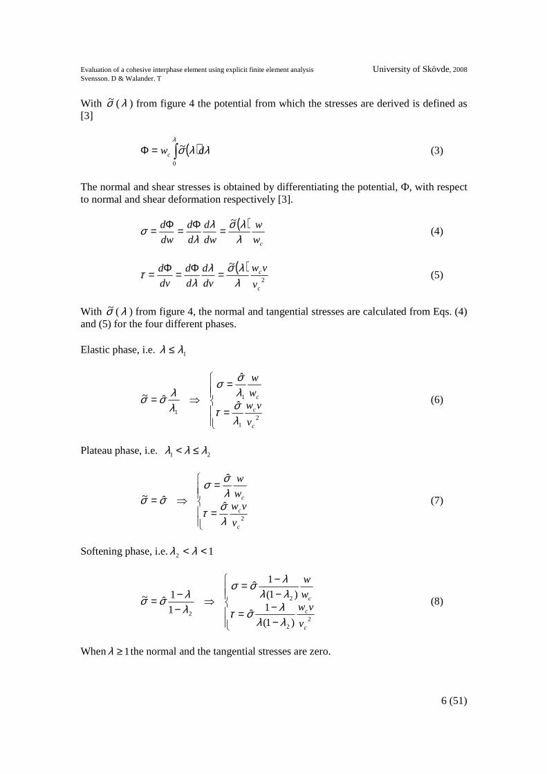
With σ~ ( λ ) from figure 4 the potential from which the stresses are derived is defined as [3]
( )∫=Φλ
λλσ0
~ dwc (3)
The normal and shear stresses is obtained by differentiating the potential, Ф, with respect to normal and shear deformation respectively [3].
( )cw
w
dw
d
d
d
dw
d
λλσλ
λσ
~=Φ=Φ= (4)
( )
2
~
c
c
v
vw
dv
d
d
d
dv
d
λλσλ
λτ =Φ=Φ= (5)
With σ~ ( λ ) from figure 4, the normal and tangential stresses are calculated from Eqs. (4) and (5) for the four different phases. Elastic phase, i.e. 1λλ ≤
=
=⇒=
21
1
1ˆ
ˆ
ˆ~
c
c
c
v
vww
w
λστ
λσσ
λλσσ (6)
Plateau phase, i.e. 21 λλλ ≤<
=
=⇒=
2
ˆ
ˆ
ˆ~
c
c
c
v
vww
w
λστ
λσσ
σσ (7)
Softening phase, i.e. 12 << λλ
−−=
−−=
⇒−−=
22
2
2
)1(
1ˆ
)1(
1ˆ
1
1ˆ~
c
c
c
v
vww
w
λλλστ
λλλσσ
λλσσ (8)
When 1≥λ the normal and the tangential stresses are zero.

Evaluation of a cohesive interphase element using explicit finite element analysis University of Skövde, 2008 Svensson. D & Walander. T
7 (51)
5. User element description Commercial finite element programs, e.g. Abaqus, provide a number of constitutive laws in order to calculate the behavior of adhesively joined structures. Those are based on different constitutive relations, e.g. the Benzeggagh-Kenane-material law but no material models based on a TH model is implemented in the commercial software. The interphase element connects to two shell elements at its midplanes, see figure 5.
Figure 5. Left: Adhesive joint. Right: FE-model of the joint with the interphase element. The user element has eight nodes with six degrees of freedom at each node to enable moment calculations in the element. Each node has three translational- and three rotational degrees of freedom, see figure 6.
Figure 6. Degrees of freedom for the user element. Left: translational DOFs. Right: rotational (drilling) DOFs. The numbers are the local DOFs.
5.1 Structure of the element The loading can be described in three steps, on linear step, one plateau step and one linear softening step. These steps are derived from the Tvergaard & Hutchinson material model, see previous chapter. When the element is totally broken the force is zero. The elements are not removed although they have been broken. The fractured element is at this stage unable to withstand any forces that are subjected to it. The procedure in the user-element subroutine can be described in five steps that are briefly described below. These steps are repeated for every time step. The total number of

Evaluation of a cohesive interphase element using explicit finite element analysis University of Skövde, 2008 Svensson. D & Walander. T
8 (51)
time steps is given by equation (9) where Tl is the simulated time and ∆t is the time step increment that is further explained in chapter nine.
t
Tn l
steps ∆= (9)
1. From Abaqus a global displacement vector is given including all of the
displacements for the user elements. In order to obtain this vector it has to be asked for in Abaqus using the “user element” command [4].
2. In this step the global displacement vector given from Abaqus is transformed into
a, for every user element, local displacement vector by multiplying the global vector with a transformation matrix using the geometry of the connected shell elements. Also the rotational degrees of freedom are calculated to be included in the local x-, y- , and z-deformations. Another denotation for those x- y and z-degrees of freedom is to call them local degree of freedom one, two and three. The same proceeding leads to call the rotational degree of freedom around the local x- y- and z-axis for local degree of freedom four, five and six, see figure 6. The shell elements have their nodes in the shell midplane, see figure 7a. Since the deformations in the rotational axis are, from Abaqus, given in units of radians the additional local x-, y-, and z-deformations can be given by trigonometrical relations. For example the local degree of freedom one has by figure 7c contribution of the rotation about the y-axis, see fig.8. Note that rotation about the z-axis does not contribute to the x- y- or z-deformations. The final local deformation is derived by trigonometric relations and is given in equation (10). In this case the deformations are called n∆ where n is represented by the local degree of freedom that can vary from one to three.
Figure 7. a) Nodes directed in the shell midface by Abaqus standard b) Offset nodes in the FORTRAN-code c) Illustration of the rotational contribution in the shell elements.

Evaluation of a cohesive interphase element using explicit finite element analysis University of Skövde, 2008 Svensson. D & Walander. T
9 (51)
Figure 8. Enlargement and further explanation of figure 7c.
In figure 8, dx and dz stands for the contribution from the local rotational degree of freedom five and can be found in equation (10a) term two and equation (10c) term three. The upper node in the figure is represented by the unmoved node shown in figure 7a, the lower left node is represented by the non-offset node from the local rotational axis six and the right node represents the deformed node from local axis six.
)sin(2 511 ∆−∆=∆ H
(10a)
)sin(2 422 ∆+∆=∆ H
(10b)
( ) ( )[ ])cos(1)cos(12 5433 ∆−+∆−+∆=∆ H
(10c)
For small deformations:
5112
∆−∆=∆ H (10d)
4222
∆+∆=∆ H (10e)
33 ∆=∆ (10f)
In equations (10a-f) the first term in the right hand side expression is the translational displacements and the last parts is the contribution from the rotational axis.
3. The local deformations are multiplied with a stiffness parameter in order to get
the stresses. The stiffness is determined from the TH-model. The stiffness is controlled by an if-statement that is divided into four conditions with the variable λ and w, see chapter 4.1, and is able to deal with loading and unloading. When a damaged structure is unloaded the traction decreases to zero with a reduced stiffness. When the damaged structure is reloaded the traction increases with the same reduced stiffness.

Evaluation of a cohesive interphase element using explicit finite element analysis University of Skövde, 2008 Svensson. D & Walander. T
10 (51)
In this step, nodal masses also are applied in the systems derived from the geometry and density of the interphase element. Since the analyses are performed in the explicit mode, the masses results in mass inertia that together with accelerations results in forces. A node gets mass contribution from every element that it is connecting to and by using the shape functions the mass distribution can be portioned correctly to every concerned node. In the code the mass contribution from the interphase element is neglected.
4. The purpose with the stress determination is that it enables calculation of the local
nodal forces. Those can be calculated by multiplying the stresses with the element face area. To enable the element area calculation, a Jacobian determinant has to be used in the scaling process. Fortunately a Jacobian determinant has been calculated simultaneously together with the shape functions in the global-into-local transformation step and this can therefore be used. The area in this case is the particular element size in the concerned direction.
5. The local forces are transformed into Abaqus global system by multiplication
with the transpose of the same transformation matrix in that are used in step two. Abaqus does then recalculate the finite element code and determines, among others, the stresses and displacements in the Abaqus elements. After this, the five step procedure is repeated until all time steps are calculated.
5.2 Multi-processor analyses The computer development is increasing rapidly. Today’s computers have multi-core processors and mother boards that supports more than one processor slot. A great advantage with multi-cores and multi-processors is that the runtime, i.e. the time for the analysis to complete, can be decreased. Abaqus version 6.7 supports multi-processor analyses for its own elements but when user elements are used in the simulation a few inconveniences appears. It is noticed that if a structure is simulated using n numbers of CPUs (Central Processing Unit) the elements in a structure will be divided into just that many pieces as the number, n. Problems will emerge if the number of elements is not equally divided with the number n. When the simulation is performed with only the standard elements this is not a problem. However, when simulations are performed with the user element using the VUEL subroutine, this issue has to be considered. If an inappropriate number of CPUs is chosen, the simulation can be completed with errors. A DCB specimen, cf. chapter 7, consists of two adherends which are partially joined by an adhesive layer. The part of the adherends which are not joined is considered a crack. When modeling the specimen with the Abaqus version 6.7’s own cohesive elements it is allowed to simply leave out the cohesive elements at the crack. However if the adhesive layer is modeled with user elements this is not possible. This is probably a bug in the present version of Abaqus. Instead the adhesive layer has to be distributed over the whole surface between the adherends and in VUEL code extinguish the cohesive elements at the crack by assigning their forces to zero.
Evaluation of a cohesive interphase element using explicit finite element analysis University of Skövde, 2008 Svensson. D & Walander. T
11 (51)
The user elements are assigned a number, called kblock, which is generated in Abaqus. This number is of importance to calculate for example the force vectors. These are collected in a local vector in the VUEL subroutine. The maximum kblock number that can be assigned to a user element is 136. It does not matter what element number the user element is given in Abaqus; in the subroutine they are sorted in a sequence beginning with one. To perform, for example, a DCB simulation a loop over kblock is used. The loop is using kblock to decide whether an interphase element is located at the crack and if so the force within that element is set to zero. Using kblock is unfortunately not error free. An easy way of modeling with this error in mind is to have exactly 136 elements in length-direction or less than 136 user elements in the simulated structure. If neither of these methods is used the crack will be dislocated. However this is a very limited way of modeling the specimen. To solve this problem another vector in the subroutine code can be used. This vector deals with the global element numbers instead of kblock and with this global vector the former limit of 136 user elements disappears. However the number of elements on a length-row must be equally dividable with the number of CPUs that are used. A safe way to deal with this is to always have one operating processor but this leads to unnecessary long runtimes.
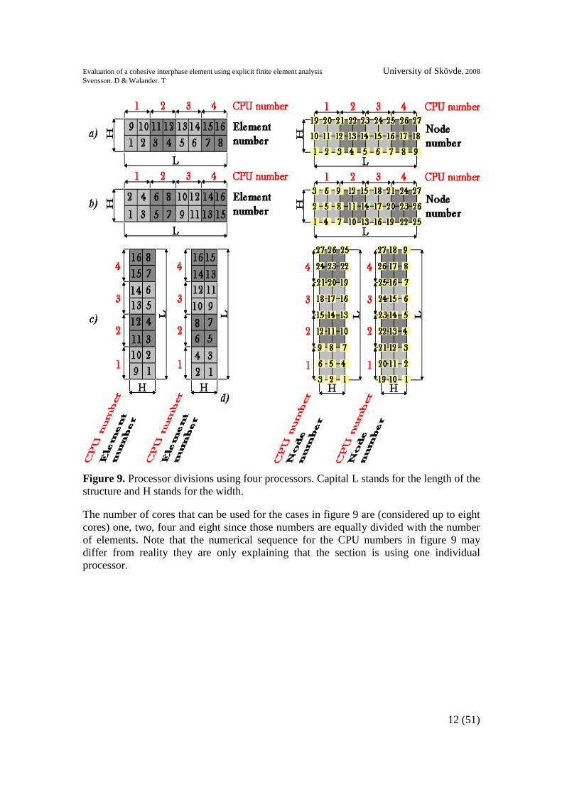
5.2.1 Processor division An important issue when more then one processor is used in combination with user elements is how the elements are divided to each processor. Several tests have proved that when a long and narrow specimen is used, e.g. a DCB-specimen, the specimen is divided in length-direction independent of element numbers, node numbers and also in which direction the specimen are modeled in. This is further explained in figure 9. All CPUs must be assigned the same number of elements, or else the analysis will fail. The failure occurs due to misplaced user elements, i.e. the force within an element at the crack is not zero. This leads to unsymmetrical stresses with respect to the width of the specimen. Another issue is that when more then one user performs analyses on the same CPU that are already used; the element division will be interrupted and the analysis will complete with errors. If more than one analysis is to be executed there are two ways to solve this. The first solution is to halve the numbers of operating processors e.g. from eight to four. Then two analyses can be executed at the same time. The other way to solve this problem is to change the queue order at the computer so only one analysis is performed at the same time. The queued analysis will automatically start immediately after the first analysis is finished.
Evaluation of a cohesive interphase element using explicit finite element analysis University of Skövde, 2008 Svensson. D & Walander. T
12 (51)
Figure 9. Processor divisions using four processors. Capital L stands for the length of the structure and H stands for the width. The number of cores that can be used for the cases in figure 9 are (considered up to eight cores) one, two, four and eight since those numbers are equally divided with the number of elements. Note that the numerical sequence for the CPU numbers in figure 9 may differ from reality they are only explaining that the section is using one individual processor.

Evaluation of a cohesive interphase element using explicit finite element analysis University of Skövde, 2008 Svensson. D & Walander. T
13 (51)
6. Evaluation of the interphase element Before testing the element in a full scale model, the behavior of it is first analyzed using a simple model. The simplest scenario possible is modeled using one user element between two shell elements. The bottom shell nodes are fixed in all translational and rotational displacements. This will lead to a slightly higher effective Young’s modulus of the adhesive layer because of the constraints.
Figure 10. Peel loading
Figure 11. Shear loading
Figure 12. Mixed-mode loading
The structure is tested in the three load cases according to figures 10 to 12. The major purpose with the tests is to validate a TH-behavior. By integrating the stress-deformation curve the total stored energy, i.e. the energy release rate in the system can be calculated. In all the tests, the displacement of the free nodes is prescribed in the directions represented by the arrows in the figures. The displacements are large enough to fracture the adhesive layer. The reaction forces and the displacements in the upper nodes are measured during the simulation. Since the model is simulated in explicit mode the applying loads must be applied slow enough to avoid influence of mass inertia. This is avoided by using a smooth δ(t) curve, see figure 13, which results in very small inertia-forces. The Greek letter ∆ denotes the deformation of the nodes and Tl denotes the simulation time. The acceleration is given by the second differentiation of the curve.
Figure 13. Curve for minimum acceleration-force contribution [4] The elements have the same material properties in all three tests. Material properties used in the tests are presented in table 1. Nodes of the lower shell are fixed in all three tests.

Evaluation of a cohesive interphase element using explicit finite element analysis University of Skövde, 2008 Svensson. D & Walander. T
14 (51)
Young’s modulus [GPa]
Adhesive thickness
[mm]
Density adhesive [kg / m3]
Density adherend [kg / m3]
1λ [-]
2λ [-]
cw [µm]
cv [µm]
σ [MPa]
200 0.200 1350 7800 1.0 10-2 3.1 10-2 80 150 20.0
Table 1. Material properties for the adhesive layer. In the tension/peel-test the interphase element fractures at a displacement of 80 µm. To make sure that the adhesive layer fractures, the applied deformation is set to be 100 µm. The simulation time is in this case set to be 10 ms. The prescribed deformation and simulation time leads to an average acceleration of 1 m/s2. This is slow enough to avoid mass inertia forces. The results from the analyses are given in terms of forces and displacements. The stresses are calculated by dividing the forces with the shell face area. The shear test is very similar to the peel test but it differs in the direction of the applied deformations. The critical shear deformation is larger than the critical peel deformation. The adhesive in this case fracture at a deformation of 150 µm. Therefore the applied deformations are increased to 170 µm. The simulation time is set to be 10 ms which leads to an average acceleration of 1.7 m/s2. This is also slow enough to avoid mass inertia forces. In the mixed mode test the prescribed deformations is the same as in the previous tests but now they are applied at the same time. The simulation time is set to be 10 ms.
6.1 Test results All the results are presented below. The images with even numbers shows the stress-deformation curves that is obtained from each simulation. The energy release rates are calculated by integration of the previous stress-deformation curve. The figures that show the energy release rates have odd figure numbers.
Evaluation of a cohesive interphase element using explicit finite element analysis University of Skövde, 2008 Svensson. D & Walander. T
15 (51)
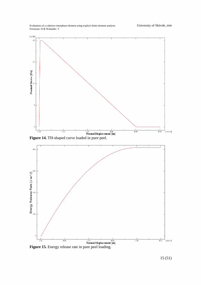
Figure 14. TH-shaped curve loaded in pure peel.
Figure 15. Energy release rate in pure peel loading.
Evaluation of a cohesive interphase element using explicit finite element analysis University of Skövde, 2008 Svensson. D & Walander. T
16 (51)
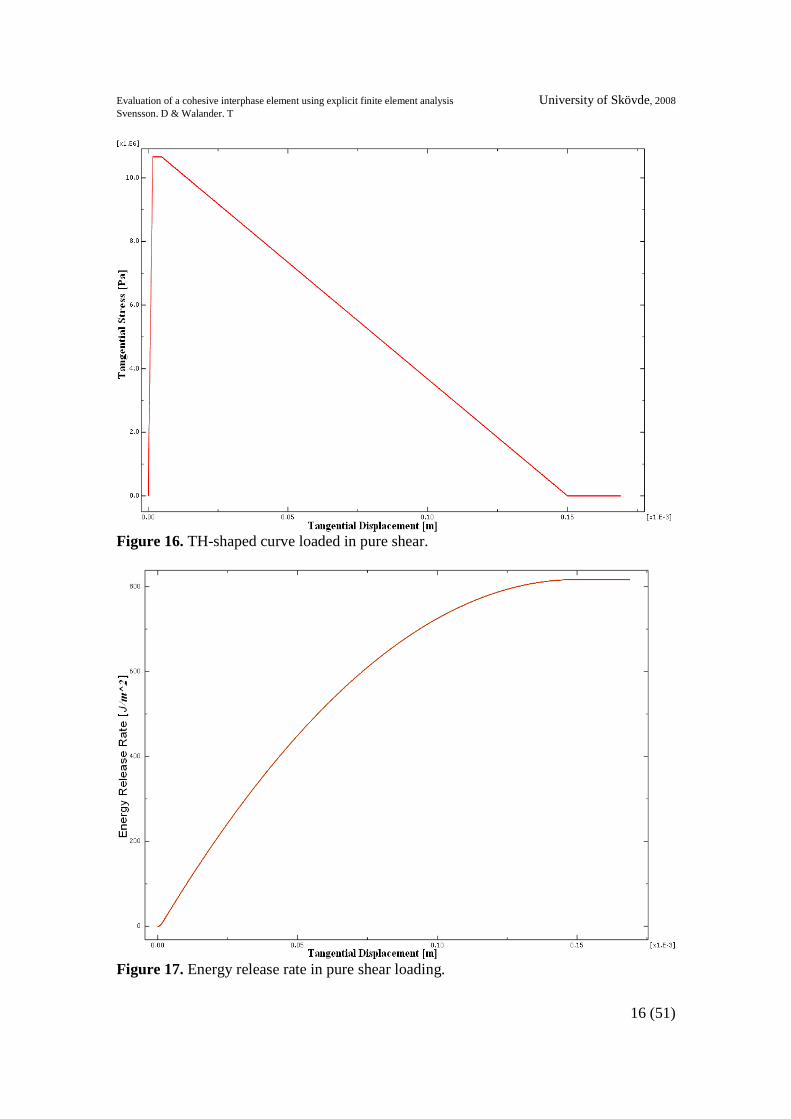
Figure 16. TH-shaped curve loaded in pure shear.
Figure 17. Energy release rate in pure shear loading.

Evaluation of a cohesive interphase element using explicit finite element analysis University of Skövde, 2008 Svensson. D & Walander. T
17 (51)
Figure 18. TH-shaped curve in peel for the Mixed-mode analysis.
Figure 19. Energy release rate in peel for the Mixed-mode analysis.
Evaluation of a cohesive interphase element using explicit finite element analysis University of Skövde, 2008 Svensson. D & Walander. T
18 (51)
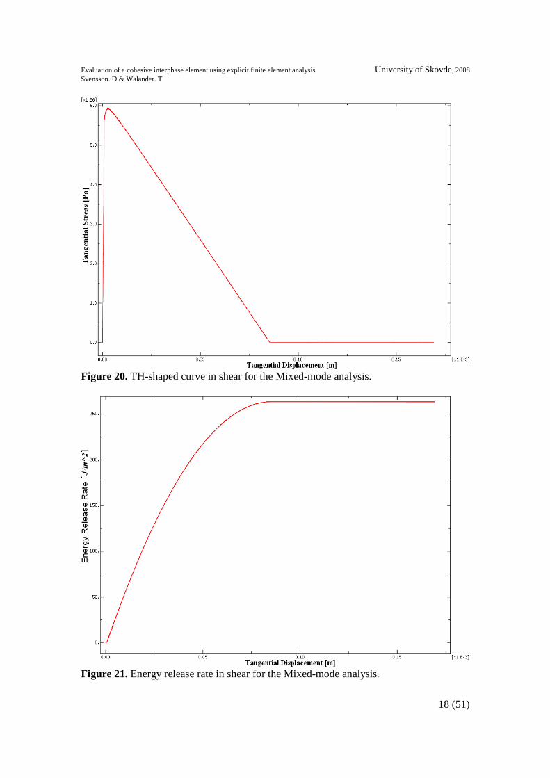
Figure 20. TH-shaped curve in shear for the Mixed-mode analysis.
Figure 21. Energy release rate in shear for the Mixed-mode analysis.

Evaluation of a cohesive interphase element using explicit finite element analysis University of Skövde, 2008 Svensson. D & Walander. T
19 (51)
From figures 14 and 16 it can be observed that the pure peel loaded structure reaches a maximum normal stress of 20 MPa and the pure shear loaded structure reaches maximum shear stress of 10.8 MPa. In booth tests the adhesive fracture energy determined to be 817 J/m2. This value of the fracture energy is expected since the area under the stress-deformation curve is 816.8 for this constitutive relation. Since the critical deformation in mode II is larger than in mode I the critical shear stress must be lower to obtain identical fracture energies. This is also showed in figure 14 and 16 where the peel loaded structure bear for a displacement of 80 µm and the shear loaded structure bear for a displacement of 150 µm. In the Mixed-mode loaded structure a perfect TH-curve is not achieved for any of the loading directions. This is caused because there is no longer a single acting influence of the structure and therefore a perfect TH-curve is not possible to achieve in a single mode. In peel loading the energy release rate exceeds to 553 J/m2which is about 68% of the fracture energy in pure mode loading. The shear loading energy release rate is in mixed-mode 264 J/m2, which is about 32 % of the fracture energy for mode loading. The reason to the larger energy release rate in mode I is that both modes are subjected to equally large deformations and the adhesive have a larger critical deformation in mode II. If the two energy release rate curves in the mixed mode figures 19 and 21 are added together the critical energy release, i.e. the fracture energy is 817 J/m2. These tests shows that the interphase element behaves as expected.

Evaluation of a cohesive interphase element using explicit finite element analysis University of Skövde, 2008 Svensson. D & Walander. T
20 (51)
7. Double Cantilever Beam (DCB)
7.1 Introduction The DCB-specimen consists of two beams, called adherends partially joined by an adhesive layer. The part between the adherends which are not joined together by the adhesive layer is considered as a crack and therefore the start of the adhesive is denoted the crack tip. The edges of the adherends are subjected to two loads F in the vertical direction separating the two adherends. This gives almost pure mode I conditions in the adhesive and therefore the DCB-specimen is very suitable for analyzing the interphase element when loaded in peel. In figure 22 the geometry of the DCB-specimen is displayed. The geometry is symmetric with the symmetry plane in the middle of the adhesive layer. In order to achieve pure mode I conditions the specimen has to be symmetric and the material behavior of the adherends must be identical.
Figure 22. Geometry of the DCB-specimen. Finite element simulations are performed with Abaqus version 6.7 with the interphase elements representing the adhesive layer. The simulations are performed with varying geometry of the specimen and constitutive properties of the interphase element. The results are compared to the analytical solutions obtained by using the equations (11) and (12) discussed in subchapter 7.2. Simulations are also performed with distorted element meshes and the results are compared to the simulations performed with non-distorted elements.
7.2 Basic theory There is no method to directly determine the peel stress at the crack tip for a DCB-specimen. An indirect method has to be used for calculation of the peel stress. The method is to measure the applied energy release rate. The relation between the energy release rate and peel stress is well known, thus it is possible to determine the peel stress. The calculation of the energy release rate is used to predict fracture in the adhesive layer. When the energy release rate reaches its critical limit, i.e. the fracture energy of the adhesive, the adhesive layer loses its load carrying capacity and a crack starts to propagate. For a DCB-specimen the energy release rate is given by [5],
( )b
FdwwJ
)sin(2 θσ == ∫ (11)
Evaluation of a cohesive interphase element using explicit finite element analysis University of Skövde, 2008 Svensson. D & Walander. T
21 (51)
where F is the applied load, θ the rotational displacement at the loading point, w is the elongation of the adhesive at the crack tip and b is the width of the specimen. In Eq. (11) the force is multiplied by 2 since there are two forces acting on the specimen. For details of the derivation, cf. [6]. Differentiation of Eq. (11) yields the constitutive relation, i.e. the stress-deformation relation, for the adhesive at the crack tip,
=b
F
dw
dw
θσ 2)( (12)
Eq. (11) and (12) are used to analyze and validate the results of the simulations.
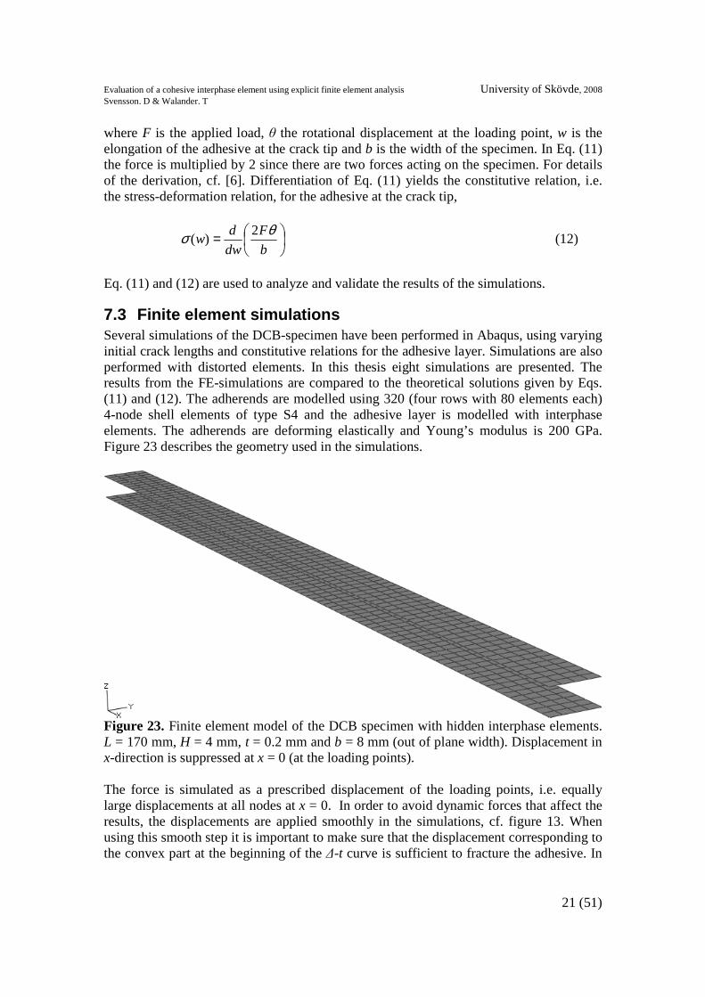
7.3 Finite element simulations Several simulations of the DCB-specimen have been performed in Abaqus, using varying initial crack lengths and constitutive relations for the adhesive layer. Simulations are also performed with distorted elements. In this thesis eight simulations are presented. The results from the FE-simulations are compared to the theoretical solutions given by Eqs. (11) and (12). The adherends are modelled using 320 (four rows with 80 elements each) 4-node shell elements of type S4 and the adhesive layer is modelled with interphase elements. The adherends are deforming elastically and Young’s modulus is 200 GPa. Figure 23 describes the geometry used in the simulations.
Figure 23. Finite element model of the DCB specimen with hidden interphase elements. L = 170 mm, H = 4 mm, t = 0.2 mm and b = 8 mm (out of plane width). Displacement in x-direction is suppressed at x = 0 (at the loading points). The force is simulated as a prescribed displacement of the loading points, i.e. equally large displacements at all nodes at x = 0. In order to avoid dynamic forces that affect the results, the displacements are applied smoothly in the simulations, cf. figure 13. When using this smooth step it is important to make sure that the displacement corresponding to the convex part at the beginning of the ∆-t curve is sufficient to fracture the adhesive. In

Evaluation of a cohesive interphase element using explicit finite element analysis University of Skövde, 2008 Svensson. D & Walander. T
22 (51)
that way the acceleration of the displacement and dynamic forces are kept at the minimum. The height-width ratio used in the simulations is large enough to avoid anti-clastic bending, i.e. the deflection does not vary with respect to the y-axis [7].
7.4 Constitutive behavior of the adhesive layer The constitutive behaviour of the interphase element is described as a simplified σ-w, i.e. stress-elongation, relation according to Tvergaard and Hutchinson cohesive law, cf. Chapter 1. The constitutive relation is determined by the parameters σc, w1 ,w2 and wc, where w denotes the elongation and σ the peel stress of the adhesive at the crack tip. The subscripted c denotes critical. These parameters are shown in figure 24.
Figure 24. σ- w relation for the cohesive user element loaded in peel. Three different σ-w relations have been used in the DCB-simulations. The specimens have the geometry described in figure 23 and the initial crack length is 0.25L. All simulations have the same critical peel stress and critical elongation, with different values on w1 and w2. Adjusting these parameters obviously changes for example the elastic stiffness and the fracture energy since the total area under the σ(w) curve corresponds to the fracture energy. The fracture energy is the maximum value of the energy release rate which occurs when the elongation has reached its critical value. The input data for the constitutive behaviour in the three simulations are shown in table 3.
Simulation Critical peel stress
[MPa] wc
[µm] w1
[µm] w2
[µm] 1 20 80 0.8 2.4 2 20 80 2.4 2.4 3 20 80 0.8 0.8
Table 2. Input data for the constitutive relations A comparison has been made of the theoretical curve of the energy release rate as a function of the elongation of the adhesive at the crack tip, i.e. the J(w) curve, and the same, from the FE-simulations. To create the theoretical σ(w) curve and also integrate the same a program has been made in MATLAB. The input data for this program is the parameters in table 3. The theoretical J(w) curve is obtained by numerically integrating the σ(w) curve using a large number of intervals. For the curve from the FE-

Evaluation of a cohesive interphase element using explicit finite element analysis University of Skövde, 2008 Svensson. D & Walander. T
23 (51)
simulations Eq. (11) has been used. When calculating the energy release rate with Eq. (12) no constitutive relation needs to be known. The results of the comparison are shown in figure 25.
Figure 25. Result of the simulation. Left: Constitutive relations used in the simulations. Right: The energy release rate as a function of the elongation. Solid lines correspond to the integrated curves. Dashed lines correspond to the result from the simulation. Figure 25 shows very good agreement between the analytical curves and the results from the simulations. The curve for simulation 1 shows a somewhat better agreement than the

Evaluation of a cohesive interphase element using explicit finite element analysis University of Skövde, 2008 Svensson. D & Walander. T
24 (51)
curves from simulation 2 and 3. For this geometry the agreement between the simulation and the analytical results is excellent when using a plateau part in the σ-w relation. When using a sawtooth model, i.e. w1 = w2, the curves slightly diverges at the end and the fracture energy from the simulations are somewhat too large. However the fracture energy from the simulations is diverging less than 2 % and the agreement is considered good. In addition to the simulations described above three more simulations are performed with different values of the initial crack lengths. In these simulations the σ-w relation of simulation 1 is used. The J(w) curves from the simulations are compared to the analytical J(w) curves. The result of the comparison is shown in figure 26.
Figure 26. J(w) curves from the DCB-simulations with different initial crack lengths. Solid lines corresponds to the analytical J(w) curves. Dashed lines corresponds to the J(w) curves from the simulations.
Figure 26 shows a fairly good agreement between the analytical curves and the curve from the simulations. The fracture energy from the simulations is the same as the analytical fracture energy. All attempts to achieve a better agreement have failed when using an initial crack length of 0.1L or 0.2L. The reason is believed to be that the length of the adherends which are not joined together is too short for Eq. (11) to be accurate. Eq. (11) are based on beam theory, therefore the part of the adherends which are not
Evaluation of a cohesive interphase element using explicit finite element analysis University of Skövde, 2008 Svensson. D & Walander. T
25 (51)
joined together has to be long enough to be considered as beams. Several tests with varying geometry of the specimen agree with this conclusion.
The bottom right of figure 26 shows the comparison performed with a specimen that is twice as long, i.e. L = 340 mm, and with this geometry the curves are coinciding. When using an initial crack length of 0.3L or longer the geometry of the specimen described in figure 23 is not long enough. According to the simulations the adhesive at x = L is subjected to peel stress when using L = 170 mm, i.e. the adhesive layer is too short.
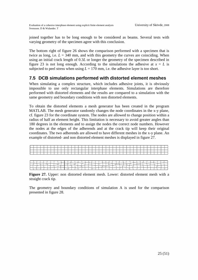
7.5 DCB simulations performed with distorted element meshes When simulating a complex structure, which includes adhesive joints, it is obviously impossible to use only rectangular interphase elements. Simulations are therefore performed with distorted elements and the results are compared to a simulation with the same geometry and boundary conditions with non distorted elements. To obtain the distorted elements a mesh generator has been created in the program MATLAB. The mesh generator randomly changes the node coordinates in the x-y plane, cf. figure 23 for the coordinate system. The nodes are allowed to change position within a radius of half an element height. This limitation is necessary to avoid greater angles than 180 degrees in the elements and to assign the nodes the correct node numbers. However the nodes at the edges of the adherends and at the crack tip will keep their original coordinates. The two adherends are allowed to have different meshes in the x-y plane. An example of distorted- and non distorted element meshes is displayed in figure 27.
Figure 27. Upper: non distorted element mesh. Lower: distorted element mesh with a straight crack tip. The geometry and boundary conditions of simulation A is used for the comparison presented in figure 28.

Evaluation of a cohesive interphase element using explicit finite element analysis University of Skövde, 2008 Svensson. D & Walander. T
26 (51)
Figure 28. Applied load vs. deflection at the loading points. The dashed line corresponds to the simulation performed with distorted elements. Solid line corresponds to the simulation performed with non distorted elements. Figure 28 shows an excellent agreement of the curves. In figure 29 the stress distributions from the simulations are visualized
Figure 29. Stress distribution from simulations with distorted and non distorted elements.
Figure 29 also shows an excellent agreement of the stress distributions. This indicates that distorted elements can be used without reducing the accuracy of the results when simulating the DCB-specimen. Several simulations have been made with varying geometries and different mesh generations; all results are supporting this conclusion.

Evaluation of a cohesive interphase element using explicit finite element analysis University of Skövde, 2008 Svensson. D & Walander. T
27 (51)
8. End Notch Flexure (ENF)
8.1 Introduction The end-notch flexure-specimen (ENF-specimen) is commonly used for shear testing of adhesive joints. The ENF-specimen consists of two adherends joined together by an adhesive layer. The adhesive layer is shorter than the adherends. The part of the adherends which are not joined is considered a crack, thus the start of the adhesive layer is considered the crack tip. The bottom adherend is placed on two rigid supports and a load is applied on the upper adherend symmetrically between the two supports. This geometry and boundary conditions gives almost pure mode II conditions at the crack tip and the ENF-specimen is very suitable for shear testing of an adhesive layer. The geometry of a ENF-specimen is displayed in figure 30.
Figure 30. Geometry of the ENF-specimen, the geometry is defined by the length between the supports L, the height of the adherends H, and the crack length a.
8.2 Basic theory There is no known way to directly determine the shear stress acting at the crack tip when simulating or performing experiments with the ENF-specimen. Thus, an indirect method has to be used. The method is to calculate the energy release rate and the shear deformation of the adhesive layer. Then the shear stress acting on the crack tip can be determined. In [8] an equation is derived for the energy release rate.
32
22
016
9
HEW
aPJ = (13)
This formula gives the energy release rate for a rigid adhesive layer, i.e. it does not account for the flexibility of the adhesive layer and therefore it is an underestimation of the fracture energy. An equation that does account for the flexibility has been derived by Alfredsson [9].
22
2
32
20
2
0 128
9
8
3
16
9)()(
HkW
P
WH
vP
HEW
aPdvvvJ
v
−+≈= ∫τ (14)

Evaluation of a cohesive interphase element using explicit finite element analysis University of Skövde, 2008 Svensson. D & Walander. T
28 (51)
Here v is the shear deformation at the crack tip, E is Young modulus of the adherends, W the width of the adherends and k is the initial stiffness of the adhesive layer. Since the third term is very small compared to the other terms it is neglected in this work. Eq. (14) is only valid if the adherends deform elastically and before the crack have propagated past the loading point. Differentiation of Eq. (14) gives the constitutive stress-deformation relation.
dv
vdJv
)()( =τ (15)
Eq. (14) is used for approximately determination of the critical applied load. This is done by simply putting J=Jc
and v= vc and solving for P=Pc [9].
)11
13 22
2
−
+=
γa
vEWHP c
c where a
v
J
EH c
c4
1=γ
(16)
The equations stated above are sufficient to obtain and analyze the results from the simulations.
8.3 FE-simulation of the ENF-specimen Simulations of the ENF-specimen have been made in Abaqus version 6.7. The results from the FE-simulations are compared to a theoretical solution given by the constitutive relation. In this thesis all simulations of the ENF-specimen have the geometry and boundary conditions described in figure 30. This is to fulfil the stability conditions, i.e. where the crack has to be long enough and also have a long enough distance between the crack tip and the loading point. The adherends are deforming elastically which is a criterion for Eq. (14) to be valid. Young’s modulus for the adherends is 200 GPa in all simulations.

Evaluation of a cohesive interphase element using explicit finite element analysis University of Skövde, 2008 Svensson. D & Walander. T
29 (51)
Figure 31. Finite element model of the ENF specimen with hidden user elements. Dimensions used in simulations are H = W = 16 mm, L = 1000 mm, t = 0.2 mm, a = 375 mm (W = out of plane width, t = adhesive thickness). The adherends are modelled using 4-node shell elements of type S4 and the adhesive layer is modelled with cohesive user elements. In the simulations discussed in this work each adherend is modelled with 320 (four rows of 80 elements each) shell elements and the adhesive layer are modelled with 200 (four rows of 50 elements each) interphase elements. Displacement in z-direction of the lower adherend are suppressed at x = 0 and x = L. Displacement in the x-direction of the lower adherend are also suppressed at x = L. Several simulations show that this mesh is reasonable since fewer elements give less accurate results and more elements gives longer runtimes without substantially increasing the accuracy of the results. The applied load is simulated as a prescribed deflection at the loading point. For calculation of the critical deflection at the loading point Eq. (17) is used. This is an underestimation of the critical deflection since it is based on linear elastic fracture mechanics (LEFM), and does not account for the flexibility of the adhesive [9].
( )333
1232
1La
EWH
Pc +=∆ (17)
In the simulations the largest deflection is 8 mm which is half the height of the adherends. When using Eq. (14) to calculate the energy release rate J, only two parameters needs to be determined from the simulation, namely the applied load and the shear deformation at the crack tip. The remaining terms in the equation are geometry- and material constants. The applied load is obtained by simply requesting it as output data in the FE-software and the shear deformation is calculated by using Eq. (18), derived by Alfredsson [10].
Evaluation of a cohesive interphase element using explicit finite element analysis University of Skövde, 2008 Svensson. D & Walander. T
30 (51)
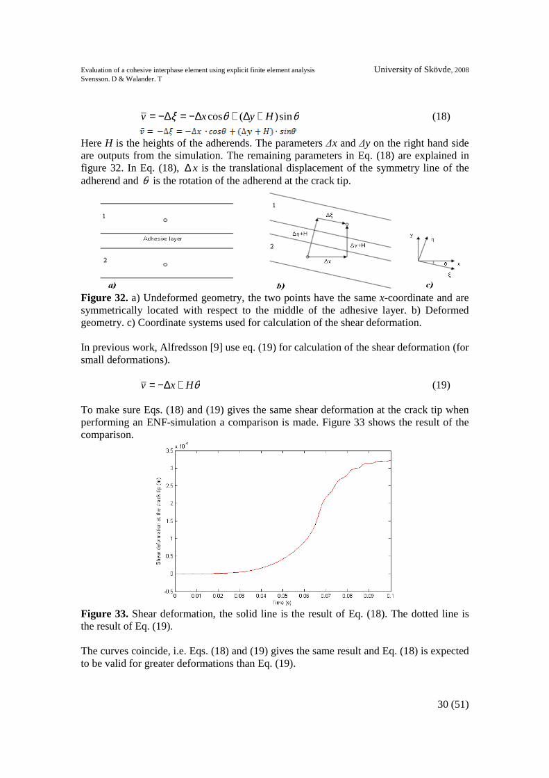
θθξ sin)(cos Hyxv +∆+∆−=∆−= (18)
Here H is the heights of the adherends. The parameters ∆x and ∆y on the right hand side are outputs from the simulation. The remaining parameters in Eq. (18) are explained in figure 32. In Eq. (18), ∆ x is the translational displacement of the symmetry line of the adherend and θ is the rotation of the adherend at the crack tip.
Figure 32. a) Undeformed geometry, the two points have the same x-coordinate and are symmetrically located with respect to the middle of the adhesive layer. b) Deformed geometry. c) Coordinate systems used for calculation of the shear deformation. In previous work, Alfredsson [9] use eq. (19) for calculation of the shear deformation (for small deformations).
θHxv +∆−= (19) To make sure Eqs. (18) and (19) gives the same shear deformation at the crack tip when performing an ENF-simulation a comparison is made. Figure 33 shows the result of the comparison.
Figure 33. Shear deformation, the solid line is the result of Eq. (18). The dotted line is the result of Eq. (19). The curves coincide, i.e. Eqs. (18) and (19) gives the same result and Eq. (18) is expected to be valid for greater deformations than Eq. (19).
Evaluation of a cohesive interphase element using explicit finite element analysis University of Skövde, 2008 Svensson. D & Walander. T
31 (51)
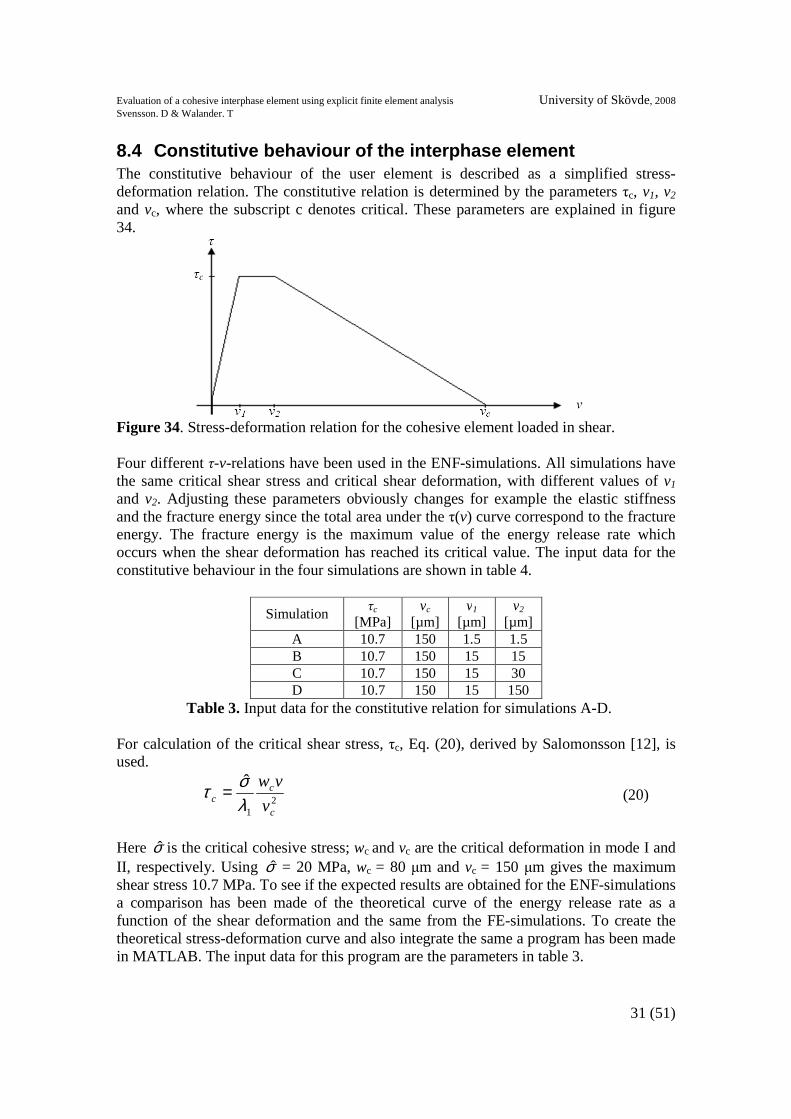
8.4 Constitutive behaviour of the interphase element The constitutive behaviour of the user element is described as a simplified stress-deformation relation. The constitutive relation is determined by the parameters τc, v1, v2 and vc, where the subscript c denotes critical. These parameters are explained in figure 34.
Figure 34. Stress-deformation relation for the cohesive element loaded in shear. Four different τ-v-relations have been used in the ENF-simulations. All simulations have the same critical shear stress and critical shear deformation, with different values of v1 and v2. Adjusting these parameters obviously changes for example the elastic stiffness and the fracture energy since the total area under the τ(v) curve correspond to the fracture energy. The fracture energy is the maximum value of the energy release rate which occurs when the shear deformation has reached its critical value. The input data for the constitutive behaviour in the four simulations are shown in table 4.
Simulation τc
[MPa] vc
[µm] v1
[µm] v2
[µm] A 10.7 150 1.5 1.5 B 10.7 150 15 15 C 10.7 150 15 30 D 10.7 150 15 150
Table 3. Input data for the constitutive relation for simulations A-D. For calculation of the critical shear stress, τc, Eq. (20), derived by Salomonsson [12], is used.
21
ˆ
c
cc v
vw
λστ = (20)
Here σ̂ is the critical cohesive stress; wc and vc are the critical deformation in mode I and II, respectively. Using σ̂ = 20 MPa, wc = 80 µm and vc = 150 µm gives the maximum shear stress 10.7 MPa. To see if the expected results are obtained for the ENF-simulations a comparison has been made of the theoretical curve of the energy release rate as a function of the shear deformation and the same from the FE-simulations. To create the theoretical stress-deformation curve and also integrate the same a program has been made in MATLAB. The input data for this program are the parameters in table 3.

Evaluation of a cohesive interphase element using explicit finite element analysis University of Skövde, 2008 Svensson. D & Walander. T
32 (51)
The theoretical J(v) curve is obtained by numerically integrating the τ(v) curve according to Eq. (15) with a large number of intervals. For the curve from the FE-simulations Eq. (14) has been used. When calculating the energy release rate with Eq. (14) no constitutive relations need to be known. The results of this comparison are displayed in figure 35.

Evaluation of a cohesive interphase element using explicit finite element analysis University of Skövde, 2008 Svensson. D & Walander. T
33 (51)
Figure 35. On the left side, the constitutive relation is described. On the right side the dashed curves correspond to the integration of the curves on the left. The solid lines are the J(v) curve obtained from simulations using Eq. (14).

Evaluation of a cohesive interphase element using explicit finite element analysis University of Skövde, 2008 Svensson. D & Walander. T
34 (51)
Figure 35 show very good agreement of the energy release rate for the analytical model and the result from the FE-simulations. In the FE-simulations when using Eq. (14), the energy release rate should remain constant when the fracture energy is reached but this is not the case since Eq. (14) is not valid when the crack has propagated past the loading point. In simulations A, B and C the crack tip has reached the loading point at approximately v = 220 µm, at this shear deformation the energy release rate are increasing rapidly. In simulation A the elastic stiffness is much greater than the other simulations and the constitutive relation can be considered a sawtooth model. Several simulations show that when using this τ-v- relation and using more than four CPU’s the curves are diverging. The result of the FE-simulation when using more than four CPU’s is a J-curve that corresponds to a simulation with a higher value of v1, i.e. a softer behaviour in the elastic part. This problem does not occur in any other simulations where a higher value of v1, i.e. a smaller value of the elastic stiffness is used. The constitutive relations used in simulation C and D have a plateau part, i.e. the shear stress remains constant at its critical value. This plateau part has been proven to exist by experiments with the ENF-specimen, cf. [6]. In simulation D the adhesive layer have no softening part and loses its load carrying capacity suddenly, this can be considered an ideal plastic adhesive layer. Since the shear stress in simulation D drops from its critical value to zero instantaneously the J-curve does not have the last concave part when the value of J is approaching the fracture energy.
8.5 Stability study of the user cohesive element This chapter handles stability due to the geometry of the specimen. For numerical stability conditions see chapter 9. To capture the complete stress-deformation relation stable crack propagation is necessary. For a rigid adhesive layer the critical initial crack length is about a0 = 0.35L [8]. In case the adhesive layer is not rigid this is an overestimation, and the initial crack length is allowed to be shorter [9]. Here a0 = 0.35L is used as the stability condition. To analyse how Abaqus handle instability for the interface element the geometry in figure 31 is simulated with two different initial crack lengths. The first is too short and does not fulfil the stability condition. The force-deflection curves from FE-simulations are compared to the theoretical solution using LEFM according to Eqs (21)-(26). The curve is divided into three parts, one before and two during crack propagation. Before crack propagation Eqs. (21) and (22) are valid [11]. The critical force and deflection is given by.
cc JEH
a
WP 3
03
4= (21)

Evaluation of a cohesive interphase element using explicit finite element analysis University of Skövde, 2008 Svensson. D & Walander. T
35 (51)
3
330
32
)12(
EWH
LaPc
+=∆ (22)
Where a0 is the initial crack length. At the first part of crack propagation Eqs. (23) and (24) are used [11].
cJEHa
WP 3
3
4= for 20
Laa ≤≤ (23)
3
33
32
)12(
EWH
LaP +=∆ for 20
Laa ≤≤ (24)
At the last part, i.e. when the crack tip has reached the loading point Eqs. (25) and (26) are valid [10].
cJEHaL
WP 3
)(3
4
−= (25)
[ ])(9238
33
3aLLaLa
EWH
P −+−=∆ (26)
Eqs. (21) to (26) are implemented in MATLAB for plotting the theoretical force-deflection curve with two different initial crack lengths. The same geometry with the same initial crack lengths are simulated in Abaqus and the results is compared in fig 36. The used geometry is described in figure 31.
Figure 36. Force-deflection curve for the FE-simulation compared to the theoretical curves. Red dashed lines correspond to the force-deflection curve using LEFM. Solid lines are the simulated force-deflection curves. Left: The stability condition is not fulfilled. The initial crack length is a = 0.25L. Right: The stability condition is fulfilled, here a = 0.375L.

Evaluation of a cohesive interphase element using explicit finite element analysis University of Skövde, 2008 Svensson. D & Walander. T
36 (51)
The theoretical curve and the curve from the FE-simulation are coinciding for deflections smaller than 1.5 mm, for larger values of the deflection the curves diverge. For this comparison the simulated curve corresponds to an adhesive layer with the stress-deformation relation used in simulation A which behaves elastically until the shear deformation reaches 1.5 µm. Plotting shear deformation vs. the deflection of the loading point clearly shows that the damage initiates at the deflection of about 1.5 mm, the curves are in good agreement as long as the simulated adhesive behaves elastically. The maximum force in figure 36 where the stability conditions have been fulfilled occurs at the same shear deformation as the theoretical curve. For the simulation where the stability condition have not been fulfilled the maximum force occurs at the deflection where the tangential line of the theoretical curve are vertical, this occurs at point T, as visualised in figure 36. A MATLAB-program is provided by Alfredsson. The program is plotting the force-deflection curve for an ENF simulation with the flexibility of the adhesive layer is taken into account. Here a sawtooth model is used; see simulation B in table 4. The equations in this program are based on non-linear springs and are valid until the damage zone of the adhesive reaches the loading point. In figure 37 the curves from the MATLAB program is compared to the results of the FE-simulation.
Figure 37. Load vs. deflection of the loading point for the two simulations in figure 36 compared to the theoretical solution from the MATLAB program. The red dashed curves are from the FE-simulations and the blue curves are the theoretical solution based on non-linear springs. The initial crack length, a, on the left is 0.375 m and on the right 0.25 m, i.e. the stability condition is fulfilled in the figure to the left but is not fulfilled in the right figure. Figure 37 shows that the curve from the simulation coincides with the theoretical curve when the flexibility is taken into account. On the left hand side of figure 37 where the initial crack length are longer it is only possible to calculate the force-deflection curve until the crack has propagated 2 mm. Both in figure 36 and 37 the lines corresponding to the FE-simulations are greatly fluctuating when the stability conditions are not fulfilled. This is how Abaqus handles instability where no force equilibrium can be found and the problem becomes of dynamic nature. Simulations show that crack lengths shorter than

Evaluation of a cohesive interphase element using explicit finite element analysis University of Skövde, 2008 Svensson. D & Walander. T
37 (51)
0.3375L are resulting in instability. The accuracy of this result is limited since only one element mesh has been used and additional elements could give a somewhat smaller value of the critical crack length.
8.6 ENF simulations performed with distorted elements A comparison has been made of ENF-simulations meshed with only elements with straight angles versus distorted elements. The mesh generator described in the DCB-chapter has been used to perform ENF-simulations with distorted elements. In addition to the adherend edge nodes and the nodes at the crack tip, the nodes at the loading point also have its original coordinates. Given that the same geometry and boundary conditions as in previously described simulations are used it is expected that the results, in terms of load-deflection are the same. However no reasonable results have been achieved when using distorted elements. Figure 38 shows the result.
Figure 38. Comparison of one analysis with right elements (lower line) and one with distorted elements (upper line). In figure 38 the force-deflection curves diverge greatly for the two cases and this proves that ENF simulation performed with distorted elements is not possible in order to obtain correct results. The reason for this is unknown and is suggested as further work for the research group.
Evaluation of a cohesive interphase element using explicit finite element analysis University of Skövde, 2008 Svensson. D & Walander. T
38 (51)
9. Time step analyses
9.1 Introduction Since explicit finite element software’s is more commonly used in today’s industries when simulating large structures it is not only the accuracy in the calculations that are of importance for the software’s efficiency but also the time for the simulation to be completed, i.e. the runtime. An approximate formula for runtime, Tclock, is given by Eq. (27) [13]. Here K is a constant which depends on the computer power; ndof stands for the number of degrees of freedom (DOF’s) in the model and ∆t stands for the length of the time step that are used in the simulation.
tnKT dofclock ∆
⋅≈ 1 (27)
According to Eq. (27) a short runtime is achieved by using a powerful computer, a low number of DOFs or a long time step. Unfortunately a powerful computer, that is well suited for finite element simulations can cost lots of money and therefore this is not a first-hand-choice to minimize the runtime. Another way of shorten the runtime is to have less degrees of freedom in the model. The drawback with this approach is that decreasing the DOFs leads to a less accurate model. A last attempt would be to increase the time step but this is not always failure free. If a too long time step is used in the simulation the analysis will diverge, i.e. fail. The longest time step that can be used in an explicit finite element simulation is called the critical time step and is denoted ∆tc. The exact critical time step is calculated by solving for the largest eigenvalue of the dynamic stiffness matrix. The calculated value is then inserted in Eq. (29). However the stiffness matrix is never calculated in an explicit FE-analysis. Because of this the critical time step needs to be estimated, this is done differently depending on which element type that is used. In a continuum element, e.g. Abacus’s C3D4, it can be estimated as the time it takes for an elastic wave to pass through the element. This is even called the Courant limit [13] and is given in Eq. (28) where lmin stands for the shortest distance between two nodes in the element and c is the wave speed given as the square root of the Young’s modulus; E, over the density, ρ.
ρEc
l
c
lt minmin ==∆ (28)
However, Eq. (28) is not an estimation that is suited for cohesive elements. Since cohesive elements often are modeled as springs they are unable to transfer elastic waves the way that continuum elements do. Instead the critical time step is calculated by finding the maximum eigenvalue frequency for each cohesive element [13]. The largest value of those frequencies is denoted ωmax and is then inserted in Eq. (29).
Evaluation of a cohesive interphase element using explicit finite element analysis University of Skövde, 2008 Svensson. D & Walander. T
39 (51)
max
2
ω=∆ ct (29)
Where ω for a spring can be calculated with aid of Eq. (30) where kspring is the spring stiffness and mtot is the total element mass that the adhesive element is attached to. ωmax is then obtained by determine the largest value of ω for the entire structure.
tot
spring
m
k2≈ω (30)
In a structure with several element types the critical time step is the shortest critical time step for all elements in the model. This is quite easy understood by considering two critical time steps, one for element type A and one for B. A has a critical time step that is half B’s critical time step. If B’s time step is used in the simulation; elements of type A will not manage to complete the simulation since they demand a time step that is shorter or equal to the half of B’s time step. Therefore the shortest critical time step for the entire structure is always controlling the system. In Abaqus the search for the shortest critical time step is performed “element by element” and is a standard procedure in the “dynamic” command. In order to increase the critical time step and thus decrease the runtime for continuum elements one can use mass scaling. Mass scaling implies that the density is increased for the elements that govern the time step. Mass scaling decreases the runtime but it can also cause problems in the simulations. If a too high scale factor is used the mass scaled elements may lead to abnormal mass inertia forces and as a consequence creates high stresses in the structure. In this thesis mass scaling is not used since the simulated structures are small.
9.2 Governing equations The research group at University of Skövde has developed a yet untested method to calculate the critical time step for a complete test structure using both cohesive- and shell elements [14]. Their method is based on Eq. (30) but differs in some way to calculate the maximum frequency, ωmax. In their model a value, α, is introduced by Eq. (31) and is the quota of Young’s modulus for the adhesive layer and for the adherend.
adhesive
adherend
E
E=α (31)
Young’s modulus for the adhesive layer is often slightly higher than the optimal modulus, E. The higher modulus is called the effective Young’s modulus, and is derived in Eq. (32) [14] where ν is the Poisons ratio for the adhesive.
cn
adhesiveadhesive
hEE
δλσ
ννν
1
ˆ
)1)(21(
)1(=
+−−
= (32)

Evaluation of a cohesive interphase element using explicit finite element analysis University of Skövde, 2008 Svensson. D & Walander. T
40 (51)
With aid of Eqs. (29)-(32) the critical time step is derived from the largest value of ωadhesive and ωadherend. The maximum frequency for the adhesive layer, ωadhesive, is constant independent of the variable α. ωadhesive and ωadherend are given by Eqs. (33a) and (33b) [14].
221
2
hhH
E
adhesiveadherend
adhesiveadhesive ρρ
ω+
= (33a)
)2(
82
Hh
adhesiveadherende
adhesiveadherend
L
E
ρραω
+= (33b)
Eq. (33) is derived by the use Eq. (30). In this derivation the element area is assumed to be square and that is also the case that will be evaluated in this thesis. The maximum frequency for a complete structure is plotted versus α. All material properties are collected from table 1 with an element length, Le, of two millimeters.
Figure 39. α-dependent eigen frequency of the system. The axis units is in forms of [-] and [1/s]. In figure 39 the constant horizontal line corresponds to ωadhesive and the sloping curve corresponds to ωadherend. The frequency that governs the critical time step in the structure is marked with a bold line and is the maximum eigenvalue frequency for the current α. The α-value at the intersection of the curves is denoted αi. The adhesive layer governs the critical time step for α-values smaller than αi. According to Eq. (29) the critical time step of the system is calculated inverse proportional to the maximum eigenvalue frequency, i.e. the bold line shown in figure 39.

Evaluation of a cohesive interphase element using explicit finite element analysis University of Skövde, 2008 Svensson. D & Walander. T
41 (51)
By the use of Eqs (29) and (33a,b) the critical time step in a structure can be calculated as the maximum of Eqs. (34a,b).
adhesive
adhesiveadherendadhesivec E
hHht
22 ρρ +=∆ (34a)
adhesive
Hh
adhesiveadherendeadherendc E
Lt
αρρ
2
)2(2 +=∆ (34b)
Values from table 1 are inserted in Eqs. (34a,b) and the theoretical critical time step is plotted versus α in figure 40. Here the element length is 2 mm. By inserting the values from table 1 in Eq. (32) the effective Young’s modulus is 5 GPa. The value of α must be smaller than 2.5 if the adhesive layer shall govern the critical time step. This corresponds to a Young’s modulus of the adherends of maximum 12.5 GPa. The critical time step is in this case governed by the adherends since Young’s modulus is 200 GPa, i.e. α is 40. The critical time step when α is equal to 40 is 0.39 µs.
Figure 40. Critical time step in the system dependent on α. In order to let the adhesive layer govern the critical time step when using a Young’s modulus of 200 GPa for the adherends the length of the element must be increased. The element length, Le, must be increased from 2 mm to 8 mm. This will result in a critical time step of 1.58 µs when α is equal to 40.
9.3 Accuracy determination The analysis in the previous chapter is a theoretical idea and this chapter aims at investigate if Eq. (34) is applicable in an explicit analysis. If the real critical time step is shorter than the calculated critical time step the analysis will fail. Of course a small

Evaluation of a cohesive interphase element using explicit finite element analysis University of Skövde, 2008 Svensson. D & Walander. T
42 (51)
divergence between the calculated value and the simulated can appear and this is also meant to be investigated and evaluated. The test is divided into two categories, one where the ωadhesive governs the critical time step and one where ωadherend is governing the critical time step. All tests described in this section are performed with the DCB-specimen geometry. The critical time step is evaluated by assuming a lower time step than Eq. (34) gives. The time step is then increased until the analysis fails or completes with errors. The critical time step from simulations is then compared with Eq. (34). What differ the evaluations of the critical time steps for the adhesive versus the adherend is the element length, Le. To make sure the adhesive layer governs the critical time step, the element length, Le, is set to 9 mm. In the previous chapter the minimum element length is calculated to be 8 mm but in order to have margins in the tests, the 9 mm element length is used. This will result in a αi of 50.6 and with values from table 1 a critical time step of 1.583 µs when the adhesive governs the critical time step. The critical time step according to Eq. (34) for this simulation is shown in figure 41.
Figure 41. Critical time step according to Eqs. (34a,b) with Le 9 mm. A note is that the time step for the interphase element is, in the VUEL subroutine code, given manually. If this time step is given a too large value the simulation will fail if the adhesive governs the time step. Abaqus will also suggest a time step but this is only considering its own element types and thus it is not interesting in this evaluation. In Abaqus the time increment of the simulation can be given manually by using “direct user control” in the “dynamic” command. The time step is first set to be the calculated critical time step of 1.582 µs and α is set equal to 40. Since the simulation went through without failing, the time step is increased until the simulation fails at a value between 1.582 ≤ ∆tc < 1.583 µs. This indicates that Eq. (34) corresponds well with Abaqus critical

Evaluation of a cohesive interphase element using explicit finite element analysis University of Skövde, 2008 Svensson. D & Walander. T
43 (51)
time step; within less than one billion part of a second. Noteworthy is that Abaqus is suggesting a time step of 1.147 µs which is much shorter than necessary. A similar strategy is used to investigate the critical time step when the adherends governs the critical time step. The element length is decreased to 2 mm. With values from table 1 the calculated critical time step, according to Eq. (34b), is 0.39 µs. The critical time step in the simulation is in this case 0.34 µs, i.e. Eq. (34b) is optimistic. Abaqus suggests 0.286 µs which is a very conservative time step. The value of αi is also studied. This is done by assuming all of the variables in Eq. (34) as fixed except for the Young’s modulus for the adherends, i.e. a varying α-value. The element length is set to 9 mm and material properties are set according to table 1. This results in a critical time step for the adhesive of 1.58 µs. Young’s modulus, E, for the adherends is set to 260 GPa which results in α-value equal to 52, i.e. the adherends governs the time step. Young’s modulus is then decreased until the critical time step is 1.58 µs, i.e. the adhesive governs the critical time step. According to Eqs. (34a) and (34b) αi is 50, i.e. when the Young´s modulus of the adherends are 250 GPa. However according to the simulations αi
is 35.5, i.e. the simulation fails when the Young’s modulus for the adherends is higher than 177.5 GPa. This indicates that Eq. (34) is not applicable for calculating the critical time step. Several simulations have been performed to study if Eq. (34) is correct. These simulations have been performed with varying values of the parameters in Eq. (34). In all of the tests the critical time step is corresponding very well to the analytical given that the adhesive layer governs the critical time step. Several tests have also been made in order to investigate the adherends critical time step and the value of αi. All tests indicate that the analytical value of αi and critical time step for the adherends is an overestimation. Abaqus suggests a time step that is shorter than necessary in all simulations. This means that the runtime of the simulations can be decreased and this is studied in the next section.
9.4 Failure cause investigation This section refers to determine the failure cause and suggesting a correction of the Eq. (34). The investigation is only referring to results from simulations and no theoretical derivations will be made in order to determine the correct equation. In the previously chapter it is remarked that analysis will fail to complete if a too long time step is used. However this is not always true. Some simulations will complete even if they have failed so the output curve has to be studied. In figure 42 the difference between a failed analysis and a successful analysis is visualized. For the parameter values used in this simulation; the critical time step then is within the range 1.582 µs ≤ ∆tc < 1.583 µs. The large movements of the adherends to the left in figure 42 are due to that the model has too few elements to capture the fracture of the adhesive layer. This has nothing to do with the time step.

Evaluation of a cohesive interphase element using explicit finite element analysis University of Skövde, 2008 Svensson. D & Walander. T
44 (51)
Figure 42. Field output curves from identical simulation using different time steps. Left: Valid curve at ∆t =1.582 µs. Right: Failed curve at ∆t =1.583 µs. Note the difference of the axis scales for the force. Several DCB-specimens are modeled using 7, 8 and 12 mm in quadratic element side length, see table 5. Other parameter values are set according to table 1. The parameter α is then varied and the real critical time step is investigated for each value of α. The value αi is also studied. The results obtained from the simulations are compared to the analytical solution. The results are visualized on the left side of the figures 43 to 48.
Element
size [m]
Number of elements
Length x Width
Length [mm]
Width [mm]
Number of elements
Length x Width
Length [mm]
Width [mm]
A 7 40 x 2 280 14 60 x 3 420 21
B 8 40 x 2 320 16 60 x 3 480 24 C 12 40 x 2 480 24 60 x 3 720 36
Case 1 Case 2 Table 4 Six simulated specimens with varying number of elements and element sizes The values on the left side of the figures show a tendency of having a similar slope as the theoretical curves. This indicates that the theoretical time step for the adherend is approximately proportional with the critical time step. By dividing Eq. (34b) with a well chosen constant that is calculated for each curve the relationship can be determined. The factor, k, for each curve is determined according to Eq. (35).
real
i
analyticali
kα
α= (35)
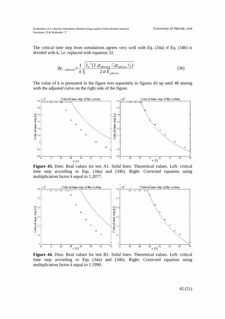
Evaluation of a cohesive interphase element using explicit finite element analysis University of Skövde, 2008 Svensson. D & Walander. T
45 (51)
The critical time step from simulations agrees very well with Eq. (34a) if Eq. (34b) is divided with k, i.e. replaced with equation 32.
adhesive
Hh
adhesiveadherendeadherendc E
L
kt
αρρ
2
)2(1 2 +=∆ (36)
The value of k is presented in the figure text separately in figures 43 up until 48 among with the adjusted curve on the right side of the figure.
Figure 43. Dots: Real values for test A1. Solid lines: Theoretical values. Left: critical time step according to Eqs. (34a) and (34b). Right: Corrected equation using multiplication factor k equal to 1.2077.
Figure 44. Dots: Real values for test B1. Solid lines: Theoretical values. Left: critical time step according to Eqs (34a) and (34b). Right: Corrected equation using multiplication factor k equal to 1.1990.
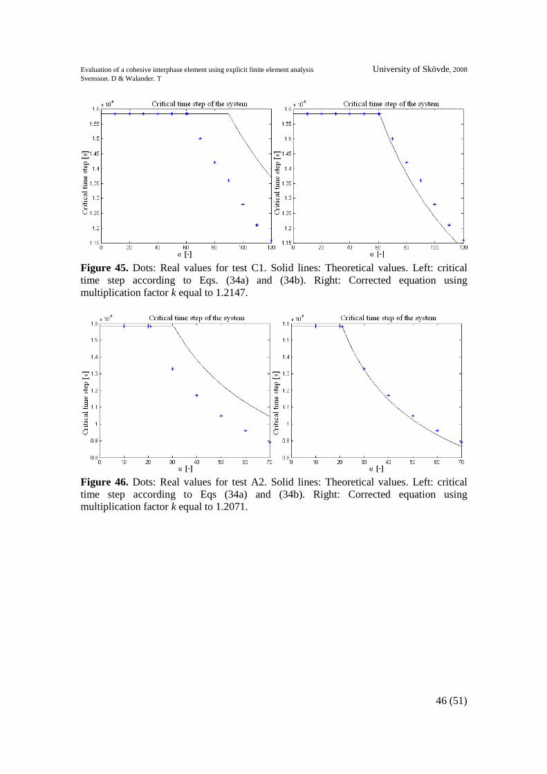
Evaluation of a cohesive interphase element using explicit finite element analysis University of Skövde, 2008 Svensson. D & Walander. T
46 (51)
Figure 45. Dots: Real values for test C1. Solid lines: Theoretical values. Left: critical time step according to Eqs. (34a) and (34b). Right: Corrected equation using multiplication factor k equal to 1.2147.
Figure 46. Dots: Real values for test A2. Solid lines: Theoretical values. Left: critical time step according to Eqs (34a) and (34b). Right: Corrected equation using multiplication factor k equal to 1.2071.
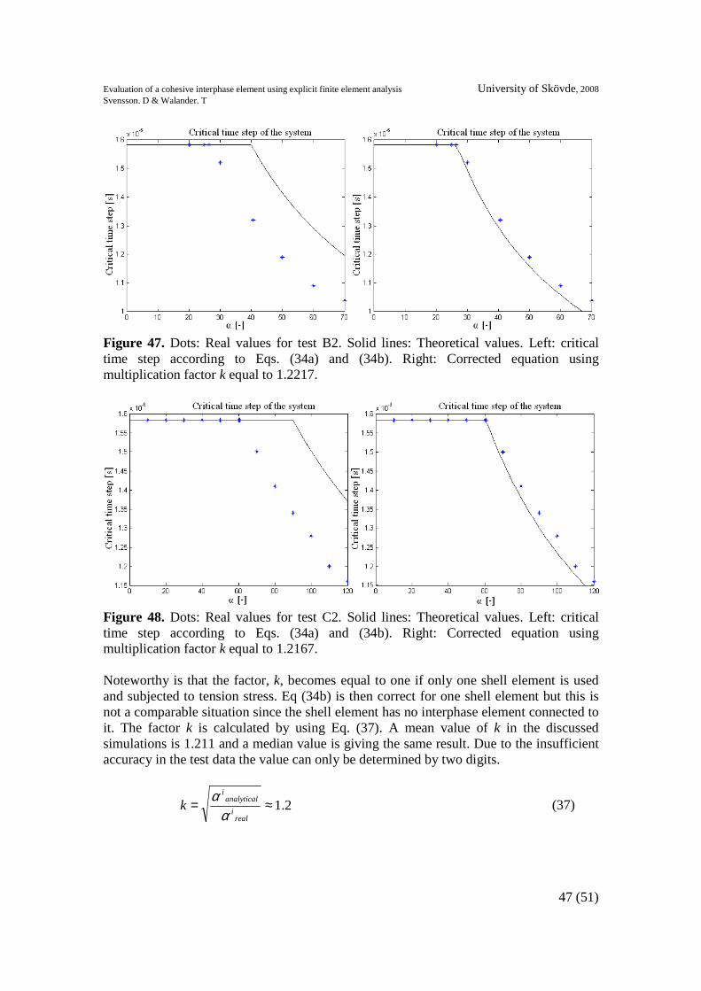
Evaluation of a cohesive interphase element using explicit finite element analysis University of Skövde, 2008 Svensson. D & Walander. T
47 (51)
Figure 47. Dots: Real values for test B2. Solid lines: Theoretical values. Left: critical time step according to Eqs. (34a) and (34b). Right: Corrected equation using multiplication factor k equal to 1.2217.
Figure 48. Dots: Real values for test C2. Solid lines: Theoretical values. Left: critical time step according to Eqs. (34a) and (34b). Right: Corrected equation using multiplication factor k equal to 1.2167. Noteworthy is that the factor, k, becomes equal to one if only one shell element is used and subjected to tension stress. Eq (34b) is then correct for one shell element but this is not a comparable situation since the shell element has no interphase element connected to it. The factor k is calculated by using Eq. (37). A mean value of k in the discussed simulations is 1.211 and a median value is giving the same result. Due to the insufficient accuracy in the test data the value can only be determined by two digits.
2.1≈=real
i
analyticali
kα
α (37)

Evaluation of a cohesive interphase element using explicit finite element analysis University of Skövde, 2008 Svensson. D & Walander. T
48 (51)
The values of the multiplication factor, k, has a small variation and to be conservative the factor 1.25 is recommended to make sure that no analyses will fail due to an invalid time step. Noteworthy is that Abaqus suggests a time step that corresponds to a correction factor of 1.44. By using the Eq. (34) with k equal to 1.25 the runtime can be decreased with 13 percent without losing any accuracy. Simulations have been performed in order to determine if the geometry contributes to the factor k. Two specimens with the same number of nodes and element sizes are studied. What separates the specimens is the length and width. The first specimen has 120 x 4 nodes and the other 160 x 3 and the test is performed in the same manner as the tests described above. That is the value α is varied and the critical time step is investigated. This test indicates that both the tests are getting the same factor since the critical time steps is exactly the same in both cases. Therefore the geometry is not contributing to the factor and thus not affecting the critical time step. The same analyses as with DCB-specimens have also been performed with ENF-specimens. The results of these tests indicate that the critical time steps from simulations for the ENF-specimens correspond exactly with the results for the DCB-simulations. By using Eqs. (34a) and (34b) with the factor k taken in account the critical time step can be predicted for a DCB- or an ENF-simulation regardless of the element mesh. All simulations discussed above are performed with Poisons ratio equal to 0.3 for the adherends. Simulations have been performed with a varying poisons ratio. It is noticed that a smaller value of poisons ratio decreases k, i.e. the critical time step is increased. However this effect is very small. Simulations are performed using a poisons ration equal to zero. The effect of this extreme case is also very small. In other words the failure of Eq. (34b) can not be explained by the influence of Poisons ratio.

Evaluation of a cohesive interphase element using explicit finite element analysis University of Skövde, 2008 Svensson. D & Walander. T
49 (51)
10. Conclusions and future work
10.1 User element All attempts to recreate Tvergaard & Hutchinson-shaped curves for a model consisting of two shell elements and one user elements has been successful. In mixed mode loading the fracture energy is calculated and corresponds well to the pure mode cases. The number of elements in length-row must be equally dividable with the numbers of CPUs that are used in the simulation. This means that the total number of elements must be dividable with the number of processors used in the simulation. A safe way to deal with this is to always have one operating processor but this will increase the runtime quite a lot. The division of processors is always in length-direction independent of node numbers, element numbers and horizontal/vertical direction of long narrow specimen. To enable failure free analyses any operating processor must be fully allocated for only one analysis at the time. To enable more analyzes at the same time the options are: changing the operating computers queue order to only be handling one analysis at the time or halve the numbers of CPUs if possible. No future work is suggested in this subchapter.
10.2 Double Cantilever Beam (DCB) All results obtained from the simulations correspond very well to the theoretical solutions by Tvergaard and Hutchinson cohesive law provided that an appropriate geometry of the specimen is used. If a long initial crack length is used it is necessary to use a specimen that is long enough to make sure the adhesive at the right end is stress free. Furthermore the part of the adherends which are not joined has to be long enough since the equation for energy release rate is based on beam theory. DCB-simulations are performed with distorted element meshes without losing any accuracy in the results. Since all of the DCB-simulations were failure free no future work is recommended.
10.3 End Notch Flexure (ENF) The results from the simulations show a very good agreement with the analytical results when calculating the energy release rate for varying constitutive relations. The agreement indicates that ENF-simulations with the interphase elements give accurate results when analyzing an adhesive layer loaded in shear. However there are some difficulties to capture the correct energy release rate curve from the simulations when using more than four CPUs and a very stiff adhesive layer.
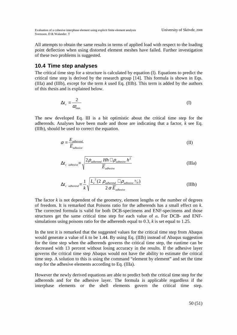
Evaluation of a cohesive interphase element using explicit finite element analysis University of Skövde, 2008 Svensson. D & Walander. T
50 (51)
All attempts to obtain the same results in terms of applied load with respect to the loading point deflection when using distorted element meshes have failed. Further investigation of these two problems is suggested.
10.4 Time step analyses The critical time step for a structure is calculated by equation (I). Equations to predict the critical time step is derived by the research group [14]. This formula is shown in Eqs. (IIIa) and (IIIb), except for the term k used Eq. (IIIb). This term is added by the authors of this thesis and is explained below.
max
2
ω=∆ ct (I)
The new developed Eq. III is a bit optimistic about the critical time step for the adherends. Analyses have been made and those are indicating that a factor, k see Eq. (IIIb), should be used to correct the equation.
adhesive
adherend
E
E=α (II)
adhesive
adhesiveadherendadhesivec E
hHht
22 ρρ +=∆ (IIIa)
adhesive
Hh
adhesiveadherendeadherendc E
L
kt
αρρ
2
)2(1 2 +=∆ (IIIb)
The factor k is not dependent of the geometry, element lengths or the number of degrees of freedom. It is remarked that Poisons ratio for the adherends has a small effect on k. The corrected formula is valid for both DCB-specimens and ENF-specimens and those structures get the same critical time step for each value of α. For DCB- and ENF-simulations using poisons ratio for the adherends equal to 0.3, k is set equal to 1.25. In the test it is remarked that the suggested values for the critical time step from Abaqus would generate a value of k to be 1.44. By using Eq. (IIIb) instead of Abaqus suggestion for the time step when the adherends governs the critical time step, the runtime can be decreased with 13 percent without losing accuracy in the results. If the adhesive layer governs the critical time step Abaqus would not have the ability to estimate the critical time step. A solution to this is using the command “element by element” and set the time step for the adhesive elements according to Eq. (IIIa). However the newly derived equations are able to predict both the critical time step for the adherends and for the adhesive layer. The formula is applicable regardless if the interphase elements or the shell elements govern the critical time step.

Evaluation of a cohesive interphase element using explicit finite element analysis University of Skövde, 2008 Svensson. D & Walander. T
51 (51)
References [1] Wikipedia. Retrieved form internet. http://en.wikipedia.org/wiki/Image:Fracture_modes_v2.svg#file (2008-05-26) [2] Högberg J.L. (2006) Mixed mode cohesive law. Accepted for publication in International Journal of Fracture. [3] Tvergaard V, Hutchinson JW (1992). The relation between crack growth resistance and fracture process parameters in elastic-plastic solids. J Mech Phys Solid 40:1337-1397 [4] Abaqus Analyses Users Manual, v6.6. (2005), Abaqus inc. Avaible on internet: http://abaqus.ethz.ch:2080/v6.6/books/usb/default.htm?startat=pt07ch27s01aus93.html#usb-prc-pamplitude 2008-08-01 [5] Stigh, U. (1988). Damage and crack growth analysis of the double cantilever beam specimen. International Journal of Fracture 37. R13-R18. [6] Andersson, T. (2006). Mechanical behaviour of adhesive layers - methods to extract peel and mixed mode properties. (PhD thesis). Chalmers University of Technology. [7] Salomonsson, K. (2002). Interphase elements connecting structural finite elements - formulation, implementation and verification, M.Sc. Thesis. Chalmers University, Sweden [8] Chai, H. (1988). Shear fracture. International Journal of Fracture 37. 137-157. [9] Alfredsson, K. S. (2004). Constitutive Behaviour and Fracture of Adhesive Layers (PhD thesis). Chalmers Tekniska Högskola, Göteborg. [10] Alfredsson, K. S. (2008). Oral conversations during January 2008 to August 2008. University of Skövde
[11] Salomonsson, K. (2007). Meso-mechanical modeling and analysis of adhesive layers. (PhD thesis). Chalmers University of Technology.
[12] Leffler, K. (2005). Shear Behaviour of Adhesive Layer (Lic.) Chalmers Tekniska Högskola, Göteborg ISSN 1652-8565 2005:15 [13] Carlberger, T. (2006). Impact Simulation of Adhesively Joined Structures. (Lic.). Chalmers Tekniska Högskola, Göteborg. ISSN 1652-8565 2006:11 [14] Stigh, U. 2008. Unpublished material; oral conversations and internal reports during January 2008 to June 2008. Högskolan I Skövde
Related Documents


