Evaluation of a rough soil surface description with ASAR-ENVISAT radar data

www.elsevier.com/locate/rse

Remote Sensing of Environ

Evaluation of a rough soil surface description with

ASAR-ENVISAT radar data

M. Zribia,*, N. Baghdadib, N. Holahb, O. Fafina, C. Guerina

aCETP/CNRS, 10-12 av. de l’Europe, 78140 Velizy, FrancebBureau de Recherches Geologiques et Minieres (BRGM), ARN/ATL 3 av C. Guillemin, B.P. 6009, 45060 Orleans Cedex 2, France

Received 21 July 2004; received in revised form 24 November 2004; accepted 28 November 2004

Abstract

The input roughness parameters for electromagnetic backscattering modelling need to be accurate to estimate radar measurements

correctly over bare soils, particularly in agricultural environments. This paper proposes to evaluate the roughness description in terms of

several characterisations through a correlation function using a numerical backscattering model. The experimental database used in this

study is based on ASAR-ENVISAT experimental campaigns in the Beauce region (France).

Two presentations of the surface height correlation function are proposed in this study. The first one, referred to as the ba functionQ fitsthe experimental correlation functions up to the correlation length, while the second one, the b(a,b) functionQ, fits the correlation function

for scales corresponding to positive values. A relationship is proposed between the rms height of soil surface and the shape of the

correlation function. Using the a function, comparisons between radar measurements for high incidence angles and simulations based on

the numerical backscattering model (moment method) show a good agreement for soil surfaces with an rms height smaller than 2 cm with

medium and high soil moisture.

D 2004 Elsevier Inc. All rights reserved.

Keywords: Radar; ENVISAT; ASAR; Roughness; Backscattering

1. Introduction

Soil moisture and roughness play a key role in hydro-

logical and climate studies. Considerable effort has been

devoted in active microwave remote sensing to study radar

backscattering response from natural surfaces (e.g. Bagh-

dadi et al., 2002, 2004; Jackson et al., 1996; Ulaby et al.,

1986; Zribi & Dechambre, 2002). Electromagnetic back-

scattering models (Kirchoff models, the small perturbation

model (Ulaby et al., 1986)) and more recently, the Integral

Equation Model (IEM, Fung et al., 1992) have been

developed to study this question. However, different

experimental measurements have shown that they were

restricted to smooth or very rough soil surfaces. These

difficulties are attributed to two factors: the first one is the

0034-4257/$ - see front matter D 2004 Elsevier Inc. All rights reserved.

doi:10.1016/j.rse.2004.11.014

* Corresponding author. Tel.: +33 1 39 25 49 34; fax: +33 1 39 25 49

22.

E-mail address: [email protected] (M. Zribi).

soil roughness description based only on two surface

parameters (the rms height (s) and the correlation length

(l)) and generally an exponential correlation function for all

surface types; the second one is the physical approximations

introduced in these models. For example, the small

perturbation model (SPM) is valid only for very smooth

soils, Kirchoff approximations correspond to very rough

surfaces, and for IEM, it is still difficult to identify a large

validity domain for real agricultural soils in spite of the

improvements developed over the past few years (Chen et

al., 2000; Wu et al., 2001).

The developed backscattering models generally neglect

the volumetric contribution of soil. This hypothesis limits

their validation to low surface moisture, where wave

penetration is large (Fung, 1994).

In that context, over the last few years, different studies

have tried to introduce a more complete description of soil

surface roughness for forward studies (Davidson et al., 2000;

Li et al., 2002; Mattia & Le Toan, 1999; Mattia et al., 2003;

ment 95 (2005) 67–76

M. Zribi et al. / Remote Sensing of Environment 95 (2005) 67–7668

Oh & Kay, 1998; Zribi et al., 2000). The classical one, which

is based just on s and l with a fixed correlation function

neglects the importance of the shape of the correlation

function and its strong effect on backscattering. Recent

approaches generally show that a single-scale description of

the soil surface is not sufficient to describe all the scales of

soil roughness. Zribi et al. (2000) proposed a fractal brownian

model to introduce the description of soil roughness for an

interval of scales. This approach adds the fractal dimension

for scale characterisation. It links the shape of the correlation

function to the fractal dimension. Mattia and Le Toan (1999)

proposed a multi-scale gaussian description. These fractal

and multi-scale approaches do not consider stationary

profiles. Li et al. (2002) propose a generalized power-law

spectral density with a new parameterisation for a surface

considered as stationary. This results in a precise spectrum

evolution between exponential and gaussian surfaces. The

complexity of these approaches exists particularly in the

estimation of the proposed parameters from real experimental

profiles. These studies, based generally on a complex

parameterisation of surface roughness, have introduced

great improvements in the radar signal simulations for a

large domain of surface roughness. However, if we try to

analyse the inversion of radar signals, a simple description of

surface roughness is still needed because of difficulties

when complex parameterisations of heights are used.

In this paper, we investigate the characterisation of

roughness in terms of several simplified descriptions of the

correlation function using a numerical backscattering model.

Two types of correlation functions are proposed. These

descriptions are validated with ASAR-ENVISAT data for

different experimental campaigns in France. An exact

backscattering numerical model based on the moment

method (MM) is used to evaluate the discussed roughness

description.

In Section 2, we present the experimental data set, built

with both ground truth measurements (roughness and soil

moisture) and ASAR-ENVISAT data. In Section 3, we

present the surface roughness characterisation based on

different descriptions of the correlation function of surface

heights. The backscattering numerical simulation approach

based on the moment method (MM) applied with these

roughness descriptions is briefly presented. Section 4

discusses the results obtained by comparing ASAR-ENVI-

SAT measurements with MM simulations using the pro-

posed roughness description. Conclusions are gathered in

Section 5.

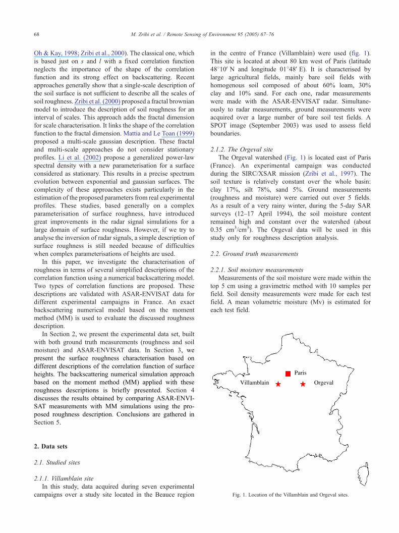
Fig. 1. Location of the Villamblain and Orgeval sites.

2. Data sets

2.1. Studied sites

2.1.1. Villamblain site

In this study, data acquired during seven experimental

campaigns over a study site located in the Beauce region

in the centre of France (Villamblain) were used (fig. 1).

This site is located at about 80 km west of Paris (latitude

48810VN and longitude 01848VE). It is characterised by

large agricultural fields, mainly bare soil fields with

homogenous soil composed of about 60% loam, 30%

clay and 10% sand. For each one, radar measurements

were made with the ASAR-ENVISAT radar. Simultane-

ously to radar measurements, ground measurements were

acquired over a large number of bare soil test fields. A

SPOT image (September 2003) was used to assess field

boundaries.

2.1.2. The Orgeval site

The Orgeval watershed (Fig. 1) is located east of Paris

(France). An experimental campaign was conducted

during the SIRC/XSAR mission (Zribi et al., 1997). The

soil texture is relatively constant over the whole basin:

clay 17%, silt 78%, sand 5%. Ground measurements

(roughness and moisture) were carried out over 5 fields.

As a result of a very rainy winter, during the 5-day SAR

surveys (12–17 April 1994), the soil moisture content

remained high and constant over the watershed (about

0.35 cm3/cm3). The Orgeval data will be used in this

study only for roughness description analysis.

2.2. Ground truth measurements

2.2.1. Soil moisture measurements

Measurements of the soil moisture were made within the

top 5 cm using a gravimetric method with 10 samples per

field. Soil density measurements were made for each test

field. A mean volumetric moisture (Mv) is estimated for

each test field.

1 Km

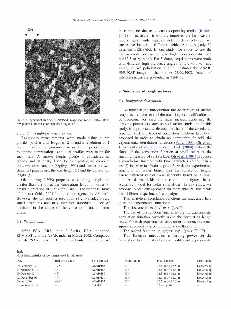
Fig. 2. A segment of an ASAR ENVISAT image acquired in 23/09/2003 in

HH polarisation and at an incidence angle of 408.

M. Zribi et al. / Remote Sensing of Environment 95 (2005) 67–76 69

2.2.2. Soil roughness measurements

Roughness measurements were made using a pin

profiler (with a total length of 2 m and a resolution of 1

cm). In order to guarantee a sufficient precision in

roughness computations, about 10 profiles were taken for

each field. A surface height profile is considered as

ergodic and stationary. Then, for each profile, we compute

the correlation function (Ogilvy, 1991) and derive the two

statistical parameters, the rms height (s) and the correlation

length (l).

Oh and Kay (1998) proposed a sampling length not

greater than 0.2 times the correlation length in order to

obtain a precision of F5% for s and l. For our case, most

of the test fields fulfil this condition (generally lN5 cm).

However, the pin profiler resolution (1 cm) neglects very

small structures and may therefore introduce a lack of

precision in the shape of the correlation function near

origin.

2.3. Satellite data

After ESA, ERS1 and 2 SARs, ESA launched

ENVISAT with the ASAR radar in March 2002. Compared

to ERS/SAR, this instrument extends the range of

Table 1

Main characteristics of the images used in this study

Date Incidence angle Sensor/mode

09 February 03 37.58 ASAR/IS5

23 September 03 408 ASAR/IS6

09 October 03 438 ASAR/IS7

02 December 03 408 ASAR/IS6

06 mai 2004 44.48 ASAR/IS7

04 September 03 – SPOT4

measurements due to its various operating modes (Rosich,

2002). In particular, it strongly improves on the measure-

ments repeat with approximately 5 days between two

successive images at different incidence angles (only 35

days for ERS/SAR). In our study, we chose to use the

narrow mode corresponding to high resolution data (12.5

m�12.5 m by pixel). For 5 dates, acquisitions were made

with different high incidence angles (37.58, 408, 438 and

44.58) in HH polarisation. Fig. 2 illustrates the ASAR-

ENVISAT image of the site on 23/09/2003. Details of

satellite images are presented in Table 1.

3. Simulation of rough surfaces

3.1. Roughness description

As noted in the Introduction, the description of surface

roughness remains one of the most important difficulties to

be overcome for inverting radar measurements and the

deriving parameters such as soil surface moisture. In this

study, it is proposed to discuss the shape of the correlation

function. Different types of correlation functions have been

proposed in order to obtain an appropriate fit with the

experimental correlation functions (Fung, 1994; Oh et al.,

1994; Zribi et al., 2000). Zribi et al. (2000) linked the

shape of the correlation function at small scales to the

fractal dimension of soil surface. Oh et al. (1994) proposed

a correlation function with two parameters (other than s

and l) in order to obtain a good fit with the experimental

functions for scales larger than the correlation length.

These different studies were generally based on a small

number of test fields and also on an analytical back-

scattering model for radar simulations. In this study, we

propose to test our approach on more than 50 test fields

and different experimental campaigns.

Two analytical correlation functions are suggested here

to fit the experimental functions:

The first one is: q(x)=s2 exp�((x/l)a)

The use of this function aims at fitting the experimental

correlation function correctly up to the correlation length

scale. For each experimental correlation function, the mean

square approach is used to compute coefficient a.The second function is: q(x)=s2 exp�

�(x/l)[a+b(x/l)]

�

This function introduces a varying power for the

correlation function. As observed in different experimental

Polarisation Pixel spacing Orbit mode

HH 12.5 m by 12.5 m Descending

HH 12.5 m by 12.5 m Descending

HH 12.5 m by 12.5 m Descending

HH 12.5 m by 12.5 m Descending

HH 12.5 m by 12.5 m Descending

– 20 m by 20 m –

0

0,1

0,2

0,3

0,4

0,5

0,6

0,7

0,8

0,9

1

0 5 10 15 20

Nor

mal

ized

cor

rela

tion

experimental correlation function

Gaussian function

alpha function

a, b, function

exponential function

0

0,1

0,2

0,3

0,4

0,5

0,6

0,7

0,8

0,9

1

0 5 10 15 20

Displacement (cm)

Displacement (cm)

Nom

aliz

ed c

orre

latio

n

experimental correlation function

Gaussian function

alpha function

a, b, function

exponential function

(a)

(b)

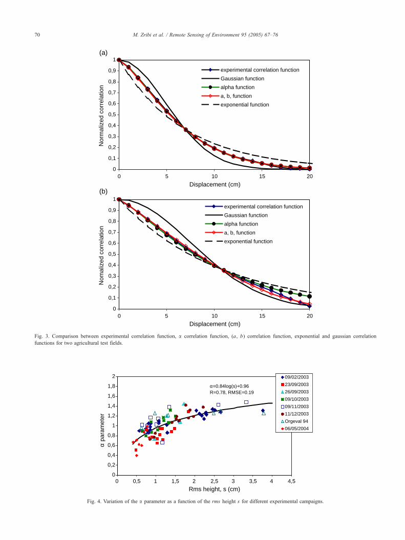
Fig. 3. Comparison between experimental correlation function, a correlation function, (a, b) correlation function, exponential and gaussian correlation

functions for two agricultural test fields.

0

0,2

0,4

0,6

0,8

1

1,2

1,4

1,6

1,8

2

0 1 2 3 40,5 1,5 2,5 3,5 4,5

Rms height, s (cm)

α pa

ram

eter

09/02/2003

23/09/2003

26/09/2003

09/10/2003

09/11/2003

11/12/2003

Orgeval 94

06/05/2004

α=0.84log(s)+0.96 R=0.78, RMSE=0.19

Fig. 4. Variation of the a parameter as a function of the rms height s for different experimental campaigns.

M. Zribi et al. / Remote Sensing of Environment 95 (2005) 67–7670

M. Zribi et al. / Remote Sensing of Environment 95 (2005) 67–76 71

profiles, the shape of the correlation function is not usually

stable with a constant power, particularly beyond the

correlation length scale. Coefficients a and b are computed

by a mean square approach for positive correlation function

values. When b is close to zero, this means that the

correlation function could be simply fitted by a function

with a constant power. On the other hand, when b is large,

the shape of the function beyond the correlation length scale

corresponds more to a gaussian correlation function. This

case is largely present in real agricultural surfaces, as will be

illustrated below.

As an example, Fig. 3 shows a comparison of two

experimental correlation functions and the two proposed

correlation functions, where the gaussian and exponential

0

0,2

0,4

0,6

0,8

1

1,2

1,4

1,6

1,8

2

0 0,2 0,4 0,6 0,8

a par

α pa

ram

eter

(a)

(b)

-0,2

0

0,2

0,4

0,6

0,8

1

0 0,5 1 1,5

Rms he

b pa

ram

eter

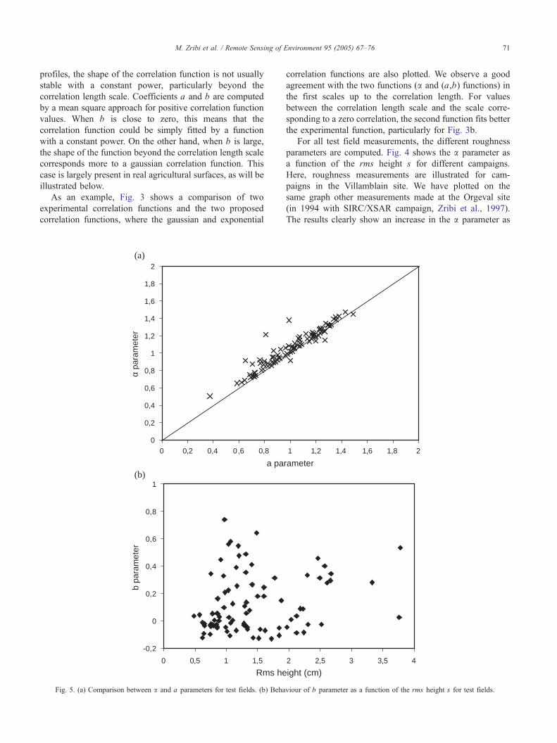
Fig. 5. (a) Comparison between a and a parameters for test fields. (b) Beha

correlation functions are also plotted. We observe a good

agreement with the two functions (a and (a,b) functions) in

the first scales up to the correlation length. For values

between the correlation length scale and the scale corre-

sponding to a zero correlation, the second function fits better

the experimental function, particularly for Fig. 3b.

For all test field measurements, the different roughness

parameters are computed. Fig. 4 shows the a parameter as

a function of the rms height s for different campaigns.

Here, roughness measurements are illustrated for cam-

paigns in the Villamblain site. We have plotted on the

same graph other measurements made at the Orgeval site

(in 1994 with SIRC/XSAR campaign, Zribi et al., 1997).

The results clearly show an increase in the a parameter as

1 1,2 1,4 1,6 1,8 2

ameter

2 2,5 3 3,5 4

ight (cm)

viour of b parameter as a function of the rms height s for test fields.

M. Zribi et al. / Remote Sensing of Environment 95 (2005) 67–7672

a function of the rms height before an approximate settling

at high roughness values. This could be explained by the

fact that for small roughness values we have generally

more small clods and therefore a larger power at high

frequencies, and therefore a smaller a. High rms height

corresponds generally to ploughed soils with principally

large clods and then a limited power at high frequencies.

The second important observation deals with the

behaviour of a for the different campaigns. The a values

have a general tendency to increase with the oldness of the

agricultural tillage and soil moisture, except for rough

surfaces (sN1.5 cm). This behaviour is due particularly to

the effect of rain on the degradation of small clods (high-

frequency structures) and then the increase in a. For

surfaces with large rms height, the limited high-frequency

power explains the absence of tendency for a.In fact, the smallest values are generally retrieved

approximately for the dates 23/09/2003 and 26/09/2003.

These dates correspond to new agricultural tillage and

small or medium values of soil moisture (mean Mv equals

to 7 and 18%). For 09/10/2003 and 03/11/2003 measure-

ments, with rainfall after the end of September measure-

ments, soil has been degraded which induced an increase

in the a parameter. The date 11/12/2003 corresponds to

new tillage made at the beginning of December but

followed by large rainfall (mean Mv of about 30%).

During the Orgeval campaign, the highest a values are

observed. The measurements were made in April 1994

after a long period without agricultural tillage and strong

rainfall (mean soil moisture of about 35%). The date of 06/

05/2004 corresponds to the case of very smooth soil

surfaces with small a parameters.

To conclude on these results, it may be observed that

the a parameter might be one of the tools for quantifying

the evolution of soil surface structure and degradation, an

important parameter for agronomic and erosion studies

(Boiffin & Monnier, 1985; Le Bissonnais et al., 1989).

An empirical logarithmic relationship is proposed to link

the rms height to the a parameter with a high correlation

-20

0

20

40

60

80

100

120

0 200 400Distanc

Hei

ght (

mm

)

Fig. 6. Generation of three surfaces with s=0,7 cm

coefficient (R=0.78) and a root mean square error equal to

0.19. It is written as:

a ¼ 0:84log sð Þ þ 0:96 ð1Þ

This relationship could be considered as a tool for

eliminating one parameter (the shape of the correlation

function) in the inversion of radar measurements.

The a and b parameters of the second proposed function

are also computed over the whole set of measured soil

profiles. As observed in Fig. 5a, a and a are generally close,

particularly for surfaces with very small b values. On the

other hand, the second parameter b is not very stable. This is

illustrated in Fig. 5b, where b is plotted as function of the

rms height. We do not observe any significant correlation

between the rms height and the b parameter.

3.2. Simulation of soil surfaces

In order to study the backscattering behaviour of soil

surfaces and to estimate the difference between the two

proposed functions, we chose to use a numerical model

based on the moment method. This numerical approach

needs a generation of soil surface as input to roughness

description.

For the simulation of surface, we used the approach

described by Fung and Chen (1985), as follows:

The surface heights are written as:

h kð Þ ¼Xi¼M

i¼�M

W ið ÞX iþ kð Þ ð2Þ

where X(i) is a gaussian random variable N(0,1) and W( j) is

the weighting function given by W ið Þ ¼ F�1tffiffiffiffiffiffiffiffiffiffiffiffiffiffiffiF C ið Þ½ �

pb,

where C(i) is the correlation function and F[] denotes the

Fourier transform operator.

For the proposed functions, there is no obvious analytical

Fourier transformation of the correlation functions. There-

fore, Fast Fourier Transformation (FFT) is used to compute

the corresponding values numerically.

600 800 1000e (mm)

s=7mm, l=60 mm

α =1.6

α =1.3

α =1

, l=6 cm and (a) a=1, (b) a=1.3, (c) a=1.6.

-12

-10

-8

-6

-4

-2

0

2

-12 -10 -8 -6 -4 -2 0 2

Simulations (α function)

Sim

ulat

ions

((a

, b)

func

tion)

incidence=26˚incidence=42˚

RMSE=0.18dB (26˚)

RMSE=0.36dB (42˚)

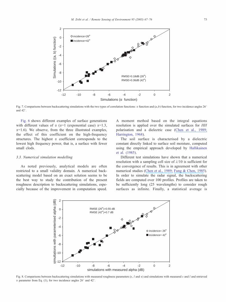
Fig. 7. Comparisons between backscattering simulations with the two types of correlation functions: a function and (a,b) function, for two incidence angles 268and 428.

M. Zribi et al. / Remote Sensing of Environment 95 (2005) 67–76 73

Fig. 6 shows different examples of surface generations

with different values of a (a=1 (exponential case) a=1.3,a=1.6). We observe, from the three illustrated examples,

the effect of this coefficient on the high-frequency

structures. The highest a coefficient corresponds to the

lowest high frequency power, that is, a surface with fewer

small clods.

3.3. Numerical simulation modelling

As noted previously, analytical models are often

restricted to a small validity domain. A numerical back-

scattering model based on an exact solution seems to be

the best way to study the contribution of the present

roughness description to backscattering simulations, espe-

cially because of the improvement in computation speed.

-12

-10

-8

-6

-4

-2

0

2

-12 -10 -8 -6simulations with m

sim

ulta

tions

with

par

amet

eris

ed a

lpha

(dB

)

RMSE (26˚)=0.55 dBRMSE (42˚)=0.7 dB

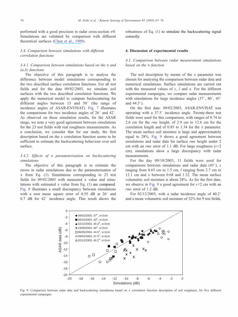
Fig. 8. Comparisons between backscattering simulations with measured roughness

a parameter from Eq. (1), for two incidence angles 268 and 428.

A moment method based on the integral equations

resolution is applied over the simulated surfaces for HH

polarisation and a dielectric case (Chen et al., 1989;

Harrington, 1968).

The soil surface is characterised by a dielectric

constant directly linked to surface soil moisture, computed

using the empirical approach developed by Hallikainen

et al. (1985).

Different test simulations have shown that a numerical

resolution with a sampling cell size of k/10 is sufficient for

the convergence of results. This is in agreement with other

numerical studies (Chen et al., 1989; Fung & Chen, 1985).

In order to simulate the radar signal, the backscattering

fields are computed over 100 profiles. Profiles are taken to

be sufficiently long (25 wavelengths) to consider rough

surfaces as infinite. Finally, a statistical average is

-4 -2 0 2easured alpha (dB)

incidence= 26˚incidence= 42˚

parameters (s, l and a) and simulations with measured s and l and retrieved

M. Zribi et al. / Remote Sensing of Environment 95 (2005) 67–7674

performed with a good precision in radar cross-section r0.Simulations are validated by comparison with different

theoretical surfaces (Chen et al., 1989).

3.4. Comparison between simulations with different

correlation functions

3.4.1. Comparison between simulations based on the a and

(a,b) functions

The objective of this paragraph is to analyse the

difference between model simulations corresponding to

the two described surface correlation functions. For all test

fields and for the date 09/02/2003, we simulate soil

surfaces with the two described correlation functions. We

apply the numerical model to compute backscattering for

different angles between 15 and 508 (the range of

incidence angles of ASAR-ENVISAT). Fig. 7 illustrates

the comparisons for two incidence angles of 268 and 428.As observed on these simulation results, for the ASAR

range, we note a very good agreement between simulations

for the 23 test fields with real roughness measurements. As

a conclusion, we consider that for our study, the first

description based on the a correlation function seems to be

sufficient to estimate the backscattering behaviour over soil

surface.

3.4.2. Effects of a parameterisation on backscattering

simulations

The objective of this paragraph is to estimate the

errors in radar simulations due to the parameterisation of

a from Eq. (1). Simulations corresponding to 23 test

fields for 09/02/2003 with measured a value and simu-

lations with estimated a value from Eq. (1) are compared.

Fig. 8 illustrates a small discrepancy between simulations

with a root mean square error of 0.55 dB at 268 and

0.7 dB for 428 incidence angle. This result shows the

-20

-18

-16

-14

-12

-10

-8

-6

-4

-2

0

-20 -18 -16 -14 -12 -

Simulat

AS

AR

dat

a (d

B)

09/02/2003, 37˚, s<2cm

09/10/2003, 43˚, s<2cm

02/12/2003, 40.2˚, s<2cm

23/09/2004, 40˚, s<2cm

06/05/2004, 44.5˚, s<2cm

09/02/2003, 37.5˚, s>2cm

02/12/2003, 40.2˚, s>2cm

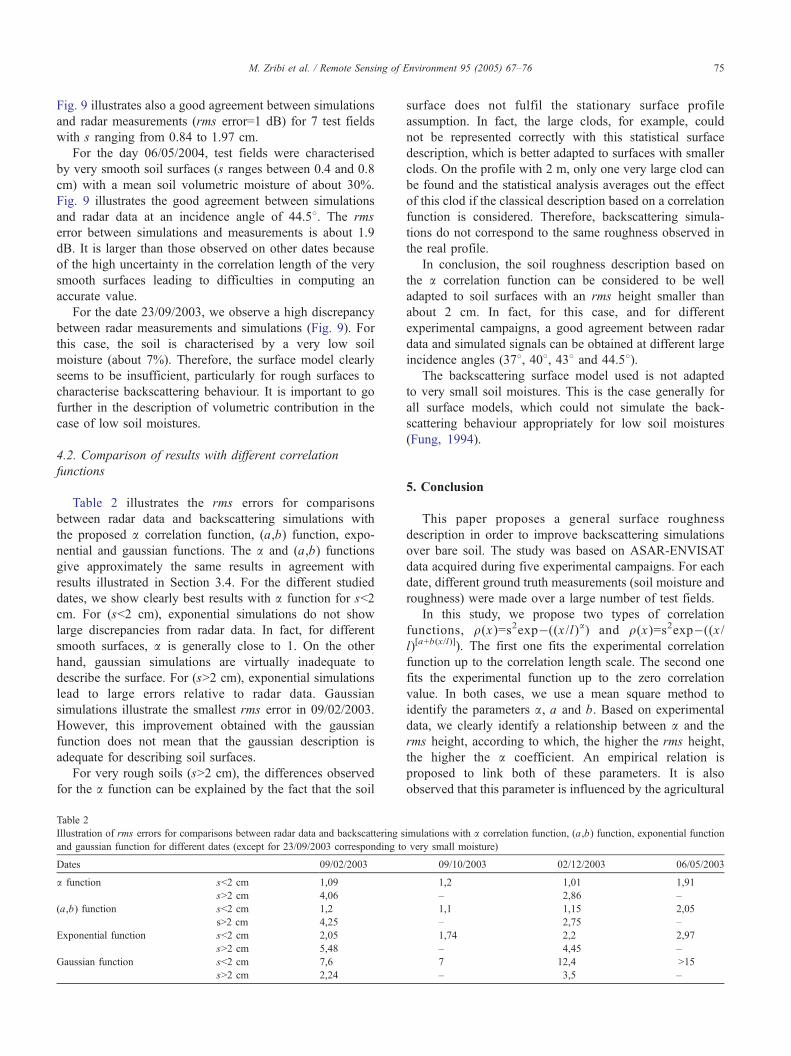
Fig. 9. Comparison between radar data and backscattering simulations based o

experimental campaigns.

robustness of Eq. (1) to simulate the backscattering signal

correctly.

4. Discussion of experimental results

4.1. Comparison between radar measurement simulations

based on the a function

The soil description by means of the a parameter was

chosen for analysing the comparison between radar data and

numerical simulations. Surface simulations are carried out

with the measured values of s, l and a. For the different

experimental campaigns, we compare radar measurements

with simulations for large incidence angles (378, 408, 438and 44.58).

On the first date: 09/02/2003, ASAR-ENVISAT was

operating with a 37.58 incidence angle. Twenty-three test

fields were used for this comparison, with ranges of 0.74 to

2.6 cm for the rms height, of 2.9 cm to 12.6 cm for the

correlation length and of 0.85 to 1.34 for the a parameter.

The mean surface soil moisture is large and approximately

equal to 28%. Fig. 9 shows a good agreement between

simulations and radar data for surface rms height under 2

cm with an rms error of 1.1 dB. For large roughness (sN2

cm), simulations show a large discrepancy with radar

measurements.

For the day 09/10/2003, 11 fields were used for

comparisons between simulations and radar data (438), sranging from 0.65 cm to 1.5 cm, l ranging from 2.7 cm to

12.1 cm and a between 0.68 and 1.32. The mean surface

volumetric soil moisture is about 24%. As for the first date,

we observe in Fig. 9 a good agreement for sb2 cm with an

rms error of 1.2 dB.

For 02/12/2003, with a radar incidence angle of 40.28and a mean volumetric soil moisture of 32% for 9 test fields,

10 -8 -6 -4 -2 0

ions (dB)

n a correlation function description of soil roughness, for five different

M. Zribi et al. / Remote Sensing of Environment 95 (2005) 67–76 75

Fig. 9 illustrates also a good agreement between simulations

and radar measurements (rms error=1 dB) for 7 test fields

with s ranging from 0.84 to 1.97 cm.

For the day 06/05/2004, test fields were characterised

by very smooth soil surfaces (s ranges between 0.4 and 0.8

cm) with a mean soil volumetric moisture of about 30%.

Fig. 9 illustrates the good agreement between simulations

and radar data at an incidence angle of 44.58. The rms

error between simulations and measurements is about 1.9

dB. It is larger than those observed on other dates because

of the high uncertainty in the correlation length of the very

smooth surfaces leading to difficulties in computing an

accurate value.

For the date 23/09/2003, we observe a high discrepancy

between radar measurements and simulations (Fig. 9). For

this case, the soil is characterised by a very low soil

moisture (about 7%). Therefore, the surface model clearly

seems to be insufficient, particularly for rough surfaces to

characterise backscattering behaviour. It is important to go

further in the description of volumetric contribution in the

case of low soil moistures.

4.2. Comparison of results with different correlation

functions

Table 2 illustrates the rms errors for comparisons

between radar data and backscattering simulations with

the proposed a correlation function, (a,b) function, expo-

nential and gaussian functions. The a and (a,b) functions

give approximately the same results in agreement with

results illustrated in Section 3.4. For the different studied

dates, we show clearly best results with a function for sb2

cm. For (sb2 cm), exponential simulations do not show

large discrepancies from radar data. In fact, for different

smooth surfaces, a is generally close to 1. On the other

hand, gaussian simulations are virtually inadequate to

describe the surface. For (sN2 cm), exponential simulations

lead to large errors relative to radar data. Gaussian

simulations illustrate the smallest rms error in 09/02/2003.

However, this improvement obtained with the gaussian

function does not mean that the gaussian description is

adequate for describing soil surfaces.

For very rough soils (sN2 cm), the differences observed

for the a function can be explained by the fact that the soil

Table 2

Illustration of rms errors for comparisons between radar data and backscattering s

and gaussian function for different dates (except for 23/09/2003 corresponding to

Dates 09/02/2003

a function sb2 cm 1,09

sN2 cm 4,06

(a,b) function sb2 cm 1,2

sN2 cm 4,25

Exponential function sb2 cm 2,05

sN2 cm 5,48

Gaussian function sb2 cm 7,6

sN2 cm 2,24

surface does not fulfil the stationary surface profile

assumption. In fact, the large clods, for example, could

not be represented correctly with this statistical surface

description, which is better adapted to surfaces with smaller

clods. On the profile with 2 m, only one very large clod can

be found and the statistical analysis averages out the effect

of this clod if the classical description based on a correlation

function is considered. Therefore, backscattering simula-

tions do not correspond to the same roughness observed in

the real profile.

In conclusion, the soil roughness description based on

the a correlation function can be considered to be well

adapted to soil surfaces with an rms height smaller than

about 2 cm. In fact, for this case, and for different

experimental campaigns, a good agreement between radar

data and simulated signals can be obtained at different large

incidence angles (378, 408, 438 and 44.58).The backscattering surface model used is not adapted

to very small soil moistures. This is the case generally for

all surface models, which could not simulate the back-

scattering behaviour appropriately for low soil moistures

(Fung, 1994).

5. Conclusion

This paper proposes a general surface roughness

description in order to improve backscattering simulations

over bare soil. The study was based on ASAR-ENVISAT

data acquired during five experimental campaigns. For each

date, different ground truth measurements (soil moisture and

roughness) were made over a large number of test fields.

In this study, we propose two types of correlation

functions, q(x )=s2exp�((x /l)a) and q(x )=s2exp�((x /

l)[a+b(x/l)]). The first one fits the experimental correlation

function up to the correlation length scale. The second one

fits the experimental function up to the zero correlation

value. In both cases, we use a mean square method to

identify the parameters a, a and b. Based on experimental

data, we clearly identify a relationship between a and the

rms height, according to which, the higher the rms height,

the higher the a coefficient. An empirical relation is

proposed to link both of these parameters. It is also

observed that this parameter is influenced by the agricultural

imulations with a correlation function, (a,b) function, exponential function

very small moisture)

09/10/2003 02/12/2003 06/05/2003

1,2 1,01 1,91

– 2,86 –

1,1 1,15 2,05

– 2,75 –

1,74 2,2 2,97

– 4,45 –

7 12,4 N15

– 3,5 –

M. Zribi et al. / Remote Sensing of Environment 95 (2005) 67–7676

soil tillage evolution and rainfall. It will be important to link

it in more detail with soil structure, an important input

parameter for erosion and agronomical studies.

The numerical model based on the moment method is

used to assess the contribution of these functions. It is

shown that for the range of incidence angles of ASAR-

ENVISAT (158, 478), there is very little difference between

both cases and therefore, the function with a fixed power

seems to be sufficient.

The comparison between radar measurements and

simulations shows that for high and medium soil moistures,

a good agreement exists between data and model simu-

lations for soil rms heights below 2 cm. For higher rms

heights, a discrepancy exists with simulations. This is

probably due to the complexity of the soil surface and the

fact that the approach assuming a stationary profile and

based on a correlation function is not appropriate.

In the next studies, it will be important to further describe

very rough surfaces with other methodologies, particularly

to better take into account the distribution of clod sizes.

The proposed approach describing the isotropic structure

of soil surface is applied to large incidence angles in C band.

For other conditions of frequency or incidence angle, this

description could become part of a more complete descrip-

tion (for example, adding information from larger scales

such as rows).

Acknowledgements

This work was financed by two programs PNTS

(French Program of Remote Sensing) and PNRH (French

Program of Hydrological, project RIDES). The authors

would like to thank the European Space Agency (ESA) for

providing us with the ASAR images free of charge through

the project n8351 ENVISAT/ASAR. The SPOT images

were obtained through the CNES’ ISIS program (Centre

National d’Etudes Spatiales). The authors would also like

to thank Monique Dechambre, Isabella Zin, Catherine

Ottle, Steven Hosford, Odile Duval and Olivier Cerdan

and the whole team for their logistic support in terrain

campaigns.

References

Baghdadi, N., Gaultier, S., & King, C. (2002). Retrieving surface roughness

and soil moisture from SAR data using neural network. Canadian

Journal of Remote Sensing, 28(5), 701–711.

Baghdadi, N., Gherboudj, I., Zribi, M., Sahebi, M., Bonn, F., & King,

C. (2004). Semi-empirical calibration of the IEM backscattering

model using radar images and moisture and roughness field

measurements. International Journal of Remote Sensing, 25(18),

3593–3623.

Boiffin, J., & Monnier, G. (1985). Infiltration rate as influenced by soil

surface crusting caused by rainfall. In F. Callebaut, D. Gabriels, & M.

De Boodt (Eds.), Assessment of soil surface sealing and crusting,

Proceeding of Symposium helt in Gent, Belguim (pp. 210–217).

Chen, K. -S., Wu, T. D., Tsay, M. K., & Fung, A. K. (2000). A note on the

multiple scattering in an IEM model. IEEE Transactions on Geoscience

and Remote Sensing, 38(1), 249–256.

Chen, M. F., Chen, K. S., & Fung, A. K. (1989). A study of the validity of

the Integral Equation Model by moment method simulation-cylindrical

case. Remote Sensing of Environment, 29, 217–228.

Davidson, M. W. J., Le Toan, T., Mattia, F., Satalino, G., Manninen, T., &

Borgeaud, M. (2000). On the characterisation of agricultural soil

roughness for radar remote sensing studies. IEEE Transactions on

Geoscience and Remote Sensing, 38, 630–640.

Fung, A., & Chen, M.F. (1985). Numerical simulation of scattering from

simple and composite random surfaces. Journal of the Optical Society

America. A, 2(12), 2274–2283.

Fung, A. K. (1994). Microwave scattering and emission models and their

applications. Artech House.

Fung, A. K., Li, Z., & Chen, K. S. (1992). Backscattering from a randomly

rough dielectric surface. IEEE Transactions on Geoscience and Remote

Sensing, 30(2), 356–369.

Hallikainen, M. T., Ulaby, F. T., Dobson, M. C., El-Rayes, M. A., & Wu, L.

K. (1985). Microwave dielectric behaviour of wet soil: Part I. Empirical

models and experimental observations. IEEE Transactions on Geo-

science and Remote Sensing, 23(1), 25–46.

Harrington, R. F. (1968). Field computation by moment method. Series on

electromagnetic waves. IEEE PRESS.

Jackson, T. -J., Schmugge, J., & Engman, E. -T. (1996). Remote sensing

applications to hydrology: Soil moisture. Hydrological Sciences, 41(4),

517–530.

Le Bissonnais, Y., Bruand, A., & Jamagne, M. (1989). Laboratory

experimental study of soil crusting: Relation between aggregates

breakdown and crust structure. Catena, 16, 377–392.

Li, Q., Shi, J.C., & Chen, K.-S. (2002). A generalized power law spectrum

and its applications to the backscattering of soil surfaces based on the

integral equation model. IEEE Transactions on Geoscience and Remote

Sensing, 40(2), 271–281.

Mattia, F., Davidson, W. J., Le Toan, T., D’Haese, M. F., Verhost, N. E. C.,

Gatti, A. M., et al. (2003). A comparison between soil roughness

statistics used in surface scattering models derived from mechanical and

laser profilers. IEEE Transactions on Geoscience and Remote Sensing,

41(7), 1659–1671.

Mattia, F., & Le Toan, T. (1999). Backscattering properties of multi-scale

rough surfaces. Journal of Electromagnetic Waves and Applications, 13,

491–526.

Ogilvy, O. (1991). Theory of wave scattering from random rough surfaces.

Adam Hilder.

Oh, Y., & Kay, Y. C. (1998). Condition for precise measurement of soil

surface roughness. IEEE Transactions on Geoscience and Remote

Sensing, 36(2), 691–695.

Oh, Y., Sarabandi, K., & Ulaby, F. T. (1994). An inversion algorithm to

retrieve soil moisture and surface roughness from polarimetric radar

observations. Proc of IGARSS’94, Firenze, Italy.

Rosich, (2002). ASAR validation review, ESRIN, Frescatti, 11–12

December, 2002.

Ulaby, F. T., Moore, R. K., & Fung, A. K. (1986). Microwave remote

sensing active and passive. Artech House.

Wu, T. D., Chen, K. S., Shi, J., & Fung, A. K. (2001). A transition model

for the reflection coefficient in surface scattering. IEEE Transactions on

Geoscience and Remote Sensing, 39(9), 2040–2050.

Zribi, M., & Ciarletti, V. (2000). Validation of a rough surface model based

on fractional brownian geometry with SIRC and ERASME radar data

over Orgeval site. Remote Sensing of Environment, 73, 65–72.

Zribi, M., & Dechambre, M. (2002). An new empirical model to retrieve

soil moisture and roughness from radar data. Remote Sensing of

Environment, 84(1), 42–52.

Zribi, M., Taconet, O., Le Hegarat-Mascle, S., Vidal-Madjar, D., Emblanch,

C., Loumagne, C., et al. (1997). Backscattering behavior and simulation

comparison over bare soils using SIRC/XSAR and ERASME 1994 data

over Orgeval. Remote Sensing of Environment, 59, 256–266.