June 2009 Ole Jørgen Nydal, EPT Kjartan Berg, Kongsberg Maritime Stein Tore Johansen, SINTEF Master of Science in Energy and Environment Submission date: Supervisor: Co-supervisor: Norwegian University of Science and Technology Department of Energy and Process Engineering Evaluation of a Flow Simulator for Multiphase Pipelines Jeppe Mathias Jansen

Welcome message from author
This document is posted to help you gain knowledge. Please leave a comment to let me know what you think about it! Share it to your friends and learn new things together.
Transcript

June 2009Ole Jørgen Nydal, EPTKjartan Berg, Kongsberg MaritimeStein Tore Johansen, SINTEF
Master of Science in Energy and EnvironmentSubmission date:Supervisor:Co-supervisor:
Norwegian University of Science and TechnologyDepartment of Energy and Process Engineering
Evaluation of a Flow Simulator forMultiphase Pipelines
Jeppe Mathias Jansen


Problem DescriptionBackgroundMultiphase flow simulators are used for flow assurance analysis, design and support for oil andgas transportation processes in pipelines and in process equipment. Keywords for the futurechallenges are deep water, long distances, complex geometry and complex fluids. Newdevelopment tools are being developed for simulations of multiphase pipelines, and it is importantthat these tools are qualified against available laboratory experiments and field observations aswell as against other simulators. This work concerns evaluation of a flow simulator against a setof test cases. The cases are to be defined in close collaboration with the development team as wellas with representatives of typical users of the simulator.
AimA flow simulator is to be tested on a selection of cases which demonstrate challenging aspects ofmultiphase simulations, both regarding numerical issues and physical models. Comparisons withother flow models and with experimental or field data shall be discussed.
The work should include following elements:
1) Selection of case for the study. One or several dynamic flow cases will be selected for detailedcomparisons with flow simulations. The transient cases can span from capturing of small scaledynamics (slug initiation or wavy flows) to simulations of transients on the system scale (severeslugging). There are experimental data for severe slugging in an S-shaped riser at NTNU. Somefield data for unstable flow may also be may also be available (Total). The selection of the case forstudy shall be agreed on by all supervisors.2) A short description of the selected flow simulators3) A number of simulations for the selected cases. The simulations shall demonstrate both theaccuracy of the model, as well as numerical behavior (stability, robustness, efficiency, griddependency).4) Discussions on the results of the simulations, and the reasons for possible deviations whencompared with data.5) Contribution to publications.
Assignment given: 06. February 2009Supervisor: Ole Jørgen Nydal, EPT


I
Preface With this thesis I conclude my master program in Energy and Environmental Engineering at the Institute
of Process Technology at NTNU. It has been conducted during spring 2009 at NTNU and partly at
Kongsberg Oil & Gas’ office in Sandvika.
The thesis concerns the evaluation of LedaFlow, a new simulation tool for multiphase flow. The thesis
was initiated together with Kongsberg Oil & Gas who are in a process of commercializing the product.
SINTEF, the main developer, has provided all the software necessary.
Working with LedaFlow has been inspiring; to get an insight into the impressive efforts that lie behind
such a tool will be invaluable when I start working in the industry where they are used. The danger of
evaluating something that is constantly under development is that new versions are being released
frequently. LedaFlow is no exception, and during this work, five versions have been released. Results
from previous releases are soon obsolete, so in this work only results from the two last versions are
presented.
I would like to thank Kjartan Bryne Berg for giving me the opportunity to do this thesis on LedaFlow.
Together with the rest of the LedaFlow team in the Kongsberg Oil & Gas Multiphase Flow Solutions unit,
he made my two stays at their Sandvika office pleasant. Interesting discussions, helpful assistance and an
all over positive atmosphere there gave suitable working conditions.
A big thank you also goes to Stein Tore Johansen and the SINTEF guys. They gave me assistance
whenever they could and always kept me up to date with the newest releases. Setting me up with a
stand-alone version of LedaFlow and compiling a 2.07pre version for me was especially appreciated.
Finally, I would like to thank professor Ole Jørgen Nydal, my NTNU supervisor, for letting me initiate the
thesis on LedaFlow and providing experimental results and valuable references.
The report is classified as confidential since LedaFlow is under development, and a few of the references
used are not freely available.
Sandefjord, 26 June 2009
Jeppe Mathias Jansen

II

III
Abstract This thesis concerns the terrain slugging capabilities of LedaFlow; it is showed that LedaFlow is indeed
able to simulate terrain slugging type 1 and 2 in a S-riser geometry with air and water at atmospheric
conditions, the results are comparable to experimental data.
The new multiphase flow simulation tool LedaFlow is evaluated. It is developed by SINTEF and the LEDA
partners, together with Kongsberg Oil & Gas. The S-riser case, which shows challenging aspects regarding
terrain slugging, has been used to test the slug capabilities of the tool. A short description of relevant
modelling approaches is given together with a description of the LedaFlow simulator. A base case is built
and used to simulate the S-riser case for a variety of flow conditions. The results are compared to
experimental data.
Since LedaFlow is a new simulation tool, it needs to be qualified against experimental data. Testing on
the S-riser case should show if the tool is able to simulate severe slugging or not. The main objective is to
find out whether or not LedaFlow handles severe terrain slugging. If it does, the development team will
not need to consider implementing a new model.
LedaFlow is in development and during the thesis work period, several versions have been released. Only
the results from the last two are presented in this report. The newest of these, the 2.07 pre, shows
excellent stability regarding terrain slugging. Qualitatively, it is able to simulate details in the flow that
was seen in the experiments. The results for terrain slugging 1 are compared to experimental data, but
both the slug cycle amplitude and period shows deviations. The inlet pressure amplitude deviation is
varying between 12 – 69 %, and the period is about 51 – 99 % too high. The transition region between
terrain slugging 1 and 2 is predicted, but the transition between terrain slugging 2 and steady slugging is
not correctly predicted. Previous versions did not show good stability on the terrain slugging, in the 2.06
this was partly due to a bug regarding bubbly flow.
It is concluded that LedaFlow 2.07pre is able to simulate terrain slugging type 1 and 2, which means
there is no need for a new model for slug flow. However, the accuracy of the results may be questioned,
which means that certain adjustments and improvements are needed.

IV

V
Table of contents Preface ............................................................................................................................................................ I
Abstract ........................................................................................................................................................ III
List of figures ................................................................................................................................................ IX
List of tables .................................................................................................................................................. X
Nomenclature ............................................................................................................................................... XI
1 Introduction ................................................................................................................................................ 1
1.1 Objective.............................................................................................................................................. 1
1.2 Scope and limitations .......................................................................................................................... 1
2 Background ................................................................................................................................................. 3
2.1 Multiphase flow definitions................................................................................................................. 3
2.1.1 Flow regimes ................................................................................................................................ 5
2.1.2 Flow regime maps ........................................................................................................................ 7
2.2 Flow assurance – industrial aspects of multiphase flow ..................................................................... 8
2.2.1 Slugging ........................................................................................................................................ 8
2.2.2 Terrain slugging ............................................................................................................................ 9
2.3 Modelling of multiphase flow ........................................................................................................... 11
2.3.1 The multi-fluid model ................................................................................................................. 12
2.3.2 The multi-field model ................................................................................................................. 13
2.3.3 The drift flux model .................................................................................................................... 15
2.3.4 Hybrid models ............................................................................................................................ 16
2.3.5 Slug representation – the unit cell model .................................................................................. 18
2.3.6 Closure models and empirical relations ..................................................................................... 19
3 Experiments on gas-liquid flow in an S-shaped riser ................................................................................ 21
3.1 Instrumentation and setup................................................................................................................ 21
3.2 Slugging observed in the experiments .............................................................................................. 21
3.3 S-riser stability map ........................................................................................................................... 26
3.4 Previous simulations on the S-riser ................................................................................................... 27
4 LedaFlow and the LEDA project ................................................................................................................ 29
4.1 Background ........................................................................................................................................ 29
4.2 LEDA status ........................................................................................................................................ 30
4.3 LEDA 1D module ................................................................................................................................ 30

VI
4.3.1 Multi-fluid multi-field approach ................................................................................................. 31
4.4 System structure and user functionalities ......................................................................................... 33
5 Simulation ................................................................................................................................................. 37
5.1 Simulation purpose ........................................................................................................................... 38
5.2 Base case ........................................................................................................................................... 38
5.2.1 Geometry .................................................................................................................................... 38
5.2.2 Roughness .................................................................................................................................. 40
5.2.3 Meshing ...................................................................................................................................... 40
5.2.4 Input and initialization ................................................................................................................ 42
6 Results in LedaFlow 2.06 .......................................................................................................................... 43
6.1 Full set of cases in LedaFlow 2.06 ..................................................................................................... 43
6.1.1 Robustness ................................................................................................................................. 43
6.1.2 Results ........................................................................................................................................ 44
6.1.3 Cases with converged solutions ................................................................................................. 46
6.1.4 Not converged in LedaFlow 2.06 ................................................................................................ 56
6.1.5 Efficiency of LedaFlow 2.06 ........................................................................................................ 60
7 LedaFlow 2.07pre results ......................................................................................................................... 63
7.1 Selection 1 in LedaFlow 2.07pre ........................................................................................................ 63
7.1.1 Converged cases LedaFlow 2.07pre ........................................................................................... 65
7.1.2 Terrain slugging 1 with finer mesh ............................................................................................. 68
7.1.3 Terrain slugging 1 comparison with experimental results ......................................................... 70
7.1.4 Efficiency LedaFlow 2.07pre ....................................................................................................... 70
7.2 Selection 2 in LedaFlow 2.07pre ........................................................................................................ 71
7.2.1 Stability and efficiency................................................................................................................ 71
7.2.2 Effect of roughness ..................................................................................................................... 72
7.2.3 Effect of upstream volume ......................................................................................................... 73
7.2.4 Effect of altered geometry ......................................................................................................... 74
7.3 Selection 3 in LedaFlow 2.07pre ........................................................................................................ 75
8 Discussion ................................................................................................................................................. 77
8.1 LedaFlow 2.06 discussion .................................................................................................................. 77
8.2 LedaFlow 2.07pre discussion ............................................................................................................. 78
8.2.1 Selection 1 .................................................................................................................................. 78

VII
8.2.2 Selection 2 .................................................................................................................................. 79
8.2.3 Selection 3 .................................................................................................................................. 80
9 Conclusion ................................................................................................................................................ 81
References ................................................................................................................................................... 83
Appendix A: Simulations in LedaFlow 2.06 ................................................................................................. 85
Appendix B: Simulations in LedaFlow 2.07pre .......................................................................................... 107

VIII

IX
List of figures Figure 2.1: Two phase flow in circular pipe ................................................................................................... 3
Figure 2.2: Common flow regimes in two phase pipe flow ........................................................................... 5
Figure 2.3: Common flow regimes in two phase vertical pipe flow (Mishima et al, 1996) ........................... 6
Figure 2.4: Qualitative flow regime map for horizontal pipes from (Kristiansen, 2004) .............................. 7
Figure 2.5: Flow regimes in vertical and near vertical flows (Johansen, 2000) ............................................. 8
Figure 2.6: Terrain slugging type 1 cycle in straight riser (ABB, 2004) ........................................................ 10
Figure 2.7: Qualitative terrain slugging stability map (Nydal, 2008) ........................................................... 11
Figure 2.8: Ideal slug unit in unit cell model (Kristiansen, 2004) ................................................................ 18
Figure 3.1: Experimental setup (Johansen, 2000) ....................................................................................... 21
Figure 3.2: Inlet pressure during terrain slugging type 1 (Nydal et al, 2001) .............................................. 22
Figure 3.3: Holdup at the top of the first riser and at the outlet (Nydal et al, 2001).................................. 23
Figure 3.4: Pressure difference between inlet and riser base (Nydal et al, 2001) ...................................... 23
Figure 3.5: Inlet pressure terrain slugging 2 (Nydal et al, 2001) ................................................................. 24
Figure 3.6: Holdup for terrain slugging 2 (Nydal et al, 2001) ...................................................................... 24
Figure 3.7: Inlet pressure for steady slugging and terrain slugging 2 respectively (Johansen, 2000) ......... 25
Figure 3.8: Holdup at top of first riser for steady and terrain slugging 2 respectively (Johansen, 2000) ... 25
Figure 3.9: Holdup at outlet for steady slugging (Johansen, 2000) ............................................................. 26
Figure 3.10: S-riser stability map (Nydal et al, 2001) .................................................................................. 27
Figure 4.1: LEDA project ambition (LedaFlow users manual, 2009) ........................................................... 30
Figure 4.2: Three phase system with nine fields; three continuous and six dispersed ............................... 31
Figure 4.3: LedaFlow solver flowchart (SINTEF, 2009a) .............................................................................. 33
Figure 4.4: Graphical user interface, GUI, of LedaFlow version 2.06 .......................................................... 34
Figure 5.1: Simulation sets ET1, ET2 and ESS .............................................................................................. 37
Figure 5.2: Simplified S-riser geometry with sharp bends .......................................................................... 39
Figure 5.3: Smooth S-riser geometry .......................................................................................................... 40
Figure 5.4: Effect of meshing on height ...................................................................................................... 41
Figure 5.5: Inlet, water source and outlet from LedaFlow base case ......................................................... 42
Figure 6.1: LedaFlow 2.06 robustness map ................................................................................................. 44
Figure 6.2: Predicted flow types in LedaFlow version 2.06 ......................................................................... 46
Figure 6.3: Inlet pressure after stabilization for ET2 case 3 ........................................................................ 47
Figure 6.4: Liquid volume fraction at riser top for ET2 case 3 .................................................................... 48
Figure 6.5: Volume fraction of liquid at first riser top together with inlet pressure for ET2 case 3 ........... 49
Figure 6.6: Inlet pressure after stabilization for ET2 case 17 ...................................................................... 50
Figure 6.7: Liquid volume fraction at riser top for ET2 case 17 .................................................................. 50
Figure 6.8: Flow regime index for cell 25 right between water source and riser base ............................... 51
Figure 6.9: Inlet pressure after stabilization for ESS cases 6, 7 and 8 ......................................................... 52
Figure 6.10: Inlet pressure for ET1 case 1 ................................................................................................... 52
Figure 6.11: Liquid volume fraction plot at 35 s for ET1 case 1 .................................................................. 53
Figure 6.12: Liquid volume fraction at riser top and outlet for ET1 case 1 ................................................. 53
Figure 6.13: Inlet pressure for ET1 case 2 ................................................................................................... 54
Figure 6.14: Volume fractions and flow regimes at last time step for ET1 case 2 ...................................... 55

X
Figure 6.15: Inlet pressure for ET2 case 1 ................................................................................................... 55
Figure 6.16: Pressure and mass flow profile at end of simulation for ET1 case 1 ...................................... 56
Figure 6.17: Inlet pressure ET2 case 31 ....................................................................................................... 57
Figure 6.18: Field velocities and liquid volume fractions at last time step of ET2 case 31 ......................... 58
Figure 6.19: Inlet pressures for ET2 cases 5, 30 and 35 .............................................................................. 59
Figure 6.20: Volume fractions at last time step ET2 case 5 ........................................................................ 59
Figure 6.21: Mass flow for ET2 case 5 in the tank (cell 8) ........................................................................... 60
Figure 7.1: Predicted flow types in LedaFlow 2.06 and 2.07pre ................................................................. 64
Figure 7.2: Inlet pressure for S1 ET1 case ................................................................................................... 65
Figure 7.3: Volume fraction at riser top for S1 ET1 case 1 .......................................................................... 65
Figure 7.4: Total mass in S1 ET1 case 1 ....................................................................................................... 66
Figure 7.5: Inlet pressure and liquid volume fraction at riser top for S1 ET2 case 1 .................................. 67
Figure 7.6: Total mass for S1 ET2 case 1 ..................................................................................................... 67
Figure 7.7: Inlet pressure of S1 ESS case 32 ................................................................................................ 68
Figure 7.8: Liquid volume fractions with inlet pressure for ET1 case 6 with fine mesh.............................. 69
Figure 7.9: Inlet pressure for ET1 case 6 from experiments (Johansen, 2000) ........................................... 69
Figure 7.10: Pressure amplitude and slug cycle period as function of mesh for S2 ET1 case 4 .................. 72
Figure 7.11: CPU time divided by simulation time period as function of mesh for S2 ET1 case 4 .............. 72
Figure 7.12: Inlet pressure ET1 case 4 with different roughness height ..................................................... 73
Figure 7.13: Inlet pressure ET1 case 4 with different upstream volumes ................................................... 73
Figure 7.14: SINTEF and sharp S-riser geometries ...................................................................................... 74
Figure 7.15: Effect of altered geometry on inlet pressure .......................................................................... 75
Figure 7.16: Flow regimes along a line of constant Ml of 0.6 kg/s .............................................................. 76
List of tables Table 5.1: LedaFlow releases ....................................................................................................................... 37
Table 5.2: Total volumes of geometries ...................................................................................................... 41
Table 6.1: Result types observed in LedaFlow 2.06 .................................................................................... 45
Table 6.3: Mass flows for ESS cases 6, 7 and 8 ............................................................................................ 51
Table 6.4: Mass flow for ET2 cases 5, 30 and 35 ......................................................................................... 58
Table 6.5: CPUtime divided by simulation time in LedaFlow 2.06 .............................................................. 60
Table 7.1: Result types observed for selection 1 in LedaFlow 2.07pre ....................................................... 63
Table 7.2: Comparison of terrain slugging 1 between LedaFlow and experiments .................................... 70
Table 7.3: CPU time in LedaFlow 2.07pre ................................................................................................... 70
Table 7.4: Grid and CFL number changed for ET1 case 4 ............................................................................ 71

XI
Nomenclature A – Area m
2
C0 – Drift velocity constant
CD – Drag coefficient
c – Volume fraction ratio
D – Hydraulic diameter
F – Momentum source
Fdrag – Drag force
f – Friction factor
g – Gravitational acceleration
H – Holdup
h – Liquid height
kD – Droplet deposition rate constant
Ls – Slug length
M – Mass flow rate
p – Pressure
Q – Volumetric flow rate
Re – Reynolds number
S – Slip (velocity ratio)
Sij – Wetted perimeter
Sf – Slug fraction
t – Time
Δt – Time step
U – Velocity
U0 – Drift velocity constant
V- Volume
x y z – Spatial coordinates
α – Area fraction
ε – Volume fraction
ρ – Density
β – Inclination angle
τ – Shear stress
Г – Mass source
Φ – Liquid mass transfer
φ – Gas mass transfer
Ω – Entrainment or disengagement rate
μ - Viscosity
Subscripts
b – Bubble
d – Drift
d – Deposition
de – Disengagement
d – Liquid dispersed/droplet
e – Entrained
ext -External
f – Front
g – Gravitational
gl – Gas liquid
gw – Gas wall
gb – Gas in bubble
gs – Gas in slug
i – Phase, time step, interface
int – Interface (pressure)
k – Field
l – Liquid
lw – Liquid wall
lb – Liquid in bubble
ls – Liquid in slug
m – Mixture
r – Relative
s - Slug
sl & sg – Superficial velocities
s1& s2 – Slip
wk – Wall and field
wp -Wetted perimeter

XII

1
1 Introduction More complex offshore production projects are constantly pushing the limits of flow assurance
capabilities (Danielson et al, 2005). The design and operation of these projects require understanding
and management of multiphase flow combined with other fluid related effects, applications where there
are large uncertainties in the accuracy of today’s best available technology simulation tools.
This work concerns the evaluation of a new multiphase flow simulation tool developed by SINTEF and
the LEDA partners. The tool, LedaFlow, is still under development and must be qualified against
experimental and field data, and benchmarked against other simulation tools’ performance. In this
thesis, the terrain slugging capabilities of LedaFlow will be assessed and compared to experimental data.
The work is done in cooperation with SINTEF and Kongsberg Oil & Gas Multiphase Solutions. The
experimental data comes from simulations in the multiphase flow laboratory at NTNU (Johansen, 2000).
1.1 Objective The aim is to test LedaFlows ability to simulate challenging multiphase flow cases. A set of test cases has
been decided on in collaboration with SINTEF and Kongsberg Oil & Gas. Focus will be on numerical issues
and physical models.
The objective is to answer the following questions regarding LedaFlow
Is it able to accurately predict the correct flow situations?
Is it showing numerical stability and convergence?
Are there limitations in the current models regarding severe slugging?
Is there a need for new or improved models to handle severe slugging?
These are key issues for the continued development of the LedaFlow tool, and the results will be
communicated to the LEDA partners. Especially if there is a need for a dedicated slug model is of interest
to the development team.
1.2 Scope and limitations These issues will be assessed by running simulations and comparing the results to experimental data.
The selected case is an air water flow in S-riser geometry. This case represents challenging issues due to
the severe slugging which occurs for a range of flow conditions. The experimental data is from a series of
experiments performed with a low pressure air water system in the multiphase flow laboratory at NTNU.
By tuning simulation parameters and varying input, model stability will be tested.
The main reasons for choosing the S-riser case can be listed as
A challenging case with a highly dynamic flow; slow build-up followed by a fast and sudden blow-
out
The experimental data is from highly controlled experiments and should not include too many
ambiguities

2
The experiment is thoroughly described
If LedaFlow can handle this system with its severe slugging it should be able to handle most
other slugging situations
Low pressure air water system means that it’s a purely hydrodynamic problem
LedaFlow’s philosophy of generic modelling should handle the air water low pressure system,
even though this is not the typical area of application of the tool
There are also a number of limitations to the method. It will be difficult to see specifically what is causing
crashes or discrepancies with experimental data, since the precise models, implementation and
numerical procedures are confidential. At the same time, these are very complex so actually
understanding these would be very demanding. The simulation tool will be used somewhat as a black
box tool where only input and output can be analyzed. Limitations also apply to the experimental data
since these are far from the typical application area of a multiphase flow simulation tool. These are
Low pressure
Air water system
Since it is a purely hydrodynamic problem, fluid related issues will not be tested
However, the S-riser simulations will still be essential to test important model capabilities regarding
slugging; and also general behavior such as stability and robustness.

3
2 Background In this chapter, the aim is to present the background information that sets the thesis’ work and analysis
in context. A brief review of multiphase flow definitions, industrial aspects and modelling principles
relevant to this thesis’ work will therefore be presented. This will mostly be based on the NTNU course
on multiphase flow autumn 2008 (Nydal, 2008).
2.1 Multiphase flow definitions Multiphase flow is the field in fluid mechanics which apply to systems with more than one phase
present. In chemistry, a phase normally refers to a mechanically separate and homogenous part of a
heterogeneous system; solid, liquid or gaseous. In this context however, two liquids, oil and water, are
handled as different phases (Fuchs et al, 2002).
In fluid dynamics, one phase flow is described by velocity, density and pressure. The existence of more
phases in multiphase flow introduces additional parameters to fully describe the flow. Velocity, density
and pressure distributions must be supplemented by phase configuration.
Figure 2.1 shows a cross sectional view of a typical two phase gas liquid flow in a horizontal or near
horizontal circular pipe. Liquid, the heaviest phase, will reside in a continuous layer along the bottom.
The gas will flow in a continuous layer on top of this. Parts of the liquid or gas may also be entrained in
the other phase, liquid as droplets in the gas and the gas as bubbles in the liquid.
Figure 2.1: Two phase flow in circular pipe
Averaged flow rates and phase velocities follows from the usual definitions. The areas covered by each
phase include both continuous layers and entrained components.
, , , gl
l g l g l g
l g
QQQ Q Q A A A U U
A A (2.1)
An important parameter in two phase flow is the relationship between amounts of liquid relative to gas.
A measure of this is how much of the cross sectional area is covered in liquid; this parameter is referred
to as holdup, H. Void fraction α, defines the share taken up by gas. The relationship between these is
constant and equal to one.

4
, , 1gl
AAH H
A A (2.2)
Phase fractions αi is also often used if there are more than two phases. Still, the sum of fractions must
equal unity.
1
1N
i
i
(2.3)
It may also be more convenient to describe the flow by volume fractions εi in control volumes; either
way the purpose is to say something about the relative presence of phases.
,
1
, 1N
i cv
i i
icv
V
V
(2.4)
Since each phase will distribute throughout the cross sectional area, it is sometimes more practical to
use superficial velocities instead of phase velocities. These are defined as the phase flow rate divided by
the total area.
, gl
sl sg
QQU U
A A (2.5)
They relate to phase velocities through the liquid holdup and gas void.
, sl l sg gU HU U U (2.6)
The sum of the superficial velocities equals the mixture velocity Um.
l g
m sl sg
Q QU U U
A
(2.7)
The phases each travel with different velocities, the ratio of phase velocities is denoted slip, S. This may
also be related to the superficial velocities. The slip will typically vary over a cross sectional area due to
distribution effects and if it is known, it can be used to find one of the velocities or the fraction values.
g sg
l sl
U HUS
U U (2.8)
It is possible to calculate holdup if the density of the mixture, liquid and gas is known. This follows from
the definition of H. This is often used since measuring the mixture density can be done for example with
impedance probes.
mix g
l g
H
(2.9)
5
These are mostly cross section averaged parameters to describe the bulk motion of multiphase flow in
pipes. In most practical applications, calculations on such flows are one dimensional and only the bulk
motion is described. When considering the flow details a two dimensional approach must be used. Here
velocity, pressure and phase distributions over the cross section will be used to give the full picture.
2.1.1 Flow regimes
In the field of flow problems, relative influences from forces change for varying flow conditions. This
makes it convenient to divide sets of flow conditions into regimes. In single phase viscous flow there are
broadly speaking two regimes, namely turbulent or laminar. These have a fairly well defined transition
criteria being the range where influence from inertial forces greatly exceeds viscous forces. Multiphase
flow however, exhibits additional flow regimes due to phase interaction and configuration.
The two extremes in a flow of liquid and gas would be completely separated or mixed (Fuchs et al, 2002).
In terms of phase interaction, mixed flow shows strong interaction while separated shows less
interaction. A multiphase stream will exhibit a flow regime somewhere in between these two extremes,
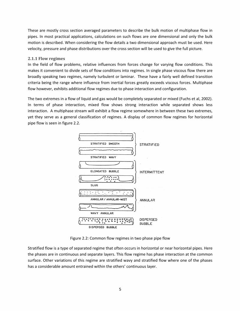
yet they serve as a general classification of regimes. A display of common flow regimes for horizontal
pipe flow is seen in figure 2.2.
Figure 2.2: Common flow regimes in two phase pipe flow
Stratified flow is a type of separated regime that often occurs in horizontal or near horizontal pipes. Here
the phases are in continuous and separate layers. This flow regime has phase interaction at the common
surface. Other variations of this regime are stratified wavy and stratified flow where one of the phases
has a considerable amount entrained within the others’ continuous layer.

6
Annular flow is another separated regime. Here, the liquid covers the pipe walls with a continuous gas
phase inside. Typically the liquid film on the wall is thin and there will be a droplet range in the gas phase
that transports liquid, so called annular-mist.
Bubble flow is when all gas is transported entrained as dispersed bubbles in the liquid. The equivalent
high gas and low liquid flow situation would be gas with a droplet field. However, the droplets will
usually deposit on pipe walls resulting in an annular-mist flow situation.
Some conditions even promote regimes where the flow may have regions of strong mixing followed by
regions of separated flow. This type of flow with intermittent behavior is sometimes referred to as
dynamic flow. Slug flow and elongated bubble flow are two such flows.
Slug flow is the intermittent flow regime where liquid slugs filling the entire pipe cross section are
followed by large gas bubbles. This general description gives a picture of the dynamics; still there are
different slug scenarios with a wide variety in time and length scales.
Hydrodynamic slugging occurs when flow instabilities result in liquid filling the entire cross section.
Starting as stratified flow, a small disturbance on the surface of the liquid may either die out or grow into
a slug. This type of slugging is flow dependent since only flow parameters decide whether or not it
occurs.
With even more phases present, the number of possible phase configurations is higher. Still, a phase will
be transported either as a continuous layer or entrained in another phase, or a combination of both.
Figure 2.3: Common flow regimes in two phase vertical pipe flow (Mishima et al, 1996)
For vertical and near vertical pipes, the mixing forces are very strong. Here, stratified flow can never
exist. All the flow regimes seen in figure 2.3 are mixed flow regimes. Even the annular flow, where a
continuous liquid field may exist along the perimeter, has most of the liquid transported as droplets. The

7
liquid film may even be flowing downwards. For low gas, bubbly flow occurs. Increase of gas flow rate
first leads to slug flow or churn flow and then finally annular flow with mist. In churn flow which is similar
to slug flow, the liquid slugs are almost torn up by gas and the liquid and bubble regions are not distinctly
separated.
2.1.2 Flow regime maps
To know for which conditions the different flow regimes occur is of great interest. Several attempts have
been made to map out flow regimes and the transition between them, but the complexity of multiphase
flow means that it is difficult to make such maps general. A typical way of presenting it is a map where
the different regions can be seen for a given Usl or Usg (Nydal, 2008). A qualitative map in a horizontal or
near horizontal pipe with gas and liquid flow is given in figure 2.4. This shows that the flow regimes are
confined to specific flow conditions.
Figure 2.4: Qualitative flow regime map for horizontal pipes from (Kristiansen, 2004)
The effects of small inclination to the horizontal can be seen. If the pipe is upward inclined, β larger than
zero, the slug flow area is increased. Downward inclination promotes stratified flow. This may be used to
create a certain flow regime in an experimental setting. Increased pressure also affects the map.
Generally, increased pressure will decrease the slug area. This is due to the weight of gas quenching
disturbances, but also that interface forces increase and the gas drags the liquid, avoiding accumulation.

8
Figure 2.5: Flow regimes in vertical and near vertical flows (Johansen, 2000)
In vertical and near vertical pipes with upwards flow, the effect of gravity on the liquid will change the
flow regime map considerably due to mixing forces. High liquid flow rates will give bubbly flow and high
gas gives annular flow. Between these, slug flow is dominant. A qualitative flow regime map for
horizontal and near horizontal pipes is given in figure 2.5.
2.2 Flow assurance – industrial aspects of multiphase flow In the oil and gas industry, the handling of multiphase flow is called flow assurance. This subgroup of
multiphase flow denotes the safe and uninterrupted transport of well stream mixtures in pipelines
(Nydal, 2008). Typically, hydrocarbon well stream consists of water, gas and oil in various combinations,
possibly together with additional contaminants. The focus on multiphase flow in the oil and gas industry
has been motivated by a need to transport unprocessed well stream over longer distances.
Flow assurance encompass much more than the flow related issues. The field is made up of multiphase
flow dynamics coupled with the complex fluid characteristics of hydrocarbon systems. Fluid related
issues include such effects as corrosion, scaling, hydrate formation, fluid characterization and waxing.
However, this thesis will focus on the flow dynamics related effects of a multiphase flow. Important
issues are to predict and control pressure drops and ensure manageable flow conditions.
2.2.1 Slugging
A common challenge in producing fields is slugging. This is the intermittent flow regime previously
described. Not all types of slugging may be a problem. Typically, only so-called severe slugging poses a
threat to production stability (ABB, 2004). Here the large fluctuations in production rates and pressure
may damage equipment or flood the inlet facilities. Slug formation can be caused by a variety of
mechanisms;
Flow effects
Terrain and riser effects
Operational effects

9
Terrain effects are liquid accumulations caused by dips in the flow line or in risers. The resulting slugs
may be very long and can cause damage to topside equipment. Terrain and riser slugging is often
denoted severe slugging.
Slugging caused by flow effects is known as hydrodynamic slugging. In vertical and near vertical flows,
bubbles will travel within the liquid due to buoyancy effects, which results in pockets of gas together
with liquid slugs. Hydrodynamic slugging occurs for a wide range of flow conditions and is therefore
difficult to prevent. However the production rate and pressure fluctuations are usually not very big and
hydrodynamic slugging is therefore not considered severe slugging.
Pipeline operations can also cause slugging. Pigging operations will sweep all liquid out of the pipeline,
which may result in vast volumes of liquid being pushed out into the inlet facilities. Shut down of pipes
means that all liquid will drain into low points, subsequent start up then means accumulated liquid will
travel through the pipes as slugs. Increase in production rate may also lead to a transition from stratified
to slug flow, however, the slug lengths may be longer than anticipated for hydrodynamic slugging
(Kristiansen, 2004).
A common way to deal with slugging that cannot be avoided or severely mitigated is to install slug-
catchers at the inlet facilities. These have a large volume so when liquid enters the facility it will be
temporarily stored so that the inflow to the process plant can still be kept constant and manageable.
However, slug catchers must be dimensioned correctly and issues regarding cost give a need to minimize
the size. With that in mind, it is obvious that an estimate of the size of slugs entering the facilities is
needed. In addition, slugging may become a problem in another phase of production. In this case, if a
slug comes, it will flood the inlet facilities if they have no slug catcher. On floating production, storage
and offloading vessels, it may not be possible to install large slug catchers, so in these cases slugging
must be avoided or mitigated.
Steady production may be important, and severe slugging should be avoided. Due to topography and
that the last part of the pipeline usually follows a near vertical path to the inlet of the process facilities;
terrain slugging is a real concern in many systems with low flow rates and large diameters.
All this adds up to the fact that accurate prediction of slugging is important in many concerns. First it will
determine whether or not slugging is a problem in the system, and if it is, it may be used to dimension
the inlet facilities and the slug catchers. Or the knowledge of the slug problem from the simulations can
help mitigate it.
2.2.2 Terrain slugging
Terrain slugging is a gravity-induced phenomenon and may lead to severe slugging. It happens when a
stratified flow enters a pipe section with upwards inclination. Then, depending on flow conditions,
gravity will cause the liquid to start accumulate in the bottom of the uphill. The following cycles will then
follow one of two possibilities, referred to as terrain slugging type 1 and 2.
A typical terrain slugging 1 cycle starts with a full blockage at the uphill base. The liquid accumulation is
then built up and grows both sides into the uphill section and the flow line. With the full blockage, the

10
upstream gas will start to compress and back pressure builds up. If the volume upstream of the blockage
is big and the compression of the gas slow, the liquid accumulation will be start to drain over the top the
uphill before the back pressure is big enough to move the slug. When the slug starts draining over it is
set in motion, and the back pressure will start to overcome the hydrostatic head. The slug is then blown
out. The resulting slugs may be in the length of 300 – 350 times the pipe diameter (ABB, 2004).
Figure 2.6: Terrain slugging type 1 cycle in straight riser (ABB, 2004)
The last part of the pipeline system taking the flow to the surface and inlet facilities is known as the riser.
The figure below shows the terrain slugging type 1 cycle when it occurs in a straight riser. The blow out is
accelerated as the liquid is drained out the top and into the receiving facilities. The compressed gas
behind it will start to expand, accelerating the liquid plug out of the system. Finally, as the gas has
penetrated through to the outlet some of the liquid will fall back into the dip.
Terrain slugging type 2 is similar to type 1. The main difference is that the back pressure will be high
enough for gas to penetrate into the liquid blockage before it drains over the top. This means that large
gas bubbles will enter into the blockage and float through it. These will push some of the liquid forward
as slugs. However, the slugs and the pressure variations are of a much smaller scale than the ones seen
in type 1. The flow is almost stable, as the back pressure builds up and gas is pushed into the blockage,
when the bubble is pushed in the back pressure will drop it rises again and a new bubble is pushed in.
Terrain slugging far away from the outlet may not always lead to severe slugging. The slugs may die out
before they reach the outlet. The slug frequency is dependent on the upstream compressible volume, it
takes longer for pressure to build up if the volume is large, resulting in longer slugs. This type of slugging
also typically occurs for low gas and liquid flow rates. However, flow in risers will very often pose a risk
for terrain slugging directly into the outlet.

11
To avoid terrain slugging in the pipe system or the riser, it is desirable to have operating conditions
outside of the terrain slugging region. Therefore, stability maps are made to show for which conditions
severe slugging occur. The qualitative stability map below is taken from (Nydal, 2008). These maps also
depend strongly on system geometry and pressure.
Figure 2.7: Qualitative terrain slugging stability map (Nydal, 2008)
It can be seen that the terrain slugging is limited to certain flow condition envelopes. The map is also a
function of certain criteria that must be satisfied for terrain slugging to occur in the system. There are
four criteria:
Downward section with stratified flow upstream
Upward section allowing slug growth
Unstable flow in the upward section
No annular flow in the upward section
Mitigation or complete prevention of severe slugging in the system usually means removing one of these
criteria. If the incoming flow to the riser is slug flow, there will be no large gas volume to compress and
drive the slug out. Instead hydrodynamic slugging will reside in the upwards section. This also means that
the liquid flow rate is sufficiently high to avoid terrain slugging. Slug growth is only possible if the
gravitational forces are balanced against the pressure in the bottom of the riser. This means that if either
the riser is too short, or the pressure high, only small slugs will occur. Unstable flow is when increase in
production leads to decreased system pressure drop, which happens when pressure loss is dominated by
hydrostatic head loss. This is the case for low production rates. With higher production rates, frictional
pressure drop dominates, giving a stable system. Annular flow occurs for high gas rates, if the gas rate is
sufficiently high the liquid will be transported as an entrained component in the gas phase.
2.3 Modelling of multiphase flow Correct and accurate simulation of multiphase flow requires models which take into account both the
flow physics and the fluid related phenomena. In theory, it should be possible to apply the complete
Navier-Stokes set of equations, coupled with appropriate source terms, and solve for all flow parameters

12
in a direct numerical simulation approach. However, to resolve for all the flow complexity would make
this approach too computationally demanding, therefore it is necessary to use other approaches.
Historically, empirical models have been the way to acquire estimates on multiphase flow. Data from
experiments has been used to correlate the structure between the important parameters, for example
pressure drop and velocities. These empirical models are fairly easy to obtain as they do not require
much fundamental understanding. However, the quality of the models will depend strongly on the
availability of data, especially since the data is only measurements which enclose combined effects. And
it has already been argued that the physics of multiphase flow is a complex combination of many effects,
a purely empirical model between important parameters will therefore at best give the correct trend in
flow behavior. Even with these obvious limitations, purely empirical models have been put widely to use
in the past, in the lack of effective mechanistic models (Issa et al, 1988).
In mechanistic modelling, fundamental knowledge of the flow physics is used to define the structure
between parameters (Ming, 2000). A typical approach is to use equations of continuity to get a
mathematical system that can be solved numerically. Since the approach accounts for the interaction
between relevant parameters, the desirable result is a general model suited to give more realistic
predictions.
Still, there are limitations in the fundamental knowledge of certain effects in multiphase flow which
means that at some level, empirical relations are required for closure of the equation sets. Inter-phase
effects such as mass transfer and shear stress will need empirical relations. Flow configuration must also
be implemented; usually the averaged model is solved with a resolution that is not high enough to
resolve for the small variations that causes flow regime transitions (Bonizzi et al, 2009). To know where
flow regime transitions occur is important since the models and relations vary between flow regimes. It
has been argued that the effect of forces changes with flow configuration. A model based on the
influence of a set of forces may therefore not be applicable when the flow regime changes.
In the following, common approaches of mechanistic multiphase flow modelling will be presented. A
typical model is based on transport equations for mass, momentum and energy. This results in a set of
coupled partial differential equations which must be integrated over control volumes. This gives a set of
equations which can be solved numerically. To resolve the fluid related and inter-phase actions, these
must in turn be supplemented with empirical models for friction, chemical effects, mass transfer, heat
transfer and other possible occurrences.
The models will be one dimensional and focused on multiphase flow in a pipeline. If temperature change
is important, the energy equation may be used to model heat transfer in the flow. In many cases
however, the temperature change is not important and the energy equation may be omitted. For the
applications presented in this thesis, the system is isothermal.
2.3.1 The multi-fluid model
An often used method is the multi-fluid model. Here conservation equations are used for each phase
present (Bonizzi et al, 2003). Mass, momentum and energy for each fluid are conserved over a control

13
volume giving a system of equations which can be solved for velocities, pressure, temperature and
phase-fractions.
When applied to a two phase system the resulting set of equations is called the two-fluid model. Mass
conservation for a two phase gas liquid system without sources can be expressed with the following
equations (Nydal, 2008)
( ) ( )
0g g g g gu
t x
(2.10)
( ) ( )
0l l l l lu
t x
(2.11)
These are overall mass balances for each phase and must include both the continuous and entrained
parts. The first term on the left hand side accounts for the accumulation of mass over time and the
second term is the convective transport of mass.
Conservation of momentum for the two phases without external sources can be expressed with the
following equations
2( ) ( )sin
g g g g g g gl gl gw gw
g g g
u u S Spg
t x x A A
(2.12)
2( ) ( )
singl gll l l l l l lw lw
l l l
Su u Spg
t x x A A
(2.13)
The first term on the left is the time rate or transient change of momentum. The second is the change of
momentum due to convective acceleration. On the right hand side, the first term is the phase pressure
gradient. Then comes gravitation and the two last terms are shear stresses. For the gas phase, both the
wall and the liquid will slow the flow down. For the liquid, the wall will exert frictional forces to its
movement. However, since the gas is slowed down by the liquid, the liquid must be accelerated by the
gas, hence the positive sign on the gas liquid shear stress term.
These four equations give a relationship between the velocities, pressure and one of the phase fractions
and can serve as a basis to develop a set of equations which can simulate the transient progress of a
system. In order to solve it, the remaining terms must be known or modeled, and proper initial values
and boundary conditions must be given as input. Particularly, the interface shear stress term can be
difficult to model if velocities are high and there is strong mixing (Issa et al, 2006). This makes this model
less suitable for other regimes than stratified flow.
2.3.2 The multi-field model
The two-fluid model as presented is fit to simulate a stratified flow situation (Nydal, 2008), and then the
shear stress terms between the phases can easily be modeled as they share one large interface.
However, for any other flow configuration it will have difficulties in capturing the physical flow. A phase

14
will often be dispersed and may appear both as a continuous field and as an entrained component in the
other phase. A model which tries to respect the underlying physics is the multi-field model (Bonizzi et al,
2003). In this approach, each field has its own set of transport equations. So in addition to the
continuous fields, the bubble and droplet fields must have transport equations.
A standard one-dimensional two-fluid-four-field model will then use a set of four conservation equations
for each field (Danielson et al, 2005). Since this approach allows for one phase to exist in several fields,
source terms need to be included to allow for mass transfer between them. Mass and momentum
conservation with source terms should therefore be able to model the physics of the different field
combinations.
One application of the multi-fluid model can be found in (Danielson et al, 2005). Here, k denotes one of
the fields continuous gas, continuous liquid, droplet or bubble. Mass conservation of a field can then be
written as
( )k kk k k ki ext
i k
ut x
(2.14)
The left hand side is the same as in the multi-fluid model. On the right hand side there are two source
terms; Γki accounts for the net mass transfer from other fields and Γext is the net external mass source.
There are three modes of mass transfer between fields; mechanical, thermal and chemical. Here the
transfer happens through the mechanical mode with entrainment, disengagement and coalescence. The
other modes encompass a range of effects such as evaporation, condensation, melting, solidification,
solution, dissolution and diffusion processes.
Momentum conservation of field k is
2
int( ) ( ) sink k k k kk k k k k k k k
ki kw ki ki kext kext
i k i k
Pu u g P
t x x x x
F F u u
(2.15)
This equation features two types of pressures, Pk and Pint, representing the average phase and interface
pressures. The term Fki accounts for interfacial momentum exchange with other fields, and the term Fkw
is the frictional force from the wall. The terms Γkiuki and Γkext are the momentum change due to mass
transfer from other fields and external sources, respectively.
By having two pressures, the model accounts for the pressure difference between the phase pressure
and the interface pressure. It takes into account the vertical pressure change due to the liquid height. In
practice the interface pressure will be related to the system pressure and liquid height and inserted back
into the equation.
It is apparent that this model with conservation equations solved for each of the continuous and
dispersed fields should be better suited to simulate all possible flow configurations for a real two phase

15
flow. Finding relations for the source and interface terms is easier now that the modelling is performed
in a more generic manner. For example, instead of having one empirically decided closure relation for
friction between gas and liquid, relations can be found for friction between continuous gas and liquid,
continuous gas and dispersed liquid and continuous liquid and dispersed gas. However, additional
complexity is added as more equations need to be solved. It is not a matter of course that the resulting
set of equations is solvable and some problems regarding instabilities with this model are reported
(Bonizzi et al, 2009).
2.3.3 The drift flux model
Another approach is to regard the mixture of two fluids as one field. This is done in the drift flux model
(Nydal, 2008). Conceptually, this will acknowledge that dispersed fields share some flow parameters with
the continuous field they are travelling within. Therefore the conservation equations may be set up for
the mixture. For a two fluid system of liquid and gas, this amounts to adding together the conservation
equations. The new set of equations is then expressed with mixture variables which in turn must be
related to the fluid parameters.
For the mixture mass and momentum conservation, this gives
( ) ( )0,
,
m m m m m
m m g g l l m m m g g g l l l
u
t x
u u u
(2.16)
2
2 2 2
( ) ( ) 1sin ( )
,
m m m m m mm m m
m m m g g g l l l m gw gw lw lw
u u pg S
t x x A
u u u S S S
(2.17)
As a result of adding together the equations, new mixture variables appear. These can be defined from
the phase variables. In addition, new terms arise in the mixture momentum equation, for example in the
convective acceleration; these are collected in the last term on the right side. The drift flux model also
needs closure relations for the shear stress τm.
If information about the individual fluids in the mixture is needed, these equations must be
supplemented with relations between mixture and individual quantities. These relations are often
algebraic expressions and do not add equations to the set. For the velocity relationship between a
dispersed d and its carrying field m, a typical relation is expressed by constants, or
0 0d mu C u U (2.18)
Thus, the drift flux model uses one set of conservation equations for a mixture of any fluids
supplemented with algebraic relations. Compared to the multi-fluid with uses n sets of equations for a
mixture of N fluids, it is obvious that the drift flux ends up with an equation set less demanding to solve.
However, it is not especially suited for anything but strongly mixed flow.
16
2.3.4 Hybrid models
The multi-fluid and the drift-flux model are both suitable for specific types of flow configurations. The
multi-field model, it was argued, is capable of simulating all types of flow configurations; however the
result is often a very large and complex set of equations. The hybrid approach is to combine the different
models so that all possible flow configurations can be handled (Nydal, 2008), while at the same time
retaining an equation set that can be solved.
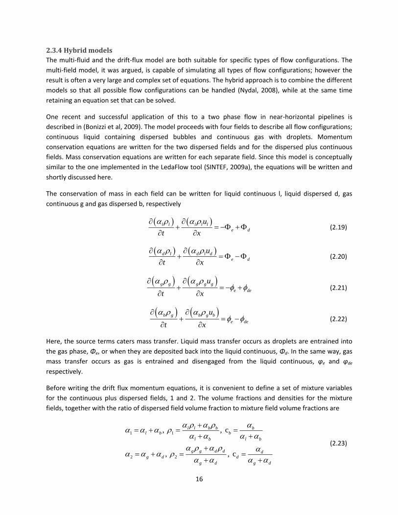
One recent and successful application of this to a two phase flow in near-horizontal pipelines is
described in (Bonizzi et al, 2009). The model proceeds with four fields to describe all flow configurations;
continuous liquid containing dispersed bubbles and continuous gas with droplets. Momentum
conservation equations are written for the two dispersed fields and for the dispersed plus continuous
fields. Mass conservation equations are written for each separate field. Since this model is conceptually
similar to the one implemented in the LedaFlow tool (SINTEF, 2009a), the equations will be written and
shortly discussed here.
The conservation of mass in each field can be written for liquid continuous l, liquid dispersed d, gas
continuous g and gas dispersed b, respectively
l l l l l
e d
u
t x
(2.19)
d l d l d
e d
u
t x
(2.20)
g g g g g
e de
u
t x
(2.21)
b g b g b
e de
u
t x
(2.22)
Here, the source terms caters mass transfer. Liquid mass transfer occurs as droplets are entrained into
the gas phase, Φe, or when they are deposited back into the liquid continuous, Φd. In the same way, gas
mass transfer occurs as gas is entrained and disengaged from the liquid continuous, φe and φde
respectively.
Before writing the drift flux momentum equations, it is convenient to define a set of mixture variables
for the continuous plus dispersed fields, 1 and 2. The volume fractions and densities for the mixture
fields, together with the ratio of dispersed field volume fraction to mixture field volume fractions are
1 1
2 2
, , c
, , c
l l b b bl b b
l b l b
g g d d dg d d
g d g d
(2.23)

17
The velocities occurring in the conservation equations for the mixture fields are centre of mass velocities.
By requiring that the mass flow of the mixture is equal to the sum of continuous and dispersed mass
flow, these can be written
1
1
2
2
(1 )
(1 )
b g b b l l
d l d d g g
c u c uu
c u c uu
(2.24)
Now the momentum equations for the two mixture fields can be written. For the liquid continuous and
gas dispersed field, conservation of momentum may be written as
221 11 1 1 1 1 1
1
1 1
1 1 1
(1 )( ) ( )
sin cos
g l b b s
w wp
i ie l d d e g de b
c c uu u
t x x
SP hg
x x A
Su u u u
A
(2.25)
And for the gas continuous and liquid dispersed field it is
222 22 2 2 2 2 2
2
2 2
2 2 2
(1 )( ) ( )
sin cos
g l d d s
w wp
i ie l d d e g de b
c c uu u
t x x
SP hg
x x A
Su u u u
A
(2.26)
Here, along with the usual parameters, the liquid height h is included. This means that the model
involves the effect of liquid weight on pressure. The subscripts s1 and s2 denote slip between bubbles
and continuous liquid and slip between droplets and continuous gas respectively. The notations Swp1, Swp2
and Si denote the perimeter wetted by mixture field 1, 2 and the interfacial width respectively.
To calculate the velocities of the dispersed fields, momentum equations are written. The dispersed fields
will each have their conservation of momentum equation, which can be written as
2( ) ( )
sinm m m m m mm m m e k de m drag
u u Pg u u F
t x x
(2.27)
Here, m denotes the dispersed fields. Fdrag is the interfacial drag acting on the dispersed field. The source
terms are the entrainment and disengagement from the given field. Momentum contribution from
entrained mass is of course dependent on the velocity it has coming in, which is the velocity in field k.

18
The total system now has eight equations to describe the four possible field configurations. It is now
necessary to model source terms and to include closure relations, these do not contribute to the number
of equations in the set. The required closure in this model are friction factors for the shear stresses and
algebraic equations that gives the mass transfer rates, droplet and bubble size and drag coefficient.
Key elements of the numerical procedure used to solve the equations are pressure-velocity coupling to
get pressure equation, staggered grid discretization, implicit integration of the pressure and explicit
integration for all the other equations. The solution is sufficiently accurate that mass is conserved for
each field.
In (Bonizzi et al, 2009) it is showed that this model is able to give accurate predictions of the flow
regimes and transition between them without changing the closure relations. This implies that the model
is able to capture the flow physics without having to rely too much on closure relations, which should fit
well with the idea behind the LedaFlow project about using generic models and applying closure
relations at lower levels (Danielson et al, 2005).
2.3.5 Slug representation – the unit cell model
In multiphase flow modelling, a common way to represent slug flow is the unit cell model (Nydal, 2008
and Kristiansen, 2004). This is also implemented in LedaFlow (LedaFlow release notes version 2.03,
2009). This is an approximation based on the concept of an ideal slug unit, with a sharp change between
slug and bubble regions. The figure illustrates this with a moving slug with trailing gas bubble.
Figure 2.8: Ideal slug unit in unit cell model (Kristiansen, 2004)
The sharp slug front moves with velocity Uf and the sharp bubble front moves with Ub. The slug is
modeled as bubbly flow with entrained gas represented as average gas void in slug αs. The bubble region
is modeled as smooth stratified flow, with all liquid transport occurring in the continuous layer at the
bottom of the pipe. Parameters in the bubble region are Ugb, Ulb and αb. The length distribution between
slug and bubble, Ls and Lb, is contained in the slug fraction parameter, Sf.

19
sf
s b
LS
L L
(2.28)
In all, the unit cell slug flow model constitutes nine parameters which describe an average and ideal slug
unit moving with velocity Uf. These need nine equations, of these the void in slug αs, bubble front
propagation velocity Ub and slug length Ls need empirically decided equations, the rest may be solved
from stratified and bubbly flow models and from considering continuity inside the slug unit.
2.3.6 Closure models and empirical relations
In order to obtain closure to the equation set developed in the model it is necessary to find expressions
for the source terms. The source terms for shear stress, mass transfer and drag in the momentum and
mass equations must all also have their own models.
The interface and wall shear stresses are typically modeled with friction factors. The wall shear stress felt
by field or phase k is then (Bonizzi et al, 2009)
1
2wk wk k k kf u u (2.29)
For large interfaces between continuous fields, the shear stress is also modeled as a function of friction
factors, but now the relative velocity must be used. For example between a gas and liquid phase
1
2i i g g l g lf u u u u (2.30)
The friction factors are given by empirically decided correlations. These are typically functions of the
Reynolds number and the hydraulic diameter, which depend on flow variables, fluid properties and flow
geometry. For non smooth pipes or wavy interfaces, roughness height approximations apply. The
Reynolds number and the hydraulic diameter for field or phase k are
4
Re , k k k kk k
k k
u D AD
S
(2.31)
For dispersed fields, drag forces may be used to describe the resistance felt from the surrounding field.
The drag force on bubbles or droplets is often expressed as a function of the relative velocity and the
drag coefficient. The drag coefficient is typically a function of size of the dispersed particles. Empirical
relations for bubble and droplet diameter must therefore also be provided.
Drag force on a particle dispersed in field k can be given in terms of the drag coefficient CD, relative
velocity ur and projected area Ad of particle (Ishii et al, 1979).
1
2drag k D r r dF C u u A (2.32)

20
Other types of terms that need closure are mass transfer terms such as entrainment, disengagement and
deposition rates. These terms are often given as empirical expressions of fluid properties and flow
variables. A relation for the droplet deposition rate Φd for example, is given as (Bonizzi et al, 2009)
4 d
d d l
g
kD
(2.33)
In addition to this, flow regime transition models are required. The multi-fluid multi-field model
presented earlier was able to predict this as part of the calculations however this required a very fine
grid and a complex model. For other implementations, flow regime transition occurs when a given set of
conditions are met. For slug or non-slug flow a common approach is to use existence of slug flow as the
criteria. According to the unit cell model, if Sf is between 1 and zero, slug flow exists. If Sf is above 1, it
suggests bubbly flow, and if Sf is below zero it suggest a separated regime, either stratified or annular.

21
3 Experiments on gas-liquid flow in an S-shaped riser In spring 2000, air water experiments on a flow line and riser system in the multiphase flow lab at NTNU
were performed (Johansen, 2000 and Nydal et al, 2001). A downward inclined flow line was combined
with an S-shaped riser. This setup is often seen in real off shore producing fields and is associated with
slugging. The fluids were water and air at ambient conditions. Experiments were carried out with a
variety of flow rates and the results were used to create stability maps and for comparison with an in-
house programmed simulation tool for slugging. The objective was to supply experimental data on
multiphase flow in S-risers and compare this to models.
3.1 Instrumentation and setup The flow loop was constructed using PVC pipes mounted to the wall. The total height of the S-riser was 7
m and the inner diameter of the pipes 5 cm. Presence of liquid was measured with impedance probes at
three locations. Transformation to holdup values was not possible as the impedance probes had not
been calibrated, however in this text they will be referred to as a measure of holdup. Four fast absolute
sensors were used for pressure measurement. The setup together with the instrumentation is shown in
the figure below. Instrumentation indicated with P for pressure sensors and I for impedance probes.
Figure 3.1: Experimental setup (Johansen, 2000)
To simulate a larger upstream volume, a tank was inserted between the gas control valve and the gas-
liquid mixing section. By adjusting the water level in the tank, upstream volume could be made
equivalent to 167 m of pipe length. Limited space in the lab would otherwise constrain the experiments
since having a large upstream volume is important for the wanted flow dynamics.
3.2 Slugging observed in the experiments In the experiments, slugging occurred for all flow rates. For the largest upstream volume, 167 m of
equivalent pipes, both terrain and hydrodynamic slugging were observed. The results from these

22
experiments are discussed in the following. In the end a stability map was made based on the types of
slugging at different flow rates.
Terrain slugging type 1 in the S-risers follows the same cycle. The liquid in the stratified flow in the flow
line will start to accumulate leading to a full blockage of the first bend at the riser base. This blockage will
grow as more liquid is accumulated, meanwhile back pressure increase as the upstream gas is
compressed. Often the dip will already be liquid filled due to backflow from the last slug cycle. The gas
trapped between the two blockages will also be compressed as the liquid column in the first riser grows,
but usually not enough to blow out the blockage in the dip. When the liquid column in the first riser
reaches the riser top, the liquid will immediately drain into the dip as stratified flow. Now the blockage in
the dip also grows until finally it reaches the riser top, at this point the blockade fills parts of the flow line
and the entire riser except for a gas bubble from the trapped gas.
When the liquid starts flowing out the top, the entire blockage will start to move. When the gas front
reaches the riser base, the gas will start to penetrate the liquid and the hydrostatic pressure decrease
both as liquid is drained out and gas is mixed into it. As an effect, even more gas penetrates into the
liquid until finally the upstream gas is able to expand and push the slug out. The effect of decreased
hydrostatic pressure and expanding gas is an acceleration and blow-out of the blockage which is now
torn into smaller slugs and bubbles. At the outlet, the blow-out process starts with the slug from the
second riser, and then this is followed by the trapped bubble which in turn is followed by the slug from
the first riser. After this a tail of small slugs and bubbles flows through the system. The cycle is
repeated as new liquid starts to accumulate in the bend. Also, the dip is filled by back flow from
the blow-out process.
Figure 3.2: Inlet pressure during terrain slugging type 1 (Nydal et al, 2001)
Figure 3.2 show the pressure time series for a typical type 1 cycle. Inlet pressure increase as the blockage
grows. For a very short time, the pressure is constant while the slug starts to move. This is followed by a
sudden expansion as the gas front reaches the riser base and the slug is blown out. In this case, build-up
of the blockage and pressure takes approximately 40 s, and the subsequent blow-out about 10 s. The
inlet pressure varies between atmospheric conditions up to about 1.75 bar, the pressure variations are
thus in the size of 0.6 bar.

23
Figure 3.3: Holdup at the top of the first riser and at the outlet (Nydal et al, 2001)
Holdup time series for the cycle are shown in figure 3.3. The first depict holdup at the top of the first
riser and the second shows the outlet. A period of zero holdup at the top of the first riser occurs before
the blockage has grown into the top. Then, large slugs are blown out followed by smaller slugs and
bubbles. At the outlet, holdup equal to one occurs for a shorter period than at the downstream position.
This is because immediately after the liquid blockage reaches the top, the blow-out process starts. It may
seem like the holdup is never zero at the outlet, considering this is the steepest part of the riser this is
more likely to be due to the lack of calibration or that a liquid film remains on the walls due to backflow
from the outlet.
Figure 3.4: Pressure difference between inlet and riser base (Nydal et al, 2001)
In this figure it is seen that pressure difference is negligible during blockage build-up. This would imply
that there is still stratified flow in this section. When the blow-out occurs the pressure drop has
fluctuations. These indicate slugs in the flow line due to gas acceleration.
Terrain slugging type 2 occurred for higher gas loading. This type of slugging happens when the back
pressure is able to push gas into the liquid blockage. This leads to smaller slugs being formed. As the gas

24
enters the blockage at the riser base, buoyancy will let it move through the almost stagnant liquid
column.
Figure 3.5: Inlet pressure terrain slugging 2 (Nydal et al, 2001)
The result is a more stable slug flow. Figure 3.5 shows the inlet pressure time series for this type of flow.
There are fluctuations, but they are generally faster and a lot smaller than for type 1 slugging. The
maximum amplitude in this series is for example somewhere around 0.15 bar. During 200 seconds of
type 2 terrain slugging, around 14 distinguishable pressure tops can be seen, compared to the 4 distinct
cycles of type 1 seen for the same period.
Figure 3.6: Holdup for terrain slugging 2 (Nydal et al, 2001)
The resulting slugging is seen in the holdup time series in figure 3.6. At the top of the first riser, some
periods of liquid accumulation in the riser base can be seen as holdup is zero. Holdup values at the outlet
will also fluctuate, but here no periods of upstream blockage can be seen. Generally, the slugging in type
2 is faster than type 1, therefore the pressure and holdup variations are correspondingly smaller which
makes this type of flow easier to handle at the outlet.
Steady slugging was also observed in the experiments. This is hydrodynamic slugging and occurs for
higher gas or liquid flow rates.

25
Figure 3.7: Inlet pressure for steady slugging and terrain slugging 2 respectively (Johansen, 2000)
The inlet pressure and holdup time series for this type of flow showed very fast fluctuations. It is easier
to see the difference between steady and terrain slugging type 2 by comparing the plots in figure 3.7.
Inlet pressure with steady slugging is to the left, it is clearly seen that here the pressure fluctuates faster,
but with smaller amplitude. While the plot to the right clearly shows the build-up periods of terrain slugs,
the one to left show no clear build up of pressure over a longer period.
Figure 3.8: Holdup at top of first riser for steady and terrain slugging 2 respectively (Johansen, 2000)
Comparing the holdup time series at the top of the first riser helps distinguish steady slugging from
terrain slugging type 2. It can be seen that the steady flow continuously have medium fluctuations on the
holdup but never zero holdup, which indicates that both gas and liquid flow through at all times.
Sporadic tops show that some slugs are longer than others. The terrain slugging type 2 at the first riser
top however shows that the holdup is zero at some times, which indicates sporadic slug build-up.

26
Figure 3.9: Holdup at outlet for steady slugging (Johansen, 2000)
Holdup time series at the outlet shows that the flow structure is retained through the riser. Also here,
fast fluctuating holdup indicates steady slugging.
3.3 S-riser stability map The experiments were conducted at a variety of flow rates, and a stability map was determined. Since
the definition of flow type was based on a combination of visual inspection of pressure time series,
standard deviations of the inlet pressure and visual observation of the flow during experiments, it is
stated that certain subjectivity is inherent in the maps, in particular for higher gas flow rates (Nydal et al,
2001). The prevailing flow regime in these experiments is different modes of slug flow. In these
experiments it is only distinguished between stable slug flow and modes of terrain slugging.

27
Figure 3.10: S-riser stability map (Nydal et al, 2001)
The trends in this stability map agree well with the other stability maps and terrain slugging criteria
discussed in chapter 2. The map shows that terrain slugging 1 is confined to a limited envelope of flow
conditions with low gas flow rate. Terrain slugging 2 is also confined to a certain region, while steady
slugging is the typical flow regime. It is probable that annular flow would be achieved at higher gas rates
and that bubbly flow would be achieved at higher liquid flow rates.
3.4 Previous simulations on the S-riser Some research has previously been done on how simulation tools handle the flow dynamics of the S-riser
case. In (Johansen, 2000) OLGA simulations are done on one of the terrain slugging type 1 cases, the one
with 2.2 m/s usg and 0.32 m/s usl. A PVT table with water and nitrogen was used. The S-riser was
implemented as a simplified geometry with sharp bends. The results showed that OLGA was able to
predict the correct pressure and holdup time series trends. The inlet pressure plot showed that slug
periods were longer and pressure amplitudes were higher, but in the same range as the experimental
results. The holdup time series did not show the trailing gas and small slugs that followed each blow-out
this is because OLGA treats this as slug flow and only gives out averaged values Johansen argues. The
departures are assumed to be due to coarse discretization of the simulation grid and large time steps.
In (Nydal et al 2001), a slug capturing model was used to simulate the S-riser flow. The computations
were made with the same geometry as Johansen and slug were initiated in bends. An ideal gas state
equation was applied for the air and the water was considered incompressible. Terrain slugging type 1
was successfully predicted for a case with usl at 0.32 m/s and usg at 2.23. The inlet pressure showed the
correct build-up amplitudes and periods. The holdup time series show that the simulations are able to
capture the blow out of the large slug and the trailing bubbles and small slugs. Terrain slugging type 2

28
was also successfully predicted for a case with usl 0.3 m/s and usg at 4.1 m/s. It is more difficult to
compare the time series for this type of flow, however, inlet pressure showed that results are
comparable in terms of pressure value and slug frequency. Holdup time series also showed comparable
results. An analysis comparing inlet pressure oscillation periods showed that the model was able to
predict the transitions between the different types of slugging.
In (Andersen, 2007), the S-riser case was tested in LedaFlow 1.05, and earlier version of LedaFlow. The
same geometry as in the other simulations was used. However, fluid properties were assumed to be
constant. This holds for water, but for the air, compressibility is essential to get severe terrain slugging. A
selection of cases that gave terrain slugging in the experiments were simulated, but the simulation
results did not imply any severe slugging for any of them.

29
4 LedaFlow and the LEDA project LedaFlow is a new multiphase flow simulation tool for design and analysis in oil and gas operations. It is
currently under development by the LEDA partners SINTEF, TOTAL and ConocoPhillips. The LEDA project
vision is to become a “Technology leader in simulation and prediction of multiphase flow – wells,
pipeline and process facility” (SINTEF, 2009b). With LedaFlow, they seek to achieve a step change in the
advancement of multiphase flow modelling. The LedaFlow software suite will be specialized for
simulation of hydrocarbon multiphase flow by having
A transient tool with 1D, 2D and 3D models
Models that are supported by existing and new data from the SINTEF multiphase flow
laboratory, and data from the other LEDA partners
In 2008 the LEDA partners went into a Term sheet agreement with Kongsberg Maritime on possible co-
operation on commercialization of the LedaFlow technology (Kongsberg Maritime, 2008). The tentative
release of LedaFlow services in the oil and gas market is to be in 2009 – 2010 (Kongsberg Maritime,
2009) through the new business unit Kongsberg Oil & Gas Multiphase Flow Solutions. In the first period,
consulting services with LedaFlow will be offered, before the launching of a stand-alone engineering tool
which planned in 2010.
4.1 Background The background of the LEDA project was future challenges seen in the oil and gas industry, where new
and existing projects were having more complex production (Danielson et al, 2005). As a result, there
was a need to develop more accurate transient multiphase flow simulation tools for flow dynamics and
flow assurance aspects. Therefore, in 2001 SINTEF and ConocoPhillips decided on a 10 year research and
development program subdivided into three phases. The following year, 2002, TOTAL joined in and the
first phase of LEDA was initiated as a joint industrial project.
In the first phase, which lasted from 2002 to 2004, the focus was on establishing a new mechanistic
modelling foundation. To support the model, extensive and large scale flow tests were done in the
SINTEF multiphase flow laboratory. It was also important to demonstrate that the new modelling
concept could achieve equal or better performance than existing models. Existing data from the SINTEF
laboratory together with field data were used to demonstrate the model’s capabilities.
In phase two, the goal is to have a fully working engineering tool with a 2- and 3-phase 1D and 2D model
(Q3D). Further experiments were performed to support the development, now with emphasis on 3-
phase systems. In the third and last phase, LedaFlow should exhibit multi-dimensional capabilities
coupled with flow assurance modules that takes into account complex fluids, complex geometries and
wells. It should have an interface towards other process simulation software such as Kongsberg’s own K-
spice suite. The step change is to have the flow assurance issues correctly implemented together with a
3D model for the local flow assurance. This should sit on top of a solid 1D model.

30
Figure 4.1: LEDA project ambition (LedaFlow users’ manual, 2009)
4.2 LEDA status The newest version of LedaFlow is the 2.06 release which came in June. At present the modelling
capabilities in this version are
2- and 3-phase 1D transient model – predicts multiphase flow in any pipe geometry
2- and 3-phase 1D point model – steady state solutions
2D model (Quasi 3D) – computes a quasi three-dimensional representation of the flow
The Q3D model is there to give a more detailed insight into the flow. Width sectional averaging of full 3D
equations gives a 2D model for the variations over the vertical plane. These can be extrapolated back
into 3D, giving a quasi 3D model, the Q3D. It can be used as a looking glass at critical points. Trials have
shown that it gives results in very good correspondence to experimental data (Laux et al, 2007).
Together the 1D transient and point model make up the workhorse of the LedaFlow tool. It is with these
models that 80 % of the multiphase analysis will be done (LedaFlow users manual, 2009). These models
are still under development, and must be thoroughly validated against available experimental and field
data. In this work, these 1D models will be tested against a set of cases from an experimental campaign
on terrain induced slugging. Therefore, the following will give a brief overview of the LedaFlow 1D
module.
4.3 LEDA 1D module The approach in the LEDA project is to improve the accuracy and scale-up capability of the simulation
tool by including more fundamental physics, rather than relying on empirical models (Danielson et al,
2005). The idea is to create a fundamental physical model with a numerical framework that is able to
simulate all possible situations.
The current content of the LedaFlow 1D module are
Steady state point model
Transient and fully compressible 1D model
Flow regimes: bubbly, slug, stratified, annular, mist
Full thermal and compositional tracking

31
2-, 3- and 3-phase with sand
Cut and paste from excel
Input by scripts or GUI
Plotting and visualization in the GUI
This thesis will focus on the 2-phase model, and the GUI will be used to build and manage cases. Thermal
and compositional tracking will not be activated.
4.3.1 Multi-fluid multi-field approach
This chapter will seek to present the 1D modelling-approach and how it is implemented.
In multiphase systems, each phase will typically appear in different forms. Consequently, the phase
behavior changes depending on what form the phase is in. A phase may appear as continuous or
entrained in other phases. This is why, in the LedaFlow model, all materials which exhibit the same
thermal properties are treated as an individual fluid. In a pipeline system, a fluid mixture may consist of a
number of different fluids and materials, such as; gas, oil, water, sand, hydrate, wax or other
compounds. The description of the motion of one such fluid is called a field. Wax and hydrates are also
treated as fluid with fields describing their motion. Sand movement is described as particles.
For a system of three phases in the LEDA model, up to nine fields may be present; three continuous and
six dispersed. Figure 3.1 illustrate a possible configuration o these nine fields. Each of these fields must
then be described by volume fractions, field velocities, enthalpy, particle size in case of bubbles and
droplets, physical properties, temperature and composition. To find these, a set of conservation
equations are used. This approach is referred to as a multi-fluid multi-field model and has been
presented in chapter 2.
Figure 4.2: Three phase system with nine fields; three continuous and six dispersed
It has already been argued that this modelling approach enables all possible flow situations by having
fields for each possible configuration. There are two possible concepts that can cater for this; the multi-
fluid and the multi-mixture, referred to as the hybrid approach in chapter 2. The former gives 9 fields and
9 sets of coupled conservation equations, it is already mentioned that this gives challenges to numerical
method regarding stability and convergence. The multi-mixture uses conservation of mass and energy in

32
each field, but uses momentum equations for the continuous plus dispersed fields, 3 fields that is. This
gives fewer challenges to the numerical issues.
The key concepts of 1D modelling in LedaFlow can be summarized as
Multi-fields to describe the n phases
Possibly n continuous and (n-1) × n dispersed
Mass and energy equations for every field
Momentum equations coupled with drift flux model for the continuous plus dispersed fields
The flow regimes in the present 1D version of LedaFlow are stratified, annular, bubbly flow and slug flow.
The stratified regime assumes flat surface and that each zone can contain dispersed masses of the other
phases. For upwards inclined pipes, annular flow may occur. The bubbly flow is continuous liquid with
bubbles. In slug flow the unit cell model is used. This means that the flow in the slug is bubbly flow and in
the bubble, stratified or annular.
Flow regimes in LedaFlow have continuous transitions. In flow regime determination, the basic criterion
is if slug flow is possible or stable, slug flow exists. If not, it tests for other flow regimes. Since LedaFlow
uses the unit cell model to describe slug flow, this implies slug flow if the slug fraction Sf is found to be
between 0 and 1. It is assumed that this criterion is more appropriate for high pressure systems than for
low pressure ones.
The 1D point model is a module in the framework which computes steady state solutions for the flow,
given a set of input conditions. By giving it pipe data, flow rates and phase data it gives as output the
steady state field volume fractions and velocities, pressure gradient and flow regimes. It is used in other
modules as a resource to initialize, supply flow regimes and friction terms. Since the point model is called
from the transient model at every time step to supply flow regimes, it is extremely important that the
point model is both fast and robust.
The numerical implementation of LedaFlow is also confidential. The solution process however has been
made available by SINTEF and it can be described by the solver flow chart seen in figure 4.3. First it
initializes and sets up the mesh and node points. Then the calculation at one time step may begin. It
starts by preparing each pipe, by computing all fluxes and values needed from the last time step or
initialization. Then the momentum equation is prepared by computing all needed terms and boundary
conditions before the momentum equation matrix and residual are built with boundary conditions. This
is solved by a matrix solver, the solution is updated and values are communicated to the nodes. Then the
mass, volume and pressure equations are to be prepared and solved. First all terms and boundary
conditions must be calculated, then the matrix is built and finally solved. The solution is updated and
values are communicated to nodes. At this point, it checks for convergence with last iteration. This runs
till the mass, volume and pressure solutions have converged for the given solution to the momentum
equations. If the mass, volume and pressure solution is converged it proceeds to solve other equations
such as the energy equation. If these do not converge, the momentum equation is solved again with
subsequent convergence of mass, volume and pressure. Finally, the solution of all equations at the time
step is converged and next time step may begin.

33
Figure 4.3: LedaFlow solver flowchart (SINTEF, 2009a)
4.4 System structure and user functionalities The typical structure of LedaFlow is composed of three main parts (LedaFlow users manual, 2009); the
Leda client, server and a database for storage. This means that to use it, the computer needs to be
connected to the Leda server and the database. In this work, a stand-alone version has been installed on
a laptop, so the system structure is somewhat different. Most importantly, LedaFlow can be run without
being connected to the server or database.
System structure for stand-alone is the LedaFlow client for setting up cases, running calculations and
analyses of results. The data is then stored locally and for every case running, a new Leda “server” is
running in the background on local resources. Input to the client is given through a graphical user
interface called Zeus. This allows for setting up and managing cases in a fast and straight forward way.
The current graphical user interface, from LedaFlow version 2.06, is shown below.

34
Figure 4.4: Graphical user interface, GUI, of LedaFlow version 2.06
The GUI uses 5 windows, the case browser, inspector, property editor, status and the frame window. In
version 2.06 there are also two toolbars, on the left side and on the top side. In the one on the left side,
there are icons for the validator, network viewer, geometry and mesh, library, plotting, 3D visualization
and script editor. On the top side, important case management icons such as settings, purge, start, stop
and initialize are placed. New cases can be built in the GUI, imported from script files or from OLGA
cases.
Building a case in the GUI is done by creating a new case and selecting type of model. In version 2.06 the
case types are either 1D 2- or 3-phase or Q3D 3-, 2- or 1-phase. Then, the geometry must be imported to
pipe settings. Here, pipe co-ordinates, diameter, roughness height, temperature, heat coefficient and
type of wall must be specified. The next step is to define mesh in mesh settings, typically the user
specifies number of cells and then the cells are distributed automatically. It is also possible to manually
distribute or import a mesh from file. In the network viewer, node types can be changed and equipment
can be added. Available items are valve, source, well and dynamic well.
In case settings much of the important input values can be set. Under model options, PVT option can be
set to constant values, imported PVT file or Guts. The latter is a PVT database owned by ConocoPhillips
which may be used in the future versions of LedaFlow. Other options here are energy option,
compositional tracking and mass transfer models. In flow settings, boundary conditions at node points
can be set. At the inlet, which is typically a constant mass rate node, flashing can be turned off and

35
temperature and mass flow rates with mass fractions must be given. At the outlet, typically constant
pressure, pressure must be given. If a source or other devices are added to the pipe, the device settings
can be used to define input to these. All input values can be given at specific time points if transients are
wanted. In numerical settings, simulation time and sample rate is set to control simulation time and
output rate, CFL and maximum time steps are set to control time steps.
The time to advance the solution that is chosen is how many real-time seconds the calculation should
proceed. It starts from the last data stored, which means a simulation can be stopped and started at any
point without affecting the result. This is especially convenient if the simulation crashes, then the purge
functionality can be used to delete some of the last data, and the simulation can be restarted from there
with lower time step size.
Time step size refers to the time interval used to integrate the equations between two time points. In
LedaFlow, the size of these time steps is a function of the results at the last time step. This dynamic
approach lets the time step adjust to how fast the variables are changing; if things are happening very
fast, the time step must be reduced. The time step size is calculated using (LedaFlow users manual,
2009):
,
,
min , *minU
imax
k ik i
xt t CFL
u
(4.1)
Where Δtmax and CFL are user specified. Thus, the user can decrease these values in case of stability
problem. For example in a severe slugging case, during the blow out variables are changing a lot faster
than during the build-up. Typically, the simulation will crash when going from build-up to blow-out.
Purging a few steps back and decreasing these parameters may let the simulation calculate the blow out
sequence. Since sample rate, which is the rate data is extracted from the calculations to output, is also
user specified this can in effect also be used to lower the time step size. If the sample rate is set lower
than the actual Δt, LedaFlow will use the smallest.
In LedaFlow, there are default values for all simulation parameters. This means that even if the user does
not specify all of the required input values, the simulation will still run based on the default values. This
makes it very easy to set up cases, since much of the default values are applicable to most cases.
However, it may lead to confusing results if input values are forgotten.
Simulation status and progress can be seen in the status window. In the output pane, messages from the
calculation are given, such as warnings or error messages when it crashes. At the start of every
simulation it states which models are run, and at the end of simulations it writes out the time it spent
and that the simulation is finished. Output from simulations can be seen in plotting. Here both base and
derived results can be plotted and updated while the simulation is running. The actual data can be
accessed in the inspector and property editor window. Here, either time series in cells or profile series
are given for all results and can be copied into excel. It is also possible to monitor the error in the
calculation; residuals and errors from volume, mass flux, pressure correction and momentum calculation

36
are given. If a simulation runs astray, it may be possible to see, for example, at which time step it failed
to have sum of mass fluxes to be zero.

37
5 Simulation To test LedaFlow’s capabilities on the low pressure air water system, a number of simulations have been
performed. The following will describe the simulation set up and input parameters.
In the experiments, different types of flow were seen for different conditions. The cases will therefore be
divided into three simulation sets accordingly; experimental terrain slugging 1 (ET1), experimental
terrain slugging 2 (ET2) and experimental steady slugging (ESS). In the outset, how LedaFlow handles the
severe slugging in ET1 and ET2 is especially interesting. The so called steady flow in ESS also exhibit
sudden and stochastic fluctuations which must be handled and resolved for. Running all cases will also
give a picture of the robustness and accuracy for different flow rates, and show where LedaFlow predicts
flow regime transitions.
Figure 5.1: Simulation sets ET1, ET2 and ESS
Since LedaFlow is in development, new versions are being released continuously. During this report, four
official versions have been released; 2.03, 2.04, 2.05 and 2.06. Most of the cases in every set have been
simulated in all versions and results have been communicated back to the developers. Significant
improvements had been made to the slug handling in the last release, so the results from this will be
emphasized.
Version Date
2.07pre June
2.06 June
2.05 April
2.04 March
2.03 March
Table 5.1: LedaFlow releases
0
0.2
0.4
0.6
0.8
1
1.2
1.4
0 0.005 0.01 0.015 0.02 0.025
Ml -
kg/s
Mg - kg/s
ET2
ESS
ET1

38
The 2.06 release turned out to have a bug regarding the flow regime transitions. So, SINTEF put together
a preliminary compilation of the next version with the bug fixed. This is called version 2.07pre here, it is
something between 2.06 and 2.07, really more of a version 2.06 plus. Since this version came very late in
the process, only a selection of cases is simulated with it, still the results from these will be emphasized.
5.1 Simulation purpose Before specifying any inputs, it is important to have an idea of what the results should demonstrate. In
this work, the aim is to demonstrate LedaFlow’s capabilities on the S-riser case regarding
Accuracy
o Prediction quality
o Result quality
Numerical behaviour
o Robustness – simulation output
o Stability – simulation progress and application behaviour
o Efficiency – computation time
o Grid dependency – mesh sensitivity
Accuracy can be demonstrated with results that compare well to experimental data. To obtain accurate
results, it may be relevant to change simulation settings to see which factors lead to coincidence
between experimental and simulation results. Robustness relates to if the tool is able to give out results
for any reasonable input to a case. Here, the quality or accuracy of the results is not important. A
correctly set up case should be able to give out results regardless of the input values. Stability relates to
how the tool functions and how the simulations progress. If the application crashes or simulation results
go astray or crashes, this will be poor stability. Efficiency will be demonstrated by simulation time; for
converged solutions, LedaFlow gives CPU time as output. Finally, grid dependency will be tested by
comparing results from simulations with different meshing.
5.2 Base case All cases will first be simulated in a base case. In doing so, it will be easier to compare results from
different cases. It also gives an idea of how LedaFlow responds when one case is run with a wide variety
of flow rates. The typical outputs of a base case simulation are the inlet pressure time series, outlet
volume fraction time series and flow regime index. In LedaFlow, one base case will be built and then it
can be duplicated and given proper input values for any one of the test cases. This should rule out any
idiosyncrasy due to case specification in the results. In running all cases with the same set up,
robustness, stability, accuracy and efficiency should be demonstrated.
5.2.1 Geometry
A representation of the S-riser geometry has been obtained from previous simulations (Nydal et al,
2001). There, the OLGA tool was used and the geometry had to be represented by pipe sections. This
resulted in a simplification of the geometry. The figure below shows the geometry used in the previous
S-riser simulations, also the one in LedaFlow version 1.05 (Andersen, 2007).

39
Figure 5.2: Simplified S-riser geometry with sharp bends
The upstream volume is implemented by a 167 m inclined pipe section with inner diameter 0.05 m. This
gives the correct total volume of the system. Physically, the extra length means a higher frictional
pressure drop. However, since the calculations from OLGA (Johansen, 2000) and slug tracking model
(Nydal et al, 2001) showed relatively accurate results it is assumed that this simplification may be
reasonable. Calculation wise, the extra pipe length requires more calculation time since the control
volumes along the pipe must also be solved for.
Since previous simulations with LedaFlow using the simplified riser with sharp bends did not give
accurate results (Andersen, 2007), another representation of the riser will be introduced here. The tank
is modeled as a pipe section with increased diameter. The bends are smoothened to be more similar to
the actual geometry. Some of the previous work had the water source placed together with the gas inlet.
Here, air is flowing in to the tank at the inlet and a water source is placed at the correct position just
after the buffer tank. To avoid water back flow into the tank, it is placed vertically. The outlet must also
be slightly tilted to avoid back flow. The result is a more accurate representation of the S-riser and tank
geometry, as seen in the figure below.
0
1
2
3
4
5
6
7
0 50 100 150 200
y - m
x - m

40
Figure 5.3: Smooth S-riser geometry
Geometry is imported to LedaFlow by filling in pipe settings in the geometry editor, this can be done by
copy and paste from an excel sheet. X, Y and Z coordinates are inserted together with diameter and
roughness height. Since the S-riser system is a purely hydrodynamic problem, temperature, wall
conduction factor and wall type may be left at default values.
5.2.2 Roughness
In the original laboratory set up, PVC pipes were used to create the S-riser, but there are no information
regarding the roughness. Wall roughness of PVC pipes is not readily obtainable and the actual roughness
will vary between producers. The OLGA and slug capturing simulations used a roughness of 10 μm (Nydal
et al, 2001 and Johansen, 2000), and the LedaFlow simulations used 20 μm (Andersen, 2007). However,
other sources suggest a lower roughness height. In addition, initial simulations in LedaFlow had problems
with cases that crashed due to very large velocities which may have been caused by too low shear
stresses. To try to avoid this, the base case will be set up with a roughness of 2e-5 m. This is also because
it is assumed that the roughness height does not affect the results much. A brief sensitivity analysis
regarding roughness will also be performed.
5.2.3 Meshing
In LedaFlow, the meshing is set in the Mesh settings. Here, section mode is used to distribute a chosen
number of cells automatically. The chosen number of cells in LedaFlow is in reality number of cell faces.
When choosing a mesh of 50, 49 cells will be used. Control points are set at first and last point. A high
number of cells are required to obtain the same accuracy in the geometry used in simulations as in the
imported geometry. However, this would slow down the simulation speed and might cause instabilities.
Therefore, a number of cells that both represent the imported geometry precisely and gives satisfactory
simulation performance should be used.
0
1
2
3
4
5
6
7
8
0 2 4 6 8 10 12 14 16
y -
m
x - m

41
The effect of cell number can be seen both on the actual heights and total volume. Liquid column heights
affect the pressure profiles. Since compressibility is an important factor in the S-riser system, total
volumes must also be close to the real geometry.
Mesh # Total volume - m3 Deviation
15 0.397395 8%
30 0.385511 5%
50 0.372779 1%
100 0.369546 0%
200 0.367954 0%
Table 5.2: Total volumes of geometries
If it is assumed that a mesh of 200 to describe the system gives something very close to the real total
volume, it is seen that deviation from total volume generally decrease as number of cells increase. At 50,
it seems as if the automatically generated mesh fits the real geometry.
Figure 5.4: Effect of meshing on height
This figure shows the effect on the heights. All three does give the correct heights. The one with 30 gives
sharp bends. Also, the upwards inclined pipe into the outlet may cause trouble with back flow from
outlet. Mesh number of 100 gives a very smooth geometry, however the calculation time is very high.
The one with 50 seems to give a reasonable approximation of the geometry, included the smoothed
bends.
The number of cell faces is set at 50 in the base cases. This gives a precise representation of the
imported geometry and experience shows that it still retains decent simulation time.
0
1
2
3
4
5
6
7
5 7 9 11 13 15
y -
m
x - m
1005030

42
5.2.4 Input and initialization
Building a new case in LedaFlow is quickly done once the correct geometry and PVT files are in place. In
all versions, the S-riser case is built as a Leda 1D – 2 phase case. In model options, energy option,
compositional tracking and mass transfer are turned off. The PVT option is set to PVT table and an air
water table is imported. The PVT table used is supplied by SINTEF. The pressure range is 0.5 – 10 bar,
which should be enough for the S-riser.
The water inlet is modeled as a source at pipe length around 7 m, and then this is inserted in the
network viewer. In flow settings, a constant mass flow inlet and constant pressure outlet is chosen as
boundary conditions. At the inlet, total mass flow rate and mass fractions are set, flashing is turned off.
This means that total mass flow rate is set at total air rate, and mass fractions are set to only have gas in
the inlet. The outlet is set to 1 atm. At the source, liquid phase mass flow is set to the water mass flow.
The precise location of the source on the mesh can also be checked, it should be placed directly after the
tank outlet. All temperatures are set at 280 K. The resulting system can be seen below.
Figure 5.5: Inlet, water source and outlet from LedaFlow base case
In numerical settings, found in the case settings, simulation time and time step control is stated. Total
simulation time in the base case is set to 400 s with sample rate at 1 s. If the simulation has not yet
reached steady state at this point, LedaFlow can continue the simulation from where it was last. CFL
number is set at 0.1; the experience is that this gives small enough time steps to avoid stability problems
for most cases. Max time step is at 2 s. Parallel computation option is left at one processor.
Then the case must be initialized to be ready for simulation. All cases are initialized with a gas filled
system. This is done by performing the initialization with the water inflow set to zero. The initialization is
performed with the LedaFlow initialize function, which is to run the steady state preprocessor. The base
case is initialized with the gas flow of the case to be simulated.

43
6 Results in LedaFlow 2.06 LedaFlow 2.06 is the newest officially released version of today. Results from this will therefore be
presented here. The aim is to give an overview on how this version handles the S-riser case for the
different flow conditions. Tables that summarize the simulations and inlet pressure time series are found
in the appendix.
It turned out that LedaFlow 2.06 had a bug which gave odd results when the flow goes into bubbly flow.
Essentially, once the flow regime had changed into bubbly flow it would not change to anything else. For
some of the cases, the effect is seen directly. But for most cases it is difficult so say in what way this bug
affects the results. Still, the results obtained in this version did actually show better robustness than the
previous versions so the results will be presented.
Regarding presenting the results with mass flow rates instead of superficial velocities, this is more
practical since LedaFlow used mass flow as input. The mass flux rates from the experiments were used to
calculate mass flow rates. To back calculate this into superficial velocities would require using the density
at the inlet, and this was changing.
6.1 Full set of cases in LedaFlow 2.06 The full set of 76 cases has been simulated with LedaFlow version 2.06. These were all set up from the
base case by supplying correct mass flow rates and initializing. The results will be presented with an
overview of which cases gave converged simulations, showing robustness. Then a more detailed account
on what predictions and results were observed in the results will follow. Details are given for cases that
represent a typical type of flow or problem.
It is in general difficult to divide between flow regimes and transition between them is often gradual.
When considering the S-riser system where different flow regimes reside in each section it is even more
difficult. In identifying a flow regime from the simulation results, the qualitative description of terrain
slugging and steady slugging given in (Johansen, 2000) will be used.
Since pressure fluctuations in the pipeline are related to the flow regime, it can be used to identify slug
flow. Both amplitude and frequency can be read out from the inlet pressure plots. The other main
parameter for analysis is the distribution of liquid. In LedaFlow this is given as volume fraction of liquid.
By considering the profile plot of this, it can be stated whether or not liquid is accumulated anywhere in
the system. The time series of liquid volume fractions at certain places will also show the type of flow;
periods of no liquid at the riser tops suggest that liquid is being accumulated at the riser base. The
presentation of most results will therefore be done using inlet pressure plots and liquid volume fraction
at the riser top. For some results, other plots may also be needed give a full description.
6.1.1 Robustness
Robustness is shown if the model is able to give some sort of output for different input. Robustness on
the S-riser case regarding flow conditions is tested by varying mass flow rates. Changing these gives rise
to a wide range of flow dynamic situations which must be handled by the models. A plot of which cases
had convergent solutions shows where LedaFlow 2.06 is having trouble with the simulations.

44
Figure 6.1: LedaFlow 2.06 robustness map
All simulated cases from LedaFlow 2.06 are plotted for mass flow rates of water and air. This map shows
only if the simulation converged. No regard is given to if the results are credible or not. The map shows
that LedaFlow is able to simulate the majority of cases on the S-riser. All simulation with Mg of 0.01 kg/s
and above have converged solutions.
Out of the total 76 cases, 10 had solutions that diverged. The diverging cases either crashed or went
astray and had to be stopped during simulation. Generally, these cases are in the left region of the map.
This area has low air mass flow combined with all rates of water mass flow. These conditions would
typically promote severe slugging in riser systems. The precise nature of the cases that crashes or go
astray will be presented in detail later in this thesis, for now it is only stated that they do not converge.
6.1.2 Results
Both cases with converged and diverged solutions had characteristics which could be seen by considering
the time series and profile plots of pressure and volume fractions. Based on this it was possible to divide
the results into seven distinct types.
In the experiments, three flow types were seen. Here, seven result types were identified. Both terrain
slugging type 2 and steady slugging were seen for the majority of cases. Converged solutions with terrain
slugging 1 were not seen. Instead, the other observed types were damped slugging, bubbly flow and a
flow with a pressure increase from inlet to outlet. In addition, two types of diverged solutions were
observed, termed build-up and total crash. The different types with a qualitative description are given in
the table.
0
0.2
0.4
0.6
0.8
1
1.2
1.4
0 0.005 0.01 0.015 0.02 0.025
Ml -
kg/s
Mg - kg/s
Converged
Crashed

45
Type # Description Converged
Terrain slugging 2 (T2)
12 Fast fluctuations of inlet pressure with amplitude around 0.03 - 0.1 bar together with varying volume fractions
Yes
Steady slugging (SS)
44 Fast and small pressure and volume fraction fluctuations Yes
Damped slugging
1 Full blockage and one terrain slugging 1 cycle before it damps out to steady slugging
Yes
Bubbly flow 2 Full blockage then flattens out to bubbly flow with constant inlet pressure and volume fractions throughout
Yes
Positive DP 6 Pressure increase from inlet to outlet despite positive mass flow in same direction
Yes
Build up crash 6 Full blockage and build-up of terrain slug that results in crash before blow-out
No
Total crash 5 Results gone astray; unsteady inlet pressure, volume fractions outside of range
No
Table 6.1: Result types observed in LedaFlow 2.06
This takes into account what type of flow LedaFlow did predict in the S-riser. Notice that the types T2
and SS have been specified based on the qualitative characteristics given in (Johansen, 2000). If they
indeed correspond to the terrain slugging type 2 and steady slugging seen in the experiments would
need a closer quantitative comparison on each case.
Notice also that the types damped slugging, bubbly flow and build up crash seem to be the closest
LedaFlow 2.06 comes to simulating terrain slugging type 1.
A robustness map has already been presented, a map of predicted flow regimes can be made the same
way. This will show the accuracy of the predicted flow seen in the solutions. In the figure below, the
seven result types are plotted for the mass flow of water and air.

46
Figure 6.2: Predicted flow types in LedaFlow version 2.06
The map shows that the result types principally belong to certain regions of flow conditions. A region of
terrain slugging 2 is seen around Ml of about 0.1 – 0.3 kg/s and Mg in the range of 0.007 -0.015 kg/s. One
stray case is seen for high Mg rate and low Ml. The largest region is the one with steady slugging, SS. This
essentially stable flow regime occurs for higher mass flow rates, but also for a range of medium Mg
combined with low Ml. Only one damped slugging case is seen, it is right in the transition between
different types. It is quenched between SS for increased Mg and bubbly flow for increase Ml. Decrease in
any of these gives total crash. This total crash occurs for low Mg rates and a range of Ml, in general low
total mass flow rates in the system. An increase in Ml from this unstable region gives build-up crash,
which typically occur for high Ml combined with low Mg. The last type, the one with the positive pressure
difference from inlet to outlet, occurs for very low Ml, and fairly low Mg.
6.1.3 Cases with converged solutions
If a case had a converging solution, it was able to simulate until specified end time. Still, some of the
converged cases did not give results that were sensible. T2, SS, damped slugging, bubble flow and
positive DP are all converged cases in that respect. A detailed description of the observed characteristics
in each flow type will now be presented.
In total 12 cases were termed as terrain slugging type 2, T2. These can be identified by considering the
pressure time series. There were two types, the ones with large distinct cycles seen in the inlet pressure
time series and the ones with fast fluctuating pressure but with larger pressure amplitudes than steady
slugging cases.
0
0.2
0.4
0.6
0.8
1
1.2
1.4
0 0.005 0.01 0.015 0.02 0.025
Ml -
kg/s
Mg - kg/s
T2
SS
Damped slug
Bubbly flow (T1)
Positive DP
Build up crash (T1)
Total crash

47
If the requirement is pressure amplitude larger than 0.1 bar, there are only two T2 cases with distinct
cycles, cases 2 and 3 from the ET2 set. These are the two T2 cases that lie to the left in the map, right
above the Ml of 0.2 kg/s line. These have higher Ml than most of the other T2 cases, combined with low
Mg. A typical distinct T2 case is the ET2 case 3. This has Mg of 0.0073 and Ml of 0.33 kg/s. After a
stabilization period, the simulation shows the transient solution. The corresponding inlet pressure can be
seen in the figure below.
Figure 6.3: Inlet pressure after stabilization for ET2 case 3
Distinct regions of build-up and blow-out of slugs are seen, these could look like terrain slugging 1 cycles,
but the pressure variations are of a much smaller scale. The nine cycles between 50 – 400 s have average
pressure amplitude and period of 0.128 bar and 37 s. During the build-up, the pressure increase stops for
a few seconds early on in the cycle. In the same way, towards the end of the blow-out, the pressure drop
is momentarily halted for a few seconds before it drops further down. This is due to the two risers in the
S-riser system. Especially characteristic is the two-parted build up period of the cycle between 200 – 250
s. This unsteady cycle is followed by another larger cycle, the largest seen in the time series.
The volume fraction of liquid at the top of the first riser may also be used to show characteristics. If this
is zero from time to time, it means that liquid is being accumulated at the riser base.
1.06
1.08
1.1
1.12
1.14
1.16
1.18
1.2
1.22
1.24
1.26
1.28
50 100 150 200 250 300 350 400
p -
bar
t - s

48
Figure 6.4: Liquid volume fraction at riser top for ET2 case 3
Periods of zero liquid is seen, suggesting terrain slugging. The liquid volume fractions seen here are never
much higher than 0.3. This could be due to the slugs being aerated or that they are shorter than the
control volume. For the latter, this means that parts of the control volume may have a holdup close to 1,
but this slug unit is surrounded by bubble regions so that the total volume fraction will not give the right
picture if the control volume is large. In addition, the control volume this is taken from is lying higher
than both of the control volumes on either side, meaning liquid level will never become very high here; it
will only show slugs as the pass by. Either way, if this is terrain slugging 2, the slugs will not be very big
anyway, so the low volume fraction confirms that it is not type 1. This is also confirmed by the unit cell
model; average slug fraction for the slugs is 0.18.
The pressure and volume fraction time series are strongly interconnected. A plot of these two together
shows how the inlet pressure variations correspond to volume fraction variations. The plot below shows
this for the case being discussed.
0
0.05
0.1
0.15
0.2
0.25
0.3
0.35
0.4
0.45
0.5
0 50 100 150 200 250 300 350 400
Vo
lum
e f
ract
ion
-1
t - s

49
Figure 6.5: Volume fraction of liquid at first riser top together with inlet pressure for ET2 case 3
This time series show periods of zero liquid at the riser top corresponding well to the build-up period of
the inlet pressure. The build-up dip and top seem to coincide with liquid reaching the riser top. Every
time a slug and bubble is pushed over the riser top, the inlet pressure drops. It is possible to identify
eight distinct pressure tops with associated liquid volume fraction above 0.3 between 50 and 400 s. In
addition torn up or heavily aerated slugging is seen between 200 and 250 s. This last blow-out
corresponds to the damped pressure fluctuation seen in the same time period at the inlet. This case
could be a damped terrain slugging 1 case, but for now it will be termed as a T2 due to low pressure
amplitude, short periods and short slugs.
The other cases that have been termed as T2 have pressure fluctuations that are faster and smaller than
the ones already presented. In fact, they are similar to steady slugging. Separating these from steady
slugging is done by checking the amplitude of the pressure fluctuations. A criteria that these are above
0.03 bar have been used, based on the terrain slugging 2 seen in the S-riser experiments.
A total of 10 cases were termed as this less distinct T2 type. A representative example is case 17 from
ET2 with Mg and Ml at 0.0127 and 0.205 kg/s respectively. This case had fast and varying pressure
fluctuations with occasional distinct pressure tops.
1
1.05
1.1
1.15
1.2
1.25
1.3
0
0.1
0.2
0.3
0.4
0.5
0.6
0.7
0.8
0.9
1
0 50 100 150 200 250 300 350 400 450
p -
bar
Vo
lum
e f
ract
ion
-1
t - s

50
Figure 6.6: Inlet pressure after stabilization for ET2 case 17
The pressure fluctuations are smaller and faster than in the distinct T2 case. The average amplitude of
the six largest fluctuations between 150 s and right before the last is about 0.036 bar. A plot of the liquid
volume fraction at the riser top may confirm that it is T2.
Figure 6.7: Liquid volume fraction at riser top for ET2 case 17
The same is seen here as in distinct T2, periods of zero liquid or close to zero indicates liquid blockage at
the riser base. Here, the fluctuations are even smaller, not even reaching 0.3, which might mean that the
slugs are even shorter and fill even less of the control volume; this is confirmed by the unit cell model
results that give slug fraction average at 0.08. To make sure this is not steady slugging, the flow regime in
the incoming flow line to the riser base may be checked. At cell 25, which is right between the water
source and the riser base, the flow regime changes between stratified and slug flow. This is shown in the
figure below.
1.075
1.08
1.085
1.09
1.095
1.1
1.105
1.11
1.115
1.12
1.125
1.13
50 100 150 200 250 300 350 400
p -
bar
t - s
0
0.05
0.1
0.15
0.2
0.25
0.3
0 50 100 150 200 250 300 350 400
Vo
lum
e f
ract
ion
-1
t - s

51
Figure 6.8: Flow regime index for cell 25 right between water source and riser base
This shows that the flow regime id is switching between 1 and 2, or stratified flow and slug flow. The
periods of stratified flow are necessary for the liquid accumulation.
Steady slugging, or SS, is the typical result for the simulations. Here, a fast fluctuating inlet pressure time
series indicates that there is slugging in the system or the flow regime id showed it. This means that both
results that gave close to constant pressure or gave fast fluctuating pressure with small amplitude has
been termed as SS. In total 44 cases have been identified as steady slugging, meaning this is the
predominant flow type in the S-riser system. There are different types of SS. A plot of the inlet pressure
for cases 6, 7 and 8, from the ESS set, gives a good idea of the types of cases that belong to this group.
The mass flows are given in the table below.
# Mg - kg/s Ml - kg/s
6 0.015 0.044
7 0.0176 0.047
8 0.0175 0.104
Table 6.3: Mass flows for ESS cases 6, 7 and 8
1
1.1
1.2
1.3
1.4
1.5
1.6
1.7
1.8
1.9
2
0 100 200 300 400 500
Re
gim
e ID
t - s

52
Figure 6.9: Inlet pressure after stabilization for ESS cases 6, 7 and 8
These cases have small and very fast pressure fluctuations. The pressure variations seen in these three
cases are in the range of 0.01 to 0.025 bar.
Damped slugging is also a converged case. Here, a high pressure builds up and one full terrain slugging
type 1 cycle is seen before the slugging damps out. Even if it damps out to a steady slugging flow, it is not
an SS case since it starts with a full blockage at the riser base. This is probably LedaFlow 2.06 predicting
T1 slugging, but it damps out due to some sort model problem. ET1 case 1 is the only one having this
result. The inlet pressure plot shows the damped slugging.
Figure 6.10: Inlet pressure for ET1 case 1
The clearly visible terrain slugging 1 cycle is followed by cycles that are damped out. After about 400 s it
ends up as steady slugging. The first pressure rise ends at 1.47 bar. Then it damps out in a series of slugs
with decreasing amplitudes. Plotting the liquid volume fraction profile at 35, 40, 45 and 50 s shows the
1.0151.02
1.0251.03
1.0351.04
1.0451.05
1.0551.06
1.0651.07
1.0751.08
1.0851.09
1.095
100 120 140 160 180 200
p -
bar
t - s
Case 6
Case 7
Case 8
1
1.1
1.2
1.3
1.4
1.5
1.6
0 200 400 600 800 1000 1200
p -
bar
t - s

53
liquid distribution in the S-riser system during the terrain slugging 1 cycle. It can be seen that the liquid
accumulation is blown out after just filling the first riser.
Figure 6.11: Liquid volume fraction plot at 35 s for ET1 case 1
Between 35 and 40 s, the pressure increase from 1.4 to 1.44. During the next 5 s, the pressure hits it
peak, and at 45 s the pressure is at 1.46 and decreasing. At 50 s the pressure has dropped to 1.33 bar.
Not shown in this figure, the pressure hits the low point of 1.12 bar at 60 s. After this first cycle, the riser
is not filled again. Instead smaller slugs and air-bubbles give steady slugging. This can be verified by
looking at the liquid volume fraction at the riser top and outlet.
Figure 6.12: Liquid volume fraction at riser top and outlet for ET1 case 1
The liquid volume fraction at the riser top shows the one large slug that occurs before the slugging is
damped out. The same slug and damped steady slugging is also recognized at the outlet a few seconds
after it has been seen at the riser top. Here, the liquid volume fraction is close to 1 for the first slug. This
0
1
2
3
4
5
6
7
8
0
0.1
0.2
0.3
0.4
0.5
0.6
0.7
0.8
0.9
1
1 9 17 25 33 41 49
Ele
vati
on
-m
Vo
lum
e f
ract
ion
-1
Cell
50 s
45 s
40 s
35 s
S-riser
0
0.1
0.2
0.3
0.4
0.5
0.6
0.7
0.8
0.9
1
0 200 400 600 800 1000 1200
Vo
lum
e f
ract
ion
-1
t - s
Riser top Outlet

54
suggests that this indeed is a terrain induced slug. The steady slugging that follows is never close to zero
neither at the riser or at the outlet, which implies that it is not terrain slugging. It is also noticed that
bubbly flow occurs in the S-riser.
Bubbly flow is also one of the converged types. It has slightly higher flow rates than the damped
slugging. The flow situation starts out in the same manner as damped slugging only here all fluctuations
flatten out directly after the build-up, instead of gradually damping out. This occurs as bubbles start
transporting the gas through the risers. This result was seen for two cases, ET2 case 8 in and ET1 case 2.
Both of these cases are in the area of Mg at 0.008 and Ml at 0.07 kg/s. This is probably the transition
region between severe and steady slugging. The inlet pressure time series for ET2 case 2 is shown next.
Figure 6.13: Inlet pressure for ET1 case 2
The build-up is clearly visible and the maximum pressure is even higher than in damped slugging, peaking
at 1.8 bar. The subsequent blow-out would then also be more violent leading to a trailing tail of small
slugs and bubbles. At one point during the blow-out, the bubbly flow regime starts to transport gas.
When the gas is able to bubble out efficiently, the gas will not be compressed and the back pressure will
not increase; terrain slugging stops.
So this is why this flats out like that; due to the violent blow-out, bubbly flow is initiated in large parts of
the system. However, with every bubble the pressure should have a drop and then another increase
before the next bubble is pushed into the liquid. This would in fact be terrain slugging type 2, but the
inlet pressure is constant, so something is wrong with this case. The volume fraction of during steady
slugging can be seen in the figure below.
1
1.1
1.2
1.3
1.4
1.5
1.6
1.7
1.8
1.9
0 50 100 150 200 250 300 350 400 450
p -
bar
t - s

55
Figure 6.14: Volume fractions and flow regimes at last time step for ET1 case 2
Here, the volume fractions for continuous air and water are plotted with the bubble and droplet fields.
The flow regime ID is also plotted. It suggests that the flow is slug flow before the riser base, and bubbly
flow through both risers. Bubbly flow is denoted with a 4, and annular flow with a 3. Cells 35 and 49 are
the riser top and the outlet; these are where the bubble field is at its peak. After the riser, the flow
regime is stratified so the bubble field decrease before it returns as the main transport mode of gas
towards the outlet.
The last type of the converged cases is positive DP. Here, extremely low mass flow rates results in a flow
situation with a pressure increase in the same direction as the mass flow. This is unphysical, but it occurs
consequently for a series of cases with low flow rates. The solution does converge, but the results are
unphysical. The inlet pressure of ET2 case 1 shown below is representative for this type. The mass flows
are Mg at 0.006 and Ml at 0.065 kg/s.
Figure 6.15: Inlet pressure for ET2 case 1
0
1
2
3
4
0
0.1
0.2
0.3
0.4
0.5
0.6
0.7
0.8
0.9
1
1 9 17 25 33 41 49
Re
gim
e ID
Vo
lum
e f
ract
ion
s
Cell
cAircWaterBubblesDropletsRegime ID
0.97
0.975
0.98
0.985
0.99
0.995
1
1.005
1.01
1.015
1.02
0 50 100 150 200 250
p -
bar
t -s

56
This shows the typical progression in these cases, the inlet pressure drops from the initial conditions only
seconds after the simulation is started. After a minimum value is reached, it increases slightly but soon
ends up at a constant pressure well below that of the outlet.
Generally, a flow of a fluid may only occur in the same direction as a pressure drop. However, the plot of
the pressure profile and mass flows below shows the situation for this case. The profiles are from the
simulations last time step. This clearly shows a positive mass flow in the same direction as the pressure
increase.
Figure 6.16: Pressure and mass flow profile at end of simulation for ET1 case 1
The same initial pressure drop also occurs for a number of other cases with lower mass flow rates,
generally all cases with Ml below 0.2. The other cases that show the same initial pressure drop are able
to start accumulating liquid and then the pressure increase again until they reach a more stable flow
situation. These other cases have slightly higher Ml than the ones mentioned here, which means that
there is a region of cases with very low Ml that does not give reasonable results.
6.1.4 Not converged in LedaFlow 2.06
These cases either crashed or had to be stopped after the simulations went astray. There are two types
of crashes, and they occur for different sets of flow conditions. However, they have low Mg in common.
Nothing is indicated in the monitoring tables that these solutions have gone astray. Before crashing or
going astray, the output window will read different warning or specify the divergence reason when it
crashes. These messages appear for both types of crashes.
Negative volume fractions exists at end of time-step (WARNING)
Net mass transfer rates do not sum to zero ( 0.00000763), in cell XX (WARNING)
Unable to invert matrix for DU(FATAL )
0.96
0.97
0.98
0.99
1
1.01
1.02
0
0.01
0.02
0.03
0.04
0.05
0.06
0.07
1 9 17 25 33 41 49
p -
bar
Mas
s fl
ow
-kg
/s
Cell
Total air
Total water
Pressure

57
The first also occurs for some converged solutions, but the two last implies that something is very wrong
in the simulation.
Build-up crash is when a water accumulation builds up at the first riser base, and then just before it is
about to be blown out the simulations crash. Since this is indeed a liquid accumulation at the riser base,
this is also LedaFlow 2.06 predicting and handling of terrain slugging. Six cases crash this way. These are
all confined to the upper left region of the map with high Ml and low Mg. The region is enclosed by Ml 0.9
kg/s together with an Mg below 0.009 kg/s. A typical case is ET2 case 31 with Ml 0.96 at and Mg at
0.0075 kg/s.
Figure 6.17: Inlet pressure ET2 case 31
This shows the inlet pressure for a build-up crash. The pressure peaks at just above 1.5 bar before the
simulation crashes. A profile plot of volume fractions at the last time step shows that right before the
crash the first riser is completely filled with liquid while the second riser is being filled. It is also seen that
the liquid accumulation occupies the entire flow line. Velocities were also seen to have large gradients at
the interface of the liquid accumulations. The next figure shows the liquid volume fraction plotted
together with the field velocities of continuous air and water at the last time step before crash.
The cell numbering seems to start at 1 and end at 50, this is because the velocities are calculated at the
cell faces; and for 49 cells there are 50 cell faces. The volume fraction belongs to the cell centre and is
here plotted with 0.5 offset.
1
1.1
1.2
1.3
1.4
1.5
1.6
0 5 10 15 20 25 30 35
P -
bar
t - s

58
Figure 6.18: Field velocities and liquid volume fractions at last time step of ET2 case 31
High velocity gradients are seen at the liquid blockage edges. At the first, just after cell 10, the air has a
negative velocity of around 2 – 5 m/s. At the second blockage, around cell 40, the air is having a negative
velocity of about 11 m/s. However, these are actually quite small compared to velocity gradients seen
earlier.
The flow regime ID says that there is bubbly flow at three different locations in the system. It is likely that
this type of crash has something to do with the bubbly flow bug already mentioned. It is also possible
that something goes wrong in the interfaces between the liquid accumulations and the air pockets.
The other type of crash is termed Total crash. Here, at one point in the simulations the calculations have
run astray and the simulation has to be stopped manually. The time step info at the output window
reveals the minimum time steps it was using to be 0 s. This implies that the solution has stopped
advancing but the simulation is not terminated. In all, five cases resulted in a total crash. These are
confined to the lower left region in the map, or for low Mg and Ml. The cases that gave this type of
simulations are cases 5, 30 and 25 from ET2, and 3 and 4 from ET1.
These cases typically had wild oscillations of inlet pressure, volume fractions far outside its limits and
mass flow into the upstream volume tank. The inlet pressures for the three total crash cases in ET2 are
given in the next figure. Mass flows are in the table.
Case # Mg [kg/s] Ml [kg/s]
5 0.0058 0.0899
30 0.0072 0.4200
35 0.0040 0.3110
Table 6.4: Mass flow for ET2 cases 5, 30 and 35
-12
-10
-8
-6
-4
-2
0
2
4
6
0
0.1
0.2
0.3
0.4
0.5
0.6
0.7
0.8
0.9
1
0 10 20 30 40 50
Ve
loci
ty -
m/s
Vo
lum
e f
ract
ion
-1
Cell
Water fraction
cAir
cWater

59
Figure 6.19: Inlet pressures for ET2 cases 5, 30 and 35
These cases all start off differently, but as the calculations go astray the wild oscillations are similar in
apperance. Case 30 starts with something that reminds of terrain slugging cycles with unsteady pressure
increase. After two such cycles, during the build-up of the third cycle, the pressure suddenly drops and
starts fluctuating. At this point, the solution stops advancing. Case 5 at first looks like its one of the
positive pressure difference types, but after about 60 s the pressure picks up only to go into a series of
oscillations. Case 35 seem to have unsteady pressure oscillations already from the start.
The volume fractions also go off. The volume fractions at last time step for ET2 case 5 is given in the
figure below.
Figure 6.20: Volume fractions at last time step ET2 case 5
A negative volume fraction of continous water together with a large droplet field is seen in the tank.
Since the tank is placed vertically and that the flow line from the water source is downwards inclined, the
0.95
1.05
1.15
1.25
1.35
1.45
1.55
0 20 40 60 80 100 120 140 160 180
p -
bar
t - s
ET2 case 5
ET2 case 30
ET2 case 35
0
1
2
3
4
5
6
7
8
-0.4
-0.2
0
0.2
0.4
0.6
0.8
1
1.2
1 9 17 25 33 41 49
Ele
vati
on
-m
Vo
lum
e f
ract
ion
-1
Cell
cGas
cWater
Bubbles
Droplets
S-riser

60
liquid should not enter into the tank for any normal flow conditions. The continuous gas and bubbles are
also outside their limits in the tank. The mass flow profile confirms that something is happening in this
part of the system. A time series for one of the cells inside the tank shows the large fluctuations of water
and droplet mass flow rates here.
Figure 6.21: Mass flow for ET2 case 5 in the tank (cell 8)
The mass flow time series at cell 8, which is having the largest mass flow of droplets and liquid shows the
totally out of control oscillations. The total liquid is still close to zero in the tank since the mass flow of
continuous and droplets have the same magnitude but opposite signs. These also alternate between
being positive and negative. The flow regime ID suggests bubbly flow in a few cells for all of these total
crash cases.
6.1.5 Efficiency of LedaFlow 2.06
The CPU time for calculation are given as output after each simulation. The average CPU time divided by
simulation time is given in the table blow. Only cases with converged solutions are taken into
consideration. Bear in mind that all these cases are with a mesh of 50, which in fact gives 49 cells, to
describe about 20 meters of pipe and has CFL number of 0.1.
Set Average Max Min
ET1 2.43 - -
ET2 2.48 3.17 1.98
ESS 3.23 5.08 2.36
Table 6.5: CPU time divided by simulation time in LedaFlow 2.06
Also notice that when running simulations with LedaFlow, the CPU time is also affected by other
processes running on the computer. A typical situation when these cases were simulated was that two
simulations were running simultaneously. This would require all of the system resources, and may mean
that each case individually took longer time.
-15
-10
-5
0
5
10
15
0 20 40 60 80 100 120
Mas
s fl
ow
-kg
/s
t - s
cWater
Droplets
Tot water

61
In ET1, three cases did converge. However, the output window only holds this many lines. This means
that if output has shown other messages after the completion of one simulation the info about CPU time
may have been lost. The only case to have converged and full CPU time available was case 2 so the
average here is the time of this case.
The max time usage in ET2 is case 22 with 3.17 times simulation time. It looks like this case was actually
re-initialized during the simulation. If only the time period after the second initialization is taken into
account the ratio would be 2.175. The minimum at 1.98 is case 3 which actually had quite severe
slugging and a troublesome stabilization period.
The max time usage in ESS is case 35, which took long to reach a stable situation. After that the solution
had fast and fairly large fluctuations.

62

63
7 LedaFlow 2.07pre results The full set of cases from the experiments has not been simulated in 2.07pre. This is because this version
of LedaFlow came late in the master thesis work period. However, SINTEF claimed it had considerable
improvements regarding the handling of terrain slugging making it very interesting to check. Worth
noticing is that the bubble flow bug seen in 2.06 should now have been fixed. Tables that summarize the
simulations and inlet pressure time series are found in the appendix.
The simulations in 2.07pre are divided into 3 selections. Selection 1, S1, is comprised of the cases that
crashed or gave odd results in 2.06; this includes build-up and total crash, bubbly flow, damped slugging
and one case with pressure increase between inlet and outlet. It was assumed that these cases, except
the latter, were in fact LedaFlow 2.06 trying to simulate terrain slugging 1. The focus in this selection is to
test 2.07pre’s abilities on terrain slugging and see how accurate its predictions are.
In selection 2, S2, the focus is on testing other capabilities of the tool. Issues that will be assessed are
grid dependency, efficiency, stability, effect of roughness, effect of upstream volume on slugging and
influence of altered geometry.
Selection 3, S3, will be used to find the transition regions and prediction quality in 2.07pre. Cases along
one line of constant Ml in the map will be simulated.
7.1 Selection 1 in LedaFlow 2.07pre Selection 1, S1, consists of 15 cases that either crashed, went astray or gave unphysical results in version
2.06. The simulation summary table and inlet pressure for selection 1 is found in the appendix. Since
most of the cases that are in S1 previously had different variants of diverging solutions, it is of interest to
see if the accuracy and robustness has improved in the new version. The results from version 2.06
showed three types of flow. An overview and qualitative description of results are given in the table
below.
Type # Description Converged
Terrain slugging 1 (T1)
12 Inlet pressure and volume fraction show distinct terrain slugging cycles
Yes
Terrain slugging 2 (T2)
2 Similar to the one in 2.06, amplitude around 0.05 - 0.07 bar
Yes
Damped slugging 1 Similar to the one in 2.06 Yes
Table 7.1: Result types observed for selection 1 in LedaFlow 2.07pre
The accuracy map previously shown can now be updated with the converged solutions. The next figure
shows both the new 2.07pre and 2.06 results. The marked area to the left shows the region containing
the new results.

64
Figure 7.1: Predicted flow types in LedaFlow 2.06 and 2.07pre
The map shows that all of the cases that previously had divergence now have convergence. Also, the
converged solutions that gave unphysical results are now physical. Of the 15 cases from 2.07pre, 12 gave
terrain slugging 1 as a result. Cases that gave total crash, build up crash, damped slugging and bubbly
flow now result in T1 slugging. The T2 cases were previously a total crash and one positive DP case. One
occurrence of damped slugging is for the case with the highest Mg. This is for one of the previous build-
up crash cases. It could indicate that this is a transition region between T1 and SS.
0
0.2
0.4
0.6
0.8
1
1.2
1.4
0 0.005 0.01 0.015 0.02 0.025
Ml -
kg/s
Mg - kg/s
T2 2.06
SS 2.06
Damped slug 2.06
Bubbly flow (T1) 2.06
Positive DP 2.06
Build up crash (T1 2.06)
Total crash 2.06
T1 2.07pre
T2 2.07pre
Damped slugging 2.07pre

65
7.1.1 Converged cases LedaFlow 2.07pre
The converged cases now include terrain slugging 1, or T1. This is the only new addition to flow types
from 2.06. The two other types observed are essentially the same as previously presented.
Terrain slugging type 1 was seen for the majority of results from this selection of cases. A typical example
of terrain slugging 1 is case ET1 case 1 with Ml 0.544 and Mg 0.00716 kg/s. Inlet pressure and liquid
volume fraction time series are shown in the figures below.
Figure 7.2: Inlet pressure for S1 ET1 case
Distinct pressure cycles shows build-up and blow-out of slugs. In this particular case, the typical build-up
period takes about 44 s and peaks at 1.7 - 1.6 bar. After this the curve flats out for a few seconds while
the liquid blockage is being shoved out. The blow-out takes 13 s and the pressure drops to 1.04 bar
before a new cycle starts.
Figure 7.3: Volume fraction at riser top for S1 ET1 case 1
1
1.1
1.2
1.3
1.4
1.5
1.6
1.7
1.8
1.9
0 100 200 300 400 500 600 700 800 900
p -
bar
t - s
0
0.1
0.2
0.3
0.4
0.5
0.6
0.7
0.8
0.9
1
0 100 200 300 400 500 600 700 800 900
Vo
lum
e f
ract
ion
-1
t - s

66
At the riser top, periods of zero liquid confirms that liquid is accumulated upstream. The pair wise
occurrence of liquid volume fraction close to 1 suggests that the full cycle occurs in two steps for this
case. First, riser one is filled and when the accumulation reaches the top, it drains into the dip. This is the
first top seen. Then the dip is filled and the liquid reaches the outlet, at this point the entire
accumulation is set in motion, and the riser top experiences liquid volume fraction close to 1 again. The
unit cell model gives an average slug fraction of 0.4 for this case, which is more than two times larger
than the one seen for the distinct T2 in 2.06.
Figure 7.4: Total mass in S1 ET1 case 1
The total mass time also shows the nature of the slugging; first the system is filled up and then the
subsequent blow-out more or less empties it.
The T2 results seen in 2.07pre are the same as the distinct ones seen before. However, these two cases
have slightly higher pressure amplitude for its slugging. This may also be caused by the fact that these
cases are actually lying closer to the T1 region. These are still lying in a region of very low mass flow, and
it is also seen in 2.07pre that reaching a stable solution takes a while. They both start off with a pressure
drop similar to the pos DP cases in 2.06. A plot of the inlet pressure together with the liquid volume
fraction at the riser top gives an idea of the solution progress. For ET2 case 1, with Ml of 0.065 and 0.006
kg/s, this is shown in the next figure.
0
5
10
15
20
25
30
35
0 200 400 600 800 1000
Tota
l mas
s -
kg
t - s
Gas
Liquid

67
Figure 7.5: Inlet pressure and liquid volume fraction at riser top for S1 ET2 case 1
The inlet pressure immediately drops from the initialized value. Having pressure below the outlet
pressure without backflow of gas is possible since there is a liquid blockage separating the two. This is
confirmed by the zero liquid at the riser top for the first 55 s. The pressure is seen to increase when the
gas starts to compress, so after about 36 s the pressure start to increase as liquid is starting to
accumulate in the system. The volume fraction at the riser top corresponds very well with the inlet
pressure. A distinct drop is seen as the first liquid column moves past the riser top. Then sporadic small
slugs are observed at the riser top before a large slug is blown out. After this initial stabilization period
with some larger slugs and pressure fluctuations the flow goes into a terrain slugging type 2 situation.
Even if the larger pressure amplitudes are in the order of 0.05 bars and the liquid volume fraction at the
riser top is never above 0.15, both the flow regime id and the total mass in system time series confirms
that this is severe slugging. The latter is plotted in the figure below.
Figure 7.6: Total mass for S1 ET2 case 1
0
0.05
0.1
0.15
0.2
0.25
0.95
1
1.05
1.1
1.15
1.2
0 100 200 300 400 500 600 700
Vo
lum
e f
ract
ion
-1
p -
bar
t - s
Inlet pressure
Liquid volume fraction at riser top
0
1
2
3
4
5
6
7
0 100 200 300 400 500 600 700
Tota
l mas
s -
kg
t - s
Gas
Liquid

68
After the initial build up period and first slug cycle, periods of fast fluctuating mass is alternating with
periods of build-up and blow-out.
The damped slugging is slightly different from the one seen in 2.06. The initial pressure build-up peaks
even higher, this is because the Ml is higher relative to the Mg which means it takes longer for the gas to
build up the back pressure. The figure below shows the inlet pressure of ESS case 32, which has Mg of
0.009 kg/s and Ml of 1.19 kg/s.
Figure 7.7: Inlet pressure of S1 ESS case 32
The first pressure build-up peaks at 1.853 bar, and after that the pressure is decreased with each cycle.
After the first slugs cycle, the flow regime in the incoming flow line changes to slugging and it stays
there. After about 600 s, steady slugging occupies the system.
7.1.2 Terrain slugging 1 with finer mesh
In order to show the details of this flow type, a simulation has been performed with twice as many
control volume cells. By doing so, the liquid volume fraction will be closer to the holdup value so these
plots may be compared to the holdup values from the experiments. ET1 case 6 which have Ml of 1.04
and Mg of 0.0046 kg/s have been simulated.
The connection between inlet pressure and liquid volume fraction in terrain slugging may be emphasized
by plotting these together. Here the inlet pressure is plotted with the liquid fraction at the riser top and
at the outlet.
1
1.1
1.2
1.3
1.4
1.5
1.6
1.7
1.8
1.9
0 200 400 600 800 1000
p -
bar
t - s

69
Figure 7.8: Liquid volume fractions with inlet pressure for ET1 case 6 with fine mesh
The build-up period can be seen to last until the liquid blockage reaches the outlet. At this point the
liquid starts to move. The trapped gas bubble can be seen at the outlet dividing the slug at the outlet
into two parts. When the gas has penetrated through the system to the outlet, which occurs when both
the riser top and outlet volume fraction drops from 1, the pressure drops gradually as more slugs are
being blown out in the trailing wake of the terrain slug. The maximum pressure amplitude here is 0.66
bar and these 3 slug cycles occur over a period of 235 s.
Figure 7.9: Inlet pressure for ET1 case 6 from experiments (Johansen, 2000)
This shows the same case in the experiments. The build-up and blow-out period is clearly shown. Here,
the pressure is plotted with gage values. The maximum pressure difference is about 0.6 bar and three
cycles takes about 140 s. This shows that the pressure difference of the simulated case and the
experimental are close, with only a departure of 0.06 bar. The slug cycle period is over predicted by 75 s.
1
1.1
1.2
1.3
1.4
1.5
1.6
1.7
1.8
1.9
0
0.1
0.2
0.3
0.4
0.5
0.6
0.7
0.8
0.9
1
100 150 200 250 300 350 400
p -
bar
Vo
lum
e f
ract
ion
-1
t - s
Water VF at riser top Water VF at outlet Inlet pressure

70
7.1.3 Terrain slugging 1 comparison with experimental results
The T1 cases obtained in LedaFlow may be compared to the ones in the experiments (Johansen, 2000).
Pressure fluctuations’ amplitude and slug periods can be found for the other terrain slugging 1 cases as
well. Some of these correspond to the six experimental occurrences of T1 and these can be compared.
Case Mass flow rates - kg/s Period - s Deviation Max inlet ΔP - bar Deviation
ET1 Mg Ml LedaFlow Exp %Exp LedaFlow Exp %Exp
1 7.16E-03 5.33E-01 64 35 83% 0.76 0.45 69%
2 7.48E-03 6.85E-01 61 40 53% 0.76 0.50 52%
3 4.71E-03 4.73E-01 89 45 99% 0.77 0.67 15%
4 5.31E-03 6.29E-01 79 52 51% 0.76 0.68 12%
5 4.85E-03 9.98E-01 76 42 82% 0.69 0.52 32%
6 4.56E-03 1.04E+00 79 47 69% 0.68 0.51 33%
Table 7.2: Comparison of terrain slugging 1 between LedaFlow and experiments
The slug cycle periods in the simulations are found by considering the inlet pressure of time series. Here,
the total time after stabilization and right after the last full cycle is divided by number of slug cycles seen
in the same period. The pressure difference is found by considering the max and minimum inlet
pressures during the same period. These are both crude methods, but they should give a good estimate.
The periods of slugging in the experiments are found in Johansen’s thesis. The pressure difference is read
out from the pressure plots in the same thesis. However, the units on the axis are 0.1 bar so this must
also be considered as an estimate.
The deviation between simulation and experimental results is largest in the time periods; here the
deviations are never below 51 %. Generally the slug cycle period is simulated to last between 50 – 100 %
longer than the ones seen in experiments. The pressure variations have less deviations, still the best
match is for case 4 with 12 % deviation between experimental and simulation results. For these cases,
the pressure deviations are between 12 – 69 % .This shows that LedaFlow over predicts the slugging
cycle both regarding period and pressure variations at the inlet.
7.1.4 Efficiency LedaFlow 2.07pre
These cases are all on the 50 meshed geometry with CFL at 0.1. The ratio between CPU and simulation
time is given in the table below.
CPU time/SIMULATION time
Avg Max Min
2.97 3.7 1.52
Table 7.3: CPU time in LedaFlow 2.07pre
The maximum is from case ET1 3 and has severe slugging. The minimum is case 32 from SS, this is
damped slugging. The same general notes apply here as in chapter 6.1.5; fine mesh and low CFL does not
give fast simulations.

71
7.2 Selection 2 in LedaFlow 2.07pre This selection will investigate various numerical parameters. This will be done on a case representative of
the difficult flow conditions in T1. The terrain slugging case ET1 4 with Ml of 0.6285 and Mg of 0.0053
kg/s is chosen.
In selection 2, S2, the focus is on testing other capabilities of the tool. Issues that will be assessed are
grid dependency, efficiency, stability, effect of roughness, effect of upstream volume on slugging and
influence of altered geometry.
7.2.1 Stability and efficiency
In addition to stability and efficiency regarding flow conditions, efficiency and stability are also function
of grid and CFL number. The CFL is the time step controller. By varying these for the base case, the
effects should be seen.
The number of cells to describe the S-riser, mesh, is changed with values of 10, 25, 50 and 100. While the
CFL number is either 0.1 or 0.5. The case is a terrain slugging 1 case.
Mesh CFL t - s Status ΔP - bar Period - s CPU - s CPU/t
10 0.1 173 Crashed 0.65513 65.0321 - -
10 0.5 55 Crashed - - - -
25 0.1 200 Finished 0.72783 78.0062 172 0.86
25 0.5 200 Finished 0.7328 77.9765 44 0.22
50 0.1 200 Finished 0.75587 79.0015 644 3.22
50 0.5 60 Crashed - - - -
100 0.1 200 Finished 0.76585 83.0005 3197 15.985
100 0.5 200 Finished 0.7676 82.0016 702 3.51
Table 7.4: Grid and CFL number changed for ET1 case 4
Both cases with mesh of 10 crashed. Even though the one with the low CFL managed to simulate two full
cycles before it did. The other crashed during build-up. For 25 cells, the simulations ran smoothly and
both CFL values gave convergent solutions. The one with the low CFL spent almost four times longer, still
the solutions were more or less identical. For mesh of 50 cells, the simulation with CFL at 0.5 crashed for
some reason during build-up. With the low CFL however, convergence was achieved. For the mesh of
100 cells, the low CFL simulation was extremely slow. The high CFL number simulation was about as fast
as the low CFL simulation with 50 cells.

72
Figure 7.10: Pressure amplitude and slug cycle period as function of mesh for S2 ET1 case 4
Both the pressure amplitude and the time periods seem to flat out for increasing number of cells. It is
seen that CFL does not affect the results very much. However, the effect of CFL is seen on stability; for
two of the cases, the high CFL simulation is unable to reach convergence.
Figure 7.11: CPU time divided by simulation time period as function of mesh for S2 ET1 case 4
This shows the CPU and simulation time ratio. Only cases that finished are shown. Because of the
extremely large time usage of low CFL at mesh 100, the rather large difference between CPU times for
the 25 mesh case is not shown. The CPU time at the last case has been verified.
7.2.2 Effect of roughness
Since there were uncertainties regarding what roughness height to use, the sensitivity of this value will
be tested on ET1 case 4. The same case will be run with values of 2e-7, 2e-6, 2e-5 and 2e-4 m. The effect
on pressure amplitudes and slug cycle periods will be checked.
0.64
0.66
0.68
0.7
0.72
0.74
0.76
0.78
0 50 100 150
ΔP
-b
ar
Mesh
Case 4 CFL 0.1
Case 4 CFL 0.560
65
70
75
80
85
0 50 100 150
ts -
s
Mesh
Case 4 CFL 0.1
Case 4 CFL 0.5
0
5
10
15
20
0 50 100 150
CP
U/t
ime
Mesh
Case 4 CFL 0.1
Case 4 CFL 0.5

73
Figure 7.12: Inlet pressure ET1 case 4 with different roughness height
Changing roughness height does not have a strong influence on the inlet pressure time series. The lowest
pressure after blow-out seems to be affected the most. The simulation with the highest roughness, 2e-4,
only drops to just below 1.1 bar, while all the other simulations drops to around 1.053 bar.
7.2.3 Effect of upstream volume
Compressibility of the gas is an important system parameter in terrain slugging. The upstream volume
where the gas is compressed will affect both the amplitude and the slug cycle period. Here, a smaller and
larger upstream volume will be tested and compared with the base case geometry. The largest is made
by adding 10 m to the upstream tank, and the small is by shortening it with 5 m. The change in total
volume is then an increase of 0.47 m3 for the large and a decrease of 0.23 m3 for the small.
When changing geometry, the location of each cell will also change. This may also affect the results.
Figure 7.13: Inlet pressure ET1 case 4 with different upstream volumes
1
1.1
1.2
1.3
1.4
1.5
1.6
1.7
1.8
1.9
100 150 200 250
p -
bar
t - s
2.00E-07
2.00E-06
2.00E-05
2.00E-04
1
1.1
1.2
1.3
1.4
1.5
1.6
1.7
1.8
1.9
0 100 200 300 400 500
p -
bar
t - s
Base
Small
Large

74
Effect of upstream volume is checked with two other volumes. The effect is seen to be that the large
volume gives longer slug cycles; the gas uses more time to compress. When the gas is compressed
slower, the back pressure will not be able to push the liquid into the S-riser. Instead, the liquid starts to
back flow into the upstream volume in order to balance out the hydrostatic pressure from the liquid in
the S-riser. The result is that it takes longer to fill the S-riser.
The small upstream volume means that the gas is able to compress and build up sufficient back pressure
long before the riser is liquid filled. The result is that gas bubbles are continually pushed into the liquid,
giving terrain slugging type 2.
7.2.4 Effect of altered geometry
Here, two additional versions of the S-riser geometry will be tested. One is the S-riser with sharp bends
and upstream volume modeled with a long pipe section, and the other is a slightly different version of
the smoothed S-riser. The former has been used in previous simulations on the S-riser, while the latter is
used by SINTEF when they are testing the S-riser.
Figure 7.14: SINTEF and sharp S-riser geometries
When changing geometry, the location of each cell will also change. For the sharp S-riser geometry, the
problem is that the upstream volume is implemented with a long pipe section. This section needs cells,
so most of the cells will be distributed on that. The actual riser part, which should have more cells, gets
only 5 cells to describe it. Therefore the number of cells here was doubled to be able to represent the
riser geometry properly. The total volumes of the three geometries are different after the meshing; the
volumes are 0.4, 0.34 and 0.38 m3 for the sharp, SINTEF and base mesh respectively.
0
1
2
3
4
5
6
7
-10 -5 0 5 10 15 20 25
y -
m
x - m
SINTEF GEOMETRY
z RISER

75
The inlet pressure time series for one slug cycle from the simulations are shown below. The SINTEF and
sharp inlet pressure has been adjusted so that their slug cycle starts at the same point as in the base
case.
Figure 7.15: Effect of altered geometry on inlet pressure
This shows that the SINTEF geometry ends up with the shortest cycle periods with pressure amplitude at
0.7 bar. This might be due to the total volume being smaller here. The sharp S-riser has the longest
periods, but the smallest pressure fluctuations. This is also the case with the largest upstream volume.
The base case has the largest pressure fluctuations and slug cycle period between the two others.
It is clear that altered geometry affects the period and amplitude of the slug cycle; but qualitatively they
are all the same. Here, the differences are more due to different total volume due to meshing. The
actually shape of the S-riser may also be different in the sharp case, since most of control volumes are
used to describe the upstream volume of 167 m. Still, no further simulations will be done to check the
effects of altered geometry.
7.3 Selection 3 in LedaFlow 2.07pre It was shown that 2.06 over predicted the regions of certain flow regimes. To find where 2.07pre
predicts the transitions, a selection of cases with constant liquid and increasing gas mass flow will be
simulated. The flow resulting flow types will be decided in the same manner as earlier. Along the line of
Ml at about 0.6 kg/s, there are eight cases. According to the experiments, following this line should have
transition from terrain slugging 1 to 2, and then to steady slugging. According to the simulations in
selection 1, the two cases with the lowest Mg were both T1 cases. These two and the results from the
other five simulations are shown next, together with the flow regimes observed in the experiments.
1
1.1
1.2
1.3
1.4
1.5
1.6
1.7
1.8
1.9
225 250 275 300 325 350
p -
bar
t - s
Base
SINTEF
Sharp

76
Figure 7.16: Flow regimes along a line of constant Ml of 0.6 kg/s
The transition between T1 and T2 slugging seems to be correct. The T2 case starts with a few T1 cycles
before it reaches a steady solution, which would imply that this case is right in the transition region. The
first SS case is already at Mg of 0.0127 kg/s for the simulations, while the first steady slugging was seen
for Mg of 0.0182 kg/s. It has already been shown that LedaFlow 2.06 predicts a T2 region with a larger Mg
range, only at lower Ml.
0
0.2
0.4
0.6
0.8
1
1.2
1.4
0 0.005 0.01 0.015 0.02 0.025
Ml -
kg/s
Mg - kg/s
SS 2.07pre
T1 2.07pre
T2 2.07pre
T1 exp
T2 exp
SS exp

77
8 Discussion A discussion on the results and the observations made will follow. When comparing to experimental
data, the focus will be on the results from 2.07pre since these are not affected by the bug.
Earlier versions of LedaFlow were not able to get convergent solutions for low Ml and low Mg. Generally,
they were not able to simulate terrain slugging in S-risers at all. If the riser system was simplified and the
pressure was increased, they would be able to simulate a few cycles of slugging.
8.1 LedaFlow 2.06 discussion The whole set of experimental cases were simulated in LedaFlow 2.06. This was a way to assess
simulation performance on a wide range of flow conditions and compare with experimental results. It
turned out that 2.06 had a bug regarding the bubbly flow regime handling. In essence, if the flow went
into bubbly flow, it would not change. This effect of this bug could be seen in many cases and explains
the somewhat strange results obtained in LedaFlow 2.06. Because of this, it was difficult to say what
caused LedaFlow to fail for certain flow regimes. The bug was seen to directly influence on some of the
results, especially bubbly flow.
Generally, this version of LedaFlow showed improved robustness over the previous versions. Out of 76
cases, only 11 crashed. It should be mentioned that the S-riser case is about 25 m pipe described by 50
cells and simulated with a CFL number of 0.1; if they indeed do crash it is not because of the time step or
meshing.
The results from 2.06 were divided into seven distinct types of flow. Of these, terrain slugging 2 T2,
steady slugging SS and damped slugging are the only that can be deemed credible solutions. These had
results that qualitatively gave sense regarding slugging.
The T2, albeit confined to a small region in the flow map, had a flow type that was close to what was
seen in the experiments. The SS flow also showed that LedaFlow was able to capture the physical
situation of what had been seen in the experiments with small and fluctuating time series of volume
fraction and inlet pressure. However, the SS region was over predicted. The definition of T2 may have
been too strict so that some of the SS cases may have been T2. However, by considering inlet pressure,
volume fraction at riser top and flow regime index it was made sure that the distinction between terrain
and steady slugging was real. Damped slugging also occurred in a couple of cases; the damping out after
the initial filling of the pipe could indicate that this is in a transition region between severe and steady
slugging. This also corresponds to the transition region seen in the experiments.
Bubbly flow was the clearest example of how the bug affected the simulations. Here, erroneous claim
that the flow through both risers was locked at bubbly flow gave a direct transition from a severe slug
cycle into a constant flow situation. The positive DP cases occurred for very low mass flow rates.
Generally, very low mass flow rates may give an unstable situation. It was seen that initially, many of the
cases with low Ml had this same trend, but they were able to have the pressure increase as liquid was
accumulated. In the positive DP cases it seems like the simulation had stopped to advance the solution.
The results which showed positive mass flow in the same direction as the pressure increase surely made
no sense at all.

78
At lower Ml and Mg it is seen that 2.06 is having problems. For all Ml beneath a certain value, it was not
able to give convergent solutions. A distinct region of crashed cases was seen in the robustness map. 11
out of 76 cases crashed. This includes all terrain slugging 1 cases from the experiments. The two types of
crashes were either build-up for higher Ml or total crash for lower Ml.
The build-up crash cases had the build-up period of terrain slugs, but right before the slug starts to move
it crashes. At this point, large velocity gradients were seen at the same time step. These occurred in the
cells where the gas met the liquid accumulation. Often the simulation output showed that the pressure
was too low. This could be an effect of the lowered pressure which is left behind the slug when it is
blown out. This is opposite of a water hammer in that the sudden movement of the liquid gives an empty
space which is then filled with the high pressure gas. Water hammers may also be experienced in the
system when the slug has to move through the S-riser system. The momentum change may lead to shock
waves. For these shock waves some research has suggested that the shear stress will increase beyond
what is expected in most models (Kucienska, 2004). This thesis has not tried to go into details on this,
however in SINTEF; they want to have a closer look at this effect.
The total crash seemed to be due to the simulation getting unstable. This occurred for lower mass flow
rates which are unstable and may be more difficult to handle. It will take time for the simulation to go
into a stead state regarding the solution. And it was seen that for slightly higher Mg, the solution would
either go into the positive DP result or T2.
The efficiency of the simulations was demonstrated with the CPU to simulation time ratio. For the full set
of cases, this would be between 2.4 and 3.2 depending on flow type. Actually, the ESS cases took longer
to simulate according to this. The reason for this might be that when simulating, going into a stable
solution takes a while. The first 200 s of the simulation will take longer than the going from 200 to 400 s.
For the cases that spent longer time on reaching a stable solution, the simulations were run for a longer
total time, so the effect of stabilization gets smoothened out over a larger time span than for the 200 s
cases. Generally, the base case was run with a mesh of 50 and CFL at 0.1, this gives stability and not fast
simulation. In addition, LedaFlow is probably more tuned towards performing on large hydrocarbon
transport systems.
8.2 LedaFlow 2.07pre discussion The simulations in LedaFlow 2.07pre were divided into three selections. In selection 1, the aim was to
see if the terrain slugging capabilities had been improved and also to see if the removal of the bug now
gave better predictions. Selection 2 was based on ET1 case 4, and to simulate it with different system
parameters to see the sensitivity. In the last, selection 3, the aim was to see where LedaFlow 2.07pre
predicted flow regime transition.
8.2.1 Selection 1
Selection 1 consisted of all the cases that had crashed or gone astray in 2.06. First of all, convergence
were obtained in all the results from these simulations, in addition the results seemed credible. Results
showed that most of these were in fact terrain slugging 1, T1. It also gave damped slugging for one case
which must be in the transition region. Here, it was able to simulate the filling of the pipe, and then let it

79
damp out into SS which is correct for this flow condition according to the experiments. And T2 was the
result for the positive DP case from 2.06. This seems to fit well with the notion that T2 slugging arises
from unsteady flow in the riser. Efficiency was seen to be similar to 2.06 simulations.
The T1 cases had some error messages and warnings in the output window during simulation, and some
of them crashed and had to be purged back a few seconds and restarted. But in all, 2.07pre showed
dramatically improved stability for low Ml.
The T1 results showed good qualitative prediction. Distinct build-up and blow-out were observed in the
time series. The simulation with a fine mesh and unit cell model showed that the T1 slugs have a very
high holdup. It was also showed that due to the two-parted riser system, a larger gas bubble is seen to
divide the blow-out slug at the outlet. The trailing small slugs and bubbles were also observed in the
plots. Regarding accuracy and compared to the experimental results, it was clear that these simulations
over predicted both slug cycle amplitude and period. The period was severely over predicted in all cases,
with deviations in the range of 50 – 100 % of the experimental results. The pressure amplitude had
deviations of 12 – 69 %. This suggests that either LedaFlow over predicts in the models, or the geometry
used here is not a good representation of the S-riser form the experiments. Especially the large
deviations in periods would imply that the upstream volume is too large.
The T1 cases also had large velocity gradients during the simulation; even though it handles it. This may
have something to do with the increased shear stress. Also, the gas is pushed through a very small orifice
between the wall and the liquid, the shear stress models may have a problem with this as well. It has
also been mentioned that the way the models incorporate the liquid height h affects the terrain slugging
in some way. However, since the converged T1 cases were obtained very late in the process this was not
subject to further investigation.
8.2.2 Selection 2
Here a terrain slugging 1 case was simulated with other system parameters than the base case. First, the
effect of changing mesh and CFL number on stability and efficiency were tested. Then, simulations were
run to check the sensitivity of roughness height, effect of changed upstream volume and finally the
effect of using another representation of the S-riser geometry.
The simulations with the lowest mesh were not able to finish for any of the CFL numbers. Describing
about 20 meters of pipeline with 10 cells would be unthinkable in a real hydrocarbon transport system.
Here however, it seems as 10 cells is far too little to simulate the fast transient occurring in blow-out.
Increasing the mesh helps, and already at 25 all simulations have convergence in solutions. At a mesh of
50, the simulation is not able to finish with a CFL of 0.5. This may be due to the fact that a higher mesh
means that the geometry is represented closer to reality and that the dynamics of the system changes so
much that the time step needs to be reduced. 25 cells may have simplified the riser enough for it to get
convergence in simulations. With a mesh of 100 cells, all simulations are finished.
Regarding efficiency, the CPU time is seen to increase with increased mesh, as would be expected. The
CFL number at lower mesh does not change the CPU time much, but at higher mesh it has a drastic effect

80
by increasing the CPU time considerably. For lower mesh, it is seen that CPU time is more affected by
mesh. At higher mesh it seems like the CFL is the controlling parameter.
The effect of roughness is seen in the accuracy of each slug cycle. A higher roughness damps the
pressure drop after the blow-out slightly. Generally, roughness is not seen to have a big effect on the
terrain slugging cycle.
The effect seen with the large upstream volume is due to the liquid flow into the upstream tank. This is
because the compression of the gas is too slow to balance the hydrostatic pressure from the liquid
column in the S-riser. The simulation with the smaller upstream volume shows that the pressure
compresses in the small volume so fast, that the liquid is never able to fill the S-riser before the gas
pushes a bubble through. The result is terrain slugging type 2.
By using other geometries, it is clearly seen that the inlet pressure time series is affected. The SINTEF
geometry gives a shorter slug cycle period, and the sharp S-riser gives a longer period. This may in reality
be an effect of the meshing of the imported geometries. Especially the meshing on the sharp S-riser is
difficult to fit to the actual riser geometry since so many of the control volume cells are used to describe
the upstream volume. Still, it is seen that the SINTEF geometry gives the most accurate results compared
to the experimental case; shorter period and smaller pressure amplitude. It could be that the horizontal
cylindrical tank gives another flow situation where the gas and liquid meet.
8.2.3 Selection 3
This selection shows that LedaFlow 2.07pre predicts the transition points fairly accurate. It was
mentioned that certain subjectivity was inherent in the classification of the experimental cases. In the
simulated cases, the determination criteria have been then same as earlier and it was a clear distinction
between the different flow types seen in the results. The departure may be due to other system
parameters such as wrong geometry. It has already been shown that the SINTEF geometry gives results
that compare better to the experimental results for one case. Still, the predicted transition regions are
clearly more accurate than in 2.06. The results from 2.06 also showed that in LedaFlow, T2 occurs for a
lower Ml. It could be that for higher Ml, LedaFlow over predicts the slugging in the flow coming into the
riser base.

81
9 Conclusion The objective of this work was to evaluate a simulation tool’s performance on a challenging case. The S-
riser case was chosen due to its severe slugging. The tool is LedaFlow which is a multiphase flow
simulation tool under development by the LEDA partners and Kongsberg Oil and Gas.
The importance of correct prediction of severe slugging has been presented. It has been argued that the
model implemented in LedaFlow is suitable to handle the severe slugging as well as the dynamics to the
low pressure air-water system of the S-riser case.
Regarding the main issue, which is LedaFlow’s capabilities on terrain slugging, it was apparent that
LedaFlow 2.06 and previous versions were not able to simulate terrain slugging type 1. In 2.06 it was
partly due to the bubble flow bug. At the same time, 2.06 under predicted the range of flow conditions
where terrain slugging type 2 occurred. All cases with low mass flow of liquid crashed, and most of the
cases with low mass flow of gas gave odd results.
In LedaFlow 2.07pre, it has been shown that both terrain slugging type 1 and 2 are handled correctly.
Stability is shown for all flow conditions tested when using a certain minimum of cells to describe the
geometry. The terrain slugging type 1 in the simulations shows good qualitative comparison to the ones
seen in the experiments. And all the terrain slugging 1 cases seen in the experiments also give this in the
simulations. Pressure plots and volume fraction plots show distinct build-up periods followed by the
blow-out where details such as the trapped gas bubble between the two risers can be seen at the outlet.
Regarding efficiency, most simulations were run with the base case. This had a high number of cells and
a low CFL number to ensure stability for all cases; as a consequence the CPU time reported is fairly high.
But it is difficult to say if it is high or not since the cases considered here are outside of the normal
application area of the tool.
Regarding accuracy, it has been shown that the base case simulations of terrain slugging 1 over predict
both amplitude and period of the slug cycle. However, the case with the SINTEF geometry showed
improved accuracy, which suggests that the departure is due to other factors than the models. With that
said, it is assumed that the terrain slugging can indeed be accurately predicted.
It has been seen that large velocity gradients occur in the cells where the liquid accumulation meets the
gas front. These are handled by LedaFlow, and the solutions do converge. However, the gas should not
be able to move through this orifice and it is assumed that this is due to the shear stress being under
predicted.
The results have also confirmed that LedaFlow’s models are indeed able to simulate air-water systems at
low pressure, even if this is outside the main application area of the tool. This means that the model is
implemented in such a way that the general 2-phase closure relations gives correct prediction as long as
a PVT table is used.

82
The following may be concluded regarding the objectives stated.
LedaFlow is able to predict the correct flow situations when it comes to terrain slugging type 1
The transition between terrain slugging type 2 and steady slugging is not accurately predicted
In version 2.07pre LedaFlow is showing numerical stability and convergence for all cases tested
The limitations regarding severe slugging are in the accuracy of the results; this should be
checked
Based on the severe slugging of the S-riser case it can be stated that LedaFlow does not need a
new model to handle severe slugging
As a conclusion, LedaFlow 2.07pre is able to simulate terrain slugging in the S-riser case with air-water at
low pressure. Comparison with experimental data shows that accuracy may be an issue.

83
References Andersen, M., Numerical Simulation of Multiphase Pipeline, master thesis at NTNU, spring 2007
Bonizzi, M., Andreussi, P. & Banerjee, S., Flow regime independent, high resolution multi-field modelling
of near-horizontal gas–liquid flows in pipelines, Int. J. Multiphase Flow Vol. 35, 2009
Bonizzi, M. & Issa, R. I., A model for simulating gas bubble entrainment in two-phase horizontal slug flow,
Int. J. Multiphase Flow Vol. 29, 2003
Danielson, T. J., Bansal, K. M., Hansen, R. & Leporcher, E., Leda: the next multiphase flow performance
simulator, Proceedings 12th International BHR Group Conference on Multiphase Production Technology,
Barcelona, 2005
Fuchs, P., Buller, A. & Klemp., S., Research & Technology Memoir No. 1: Flow Assurance, StatoilHydro,
2002
Issa, R., Prediction of turbulent, stratified, two-phase flow in inclined pipes and channels, Int. J.
Multiphase Flow Vol. 14, No. 2, 1988
Issa, R. I., Bonizzi, M. & Barbeau, S., Improved closure models for gas entrainment and interfacial shear
for slug flow modelling in horizontal pipes, Int. J. Multiphase Flow Vol. 32, 2006
Ishii, M., & Zuber, N., Drag coefficient and relative velocity in bubbly, droplet or particulate flows, AIChE
15 June, 1979
Johansen, M., Experiments on flow in S-shaper riser, master thesis NTNU, spring 2000
Kongsberg Maritime, LedaFlow and Kongsberg Maritime agree on potential co-operation, press release
22. October, 2008, available from
http://www.km.kongsberg.com/ks/web/nokbg0238.nsf/AllWeb/5A6A6BFE7FF1C2D9C12574EA0040CF1
C?OpenDocument [accessed May 2009]
Kongsberg Maritime, LedaFlow – the new transient multiphase flow simulator, KONGSBERG PDF, 9. Feb
2009, available from http://www.intsok.no/docroot/downloads/Kongsb-PDF-LedaFlow-by-Kongsber.pdf
[accessed May 2009]
Kristiansen, O., Experiments on the transition from stratified slug flow in multiphase pipe flow, PhD thesis
NTNU, 2004
Kucienska, B., Friction Relaxation Model for Fast Transient Flows, PhD thesis, Universite Catholique De
Louvain, 2004
LedaFlow release notes version 2.03, SINTEF, 2009
LedaFlow Users Manual v2.06, SINTEF, 2009

84
Mishima, K. & Hibiki, T., Some characteristics of air-water two-phase flow in small diameter vertical
tubes, Int. J. Multiphase Flow Vol. 22, No. 4, 1996
Ming, T., Overview of mechanistic modelling techniques, PDF, University of Newcastle upon Tyne, 2000,
available from http://lorien.ncl.ac.uk/ming/dynamics/modelling.pdf [accessed March 2009]
Nydal, O. J., lecture notes in the NTNU course TEP13 Multiphase Flow, 2008
Nydal, O.J., Audibert, M. & Johansen M., Experiments and Modelling of Gas-Liquid Flow in an S-shape
Riser, In 10th Int. Conf on Multiphase Technology, Cannes, 2001.
SINTEF, Personal contact with Stein Tore Johansen, 2009a
SINTEF, KM Technical meeting april 27-28th, internal document, 2009b
The ABB Group, Transients/slugging, Last edited 2004-12-14, available from
http://www.abb.com/cawp/seitp161/2cfdabece457886841256f500041089e.aspx [accessed March
2009]

85
Appendix A: Simulations in LedaFlow 2.06 # Mg [kg/s] Ml [kg/s] t Avg Pinlet ΔP Type VF outlet CPU/t
1 7.16E-03 5.33E-01 200 1.180 0 Damped Fluctuating fast -
2 7.48E-03 6.85E-01 400 1.330 0 Bubbly Const 2.4325
3 4.71E-03 4.73E-01 35 - - Total crash - -
4 5.31E-03 6.29E-01 50 - - Total crash - -
5 4.85E-03 9.98E-01 50 - - Build up - -
6 4.56E-03 1.04E+00 800 1.360 0 Damped/Bubbly Const -
Table A.1: Summary of ET1 simulations with LedaFlow 2.06
Inlet pressure for ET1 cases
1
1.1
1.2
1.3
1.4
1.5
1.6
0 200 400 600 800 1000 1200
pin1
1
1.2
1.4
1.6
1.8
2
0 100 200 300 400 500
pin2
0.95
1
1.05
1.1
1.15
1.2
0 5 10 15 20 25 30 35
pin3

86
1
1.1
1.2
1.3
1.4
1.5
1.6
0 10 20 30 40 50 60
pin4
1
1.2
1.4
1.6
1.8
0 10 20 30 40 50 60
pin5
1
1.2
1.4
1.6
1.8
2
0 200 400 600 800 1000
pin6

87
# Mg [kg/s] Ml [kg/s] t Avg Pinlet ΔP Type VF outlet CPU/t
1 6.00E-03 6.50E-02 200 0.979 0.00E+00 Pos DP Const 3.02
2 7.32E-03 2.29E-01 600 1.139 1.13E-01 T2 Distinct Large fluct 2.15
3 7.28E-03 3.30E-01 400 1.157 1.76E-01 T2 Distinct Large fluct 1.98
4 1.58E-02 3.37E-01 400 1.119 7.23E-03 SS Fluct 2.66
5 5.81E-03 8.99E-02 120 - - CRASH - -
6 1.09E-02 5.04E-01 200 1.159 8.47E-03 SS Fluct 2.74
7 1.27E-02 5.90E-01 200 1.171 9.48E-03 SS Fluct 2.31
8 8.95E-03 7.78E-01 200 1.389 1.25E-03 B Const 2.77
9 1.47E-02 6.04E-01 200 1.173 4.85E-03 SS Fluct 2.49
10 1.51E-02 6.56E-01 200 1.183 4.23E-03 SS Fluct 2.55
11 1.64E-02 4.84E-01 200 1.149 4.24E-03 SS Fluct 2.77
12 1.48E-02 2.01E-01 400 1.099 5.54E-02 T2 Fluct 2.60
13 1.48E-02 6.97E-01 400 1.189 4.62E-03 SS Fluct 2.51
14 9.70E-03 7.74E-01 400 1.202 4.73E-03 SS Fluct 2.61
15 1.57E-02 2.86E-01 400 1.114 5.77E-02 T2 Fluct 2.74
16 1.68E-02 5.97E-01 400 1.174 3.67E-03 SS Fluct 2.77
17 1.27E-02 2.05E-01 400 1.102 4.40E-02 T2 Fluct 2.38
18 1.30E-02 4.87E-01 400 1.152 8.50E-03 SS Fluct 2.28
19 1.30E-02 6.81E-01 400 1.186 5.49E-03 SS Fluct 2.29
20 1.30E-02 7.69E-01 200 1.202 5.54E-03 SS Fluct 2.34
21 1.07E-02 6.76E-01 400 1.188 5.80E-03 SS Fluct 2.08
22 7.28E-03 1.01E-01 400 1.109 7.76E-02 T2 Fluct 3.17
23 8.36E-03 1.77E-01 400 1.122 5.99E-02 T2 Fluct 2.04
24 9.50E-03 1.80E-01 400 1.113 6.60E-02 T2 Fluct 2.17
25 1.14E-02 1.81E-01 400 1.103 5.69E-02 T2 Fluct 2.31
26 1.13E-02 2.93E-01 400 1.120 1.49E-02 SS Fluct 2.23
27 1.82E-02 4.83E-01 400 1.151 3.48E-03 SS Fluct 2.97
28 1.54E-02 6.90E-01 400 1.190 3.84E-03 SS Fluct 2.56
29 1.21E-02 7.94E-01 400 1.206 5.53E-03 SS Fluct 2.14
30 7.18E-03 4.20E-01 160 - 0.00E+00 CRASH - -
31 7.48E-03 9.63E-01 35 - 0.00E+00 Build up - -
32 7.44E-03 1.12E+00 30 - 0.00E+00 Build up - -
33 9.63E-03 3.93E-01 400 1.144 7.84E-03 SS Fluct 2.34
34 9.56E-03 5.88E-01 400 1.161 6.41E-03 SS Fluct 2.51
35 4.04E-03 3.11E-01 45 - 0.00E+00 CRASH - -
Table A.2: Summary of ET2 simulations with LedaFlow 2.06

88
Inlet pressure for ET2 cases
0.97
0.98
0.99
1
1.01
1.02
0 50 100 150 200 250
pin1
0.9
0.95
1
1.05
1.1
1.15
1.2
1.25
0 100 200 300 400 500 600 700
pin2
0.9
1
1.1
1.2
1.3
0 100 200 300 400 500
pin3

89
1
1.05
1.1
1.15
1.2
0 100 200 300 400 500
pin 4
0.95
1
1.05
1.1
1.15
0 20 40 60 80 100 120
pin 5
1
1.05
1.1
1.15
1.2
1.25
1.3
0 50 100 150 200 250
pin6
1
1.05
1.1
1.15
1.2
1.25
1.3
0 50 100 150 200 250
pin7

90
1
1.1
1.2
1.3
1.4
1.5
1.6
1.7
0 50 100 150 200 250
pin8
1
1.05
1.1
1.15
1.2
1.25
1.3
0 50 100 150 200 250
pin9
1
1.05
1.1
1.15
1.2
1.25
1.3
0 50 100 150 200 250
pin10
1
1.05
1.1
1.15
1.2
1.25
0 50 100 150 200 250
pin11

91
0.95
1
1.05
1.1
1.15
0 100 200 300 400 500
pin12
1
1.05
1.1
1.15
1.2
1.25
1.3
0 100 200 300 400 500
pin13
1
1.1
1.2
1.3
1.4
1.5
1.6
0 100 200 300 400 500
pin14
1
1.05
1.1
1.15
1.2
0 100 200 300 400 500
pin15

92
1
1.05
1.1
1.15
1.2
1.25
0 100 200 300 400 500
pin16
0.95
1
1.05
1.1
1.15
0 100 200 300 400 500
pin17
1
1.05
1.1
1.15
1.2
1.25
0 100 200 300 400 500
pin18
1
1.05
1.1
1.15
1.2
1.25
1.3
0 100 200 300 400 500
pin19

93
1
1.05
1.1
1.15
1.2
1.25
1.3
1.35
0 50 100 150 200 250
pin20
1
1.1
1.2
1.3
1.4
0 100 200 300 400 500
pin21
0.95
1
1.05
1.1
1.15
1.2
0 100 200 300 400 500 600 700
PIN22
0.95
1
1.05
1.1
1.15
1.2
0 100 200 300 400 500
PIN23

94
0.95
1
1.05
1.1
1.15
1.2
0 100 200 300 400 500
PIN24
0.95
1
1.05
1.1
1.15
0 100 200 300 400 500
PIN25
0.95
1
1.05
1.1
1.15
1.2
0 100 200 300 400 500
pin26
1
1.05
1.1
1.15
1.2
1.25
0 100 200 300 400 500
pin27

95
1
1.05
1.1
1.15
1.2
1.25
1.3
0 100 200 300 400 500
pin28
1
1.1
1.2
1.3
1.4
0 100 200 300 400 500
pin29
1
1.1
1.2
1.3
1.4
1.5
1.6
0 50 100 150 200
pin30
1
1.1
1.2
1.3
1.4
1.5
1.6
0 5 10 15 20 25 30 35
pin31

96
1
1.1
1.2
1.3
1.4
1.5
1.6
0 5 10 15 20 25 30 35
pin32
0.95
1
1.05
1.1
1.15
1.2
1.25
0 100 200 300 400 500
pin33
1
1.1
1.2
1.3
1.4
0 100 200 300 400 500
pin34
0.9
0.95
1
1.05
1.1
1.15
1.2
1.25
0 10 20 30 40 50
pin35

97
# Mg [kg/s] Ml [kg/s] t Avg Pinlet ΔP Type Vf outlet CPU/t
1 0.0225 0.09758572 400 1.06426983 0.03227 T2 Fluct 3.27
2 0.0066485 0.03848451 300 0.977168 - Pos DP - 4.09
3 0.0082366 0.04005531 350 0.98018271 - Pos DP - 3.44571429
4 0.011 0.03828816 200 0.98669418 - Pos DP - 2.83
5 0.0134 0.03416482 200 0.99201119 - Pos DP - 2.36
6 0.015 0.04417865 200 1.02866861 0.01065 SS Fluct 4.845
7 0.0176 0.04692754 200 1.06197871 0.02498 SS Fluct 3.78
8 0.0175 0.10445796 200 1.08095386 0.01567 SS Fluct 3.35
9 0.0182 0.1906554 200 1.08702623 0.0199 SS Fluct 3.185
10 0.0177 0.65482572 200 1.18456768 0.00473 SS Fluct 3.125
11 0.0151 0.10092366 200 1.08913563 0.01529 SS Fluct 3.02
12 0.0168 0.20813051 200 1.09034111 0.01472 SS Fluct 3.225
13 0.0189 0.49715704 200 1.15255357 0.00603 SS Fluct 3.265
14 0.0191 0.58649608 200 1.17283508 0.00345 SS Fluct 3.3
15 0.0193 0.40978149 200 1.13937152 0.01056 SS Fluct 3.125
16 0.0191 0.30669798 200 1.11380894 0.00661 SS Fluct 3.455
17 0.0182 0.61182517 200 1.17658302 0.00338 SS Fluct 3.23
18 0.0181 0.27862 200 1.1071 0.00823 SS Fluct 3.55
19 0.015 0.79443024 200 1.20697149 0.00327 SS Fluct 2.91
20 0.0172 0.77911498 200 1.20881675 0.00241 SS Fluct 3.025
21 0.0139 0.12232576 200 1.08610302 0.01702 SS Fluct 2.895
22 0.0128 0.04378595 400 1.02649084 0.0099 SS Fluct 5.0825
23 0.0128 0.09346238 200 1.07868614 0.02126 SS Fluct 2.985
24 0.013 0.98842359 200 1.23841743 0.0056 SS Fluct 2.53
25 0.0106 0.8327184 400 1.2129557 0.0056 SS Fluct 2.8175
26 0.0171 0.68192196 200 1.18902865 0.00245 SS Fluct 3.19
27 0.0131 0.82918411 200 1.21102079 0.0104 SS Fluct 2.79
28 0.0072061 0.04712389 200 0.97903415 - Pos DP - 3.485
29 0.0074438 1.259975 30 1.25137031 - Build up - 0
30 0.009639 0.11938052 200 1.09520254 0.03578 T2 Varying 3.06
31 0.0095669 0.99038708 200 1.45186069 0.00376 SS Const 2.895
32 0.0094753 1.19105631 25 1.22621 - Build up - 0
33 0.0182 0.37640207 200 1.12875159 0.00352 SS Fluct 3.27
34 0.0086642 0.09778207 400 1.09664462 0.04689 T2 Fluct 2.6175
35 0.0113 0.09915652 400 1.0823412 0.02747 SS Fluct 1.1125
Table A.3: Summary of ESS simulation results with LedaFlow 2.06

98
Inlet pressure for ESS cases
1
1.02
1.04
1.06
1.08
1.1
0 100 200 300 400 500
pin1
0.97
0.98
0.99
1
1.01
1.02
0 50 100 150 200 250 300 350
pin2
0.97
0.98
0.99
1
1.01
1.02
0 50 100 150 200 250 300 350 400
pin3

99
0.98
0.99
1
1.01
1.02
0 50 100 150 200 250
pin4
0.985
0.99
0.995
1
1.005
1.01
1.015
1.02
0 50 100 150 200 250
pin5
0.98
0.99
1
1.01
1.02
1.03
1.04
0 50 100 150 200 250
pin6
0.98
1
1.02
1.04
1.06
1.08
0 50 100 150 200 250
pin7

100
0.98
1
1.02
1.04
1.06
1.08
1.1
0 50 100 150 200 250
pin8
0.981
1.021.041.061.08
1.11.121.14
0 50 100 150 200 250
pin9
1
1.05
1.1
1.15
1.2
1.25
1.3
0 50 100 150 200 250
pin10
0.95
1
1.05
1.1
1.15
0 50 100 150 200 250
pin11

101
0.981
1.021.041.061.08
1.11.121.14
0 50 100 150 200 250
pin12
1
1.05
1.1
1.15
1.2
1.25
0 50 100 150 200 250
pin13
1
1.05
1.1
1.15
1.2
1.25
0 50 100 150 200 250
pin14
1
1.05
1.1
1.15
1.2
0 50 100 150 200 250
pin15

102
1
1.05
1.1
1.15
0 50 100 150 200 250
pin16
1
1.05
1.1
1.15
1.2
1.25
1.3
0 50 100 150 200 250
pin17
0.95
1
1.05
1.1
1.15
0 50 100 150 200 250
pin18
1
1.05
1.1
1.15
1.2
1.25
1.3
1.35
0 50 100 150 200 250
pin19

103
1
1.05
1.1
1.15
1.2
1.25
1.3
0 50 100 150 200 250
pin20
0.98
1
1.02
1.04
1.06
1.08
1.1
1.12
0 50 100 150 200 250
pin21
0.98
0.99
1
1.01
1.02
1.03
1.04
0 100 200 300 400 500
pin22
0.98
1
1.02
1.04
1.06
1.08
1.1
0 50 100 150 200 250
pin23

104
1
1.1
1.2
1.3
1.4
1.5
0 50 100 150 200 250
pin24
1
1.1
1.2
1.3
1.4
1.5
1.6
1.7
0 50 100 150 200 250
pin25
1
1.05
1.1
1.15
1.2
1.25
1.3
0 50 100 150 200 250
pin26
1
1.05
1.1
1.15
1.2
1.25
1.3
1.35
0 50 100 150 200 250
pin27

105
0.97
0.98
0.99
1
1.01
1.02
0 50 100 150 200 250
pin28
1
1.1
1.2
1.3
1.4
1.5
1.6
0 5 10 15 20 25 30 35
pin29
0.95
1
1.05
1.1
1.15
0 50 100 150 200 250
pin30
1
1.2
1.4
1.6
1.8
2
0 50 100 150 200 250
pin31

106
1
1.1
1.2
1.3
1.4
1.5
1.6
0 5 10 15 20 25 30
pin32
1
1.05
1.1
1.15
1.2
0 50 100 150 200 250
pin33
0.95
1
1.05
1.1
1.15
0 100 200 300 400 500
pin34
0.960.98
11.021.041.061.08
1.11.12
0 100 200 300 400 500
pin35

107
Appendix B: Simulations in LedaFlow 2.07pre
# Mg [kg/s] Ml [kg/s] t Avg Pinlet ΔP Type VF outlet CPU/t
ET2
1 6.00E-03 6.50E-02 600 1.11 0.05 T2 Varying 2.40
5 5.81E-03 8.99E-02 400 1.12 0.07 T2 Varying/severe slug 2.28
8 8.95E-03 7.78E-01 400 1.36 0.64 T1 Severe slug 2.82
30 7.18E-03 4.20E-01 400 1.24 0.59 T1 Severe slug 3.07
31 7.48E-03 9.63E-01 400 1.47 0.71 T1 Severe slug 3.51
32 7.44E-03 1.12E+00 400 1.49 0.72 T1 Severe slug 3.42
35 4.04E-03 3.11E-01 400 1.32 0.80 T1 Severe slug 4.19
ESS
29 7.44E-03 1.26E+00 400 1.51 0.68 T1 Severe slug 3.16
32 9.48E-03 1.19E+00 800 1.27 0.00 Damped slugging 0 1.52
ET1
1 7.16E-03 5.33E-01 800 1.37 0.76 T1 Severe slug 3.44
2 7.48E-03 6.85E-01 800 1.42 0.76 T1 Severe slug 3.44
3 4.71E-03 4.73E-01 400 1.39 0.78 T1 Severe slug 3.70
4 5.31E-03 6.29E-01 800 1.41 0.77 T1 Severe slug 3.46
5 4.85E-03 9.98E-01 400 1.48 0.69 T1 Severe slug 3.28
6 4.56E-03 1.04E+00 400 1.51 0.70 T1 Severe slug -
Table B.1: Summary of selection 1 in LedaFlow 2.07pre
ET1 cases
1
1.2
1.4
1.6
1.8
2
0 100 200 300 400 500 600 700 800
pin1

108
1
1.2
1.4
1.6
1.8
2
0 100 200 300 400 500 600 700 800
pin2
0.9
1.1
1.3
1.5
1.7
1.9
0 50 100 150 200 250 300 350 400
pin3
0.9
1.1
1.3
1.5
1.7
1.9
0 100 200 300 400 500 600 700 800
pin4
1
1.2
1.4
1.6
1.8
2
0 50 100 150 200 250 300 350 400
pin5

109
ESS cases
1
1.2
1.4
1.6
1.8
2
0 50 100 150 200 250
pin6
1
1.2
1.4
1.6
1.8
2
0 50 100 150 200 250 300 350 400
pin29
1
1.2
1.4
1.6
1.8
2
0 100 200 300 400 500 600 700 800
pin32

110
ET2 cases
0.95
1
1.05
1.1
1.15
1.2
0 100 200 300 400 500 600 700
pin1
0.95
1
1.05
1.1
1.15
1.2
0 100 200 300 400 500
pin5
0
0.5
1
1.5
2
0 100 200 300 400 500
pin 8
0.9
1.1
1.3
1.5
1.7
0 100 200 300 400 500
pin30

111
Case Mesh CFL t - s Status ΔP - bar Slug period CPU - s CPU/time
ET1 4 10 0.1 173 Crashed 0.65513 65.0321 - -
ET1 4 10 0.5 55 Crashed - - - -
ET1 4 25 0.1 200 Finished 0.72783 78.0062 172 0.86
ET1 4 25 0.5 200 Finished 0.7328 77.9765 44 0.22
ET1 4 50 0.1 200 Finished 0.75587 79.0015 644 3.22
ET1 4 50 0.5 60 Crashed - - - -
ET1 4 100 0.1 200 Finished 0.76585 83.0005 3197 15.985
ET1 4 100 0.5 200 Finished 0.7676 82.0016 702 3.51
Table B.2: Summary of results selection 2, changed CFL and mesh, ET1 case 4
1
1.2
1.4
1.6
1.8
2
0 100 200 300 400 500
pin31
1
1.2
1.4
1.6
1.8
2
0 100 200 300 400 500
pin32
0.9
1.1
1.3
1.5
1.7
1.9
0 100 200 300 400 500
pin35

112
Inlet pressure ET1 case 4 with different mesh M and CFL
1
1.2
1.4
1.6
1.8
2
0 50 100 150 200
M10 CFL01
1
1.1
1.2
1.3
1.4
1.5
1.6
1.7
0 10 20 30 40 50 60
M10 CFL05
1
1.2
1.4
1.6
1.8
2
0 50 100 150 200 250
M25 CFL01
1
1.2
1.4
1.6
1.8
2
0 50 100 150 200 250
M25 CFL05

113
1
1.2
1.4
1.6
1.8
2
0 50 100 150 200 250
M50 CFL01
1
1.1
1.2
1.3
1.4
1.5
1.6
1.7
0 10 20 30 40 50 60
M50 CFL05
1
1.2
1.4
1.6
1.8
2
0 50 100 150 200 250
M100 CFL01
1
1.2
1.4
1.6
1.8
2
0 50 100 150 200 250
M100 CFL05

114
Mg [kg/s] Ml [kg/s] # Status t Type Exp type
0.0053095 0.62851488 ET1 4 Finished 400 T1 T1
0.0071631 0.533089 ET1 1 Finished 400 T1 T1
0.0095563 0.58806687 ET2 34 Finished 400 Damped T1 T2
0.0127 0.59003037 ET2 7 Finished 400 SS T2
0.0147 0.60377484 ET2 9 Finished 400 SS T2
0.0168 0.59670625 ET2 16 Finished 400 SS T2
0.0182 0.61182517 ESS 17 Finished 400 SS SS
0.0191 0.58649608 ESS 14 Finished 400 SS SS
Table B.3: Summary of results selection 3, constant Ml
Inlet pressure plots selection 3
1
1.2
1.4
1.6
1.8
2
0 100 200 300 400 500
ET1 4
1
1.2
1.4
1.6
1.8
0 100 200 300 400 500
ET1 1
1
1.1
1.2
1.3
1.4
1.5
1.6
0 200 400 600 800 1000
ET2 34

115
1
1.05
1.1
1.15
1.2
1.25
1.3
0 100 200 300 400 500
ET2 7
1
1.05
1.1
1.15
1.2
1.25
0 100 200 300 400 500
ET2 9
1
1.05
1.1
1.15
1.2
1.25
0 100 200 300 400 500
ET2 16

116
1
1.05
1.1
1.15
1.2
1.25
0 100 200 300 400 500
ESS 17
1
1.05
1.1
1.15
1.2
1.25
0 100 200 300 400 500
ESS 14
Related Documents