Evaluation of a Chemical Forecast Model Using Advanced Aircraft Measurements by Andrew J. Wentland A Master’s Thesis submitted in partial fulfillment of the requirements for the degree of Master of Science Department of Atmospheric and Oceanic Sciences at the University of Wisconsin – Madison May 2015

Welcome message from author
This document is posted to help you gain knowledge. Please leave a comment to let me know what you think about it! Share it to your friends and learn new things together.
Transcript
Evaluation of a Chemical Forecast Model Using Advanced
Aircraft Measurements
by
Andrew J. Wentland
A Master’s Thesis submitted in partial fulfillment of the requirements for the degree of
Master of Science
Department of Atmospheric and Oceanic Sciences
at the
University of Wisconsin – Madison
May 2015
!

!
i!Abstract(
Chemical forecast models are numerical models that help scientists and
policy makers understand the chemical makeup of the atmosphere. Chemical
forecast model assessment is an important process in determining the strengths
and weaknesses of forecast simulations that give key insights to air quality
policy questions. This is often accomplished by utilizing a variety of surface
and, more recently, satellite observations for assessment. Over the course of
July and August 2014, NASA, NCAR, and the state of Colorado launched
cooperating field campaigns, DISCOVER-AQ and FRAPPE, to assess the air
quality of the Denver metropolitan area. These missions employed several
aircraft to conduct in situ measurements in addition to a network of ground-
based measurements across the Front Range. Using the measurements made
over the course of the field campaigns, the chemistry and meteorology of a
“rapid refresh” configuration of the WRF-Chem model that is run in real-time
at NOAA was assessed. In addition, an extensive AirNow network of air quality
ground monitoring sites and satellite retrievals from NASA’s ozone monitoring
instrument (OMI) aboard the Aura satellite were used for model comparison.
AirNow comparison of PM2.5 showed a correlation of 0.39 with the
model overpredicting PM by 2.35 µg/m3. A similar comparison for ozone found
a correlation of 0.65 and a high model bias of 8.7 ppbv between the model and
ground observations. Aircraft to model assessment found meteorology, with the
exception of water vapor mixing ratio was generally consistent. The model
underpredicted water vapor mixing ratio leading to questions of the model’s
ability to accurately forecast convection and vertical mixing. Chemical
assessment of the model included ozone, carbon monoxide, methane,

!
ii!formaldehyde, and nitrogen dioxide that were then compared to aircraft in situ
measurements. In situ ozone assessment, like the AirNow comparison, found
generally good correlation and little bias between model and observations. The
lack of anthropogenic emission sources for methane caused a model
underprediction near the surface where there was significant enhancement
observed. Background carbon monoxide was slightly overpredicted with
underprediction occurring closer to the surface, most likely again from
anthropogenic sources. In contrast, formaldehyde saw little model bias in the
upper troposphere with a high model bias closer to the surface. Finally, a very
significant high model bias in nitrogen dioxide was identified both by in-situ
aircraft measurements and by OMI. Beyond general analytics of model
performance, a two-day period of high-observed ozone was investigated.
Despite the generally accurate modeling of ozone throughout the field
campaigns, an underprediction of ozone during the case study time period was
found. Likely culprits of ozone underprediction include coarse horizontal model
resolution impeding the modeling of dynamics and the parameterization of the
planetary boundary layer. !
!
!
!
!
!
!
!

!
iii!
Acknowledgments(
(
This!work!would!not!be!possible!without! the! indispensable!contributions!
of! many! individuals.! Foremost,! I! would! like! to! thank!my! advisors! Dr.! R.!
Bradley! Pierce! and! Prof.! Tracey! Holloway! for! their! guidance! throughout!
my!education!and!research!at!UWDMadison.!None!of!this!would!be!possible!
without! both! of! their! continued! efforts! and! unparalleled! dedication! to!
research!and!student!support.!
!
Further,!I!would!like!to!thank!members!of!Dr.!Pierce’s!and!Prof.!Holloway’s!
research!teams!with!special!thanks!to!Dr.!Monica!Harkey!and!Allen!Lenzen.!
In!addition,!thanks!are!due!to!Dr.!Georg!Grell!and!Dr.!Steven!Peckham!for!
use!of! their!model! in!this!evaluation!along!with!Dr.!Travis!Knepp!for!EPA!
ceilometer! data! and! Dr.! Ed! Eloranta! for! UW! lidar! data.! Thanks! are! also!
owed! to! all! the! participants! and! collaborators! of! the! DISCOVERDAQ! and!
FRAPPE!field!campaigns!who!worked!tireless!hours!to!insure!the!success!of!
the!missions.!Beyond!the!aforementioned!individuals!and!groups,! I!would!
like!to!thank!my!additional!thesis!reader,!Dr.!Greg!Tripoli.!Finally,!I!would!
like!to!thank!my!parents,!family,!and!friends!for!their!support!through!the!
years.!This!work!was!also!made!possible!through!funding!by!the!NASA!Air!
Quality!Applied!Sciences!Team.!!!!!!!

!
!
iv!Table of Contents
CHAPTER(1:(BACKGROUND(.......................................................................................................................(1(
INTRODUCTION ..................................................................................................1
FRONT RANGE METEOROLOGY ..........................................................................4
FRONT RANGE AIR CHEMISTRY .........................................................................7
CHAPTER 1 FIGURES ........................................................................................11
CHAPTER 1 REFERENCES ..................................................................................13
CHAPTER(2:(METHODS(.............................................................................................................................(16(
RR-CHEM MODEL OVERVIEW .........................................................................17
OBSERVATIONAL DATA ...................................................................................20
CHAPTER 2 FIGURES ........................................................................................23
CHAPTER 2 REFERENCES ..................................................................................24
CHAPTER(3:(MODEL(EVALUATION(........................................................................................................(28(
INTRODUCTION ................................................................................................28
GROUND OBSERVATION COMPARISON .............................................................29
Continental United States AirNow Results ..................................................30
Colorado AirNow Results ............................................................................30
AirNow Discussion ......................................................................................31
AIRCRAFT IN SITU COMPARISON .......................................................................32
Potential Temperature .................................................................................33
Wind Speed ..................................................................................................33
Water Vapor Mixing Ratio ..........................................................................34
Ozone ...........................................................................................................35
Methane .......................................................................................................37
Carbon Monoxide ........................................................................................38

!
!
!v!Formaldehyde ..............................................................................................39
Nitrogen Dioxide .........................................................................................40
AURA SATELLITE COMPARISON .......................................................................41
Colorado OMI Comparison ........................................................................42
Continental United States OMI Comparison ..............................................43
OMI Discussion ...........................................................................................44
Model Performance Discussion ..................................................................44
CHAPTER 3 FIGURES ........................................................................................46
CHAPTER 3 REFERENCES ..................................................................................67
CHAPTER(4:(A(CASE(STUDY(OF(ELEVATED(OBSERVED(GROUND6LEVEL(OZONE(...................(70(
SURFACE OBSERVATION ANALYSIS .................................................................71
AIRCRAFT COMPARISON ..................................................................................73
Formaldehyde ..............................................................................................74
Nitrogen Dioxide .........................................................................................74
Ozone ...........................................................................................................75
BOUNDARY LAYER ANALYSIS .........................................................................76
CASE STUDY DISCUSSION ................................................................................78
CHAPTER 4 FIGURES ........................................................................................79
CHAPTER 4 REFERENCES ..................................................................................89
CHAPTER(5:(CONCLUSIONS(.....................................................................................................................(90(
CHAPTER 5 REFERENCES ..................................................................................94

!
!
1!
Chapter 1: Background Introduction
The Front Range is one of the fastest growing megaregions in the United
States with a 2010 population of 5.5 million that is expected to grow 87% to
10.2 million by 2050 (Regional Plan Association, 2010). The Front Range is
often referred to as the populated area that extends past the eastern boundary of
the Rocky Mountains centered on Denver, Colorado. Despite ongoing efforts to
improve air quality, near-surface air pollution remains a problem throughout the
Front Range (Caiazzo et al., 2013). In the summer of 2014, a NASA Earth
Venture program, Deriving Information on Surface Conditions from Column
and Vertically Resolved Observations Relevant to Air Quality, DISCOVER-
AQ, coincided with the state of Colorado and NCAR’s Front Range Air
Pollution and Photochemistry Experiment, FRAPPE. These field campaigns
sought to characterize air quality in the Front Range to a degree that had not yet
been accomplished.
The Front Range is an especially important area for detailed air quality
studies due to unique atmospheric dynamics and chemical emission sources.
Complex atmospheric flow patterns are driven by the Rocky Mountains to the

!
!
2!west of the Front Range that allow the formation of distinctive dynamic features
such as up and downslope flow, the Denver Cyclone, and the Denver
Convergence Zone (Tripoli & Cotton, 1989; Szoke, 1991; Bossert & Cotton,
1994). These unique atmospheric features have a significant impact on near-
surface air quality (Haagenson, 1979; Reddy, 1995; Neff, 1997). These flow
regimes can transport air masses with poor air quality away from urban
environments and into more pristine environments to the west. In addition to
mesoscale dynamics, the Rocky Mountains help drive intrusions of
intercontinental air masses, transporting relatively high concentrations of ozone
to the surface (Stohl et al., 2000).
Beyond the intricacies of the governing atmospheric dynamics that
control surface air pollution in the Front Range, an assortment of emission
sources add an additional layer of complexity in characterizing and modeling
air pollution in this region. Industry, power generation, and transportation are
all dominant sources of pollution in the Front Range near metropolitan areas
like Denver, Boulder, and Fort Collins (EPA, 2011). Agriculture and wildfires
are both significant biogenic sources that contribute to the degradation of air
quality in the region. In recent years, increases in regional and continental
wildfires have contributed to decreased air quality in the area that are expected
to further decrease air quality in the future (Val Martin et al., 2015). A more

!
!
3!recent emerging source of air pollution in the Front Range is the development
of oil and natural gas production. Sizable increases in the oil and natural gas
industry in the Front Range, with few investigative air quality studies, leave an
open question of the quantitative impact the growing industry has on air quality
(Montzka et al., n.d.).
This work analyzes how well the rapid refresh configuration of the
Weather Research and Forecasting model coupled with chemistry (WRF-Chem)
ware able to accurately forecast the meteorology and atmospheric chemistry in
the Front Range during the DISCOVER-AQ and FRAPPE field campaigns.
Utilizing a variety of measurements from ground, research towers, aircrafts, and
satellite observations, model performance was analyzed in the context of a
number of questions including:
1. How well does the model predict near-ground and tropospheric pollution
concentrations?
2. What role do dynamic features in the Front Range play in air quality?
3. How does the boundary layer behave and how does it influence the
mixing of pollutants?
!
!
4!Answering these questions and conducting model assessment is important to air
quality management in the Front Range in addition to improving modeling
accuracy.
Front Range Meteorology ! The Front Range climate is semi-arid with unpredictable weather due to
the surrounding topography of the Rocky Mountains (Hansen, 1978). Summer
in the Front Range is characterized by clear, warm mornings with clouds
moving in from over the mountains in the afternoon that can often be
accompanied by thunderstorms. The mountainous topography around the Front
Range allows for unique dynamic and thermodynamic circulations to occur. It
has been found that mountains have a substantial influence over the
atmospheric conditions of regions around them even on clear days with
uneventful synoptic conditions (Wolyn and McKee, 1993; Baumann et al.,
1997). Characteristic circulation flows of the Front Range include anabatic and
katabatic flow, the Denver Convergence Zone, and the Denver Cyclone.
Anabatic and katabatic winds, more commonly referred to as a mountain
and valley breeze, are atmospheric flows that are driven by temperature
gradients over mountainous topography common during the summers in the

!
!
5!Front Range (Christopherson, 1992; Baumann et al., 1997). Where anabatic
winds are upslope flows driven by warm surface conditions relative to the
atmosphere, katabatic winds are downslope flows driven by cool surface
conditions relative to the atmosphere. In the Front Range, anabatic flow is
commonly observed in the afternoon and early evening when the surface has
warmed through solar insolation. Katabatic winds are often observed in the late
evenings and early mornings in the Front Range when the slopes of the Rockies
have cooled. Beyond the thermodynamic mechanism that forms upslope and
downslope flow, certain synoptic conditions can also drive the atmospheric
flow. High pressure north of the Front Range, low pressure South of the Front
Range, and low pressure west of the Front Range can all enhance upslope flow
(Hansen, 1978; Wolyn & Mckee, 1994). These upslope and downslope flows
are important when studying air pollution in the Front Range as they are
significant drivers of chemical transport and dispersion throughout the area.
The Denver Convergence-Vorticity Zone (DCVZ) is an area of
convergence in the Front Range that can occur when a strong southeasterly
wind is present in the region (Szoke & Brady, 1989; Wesley & Pielke, 1990).
As this wind moves towards the foothills and Rocky Mountains, it is redirected
towards the west and meets the usually geostrophic flow moving over the
Rockies. The DCVZ represents the meeting of these atmospheric flows. While

!
!
6!research on the DCVZ is limited with regard to its effect of atmospheric
chemistry, it is expected to enhance pollution concentrations near the
convergence zone. It is important to note that the DCVZ is often confused with
the Denver Cyclone. To further clarify, DCVZ is an area of convergence and
shear while the Denver Cyclone is a mesoscale, stationary gyre.
The Denver Cyclone, like the DCVZ, develops due to the terrain of the
Front Range and surrounding mountains. Unlike the DCVZ, the Denver cyclone
is a mesoscale gyre whose spatial scale is on the order or 10km to 100km in
diameter and can persist for up to 10 hours ( Wilczak & Glendening, 1988;
Szoke, 1991). The DCVZ and Denver Cyclone are commonly associated with
each other due to similar flow regimes needed in generating each but neither is
required for the other to develop. The cyclone develops in the boundary layer
due to baroclinic conditions interacting with stress divergence profile over
sloping topography. This in turn creates convergence and a gyre. While the
cyclone has not been studied heavily in regard to atmospheric chemistry, it is
hypothesized that the gyre should create higher local concentrations of
pollutants within its circulation.
!
!
7!Front Range Air Chemistry !
The variety of emission sources in the Front Range along with emissions
that are transported into the region give its atmosphere a complex chemical
makeup. Common primary pollutants observed, or pollutants emitted directly
into the atmosphere, include carbon monoxide (CO), nitrogen oxides (NOx)
(Figure 1.2), volatile organic carbons (VOCs) such as formaldehyde (HCHO),
and particulate matter (PM). The most common secondary pollutant, or
chemical formed through chemical process in the atmosphere, is ozone (O3)
(Benedict et al., 2013; Brown et al., 2013; Dutton, Rajagopalan, Vedal, &
Hannigan, 2010; Haagenson, 1979).
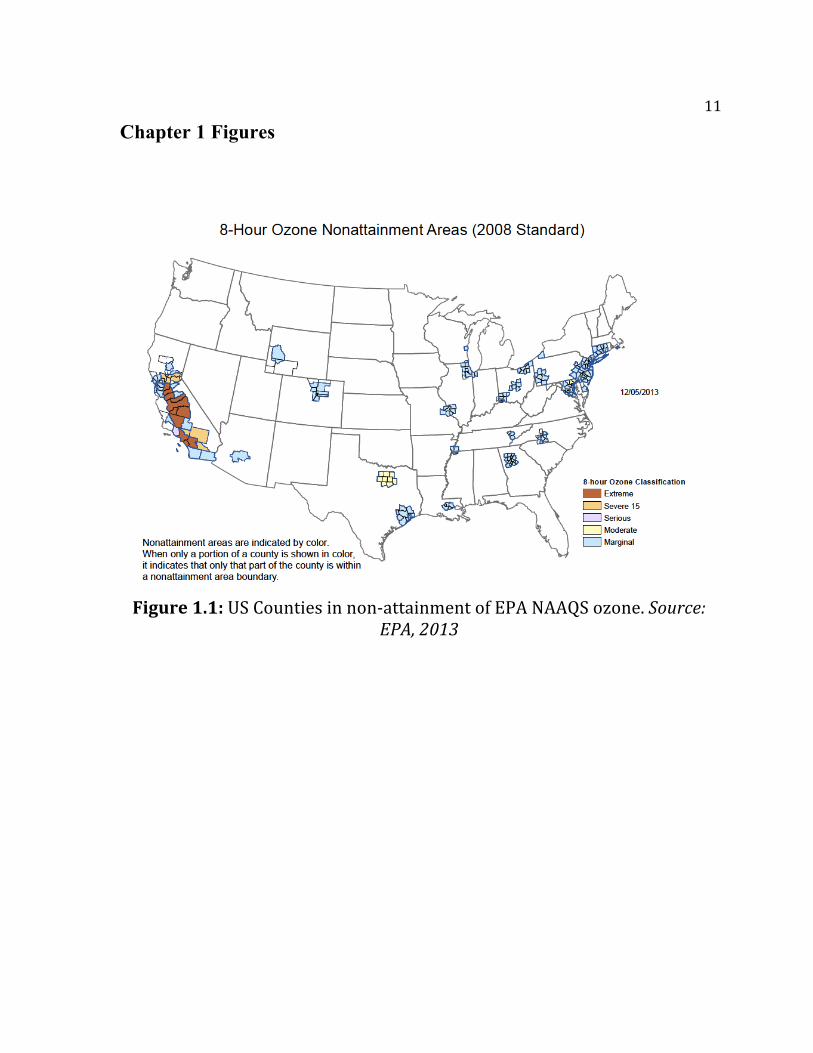
The National Ambient Air Quality Standards (NAAQS), established
under the Clean Air Act, set federal standards of allowable concentrations of
primary and secondary pollutants for counties in the United States. In the Front
Range, a number of counties are in marginal non-attainment of the NAAQS 8-
hour averaged ozone concentration (Figure 1.1). Ozone standards are both
primary and secondary so that they ensure the protection of both sensitive
groups and general human health. Non-attainment of O3 in the Front Range is
an ongoing motivation for continued air quality studies in the region including
both the DISCOVER-AQ and FRAPPE field campaigns.

!
!
8!Both primary and secondary pollutants are significant concerns as they
contribute to degradation of human health and loss of agricultural productivity.
Generally, air pollution by nature affects the respiratory systems of humans and
animals, but can also cause cardiac problems, cancer, and hematological
problems. Of the common pollutants in the Front Range, ozone and particulate
matter are harmful to agriculture causing reduced growth and death in plants
either directly or indirectly by changing the pH of the growing medium
(Seinfeld and Pandis, 2012).
Air pollutants observed in the Front Range come from a variety of
anthropogenic and biogenic sources (NEI, 2011). The common primary
pollutant, carbon monoxide, is a colorless and odorless gas produced when
incomplete combustion of organic substances occurs. Common sources of
carbon monoxide in the Front Range include motor vehicles and wildfires.
Nitrogen oxides, like carbon monoxide, form when nitrogen and oxygen
interact during combustion with sources including motor vehicles, industrial
sources, and biogenic sources like lightning and fertilizer (Figure 2.3).
Formaldehyde is a highly reactive gas at room temperature that is a byproduct
of volatile organic compounds oxidizing (Seinfeld and Pandis, 2012). Volatile
organic compounds are produced from natural sources such as forest fires and
!
!
9!from anthropogenic combustion processes in power plants and from fuel
combustion in vehicles.
One primary pollutant that is not found in a gaseous phase is particulate
matter. Particulate matter is not a single chemical molecule but rather a mixture
of varying particles of different sizes and compositions. It is categorized by
physical size with PM10 representing particles less than 10 microns in diameter
and PM2.5 representing particles less than 2.5 microns in diameter. PM10 is
commonly found emitting from fugitive sources like unpaved roads and heavy
construction areas, whereas PM2.5 can be found as a product of both biogenic
and anthropogenic combustion (Seinfeld and Pandis, 2012).
Secondary pollutants are not directly emitted from sources but rather
form in the atmosphere through chemical process such as photochemical
reactions (Jacob, 1999). These reactions occur when primary pollutants react
with each other and often with radiant energy like ultraviolet radiation. The
most common form of secondary pollution is photochemical smog that is made
up of volatile organic compounds, nitrogen oxides, and ozone. The large
majority of ozone found in the troposphere is not directly emitted but rather
forms when carbon monoxide, volatile organic compounds, and nitrogen oxides
react in the presence of ultraviolet light. Correspondingly, nitrogen dioxide

!
!
10!(NO2) is formed in the atmosphere when nitrogen oxide (NO) reacts with ozone
or other free radicals.
To gain insight into air pollution in the Front Range, Chapter 2 will
present the methods used to conduct a model to observational comparison of
July and August 2014 during the FRAPPE and DISCOVER-AQ Field
Campaigns. Chapter 3 will highlight general findings of the comparison, while
Chapter 4 will analyze a specific case study of high-observed ozone and model
performance. Finally, concluding remarks will be presented in Chapter 5.
!
!
11!Chapter 1 Figures
Figure'1.1:!US!Counties!in!non6attainment!of!EPA!NAAQS!ozone.!Source:(EPA,(2013

!
!
12!
0! 10000! 20000! 30000! 40000!
!Chemical!Manuf!!Non6ferrous!Metals!
!Pulp!&!Paper!!Ferrous!Metals!
!Mining!!Storage!and!Transfer!!Petroleum!ReMineries!
!NEC!!Cement!Manuf!
!Oil!&!Gas!Production!
Tons'of'NOx/year'
Industrial'Sources'
0.7!
26.11!
75!
200.89!
6129!
32909.53!
44939!
100107!
152703!
0! 40000! 80000! 120000! 160000!
Miscellaneous!Non6Industrial!
Bulk!Gasoline!Terminals!
Solvent!
Waste!Disposal!
Fires!
Biogenics!
Industrial!Processes!
Fuel!Combustion!
Mobile!
Tons'of'NOx/year'
NOx'Emissions'Sources'NEI'2011'@'Colorado'
Figure'1.2:!NEI!2011!NOx!inventory!for!Colorado!by!sector.!Source:(NEI(2011
Figure'1.3:'NEI!2011!NOx!inventory!for!Colorado!Industrial!Sources.!Source:(NEI(2011

!
!
13!Chapter 1 References
Baumann, K., Williams, E. J., Olson, J. a., Harder, J. W., & Fehsenfeld, F. C. (1997). Meteorological characteristics and spatial extent of upslope events during the 1993 Tropospheric OH Photochemistry Experiment. Journal of Geophysical Research, 102, 6199. doi:10.1029/96JD03251
Benedict, K. B., Day, D., Schwandner, F. M., Kreidenweis, S. M., Schichtel, B., Malm, W. C., & Collett, J. L. (2013). Observations of atmospheric reactive nitrogen species in Rocky Mountain National Park and across northern Colorado. Atmospheric Environment, 64, 66–76. doi:10.1016/j.atmosenv.2012.08.066
Bossert, J. E., & Cotton, W. R. (1994). Regional-Scale Flows in Mountainous Terrain. Part II: Simplified Numerical Experiments. Mon. Weather Rev. Retrieved from http://www.ncbi.nlm.nih.gov/entrez/query.fcgi?db=pubmed&cmd=Retrieve&dopt=AbstractPlus&list_uids=A1994NU46600005
Brown, S. S., Thornton, J. a., Keene, W. C., Pszenny, A. a P., Sive, B. C., Dubé, W. P., … Wolfe, D. E. (2013). Nitrogen, Aerosol Composition, and Halogens on a Tall Tower (NACHTT): Overview of a wintertime air chemistry field study in the front range urban corridor of Colorado. Journal of Geophysical Research: Atmospheres, 118, 8067–8085. doi:10.1002/jgrd.50537
Caiazzo, F., Ashok, A., Waitz, I. a., Yim, S. H. L., & Barrett, S. R. H. (2013). Air pollution and early deaths in the United States. Part I: Quantifying the impact of major sectors in 2005. Atmospheric Environment, 79, 198–208. doi:10.1016/j.atmosenv.2013.05.081
Christopherson, Robert W. (1992). Geosystems: An Introduction to Physical Geography. Macmillan Publishing Company. p. 155. ISBN 0-02-322443-6.
Dutton, S. J., Rajagopalan, B., Vedal, S., & Hannigan, M. P. (2010). Temporal patterns in daily measurements of inorganic and organic speciated PM2.5 in Denver. Atmospheric Environment, 44(7), 987–998. doi:10.1016/j.atmosenv.2009.06.006

!
!
14!EPA. (2013). 2011 National Emissions Inventory, Version 1 Technical Support
Document, (November).
Haagenson, P. (1979). Meteorological and climatological factors affecting Denver air quality. Atmospheric Environment (1967), 13(1977), 79–85. Retrieved from http://www.sciencedirect.com/science/article/pii/0004698179902476
Hansen, W. R., Chronic, J., & Matelock, J. (1978). Climatography of the Front Range Urban Corridor and vicinity, Colorado. A graphical summary of climatic conditions in a region of varied physiography and rapid urbanization.Professional Papers-US Geological Survey (USA).
Jacob, D. (1999). Introduction to atmospheric chemistry. Princeton University Press.
Montzka, A., Sweeney, C., Andrews, A., & Dlugokencky, M. (n.d.). Estimation of Emissions from Oil and Natural Gas Operations in Northeastern Colorado. Epa.Gov, 2010–2013. Retrieved from http://www.epa.gov/ttnchie1/conference/ei20/session6/gpetron.pdf
Neff, W. D. (1997). The Denver Brown Cloud Studies from the Perspective of Model Assessment Needs and the Role of Meteorology. Journal of the Air & Waste Management Association, 47(January 2015), 269–285. doi:10.1080/10473289.1997.10464447
Reddy, P. J. (1995). Development of a statistical model for forecasting episodes of visibility degradation in the Denver metropolitan area. Journal of Applied …, 34. Retrieved from http://journals.ametsoc.org/doi/abs/10.1175/1520-0450(1995)034%3C0616%3ADOASMF%3E2.0.CO%3B2
Regional Plan Association (2015). America 2015: Megaregions: The Front Range. http://www.america2050.org/front_range.html
Seinfeld, J. H., & Pandis, S. N. (2012). Atmospheric chemistry and physics: from air pollution to climate change. John Wiley & Sons.
!
!
15!Stohl, a., Spichtinger-Rakowsky, N., Bonasoni, P., Feldmann, H.,
Memmesheimer, M., Scheel, H. E., … Mandl, M. (2000). The influence of stratospheric intrusions on alpine ozone concentrations. Atmospheric Environment, 34(9), 1323–1354. doi:10.1016/S1352-2310(99)00320-9
Szoke, E. J. (1991). Eye of the Denver Cyclone. Monthly Weather Review. doi:10.1175/1520-0493(1991)119<1283:EOTDC>2.0.CO;2
Szoke, E. J., & Brady, R. H. (1989). Forecasting Implications of the 26 July 1985 Northeastern Colorado Tornadic Thunderstorm Case. Monthly Weather Review. doi:10.1175/15200493(1989)117<1834:FIOTJN>2.0.CO;2
Tripoli, G. J., & Cotton, W. R. (1989). Numerical Study of an observed Orogenic Mesoscale Convective Systems. Part I: Simulated Genesis and Comparison with Observations. Monthly Weather Review.
Val Martin, M., Heald, C. L., Lamarque, J.-F., Tilmes, S., Emmons, L. K., & Schichtel, B. A. (2015). How emissions, climate, and land use change will impact mid-century air quality over the United States: a focus on effects at national parks. Atmospheric Chemistry and Physics, 15(5), 2805–2823. doi:10.5194/acp-15-2805-2015
Wesley, D. A., & Pielke, R. A. (1990). Observations of blocking-induced convergence zones and effects on precipitation in complex terrain. Atmospheric Research. doi:10.1016/0169-8095(90)90014-4
Wilczak, J. M., & Glendening, J. W. (1988). Observations and mixed-layer modeling of a terrain-induced mesoscale gyre: The Denver cyclone. Monthly Weather Review, 116. Retrieved from http://journals.ametsoc.org/doi/abs/10.1175/1520-0493(1988)116%3C2688%3AOAMLMO%3E2.0.CO%3B2
Wolyn, P. G., & Mckee, T. B. (1994). The Mountain-Plains Circulation East of a 2-km-High North–South Barrier. Monthly Weather Review. doi:10.1175/1520-0493(1994)122<1490:TMPCEO>2.0.CO;2

!
!
16!Chapter 2: Methods !
The forecast model analyzed in this study was the research version of the
Rapid Refresh with Chemistry model (RR-Chem). The model is a rapid refresh
configuration of the Weather Research and Forecasting model coupled with
chemistry (WRF-Chem) run at NOAA/ESRL (Grell et al., 2005; Koch et al.,
2000). A number of observational data sets from ground observations, research
tower observatories, in situ aircraft observations, and satellite retrievals were
used to assess the RR-Chem model. Ground observations were obtained
through the AirNow air quality network and the Boulder Atmospheric
Observatory research facility. Aerial observations were included from the
DISCOVER-AQ field campaign using NASA’s P3B research aircraft along
with data from the FRAPPE field campaign obtained through NSF and NCAR’s
C-130 research aircraft. Satellite observations were obtained through NASA’s
Ozone Monitoring Instrument (OMI) aboard the Aura Satellite. Statistical
analysis was conducted using the aforementioned observational data sets to
assess model performance in the Front Range for the duration of the
DISCOVER-AQ and FRAPPE field campaigns.

!
!
17!RR-Chem Model Overview !
In this study, the RR-Chem model was used to forecast and quantify
meteorology and air chemistry. Meteorological model performance was
conducted on potential temperature, wind speed, and water vapor mixing ratio,
as they all are important in the governance of atmospheric chemistry (Jacob,
1999; Seinfeld and Pandis, 2012). The model’s chemical performance was
analyzed in terms of carbon monoxide, nitrogen dioxide, formaldehyde,
particulate matter, and ozone, as they are all predominate chemical species
found in the area and are detrimental to human health (EPA, 2012; Lave and
Seskin, 2013).
The RR-Chem model’s meteorology is generated through the Weather
Research and Forecasting model (WRF) (Grell et al., 2005). The WRF model is
a 3-dimensional numerical weather prediction and atmospheric simulation that
is a nonhydrostatic and compressible model (Grell et al., 2012; Skamarock et
al., 2008). The model is used by a variety of operational forecasting and
atmospheric research groups. The model resolution analyzed in this study has a
13.5 km by 13.5 km horizontal resolution and 51 vertical layers based on
hydrostatic pressure coordinates. Meteorological output used included
horizontal and vertical velocity components, perturbation potential temperature,
perturbation geopotential, and perturbation surface pressure of dry air. Model
!
!
18!output was generated every 3 hours with initialization occurring every 12 hours
at 00:00 UTC and 12:00 UTC.
Several WRF physics options were used in this model simulation. The
microphysics scheme used was the WRF single–moment 3–class and 5–class
schemes that have been found to improve the ice cloud-radiation feedback that
drives high-cloud physics, surface precipitation, and average temperature over
previous configurations (S.Y. Hong & Dudhia, 2004). The planetary boundary
layer (PBL) physics scheme used was the Yonsei University Scheme. This PBL
scheme has been found to improve vertical diffusion in the boundary layer with
more accurate prediction of convective inhibition (Hong et al., 2006). Cumulus
parameterization was based on Grell–Freitas Ensemble Scheme that is
commonly used in high-resolution mesoscale models not unlike the RR-Chem
model. This parameterization allows for interactions with aerosols simulating
more realistic precipitation and increases of water and ice in cloud tops (G.
Grell & Freitas, 2014). Longwave and shortwave radiation schemes were based
on RRTMG Shortwave and Longwave Schemes that have been found to
produce more accurate radiative forcing results when long lived greenhouse
gasses, ozone, and water vapor are included in the simulation (Iacono et al.,
2008).
!
!
19!The 2011 National Emissions Inventory (NEI) provided sectored
emissions sources for the RR-Chem model (EPA, 2013). Pollutants included in
the inventory are those that comprise the National Ambient Air Quality
Standards (NAAQS) in addition to Hazardous Air Pollutants (HAPs) detailed in
the Clean Air Act (Kuykendal, 2005). Emissions sources include point sources,
nonpoint sources, on-road sources, non-road sources, and event sources. Event
sources include significant anthropogenic and natural burning such as structure
fires and wildfires. Point sources relevant to the Front Range that have been
updated in the 2011 inventory to include industrial processes such as oil and gas
production (VOCs, CO, NOx), biomass burning (CO, VOCs), and agricultural
burning (PM2.5, SO2, CO, NOx, VOCs).
Biogenic emissions were provided through the Model of Emissions of
Gases and Aerosols from Nature (MEGAN) (Guenther et al., 2012). Lateral
boundary conditions for the model used 1-degree resolved conditions from the
Real-time Air Quality Modeling System (RAQMS) (Pierce, et al., 2007). The
RR-Chem model forecasts also included chemical deposition, photolysis, and
convective and turbulent chemical transport with the later calculated
concurrently with WRF (Fast et al., 2006).

!
!
20!The atmospheric chemical mechanism used in the model is based on
Version 2 of the Regional Acid Deposition Model (Chang et al., 1989;
Stockwell et al., 1990). The primary use of the Regional Acid Deposition
Model is for gas phase reactions in atmospheric chemistry models. Aerosol
parameterization, both primary and secondary, is based on the Modal Aerosol
Dynamics Model for Europe (Ackermann et al., 1998).
Observational Data !
Model validation of surface conditions was conducted using a number of
observational data sets including the AirNow air quality network and the
Boulder Atmospheric Observatory research facility. The AirNow air quality
network uses federal reference monitoring techniques in line with state
standards for air quality monitoring (Hawley, 2007). The network consists for
over 2,000 monitoring stations in over 300 cities that provide real time pollution
concentrations (Dye, AIRNow Program (U.S.), & Sonoma Technology Inc,
2003). Hourly data was used from monitoring stations throughout the Front
Range and the continental US (CONUS) to assess the accuracy of the model in
forecasting PM2.5 and O3 near-surface concentrations on an hourly basis.

!
!
21!The Boulder Atmospheric Observatory research facility, located in Erie,
Colorado, was used to analyze boundary layer conditions up to 300 meters
through use of the on-site tower (BAO Tower). Meteorological conditions in
addition to ozone concentrations at the ground, 100 m, 200 m, and 300 m were
used in model evaluation. BAO Tower was of particular interest in this study as
it was a tower site that was incorporated in the DISCOVER-AQ’s P3-B regular
flight plan. In supplement of BAO Tower, the Environmental Protection
Agency’s ceilometer and the University of Wisconsin – Madison’s High
Spectral Resolution (HSRL) LIDAR were used to monitor the planetary
boundary layer growth (Eloranta, 2005).
DISCOVER-AQ aircraft measurements were made using NASA’s P3-B
that had a maximum flight time of 14 hours and followed circuit pattern to
investigate temporal variation in atmospheric composition (Figure 2.1) (NASA,
2014). FRAPPE aircraft measurements were made using the NSF/NCAR C-130
that was able to fly for up to 10 hours with a 2,900-mile range (UCAR/NCAR -
Earth Observing Laboratory, 1994). The C-130’s flight plans were designed as
exploratory missions to investigate spatial variations in atmospheric
composition. Most all measurements from the C-130 were made within the
boundary layer. Airborne chemical measurements of CO, NO2, HCHO, O3, and
CH4 in addition to meteorological measurements of potential temperature,
!
!
22!humidity, and wind speed were used for model evaluation. Ozone and nitrogen
oxides were observed with a chemiluminescence instrument (Ray et al., 2009).
Formaldehyde was measured with an Aerolaser AL50, while carbon monoxide
was measured using a compact atmospheric multispecies spectrometer
(Bukowiecki, 2002; Li, Parchatka, Königstedt, & Fischer, 2012). Methane
observations were made using the Picarro instrument (Rella, 2010).
Satellite measurements of NO2 were made using the Ozone Measurement
Instrument (OMI) aboard the Aura Satellite (Ahmad et al., 2003). Satellite
overpasses occurred once daily in the early to mid afternoon when pollution
levels were typically highest. Measurements of NO2 were made of the total
tropospheric atmospheric nitrogen dioxide column value. To insure optimal
satellite data, no observations were included when the cloud fraction was above
30% and data quality flags were applied when interpolating and gridding
satellite retrievals to remove erroneous data. Satellite retrievals were taken with
a resolution of 13km x 24km at nadir and a 2600km swath width (Levelt et al.,
2006). Measurements were then interpolated and regridded to RR-Chem’s
13km x 13km horizontal spatial grid for statistical evaluation to the model.
!!!!

!
!
23!Chapter 2 Figures '
'
Figure'2.1:!NASA’s!P3B!flight!track!for!DISCOVER6AQ!2014.!!Source:(NASA,(2014(
((
!

!
!
24!Chapter 2 References !
Ackermann, I.J., Hass, H., Memmesheimer, M., Ebel, A., Binkowski, F.S., Shankar, U., 1998. Modal aerosol dynamics model for Europe: development and first applications. Atmospheric Environment 32 (17), 2981–2999.
Ahmad, S. P., Levelt, P. F., Bhartia, P. K., Hilsenrath, E., Leppelmeier, G. W., & Johnson, J. E. (2003). Atmospheric products from the ozone monitoring instrument (OMI). Society of Photo-Optical Instrumentation Engineers (SPIE) Conference Series, 5151(2), 619–630. doi:10.1117/12.506042
Bukowiecki, N., Dommen, J., Prevot, A. S. H., Richter, R., Weingartner, E., & Baltensperger, U. (2002). A mobile pollutant measurement laboratory—measuring gas phase and aerosol ambient concentrations with high spatial and temporal resolution. Atmospheric Environment, 36(36), 5569-5579.
Chang, J.S., Binkowski, F.S., Seaman, N.L., McHenry, J.N., Samson, P.J., Stockwell, W.R., Walcek, C.J., Madronich, S., Middleton, P.B., Pleim, J.E., Lansford, H.H., 1989. The regional acid deposition model and engineering model. State-of-Science/Technology, Report 4, National Acid Precipitation Assessment Program, Washington, DC.
Dye, T. S., AIRNow Program (U.S.), & Sonoma Technology Inc. (2003). Guidelines for Developing an Air Quality (ozone and PM2.5) Forecasting Program, 1.
Eloranta, E. E. (2005). High spectral resolution lidar (pp. 143-163). Springer New York.
EPA, (2013). 2011 National Emissions Inventory, Version 1 Technical Support Document, (November).
Fast, J. D., Gustafson, W. I., Easter, R. C., Zaveri, R. a., Barnard, J. C., Chapman, E. G., … Peckham, S. E. (2006). Evolution of ozone, particulates, and aerosol direct radiative forcing in the vicinity of Houston using a fully coupled meteorology-chemistry-aerosol model. Journal of Geophysical Research: Atmospheres, 111(21), 1–29. doi:10.1029/2005JD006721

!
!
25!Grell, G., McKeen, S., Barth, M., Pfister, G., Wiedinmyer, C., Fast, J. D., ... &
Freitas, S. (2012). WRF/Chem Version 3.3 User's Guide. US Department of Commerce, National Oceanic and Atmospheric Administration, Oceanic and Atmospheric Research Laboratories, Global Systems Division.
Grell, G. a., Peckham, S. E., Schmitz, R., McKeen, S. a., Frost, G., Skamarock, W. C., & Eder, B. (2005). Fully coupled “online” chemistry within the WRF model. Atmospheric Environment, 39(37), 6957–6975. doi:10.1016/j.atmosenv.2005.04.027
Grell, G., & Freitas, S. R. (2014). A scale and aerosol aware stochastic convective parameterization for weather and air quality modeling. Atmospheric Chemistry and Physics, 14(10), 5233–5250. doi:10.5194/acp-14-5233-2014
Guenther, a. B., Jiang, X., Heald, C. L., Sakulyanontvittaya, T., Duhl, T., Emmons, L. K., & Wang, X. (2012). The model of emissions of gases and aerosols from nature version 2.1 (MEGAN2.1): An extended and updated framework for modeling biogenic emissions. Geoscientific Model Development, 5(6), 1471–1492. doi:10.5194/gmd-5-1471-2012
Hawley, K. (2007). Federal Register, 72(53), 81–95.
Hong, S. Y., & Dudhia, J. (2004). Testing of a new nonlocal boundary layer vertical diffusion scheme in numerical weather prediction applications. Bulletin of the American Meteorological Society, 2(1), 2213–2218.
Hong, S.-Y., Noh, Y., & Dudhia, J. (2006). A New Vertical Diffusion Package with an Explicit Treatment of Entrainment Processes. Monthly Weather Review, 134(9), 2318–2341. doi:10.1175/MWR3199.1
Iacono, M. J., Delamere, J. S., Mlawer, E. J., Shephard, M. W., Clough, S. a., & Collins, W. D. (2008). Radiative forcing by long-lived greenhouse gases: Calculations with the AER radiative transfer models. Journal of Geophysical Research: Atmospheres, 113(13), 1–8. doi:10.1029/2008JD009944
Jacob, D. (1999). Introduction to atmospheric chemistry. Princeton University Press.

!
!
26!Koch, S. E., Benjamin, S. G., Mcginley, J. a, Brown, J. M., Schultz, P., Szoke,
E. J., … Grell, G. (2000). Real-Time Applications of the Wrf Model At the Forecast Systems Laboratory, 1–6.
Kuykendal, W. (2005). Emissions inventory guidance for implementation of ozone and particulate matter national ambient air quality standards (NAAQS) and regional haze regulations. DIANE Publishing.
Lave, L. B., & Seskin, E. P. (2013). Air pollution and human health. Routledge.
Levelt, P. F., Hilsenrath, E., Leppelmeier, G. W., Van Den Oord, G. H. J., Bhartia, P. K., Tamminen, J., … Veefkind, J. P. (2006). Science objectives of the ozone monitoring instrument. IEEE Transactions on Geoscience and Remote Sensing, 44(5), 1199–1207. doi:10.1109/TGRS.2006.872336
Li, J., Parchatka, U., Königstedt, R., & Fischer, H. (2012). Real-time measurements of atmospheric CO using a continuous-wave room temperature quantum cascade laser based spectrometer. Optics Express, 20(7), 7590. doi:10.1364/OE.20.007590
NASA, (2014). NASA P-3B Airborne Science Laboratory. http://www.nasa.gov/pdf/541828main_P-3BFactSheet.pdf
Pierce, R. B., et al. 2007: Chemical data assimilation estimates of continental U.S. ozone and nitrogen budgets during the Intercontinental Chemical Transport Experiment–North America, J. Geophys. Res., 112, D12S21, doi:10.1029/2006JD007722.Ray, J. D., Stedman, D. H., & Wendel, G. J. (1986). Fast chemiluminescent method for measurement of ambient ozone. Analytical Chemistry, 58(3), 598-600.
Rella, C. (2010). Accurate Greenhouse Gas Measurements in Humid Gas Streams Using the Picarro G1301 Carbon Dioxide / Methane / Water Vapor Gas Analyzer Experimental Determination of the Water Vapor Correction for the G1301. Water.
Seinfeld, J. H., & Pandis, S. N. (2012). Atmospheric chemistry and physics: from air pollution to climate change. John Wiley & Sons.

!
!
27!Skamarock, W. C., Klemp, J. B., Dudhi, J., Gill, D. O., Barker, D. M., Duda,
M. G., … Powers, J. G. (2008). A Description of the Advanced Research WRF Version 3. Technical Report, (June), 113. doi:10.5065/D6DZ069T
Stockwell, W.R., Middleton, P., Chang, J.S., Tang, X., 1990. The second-generation regional acid deposition model chemical mechanism for regional air quality modeling. Journal of Geophysical Research 95, 16343–16367.
UCAR/NCAR - Earth Observing Laboratory, (1994). NSF/NCAR Hercules C130 Aircraft. http://dx.doi.org/10.5065/D6WM1BG0

!
!
28!Chapter 3: Model Evaluation
Introduction
Model evaluation is an important process in determining the strengths
and deficiencies of chemical forecasting simulations that give key insights to air
quality policy questions. Due to the complicated nature of atmospheric
chemical modeling, meteorological and chemical evaluations are both needed
due to the interdependent nature of meteorology and air chemistry. Ideally, each
model grid box would be analyzed continuously but due to limited resources, a
mixture of ground observations, aircraft in situ measurements, and satellite
observations are used to holistically assess the model. Ground observations
monitor near surface atmospheric conditions, while aircraft and satellite
observations deliver observations of the vertical distribution and column
concentrations of atmospheric pollutants.
Ground stations provide near surface pollution measurements that help
scientists understand the impact of air pollution on populations and crops.
Aircraft measurements allow one to gain a vertically resolved understanding of
how well the model performs throughout the troposphere. While ground
stations and aircraft measurements are convenient, they are often spatially
limited, so satellite measurements allow for more all-inclusive spatial
!
!
29!assessment. Like ground and aircraft observations, satellite comparisons also
come with negative tradeoffs. Ambiguity in air mass weighting factors can blur
the truth of satellite retrievals, and lack of vertical resolution hampers model
assessment at otherwise discretized levels throughout the atmosphere.
In the comparison, we utilize the AirNow network both in the CONUS in
addition to the network in Colorado. Aircraft measurements from both NASA’s
P3B and NCAR’s C130 allow for vertically resolved meteorological and
chemical assessment of the model. Finally, NASA’s ozone monitoring unit
aboard the Aura Satellite is used to observe column nitrogen dioxide levels for
CONUS and Colorado.
Ground Observation Comparison
Model to ground-level chemical analysis was performed with a series
statistical metrics and observational data sets. The AirNow Network provided
hourly ozone (O3) and particulate matter (PM2.5) measurements that were
compared with model output at the same locations (Dye et al., 2003). AirNow
sites are more often located near urban environments so assessment is more
indicative of modeling accuracy, or lack thereof, of populated regions (Figure
3.1; Figure 3.2). For our evaluation, the majority of AirNow sites were located
!
!
30!in and around the Denver Metropolitan Area, home of the DISCOVER-AQ and
FRAPPE Field Campaigns.
Continental United States AirNow Results
Ground level ozone in CONUS was in general agreement with model
simulations with a correlation of 0.65, a bias of -8.69 ppb, and a root mean
square error of 16.21 ppb when concentrations under 120 ppb were analyzed
(Figure 3.5). Concentrations of ozone above 120 ppb were not used in statistical
analysis due to the likelihood of observational errors. Similarly, PM2.5
measurements under 100 µg/m3 were analyzed across CONUS with a lower
correlation than ozone, 0.39 (Figure 3.3). Despite a lower correlation between
model and observations, the mean bias of -2.34 µg/m3, and the root mean
square error of 9.4 µg/m3 were smaller than what was found for ozone.
Colorado AirNow Results !
For the interior of Colorado, ozone was modeled with a correlation of
0.66, similar to CONUS (Figure 3.6). Model bias was substantially improved
relative to the overall performance in the CONUS domain with a mean bias of -
0.21 ppb and a root mean squared error of 12.82 ppb. Particulate matter less
!
!
31!than 2.5 microns in Colorado held the weakest correlation of 0.19 (Figure 3.4).
However, mean bias and root mean squared error for PM2.5 were improved
compared to CONUS with values of -0.71 µg/m3 and 5.7 µg/m3 respectively.
AirNow Discussion !
In terms of ozone, model accuracy was similar to past studies using
WRF-Chem at a model resolution of 12 km that found correlations in the range
of 0.6 to 0.7 but generally better than other atmospheric chemistry models
(McKeen et al., 2007; Simon, Baker, & Phillips, 2012; Žabkar et al., 2015).
Despite the promising findings, it is important to question if the model’s
performance for a secondary pollutant like ozone is correct for the right reasons
or the wrong reasons. Due to the nonlinear relation between volatile organic
compounds and nitrogen oxides, the primary ingredients of tropospheric ozone,
overestimation of nitrogen oxides can lower ozone significantly in certain
regimes (Jacob, 1999).
PM2.5 performed with a slightly less degree of accuracy compared with
previous studies (McKeen et al., 2007; Saide et al., 2011; Simon et al., 2012).
Variations in past studies’ gas phase mechanism and configuration result in
varying modeling results of particulate matter (Zhang, Chen, Sarwar, & Schere,

!
!
32!2012). Greater exploration into other chemical mechanisms may be a viable
path for improvement of PM2.5 in the RR-Chem simulation. In addition,
variations in particulate matter emissions compounded by the complex terrain
have proven to be difficult to model and aerosols during the field campaigns
were lower than what is generally expected in the Front Range (Saide et al.,
2011).
Aircraft in situ Comparison !
NASA’s P3B and NCAR’s C130 were utilized in our model assessment
to vertically resolve the atmosphere for chemical and meteorological variables.
In terms of meteorology, potential temperature, wind speed, and water vapor
mixing ratio were used to assess the model’s atmospheric stability and
horizontal and vertical mixing. Chemically, ozone, methane, carbon monoxide,
formaldehyde, and nitrogen dioxide were analyzed to gain a greater
understanding for some of the more predominate air pollutants in the Front
Range (EPA, 2013). Flights for the P3B and C130 were made nearly everyday,
sometimes twice daily, for the entirety of the field campaigns. In addition to
vertically discretized measurements, median column amounts were also
calculated for the five chemical species.

!
!
33!Potential Temperature !
Potential temperature, a common measure of atmospheric static stability,
was measured throughout the atmosphere by both the P3B and C130 (Figure
3.7; Figure 3.8). Generally, the RR-Chem model accurately predicted potential
temperature below 500mb. Above 500mb, there was slight underprediction but
varying sample size limited the number of observations in that pressure regime.
C130 observations showed an inversion commonly occurring below 800mb that
the model did not predict. This discrepancy could indicate an improperly
modeled boundary layer or near surface inversions. If an inversion is not
accounted for in the model, pollutant concentrations may be underestimated due
to greater vertical mixing as inversions typically limit mixing height thus
increasing near surface concentrations (Marshall and Plumb, 1965).
Wind Speed !
The horizontal mixing of pollutants and the subsequent concentration of
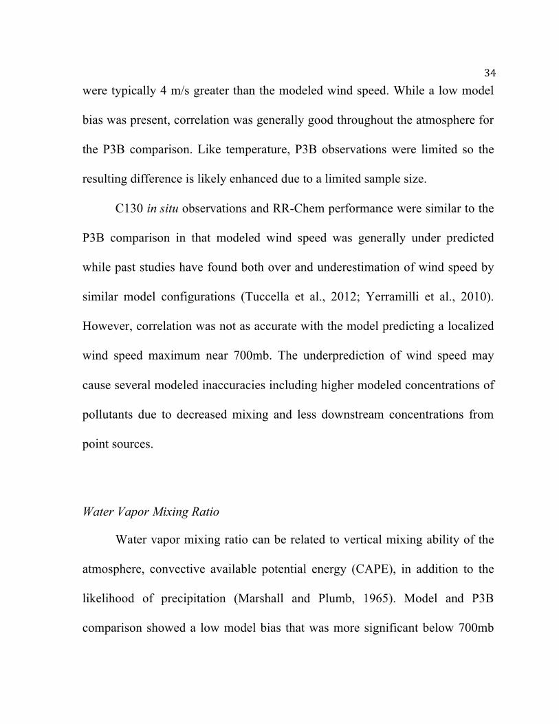
pollutants is primarily controlled by the wind, highlighting the importance in
the accurate modeling of wind speed and direction (Ying, Tie, & Li, 2009). For
both in situ observational datasets, modeled wind speed was underpredicted
throughout the entire atmosphere (Figure 3.9; Figure 3.10). P3B observations
!
!
34!were typically 4 m/s greater than the modeled wind speed. While a low model
bias was present, correlation was generally good throughout the atmosphere for
the P3B comparison. Like temperature, P3B observations were limited so the
resulting difference is likely enhanced due to a limited sample size.
C130 in situ observations and RR-Chem performance were similar to the
P3B comparison in that modeled wind speed was generally under predicted
while past studies have found both over and underestimation of wind speed by
similar model configurations (Tuccella et al., 2012; Yerramilli et al., 2010).
However, correlation was not as accurate with the model predicting a localized
wind speed maximum near 700mb. The underprediction of wind speed may
cause several modeled inaccuracies including higher modeled concentrations of
pollutants due to decreased mixing and less downstream concentrations from
point sources.
Water Vapor Mixing Ratio ! Water vapor mixing ratio can be related to vertical mixing ability of the
atmosphere, convective available potential energy (CAPE), in addition to the
likelihood of precipitation (Marshall and Plumb, 1965). Model and P3B
comparison showed a low model bias that was more significant below 700mb

!
!
35!(Figure 3.11). The model, on average, underpredicted the mixing ratio by
approximately 1g/kg below the 700mb pressure level whereas above, the model
underprediction was less significant with only an average difference of a few
tenths of a gram per kilogram. Similar to other the meteorological observations,
lacks of measurements above 500mb were likely to blame for the statistical
variations at these altitudes.
C130 and model comparison was similar to the P3B below 700mb with
model underprediction of water vapor while above the 700mb level, the model
slightly overpredicted water vapor, in contrast to the consistent under prediction
by the model with regard to the P3B flight track (Figure 3.12). Similar
underprediction of water vapor and relative humidity has previously been
documented (Fast et al., 2006; Yerramilli et al., 2010). Underprediction by the
model for both in situ datasets would most likely result in the model to
underestimate convection and precipitation and thus less vertical mixing and
wet deposition in the chemical predictions.
Ozone !
Ozone was generally well predicted for both the P3B and C130 modeled
flight track (Figure 3.13; Figure 3.14). P3B in situ measurements below 700mb

!
!
36!showed a slightly low model bias but were still well correlated. Above 700mb,
the RR-Chem model showed no significant bias when compared to in situ P3B
measurements. The average P3B column measurement was approximately
30•1015 mol/cm2, 1.1 DU, greater than the RR-Chem model with the median
situ column amount of 584•1015 mol/cm2, 21.7 DU, and a modeled column
amount of 552•1015 mol/cm2, 20.5 DU.
C130 in situ measurements were slightly less correlated with a greater
overall bias compared to the model. While little model bias occurred below
800mb, slight overprediction of approximately 10ppbv ozone arose between
750mb and 550mb. In contrast from the P3B observations and model track, RR-
Chem had a slightly higher median column amount of 573•1015 mol/cm2, 21.3
DU, compared to the median in situ column of 549•1015 mol/cm2, 20.4 DU.
While either aircraft observed little model bias, ozone is not directly emitted
into the atmosphere. Instead, ozone concentrations are governed by precursors
like volatile organic compounds, nitrogen oxides, and carbon monoxide, in
addition to atmospheric conditions. Like the findings for the AirNow analysis,
further investigation into those factors is needed to determine if ozone
production is accurate due to correct emissions estimates and model physics or
due to incorrect modeling (Georg a. Grell et al., 2005; Yerramilli et al., 2010).

!
!
37!Methane !
In addition to ozone and its precursors, methane emissions in the Front
Range are an ongoing problem. For the in situ analysis of methane, an
adjustment was applied to background methane levels since the RAQMS
boundary conditions were fixed at 1990 levels (EPA, 2013). In the upper
troposphere above 700mb, both the C130 and P3B accurately captured methane
(Figure 3.15; Figure 3.16). Both airplanes observed significant enhancement of
methane below 700mb that the model failed to capture. The P3B observed the
highest methane measurements between the two aircraft with readings as high
as 2800 ppbv, well above the model peak predictions at the same pressure level
of approximately 1850 ppbv. Closest to the surface, in situ observations, even at
their lowest measurements, were still higher than model prediction.
The model’s low bias may be attributed to decision not to use
anthropogenic emissions in this particular configuration of RR-Chem. Despite
this, median column amounts for both aircraft when averaged throughout the
entire atmosphere were satisfactory with the P3B and RR-Chem median column
amounts of 17.3•1018 mol/cm2 and 17.2•1018 mol/cm2, respectively. Similarly,
the C130, that observed less variation of methane compared to the model near
the surface, had a median column measurement of 17.4•1018 mol/cm2 compared
to the model’s column measurement of 17.4•1018 mol/cm2.

!
!
38!The closer agreement between the C130 and model track could possibly
be attributed to the aircraft flying over more rural and mountainous areas where
anthropogenic emissions are not as common. The greater variation in methane
in the upper troposphere observed by the C130 compared to the P3B could also
be explained through upslope flow carrying methane into the more mountainous
regions where the C130 flew. It is difficult to compare methane to previous
studies without the inclusion of point sources, as it should be a priority to
include those inventories in updates to the model.
Carbon Monoxide !
Carbon monoxide, typically a pollutant resulting from combustion within
automobiles, was modeled and observed throughout the Front Range with
relatively good accuracy (Figure 3.17; Figure 3.18). The P3B and RR-Chem
model mapped to the P3B flight track observed a relative peak in carbon
monoxide around 800mb with higher concentrations being observed generally
closer to the surface. Less model variance and the most accurate model results
came above 600mb. Nearest to the surface, significant spikes in carbon
monoxide concentrations were observed that were not captured by RR-Chem.
Overall, the model over predicted the median column amount by approximately

!
!
39!90•1015 mol/cm2 with the model predicting 993•1015 mol/cm2 and the P3B in
situ instrument observing 905•1015 mol/cm2.
While the median column difference between C130 in situ measurements
and the modeled flight track was smaller with column amounts of 934•1015
mol/cm2 and 964•1015 mol/cm2 respectively, the model did not capture
significant surface enhancement that was observed. While the model was
unable to capture near surface enhancement, it performed well compared to
previous studies evaluating carbon monoxide (Tie et al., 2007).
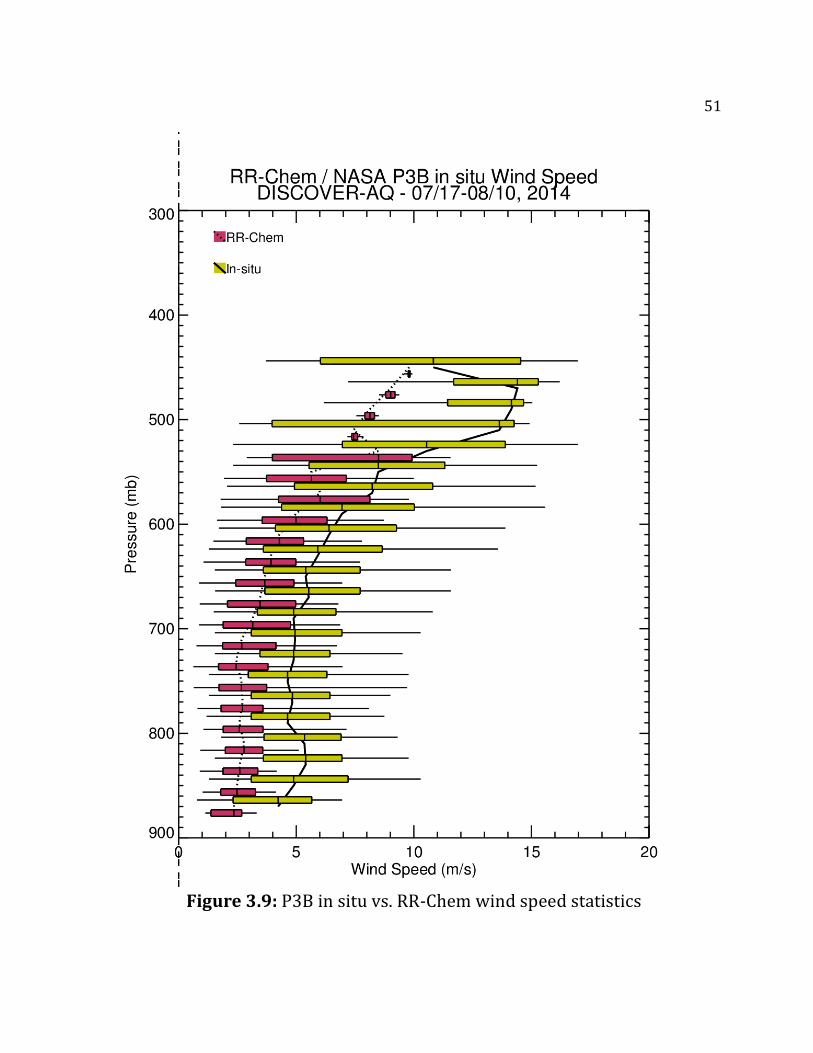
Formaldehyde ! Formaldehyde, a common tracer of volatile organic compounds was also
observed by both the P3B and C130 (Figure 3.19; Figure 3.20). Unlike
methane, near surface enhancement of HCHO was over predicted by the model.
In both in situ observational datasets, a peak in HCHO occurs near 800mb to
850mb with lower observations near the surface. Generally above 800mb,
HCHO in-situ was well correlated with the RR-Chem model. The P3B flight
track in particular had the greatest difference to the model near the surface with
a median RR-Chem column of 10.5•1015 mol/cm2 compared with an in situ
measurement of 8.4•1015 mol/cm2. The C130 median column was 9.7•1015

!
!
40!mol/cm2 compared with an RR-Chem median column value of 10.1•1015
mol/cm2. This is in contrast to previous studies that have found an
underestimation of HCHO using WRF-Chem and CMAQ and is most likely an
issue with the NEI 2011 emissions inventory (Barth et al., 2014; Czader, Li, &
Rappenglueck, 2013).
Nitrogen Dioxide !
Nitrogen dioxide measurements aboard both aircrafts found substantial
overestimation by the model through most of the troposphere (Figure 3.21;
Figure 3.22). P3B observations show the most significant overestimation of
NO2 is found below 600mb where RR-Chem over predicted concentrations by
approximately 2-3 times the amount observed. Above 600mb, the P3b show
most consistent but varying observations when compared to the model. The
model median column was about 3 times higher than the in situ observations
with respective column amounts of 8.4•1015 mol/cm2 and 3.0•1015 mol/cm2.
C130 in situ measurements also pointed towards a high bias by the model
from approximately 550mb to the surface. Above 550mb unexplained high
measurements were reported by the C130, well above model results. The origin
of these anomalously high measurements remains unresolved. Due to the high

!
!
41!measurements, the in situ median column value is greater than the model with a
value of 9.5•1015 mol/cm2 compared to the RR-Chem model’s median column
value of 6.3•1015 mol/cm2. Despite the high-observed values by the C130,
modeled NO2 is overestimated by the model below 600mb.
Several recent studies have also found modeled overestimations of NOx
and have pointed at incorrect mobile emissions as a possible source of the error
(Anderson et al., 2014; Ghude et al., 2013; Valin, Russell, Hudman, & Cohen,
2011). Nonlinear dependence of nitrogen oxides, VOCs, and ozone production
imply that since NO2 is incorrect, ozone concentrations that were being
modeled with generally good agreement to observations may in fact be
correctly modeled for the wrong reasons in urban environments. To further
evaluate RR-Chem’s NO2 modeling, we employ NASA’s ozone monitoring
instrument to evaluate tropospheric nitrogen dioxide column values.
Aura Satellite Comparison
The Ozone Monitoring Instrument (OMI) aboard NASA’s Aura satellite
was used to calculate the NO2 column over Colorado and the continental United
States (Figure 3.23). Model output for NO2, generated every 3 hours, was used
at 21 UTC since that generally aligned with the average OMI overpass time for
Colorado that most often occurred between 19 and 23 UTC. RR-Chem NO2 was

!
!
42!vertically integrated for the troposphere and binned to the model’s 13.5km
horizontal resolution using the nearest neighbor algorithm. The top of the
troposphere was calculated based on the World Meteorological Organizations
standard for lapse rate in the tropopause, 2K/km (McCalla, 1981). Based on
observations made by the satellite, areas where the cloud radiance fraction was
greater than 30% were not included in statistical calculations of model
performance of NO2 tropospheric column.
Colorado OMI Comparison !
OMI observations of Colorado and the Front Range show a regional
maximum of approximately 4•1015 mol/cm2 centered on the Denver
metropolitan area. Due to the persistence of clouds over the Rocky Mountains,
a significant area could not be calculated due to cloud contamination. RR-Chem
modeled NO2 column values were spatially similar with a regional maximum
over the Denver metropolitan area, but the model was nearly 3 times higher
than observed values at 10•1015 mol/cm2. Beyond urban areas, background
nitrogen dioxide column values are more closely aligned to modeled
concentrations. Statistically, the correlation between model and observations is
0.38 with a high model bias of 0.69•1015 mol/cm2 and a root mean squared error

!
!
43!of 1.89•1015 mol/cm2 (Figure 3.24). Typically, the model shows a high bias at
observational maxima and minima.
Continental United States OMI Comparison !
Observations of the Ozone Monitoring Instrument were also compared to
modeled values for the continental United States. Like Colorado, modeled NO2
over the United States was greater than observed column values over most
metropolitan areas. The most significant overestimation was observed in the
Western United States, especially in the major cities of California like Los
Angeles, San Francisco, and Sacramento. In rural areas, there was good
agreement, relative to urban areas, with slight underestimation in very rural
areas. Model to observation correlation for the continental United States was
just under what was calculated for Colorado with a correlation coefficient of
0.35 and high model bias of 0.52•1015 mol/cm2 and root mean squared error of
2.10•1015 mol/cm2 (Figure 3.23). Like Colorado, the model simulated a high
bias compared to the observational dataset. Beyond the continental United
States, the RR-Chem model also significantly overpredicted NO2 around the
Calgary, Canada metropolitan area and surrounding regions.
!

!
!
44!OMI Discussion !
Similar to the in situ findings, nitrogen dioxide is overestimated by
approximately the same amount throughout not only Colorado but also the
United States. Similar findings, while not to the extent of ours, have found
problems with the emissions inventories and modeling of nitrogen oxides
(Anderson et al., 2014; Ghude et al., 2013; Valin et al., 2011). One major
difference is that this study only used tropospheric column amounts without
applying an air mass factor, potentially biasing results.
Model Performance Discussion !! The evaluation of the modeling of meteorology and chemistry by the RR-
Chem model presented a mix bag of strengths and weaknesses of the model.
Potential temperature was a relatively strong suit of the model with very little
difference between simulation and aircraft observations. Chemically, ozone and
carbon monoxide also performed well in model to observation analysis.
Similarly, background methane concentrations performed well but
anthropogenic enhancement near the surface was not included in this model
simulation so it was not captured. Water vapor mixing ratio was slightly
underpredicted by the model, which possibly contributed to problems in

!
!
45!capturing convection and mixing in the atmosphere. Formaldehyde and nitrogen
dioxide were both overestimated by the model with overestimation of
formaldehyde occurring near surface and nitrogen dioxide throughout the entire
tropospheric column. These are likely problems not with the RR-Chem model
itself but instead with the NEI 2011 emissions inventory.

!
!
46!Chapter 3 Figures
Figure'3.1:'AirNow!Network!with!modeled!RR6Chem!PM2.5!July!28th,!2014
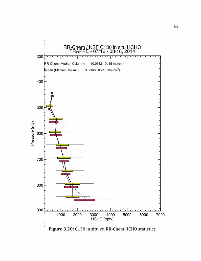
Figure'3.2:'AirNow!Network!with!modeled!RR6Chem!O3!July!28th,!2014

!
!
47!
Figure'3.3:'AirNow!Network!vs.!RR6Chem!PM2.5!statistics!in!the!United!States
Figure'3.4:'AirNow!Network!vs.!RR6Chem!PM2.5!statistics!in!Colorado

!
!
48!
Figure'3.5:'AirNow!Network!vs.!RR6Chem!O3!statistics!in!the!United!States
Figure'3.6:'AirNow!Network!vs.!RR6Chem!O3!statistics!in!Colorado

!
!
49!
Figure'3.7:'P3B!in!situ!vs.!RR6Chem!potential!temperature!statistics

!
!
50!
Figure'3.8:'C130!in!situ!vs.!RR6Chem!potential!temperature!statistics
!
!
51!
Figure'3.9:'P3B!in!situ!vs.!RR6Chem!wind!speed!statistics

!
!
52!
Figure'3.10:'C130!in!situ!vs.!RR6Chem!wind!speed!statistics

!
!
53!
Figure'3.11:'P3B!in!situ!vs.!RR6Chem!potential!water!vapor!mixing!ratio!statistics

!
!
54!
Figure'3.12:'C130!in!situ!vs.!RR6Chem!potential!water!vapor!mixing!ratio!statistics

!
!
55!
Figure'3.13:'P3B!in!situ!vs.!RR6Chem!O3!statistics

!
!
56!
Figure'3.14:'C130!in!situ!vs.!RR6Chem!O3!statistics

!
!
57!
Figure'3.15:'P3B!in!situ!vs.!RR6Chem!CH4!statistics

!
!
58!
Figure'3.16:'C130!in!situ!vs.!RR6Chem!CH4!statistics

!
!
59!
Figure'3.17:'P3B!in!situ!vs.!RR6Chem!CO!statistics

!
!
60!
Figure'3.18:'C130!in!situ!vs.!RR6Chem!CO!statistics

!
!
61!
Figure'3.19:'P3B!in!situ!vs.!RR6Chem!HCHO!statistics
!
!
62!
Figure'3.20:'C130!in!situ!vs.!RR6Chem!HCHO!statistics

!
!
63!
Figure'3.21:'P3B!in!situ!vs.!RR6Chem!NO2!statistics

!
!
64!
Figure'3.22:'C130!in!situ!vs.!RR6Chem!NO2!statistics

!
!
65!
Figure'3.23:'OMI!tropospheric!NO2!satellite!on!July!28th,!2014.!Source:(NASA,(2014
Figure'3.24:'OMI!vs.!RR6Chem!tropospheric!NO2!statistics!for!CONUS

!
!
66!
Figure'3.24:'OMI!vs.!RR6Chem!tropospheric!NO2!statistics!for!Colorado

!
!
67!Chapter 3 References
Anderson, D. C., Loughner, C. P., Diskin, G., Weinheimer, A., Canty, T. P., Salawitch, R. J., … Dickerson, R. R. (2014). Measured and modeled CO and NOy in DISCOVER-AQ: An evaluation of emissions and chemistry over the eastern US. Atmospheric Environment, 96, 78–87. doi:10.1016/j.atmosenv.2014.07.004
Barth, M. C., Wong, J., Bela, M. M., Pickering, K. E., Li, Y., & Cummings, K. (2014). Simulations of L ightning - Generated NOx for Parameterized C onvection in the WRF - Chem model, 4(2), 15–20.
Czader, B. H., Li, X., & Rappenglueck, B. (2013). CMAQ modeling and analysis of radicals, radical precursors, and chemical transformations. Journal of Geophysical Research: Atmospheres, 118(19), 11376–11387. doi:10.1002/jgrd.50807
Dye, T. S., AIRNow Program (U.S.), & Sonoma Technology Inc. (2003). Guidelines for Developing an Air Quality (ozone and PM2.5) Forecasting Program, 1.
EPA, U. (2013). 2011 National Emissions Inventory, Version 1 Technical Support Document, (November).
Fast, J. D., Gustafson, W. I., Easter, R. C., Zaveri, R. a., Barnard, J. C., Chapman, E. G., … Peckham, S. E. (2006). Evolution of ozone, particulates, and aerosol direct radiative forcing in the vicinity of Houston using a fully coupled meteorology-chemistry-aerosol model. Journal of Geophysical Research: Atmospheres, 111(21), 1–29. doi:10.1029/2005JD006721
Ghude, S. D., Pfister, G. G., Jena, C., Van Der A, R. J., Emmons, L. K., & Kumar, R. (2013). Satellite constraints of nitrogen oxide (NOx) emissions from India based on OMI observations and WRF-Chem simulations. Geophysical Research Letters, 40(2), 423–428. doi:10.1029/2012GL053926

!
!
68!Grell, G. a., Peckham, S. E., Schmitz, R., McKeen, S. a., Frost, G., Skamarock,
W. C., & Eder, B. (2005). Fully coupled “online” chemistry within the WRF model. Atmospheric Environment, 39(37), 6957–6975. doi:10.1016/j.atmosenv.2005.04.027
Jacob, D. (1999). Introduction to atmospheric chemistry. Princeton University Press.
Marshall, J., & Plumb, R. A. (1965). Atmosphere, ocean and climate dynamics: an introductory text (Vol. 8). Academic Press.
McCalla, C. (1981). Objective Determination of the Tropopause Using WMO Operational Definitions. US Department of Commerce, National Oceanic and Atmospheric Administration, National Weather Service, National Meteorological Center.
McKeen, S. a., Chung, S. H., Wilczak, J., Grell, G., Djalalova, I., Peckham, S., … Yu, S. (2007). Evaluation of several PM2.5 forecast models using data collected during the ICARTT/NEAQS 2004 field study. Journal of Geophysical Research: Atmospheres, 112(10), 1–20. doi:10.1029/2006JD007608
Saide, P. E., Carmichael, G. R., Spak, S. N., Gallardo, L., Osses, A. E., Mena-Carrasco, M. a., & Pagowski, M. (2011). Forecasting urban PM10 and PM2.5 pollution episodes in very stable nocturnal conditions and complex terrain using WRF-Chem CO tracer model. Atmospheric Environment, 45(16), 2769–2780. doi:10.1016/j.atmosenv.2011.02.001
Simon, H., Baker, K. R., & Phillips, S. (2012). Compilation and interpretation of photochemical model performance statistics published between 2006 and 2012. Atmospheric Environment, 61, 124–139. doi:10.1016/j.atmosenv.2012.07.012
Tie, X., Madronich, S., Li, G., Ying, Z., Zhang, R., Garcia, A. R., … Liu, Y. (2007). Characterizations of chemical oxidants in Mexico City: A regional chemical dynamical model (WRF-Chem) study. Atmospheric Environment, 41(9), 1989–2008. doi:10.1016/j.atmosenv.2006.10.053

!
!
69!Tuccella, P., Curci, G., Visconti, G., Bessagnet, B., Menut, L., & Park, R. J.
(2012). Modeling of gas and aerosol with WRF/Chem over Europe: Evaluation and sensitivity study. Journal of Geophysical Research: Atmospheres, 117(3), 1–15. doi:10.1029/2011JD016302
Valin, L. C., Russell, a. R., Hudman, R. C., & Cohen, R. C. (2011). Effects of model resolution on the interpretation of satellite NO2 observations. Atmospheric Chemistry and Physics, 11(22), 11647–11655. doi:10.5194/acp-11-11647-2011
Yerramilli, A., Challa, V. S., Dodla, V. B. R., Dasari, H. P., Young, J. H., Patrick, C., … Swanier, S. J. (2010). Simulation of Surface Ozone Pollution in the Central Gulf Coast Region Using WRF/Chem Model: Sensitivity to PBL and Land Surface Physics. Advances in Meteorology, 2010, 1–24. doi:10.1155/2010/319138
Ying, Z., Tie, X., & Li, G. (2009). Sensitivity of ozone concentrations to diurnal variations of surface emissions in Mexico City: A WRF/Chem modeling study. Atmospheric Environment, 43(4), 851–859. doi:10.1016/j.atmosenv.2008.10.044
Žabkar, R., Honzak, L., Skok, G., Forkel, R., Rakovec, J., Ceglar, a., & Žagar, N. (2015). Evaluation of the high resolution WRF-Chem air quality forecast and its comparison with statistical ozone predictions. Geoscientific Model Development Discussions, 8(2), 1029–1075. doi:10.5194/gmdd-8-1029-2015
Zhang, Y., Chen, Y., Sarwar, G., & Schere, K. (2012). Impact of gas-phase mechanisms on Weather Research Forecasting Model with Chemistry (WRF/Chem) predictions: Mechanism implementation and comparative evaluation. Journal of Geophysical Research: Atmospheres, 117(1), 1–31. doi:10.1029/2011JD015775

!
!
70!Chapter 4: A Case Study of Elevated Observed Ground-level Ozone
The field campaign, while successful in its goals, observed fewer than
expected days of pollutant concentrations reaching above the NAAQS limit for
ozone of an average of 75 ppb over 8 hours. Cooler than expected temperatures
and rain in Colorado and the Front Range during the campaigns likely caused
the abnormally low number of days with high ozone.
Despite the unexpected weather, several high ozone concentration
periods were observed in the Front Range area. In particular, we have focused
on the highest observed ozone concentrations at the Boulder Atmospheric
Observatory Tower, an episode that stretched over two days from July 28 to
July 29, 2014. During this high ozone episode, concentrations peaked just
above 75ppb on the 28th and above 80ppb on the 29th. This specific episode is
also of interest since models forecasted the dynamic gyre known as the Denver
Cyclone centered near BAO Tower during the morning and early afternoon of
July 28th.
On July 28th, the official FRAPPE Field Report for the day read, “On this
day, ozone levels rose more broadly across the ground stations at the profile
locations, with the exception of Fort Collins which was outside the cyclone

!
!
71!circulation. While ozone increased steadily across the region, the usual
afternoon storms began moving into the area and tornado activity was reported
east of Denver and in Platteville.” With this report, we know that a Denver
Cyclone was observed and there was a significant gradient of ozone between
the interior and exterior of the gyre. Given the field report, we utilize a variety
of measurements and reports including model data, surface observations, and in
situ observations made by both the P3B and the C130 to perform a thorough
analysis of the model performance on this particular episode.
Surface Observation Analysis !
Starting at 9am on July 28th, AirNow stations across the Front Range
started to deviate from the modeled surface ozone with modeled concentrations
remaining in the 40 ppb to 50 ppb range while observation stations rose into the
60ppb range (Figure 4.1; Figure 4.3). By the time the next model output was
generated 3 hours later at 12pm, modeled ozone had risen most prominently
east of the Rocky Mountains with concentrations ranging from 40 ppb to 70 ppb
(Figure 4.4). Despite the elevation of ozone concentration expected with the
typical diurnal pattern of ozone formation and destruction, AirNow stations
reported concentration well above 80ppb around the Denver Metropolitan area

!
!
72!with lower concentrations near 70ppb near Fort Collins, but still higher than
what was modeled for the region. For the next model forecast at 3pm, predicted
ozone concentrations had formed a local high in the Fort Collins region
consistent with AirNow stations that also observed higher concentrations in the
area (Figure 4.5). Unlike modeled results, AirNow stations for the region
remained 10ppb to 20ppb higher than what was predicted. Closer to the Denver
area and Colorado Springs areas, observed ozone concentrations had fallen
closer in line with the RR-Chem model with readings from 40ppb to 50ppb
(Figure 4.6).
Based on the comparisons between the model and observations across
Colorado, several conclusions can be made. One, when this exceptionally high
ozone event occurred, the RR-Chem model was able to capture the general
temporal scale when the event occurred but was unable to capture the intensity
of the event. Based on the field catalog observations, the Denver Cyclone may
have contributed to enhancement of near surface ozone concentrations due to
entrainment within the gyre. Similarly, for stations south of Denver, the
observed values were much closer to what was predicted indicating there may
be a problem modeling urban chemistry or the dynamics of the Denver Cyclone
and associated changes in air chemistry.

!
!
73!At BAO Tower, the temporal peaks of the forecasted maximum ozone
concentrations for both days were delayed by two to three hours relative to
observations. Like AirNow, BAO Tower saw maximum concentrations some
20ppb greater than what RR-Chem forecasted. During the evening and early
morning, the modeled temporal minimum in ozone concentration was later than
what was observed, however, there was much less of a bias than during the day
for this particular case study. The modeled cross section of BAO Tower shows
high ozone aloft, likely of stratospheric origin, above 8km above ground level
(AGL) with lesser enhancement near the surface (Figure 4.2).
Aircraft Comparison !
The P3B aircraft made two flights on the 28th and one flight on the 29th
over the Front Range (Figure 4.8). The first of the flights on the 28th lasted from
approximately 8am to 1pm with 5 significant changes in elevation. The 9am,
10am, and 11am flights all saw ozone steadily rise as the aircraft also rose in
height from 2km to just under 6km.

!
!
74!Formaldehyde !
Over the course of the three flights spanning July 28th and 29th,
formaldehyde measurements were only recorded on the first flight on the 28th.
Most notably, overprediction of HCHO is evident close to the surface (Figure
4.9). As the aircraft ascended, modeled concentrations were better correlated
and had very little bias. The lack of correlation and high bias of the model
closer to the surface would point to the incorrect modeling of anthropogenic
sources. Similar to the general in situ findings, previous studies have found
underestimation of HCHO by models (Barth et al., 2014; Czader et al., 2013)
while this study shows an overestimation that could reflect a problem with the
NEI 2011 HCHO emissions in the model.
Nitrogen Dioxide !
Over the course of both flights on the 28th, nitrogen dioxide predictions
were only slightly better correlated to airborne observations than formaldehyde.
Also like formaldehyde, nitrogen dioxide was greatly overestimated by the
model with the exception of several spikes in measurements. The RR-Chem
model tended to predict the highest values of NO2 in the morning with less
accurate forecasts of concentrations later in the day (Figure 4.10; Figure 4.11).

!
!
75!Unlike the model, observations showed no observable diurnal trend. Again like
formaldehyde, nitrogen dioxide biases were largest closer to the surface
suggesting the modeled bias is likely due to emissions. Like formaldehyde,
previous works have also noted a high bias of WRF-Chem modeled NO2 most
likely associated with the NEI 2011 database (Anderson et al., 2014; EPA,
2013; Ghude et al., 2013; Valin et al., 2011).
Ozone !
During the morning aircraft spirals, ozone typically rose from
approximately 50ppb to 75ppb, whereas the later spirals at 12pm show little
enhancement as the aircraft rose with in situ observations recording 60ppb to
80ppb from 12pm until the flight landed at 1pm (Figure 4.12). Typically, the
modeled O3 following the aircraft’s track saw similar rises in ozone
concentration compared to in situ during the morning spirals but the model
underpredicted ozone by approximately 5ppb to 10ppb during the afternoon
spirals, consistent with the surface comparisons. Near the end of the first P3B
flight, the model began to deviate to a greater degree from in situ observations
with a low bias of 20ppb. The smaller vertical concentration gradient observed
in the later morning and early afternoon would point to a strong boundary layer

!
!
76!leading to greater mixing and more homogenous ozone concentrations. The
failure of the model to capture this raises questions regarding the
parameterization of boundary layer mixing within RR-Chem.
The second P3B flight on July 28 took off at 2pm and landed at 5pm with
three spirals along the flight track. Like the later spirals by the first P3B flight
on the 28th, less enhancement of ozone concentrations were observed as the
plane ascended (Figure 4.13). Similarly, the model also predicted little change
in ozone concentration during the spirals indicating the boundary layer was
likely being modeled correctly. Despite this, the model underpredicted ozone
concentrations by approximately 20ppb throughout the entire flight.
Boundary Layer Analysis ! Employing the Environmental Protection Agency’s (EPA) ceilometer
(Charles et al., 1970) to measure boundary layer height, RR-Chem’s
parameterized boundary layer was further investigated. On both July 28th and
July 29th, the modeled boundary layer reached its temporal maximum during the
same hour as the ceilometer observed a maximum (Figure 4.15). On the 28th,
the modeled boundary layer was slightly lower, 150m, compared to EPA
observations. On July 29th the RR-Chem model overpredicted the boundary

!
!
77!layer height by approximately 400m. During the evenings and early morning
before both case study days, the EPA’s ceilometer observed an
uncharacteristically high boundary layer ranging from 1000m to nearly 3500m.
Using the University of Wisconsin’s High Spectral Resolution Lidar
(UW-HSRL) aerosol backscatter was measured at the BAO Tower site during
both early mornings to further investigate the cause of the ceilometer’s
abnormally high boundary layer measurements (Gross et al., n.d.). In the very
early hours of July 28th at BAO Tower UW-HSRL detected a thin cloud layer at
approximately 3500m, the same height where the ceilometer detected a
boundary layer. Indeed the ceilometer misattributed a low cloud layer as the
boundary layer for both nights. When a complete time series of RR-Chem
boundary layer output and EPA ceilometer data were compared and analyzed
for the entirety of the field campaigns, the correlation was 0.32, the model had a
low bias of 277 meters, and the root mean squared error was 1293 meters
(Figure 4.14). Based on the inaccurate nighttime measurements made by
ceilometer, statistics were recalculated without evening and early morning data.
For the same data set, excluding nighttime measurements, correlation improved
to 0.70, the bias of the model became high at 415 meters, and the root mean
squared error was reduced to 959 meters.

!
!
78!Case Study Discussion Despite the overall good agreement between modeled and observed
ozone throughout the field campaigns, for the highest observed period of ozone,
the RR-Chem model failed to capture the observed magnitude and vertical
variation. The lack of modeled concentration gradient points to a boundary
layer parameterization problem. Upon further investigation, the boundary layer,
while temporally delayed, was fairly well predicted during the course of the two
day high ozone episode (Figure 4.16). Consequently, it appears that errors in
modeling of ozone precursors and the relatively coarse horizontal resolution
that may not have been able to properly simulate local dynamics are much more
likely causes of the discrepancy between the model and observations during this
high ozone event.

!
!
79!
Chapter 4 Figures Figure'4.1:'BAO!Tower!vs.!RR6Chem!O3!time!series!
and!statistics

!
!
80!
Figure'4.2:'RR6Chem!O3!vertical!cross6section!time!series!
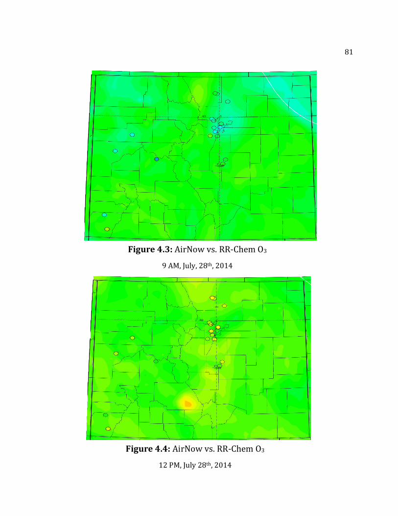
!
!
81!
Figure'4.3:'AirNow!vs.!RR6Chem!O3!9!AM,!July,!28th,!2014!
Figure'4.4:'AirNow!vs.!RR6Chem!O3!12!PM,!July!28th,!2014!

!
!
82!
Figure'4.5:'AirNow!vs.!RR6Chem!O3!3!PM,!July!28th,!2014!
Figure'4.6:'AirNow!vs.!RR6Chem!O3!6!PM,!July!28th,!2014!

!
!
83!
Figure'4.7:'AirNow!vs.!RR6Chem!O3!9!PM,!July!28th,!2014!

!
!
84!
Figure'4.8:'P3B!flight!track!on!July!28th,!2014!Source:(NASA(&(Google(Earth(
Figure'4.9:'P3B!in!situ!vs.!RR6Chem!HCHO!(black,!red)!and!altitude!(blue)!!July!28th,!2014!
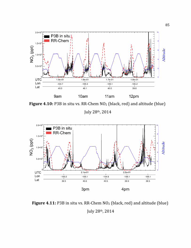
!
!
85!
Figure'4.10:'P3B!in!situ!vs.!RR6Chem!NO2!(black,!red)!and!altitude!(blue)!!July!28th,!2014!
Figure'4.11:'P3B!in!situ!vs.!RR6Chem!NO2!(black,!red)!and!altitude!(blue)!!July!28th,!2014!

!
!
86!
Figure'4.12:'P3B!in!situ!vs.!RR6Chem!O3!(black,!red)!and!altitude!(blue)!!July!28th,!2014!
Figure'4.13:'P3B!in!situ!vs.!RR6Chem!O3!(black,!red)!and!altitude!(blue)!!July!28th,!2014!

!
!
87!
Figure'4.14:'EPA!Ceilometer!vs.!RR6Chem!boundary!layer!height!at!BAO!Tower!

!
!
88!
Figure'4.15:'BAO!measurements!vs.!RR6Chem!O3!(dark!blue,!red)!and!RR6Chem!modeled!boundary!layer!height!(light!blue)!
Figure'4.16:'EPA!Ceilometer!measurements!at!vs.!RR6Chem!PBLH!(blue,!red)!at!BAO!Tower!

!
!
89!Chapter 4 References
Anderson, D. C., Loughner, C. P., Diskin, G., Weinheimer, A., Canty, T. P., Salawitch, R. J., … Dickerson, R. R. (2014). Measured and modeled CO and NOy in DISCOVER-AQ: An evaluation of emissions and chemistry over the eastern US. Atmospheric Environment, 96, 78–87. doi:10.1016/j.atmosenv.2014.07.004
Barth, M. C., Wong, J., Bela, M. M., Pickering, K. E., Li, Y., & Cummings, K. (2014). Simulations of L ightning - Generated NOx for Parameterized C onvection in the WRF - Chem model, 4(2), 15–20.
Charles, L. A., Chaw, S., Vladutescu, V., Wu, Y., Moshary, F., Gross, B., … Ahmed, S. (1970). Application Of CCNY Lidar And Ceilometers To The Study Of Aerosol Transport And PM2.5.
Czader, B. H., Li, X., & Rappenglueck, B. (2013). CMAQ modeling and analysis of radicals, radical precursors, and chemical transformations. Journal of Geophysical Research: Atmospheres, 118(19), 11376–11387. doi:10.1002/jgrd.50807
EPA, (2013). 2011 National Emissions Inventory, Version 1 Technical Support Document, (November).
Ghude, S. D., Pfister, G. G., Jena, C., Van Der A, R. J., Emmons, L. K., & Kumar, R. (2013). Satellite constraints of nitrogen oxide (NOx) emissions from India based on OMI observations and WRF-Chem simulations. Geophysical Research Letters, 40(2), 423–428. doi:10.1029/2012GL053926
Gross, B. M., Gan, C., Wu, Y., Moshary, F., & Ahmed, S. (n.d.). Remote sensing to improve air quality forecasts, 2–4.
Valin, L. C., Russell, a. R., Hudman, R. C., & Cohen, R. C. (2011). Effects of model resolution on the interpretation of satellite NO2 observations. Atmospheric Chemistry and Physics, 11(22), 11647–11655. doi:10.5194/acp-11-11647-2011
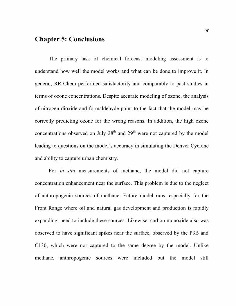
!
!
90!Chapter 5: Conclusions
The primary task of chemical forecast modeling assessment is to
understand how well the model works and what can be done to improve it. In
general, RR-Chem performed satisfactorily and comparably to past studies in
terms of ozone concentrations. Despite accurate modeling of ozone, the analysis
of nitrogen dioxide and formaldehyde point to the fact that the model may be
correctly predicting ozone for the wrong reasons. In addition, the high ozone
concentrations observed on July 28th and 29th were not captured by the model
leading to questions on the model’s accuracy in simulating the Denver Cyclone
and ability to capture urban chemistry.
For in situ measurements of methane, the model did not capture
concentration enhancement near the surface. This problem is due to the neglect
of anthropogenic sources of methane. Future model runs, especially for the
Front Range where oil and natural gas development and production is rapidly
expanding, need to include these sources. Likewise, carbon monoxide also was
observed to have significant spikes near the surface, observed by the P3B and
C130, which were not captured to the same degree by the model. Unlike
methane, anthropogenic sources were included but the model still

!
!
91!underestimated observed concentrations most likely due to the coarse horizontal
resolution.
Modeled formaldehyde saw a contrasting bias than that observed of
methane and carbon dioxide. Formaldehyde was modeled with greater
enhancement near the surface than what was observed in situ measurements.
This was apparent not only in the general aircraft statistics but also in the case
study. One limitation of this study was the comprehensiveness of volatile
organic compound analysis. Formaldehyde was the only representative for
VOC performance so future studies should seek to include a wider variety of
volatile organic compounds. The complex nature of VOC emissions in the
Front Range, particularly from the developing oil and natural gas industry,
warrants further investigation and model analysis.
Nitrogen dioxide performance in RR-Chem had the highest bias of any of
the variables analyzed. The model overpredicted by nearly three times the
observed concentrations on average. Past studies have attributed the bias to the
National Emissions Inventory’s handling of mobile emissions in urban
environments (Anderson et al., 2014; Chen et al., 2013). Despite this, the bias
we found was significantly higher than previous studies, many that used the
NEI 2005 and 2008 databases, leading to further questions of whether this is
due to the NEI 2011 database bias or a model bias (EPA, 2013). Indeed
!
!
92!Anderson (2014) hypothesized the CO to NOx ratios in the 2011 NEI database
would contribute to a greater bias than their findings using the NEI 2008
database. Our analysis of OMI tropospheric NO2 column throughout the United
States substantiate those previous works with very high model bias in urban
environments and slight underprediction in the more rural areas. Nitrogen
dioxides ability to decrease ozone concentrations, at relatively high amounts
compared to local VOC concentrations, point to the model generally correctly
predicting ozone for the wrong reasons. This in addition to other model physics,
may have contributed to the lower than observed ozone concentrations during
the case study.
The case study highlighted deficiencies in the model predictions during
high ozone events coupled with the manifestation of unique dynamic features in
the Front Range of Colorado. Modeled ozone was significantly underpredicted
during the two-day ozone event that was analyzed, an atypical bias considering
the generally good AirNow and RR-Chem comparison. This bias was
hypothesized to be due to the model’s inability to correctly model pollution
concentrations within the Denver Cyclone in addition to other dynamics that
acted on spatial scales smaller than the model’s horizontal resolution. The
boundary layer was investigated both generally and more intensely during the
case study time period. The model’s parameterized boundary layer was found to
!
!
93!capture the observed diurnal variations with little bias and temporal lag. The
slight temporal lag of the boundary may have contributed to incorrect
atmospheric pollutant concentrations in the late morning and early afternoon
during the case study. That being said, the boundary layer was both over and
underpredicted by the model during the case studying ruling it out as the source
of the errors in modeled concentrations of ozone during this time period.
The rapid population growth of the Front Range coupled with unique
dynamic flows and emissions merit further investigation and study of the area.
Despite the several deficiencies of the model, more accurate emission
inventories and a higher resolution model grid should greatly improve model
accuracy. The critical focus of model improvement should be working with the
National Emissions Inventory to conduct further assessment in improving
nitrogen oxide emissions that contribute to not only NO2 concentration
inaccuracies but also ozone concentration inaccuracies. The importance of field
missions like FRAPPE and DISCOVER-AQ has been highlighted, as they are
crucial in chemical forecast model assessment. One possible solution in
monitoring atmospheric pollutant concentrations on a more regular basis could
be to deploy drones that would not only save money but also generate more
continuous vertical measurements for model comparison (Basly et al., 2010).

!
!
94!Chapter 5 References
Anderson, D. C., Loughner, C. P., Diskin, G., Weinheimer, A., Canty, T. P., Salawitch, R. J., … Dickerson, R. R. (2014). Measured and modeled CO and NOy in DISCOVER-AQ: An evaluation of emissions and chemistry over the eastern US. Atmospheric Environment, 96, 78–87. doi:10.1016/j.atmosenv.2014.07.004
Basly, L., Wald, L., Basly, L., Wald, L., Laurini, R., Second, T., … Antipolis, S. (2010). Remote sensing and air quality in urban areas To cite this version#: Remote Sensing and Air Quality in Urban Areas, (May 2000).
Chen, D., Li, Q., Stutz, J., Mao, Y., Zhang, L., Pikelnaya, O., … Pollack, I. B. (2013). WRF-Chem simulation of NOx and O3 in the L.A. basin during CalNex-2010. Atmospheric Environment, 81(x), 421–432. doi:10.1016/j.atmosenv.2013.08.064
EPA. (2013). 2011 National Emissions Inventory, Version 1 Technical Support Document, (November).
Related Documents