Evaluating Statistical Models - Carnegie Mellon …cshalizi/402/lectures/03-evaluation/lecture-03.pdfEvaluating Statistical Models 36-402, Data Analysis 18 January 2011 Optional Readings:

Evaluating Statistical Models

36-402, Data Analysis

18 January 2011

Optional Readings: Berk, chapter 2.

Contents

1 What Are Statistical Models For? Summaries, Forecasts, Sim-ulators 1

2 Errors, In and Out of Sample 3

3 Over-Fitting and Model Selection 5

4 Cross-Validation 114.1 Data-set Splitting . . . . . . . . . . . . . . . . . . . . . . . . . . . 114.2 Cross-Validation (CV) . . . . . . . . . . . . . . . . . . . . . . . . 124.3 Leave-one-out Cross-Validation . . . . . . . . . . . . . . . . . . . 12

5 Warnings 13

6 Exercises 13

1 What Are Statistical Models For? Summaries,Forecasts, Simulators

There are (at least) three levels at which we can use statistical models in dataanalysis: as summaries of the data, as predictors, and as simulators.

The lowest and least demanding level is just to use the model as a summaryof the data — to use it for data reduction, or compression. Just as onecan use the sample mean or sample quantiles as descriptive statistics, recordingsome features of the data and saying nothing about a population or a gener-ative process, we could use estimates of a model’s parameters as descriptivesummaries. Rather than remembering all the points on a scatter-plot, say, we’djust remember what the OLS regression surface was.

It’s hard to be wrong about a summary, unless we just make a mistake. (Itmay or may not be helpful for us later, but that’s different.) When we say “the

1

slope which best fit the training data was b = 4.02”, we make no claims aboutanything but the training data. It relies on no assumptions, beyond our doingthe calculations right. But it also asserts nothing about the rest of the world.As soon as we try to connect our training data to the rest of the world, we startrelying on assumptions, and we run the risk of being wrong.

Probably the most common connection to want to make is to say what otherdata will look like — to make predictions. In a statistical model, with randomnoise terms, we do not anticipate that our predictions will ever be exactly right,but we also anticipate that our mistakes will show stable probabilistic patterns.We can evaluate predictions based on those patterns of error — how big is ourtypical mistake? are we biased in a particular direction? do we make a lot oflittle errors or a few huge ones?

Statistical inference about model parameters — estimation and hypothesistesting — can be seen as a kind of prediction, extrapolating from what we sawin a small piece of data to what we would see in the whole population, or wholeprocess. When we estimate the regression coefficient b = 4.02, that involvespredicting new values of the dependent variable, but also predicting that if werepeated the experiment and re-estimated b, we’d get a value close to 4.02.

Using a model to summarize old data, or to predict new data, doesn’t commitus to assuming that the model describes the process which generates the data.But we often want to do that, because we want to interpret parts of the modelas aspects of the real world. We think that in neighborhoods where people havemore money, they spend more on houses — perhaps each extra $1000 in incometranslates into an extra $4020 in house prices. Used this way, statistical modelsbecome stories about how the data were generated. If they are accurate, weshould be able to use them to simulate that process, to step through it andproduce something that looks, probabilistically, just like the actual data. Thisis often what people have in mind when they talk about scientific models, ratherthan just statistical ones.

An example: if you want to predict where in the night sky the planets willbe, you can actually do very well with a model where the Earth is at the centerof the universe, and the Sun and everything else revolve around it. You caneven estimate, from data, how fast Mars (for example) goes around the Earth,or where, in this model, it should be tonight. But, since the Earth is not at thecenter of the solar system, those parameters don’t actually refer to anything inreality. They are just mathematical fictions. On the other hand, we can alsopredict where the planets will appear in the sky using models where all theplanets orbit the Sun, and the parameters of the orbit of Mars in that model dorefer to reality.1

We are going to focus today on evaluating predictions, for three reasons.First, often we just want prediction. Second, if a model can’t even predict well,it’s hard to see how it could be right scientifically. Third, often the best wayof checking a scientific model is to turn some of its implications into statistical

1We can be pretty confident of this, because we use our parameter estimates to send ourrobots to Mars, and they get there.

2

predictions.

2 Errors, In and Out of Sample

With any predictive model, we can gauge how well it works by looking at itserrors. We want these to be small; if they can’t be small all the time we’dlike them to be small on average. We may also want them to be patternlessor unsystematic (because if there was a pattern to them, why not adjust forthat, and make smaller mistakes). We’ll come back to patterns in errors later,when we look at specification testing. For now, we’ll concentrate on how bigthe errors are.

To be a little more mathematical, we have a data set with points zn =z1, z2, . . . zn. (For regression problems, think of each data point as the pair ofinput and output values, so zi = (xi, yi), with xi possibly a vector.) We also havevarious possible models, each with different parameter settings, conventionallywritten θ. For regression, θ tells us which regression function to use, so mθ(x) orm(x; θ) is the prediction we make at point x with parameters set to θ. Finally,we have a loss function L which tells us how big the error is when we use acertain θ on a certain data point, L(z, θ). For mean-squared error, this wouldjust be

L(z, θ) = (y −mθ(x))2

But we could also use the mean absolute error

L(z, θ) = |y −mθ(x)|

or many other loss functions. Sometimes we will actually be able to measure howcostly our mistakes are, in dollars or harm to patients. If we had a model whichgave us a distribution for the data, then pθ(z) would a probability density atz, and a typical loss function would be the negative log-likelihood, − logmθ(z).No matter what the loss function is, I’ll abbreviate the sample average of theloss over the whole data set by L(zn, θ).

What we would like, ideally, is a predictive model which has zero error onfuture data. We basically never achieve this:

• The world just really is a noisy and stochastic place, and this means eventhe true, ideal model has non-zero error.2 If, in the usual linear regressionassumptions, Y = βX + ε, ε ∼ N (0, σ2), then σ2 sets a limit on how wellY can be predicted, and nothing will truly get the mean-squared errorbelow that limit.

• Our models are never perfectly estimated. Even if our data come from aperfect IID source, we only ever have a finite sample, and so our parameterestimates are (almost) never quite the true, infinite-limit values. This is

2This is so even if you believe in some kind of ultimate determinism, because the variableswe plug in to our predictive models are not complete descriptions of the physical state of theuniverse, but rather immensely coarser, and this coarseness shows up as randomness.

3

the origin of the variance term in the bias-variance decomposition. Butas we get more and more data, the sample should become more and morerepresentative of the whole process, and estimates should converge too.

• Our models are usually more or less mis-specified, or, in plain words,wrong. We hardly ever get the functional form of the regression, thedistribution of the exogenous noise, the form of the causal dependencebetween two factors, etc., exactly right.3 This is the origin of the biasterm in the bias-variance decomposition. Of course we can get any of thedetails in the model specification more or less wrong, and we’d prefer tobe less wrong.

So, because our models are flawed, we have limited data and the world is stochas-tic, we cannot expect even the best model to have zero error. Instead, we wouldlike to minimize the expected error, or risk, or generalization error, onnew data.

What we would like to do is to minimize the risk or expected loss

E [L(Z, θ)] =∫dzp(z)L(z, θ)

To do this, however, we’d have to be able to calculate that expectation. Doingthat would mean knowing the distribution of Z — the joint distribution ofX andY , for the regression problem. Since we don’t know the true joint distribution,we need to approximate it somehow.

A natural approximation is to use our training data zn. For each possiblemodel θ, we can could calculate the error on the data, L(zn, θ), called the in-sample loss or the empirical risk. The simplest strategy for estimation isthen to pick the model, the value of θ, which minimizes the in-sample loss. Thisstrategy is imaginatively called empirical risk minimization. Formally,

θn ≡ argminθ∈Θ

L(zn, θ)

This means picking the regression which minimizes the sum of squared errors,or the density with the highest likelihood4. This what you’ve usually done instatistics courses so far, and it’s very natural, but it does have some issues,notably optimism and over-fitting.

The problem of optimism comes from the fact that our training data isn’tperfectly representative. The in-sample loss is a sample average. By the law oflarge numbers, then, we anticipate that, for each θ,

L(zn, θ)→ E [L(Z, θ)]3Except maybe in fundamental physics, and even there our predictions are about our

fundamental theories in the context of experimental set-ups, which we never model in completedetail.

4Remember, maximizing the likelihood is the same as maximizing the log-likelihood, be-cause log is an increasing function. Therefore maximizing the likelihood is the same as mini-mizing the negative log-likelihood.

4

as n → ∞. This means that, with enough data, the in-sample error is a goodapproximation to the generalization error of any given model θ. (Big samplesare representative of the underlying population or process.) But this does notmean that the in-sample performance of θ tells us how well it will generalize,because we purposely picked it to match the training data zn. To see this, noticethat the in-sample loss equals the risk plus sampling noise:

L(zn, θ) = E [L(Z, θ)] + ηn(θ) (1)

Here η(θ) is a random term which has mean zero, and represents the effectsof having only a finite quantity of data, of size n, rather than the completeprobability distribution. (I write it ηn(θ) as a reminder that different modelsare going to be affected differently by the same sampling fluctuations.) Theproblem, then, is that the model which minimizes the in-sample loss could beone with good generalization performance (E [L(Z, θ)] is small), or it could beone which got very lucky (ηn(θ) was large and negative):

θn = argminθ∈Θ

(E [L(Z, θ)] + ηn(θ)) (2)

We only want to minimize E [L(Z, θ)], but we can’t separate it from ηn(θ), sowe’re almost surely going to end up picking a θn which was more or less lucky(ηn < 0) as well as good (E [L(Z, θ)] small). This is the reason why picking themodel which best fits the data tends to exaggerate how well it will do in thefuture.

Again, by the law of large numbers ηn(θ) → 0 for each θ, but now we needto worry about how fast it’s going to zero, and whether that rate depends onθ. Suppose we knew that minθ ηn(θ) → 0, or maxθ |ηn(θ)| → 0. Then it wouldfollow that ηn(θn) → 0, and the over-optimism in using the in-sample error toapproximate the generalization error would at least be shrinking. If we knewhow fast maxθ |ηn(θ)| was going to zero, we could even say something about howmuch bigger the true risk was likely to be. A lot of more advanced statistics andmachine learning theory is thus about uniform laws of large numbers (showingmaxθ |ηn(θ)| → 0) and rates of convergence.

Learning theory is a beautiful, deep, and practically important subject, butalso subtle and involved one.5 To stick closer to analyzing real data, and tonot turn this into an advanced probability class, I will only talk about somemore-or-less heuristic methods, which are good enough for many purposes.

3 Over-Fitting and Model Selection

The big problem with using the in-sample error is related to over-optimism, butat once trickier to grasp and more important. This is the problem of over-fitting. To illustrate it, let’s start with Figure 1. This has the twenty X values

5Some comparatively easy starting points are Kearns and Vazirani (1994) or Cristianiniand Shawe-Taylor (2000). At a more advanced level, look at the tutorial papers by Bousquetet al. (2004); von Luxburg and Scholkopf (2008), or the textbook by Vidyasagar (2003), orread the book by Vapnik (2000) (one of the founders), or take the class 10-702.

5

from a Gaussian distribution, and Y = 7X2 − 0.5X + ε, ε ∼ N (0, 1). That is,the true regression curve is a parabola, with additive and independent Gaussiannoise. Let’s try fitting this — but pretend that we didn’t know that the curvewas a parabola. We’ll try fitting polynomials of different orders in x — order0 (a flat line), order 1 (a linear regression), order 2 (quadratic regression), upthrough order 9. Figure 3 shows the data with the polynomial curves, andFigure 3 shows the in-sample mean squared error as a function of the order ofthe polynomial.

Notice that the in-sample error goes down as the order of the polynomialincreases; it has to. Every polynomial of order p is also a polynomial of orderp+1, so going to a higher-order model can only reduce the in-sample error. Quitegenerally, in fact, as one uses more and more complex and flexible models, thein-sample error will get smaller and smaller.6

Things are quite different if we turn to the generalization error. In principle,I could calculate that for any of the models, since I know the true distribution,but it would involve calculating things like E

[X18

], which won’t be very illumi-

nating. Instead, I will just draw a lot more data from the same source, twentythousand data points in fact, and use the error of the old models on the newdata as their generalization error. The results are in Figure 4.

What is happening here is that the higher-order polynomials — beyond order2 — are not just a bit optimistic about how well they fit, they are wildly over-optimistic. The models which seemed to do notably better than a quadraticactually do much, much worse. If we picked a polynomial regression modelbased on in-sample fit, we’d chose the highest-order polynomial available, andsuffer for it.

What’s going on here is that the more complicated models — the higher-order polynomials, with more terms and parameters — were not actually fittingthe generalizable features of the data. Instead, they were fitting the samplingnoise, the accidents which don’t repeat. That is, the more complicated modelsover-fit the data. In terms of our earlier notation, η is bigger for the moreflexible models. The model which does best here is the quadratic, becausethe true regression function happens to be of that form. The more powerful,more flexible, higher-order polynomials were able to get closer to the trainingdata, but that just meant matching the noise better. In terms of the bias-variance decomposition, the bias shrinks with the model order, but the varianceof estimation grows.

Notice that the models of order 0 and order 1 also do worse than thequadratic model — their problem is not over-fitting but under-fitting; theywould do better if they were more flexible. Plots of generalization error likethis usually have a minimum. If we have a choice of models — if we need todo model selection — we would like to find the minimum. Even if we do nothave a choice of models, we might like to know how big the gap between ourin-sample error and our generalization error is likely to be.

6In fact, since there are only 20 data points, they could all be fit exactly if the order of thepolynomials went up to 19. (Remember that any two points define a line, any three points aparabola, etc. — p + 1 points define a polynomial of order p which passes through them.)

6

-2 -1 0 1 2

010

2030

4050

x

y

plot(x,y2)curve(7*x^2-0.5*x,add=TRUE,col="grey")

Figure 1: Scatter-plot showing sample data and the true, quadratic regressioncurve (grey parabola).

7

-2 -1 0 1 2

010

2030

4050

x

y

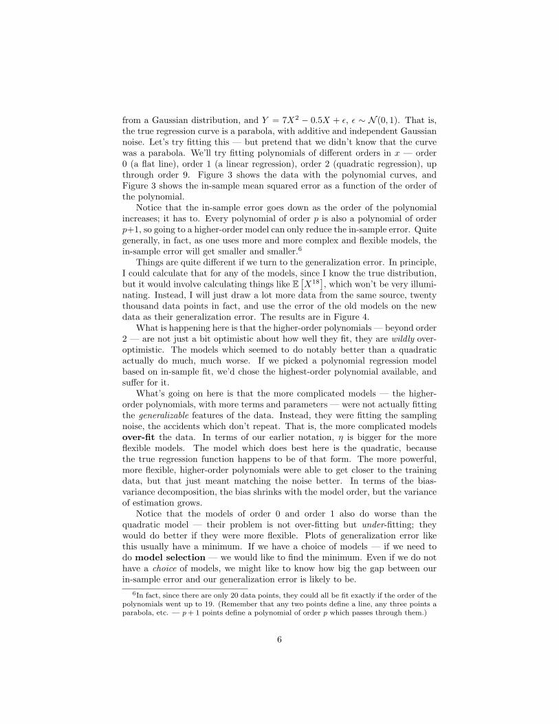
y2.0 = lm(y2 ~ 1)abline(h=y2.0$coefficients[1])d = seq(-2,2,length.out=200)for (degree in 1:9) {fm = lm(y2 ~ poly(x,degree))assign(paste("y2",degree,sep="."), fm)lines(d, predict(fm,data.frame(x=d)),lty=(degree+1))

}

Figure 2: Twenty training data points (dots), and ten different fitted regressionlines (polynomials of order 0 to 9, indicated by different line types). R notes:The poly command constructs orthogonal (uncorrelated) polynomials of the specifieddegree from its first argument; regressing on them is conceptually equivalent to re-gressing on 1, x, x2, . . . xdegree, but more numerically stable. (See help(poly).) Thisuse of the assign and paste functions together is helpful for storing results whichdon’t fit well into arrays.

8

0 2 4 6 8

0.5

1.0

2.0

5.0

10.0

20.0

50.0

100.0

polynomial degree

mea

n sq

uare

d er

ror

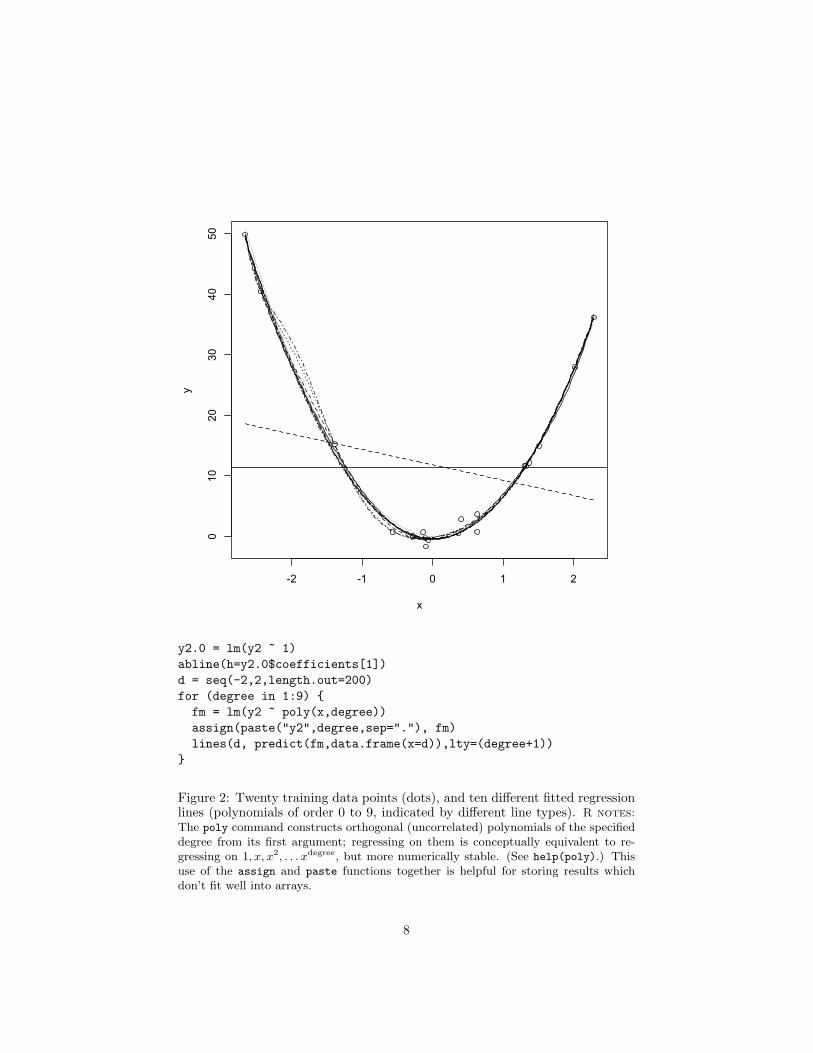
mse.q = vector(length=10)for (degree in 0:9) {# The get() function is the inverse to assign()fm = get(paste("y",degree,sep="."))mse.q[degree+1] = mean(residuals(fm)^2)

}plot(0:9,mse.q,type="b",xlab="polynomial degree",ylab="mean squared error",

log="y")

Figure 3: Degree of polynomial vs. its in-sample mean-squared error on thedata from the previous figure. Note the logarithmic scale for the vertical axis.

9

0 2 4 6 8

0.5

1.0

2.0

5.0

10.0

20.0

50.0

100.0

polynomial degree

mea

n sq

uare

d er

ror

gmse.q = vector(length=10)for (degree in 0:9) {fm = get(paste("y",degree,sep="."))predictions = predict(fm,data.frame(x=x.new))resids = y.new - predictionsgmse.q[degree+1] = mean(resids^2)

}plot(0:9,mse.q,type="b",xlab="polynomial degree",

ylab="mean squared error",log="y",ylim=c(min(mse.q),max(gmse.q)))lines(0:9,gmse.q,lty=2,col="blue")points(0:9,gmse.q,pch=24,col="blue")

Figure 4: In-sample error (black dots) compared to generalization error (bluetriangles). Note the logarithmic scale for the vertical axis.

10

There is nothing special about polynomials here. All of the same lessonsapply to variable selection in linear regression, to k-nearest neighbors (where weneed to choose k), to kernel regression (where we need to choose the bandwidth),and to other methods we’ll see later. In every case, there is going to be aminimum for the generalization error curve, which we’d like to find.

(A minimum with respect to what, though? In Figure 4, the horizontal axisis the model order, which here is the number of parameters (minus one). Moregenerally, however, what we care about is some measure of how complex themodel space is, which is not necessarily the same thing as the number of pa-rameters. What’s more relevant is how flexible the class of models is, how manydifferent functions it can approximate. Linear polynomials can approximate asmaller set of functions than quadratics can, so the latter are more complex, orhave higher capacity. More advanced learning theory has a number of waysof quantifying this, but the details are pretty arcane, so we will just use theconcept of complexity or capacity informally.)

4 Cross-Validation

The most straightforward way to find the generalization error would be to dowhat I did above, and to use fresh, independent data from the same source — atesting or validation data-set. Call this z′m, as opposed to our training datazn. We fit our model to zn, and get θn. The loss of this on the validation datais

E[L(Z, θn)

]+ η′m(θn)

where now the sampling noise on the validation set, η′m, is independent of θm.So this gives us an unbiased estimate of the generalization error, and, if m islarge, a precise one. If we need to select one model from among many, we canpick the one which does best on the validation data, with confidence that weare not just over-fitting.

The problem with this approach is that we absolutely, positively, cannotuse any of the validation data in estimating the model. Since collecting data isexpensive — it takes time, effort, and usually money, organization and skill —this means getting a validation data set is expensive, and we often won’t havethat luxury.

4.1 Data-set Splitting

The next logical step, however, is to realize that we don’t strictly need a separatevalidation set. We can just take our data and split it ourselves into trainingand testing sets. If we divide the data into two parts at random, we ensurethat they have (as much as possible) the same distribution, and that they areindependent of each other. Then we can act just as though we had a realvalidation set. Fitting to one part of the data, and evaluating on the other,gives us an unbiased estimate of generalization error.

11

4.2 Cross-Validation (CV)

The problem with data-set splitting is that, while it’s an unbiased estimate ofthe risk, it is often a very noisy one. If we split the data evenly, then thetest set has n/2 data points — we’ve cut in half the number of sample pointswe’re averaging over. It would be nice if we could reduce that noise somewhat,especially if we are going to use this for model selection.

One solution to this, which is pretty much the industry standard, is what’scalled k-fold cross-validation. Pick a small integer k, usually 5 or 10, anddivide the data at random into k equally-sized subsets. (The subsets are some-times called “folds”.) Take the first subset and make it the test set; fit themodels to the rest of the data, and evaluate their predictions on the test set.Now make the second subset the test set and the rest of the training sets. Repeatuntil each subset has been the test set. At the end, average the performanceacross test sets. This is the cross-validated estimate of generalization error foreach model. Model selection then picks the model with the smallest estimatedrisk.7

The reason cross-validation works is that it uses the existing data to simulatethe process of generalizing to new data. If the full sample is large, then eventhe smaller portion of it in the training data is, with high probability, fairlyrepresentative of the data-generating process. Randomly dividing the data intotraining and test sets makes it very unlikely that the division is rigged to favorany one model class, over and above what it would do on real new data. Ofcourse the original data set is never perfectly representative of the full data,and a smaller testing set is even less representative, so this isn’t ideal, but theapproximation is often quite good.

Cross-validation is probably the most widely-used method for model selec-tion, and for picking control settings, in modern statistics. There are circum-stances where it can fail — especially if you give it too many models to pickamong — but it’s the first thought of seasoned practitioners, and it should beyour first thought, too. The homework to come will make you very familiar withit.

4.3 Leave-one-out Cross-Validation

Suppose we did k-fold cross-validation, but with k = n. Our testing sets wouldthen consist of single points, and each point would be used in testing once.This is called leave-one-out cross-validation. It actually came before k-foldcross-validation, and has two advantages. First, it doesn’t require any randomnumber generation, or keeping track of which data point is in which subset.Second, and more importantly, because we are only testing on one data point,it’s often possible to find what the prediction on the left-out point would be by

7A closely related procedure, sometimes also called “k-fold CV”, is to pick 1/k of thedata points at random to be the test set (using the rest as a training set), and then pick anindependent 1/k of the data points as the test set, etc., repeating k times and averaging. Thedifferences are subtle, but what’s described in the main text makes sure that each point isused in the test set just once.

12

doing calculations on a model fit to the whole data. This means that we onlyhave to fit each model once, rather than k times, which can be a big savings ofcomputing time.

The drawback to leave-one-out CV is subtle but often decisive. Since eachtraining set has n−1 points, any two training sets must share n−2 points. Themodels fit to those training sets tend to be strongly correlated with each other.Even though we are averaging n out-of-sample forecasts, those are correlatedforecasts, so we are not really averaging away all that much noise. With k-foldCV, on the other hand, the fraction of data shared between any two trainingsets is just k−2

k−1 , not n−2n−1 , so even though the number of terms being averaged

is smaller, they are less correlated.There are situations where this issue doesn’t really matter, or where it’s

overwhelmed by leave-one-out’s advantages in speed and simplicity, so there iscertainly still a place for it, but one subordinate to k-fold CV.

5 Warnings

Some caveats are in order.

1. All the model selection methods we have discussed aim at getting modelswhich predict well. This is not necessarily the same as getting the truetheory of the world. Presumably the true theory will also predict well,but the converse does not necessarily follow. We will see examples laterwhere false but low-capacity models, because they have such low varianceof estimation, actually out-predict correctly specified models.

2. All of these model selection methods aim at getting models which willgeneralize well to new data, if it follows the same distribution as old data.Generalizing well even when distributions change is a much harder andmuch less well-understood problem (Quinonero-Candela et al., 2009). Itis particularly troublesome for a lot of applications involving large num-bers of human beings, because society keeps changing all the time — it’snatural for the variables to vary, but the relationships between variablesalso changes. (That’s history.)

6 Exercises

To think through, not to hand in.

1. Suppose that one of our model classes contains the true and correct model,but we also consider more complicated and flexible model classes. Doesthe bias-variance trade-off mean that we will over-shoot the true model,and always go for something more flexible, when we have enough data?(This would mean there was such a thing as too much data to be reliable.)

13

References

Bousquet, Olivier, Stephane Boucheron and Gabor Lugosi (2004). “Introductionto Statistical Learning Theory.” In Advanced Lectures in Machine Learning(Olivier Bousquet and Ulrike von Luxburg and Gunnar Ratsch, eds.), pp. 169–207. Berlin: Springer-Verlag. URL http://www.econ.upf.edu/~lugosi/mlss_slt.pdf.

Cristianini, Nello and John Shawe-Taylor (2000). An Introduction to SupportVector Machines: And Other Kernel-Based Learning Methods. Cambridge,England: Cambridge University Press.

Kearns, Michael J. and Umesh V. Vazirani (1994). An Introduction to Compu-tational Learning Theory . Cambridge, Massachusetts: MIT Press.

Quinonero-Candela, Joaquin, Masashi Sugiyama, Anton Schwaighofer andNeil D. Lawrence (eds.) (2009). Dataset Shift in Machine Learning . Cam-bridge, Massachusetts: MIT Press.

Vapnik, Vladimir N. (2000). The Nature of Statistical Learning Theory . Berlin:Springer-Verlag, 2nd edn.

Vidyasagar, M. (2003). Learning and Generalization: With Applications toNeural Networks. Berlin: Springer-Verlag, 2nd edn.

von Luxburg, Ulrike and Bernhard Scholkopf (2008). “Statistical LearningTheory: Models, Concepts, and Results.” E-print, arxiv.org. URL http://arxiv.org/abs/0810.4752.

14