Evaluating short-term morphological changes in a gravel-bed braided river using terrestrial laser scanner

Geomorphology 201 (2013) 323–334

Contents lists available at ScienceDirect

Geomorphology

j ourna l homepage: www.e lsev ie r .com/ locate /geomorph

Evaluating short-term morphological changes in a gravel-bed braidedriver using terrestrial laser scanner

L. Picco a,⁎, L. Mao b, M. Cavalli c, E. Buzzi a, R. Rainato a, M.A. Lenzi a

a Department of Land, Environment, Agriculture and Forestry, University of Padova, Padova, Italyb Department of Ecosystems and Environment, Pontificia Universidad Catolica de Chile, Santiago, Chilec CNR-IRPI, Corso Stati Uniti 4, 35127 Padova, Italy

⁎ Corresponding author. Tel.: +39 0498272695; fax:E-mail address: [email protected] (L. Picco).

0169-555X/$ – see front matter © 2013 Elsevier B.V. Alhttp://dx.doi.org/10.1016/j.geomorph.2013.07.007

a b s t r a c t

Article history:Received 21 April 2012Received in revised form 4 July 2013Accepted 6 July 2013Available online 16 July 2013

Keywords:Gravel-bed braided riverTagliamento RiverTerrestrial laser scannerMorphological changesGeomorphic change detectionRoughness

Braided rivers are dynamic and complex environments shaped by the balance of the flow and sedimentregimes and by the influence of the riparian vegetation and disturbances such as floods. In particular, the bal-ance between sediment supply and transport capacity can determine the morphological evolution of a river.For instance, aggrading and widening trends are distinctive of reaches where sediment supply is higher thantransport capacity. In contrast, incising and narrowing tendencies are dominant. The aim of the present studyis to analyze the short-term morphological dynamics and the processes of erosion and sediment depositionalong a small reach of a relatively unimpacted gravel-bed braided river (Tagliamento River, northeast Italy)using a terrestrial laser scanner (TLS). The study area is around 23 ha and has been surveyed before aftertwo periods with relevant flood events, two of which were higher than the bankfull level and occurred be-tween September 2010 and September 2011. The very high point clouds density allowed us to derive threehigh resolution digital elevation models (DEMs) with 0.125 × 0.125 m pixel size. Scan data cloud mergingwas achieved with an overall high degree of accuracy and resolution (subcentimeter). Topographic datawere more accurate for exposed surfaces than those collected in wet areas. A detailed net of dGPS controlpoints allowed us to verify the high quality of the DEMs derived from the surveys (RMSE of about 5 cm).Two DEMs of difference (DoD) were computed, revealing different and consistent episodes of erosion and de-position within the analyzed area, and changes in morphology of channel and bars could also be detected,such as bar edge accretion and bank erosion demonstrating a strong dynamicity of the Tagliamento River.Moreover, a very detailed estimation of the surface roughness in the study area has been carried out, permit-ting a large-scale analysis of the roughness values distribution. The results of the analysis on the TLS collecteddata show that along a river with a high natural character (i.e., Tagliamento River), the dynamic processes arealso common during low magnitude events.

© 2013 Elsevier B.V. All rights reserved.

1. Introduction

Braided rivers are characterized by flowing in at least two alluvialchannels, separated by bars and islands as to produce a multithreadedplatform (Leopold and Wolman, 1957). These fluvial systems are themost dynamic among alluvial rivers (Brierley and Fryirs, 2005). Braid-ing, from a hypothetical straight channel, occurs by four different pro-cesses: deposition and accumulation of a central bar, chute cutoff ofpoint bars, conversion of single transverse unit bars to mid-channelbraid bars, and dissection of multiple bars (Ashmore, 1991). A highmorphological complexity arises from the coexistence of several spatialstructures, controlled by different spatiotemporal scales interacting inthe development of the braided pattern, giving rise to strong fluctua-tions both in time and in space (Bertoldi et al., 2009). Gravel-bed braid-ed rivers are very dynamic systems and in this context even ordinary

+39 0498272686.

l rights reserved.

flood events can triggermorphologically active processes. Channel evo-lution is a response to fluctuations and changes of runoff and sedimentsupply involvingmutual interactions among channel form, bedmaterialsize, hydraulic forces (Lisle et al., 2000), riparian vegetation (Picco et al.,2012b), and islands (Picco et al., 2012a).

Field studies provided an important insight into braided rivermechanics (Ashworth and Ferguson, 1986; Ashworth et al., 1992;Ferguson et al., 1992), but these investigations have suffered frompoor spatial and temporal sampling resolution of hydraulic, morpho-logic, sediment transport, and bed grain size variables (Ferguson,1993). During the early 1990s, several studies based on field investi-gations were focused on processes occurring at the chute-bar, orconfluence scale (Ashworth et al., 1992; Ferguson et al., 1992; Laneand Richards, 1998). Recent advances in survey equipment and soft-ware allowed high resolution digital elevation models (DEMs) to beconstructed. This new generation of DEMs is able to represent accu-rately earth's surface (Tarolli et al., 2009) and offers an excellent op-portunity to measure and monitor morphological change across a

324 L. Picco et al. / Geomorphology 201 (2013) 323–334

variety of spatial scales (Brasington et al., 2000; Lane and Chandler,2003; Heritage and Hetherington, 2007; Hicks et al., 2007; Fulleret al., 2009). Coupled with this, the development of topographic sur-vey techniques, i.e., airborne and terrestrial LiDAR (light detectionand ranging), electronic distance measuring device (EDM) theodo-lites, global positioning system (GPS), photogrammetry, and spec-trally based bathymetry has led to an increase in the amount ofdata collected during fieldwork in a riverine environment, offeringnew insights into fluvial dynamics (Lane et al., 1994; Milne andSear, 1997; Heritage et al., 1998; Brasington et al., 2000; Heritageand Hetherington, 2007; Marcus and Fonstad, 2008; Fuller et al.,2009). Developments in the methods used to obtain high resolutionmorphological data sets in river environments include synoptic remotesensing (Lane et al., 2003), CDW (close range digital workstation) pho-togrammetry at the bar scale (Heritage et al., 1998), photogrammetry influmes (Ashmore et al., 2000; Lindsay and Ashmore, 2002; Marcus andFonstad, 2008), total station survey (Fuller et al., 2003, 2009), surveysusing real time kinematic GPS (RTK-GPS) (Brasington et al., 2000,2003), airborne LiDAR (Thoma et al., 2005; Cavalli et al., 2008; Höfleet al., 2009; Cavalli and Tarolli, 2011;Moretto et al., 2012), and terrestri-al laser scanner (TLS) (Williams et al., 2011). Among the mentionedtechniques, airborne LiDAR (Charlton et al., 2003; French, 2003) offersthe possibility to carry out fast and accurate topographic surveysof large areas at a relatively affordable cost. Different authors haveshown that, thanks to the advances in the survey technologies, duringthe last years there was a remarkable increase in spatial extent and res-olution related to topographic data acquisition (Lane and Chandler,2003; Heritage and Hetherington, 2007; Milan et al., 2007; Marcusand Fonstad, 2008; Notebaert et al., 2009; Wheaton et al., 2010a).These advances make monitoring geomorphic changes and estimatingsediment budgets through repeat topographic surveys and the applica-tion of the morphological method (Church and Ashmore, 1998) a trac-table, affordable approach for monitoring applications in both researchand practice.

The calculation of difference between subsequent DEMs (differenceof DEMs, DoD) is a commonly applied method to analyze and quantifychannel change. It allows us to analyze, with a high level of resolution,topographic and volumetric changes during a certain time interval(Brasington et al., 2003; Rumsby et al., 2008) and to identify areas ofscour and fill (Lane et al., 2003). The DoDs also allow us to assesschanges in sediment storage, to improve sediment budget analysis atthe reach scale (e.g., Merz et al., 2006), and to study fluvial processes(Wheaton et al., 2010b). Most of the studies based on the DoD analysisare relative to temporal scales shorter than a decade because of the re-cent field survey made with improved remote sensing techniques(Heritage et al., 2009). Unfortunately, the computation of DoDs is usual-ly biased by different sources of uncertainty that strongly influencethe calculation of depositional and erosional volumes (Wheaton,

Fig. 1. The Tagliamento River basin (on the left), the study area localization (in the middle

2008). In fact, DEMs are affected by errors such as point quality, sam-pling strategy, surface composition, topographic complexity, and in-terpolation methods (Lane et al., 1994; Lane, 1998; Wise, 1998;Wechsler, 2003; Hancock, 2006; Wechsler and Kroll, 2006; Wise,2007). An approach to assessing spatially variable uncertainty inDoDs was presented by Wheaton et al. (2010a,b) and is based onthe creation of a fuzzy inference system (FIS) that permits us to com-bine individually errors of different sources. Heritage et al. (2009)and Milan et al. (2011) also developed a method to assess uncertaintybased on the surface roughness. Heritage et al. (2009) and Wheatonet al. (2010a, b) showed that the higher uncertainty values are obtainedin areaswith higher topographic variability and lower point density. Onthe other hand, flat areas with high point density featured the lowestuncertainty. The aims of the present research are (i) to recognize andassess the morphological changes occurred over two short periodscharacterized by ordinary flood events along a subreach of a low im-pacted gravel-bed braided river (Tagliamento River, Italy); (ii) to devel-op a novel approach with the fuzzy inference system to improve thechange detection analysis using TLS technology; and (iii) to derivesurface roughness maps along different geomorphic units from highlydetailed surveys.

2. Study area

The Tagliamento River is located in the southern Alps of northeastItaly. Its headwater originates at 1195 m above sea level (asl) andflows for 178 km to the northern Adriatic Sea, thus forming a linkingcorridor between Alpine and Mediterranean zones. Its drainage basincovers 2871 km2 (Fig. 1). The river has a straight course in the upperpart, while most of its course is braided shifting to meandering in thelower part where dykes have constrained the lower 30 km, so thatit is now little more than an artificial channel about 175 m wide.However, the upper reaches are mostly intact, so basic river processes(e.g., flooding or erosion and accumulation of sediment) take placeunder near natural conditions. A strong climate gradient exists alongthe length of the river that has great influence on precipitation, temper-ature, humidity, and consequently vegetation patterns. Because ofthe climate gradient, the floodplain of Tagliamento is an importantbiogeograpghical corridor with strong longitudinal, lateral and verticalconnectivity, and high habitat heterogeneity, a characteristic sequenceof geomorphic types and a very high biodiversity (Tockner et al., 2003).

The hydraulic regime, connected to the climatic and geologic con-ditions of the upper part, is characterized by flashy pluvio-nival flowconditions (Tockner et al., 2003). The Tagliamento River is consideredby different authors as the most intact and natural river in the Alps(Lippert et al., 1995; Müller, 1995; Ward et al., 1999), and it can beconsidered not only as ‘a reference ecosystem for the Alps but alsoas a model ecosystem for large temperate rivers' (Tockner et al.,

), and the entire study area analyzed (on the right). Flow direction is down the page.

Fig. 2. Flood events occurred during the study period along the Tagliamento River (on the left) and duration curves of the two periods considered in this study.

325L. Picco et al. / Geomorphology 201 (2013) 323–334

2003). The extensive vegetated islands and gravel bars are key indica-tors of its natural conditions, while engineering works for flood controlor navigation have lead to their disappearance in most comparableEuropean water courses. The Tagliamento River is clearly an ecosystemof European importance because it constitutes a unique resource as amodel reference catchment (Tockner et al., 2003).

The basins of the main tributaries of the upper catchments lie inone of the wettest region of Europe where annual precipitation canreach 3000 mm. The Tagliamento River is characterized by a bimodalflow regimewithmaximumdischarges in spring and autumndependingon snowmelt and intense rainfall in autumn, respectively. The catch-ment is mainly mountainous and the slopes are very steep, leading tohigh peak flows and sediment loads in the central and lower parts ofthe basin. The flood peak moves downstream very fast and can reachthe village of Latisana (on the regulated lower part) in just 12 h.Upstream, the height of the river rises by only 2 m, while nearthe Latisana village the river is compelled into a narrow channeland can rise to levels higher than 7 m.

Surveys have been made on about 23 ha located along a piedmontstretch of the Tagliamento River in a floodplain called Campo di Osoppo(Udine Province) (Fig. 1). This floodplain consists of a sedimentary layerwith a quite pronounced grain size variability (from fine sand to largepebbles). In this stretch the river has a braided channel configurationwith a significant presence of side bars, longitudinal bars, and islands.Islands have been colonized by stands of willow trees that have reachedthe maximum age of 5–7 years.

During the study period, different flood events were recordedalong the Tagliamento River. Between the first and second scan acqui-sition (see next section) there were three significant floods of around1 year recurrence interval, while between the second and the thirdscan acquisition there were five relevant flood events, two of whichwere higher than the bankfull level (Fig. 2).

3. Material and methods

3.1. TLS Topography acquisition and digital terrain model(DTM) derivation

Three surveys of the study area (T1, T2, and T3 in Table 1) werecarried out over 12 months using a Leica ScanStation2 TLS. The TLS

Table 1Main characteristics of data acquisitions.

Survey Period Duration Number of scans

T1 20–24 August 2010 5 days 21T2 18–22 October 2010 5 days 38T3 6–9 September 2011 4 days 27

used is a time-of-flight (first return) with high speed dual-axis com-pensator, characterized by precision of 6 mm on position and 4 mmon distance (for 100-m scan radius), range up to 150 m, scan speedup to 50,000 points per second, and maximum scan density b1 mm.To survey the entire study area, several scans were necessary (seeTable 1), depending on the complexity of the topographic surfaceand the presence of large wood (LW) jams or single logs. Therefore,a single survey required about 4–5 days of field work. We surveyedthe study area during periods with the same discharge level for T1and T2, whereas during T3 the channels in the study area were virtu-ally dry. Along the submerged areas, a differential global positioningsystem (dGPS) was used to collect ground data as the TLS data isnot accurate for the submerged areas (Milan et al., 2007). We mea-sured 241 and 2219 points for the T1 and T2 surveys, respectively.Nevertheless, the point density in wet areas was lower than that usu-ally achievable in dry areas using TLS.

Individual scans were registered, georeferenced, and filtered by re-moving LW to obtain only ground points. We carried out all these oper-ations using the Cyclone 7 software, developed by Cyra TechnologiesInc. The main characteristics of the three data acquisitions are listed inTable 1.

The study reach was virtually free of vegetation but featured threesingle logs along its downstream end. These logs were filtered manu-ally from the data set.

Filtered point clouds were imported into ArcGIS 10.1 (ESRI) as amultipoint shape file. Those data sets were merged with the pointscollected along the submerged areas using dGPS and with some air-borne LiDAR data in the right floodplain. LiDAR data were collectedin the same period of the TLS survey and georeferenced on thesame control network (stable points along the floodplain). Vectorialdata were interpolated using a natural neighbor algorithm with a res-olution of 0.125 m, which is comparable with the D84 of the area(Mao et al., in preparation).

Root mean square error (RMSE) analysis was conducted to definethe DTM vertical accuracy using a series of dGPS data (vertical qualitylower than 0.02 m) as control points. The errors were computed asthe difference between the control point elevation and the cell eleva-tion value in the DEM. The RMSE analysis resulted in the followingvalues: 0.052 on DTM T1 (August 2010), 0.053 on DTM T2 (October2010), and 0.048 on DTM T3 (September 2011), depicting the high

Point density (point/m2) Scan radius Surveyed area

74 Variable, from 70 to 120 m 23.3 ha122 Variable, from 70 to 120 m 23.3 ha221 150 m 23.3 ha

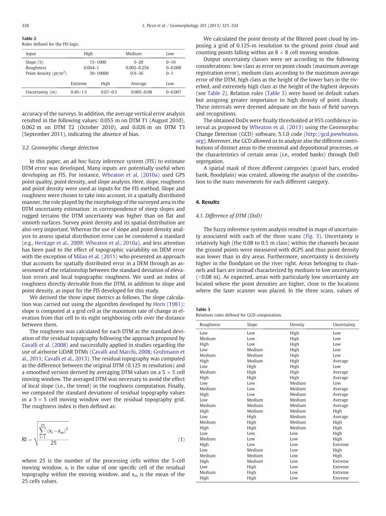
Table 2Rules defined for the FIS logic.

Input High Medium Low

Slope (%) 15–1000 5–20 0–10Roughness 0.064–1 0.002–0.256 0–0.008Point density (pt/m2) 30–10000 0.9–36 0–1

Extreme High Average Low

Uncertainty (m) 0.45–1.5 0.07–0.5 0.005–0.08 0–0.007

Table 3Relations rules defined for GCD computation.

Roughness Slope Density Uncertainty

Low Low High LowMedium Low High LowHigh Low High LowLow Medium High LowMedium Medium High LowHigh Medium High AverageLow High High LowMedium High High AverageHigh High High AverageLow Low Medium LowMedium Low Medium AverageHigh Low Medium AverageLow Medium Medium AverageMedium Medium Medium AverageHigh Medium Medium HighLow High Medium AverageMedium High Medium HighHigh High Medium HighLow Low Low HighMedium Low Low HighHigh Low Low ExtremeLow Medium Low HighMedium Medium Low HighHigh Medium Low ExtremeLow High Low ExtremeMedium High Low ExtremeHigh High Low Extreme

326 L. Picco et al. / Geomorphology 201 (2013) 323–334

accuracy of the surveys. In addition, the average vertical error analysisresulted in the following values: 0.055 m on DTM T1 (August 2010),0.062 m on DTM T2 (October 2010), and 0.026 m on DTM T3(September 2011), indicating the absence of bias.

3.2. Geomorphic change detection

In this paper, an ad hoc fuzzy inference system (FIS) to estimateDTM error was developed. Many inputs are potentially useful whendeveloping an FIS. For instance, Wheaton et al. (2010a) used GPSpoint quality, point density, and slope analysis. Here, slope, roughnessand point density were used as inputs for the FIS method. Slope androughness were chosen to take into account, in a spatially distributedmanner, the role played by themorphology of the surveyed area in theDTM uncertainty estimation: in correspondence of steep slopes andrugged terrains the DTM uncertainty was higher than on flat andsmooth surfaces. Survey point density and its spatial distribution arealso very important. Whereas the use of slope and point density anal-ysis to assess spatial distribution error can be considered a standard(e.g., Heritage et al., 2009; Wheaton et al., 2010a), and less attentionhas been paid to the effect of topographic variability on DEM errorwith the exception of Milan et al. (2011) who presented an approachthat accounts for spatially distributed error in a DEM through an as-sessment of the relationship between the standard deviation of eleva-tion errors and local topographic roughness. We used an index ofroughness directly derivable from the DTM, in addition to slope andpoint density, as input for the FIS developed for this study.

We derived the three input metrics as follows. The slope calcula-tion was carried out using the algorithm developed by Horn (1981):slope is computed at a grid cell as the maximum rate of change in el-evation from that cell to its eight neighboring cells over the distancebetween them.

The roughness was calculated for each DTM as the standard devi-ation of the residual topography following the approach proposed byCavalli et al. (2008) and successfully applied in studies regarding theuse of airborne LiDAR DTMs (Cavalli and Marchi, 2008; Grohmann etal., 2011; Cavalli et al., 2013). The residual topography was computedas the difference between the original DTM (0.125 m resolution) anda smoothed version derived by averaging DTM values on a 5 × 5 cellmoving window. The averaged DTMwas necessary to avoid the effectof local slope (i.e., the trend) in the roughness computation. Finally,we computed the standard deviations of residual topography valuesin a 5 × 5 cell moving window over the residual topography grid.The roughness index is then defined as:

RI ¼

ffiffiffiffiffiffiffiffiffiffiffiffiffiffiffiffiffiffiffiffiffiffiffiffiffiffiffiffiX25i¼1

xi−xmð Þ2

25

vuuuut ð1Þ

where 25 is the number of the processing cells within the 5-cellmoving window, xi is the value of one specific cell of the residualtopography within the moving window, and xm is the mean of the25 cells values.

We calculated the point density of the filtered point cloud by im-posing a grid of 0.125-m resolution to the ground point cloud andcounting points falling within an 8 × 8 cell moving window.

Output uncertainty classes were set according to the followingconsiderations: low class as error on point clouds (maximum averageregistration error), medium class according to the maximum averageerror of the DTM, high class as the height of the lower bars in the riv-erbed, and extremely high class as the height of the highest deposits(see Table 2). Relation rules (Table 3) were based on default valuesbut assigning greater importance to high density of point clouds.These intervals were deemed adequate on the basis of field surveysand recognitions.

The obtained DoDs were finally thresholded at 95% confidence in-terval as proposed by Wheaton et al. (2013) using the GeomorphicChange Detection (GCD) software, 5.1.0 code (http://gcd.joewheaton.org). Moreover, the GCD allowed us to analyze also the different contri-butions of distinct areas to the erosional and depositional processes, orthe characteristics of certain areas (i.e., eroded banks) through DoDsegregation.

A spatial mask of three different categories (gravel bars, erodedbank, floodplain) was created, allowing the analysis of the contribu-tion to the mass movements for each different category.

4. Results

4.1. Difference of DTM (DoD)

The fuzzy inference system analysis resulted in maps of uncertain-ty associated with each of the three scans (Fig. 3). Uncertainty isrelatively high (the 0.08 to 0.5 m class) within the channels becausethe ground points were measured with dGPS and thus point densitywas lower than in dry areas. Furthermore, uncertainty is decisivelyhigher in the floodplain on the river right. Areas belonging to chan-nels and bars are instead characterized by medium to low uncertainty(b0.08 m). As expected, areas with particularly low uncertainty arelocated where the point densities are higher, close to the locationswhere the laser scanner was placed. In the three scans, values of

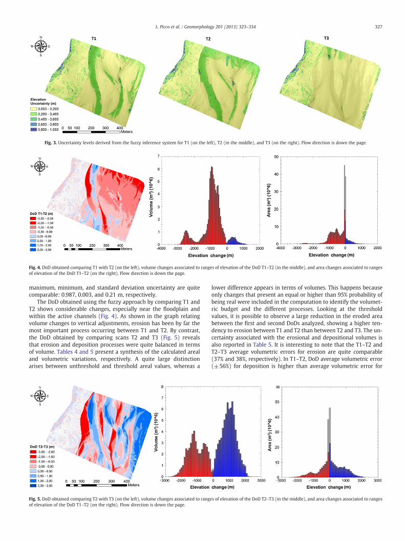
Fig. 3. Uncertainty levels derived from the fuzzy inference system for T1 (on the left), T2 (in the middle), and T3 (on the right). Flow direction is down the page.

Fig. 4. DoD obtained comparing T1 with T2 (on the left), volume changes associated to ranges of elevation of the DoD T1–T2 (in the middle), and area changes associated to rangesof elevation of the DoD T1–T2 (on the right). Flow direction is down the page.

327L. Picco et al. / Geomorphology 201 (2013) 323–334

maximum, minimum, and standard deviation uncertainty are quitecomparable: 0.987, 0.003, and 0.21 m, respectively.

The DoD obtained using the fuzzy approach by comparing T1 andT2 shows considerable changes, especially near the floodplain andwithin the active channels (Fig. 4). As shown in the graph relatingvolume changes to vertical adjustments, erosion has been by far themost important process occurring between T1 and T2. By contrast,the DoD obtained by comparing scans T2 and T3 (Fig. 5) revealsthat erosion and deposition processes were quite balanced in termsof volume. Tables 4 and 5 present a synthesis of the calculated arealand volumetric variations, respectively. A quite large distinctionarises between unthreshold and threshold areal values, whereas a

Fig. 5. DoD obtained comparing T2 with T3 (on the left), volume changes associated to rangof elevation of the DoD T1–T2 (on the right). Flow direction is down the page.

lower difference appears in terms of volumes. This happens becauseonly changes that present an equal or higher than 95% probability ofbeing real were included in the computation to identify the volumet-ric budget and the different processes. Looking at the thresholdvalues, it is possible to observe a large reduction in the eroded areabetween the first and second DoDs analyzed, showing a higher ten-dency to erosion between T1 and T2 than between T2 and T3. The un-certainty associated with the erosional and depositional volumes isalso reported in Table 5. It is interesting to note that the T1–T2 andT2–T3 average volumetric errors for erosion are quite comparable(37% and 38%, respectively). In T1–T2, DoD average volumetric error(±56%) for deposition is higher than average volumetric error for

es of elevation of the DoD T2–T3 (in the middle), and area changes associated to ranges

Table 4Summary of areal T1–T2 and T2–T3 DoDs.

T1–T2 T2–T3

Areal Unthresholded Thresholded Unthresholded Thresholded

Total areaof erosion (m2)

193411.97 167143.39 108335.00 85773.74

Total areaof deposition (m2)

60791.25 35263.64 145828.66 121536.35

Fig. 6. Bank erosions registered during the first study period (T1–T2) and the secondone (T2–T3). Flow direction is down the page.

328 L. Picco et al. / Geomorphology 201 (2013) 323–334

erosion (±37%), likely depending on the fact that most of the deposi-tion occurred along the submerged areas that present the lower den-sity and the higher uncertainty. The opposite occurred during thesecond study period with 38% average volumetric error of erosionand 18% average volumetric error of deposition. In this case, the ab-sence of submerged areas during the T3 survey allowed us to collectdata with higher density and, subsequently, to obtain a lower uncer-tainty all over the study area.

4.2. Morphological changes

Analyzing in detail the study area, it clearly appears that consider-able erosion experienced by the right bank of the main channel is def-initely the most relevant morphological change that occurred duringthe study period in the subreach analyzed. In order to investigate indetail the erosion process between the surveys, budget segregationswere carried out on the basis of the obtained DoDs. Using this ap-proach we were able to define the extent and the volume of bank ero-sion, along with the sedimentation processes occurring on the gravel.The bank erosion areas were defined taking into consideration thefloodplain extension in the three DEMs (Fig. 6). The gravel bar areaswere defined by subtraction. During the first study period, therewas a predominant erosion phase (Figs. 7, 8). Along the analyzedbank, there was a total erosion of over 5630 m2 that produced anerosion volume of about 12,214 m3, resulting in a retreat rate of2.17 m3/m2. On the other side, along the gravel bar area, there wasa dominant erosional process over a surface of 144,232 m2 that pro-duced an erosion volume of about 85,473 m3 (rate 0.59 m3/m2).Over the gravel bar, some areas experienced deposition as well(23,746 m2; 6843 m3; deposition rate of about 0.29 m3/m2). Thesegregation analysis allowed us to observe that the bank erosion pro-cesses were deeper than the gravel bar ones, with maximum valuesof −3 m and −2 m respectively. It is also interesting to note asmost of the erosional and depositional processes along the gravelbars happened in areas at elevation between −1 and +1 m,respectively.

Focusing on the second study period (Figs. 9, 10), a further rele-vant bank erosion appears to have happened along a bigger area(10,723 m2) that produced a bigger erosion of about 14,885 m3,resulting in a lower erosion rate of 1.39 m3/m2. As to the changes ex-perienced by the gravel bars during the second period, depositionalprocesses characterized 105,976 m2, whereas erosional processesonly 63,465 m2. Looking at the volumetric changes, it appears thatdeposition dominates over erosion (74,168 vs. 32,136 m3). It is alsointeresting to see as, in this case, the bank erosion reached lowerdepths (−2 m) than during the first study period (−3 m).

Table 5Summary of volumetric T1–T2 and T2–T3 DoDs.

T1–T2

Volumetric Unthresholded Thresholded ±

Total volume of erosion (m3) 98175.98 97990.66 3Total volume of deposition (m3) 6956.48 6863.10Total volume of difference (m3) 105132.46 104853.76 3Total net volume difference (m3) −91219.51 −91127.56 3

4.3. Roughness distribution and variation

A substantial change in the roughness distribution occurred fromT1 to T2 (Fig. 11). This is likely due to the fact that there was a migra-tion of the main channel downstream on the right side of the area,near the right bank. It is interesting to observe that in the upperpart of the study area, just upstream of the secondary channel onthe left, there was a particularly rough area that was maintainedfrom T1 to T2. Looking at the T3 (Fig. 11), it appears that an increaseof roughness occurred over the left part of the study area. In fact, weobserve a large area in the middle upstream and in the left down-stream with high roughness.

Fig. 12 shows the changes in surface roughness during the two studyperiods. It appears that during the first period (T1 to T2) there were notconsistent variations in roughness with the exception of the most rightdownstream area, where there was a widespread increase of about0.44 m maximum. On the other hand, during the period between T2and T3 (Fig. 12), there was a consistent change of roughness. Alongthe central high bars there was an extended increase in roughness aswell as along the left side of the study area (Fig. 12). Conversely towhat happened during the first period, the right downstream portionof the area experienced a consistent decrease in the roughness.

Analyzing in detail the roughness distribution in T1, eight elevationranges (Fig. 13) were defined. Elevations lower than 2 m correspond towet areas (Fig. 13). The lower level has a very limited extension, theothers have variable extension from about 6000 m2 (0.5–1 m) and56,854 m2 (2–2.5 m). Fig. 14 shows that the roughness increases athigher topographical elevations and that areas higher than 3.5 m(with respect to the thalweg) are characterized by a very high rough-ness (around 0.085 m). As in T1, in T2 (Fig. 13) surfaces lying lowerthan 2 m refers to wetted areas. Fig. 14 shows that roughness is muchhigher at high elevations (3.5–4 m) than in T1. In T3 (Fig. 13) eight el-evation ranges were defined too, and also the higher and lower classes

T2–T3

Error volume Unthresholded Thresholded ±Error volume

5946.65 48331.73 48024.99 18403.883852.61 75999.93 75578.61 13672.759799.27 124331.66 123603.60 32076.636152.52 27668.20 27553.62 22926.99

Fig. 7. Bank erosion process, volume (on the left) and area (on the right) between the T1–T2 data acquisition.

329L. Picco et al. / Geomorphology 201 (2013) 323–334

have an area of N10 m2 and the maximum area is on the 2–2.5 m class,with about 64,240 m2. Fig. 14 shows that there are similar mean valuesall over the classes; less for the upper level where the mean value ishigher than the others but significantly lower than the T1 and T2 values.

Fig. 15 shows the correlation between the median roughness, cor-responding to the T2 and T3 surveys and the maximum water stageregistered during the first and second study periods, respectively.A clear difference appears looking at the minimum water depthlevel. In fact, water depths lower than 1 m correspond to the maxi-mum values of median roughness in T2 and T3, about 0.13 and0.05 m, respectively.

5. Discussion

The TLS provides a large amount of detailed surface elevationpoints. However, the main issue related to its use in fluvial systemsis the relatively low point density obtained on the wetted areas. Infact, as shown by Milan et al. (2007), the elevations of the wettedareas surveyed by TLS are affected by significant errors. Cavalli andTarolli (2011) and Lollino et al. (2008) showed that in some cases

Fig. 8. Gravel-bar processes, volume (on the left) and are

the use of bathymetric LiDAR or sonar could solve the issue, andthey work better than optical bathymetric mapping (sensu Williamset al., 2011). In this study, a few points were collected in the sub-merged areas using a dGPS in order to complete the survey. Thelower point density in the wetted areas implies a higher level of un-certainty along the water stage lines, as shown by Fig. 3; but it isworth noticing, as also shown by James et al. (2012), that the DoDmethod is the best suited where changes are greater than uncertainty,which is definitely the case in this study.

In this paper, an ad hoc fuzzy inference system (FIS) to estimateDTM error was developed using point density, slope, and roughnessas the main variables for DTM uncertainty estimation. From a meth-odological point of view, using an index of roughness directly deriv-able from a DTM as input for the FIS represents an innovativeapproach that helps to better quantify DTM error connected to localmorphological conditions. This novel approach permits us to definethe spatial variability of uncertainty with higher detail than whatwas presented by Heritage et al. (2009) and Milan et al. (2011),which defined the uncertainty variability based upon using the surfaceroughness and not the grain roughness. The methodology proposed

a (on the right) between the T1–T2 data acquisition.

Fig. 9. Bank erosion process, volume (on the left) and area (on the right) between the T2–T3 data acquisition.

330 L. Picco et al. / Geomorphology 201 (2013) 323–334

here is also an advance onwhatwas proposed byWheaton et al. (2013),in fact the authors used only the point density as proxy for completenessof sampling covered and the slope as proxy for the topographiccomplexity.

The FIS analysis allowed us to assess in detail the morphologicalchanges that occurred in the study area over two subsequents rela-tively short intervals. During the first interval (T1–T2), there was adominant erosional tendency (−91,127 m3), whereas during the sec-ond one (T2–T3) the study reach experienced a slight aggradation(27,553 m3). The two periods are characterized by different durationsand flood types. The interval T1–T2 lasted two months during latesummer and featured three flood pulses with flow stage measuredat Villuzza higher than 1.6 m, thus slightly lower than the 1-yearrecurrence interval. Summer flood pulses are typically generated bylocalized convective cells and are thus relatively flashy, lastingb6 days. On the same study reach, Bertoldi et al. (2010) showedthat relatively short-lasting flood pulses can lead to relevant morpho-logical changes. On the other side, the interval T2–T3 lasted 10 monthsand featured five flood events, peaking higher than 1.6 m. Two of thesefloods were well above the bankfull stage, lasted longer than 20 days,

Fig. 10. Gravel bar processes, volume (on the left) and are

and were generated by long-lasting precipitations typical of the winterperiod in the study basin. Overall, the results suggest that few short andlow magnitude summer floods were very effective in eroding the bank(2.17 m3/m2) and lowering the level of the bars. Accordingly, Bertoldi etal. (2010) demonstrated, by using digital image acquisition and topo-graphic surveys, that flow pulses are mainly responsible for bank ero-sion. On the contrary, winter and snowmelt floods (characterized bymore numerous and higher floods) eroded the bank at a lower rate(1.39 m3/m2) and deposited sediments in the lower bars. This wouldsuggest that flashy floods generated by concentrated rainfalls in smallportions of the basin are likely to carry a reduced sediment load, leadingthese floods to be very effective in eroding sediments from the studyreach, whereas long-lasting winter floods are more likely to activatesediment sources at the basin scale and to deposit sediments in thestudy reach. Again, this would be supported by Bertoldi et al. (2010),who observed that higher and longer floods are able to activate sedi-ment sources over larger areas.

Regarding the bed surface roughness, itsmaximum value is attainedat the highest elevations, i.e., especially in the high bars. Even if notcurrently supported by numerous field surveys, grain size analysis

a (on the right) between the T2–T3 data acquisition.

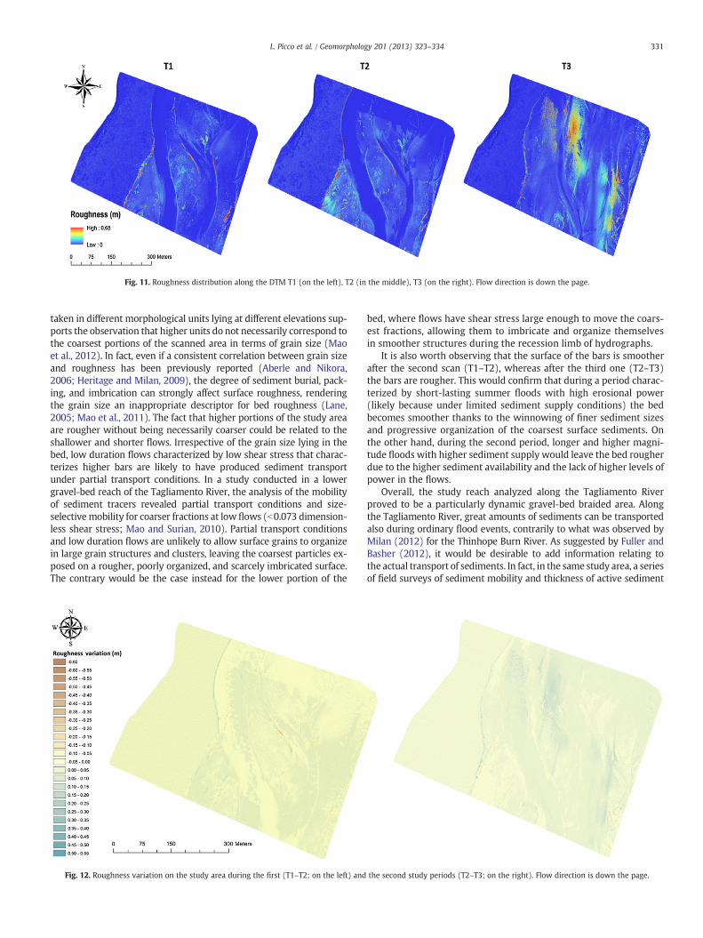
Fig. 11. Roughness distribution along the DTM T1 (on the left), T2 (in the middle), T3 (on the right). Flow direction is down the page.

331L. Picco et al. / Geomorphology 201 (2013) 323–334

taken in different morphological units lying at different elevations sup-ports the observation that higher units do not necessarily correspond tothe coarsest portions of the scanned area in terms of grain size (Maoet al., 2012). In fact, even if a consistent correlation between grain sizeand roughness has been previously reported (Aberle and Nikora,2006; Heritage and Milan, 2009), the degree of sediment burial, pack-ing, and imbrication can strongly affect surface roughness, renderingthe grain size an inappropriate descriptor for bed roughness (Lane,2005; Mao et al., 2011). The fact that higher portions of the study areaare rougher without being necessarily coarser could be related to theshallower and shorter flows. Irrespective of the grain size lying in thebed, low duration flows characterized by low shear stress that charac-terizes higher bars are likely to have produced sediment transportunder partial transport conditions. In a study conducted in a lowergravel-bed reach of the Tagliamento River, the analysis of the mobilityof sediment tracers revealed partial transport conditions and size-selective mobility for coarser fractions at low flows (b0.073 dimension-less shear stress; Mao and Surian, 2010). Partial transport conditionsand low duration flows are unlikely to allow surface grains to organizein large grain structures and clusters, leaving the coarsest particles ex-posed on a rougher, poorly organized, and scarcely imbricated surface.The contrary would be the case instead for the lower portion of the

Fig. 12. Roughness variation on the study area during the first (T1–T2; on the left) and

bed, where flows have shear stress large enough to move the coars-est fractions, allowing them to imbricate and organize themselvesin smoother structures during the recession limb of hydrographs.

It is also worth observing that the surface of the bars is smootherafter the second scan (T1–T2), whereas after the third one (T2–T3)the bars are rougher. This would confirm that during a period charac-terized by short-lasting summer floods with high erosional power(likely because under limited sediment supply conditions) the bedbecomes smoother thanks to the winnowing of finer sediment sizesand progressive organization of the coarsest surface sediments. Onthe other hand, during the second period, longer and higher magni-tude floods with higher sediment supply would leave the bed rougherdue to the higher sediment availability and the lack of higher levels ofpower in the flows.

Overall, the study reach analyzed along the Tagliamento Riverproved to be a particularly dynamic gravel-bed braided area. Alongthe Tagliamento River, great amounts of sediments can be transportedalso during ordinary flood events, contrarily to what was observed byMilan (2012) for the Thinhope Burn River. As suggested by Fuller andBasher (2012), it would be desirable to add information relating tothe actual transport of sediments. In fact, in the same study area, a seriesof field surveys of sediment mobility and thickness of active sediment

the second study periods (T2–T3; on the right). Flow direction is down the page.

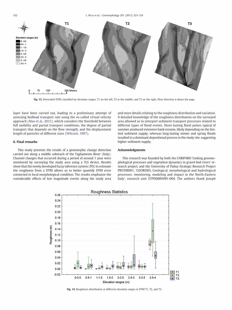
Fig. 13. Detrended DTM, classified by elevation ranges, T1 on the left, T2 in the middle, and T3 on the right. Flow direction is down the page.

332 L. Picco et al. / Geomorphology 201 (2013) 323–334

layer have been carried out, leading to a preliminary attempt ofassessing bedload transport rate using the so-called virtual velocityapproach (Mao et al., 2012), which considers the threshold betweenfull mobility and partial transport conditions, the degree of partialtransport that depends on the flow strength, and the displacementlength of particles of different sizes (Wilcock, 1997).

6. Final remarks

This study presents the results of a geomorphic change detectioncarried out along a middle subreach of the Tagliamento River (Italy).Channel changes that occurred during a period of around 1 year weremonitored by surveying the study area using a TLS device. Resultsshow that the newly developed fuzzy inference system (FIS) to estimatethe roughness from a DTM allows us to better quantify DTM errorconnected to local morphological condition. The results emphasize theconsiderable effects of low magnitude events along the study area

Fig. 14. Roughness distribution at different

andmore details relating to the roughness distribution and variation.A detailed knowledge of the roughness distribution on the surveyedarea allowed us to interpret sediment transport processes related todifferent types of flood events. Short-lasting flood pulses typical ofsummer produced extensive bank erosion, likely depending on the lim-ited sediment supply, whereas long-lasting winter and spring floodsresulted in a dominant depositional process in the study site, suggestinghigher sediment supply.

Acknowledgments

This research was founded by both the CARIPARO ‘Linking geomor-phological processes and vegetation dynamics in gravel-bed rivers’ re-search project, and the University of Padua Strategic Research ProjectPRST08001, ‘GEORISKS, Geological, morphological and hydrologicalprocesses: monitoring, modeling and impact in the North-EasternItaly’, research unit STPD08RWBY-004. The authors thank Joseph

elevation ranges in DTM T1, T2, and T3.

0

0.04

0.08

0.12

0.16

0 1 2 3 4 5

Water depth (m)

Ro

ug

hn

ess

(m)

T2

T3

Fig. 15. Median roughness value of T2 and T3 related to the maximum water depthbetween T1 and T2 and between T2 and T3.

333L. Picco et al. / Geomorphology 201 (2013) 323–334

M. Wheaton and an anonymous referee for providing critical com-ments that greatly improved the clarity and accuracy of the paper.

References

Aberle, J., Nikora, V., 2006. Statistical properties of armored gravel-bed surfaces. WaterResources Research 42, W11414. http://dx.doi.org/10.1029/2005WR004674.

Ashmore, P.E., 1991. How do gravel-bed rivers braid? Canadian Journal of Earth Sciences28 (3), 326–341. http://dx.doi.org/10.1139/e91-030.

Ashmore, P.E., Varkaris, F., Chandler, J., Stojic, M., Luce, J., 2000. Animation of a se-quence of DEMs of a braided river physical model. Gravel Bed Rivers V, CD ROM.New Zealand Hydrological Society, Wellington, New Zealand.

Ashworth, P.J., Ferguson, R.I., 1986. Interrelationships of channel processes, changesand sediments in a proglacial braided river. Geografiska Annaler 68A, 361–371.

Ashworth, P.J., Ferguson, R.I., Ashmore, P.E., Paola, C., Powell, D.M., Prestegaard, K.L., 1992.Measurements in a braided river chute and lobe: 2. Sorting of bed loadduring entrain-ment, transport, and deposition. Water Resources Research 28, 1887–1896.

Bertoldi, W., Zanoni, L., Tubino, M., 2009. Planform dynamics of braided streams. EarthSurface Processes and Landforms 34, 547–557. http://dx.doi.org/10.1002/esp.1755.

Bertoldi, W., Zanoni, L., Tubino, M., 2010. Assessment of morphological changes inducedby flow and flood pulses in a gravel bed braided river: the Tagliamento River (Italy).Geomorphology 114, 348–360. http://dx.doi.org/10.1016/j.geomorph.2009.07.017.

Brasington, J., Rumsby, B.T., McVey, R.A., 2000. Monitoring and modelling morpholog-ical change in a braided gravel-bed river using high resolution GPS-based survey.Earth Surface Processes and Landforms 25, 973–990. http://dx.doi.org/10.1002/1096-9837(200008)25:9b973::AID-ESP111N3.0.CO;2-Y.

Brasington, J., Langham, J., Rumsby, B., 2003. Methodological sensitivity of morphomet-ric estimates of coarse fluvial sediment transport. Geomorphology 53, 299–316.http://dx.doi.org/10.1016/S0169-555X(02)00320-3.

Brierley, G., Fryirs, K., 2005. Geomorphology and River Management: Applications ofthe River Styles Framework. Blackwell Publishing, Victoria, Australia (398 pp.).

Cavalli, M., Marchi, L., 2008. Characterization of the surface morphology of an alpinealluvial fan using airborne LiDAR. Natural Hazards and Earth System Sciences 8,323–333.

Cavalli, M., Tarolli, P., 2011. Application of LiDAR technology for rivers analysis. ItalianJournal of Engineering Geology and Environment, Special Issue 1. http://dx.doi.org/10.4408/IJEGE.20.

Cavalli, M., Tarolli, P., Marchi, L., Dalla Fontana, G., 2008. The effectiveness of airborneLiDAR data in the recognition of channel-bed morphology. Catena 73 (3), 249–260.http://dx.doi.org/10.1016/j.catena.2007.11.001.

Cavalli, M., Trevisani, S., Comiti, F., Marchi, L., 2013. Geomorphometric assessment ofspatial sediment connectivity in small alpine catchments. Geomorphology 188,31–41. http://dx.doi.org/10.1016/j.geomorph.2012.05.007.

Charlton, M.E., Large, A.R.G., Fuller, I.C., 2003. Application of airborne LiDAR in riverenvironments: the river Coquet, Northumberland, UK. Earth Surface Processesand Landforms 28, 299–306. http://dx.doi.org/10.1002/esp.482.

Church, M., Ashmore, P., 1998. Sediment transport and river morphology: a paradigmfor study. In: Klingeman, P.C. (Ed.), Gravel-Bed Rivers in the Environment. WaterResources Center, Highlands Ranch, CO.

Ferguson, R.I., 1993. Understanding braiding process in gravel-bed rivers: progress andunresolved problems. In: Best, J.L., Bristow, C.S. (Eds.), Braided Rivers, Geological SocietySpecial Publication75.Geological Society, Bath, UK, pp. 73–87. http://dx.doi.org/10.1144/GSL.SP.1993.075.01.03.

Ferguson, R.I., Ashmore, P.E., Ashworth, P.J., Paola, C., Prestegaard, K.L., 1992. Measure-ments in a braided river chute and lobe, 1. Flow pattern, sediment transport, andchannel change. Water Resources Research 28 (7), 1877–1886. http://dx.doi.org/10.1029/92WR00700.

French, J.R., 2003. Airborne LiDAR in support of geomorphological and hydraulicmodelling. Earth Surface Processes and Landforms 28, 321–335. http://dx.doi.org/10.1002/esp.484.

Fuller, I.C., Basher, L.R., 2012. Riverbed digital elevation models as a tool for holisticrivermanagement:Motueka River, Nelson, NewZealand. River Research and Applica-tions. http://dx.doi.org/10.1002/rra.2555.

Fuller, I.C., Large, A.R.G., Milan, D.J., 2003. Quantifying development and sedimenttransfer following chute cutoff in a wandering gravel-bed river. Geomorphology54, 307–323. http://dx.doi.org/10.1016/S0169-555X(02)00374-4.

Fuller, I.C., Large, A.R.G., Heritage, G.L., Milan, D.J., Charlton, M.E., 2009. Derivation ofannual reach-scale sediment transfers in the River Coquet, Northumberland, UK.In: Blum, M.D., Marriott, S.B., Leclair, S.F. (Eds.), Fluvial Sedimentology VII. Black-well Publishing Ltd., Oxford, UK. http://dx.doi.org/10.1002/9781444304350.ch4.

Grohmann, C.H., Smith, M.J., Riccomini, C., 2011. Multiscale analysis of topographic sur-face roughness in the Midland Valley, Scotland. IEEE Transactions on Geoscienceand Remote Sensing 49 (4), 1200–1213.

Hancock, G.R., 2006. The impact of different gridding methods on catchment geomor-phology and soil erosion over long timescales using a landscape evolution model.Earth Surface Processes and Landforms 31, 1035–1050.

Heritage, G., Hetherington, D., 2007. Towards a protocol for laser scanning in fluvialgeomorphology. Earth Surface Processes and Landforms 32, 66–74. http://dx.doi.org/10.1002/esp.1375.

Heritage, G.L., Milan, D.J., 2009. Terrestrial laser scanning of grain roughness in agravel-bed river. Geomorphology 113, 4–11. http://dx.doi.org/10.1016/j.geomorph.2009.03.021.

Heritage, G.L., Fuller, I.C., Charlton,M.E., Brewer, P.A., Passmore, D.P., 1998. CDWphotogram-metry of low relief fluvial features: accuracy and implications for reach-scale sedimentbudgeting. Earth Surface Processes and Landforms 23, 1219–1233. http://dx.doi.org/10.1002/(SICI)1096-9837(199812)23:13b1219::AID-ESP927N3.0.CO;2-R.

Heritage, G.L.,Milan,D.J., Large, A.R.G., Fuller, I., 2009. Influenceof survey strategy and inter-polation model upon DEM quality. Geomorphology 112, 334–344. http://dx.doi.org/10.1016/j.geomorph.2009.06.024.

Hicks, D.M., Duncan, M.J., Lane, S.T., Tal, M., Westway, R., 2007. Contemporary morpho-logical change in braided gravel-bed river: new developments from field and lab-oratory studies, with particular reference to the influence of riparian vegetation.In: Habersack, H., Piegay, H., Rinaldi, M. (Eds.), Gravel Bed Rivers VI: From Process-es Understanding to River Restoration. Elsevier, St. Jakob, Austria, pp. 557–584.http://dx.doi.org/10.1016/s0928-2025(07)11143-3.

Höfle, B., Vetter, M., Pfeifer, N., Mandlburger, G., Stötter, J., 2009. Water surface map-ping from airborne laser scanning using signal intensity and elevation data. EarthSurface Processes and Landforms 34 (12), 1635–1649. http://dx.doi.org/10.1002/esp.1853.

Horn, B.K.P., 1981. Hill shading and the reflectance map. Proceedings of the Institutionof Electrical Engineers 69, 14–47.

James, L.A., Hodgson, M.E., Ghoshal, S., Latiolais, M.M., 2012. Geomorphic change de-tection using historic maps and DEM differencing: the temporal dimension ofgeospatial analysis. Geomorphology 137, 181–198. http://dx.doi.org/10.1016/j.geomorph.2010.10.039.

Lane, S.N., 1998. The use of digital terrain modeling in the understanding of dynamicriver system. In: Lane, S.N., Richards, K.S., Chandler, J.H. (Eds.), LandformMonitoring,Modelling and Analysis. Wiley, Chichester, UK, pp. 311–342.

Lane, S.N., 2005. Roughness — time for a re‐evaluation? Earth Surface Processes andLandforms 30 (2), 251–253. http://dx.doi.org/10.1002/esp.1208.

Lane, S.N., Chandler, J.H., 2003. The generation of high quality topographic data forhydrology and geomorphology: new data sources, new applications and new prob-lems. Earth Surface Processes and Landforms 28 (3), 229–230. http://dx.doi.org/10.1002/esp.479.

Lane, S.N., Richards, K.S., 1998. High resolution, two-dimensional spatialmodelling offlowprocesses in a multi-thread channel. Hydrological Processes 12, 1279–1298. http://dx.doi.org/10.1002/(SICI)1099-1085(19980630)12:8b1279::AID-HYP615N3.0.CO;2-E.

Lane, S.N., Chandler, J.H., Richards, K.S., 1994. Developments in monitoring and terrainmodelling small-scale river-bed topography. Earth Surface Processes and Landforms19, 349–368. http://dx.doi.org/10.1002/esp.3290190406.

Lane, S.N., Westaway, R.M., Hicks, D.M., 2003. Estimation of erosion and depositionvolumes in a large, gravel-bed, braided river using synoptic remote sensing.Earth Surface Processes and Landforms 28, 249–271. http://dx.doi.org/10.1002/esp.483.

Leopold, L.B., Wolman, M.G., 1957. River channel patterns: braided, meandering andstraight. U.S. Geological Survey Professional Papers 282B, 39–85.

Lindsay, J.B., Ashmore, P.E., 2002. The effects of survey frequency on estimates of scourand fill in a braided river model. Earth Surface Processes and Landforms 27, 27–43.http://dx.doi.org/10.1002/esp.282.

Lippert, W., Müeller, N., Rossel, S., Schauer, T., Vetter, G., 1995. Der Tagliamento—Flussmorphologie und Auenvegetation der groessten Wildflusslandschaft in derAlpen. Jahrbuch des Vereins zum Schutz der Bergwelt 60, 11–70.

Lisle, T.E., Nelson, J.M., Pitlick, J., Madej, M.A., Barkett, B.L., 2000. Variability of bedmobilityin natural, gravel-bed channels and adjustments to sediment load at local and reachscales. Water Resources Research 36 (12), 3743–3755. http://dx.doi.org/10.1029/2000WR900238.

Lollino, G., Giordan, D., Baldo, M., Allasia, P., Pellegrini, F., 2008. L'uso di modelli digitalidel terreno come strumento per lo studio dell'evoluzione morfologica dei corsid'acqua: proposte metodologiche e primi risultati. Il Quaternario, Italian Journalof Quaternary Sciences 21 (1B), 331–342.

Mao, L., Surian, N., 2010. Observations on sediment mobility in a large gravel-bed river.Geomorphology 114, 326–337. http://dx.doi.org/10.1016/j.geomorph.2009.07.015.

334 L. Picco et al. / Geomorphology 201 (2013) 323–334

Mao, L., Cooper, J., Frostick, L., 2011. Grain size and topographical differences betweenstatic and mobile armour layers. Earth Surface Processes and Landforms 36 (10),1321–1334. http://dx.doi.org/10.1002/esp.2156.

Mao, L., Picco, L., Surian, N., Lenzi, M.A., 2012. The extent of partial transport in a widegravel-bed river (Tagliamento River, Italy). IS Rivers Conference, Lyon, France.

Mao, L., Picco, L., Cooper, J., Lenzi, M.A., 2013. How surface grain organization influ-ences the relationship between grain size and roughness in gravel-bed rivers (inpreparation).

Marcus, W.A., Fonstad, M.A., 2008. Optical remote mapping of rivers at sub-meter res-olutions and watershed extents. Earth Surface Processes and Landforms 33, 4–24.http://dx.doi.org/10.1002/esp.

Merz, J.E., Pasternack, G.B., Wheaton, J.M., 2006. Sediment budget for salmonid spawninghabitat rehabilitation in the Mokelumne River. Geomorphology 76 (1–2), 207–228.http://dx.doi.org/10.1016/j.geomorph.2005.11.004.

Milan, D.J., 2012. Geomorphic impact and system recovery following an extreme floodin an upland stream: Thinhope Burn, northern England, UK. Geomorphology 138,319–328. http://dx.doi.org/10.1016/j.geomorph.2011.09.017.

Milan, D.J., Heritage, G.L., Hetherington, D., 2007. Application of a 3D laser scanner in theassessment of erosion and deposition volumes and channel change in a proglacialriver. Earth Surface Processes and Landforms 32, 1657–1674. http://dx.doi.org/10.1002/esp.1592.

Milan, D.J., Heritage, G.L., Large, A.R., Fuller, I.C., 2011. Filtering spatial error from DEMs:implications formorphological change estimation. Geomorphology 125 (1), 160–171.http://dx.doi.org/10.1016/j.geomorph.2010.09.012.

Milne, J.A., Sear, D.A., 1997. Modelling river channel topography using GIS. Interna-tional Journal of Geographical Information Science 11 (5). http://dx.doi.org/10.1080/13658819724227.

Moretto, J., Delai, F., Rigon, E., Picco, L., Mao, L., Lenzi, M.A., 2012. Assessing shortterm erosion-deposition processes of the Brenta River using LiDAR surveys. WITTransactions on Engineering Sciences 73, 149–160. http://dx.doi.org/10.2495/DEB120131 (1743-3553).

Müller, N., 1995. River dynamics and floodplain vegetation and their alteration due tohuman impact. Archiv für Hydrobiologie Supplementband 101, 477–512.

Notebaert, B., Verstraeten, G., Govers, G., Poesen, J., 2009. Qualitative and quantitativeapplications of LiDAR imagery in fluvial geomorphology. Earth Surface Processesand Landforms 34 (2), 217–231. http://dx.doi.org/10.1002/esp.1705.

Picco, L., Mao, L., Rigon, E., Moretto, J., Ravazzolo, D., Delai, F., Lenzi, M.A., 2012a. Mediumterm fluvial island evolution in relation with flood events in the Piave River. WITTransactions on Engineering Sciences 73, 161–172. http://dx.doi.org/10.2495/DEB120141 (1743-3553).

Picco, L., Mao, L., Rigon, E., Moretto, J., Ravazzolo, D., Delai, F., Lenzi, M.A., 2012b.Riparian forest structure, vegetation cover and flood events in the Piave River.WIT Transactions on Engineering Sciences 73, 137–147. http://dx.doi.org/10.2495/DEB120121 (1743-3553).

Rumsby, B.T., Brasington, J., Langham, J.A., McLelland, S.J., Middleton, R., Rollinson, G.,2008. Monitoring and modelling particle and reach-scale morphological changein gravel-bed rivers: applications and challenges. Geomorphology 93 (1-2), 40–54.http://dx.doi.org/10.1016/j.geomorph.2006.12.017.

Tarolli, P., Arrowsmith, J.R., Vivoni, E.R., 2009. Understanding earth surface processesfrom remotely sensed digital terrain models. Geomorphology 113, 1–3.

Thoma, D.P., Gupta, S.C., Bauerc, M.E., Kirchoff, C.E., 2005. Airborne laser scanningfor riverbank erosion assessment. Remote Sensing of Environment 95, 493–501.http://dx.doi.org/10.1016/j.rse.2005.01.012.

Tockner, K., Ward, J.V., Arscott, D.B., 2003. The Tagliamento River: a model ecosystemof European importance. Aquatic Sciences 65, 239–253. http://dx.doi.org/10.1007/s00027-003-0699-9.

Ward, J.V., Tockner, K., Edwards, P.J., Kollmann, J., Bretschko, G., Gurnell, A.M., Petts, G.E.,Rossaro, B., 1999. A reference river system for the Alps: the ‘Fiume Tagliamento’.Regulated Rivers: Research & Management 15, 63–75. http://dx.doi.org/10.1002/(SICI)1099-1646(199901/06)15:1/3b63::AID-RRR538N3.0.CO;2-F.

Wechsler, S.P., 2003. Perceptions of digital elevation model uncertainty by DEM users.URISA Journal 15, 57–64.

Wechsler, S.P., Kroll, C.N., 2006. Quantifying DEM uncertainty and its effect ontopographic parameters. Photogrammetric Engineering and Remote Sensing72, 1081–1090.

Wheaton, J.M., 2008. Uncertainty in Morphological Sediment Budgeting of Rivers.(Ph.D. Thesis) University of Southampton, Southampton, UK (412 pp.).

Wheaton, J.M., Brasington, J., Darby, S.E., Sear, D.A., 2010a. Accounting for uncertainty inDEMs from repeat topographic surveys: improved sediment budgets. Earth SurfaceProcesses and Landforms 35, 136–156. http://dx.doi.org/10.1002/esp.1886.

Wheaton, J.M., Brasington, J., Darby, S.E., Merz, J., Pasternak, G.B., Sear, D.A., Vericat, D.,2010b. Linking geomorphic changes to salmonid habitat at a scale relevant to fish.River Research and Applications 26, 469–486. http://dx.doi.org/10.1002/rra.1305.

Wheaton, J.M., Brasington, J., Darby, S.E., Kasprak, A., Sear, D.A., Vericat, D., 2013.Morphodynamic signatures of braiding mechanisms as expressed throughchange in sediment storage in a gravel-bed river. Journal of Geophysical Re-search. http://dx.doi.org/10.1002/jgrf.20060.

Wilcock, P.R., 1997. Entrainment, displacement and transport of tracer gravels. EarthSurface Processes and Landforms 22, 1125–1138.

Williams, R., Brasington, J., Vericat, D., Hicks, M., Labrossee, F., Neal, M., 2011. Monitoringbraided river change using terrestrial laser scanning and optical bathymetric mapping.Developments in Earth Surface Processes (ISSN: 0928-2025) 15. http://dx.doi.org/10.1016/B978-0-444-53446-0.00020-3.

Wise, S.M., 1998. The effect of GIS interpolation errors on the use of DEMs in geomor-phology. In: Lane, S.N., Richards, K.S., Chandler, J.H. (Eds.), Landform Monitoring,Modelling and Analysis. Wiley, Chichester, UK, pp. 139–164.

Wise, S.M., 2007. Effect of differing DEM creation methods on the results from a hydro-logical model. Computers and Geosciences 33, 1351–1365.