Evaluating salinity distribution in soil irrigated with saline water in arid regions of northwest China

Page 1

Eo

Wa

b

c

a

AA

KISM

1

aiceX2hto2c

wa2iti

0d

Agricultural Water Management 97 (2010) 2001–2008

Contents lists available at ScienceDirect

Agricultural Water Management

journa l homepage: www.e lsev ier .com/ locate /agwat

valuating salinity distribution in soil irrigated with saline water in arid regionsf northwest China

eiping Chena, Zhenan Houb,∗, Laosheng Wuc, Yongchao Liangb, Changzhou Weib

State Key Lab of Urban and Regional Ecology, Research Center for Eco-Environmental Sciences, Chinese Academy of Sciences, Beijing 100085, ChinaDepartment of Resources and Environmental Sciences, Shihezi University, No. 4, North Road, Shihezi, Xinjiang 832003, ChinaDepartment of Environmental Sciences, University of California, Riverside, CA 92521, USA

r t i c l e i n f o

rticle history:vailable online 25 June 2010

eywords:rrigation managementoil salinityodel

a b s t r a c t

In arid and semi-arid regions, salinity is a serious and chronic problem for agriculture. A 3-year fieldexperiment in the arid environment of Xinjiang, northwest China, was conducted to study the salinitychange in soil resulting from deficit irrigation of cotton with non-saline, moderate saline and high salinewater. The salinity profile distribution was also evaluated by an integrated water, salinity, and nitrogenmodel, ENVIRO-GRO. The simulated and observed salinity distributions matched well. Results indicatedthat after 3 years of cotton production, the average salinity in the 1.0-m soil profile was 336% and 547% of

the original soil profile, respectively, for moderate saline and high saline water irrigation. If the practicescontinued, the average soil salinity (ECe) in the 1.0-m soil profile would approach a steady level of 1.7, 10.8,and 14.7 dS m−1, respectively, for the treatments receiving irrigation waters of 0.33, 3.62, and 6.71 dS m−1.It was concluded that deficit irrigation of saline water in this region was not sustainable. Model simulationshowed that a big flood irrigation after harvest can significantly reduce the salt accumulation in the soilprofile, and that this practice was much more efficient for salinity control than applying the same extra

he gr

amount of water during t

. Introduction

In irrigated cropland of semi-arid and arid regions, salinity isserious and chronic problem (van Schilfgaarde, 1994). Salin-

ty impacts about one-third (1.23 × 106 ha) of the total irrigatedropland in Xinjiang, northwest China (Hou et al., 2007). It wasstimated that the salt accumulation in the irrigated croplands ofinjiang was increased by 40% from 1983 to 2005 (Wang et al.,008). In Xinjiang, irrigation water sources are often brackish sinceigh-quality water for agricultural purposes is becoming scare dueo rising demands from urban areas. The salinity level for mostf the shallow groundwater sources in this region is greater thandS m−1. Sustainable crop productivity in these regions is severelyhallenged by the diminishing available water and rising salinity.

The future of irrigated agriculture will need to include the use ofaters containing higher levels of soluble salts, particularly in arid

nd semi-arid regions (Oster and Wichelns, 2003; Malash et al.,

008). The key to saline water irrigation is maintaining the salin-

ty level of the root zone through leaching, which can be achievedhrough flushing excessive soluble salts out of the root zone dur-ng the growing season or additional leaching at the end of the

∗ Corresponding author. Tel.: +86 993 2058076; fax: +86 993 2057990.E-mail address: [email protected] (Z. Hou).

378-3774/$ – see front matter © 2010 Elsevier B.V. All rights reserved.oi:10.1016/j.agwat.2010.03.008

owing season.© 2010 Elsevier B.V. All rights reserved.

season (Corwin et al., 2007). This requires the understanding of theinteractions between irrigation, soil salinity, and crop performance.

The interactions between salinity and plant water uptake arecomplex and affected by many factors. Evaluating the interactionof these factors through field research is difficult and expensivebecause numerous uncontrolled factors may affect crop perfor-mance in addition to the controlled variables. In addition, themagnitude of salt accumulation in a single growth season is oftensmall and may not be readily detectable by the routine soil sam-pling in the field. Simulation models that integrate the effects ofmanagement on crop growth and leaching of chemicals belowthe root zone, on the other hand, provide a means of supple-menting information gained from field experiment (Singh andSingh, 1996). There are numbers of models dealing with plantgrowth, water flow, and agricultural chemical movement, includ-ing GLEAMS (Leonard et al., 1987), LEACHM (Hutson and Wagenet,1992), UNSATCHEM (Simunek et al., 1996), RZWQM (Hanson etal., 1998), SWAGMAN (Khan et al., 2003), and SALTMED (Ragabet al., 2005). Combining with a 3-year field experiment, Forkutsaet al. (2009a,b) applied the soil-water model Hydrus-1D to under-

stand the effects of water management strategies on soil salinityunder cotton irrigated with shallow groundwater. Using an inte-grated water, salinity, and nitrogen model, ENVIRO-GRO, Feng et al.(2003a,b) evaluated effects of irrigation management under salineconditions on plant growth and salt distribution.

Page 2

2002 W. Chen et al. / Agricultural Water Management 97 (2010) 2001–2008

Table 1Chemical characteristics of the three irrigation water.

Water salinity (dS m−1) pH SAR (mmol L−1)1/2 Ion concentration (mmol L−1)

K+ Na+ Ca2+ Mg2+ Cl−

0.3 7.54 – 0.03 – 1.22 0.59 2.45

iDwoetiatmladD

isoo

2

2

iisTwamasrT6dsps1

2

TA

3.6 7.20 7.316.7 7.13 10.4

In Xinjiang, saline water is increasingly used by drip irrigationn cotton (Gossipium hirsutum L.), a highly salinity tolerant plant.rip irrigation is thought to be the most efficient irrigation method,hich can distribute water more uniformly, control the amount

f water application more precisely, and more effectively reducevaporation and deep percolation (Mohammad, 2004). The irriga-ion practice (deficit irrigation with poor quality water) howevers questionable with regard to its long-term sustainability for thegricultural development in Xinjiang where rainfall is insufficiento provide adequate leaching. In the short term, considerable salt

ay be stored in the root zone without causing significant yieldoss. Prolonged deficit irrigation with poor quality water eventu-lly, however, may cause “secondary salinization”, progressivelyecrease yield and compromise the soil resources (Beltran, 1999;udely et al., 2008).

The objective of this research is to evaluate the effect of deficitrrigation in a cotton field applied with different levels of wateralinity under arid climate conditions of Xinjiang on the changef soil salinity based on a 3-year field experiment and simulationutcomes from the revised ENVIRO-GRO model.

. Materials and methods

.1. Field experiment

The field experiments were conducted at an agricultural exper-ment station of Shihezi University, located in Shihezi, Xinjiangn the northwestern China (44◦18′N, 86◦02′E). The region is clas-ified as a warm-temperate arid zone with continental climate.he average annual precipitation is about 170 mm, 60% or more ofhich occurs between April and August. The annual mean temper-

ture is 6.9 ◦C and annual total sunshine is 2770 h. The long-termean maximum and minimum air temperature is 26.1 ◦C in July

nd −18 ◦C in January, respectively. The relative humidity duringummer months varies from 30% to 50%. Annual potential evapo-ation is about 1660 mm. The elevation ranges from 300 to 400 m.he groundwater (generally has a EC of 3–5 dS m−1) table is aboutm from the surface. The study site has a flat topography. The grayesert soils in the study area are of alluvial origin. The soil bulk den-ity varies from 1.27 to 1.45 Mg m−3 in the 1-m soil profile, with a

H range of 7.50–7.88. The average electrical conductivity of theoil saturation extract (ECe) in the soil profile varies from 1.15 to.90 dS m−1.

Cotton (G. hirsutum L., cv. Xinluzao 13) was grown from004 to 2006. The sowing took place in late-April and the har-

able 2mounts of rainfall and irrigation (mm) of the experimental site for the three growing se

Year Potential ETc Amount of rainfall Amount of

Growth season Total April

2004 647 146 190 120a

2005 618 110 149 02006 655 100 149 0

a Amount of non-saline water applied to the saline water irrigation treatments.

0.05 16.4 9.50 0.61 35.50.10 31.8 18.12 0.60 68.1

vest took place around mid-September each year. To reduce thevariability in soil salinity and volumetric water content at thebeginning of the study, 120 mm of fresh water (EC = 0.3 dS m−1)was applied by flood irrigation in 2004. There were threeirrigation water treatments, i.e. non-saline water with EC of0.3 dS m−1, moderate saline water with EC of 3.6 dS m−1, andhigh saline water with EC of 6.7 dS m−1. The saline water wasobtained by adding NaCl and CaCl2 to the non-saline water.The elemental composition of the irrigation waters is shown inTable 1.

The spatial distribution of the experimental plots followed a ran-domized block design. For each irrigation treatment, there were sixreplicates (plots). In each plot, there were two 1.2 m × 25 m beds,with a 0.6-m separation distance. Each bed had four plant rows witha 0.3-m separation distance and was covered with plastic film. Twoirrigation dripper lines were installed under the plastic film. Thecotton plants were sown at 0.1-m intervals in the row to yield apopulation of 222,000 plants ha−1.

The irrigation schemes for the three growing seasons are sum-marized in Table 2. The irrigation schedules were based on the localrecommendations for the non-saline soils of the area. During the3 years of experiment, the applied irrigation water was 375, 345,and 353 mm in 2004, 2005, and 2006, respectively. For all treat-ments, equal volumes of water were irrigated each year. Plots weredrip-irrigated with 30 mm fresh water to improve germination andseedling establishment after sowing in 2005 and 2006. Drip irriga-tion was commenced towards the early June and continued up toAugust during the cotton growing season. The irrigation intervalwas 7–15 days according to field practices used by local farmers.Water meters were used to record the amount of water each plotreceived.

To meet the cotton nutrient requirements, 225 kg N ha−1,105 kg P2O5 ha−1, and 60 kg K2O ha−1 were applied each year. Priorto sowing, triple superphosphate and potassium sulfate wereapplied uniformly as base fertilizers and were mixed well by plow-ing. Urea was applied in five equal splits through the drip irrigationsystem during the cotton growing period. The fertilizer solutionwas stored in a 100-L plastic container and was pumped into theirrigation system.

Salinity distribution along the soil profile was monitored at end

of each crop season and weekly during the 2006 growing season.Soil samples were taken at 0.15 and 0.30 m from the emitter (bothsides) at depths of 0–0.2, 0.2–0.4, 0.4–0.6, 0.6–0.8 and 0.8–1.0 m.Soil salinity was determined by measuring the electrical conduc-tivity (EC) of the saturation extracts with a DDS-308A conductivity

asons.

irrigation water

May June July August Total

0 36 45 + 45 + 45 45 + 36a 37230a 45 + 45 45 + 45 + 45 45 + 45a 34530a 45 + 45 45 + 45 + 38 45 + 30 + 30 353

Page 3

er Management 97 (2010) 2001–2008 2003

mC

2

Lnsapseirwaep2

witt

wcwrGaha

e

A

wrsVg

�

wap

di

wqd

2

s

Table 3Soil hydraulic properties of the five soil layers used in the model simulation.

Soil layer (m)

0–0.2 0.2–0.4 0.4–0.6 0.6–0.8 0.8–1.0

�r (cm3 cm−3) 0.061 0.055 0.051 0.064 0.075�s (cm3 cm−3) 0.43 0.42 0.43 0.41 0.41Ks (cm h−1) 1.24 2.75 2.69 0.70 0.53˛ (cm−1) 0.010 0.020 0.023 0.013 0.009n 1.53 1.53 1.46 1.47 1.50

W. Chen et al. / Agricultural Wat

eter (Shanghai Precision & Scientific Instrument Inc., Shanghai,hina).

.2. Model description

The ENVIRO-GRO model was originally developed by Pang andetey (1998). The model simulates movement of water, salts anditrogen in the root zone and crop growth in response to water,alinity and nitrogen stresses. The model had a better scheme toddress the interactions between salinity, crop water uptake andlant growth. Under stressed conditions resulting from inadequateoil-water content or excessive salinity (N stress was not consid-red in this research), plant growth is reduced, which in turn resultsn reduced ET. A relative plant growth factor (Rf) which equals theelative water uptake (plant growth and water uptake relative tohat would occur under non-stressed conditions) is adopted to

djust the water uptake under stress conditions. When water stressxists in any portion of the root system, water uptake occurs fromortions without water stress (Pang and Letey, 1998; Feng et al.,003a).

In this research, the revised ENVIRO-GRO model was used,hich has more accurate numerical solution and with user-friendly

nput and output data management interfaces. In the revised model,he water flow is modeled by the one-dimension Richard’s equa-ion:

∂�

∂t= ∂

∂z

[K(�)

∂H

∂z

]+ A(z, t) (1)

here � is the volumetric water content of the soil (cm3 waterm−3 soil); H is soil hydraulic head (cm), A(z,t) represents the plantater uptake term (cm3 cm−3 h−1); K(�) represents the unsatu-

ated hydraulic conductivity as a function of � (cm h−1). The vanenuchten (1980) equation is used to describe the soil-water char-cteristic relationship between h and K(h), with h being the matricead. The upper boundary and lower boundary conditions are sets atmospheric boundary condition and free drainage, respectively.

Plant root water uptake (term A in Eq. (1)) is simulated by thempirical equation developed by van Genuchten (1987):

(z, t) = Tp(t)� (z, t)�(h, �) (2)

here Tp(t) is potential transpiration rate (cm h−1); � (z, t) is a plantoot distribution function; and �(h, �) is a crop matric potentialalinity stress function. Root growth is simulated by the classicalerhulst-Pearl logistic function. The additive stress function sug-ested by van Genuchten (1987) is selected, which is given by

(h, �) = 1

1 + [((˛h + �)/�50)]3(3)

here h is soil matric potential, � is soil osmotic potential,= �50/h50 with �50 and h50 being the osmotic head and the matricotential at which transpiration is reduced by 50%, respectively.

Salinity in the water is considered to be conservative, namely, noissolution, precipitation, or plant uptake of salts. Salt movement

s governed by the convection–dispersion equation (CDE):

∂(�Cs)∂t

= ∂

∂z

[Ds(�, �)

∂Cs

∂z− �Cs

](4)

here Cs is the salt concentration, v is the pore water velocity as v =/�, q is water flux, and D is a combined diffusion and hydrodynamicispersion coefficient.

.3. Model parameters

The top 1.0-m soil profile was divided into 5 equal layers. Toet the free drainage condition at the 2-m depth, the bottom 1-

�r is the residual water content; �s is the saturated water content; Ks is the saturatedhydraulic; ˛ is the inverse of the air-entry value or bubbling pressure; n is a pore-sizedistribution index.

m profile used the same soil properties of the 5th layer in thetop 1-m profile. The numerical simulation was conducted usingan incremental depth interval, dz, of 0.01 m. The molecular diffu-sion coefficient for salt was set to 0.02 cm2 h−1, based on Hollins etal. (2000). The longitudinal dispersivity was set to 0.01 m based onGelhar et al. (1985) and Lyman et al. (1992).

The initial matric potential was set to −100 cm in the top 1.0 mand −500 cm in the bottom 1.0 m soil profile. The initial salt distri-bution (ECe) was 2.25, 1.84, 1.79, 2.47 and 3.30 dS m−1, respectively,for the five soil layers downwards. The five parameters defining thesoil-water retentivity are summarized in Table 3. These parameterswere obtained from the agricultural experiment station.

Climatic data were obtained from local weather station andthe reference evapotranspiration (ET0) was calculated based onthe dual approach version of the FAO-56 Penman–Monteith equa-tion (Allen et al., 1998). The crop evapotranspiration (ETc) wasestimated based on the ET0 and the crop coefficients from fieldobservation (Allen et al., 1998). The potential ETc is 647, 618 and655 mm, respectively for the crop year of 2004, 2005 and 2006.Water inputs during the crop season including irrigation and rain-fall are 562, 494 and 492 mm, respectively for the three consecutiveyears (see Table 2).

The plant growth and root development parameters were basedon field observations. The plant reached the full development stageon the 80th day was harvested on the 145th day. A root distributionof 40%, 30%, 20% and 10% root in the 1st, 2nd, 3rd and 4th quarterof the 1.0-m root zone was assumed. The salinity stress threshold(ECe) was set as 7.7 dS m−1, above which it would result in reducedgrowth. The ECe at which growth and transpiration was reducedby 50% was set as 17 dS m−1. These two values were based on Maasand Grattan (1999). The water stress threshold was set as −75 kPa(water content of 0.17 cm3/cm3) and the matric potential at whichtranspiration was reduced by 50% was set to −150 kPa (water con-tent of 0.14 cm3/cm3), based on the research results from Plaut etal. (1996) for cotton irrigated with subsurface drip.

2.4. Statistical analysis

The agreement between the predicted and observed datawas evaluated by Nash–Sutcliffe modeling efficiency (Nash andSutcliffe, 1970), root mean square error and index of agreement(Willmott, 1981). The equation for calculating the Nash–Sutcliffemodeling efficiency (EF) is given as

EF = 1 −∑n

i=1(Oi − Pi)2∑n

i=1(Oi − O)2(5)

The equation for calculating the mean square error (RMSE) is

given as

RMSE =

√√√√ n∑i=1

(Pi − Oi)2

n(6)

Page 4

2004 W. Chen et al. / Agricultural Water Management 97 (2010) 2001–2008

Table 4Irrigation schemes of the four simulation scenarios.

Scenario Amount of irrigation water

May June July August Sep. Total

Default 30a 45 + 45 45 + 45 + 38 45 + 30 + 30 353Scenario #1 30a 62 + 62 62 + 62 + 53 62 + 40 + 40 473Scenario #2 30a 70 + 70 70 + 70 + 58 70 + 46 + 46 473Scenario #3 30a 45 + 45 45 + 45 + 38 45 + 30 + 30 120b 473Scenario #4 30a 45 + 45 45 + 45 + 38 45 + 30 + 30 120c 473

g

I

wOa

aW

2

iocfthoettafl3nata

3

3m

tshauAti

dssi

a Fresh water irrigation.b Flooding fresh water irrigation.c Flooding saline water irrigation (ECW = 3.6 dS m−1).

And the equation for calculating the index of agreement (IA) isiven as

A = 1 −∑n

i=1(Oi − Pi)2∑n

i=1(|Pi − O| + |Oi − O|)2(7)

here Pi is the predicted value corresponding to the observed valuei, and O is the observed mean, P is the predicted mean, O′

i= Oi − O

nd P ′i= Pi − P.

In addition, ANOVA analysis was conducted to test the vari-nce among the data obtained from the field by using the SAS forindows (version 9.0, SAS Institute Inc.) software package.

.5. Simulation scenarios

The outcomes of computer models are useful to answer “whatf” types of questions. Starting with a reference scenario, the worstr best possible cases may be illustrated. To demonstrate the effi-iency of the model developed in this manuscript, we designedour additional simulation scenarios including increasing irriga-ion water in the growing season or flooding irrigation after croparvest to study the effect of different irrigation managementsn salt distribution in the soil profile (Table 4). The default (ref-rence) simulation was based on the moderate saline irrigationreatment in this study. For scenarios 1 and 2, the amount of irriga-ion during the crop season was increased from 353 to 473 mmnd to 530 mm, respectively. For scenarios 3 and 4, a 120-mmooding irrigation was applied after crop harvesting. For scenario, fresh water (ECW = 0.3 dS m−1) was used for flooding. For sce-ario 4, saline water (ECW = 3.6 dS m−1) was used for flooding. Thebove described scenarios were conducted by varying the men-ioned parameters while holding the values of the other parameterst the default levels.

. Results and discussion

.1. Temporal and profile distribution of salts: fieldeasurements vs. model predictions

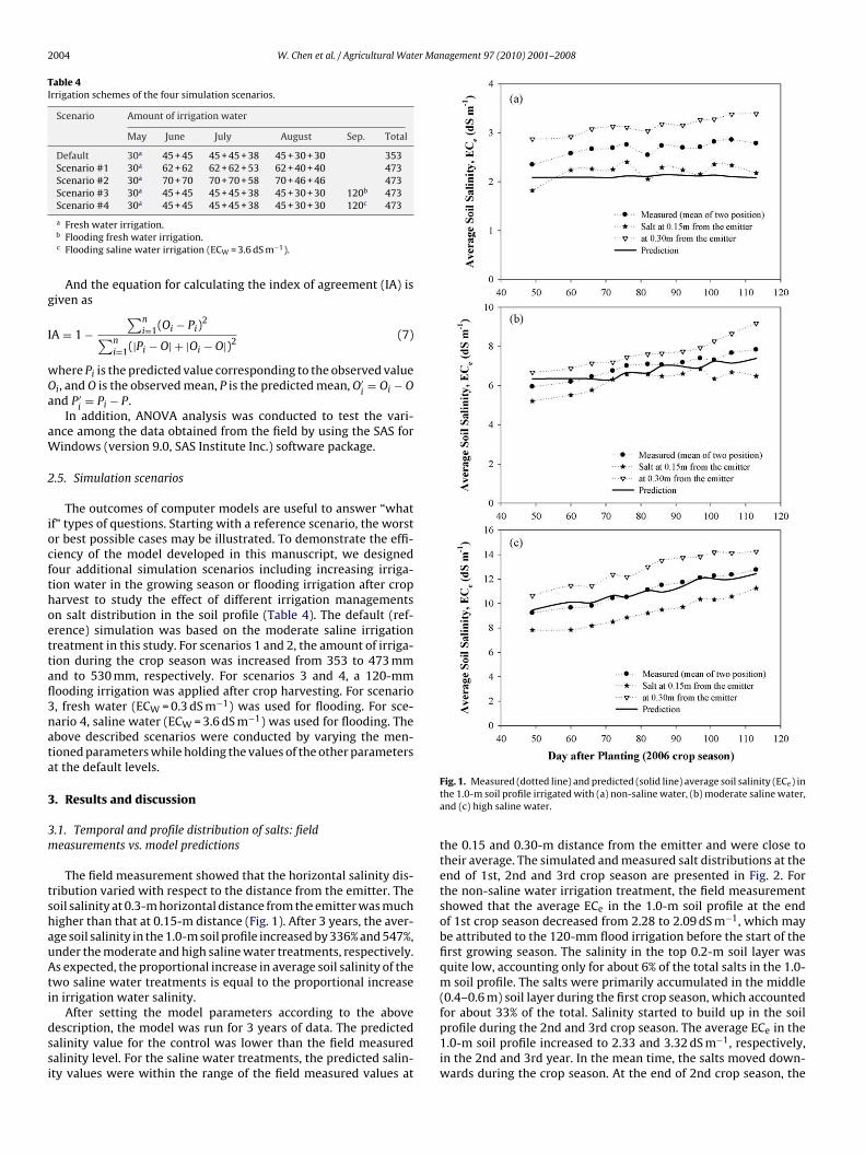
The field measurement showed that the horizontal salinity dis-ribution varied with respect to the distance from the emitter. Theoil salinity at 0.3-m horizontal distance from the emitter was muchigher than that at 0.15-m distance (Fig. 1). After 3 years, the aver-ge soil salinity in the 1.0-m soil profile increased by 336% and 547%,nder the moderate and high saline water treatments, respectively.s expected, the proportional increase in average soil salinity of the

wo saline water treatments is equal to the proportional increasen irrigation water salinity.

After setting the model parameters according to the aboveescription, the model was run for 3 years of data. The predictedalinity value for the control was lower than the field measuredalinity level. For the saline water treatments, the predicted salin-ty values were within the range of the field measured values at

Fig. 1. Measured (dotted line) and predicted (solid line) average soil salinity (ECe) inthe 1.0-m soil profile irrigated with (a) non-saline water, (b) moderate saline water,and (c) high saline water.

the 0.15 and 0.30-m distance from the emitter and were close totheir average. The simulated and measured salt distributions at theend of 1st, 2nd and 3rd crop season are presented in Fig. 2. Forthe non-saline water irrigation treatment, the field measurementshowed that the average ECe in the 1.0-m soil profile at the endof 1st crop season decreased from 2.28 to 2.09 dS m−1, which maybe attributed to the 120-mm flood irrigation before the start of thefirst growing season. The salinity in the top 0.2-m soil layer wasquite low, accounting only for about 6% of the total salts in the 1.0-m soil profile. The salts were primarily accumulated in the middle(0.4–0.6 m) soil layer during the first crop season, which accountedfor about 33% of the total. Salinity started to build up in the soil

profile during the 2nd and 3rd crop season. The average ECe in the1.0-m soil profile increased to 2.33 and 3.32 dS m−1, respectively,in the 2nd and 3rd year. In the mean time, the salts moved down-wards during the crop season. At the end of 2nd crop season, the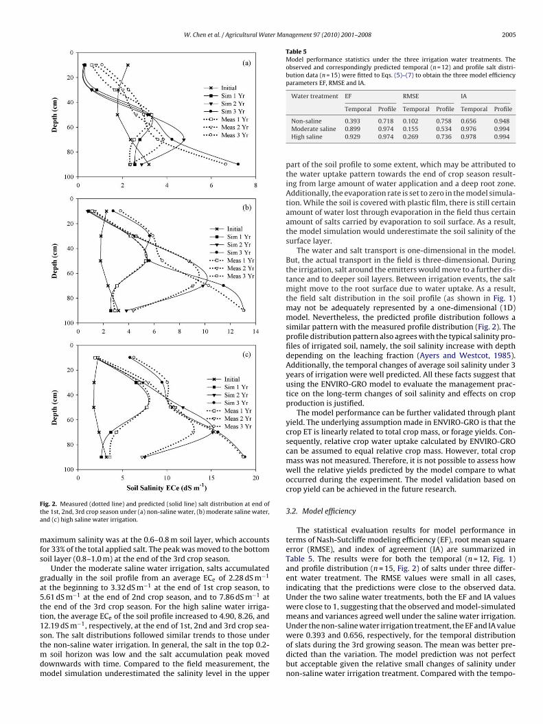

Page 5

W. Chen et al. / Agricultural Water Management 97 (2010) 2001–2008 2005

Fta

mfs

ga5tt1stmdm

Table 5Model performance statistics under the three irrigation water treatments. Theobserved and correspondingly predicted temporal (n = 12) and profile salt distri-bution data (n = 15) were fitted to Eqs. (5)–(7) to obtain the three model efficiencyparameters EF, RMSE and IA.

Water treatment EF RMSE IA

Temporal Profile Temporal Profile Temporal Profile

ig. 2. Measured (dotted line) and predicted (solid line) salt distribution at end ofhe 1st, 2nd, 3rd crop season under (a) non-saline water, (b) moderate saline water,nd (c) high saline water irrigation.

aximum salinity was at the 0.6–0.8 m soil layer, which accountsor 33% of the total applied salt. The peak was moved to the bottomoil layer (0.8–1.0 m) at the end of the 3rd crop season.

Under the moderate saline water irrigation, salts accumulatedradually in the soil profile from an average ECe of 2.28 dS m−1

t the beginning to 3.32 dS m−1 at the end of 1st crop season, to.61 dS m−1 at the end of 2nd crop season, and to 7.86 dS m−1 athe end of the 3rd crop season. For the high saline water irriga-ion, the average ECe of the soil profile increased to 4.90, 8.26, and2.19 dS m−1, respectively, at the end of 1st, 2nd and 3rd crop sea-

on. The salt distributions followed similar trends to those underhe non-saline water irrigation. In general, the salt in the top 0.2-

soil horizon was low and the salt accumulation peak movedownwards with time. Compared to the field measurement, theodel simulation underestimated the salinity level in the upper

Non-saline 0.393 0.718 0.102 0.758 0.656 0.948Moderate saline 0.899 0.974 0.155 0.534 0.976 0.994High saline 0.929 0.974 0.269 0.736 0.978 0.994

part of the soil profile to some extent, which may be attributed tothe water uptake pattern towards the end of crop season result-ing from large amount of water application and a deep root zone.Additionally, the evaporation rate is set to zero in the model simula-tion. While the soil is covered with plastic film, there is still certainamount of water lost through evaporation in the field thus certainamount of salts carried by evaporation to soil surface. As a result,the model simulation would underestimate the soil salinity of thesurface layer.

The water and salt transport is one-dimensional in the model.But, the actual transport in the field is three-dimensional. Duringthe irrigation, salt around the emitters would move to a further dis-tance and to deeper soil layers. Between irrigation events, the saltmight move to the root surface due to water uptake. As a result,the field salt distribution in the soil profile (as shown in Fig. 1)may not be adequately represented by a one-dimensional (1D)model. Nevertheless, the predicted profile distribution follows asimilar pattern with the measured profile distribution (Fig. 2). Theprofile distribution pattern also agrees with the typical salinity pro-files of irrigated soil, namely, the soil salinity increase with depthdepending on the leaching fraction (Ayers and Westcot, 1985).Additionally, the temporal changes of average soil salinity under 3years of irrigation were well predicted. All these facts suggest thatusing the ENVIRO-GRO model to evaluate the management prac-tice on the long-term changes of soil salinity and effects on cropproduction is justified.

The model performance can be further validated through plantyield. The underlying assumption made in ENVIRO-GRO is that thecrop ET is linearly related to total crop mass, or forage yields. Con-sequently, relative crop water uptake calculated by ENVIRO-GROcan be assumed to equal relative crop mass. However, total cropmass was not measured. Therefore, it is not possible to assess howwell the relative yields predicted by the model compare to whatoccurred during the experiment. The model validation based oncrop yield can be achieved in the future research.

3.2. Model efficiency

The statistical evaluation results for model performance interms of Nash-Sutcliffe modeling efficiency (EF), root mean squareerror (RMSE), and index of agreement (IA) are summarized inTable 5. The results were for both the temporal (n = 12, Fig. 1)and profile distribution (n = 15, Fig. 2) of salts under three differ-ent water treatment. The RMSE values were small in all cases,indicating that the predictions were close to the observed data.Under the two saline water treatments, both the EF and IA valueswere close to 1, suggesting that the observed and model-simulatedmeans and variances agreed well under the saline water irrigation.Under the non-saline water irrigation treatment, the EF and IA value

were 0.393 and 0.656, respectively, for the temporal distributionof slats during the 3rd growing season. The mean was better pre-dicted than the variation. The model prediction was not perfectbut acceptable given the relative small changes of salinity undernon-saline water irrigation treatment. Compared with the tempo-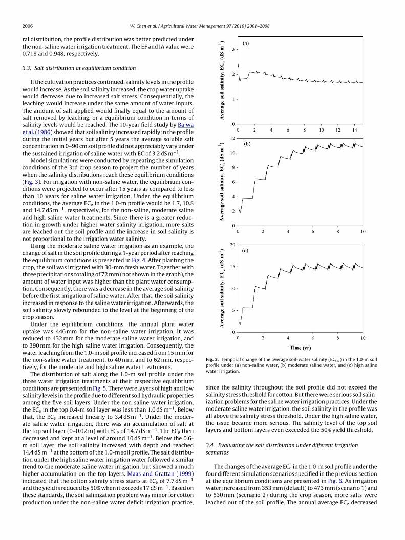

Page 6

2 er Management 97 (2010) 2001–2008

rt0

3

wwlTssedct

cw(dtcaatan

ctctatbisc

urtwtt

tcsattatdm1tthiatp

006 W. Chen et al. / Agricultural Wat

al distribution, the profile distribution was better predicted underhe non-saline water irrigation treatment. The EF and IA value were.718 and 0.948, respectively.

.3. Salt distribution at equilibrium condition

If the cultivation practices continued, salinity levels in the profileould increase. As the soil salinity increased, the crop water uptakeould decrease due to increased salt stress. Consequentially, the

eaching would increase under the same amount of water inputs.he amount of salt applied would finally equal to the amount ofalt removed by leaching, or a equilibrium condition in terms ofalinity levels would be reached. The 10-year field study by Bajwat al. (1986) showed that soil salinity increased rapidly in the profileuring the initial years but after 5 years the average soluble saltoncentration in 0–90 cm soil profile did not appreciably vary underhe sustained irrigation of saline water with EC of 3.2 dS m−1.

Model simulations were conducted by repeating the simulationonditions of the 3rd crop season to project the number of yearshen the salinity distributions reach these equilibrium conditions

Fig. 3). For irrigation with non-saline water, the equilibrium con-itions were projected to occur after 15 years as compared to lesshan 10 years for saline water irrigation. Under the equilibriumonditions, the average ECe in the 1.0-m profile would be 1.7, 10.8nd 14.7 dS m−1, respectively, for the non-saline, moderate salinend high saline water treatments. Since there is a greater reduc-ion in growth under higher water salinity irrigation, more saltsre leached out the soil profile and the increase in soil salinity isot proportional to the irrigation water salinity.

Using the moderate saline water irrigation as an example, thehange of salt in the soil profile during a 1-year period after reachinghe equilibrium conditions is presented in Fig. 4. After planting therop, the soil was irrigated with 30-mm fresh water. Together withhree precipitations totaling of 72 mm (not shown in the graph), themount of water input was higher than the plant water consump-ion. Consequently, there was a decrease in the average soil salinityefore the first irrigation of saline water. After that, the soil salinity

ncreased in response to the saline water irrigation. Afterwards, theoil salinity slowly rebounded to the level at the beginning of therop season.

Under the equilibrium conditions, the annual plant waterptake was 446 mm for the non-saline water irrigation. It waseduced to 432 mm for the moderate saline water irrigation, ando 390 mm for the high saline water irrigation. Consequently, theater leaching from the 1.0-m soil profile increased from 15 mm for

he non-saline water treatment, to 40 mm, and to 62 mm, respec-ively, for the moderate and high saline water treatments.

The distribution of salt along the 1.0-m soil profile under thehree water irrigation treatments at their respective equilibriumonditions are presented in Fig. 5. There were layers of high and lowalinity levels in the profile due to different soil hydraulic propertiesmong the five soil layers. Under the non-saline water irrigation,he ECe in the top 0.4-m soil layer was less than 1.0 dS m−1. Belowhat, the ECe increased linearly to 3.4 dS m−1. Under the moder-te saline water irrigation, there was an accumulation of salt athe top soil layer (0–0.02 m) with ECe of 14.7 dS m−1. The ECe thenecreased and kept at a level of around 10 dS m−1. Below the 0.6-

soil layer, the soil salinity increased with depth and reached4.4 dS m−1 at the bottom of the 1.0-m soil profile. The salt distribu-ion under the high saline water irrigation water followed a similarrend to the moderate saline water irrigation, but showed a much

igher accumulation on the top layers. Maas and Grattan (1999)

ndicated that the cotton salinity stress starts at ECe of 7.7 dS m−1

nd the yield is reduced by 50% when it exceeds 17 dS m−1. Based onhese standards, the soil salinization problem was minor for cottonroduction under the non-saline water deficit irrigation practice,

Fig. 3. Temporal change of the average soil-water salinity (ECsw) in the 1.0-m soilprofile under (a) non-saline water, (b) moderate saline water, and (c) high salinewater irrigation.

since the salinity throughout the soil profile did not exceed thesalinity stress threshold for cotton. But there were serious soil salin-ization problems for the saline water irrigation practices. Under themoderate saline water irrigation, the soil salinity in the profile wasall above the salinity stress threshold. Under the high saline water,the issue became more serious. The salinity level of the top soillayers and bottom layers even exceeded the 50% yield threshold.

3.4. Evaluating the salt distribution under different irrigationscenarios

The changes of the average ECe in the 1.0-m soil profile under the

four different simulation scenarios specified in the previous sectionat the equilibrium conditions are presented in Fig. 6. As irrigationwater increased from 353 mm (default) to 473 mm (scenario 1) andto 530 mm (scenario 2) during the crop season, more salts wereleached out of the soil profile. The annual average ECe decreased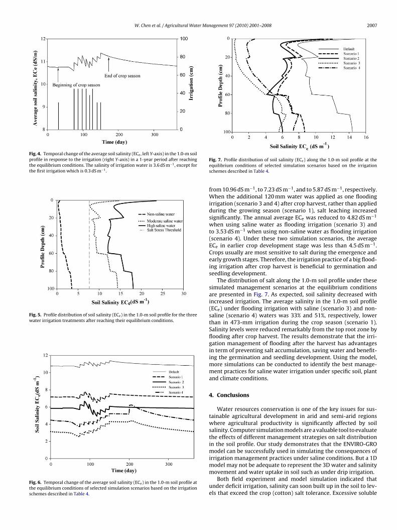

Page 7

W. Chen et al. / Agricultural Water Management 97 (2010) 2001–2008 2007

Fig. 4. Temporal change of the average soil salinity (ECe, left Y-axis) in the 1.0-m soilprofile in response to the irrigation (right Y-axis) in a 1-year period after reachingthe equilibrium conditions. The salinity of irrigation water is 3.6 dS m−1, except forthe first irrigation which is 0.3 dS m−1.

Fig. 5. Profile distribution of soil salinity (ECe) in the 1.0-m soil profile for the threewater irrigation treatments after reaching their equilibrium conditions.

Fig. 6. Temporal change of the average soil salinity (ECe) in the 1.0-m soil profile atthe equilibrium conditions of selected simulation scenarios based on the irrigationschemes described in Table 4.

Fig. 7. Profile distribution of soil salinity (ECe) along the 1.0-m soil profile at theequilibrium conditions of selected simulation scenarios based on the irrigationschemes described in Table 4.

from 10.96 dS m−1, to 7.23 dS m−1, and to 5.87 dS m−1, respectively.When the additional 120 mm water was applied as one floodingirrigation (scenario 3 and 4) after crop harvest, rather than appliedduring the growing season (scenario 1), salt leaching increasedsignificantly. The annual average ECe was reduced to 4.82 dS m−1

when using saline water as flooding irrigation (scenario 3) andto 3.53 dS m−1 when using non-saline water as flooding irrigation(scenario 4). Under these two simulation scenarios, the averageECe in earlier crop development stage was less than 4.5 dS m−1.Crops usually are most sensitive to salt during the emergence andearly growth stages. Therefore, the irrigation practice of a big flood-ing irrigation after crop harvest is beneficial to germination andseedling development.

The distribution of salt along the 1.0-m soil profile under thesesimulated management scenarios at the equilibrium conditionsare presented in Fig. 7. As expected, soil salinity decreased withincreased irrigation. The average salinity in the 1.0-m soil profile(ECe) under flooding irrigation with saline (scenario 3) and non-saline (scenario 4) waters was 33% and 51%, respectively, lowerthan in 473-mm irrigation during the crop season (scenario 1).Salinity levels were reduced remarkably from the top root zone byflooding after crop harvest. The results demonstrate that the irri-gation management of flooding after the harvest has advantagesin term of preventing salt accumulation, saving water and benefit-ing the germination and seedling development. Using the model,more simulations can be conducted to identify the best manage-ment practices for saline water irrigation under specific soil, plantand climate conditions.

4. Conclusions

Water resources conservation is one of the key issues for sus-tainable agricultural development in arid and semi-arid regionswhere agricultural productivity is significantly affected by soilsalinity. Computer simulation models are a valuable tool to evaluatethe effects of different management strategies on salt distributionin the soil profile. Our study demonstrates that the ENVIRO-GROmodel can be successfully used in simulating the consequences ofirrigation management practices under saline conditions. But a 1Dmodel may not be adequate to represent the 3D water and salinity

movement and water uptake in soil such as under drip irrigation.

Both field experiment and model simulation indicated thatunder deficit irrigation, salinity can soon built up in the soil to lev-els that exceed the crop (cotton) salt tolerance. Excessive soluble

Page 8

2 er Man

sesfli

A

RN

R

A

A

B

B

C

D

F

F

F

F

G

H

H

H

203–219.Wang, Y.G., Xiao, D.N., Li, Y., Li, X.Y., 2008. Soil salinity evolution and its relationship

008 W. Chen et al. / Agricultural Wat

alts in irrigated soils can be leached out of the root zone throughither increasing the amount of irrigation during the growing sea-on or flooding the soil after harvest. Model simulation shows thatooding after harvest is more efficient in reducing soil salinity and

ncreasing crop production.

cknowledgements

We would like to thank for the support of National Basicesearch Program of China (#2009CB85100) and the support ofational Natural Science Foundation of China (#30960210).

eferences

llen, R.G., Pereira, L.S., Raes, D., Smith, M., 1998. Crop evapotranspiration guidelinesfor computing crop water requirements. Paper No. 56, FAO, Rome, Italy.

yers, R.S., Westcot, D.W., 1985. Water quality for agriculture. FAO Irrigation andDrainage Paper 29, FAO, Rome, Italy.

ajwa, M.S., Josan, A.S., Hira, G.S., Singh, N.T., 1986. Effect of sustained saline irriga-tion on soil salinity and crop yields. Irrig. Sci. 7, 27–35.

eltran, J.M., 1999. Irrigation with saline water: benefits and environmental impact.Agric. Water Manage. 40, 183–194.

orwin, D.L., Rhoades, D.J., Simunek, J., 2007. Leaching requirement for soil salin-ity control: steady-state versus transient models. Agric. Water Manage. 90,165–180.

udely, L.M., Ben-Gal, A., Shani, U., 2008. Influence of plant, soil, and water on theleaching fraction. Vadose Zone J. 7, 420–425.

eng, G.L., Meiri, A., Letey, J., 2003a. Evaluation of a model for irrigation managementunder saline conditions. I. Effects on Plant Growth. Soil Sci. Soc. Am. J 67, 71–76.

eng, G.L., Meiri, A., Letey, J., 2003b. Evaluation of a model for irrigation managementunder saline conditions. II. Salt distribution and rooting pattern effects. Soil Sci.Soc. Am. J. 67, 77–80.

orkutsa, I., Sommer, R., Shirokova, Y.I., Lamers, J.P.A., Kienzler, K., Tischbein, B.,Martius, C., Vlek, P.L.G., 2009a. Modeling irrigated cotton with shallow ground-water in the Aral Sea Basin of Uzbekistan. II. Soil salinity dynamics. Irrig. Sci. 27,319–330.

orkutsa, I., Sommer, R., Shirokova, Y.I., Lamers, J.P.A., Kienzler, K., Tischbein, B., Mar-tius, C., Vlek, P.L.G., 2009b. Modeling irrigated cotton with shallow groundwaterin the Aral Sea Basin of Uzbekistan. I. Water dynamics. Irrig. Sci. 27, 331–346.

elhar, L.W., Mantoflou, A., Welty, C., Reyfeldt, K.R., 1985. A review of field scalephysical solute transport processes in saturated and unsaturated porous media.Rep EA-4190, Electro Power Res Ins, Palo Alto, California.

anson, J.D., Ahuja, L.R., Shaffer, M.D., Rojas, K.W., DeCoursey, D.G., Farahani, H.,Johnson, K., 1998. RZWQM: simulating the effects of management on water

quality and crop production. Agric. Syst. 57, 161–195.

ollins, S.E., Ridd, P.V., Read, W.W., 2000. Measurement of the diffusion coefficientfor salt in salt flat and mangrove soils. Wetl. Ecol Manage. 8, 257–262.

ou, Z., Li, P., Gong, J., Wang, Y., 2007. Effect of different soil salinity levels andapplication rates of nitrogen on the growth of cotton under drip irrigation. Chin.J. Soil Sci. 38, 681–686 (in Chinese).

agement 97 (2010) 2001–2008

Hutson, J.L., Wagenet, R.J., 1992. LEACHM: Leaching Estimation and ChemistryModel: A Process based Model of Water and Solute Movement Transformations,Plant Uptake and Chemical Reactions in the Unsaturated Zone. Continuum, vol.2. Water Resources Inst, Cornell University, Ithaca, NY, Version 3.

Khan, S., Xevi, E., Meyer, W.S., 2003. Salt, water, and groundwater management mod-els to determine sustainable cropping patterns in shallow saline groundwaterregions of Australia. J. Crop Prod. 7, 325–340.

Leonard, R.A., Knisel, W.G., Still, D.A., 1987. GLEAMS: groundwater loading effectsof agricultural management systems. Trans. ASAE 30, 1403–1418.

Lyman, W.J., Reidy, P.J., Levy, B., 1992. Mobility and Degradation of Organic Con-taminants in Subsurface Environments. Smoley CK Inc., Chelsea, Michigan, p.217.

Maas, E.V., Grattan, S.R., 1999. Crop yield as affected by salinity. AgriculturalDrainage, Agronomy Monograph no. 38, vol. 13–54, ASA, Madison, WI.

Malash, N.M., Flowers, T.J., Ragab, R., 2008. Effect of irrigation methods, manage-ment and salinity of irrigation water on tomato yield, soil moisture and salinitydistribution. Irrig. Sci. 26, 313–323.

Mohammad, M.J., 2004. Squash yield, nutrient content and soil fertility parametersin response to methods of fertilizer application and rates of nitrogen fertigation.Nutr. Cycl. Agroecosyst. 68, 99–108.

Nash, J.E., Sutcliffe, J.V., 1970. River flow forecasting through conceptual models partI. A discussion of principles. J. Hydrol. 10, 282–290.

Oster, J.D., Wichelns, D., 2003. Economic and agronomic strategies to achieve sus-tainable irrigation. Irrig. Sci. 22, 107–120.

Pang, X.P., Letey, J., 1998. Development and evaluation of ENVIRO-GRO, an integratedwater, salinity, and nitrogen model. Soil Sci. Soc. Am. J. 62, 1418–1427.

Plaut, Z., Carmi, A., Grava, A., 1996. Cotton root and shoot responses to subsur-face drip irrigation and partial wetting of the upper soil profile. Irrig. Sci. 16,107–113.

Ragab, R., Malash, N., Abdel Gawad, G., Arslan, A., Ghaibeh, A., 2005. A holistic genericintegrated approach for irrigation, crop and field management. 1. The SALTMEDmodel and its calibration using field data from Egypt and Syria. Agric. WaterManage. 78, 67–88.

Singh, R., Singh, J., 1996. Irrigation planning in cotton through simulation modeling.Irrig. Sci. 17, 31–36.

Simunek, J., Suarez, D.L., Sejna, M., 1996. The UNSATCHEM software package forsimulating one-dimensional variably saturated water flow, heat flow, carbondioxide production and transport, and solute transport with major ion equi-librium and kinetic chemistry, Version 2. Res. Report No. 141. USDA-ARS, U.S.Salinity Lab., Riverside, CA, 186 pp.

van Genuchten, M.T., 1987. A numerical model for water and solute movement inand below the root zone. Res Report No. 121, USDA-ARS US Salinity Laboratory,Riverside, California.

van Genuchten, M.T., 1980. A closed-form equation for predicting the hydraulicconductivity of unsaturated soils. Soil Sci. Soc. Am. J. 44, 892–898.

van Schilfgaarde, J., 1994. Irrigation—a blessing or a curse. Agric. Water Manage. 25,

with dynamics of groundwater in the oasis of inland river basins: case studyfrom the Fubei region of Xinjiang Province, China. Environ. Monit. Assess. 140,291–302.

Willmott, C.J., 1981. On the validation of model. Phys. Geogr. 2, 184–194.