Evaluating Extreme Hierarchical Multi-label Classification

Proceedings of the 60th Annual Meeting of the Association for Computational LinguisticsVolume 1: Long Papers, pages 5809 - 5819

May 22-27, 2022 c©2022 Association for Computational Linguistics

Evaluating Extreme Hierarchical Multi-label Classification

Enrique AmigóUNED

Madrid, [email protected]

Agustín D. DelgadoUNED

Madrid, [email protected]

Abstract

Several natural language processing (NLP)tasks are defined as a classification problem inits most complex form: Multi-label Hierarchi-cal Extreme classification, in which items maybe associated with multiple classes from a setof thousands of possible classes organized ina hierarchy and with a highly unbalanced dis-tribution both in terms of class frequency andthe number of labels per item. We analyze thestate of the art of evaluation metrics based ona set of formal properties and we define an in-formation theoretic based metric inspired bythe Information Contrast Model (ICM). Exper-iments on synthetic data and a case study onreal data show the suitability of the ICM forsuch scenarios.

1 Introduction

Many natural language processing (NLP) problemsinvolve classification, such as sentiment analysis,entity linking, etc. However, the adequacy of eval-uation metrics is still an open problem. Differentmetrics such as Accuracy, F-measure or Macro Av-erage Accuracy (MAAC) may differ substantially,seriously affecting the system optimization process.For example, assigning all elements to the majorityclass may be very effective according to Accuracyand score low according to MAAC.

In addition, in many scenarios such as taggingin social networks (Coope et al., 2018) or topicidentification (Yu et al., 2019), the classifier mustassign several labels to each item (multi-label clas-sification). This greatly complicates the evaluationproblem since, in addition to the class specificity(frequency), other variables appears such as the dis-tribution of labels per item in the gold standard, theexcess or absence of labels in the system output,

etc.The evaluation problem becomes even more

complicated if we consider hierarchical categorystructures, which are very common in NLP. Forexample, toxic messages are divided into differenttypes of toxicity (Fortuna et al., 2019), named enti-ties could be organized in nested categories (Sekineand Nobata, 2004), etc. In these scenarios, the cat-egory proximity in the hierarchical structure is anadditional variable.

Even, the problem can be further complicated.Extreme Classification scenarios address with thou-sands of highly unbalanced categories (Gupta et al.,2019), where a few categories are very frequentand others completely infrequent (Almagro et al.,2020). In addition, some items have no categoryat all and some have many. An example scenariothat we will use as a case study in this article is thelabelling of adverse events in medical documents.

In this paper, we analyse the state of the art onmetrics for multi-label, hierarchical and extremeclassification problems. We characterize existingmetrics by means of a set of formal properties. Theanalysis shows that different metric families satisfydifferent properties, and that satisfying all of themat the same time is not straightforward.

Then, propose an information-theoretic basedmetric inspired by the Information Contrast Modelsimilarity measure (ICM), which can be particular-ized to simpler scenarios (e.g. flat, single labeled)while keeping its formal properties. Later, we de-fine a set of five tests on synthetic data to compareempirically ICM against existing metrics. Finally,we explore a case study with real data which showsthe suitability of ICM for such extreme scenarios.The paper ends with some conclusions and futurework.

5809

2 Background

In this section, we analyze the literature on thetwo main evaluation problems tackled in this paper:multi-labeling and class hierarchies, keeping thefocus on extreme scenarios (numerous and unbal-anced classes).

2.1 Multi-Label Classification

There are three main ways of generalizing effec-tiveness metrics to the multi-label scenario (Zhangand Zhou, 2014). The first one consists in model-ing the problem as a ranking task, i.e. the systemreturns an ordered label list for each item accordingto their suitability. Some specific ranking metricsapplied in multi-label classification displayed in(Wu and Zhou, 2017) are: Ranking Loss, whichis a ordinal correlation measure, one-error whichis based on Precision at 1, or Average Precision.Although these metrics are very common, they donot take into account the specificity of (unbalanced)classes. Jain et al. proposed the propensity versionsof ranking metrics (Precision@k, nDCG) in orderto weight classes according to their frequency inthe data set (Jain et al., 2016).

Reducing the classification to a ranking problemis specially appropriate in extreme classificationscenarios and simplifies the definition of metrics.However, it also has several disadvantages. First, itrequires the output of the classifier to be in rankingformat, and that does not fit many scenarios. Forexample, annotating posts in social networks re-quires predicting the amount of tags to be assignedto the post. For this reason, we focus on classifi-cation outputs, so ranking based metrics are out ofour scope.

Apart from ranking metrics, multi-label effec-tiveness metrics have been categorized into label-and example-based metrics (Tsoumakas et al.,2010; Zhang and Zhou, 2014). Label-based eval-uation measures assess and average the predictiveperformance for each category as a binary classi-fication problem, where the negative category cor-responds with the other categories. The most pop-ular are the label-based Accuracy (LB-ACC) andF-measure (LB-F)1. The label-based metrics havesome drawbacks. First, they do not consider thedistribution of labels per item. Hits are rewardedindependently of how many labels are associated

1In the single label scenario, the label-based F-measureconverges to the traditional F and the label-based accuracy isproportional to the traditional ACC.

to the item. Second, while items are supposed tobe random samples, classes are not, so the ideaof averaging results across classes is not alwaysconsistent. That is, the metric scores can vary sub-stantially depending on how the category space isconfigured. Finally, if there are a large numberof possible categories (extreme classification), thescore contribution of any label has an upper limit of1|C| , being C the set of categories. This limit can beproblematic, specially when labels are unbalancedand numerous.

On the other hand, the example-based metricscompute for each object, the proximity betweenpredicted and true label sets (s(d) = {cs1, .., csn}and g(d) = {cg1, .., c

gn}). Some popular ways to

match category sets in multi-label classificationevaluation are the Jaccard similarity (EB-JACC)which is computed as |s(d)∩g(d)||s(d)∪g(d)| (Godbole and

Sarawagi, 2004), or the precision(|s(d)∩g(d)||s(d)|

), re-

call(|s(d)∩g(d)||g(d)|

)and their F combination (EB-F).

Another example-based metric is the HammingLoss (EB-HAMM) (Zhang et al., 2006) whichmatching function is defined as: |s(d)XOR g(d)|

|Cg |where Cg represents the set of categories anno-tated in the gold standard. Subset Accuracy (EB-SUBACC) (Ghamrawi and McCallum, 2005) is amore strict measure due to it requires exact match-ing between both category sets. Notice that allexample-based multi-label metrics converge to Ac-curacy in the single-label scenario. On the otherhand, there are some situations in which these met-rics are undefined. If both the gold standard and thesystem output label sets are empty, the maximumscore is usually assigned to the item.

The main drawback of these approaches is thatthey do not take into account the specificity ofclasses (i.e. unbalanced classes in extreme clas-sification). The label propensity applied over preci-sion and recall for single items can solve this lack.Each accurate class in the intersection is weightedaccording to the class propensity pc (Jain et al.,2016):

PropP (i) =

∑c∈s(i)∩g(i)

1pc

|s(i)|

PropR(i) =

∑c∈s(i)∩g(i)

1pc

|g(i)|

The propensity factor pc for each class is com-puted as: pc = 1

1+Ce−A log2(Nc+B) where Nc is

5810

the number of data points annotated with label cin the observed ground truth data set of size Nand A, B are application specific parameters andC = (logN −1)(B+1)A. In our experiments, weset the recommended parameter values A = 0.55and B = 1.5.

However, propensity precision and recall valuesare not upper bounded as 1

pctends to infinite when

pc tends to zero. In order to solve this issue, in ourexperiments we replace the normalization factors|s(i)| and |g(i)| with the accumulation of inversepropensities in the system output or the gold stan-dard. We also add the empty class c∅ in both thesystem output and the gold standard in order tocapture the specificity of classes in the mono-labelscenario:

PropP (i) =

∑c∈s′(i)∩g′(i)

1pc∑

c∈s′(i)1pc

PropR(i) =

∑c∈s′(i)∩g′(i)

1pc∑

c∈g′(i)1pc

where s′(i) = s(i)∪ {c∅} and g′(i) = g(i)∪ {c∅}.Propensity F-measure (PROP-F) is computed asthe harmonic mean of these values.

2.2 Hierarchical ClassificationThere are different taxonomies of hierarchical clas-sification metrics (Costa et al., 2007; Kosmopou-los et al., 2013). Kosmopoulos et al. distinguishbetween pair and set-based metrics. Pair-basedmetrics weight hits or misses according to the dis-tance between categories in the hierarchy. This dis-tance depends on the number of intermediate nodes(Wang et al., 1999; Sun and Lim, 2001), with thedisadvantage that the specificity of the categories isnot taken into account. Depth-based distance met-rics include the class depth in the metric (Blockeelet al., 2002). However, the depth of the node is notsufficient to model its specificity since dependingon their frequency, leaf nodes at the first levels maybe more specific than leaf nodes at deeper levels.

It is possible to compare the predicted and truesingle labels by means of standard ontological sim-ilarity measures such as Leackock and Chodorow(path-based) (Leacock and Chodorow, 1998), Wuand Palmer (Wu and Palmer, 1994), Resnik (depth-based) (Resnik, 1999), Jiang and Conrath (Jiangand Conrath, 1997) or Lin (Lin, 1998) similarities.The last two are based on the notion of Informa-tion Content (IC) or category specificity, i.e., the

amount of items belonging to the category or anyof its descendants.

However, extending pair-based hierarchical met-rics to the multi-label scenario is not straightfor-ward. Sun and Lim extended Accuracy, Precisionand Recall measures for ontological distance basedmetrics (Sun and Lim, 2001). This method hastwo drawbacks. First, it requires defining a neutralhierarchical distance, i.e., an acceptable distancethreshold for range normalization purposes. Thesecond drawback is that it inherits the weaknessesof label-based metrics (see previous section). Bloc-keel et al. proposed computing a kernel and thusdefine a Euclidean distance metric between sumsof class values (Blockeel et al., 2002). The draw-back is that they assume a previously defined dis-tance metric between categories and the origin andbetween different categories. Information basedontological similarity measures such as Jiang andConrath or Lin’s similarity do not have an upperbound which is necessary for the calculation ofaccuracy and coverage.

On the other hand, set-based metrics (alsocalled hierarchical-based) consider the ancestoroverlap (Kiritchenko et al., 2004; Costa et al.,2007). More concretely, hierarchical precision andrecall are computed as the intersection of ancestordivided by the amount of ancestors of the systemoutput category and of the gold standard respec-tively2. Their combination is the Hierarchical F-measure (HF). Since these metrics are based on cat-egory set overlap, they can be applied as examplebased multi-label classification by joining ances-tors and computing the F measure. Their drawbackis that the specificity of categories is not strictlycaptured since they assume a correspondence be-tween specificity and hierarchical deepness. How-ever, this correspondence is not necessarily true.Categories in first levels can be infrequent whereasleaf categories can be very common in the data set.

In this paper, we propose an information theo-retic similarity measure called Information Con-trast Model (ICM). ICM is an example-based met-ric as it is computed per item. Just like HF, ICMis a set-based multi-label metric as it computesthe similarity between category sets. Unlike HF,ICM takes into account the statistical specificity ofcategories.

2In our experiments, when computing the ancestor overlapwe consider the common empty label (root class) in order toavoid undefined situations

5811

3 Formal Properties

In order to define the set of desirable properties,we formalize both the gold standard g and the sys-tem output s as sets of item/category assignments(i, c) ∈ I × C, where I and C represent the set ofitems and categories respectively. We will denoteas P (cj) the probability of items to be classifiedas cj in the gold standard (P ((i, cj) ∈ g|i ∈ I)).We also assume that the categories in the hier-archical structure are subsumed. For instance,items in a PERSON_NAMED_ENTITY categoryare implicitly labeled with the parent categoryNAMED_ENTITY. The common ancestor withmaximum depth is denoted as lso(c1, c2) and thedescendant categories are denoted as Desc(c) in-cluding itself.

Note that we do not claim that all properties arenecessary in any scenario. The purpose of thisarticle is to provide at least one metric that is capa-ble of capturing all aspects simultaneously whennecessary.

The first property is related to hits. In order tomake this aspect independent from the ability ofthe metrics to capture hierarchical relationships ormulti-labeling, we define monotonicity over hits inthe simplest case (flat single label scenario):

Property 1 [Strict Monotonicity] A hit increaseseffectiveness. Given a flat single label categorystructure, if (i, c) ∈ g\s, then3 Eff(s∪{(i, c)}) >Eff(s)

The next two properties state that the specificityof both the predicted and the true category affectsthe metric score. That is, an error or a hit in aninfrequent category should have more effect thanin the majority category. For instance, identifyinga rare symptom in a medical report should be re-warded more than identifying a common maladypresent in the vast majority of patients. In addition,both the specificity of the actual category and thespecificity of the category predicted by the systemmust be taken into account. Again, we make thisaspect independent of hierarchical structures andmulti-labeling.

Property 2 [True Category Specificity] Given aflat single label category distribution, if P (c1) <P (c2) and (i, c1), (i, c2) ∈ g \ s, then Eff(s ∪{(i, c1)}) > Eff(s ∪ {(i, c2)}).Property 3 [Wrong Category Specificity] Given aflat single label category distribution, if P (c1) <

3Notice that x ∈ X \ Y ≡ x ∈ X ∧ x /∈ Y

P (c2) and (i, c1), (i, c2) /∈ g ∪ s, then Eff(s ∪{(i, c1)}) < Eff(s ∪ {(i, c2)}).The following property captures the effect of the hi-erarchical category structure. A common elementof any hierarchical proximity measure is that it ismonotonic with respect to the common ancestor.That is, our brother is always closer to us than ourcousin, regardless of which family proximity crite-rion is applied.In this property we do not considermulti-labelling.

Property 4 [Hierarchical Proximity] Underequiprobable categories (P (c1) = P (c2) =P (c3)), the deepness of the common ancestoraffects similarity. Given a single label hierarchicalcategory structure, if s(i) = ∅, g(i) = c1and lso(c1, c2) ∈ Desc(lso(c1, c3)) thenEff(s ∪ {(i, c2)}) > Eff(s ∪ {(i, c3)}).The last two properties are related with the multi-labeling problem. Property 5 rewards the amountof predicted categories per item.

Property 5 [Multi-label Monotonicity] Theamount of predicted categories increases effective-ness. Given a flat multi-label category structure, if(i, c) ∈ g \ s, then Eff(s ∪ {(i, c)}) > Eff(s)

Property 6 rewards hits on multiple items regardinga single item with multiple categories. To under-stand the motivation for this property, we can con-sider an extreme case. Identifying 1000 symptomsin one patient report is of less health benefit thanidentifying one symptom in 1000 patients.

Property 6 [Label vs. Item Quantity] n hits ondifferent items are more beneficial than n labelsassigned to one item. Given a flat multi-labelcategory distribution, if ∀j = 1..n((j, cj) ∈g \ s) and ∀j = 1..n, i > n((i, cj) ∈ g \ s)then Eff(s ∪ {(1, c1), .., (n, cn)}) > Eff(s ∪{(i, c1), .., (i, cn)}).

4 Metric Analysis

In this section, we analyze existing metrics on thebasis of the proposed formal properties (Table 1).Most of metrics satisfy Strict Monotonicity in sin-gle label scenarios. The label-based metric LB-Fcaptures the true and wrong category specificityvia the recall component. The example-based met-ric PROP-F (modified as described in Section 2)captures these properties via the propensity factor.Notice that the original propensity F-measure doesnot capture the wrong category specificity (Prop-erty 3) given that the pc factor is applied only to

5812

Table 1: Metric and Formal Properties

Family Metrics Constraints

Strict True Wrong Hierarchical Multi-label Label vs.Monotonicity Category Category Proximity Monotonicity Item

Specificity Specificity Quantity

LabelBased

Accuracy (LB-ACC) 3 - - - 3 -F measure (LB-F) 3 3 3 - 3 -

ExampleBased

Jaccard (EB-JACC) 3 - - - 3 3Hamming (EB-HAMM) 3 - - - 3 -Subset Acc. (EB-SUBACC) 3 - - - - 3F-measure (EB-F) 3 - - - 3 3Propensity F (PROP-F) 3 3 3 - 3 3

SetBased Hierarchical F (HF) 3 - - 3 3 3

OntologicalSimilarityMeasures(single-labelclassification)

Leacock and Chodorows 3 - - 3 - -Wu and Palmer 3 - - 3 - -Resnik 3 3 - 3 - -Jiang and Conrath 3 3 3 3 - -Lin’s similarity 3 3 3 3 - -

ICM 3 3 3 3 3 -

hits. In addition, both kind of metrics do not cap-ture hierarchical structures. The contribution ofexample regarding label-based metrics is that, aslabel-based metrics are computed item by item, theproperty Label vs. Item Quantity is satisfied (Prop-erty 6). The exception is EB-HAMM which doesnot normalize the results with respect to the amountof labels assigned to the item.

Unlike previous metrics, the set based F-measure(HF) captures the hierarchical structure (Property4). However, it does not capture the category speci-ficity (properties 2 and 3). Some information-basedontological similarity measures, (Lin and Jiang &Conrath) capture both the category specificity andthe hierarchical structure. However, they are not de-fined for multi-label classification (properties 5 and6). In sum, different metric families satisfy differ-ent properties, and that satisfying all of them at thesame time is not straightforward. The properties ofICM are described in the next section.

5 Information Contrast Model

The Information Contrast Model (ICM) is a simi-larity measure that unifies measures based on bothobject feature sets and Information Theory (Amigóet al., 2020). Given two feature sets A and B, ICMis computed as:

ICM(A,B) = α1IC(A)+α2IC(B)−βIC(A∪B)

Where IC(A) represents the information content(−log(P (A)) of the feature set A. In our scenario,

objects are items to be classified and features arecategories. The intuition is that the more the cat-egory sets are unlikely to occur simultaneously(large IC(A∪B)), the less they are similar. Givena fixed joint IC, the more the category sets arespecific (IC(A) and IC(B)), the more they aresimilar. ICM is grounded on similarity axioms sup-ported by the literature in both information accessand cognitive sciences. In addition, it generalizesthe Pointwise Mutual Information and the Tver-sky’s linear contrast model (Amigó et al., 2020).

5.1 Computing Information ContentThe IC of a single category corresponds with theprobability of items to appear in the category or anyof its descendant. It can be estimated as follows:

IC(c) = −log2(P (c)) ' −log2

(∣∣⋃c′∈{c}∪Desc(c) Ic′

∣∣∣∣⋃c′∈C Ic′

∣∣)

where Ic′ represent the set of items assigned to thecategory c′ and Desc(c) represents the set of de-scendant categories. In order to estimate the IC ofcategory set, we state the following considerations.The first one is that, given two categories A and Bthe common ancestor represents their intersectionin terms of feature sets:

{ci} ∩ {cj} = lso(ci, cj) (1)

The second consideration is that we assume Infor-mation Additivity, i.e. the IC of the union of two

5813

sets is the sum of their IC’s minus the IC of itsintersection:

IC({ci}∪{cj}) = IC(ci)+IC(cj)−I({ci}∩{cj}) (2)

Equations 1 and 2 are enough to compute ICM inthe single label scenario. Generalizing for categorysets:

IC({c1, c2, .., cn}) = IC

(⋃i

{ci}

)=

IC(c1) + IC({c2, .., cn})− IC({c1} ∩ {c2, .., cn})

where, according to the transitivity property;

{c1} ∩ {c2, .., cn} =⋃

i=2..n

({c1} ∩ {ci})

and according to Equation 1, it is equivalent to⋃i=2..n{lso(c1, ci)}. Then, we finally obtain a

recursive function to compute the IC of a categoryset:

IC({c1, c2, .., cn}) =

IC(c1) + IC

( ⋃i=2..n

{ci}

)− IC

( ⋃i=2..n

{lso(c1, ci)}

)

In the case of ICM, it is possible the need forestimating the IC of classes that do not appear inthe gold standard. Therefore, we have not evidenceabout its frequency or probability. We apply asmoothing approach by considering the minimumprobability 1

|I| .

5.2 Parameterization and Formal PropertiesOn the basis of five general similarity axioms, in(Amigó et al., 2020) it is stated that the ICM pa-rameters should satisfy α1, α2 < β < α1 + α2.We propose the parameter values α1 = α2 = 2 anβ = 3. This parameterization leads to the follow-ing instantiations for each particular classificationscenario. In the hierarchical mono-label scenario,it becomes into (equations 1 and 2):

ICM(c1, c2) = −IC(c1)− IC(c2) + 3IC(lso(c1, c2))(3)

which is similar to the Jiang and Conrath onto-logical similarity measure. In the flat multi-labelscenario, it becomes into:

ICM(C,C′) =∑

c∈C∩C′

IC(c)−∑

c∈C\C′

∪C′\C

IC(c) (4)

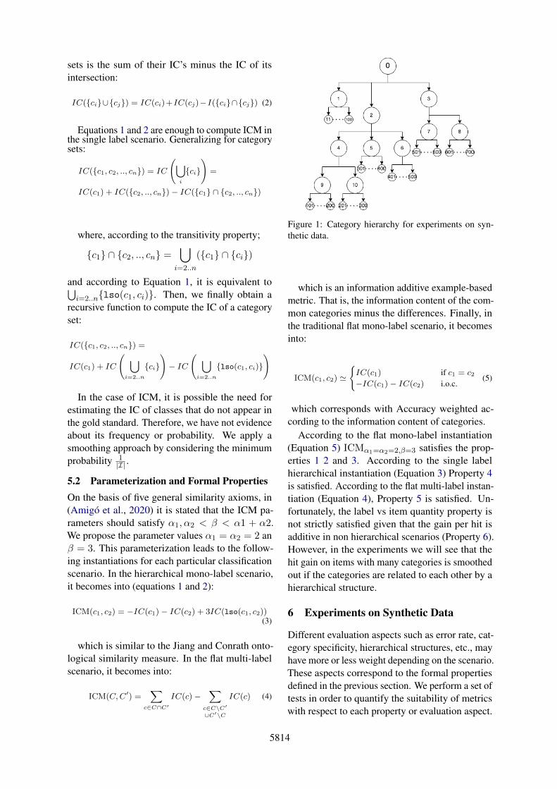
Figure 1: Category hierarchy for experiments on syn-thetic data.

which is an information additive example-basedmetric. That is, the information content of the com-mon categories minus the differences. Finally, inthe traditional flat mono-label scenario, it becomesinto:

ICM(c1, c2) '

{IC(c1) if c1 = c2−IC(c1)− IC(c2) i.o.c.

(5)

which corresponds with Accuracy weighted ac-cording to the information content of categories.

According to the flat mono-label instantiation(Equation 5) ICMα1=α2=2,β=3 satisfies the prop-erties 1 2 and 3. According to the single labelhierarchical instantiation (Equation 3) Property 4is satisfied. According to the flat multi-label instan-tiation (Equation 4), Property 5 is satisfied. Un-fortunately, the label vs item quantity property isnot strictly satisfied given that the gain per hit isadditive in non hierarchical scenarios (Property 6).However, in the experiments we will see that thehit gain on items with many categories is smoothedout if the categories are related to each other by ahierarchical structure.

6 Experiments on Synthetic Data

Different evaluation aspects such as error rate, cat-egory specificity, hierarchical structures, etc., mayhave more or less weight depending on the scenario.These aspects correspond to the formal propertiesdefined in the previous section. We perform a set oftests in order to quantify the suitability of metricswith respect to each property or evaluation aspect.

5814

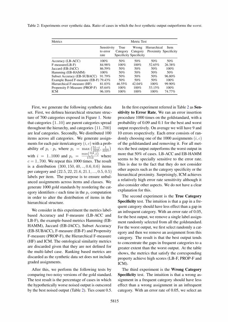
Table 2: Experiments over synthetic data. Ratio of cases in which the best synthetic output outperforms the worst.

Metrics Metric Test

Sensitivity True Wrong Hierarchical Itemto error Category Category Proximity Specificityrate Specificity Specificity

Accuracy (LB-ACC) 100% 50% 50% 50% 50%F-measure(LB-F) 84.98% 100% 100% 52.65% 26.38%Jaccard (EB-JACC) 86.59% 50% 50% 50% 100%Hamming (EB-HAMM) 100% 50% 50% 50% 50%Subset Accuracy (EB-SUBACC) 91.79% 50% 50% 50% 96.80%Example Based F-measure (EB-F) 79.43% 50% 50% 50% 100%Hierarchical F-measure (HF) 81.03% 46.55% 42.04% 100% 99.90%Propensity F-Measure (PROP-F) 85.64% 100% 100% 53.15% 100%ICM 96.10% 100% 100% 100% 74.77%

First, we generate the following synthetic dataset. First, we definea hierarchical structure struc-ture of 700 categories exposed in Figure 1. Notethat categories {1..10} are parent categories spreadthroughout the hierarchy, and categories {11..700}are leaf categories. Secondly, We distributed 100items across all categories. We generate assign-ments for each pair item/category (i, c) with a prob-ability of pi · pc where pi = max

(51−i2225 ,

12225

)with i = 1..1000 and pc =

max( 512c,1)

1713 wherec = 1..700. We repeat this 1000 times. The resultis a distribution (300, 150, 40, .., 0.6, 0.6) itemsper category and (22.5, 22, 21.6, 21.1, ..., 0.5, 0.5)labels per item. The purpose is to ensure unbal-anced assignments across items and classes. Wegenerate 1000 gold standards by reordering the cat-egory identifiers c each time in the pc computationin order to alter the distribution of items in thehierarchical structure.

We consider in this experiment the metrics label-based Accuracy and F-measure (LB-ACC andLB-F), the example-based metrics Hamming (EB-HAMM), Jaccard (EB-JACC), Subset Accuracy(EB-SUBACC), F-measure (EB-F) and PropensityF-measure (PROP-F), the Hierarchical F-measure(HF) and ICM. The ontological similarity metricsare discarded given that they are not defined forthe multi-label case. Ranking based metrics arediscarded as the synthetic data set does not includegraded assignments.

After this, we perform the following tests bycomparing two noisy versions of the gold standard.The test result is the percentage of cases in whichthe hypothetically worse noised output is outscoredby the best noised output (Table 2). Ties count 0.5.

In the first experiment referred in Table 2 as Sen-sitivity to Error Rate, We ran an error insertionprocedure 1000 times on the goldstandard, with aprobability of 0.09 and 0.1 for the best and worstoutput respectively. On average we will have 9 and10 errors respectively. Each error consists of ran-domly choosing one of the 1000 assignments (i, c)of the goldstandard and removing it. For all met-rics the best output outperforms the worst output inmore that 50% of cases. LB-ACC and EB-HAMMseems to be specially sensitive to the error rate.This is due to the fact that they do not considerother aspects such as the category specificity or thehierarchical proximity. Surprisingly, ICM achievesa relatively high error rate sensitivity although italso consider other aspects. We do not have a clearexplanation for this.

The second experiment is the True CategorySpecificity test. The intuition is that a gap in a fre-quent category should have less effect than a gap inan infrequent category. With an error rate of 0.05,for the best output, we remove a single label assign-ment randomly selected from all the goldstandard.For the worst output, we first select randomly a cat-egory and then we remove an assignment from thiscategory. The result is that the best output tendsto concentrate the gaps in frequent categories to agreater extent than the worst output. At the tableshows, the metrics that satisfy the correspondingproperty achieve high scores (LB-F, PROP-F andICM).

The third experiment is the Wrong CategorySpecificity test. The intuition is that a wrong as-signment in a frequent category should have lesseffect than a wrong assignment in an infrequentcategory. With an error rate of 0.05, we select an

5815

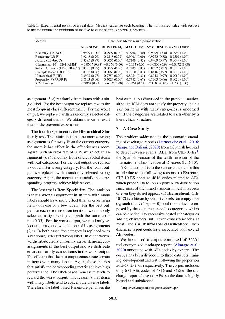
Table 3: Experimental results over real data. Metrics values for each baseline. The normalised value with respectto the maximum and minimum of the five baseline scores is shown in brackets.

Metrics Baselines: Metric result (normalization)

ALL NONE MOST FREQ. MATCH 75% SVM DESCR. SVM CODES

Accuracy (LB-ACC) 0.9999 (1.00) 0.9997 (0.00) 0.9998 (0.50) 0.9999 (1.00) 0.9999 (1.00)F-measure(LB-F) 0.9248 (0.79) 0.9248 (0.79) 0.9005 (0.00) 0.9273 (0.88) 0.9309 (1.00)Jaccard (EB-JACC) 0.8395 (0.97) 0.0055 (0.00) 0.7209 (0.83) 0.8409 (0.97) 0.8644 (1.00)-Hamming×103 (EB-HAMM) −0.0507 (0.98) −0.254 (0.00) −0.117 (0.66) −0.0506 (0.98)−0.0472 (1.00)Subset Accuracy (EB-SUBACC) 0.8395 (0.97) 0.0027 (0.00) 0.7205 (0.83) 0.8392 (0.97) 0.8573 (1.00)Example Based F (EB-F) 0.8395 (0.96) 0.0066 (0.00) 0.7210 (0.83) 0.8416 (0.97) 0.8670 (1.00)Hierarchical F (HF) 0.8902 (0.97) 0.2750 (0.00) 0.8054 (0.83) 0.8913 (0.97) 0.9080 (1.00)Propensity F (PROP-F) 0.8893 (0.96) 0.5024 (0.00) 0.7742 (0.67) 0.8903 (0.96) 0.9030 (1.00)ICM Average -2.2062 (0.92) -8.6158 (0.00) -5.5761 (0.43) -2.1107 (0.94) -1,700 (1.00)

assignment (i, c) randomly from items with a sin-gle label. For the best output we replace c with themost frequent class different than c. For the worstoutput, we replace c with a randomly selected cat-egory different than c. We obtain the same resultthan in the previous experiment.

The fourth experiment is the Hierarchical Sim-ilarity test. The intuition is that the more a wrongassignment is far away from the correct category,the more it has effect in the effectiveness score.Again, with an error rate of 0.05, we select an as-signment (i, c) randomly from single labeled itemswith leaf categories. For the best output we replacec with a sister wrong category. For the worst out-put, we replace c with a randomly selected wrongcategory. Again, the metrics that satisfy the corre-sponding property achieve high scores.

The last test is Item Specificity. The intuitionis that a wrong assignment in an item with manylabels should have more effect than an error in anitem with one or a few labels. For the best out-put, for each error insertion iteration, we randomlyselect an assignment (i, c) (with the same errorrate 0.05). For the worst output, we randomly se-lect an item i, and we take one of its assignments(i, c). In both cases, the category is replaced witha randomly selected wrong label. In other words,we distribute errors uniformly across item/categoryassignments in the best output and we distributeerrors uniformly across items in the worst output.The effect is that the best output concentrates errorsin items with many labels. Again, those metricsthat satisfy the corresponding metric achieve highperformance. The label-based F-measure tends toreward the worst output. The reason is that itemswith many labels tend to concentrate diverse labels.Therefore, the label-based F measure penalizes the

best output. As discussed in the previous section,although ICM does not satisfy the property, the hitgain on items with many categories is smoothedout if the categories are related to each other by ahierarchical structure.

7 A Case Study

The problem addressed is the automatic encod-ing of discharge reports (Dermouche et al., 2016;Bampa and Dalianis, 2020) from a Spanish hospitalto detect adverse events (AEs) from CIE-10-ES4,the Spanish version of the tenth revision of theInternational Classification of Diseases (ICD-10).

AEs detection fits to the scenario tackled in thisarticle due to the following reasons: (i) Extreme:CIE-10-ES contains 4816 codes related to AEs,which probability follows a power-law distributionsince most of them rarely appear in health recordsor even they do not appear; (ii) Hierarchical: CIE-10-ES is a hierarchy with six levels: an empty root(c∅ such that IC(c∅) = 0), and then a level com-posed by three-character-codes categories whichcan be divided into successive nested subcategoriesadding characters until seven-character-codes atmost; and (iii) Multi-label classification: Eachdischarge report could have associated with severalAEs codes.

We have used a corpus composed of 36264real anonymized discharge reports (Almagro et al.,2020) annotated with AEs codes by experts. Thecorpus has been divided into three data sets, train-ing, development and test, following the proportion50%-30%-20% respectively. The corpus includesonly 671 AEs codes of 4816 and 84% of the dis-charge reports have no AEs, so the data is highlybiased and unbalanced.

4https://eciemaps.mscbs.gob.es/ecieMaps/

5816

We have applied five simple baselines in orderto analyze the behaviour of the metrics: (i) ALLNONE does not assign any code to each item;(ii) MOST FREQ. assigns the most frequent AEcode in the training data set (T45.1X5A) to eachitem, which just appears in 68 items of 7253; (iii)MATCH 75% divides each item into sentencesand assigns a code if a sentence contains 75% of thewords of the code description avoiding stop-words;(iv) SVM DESCR. creates a binary classifier foreach AE code in the training set using the pres-ence of words of the AEs codes descriptions in theitems as features, excepting stop-words; (v) SVMCODES: similar to the previous one but using asfeatures the annotated non-AEs codes in order tocheck if AEs codes are related to non-AEs codes.Note that MATCH 75% is able to assign any AE,but the SVM baselines are only able to assign AEsappearing in the training data set.

Table 3 shows the metrics results obtained byeach baseline. Unfortunately, with only five sys-tems it is difficult to find differences in terms ofsystem ranking. Therefore, we have normalised thevalues for each metric between the maximum andthe minimum obtained across the 5 systems in orderto study the relative differences of scores (values inbrackets). LB-ACC, LB-F and EB-HAMM rewardthe absence of most of the labels in the corpus, sothey are not suitable in this scenario. The rest ofthe metrics sort systems in the same way. The par-ticularity of ICM is that, as shows the normalizedresults, the baseline MATCH 75% is penalized withrespect to ALL NONE to a greater extent than inother metrics, since MATCH 75% assigns manycodes incorrectly, whereas ALL NONE does notprovide any information. Another slight particu-larity of ICM is that the system SVM CODES isrewarded against the rest of baselines to a greaterextent. Notice that SVM CODES achieves 269 hitswhile SVM DESCR achieves 77 hits.

8 Conclusions and Future Work

The definition of evaluation metrics is an openproblem for extreme hierarchical multi-label clas-sification scenarios due to the role of several vari-ables, for instance, a huge number of labels, un-balanced and biased label and item distributions,proximity between classes into the hierarchy, etc.Our formal analysis shows that metrics from differ-ent families (label, example, set-based, ontologicalsimilarity measures etc.) satisfy different proper-

ties and capture different evaluation aspects. Theinformation-theoretic metric ICM proposed in thispaper, combines strengths from different families.Just like example-based multi-label metrics, it com-putes scores by items. Just like set-based metrics, itcompares hierarchical category sets. Just like someontological similarity measures (Lin or Jiang andConrath), it considers the specificity of categoriesin terms of Information Content. Our experimentsusing synthetic and real data show the suitabilityof ICM with respect to existing metrics.

ICM does not strictly hold the label vs. itemquantity property. We propose to adapt ICM in or-der to guarantee all the formal properties as futurework.

Acknowledgments

Research cooperation between UNED and theSpanish Ministry of Economy and Competitive-ness, ref. C039/21-OT and in the framework ofDOTT-HEALTH project (MCI/AEI/FEDER, UE)under Grant PID2019-106942RB-C32.

ReferencesMario Almagro, Raquel Martínez, Víctor Fresno, and

Soto Montalvo. 2020. ICD-10 coding of spanishelectronic discharge summaries: An extreme classi-fication problem. IEEE Access, 8:100073–100083.

Enrique Amigó, Fernando Giner, Julio Gonzalo, andFelisa Verdejo. 2020. On the foundations of simi-larity in information access. Inf. Retr. J., 23(3):216–254.

Maria Bampa and Hercules Dalianis. 2020. Detectingadverse drug events from Swedish electronic healthrecords using text mining. In Proceedings of theLREC 2020 Workshop on Multilingual BiomedicalText Processing (MultilingualBIO 2020), pages 1–8, Marseille, France. European Language ResourcesAssociation.

Hendrik Blockeel, Maurice Bruynooghe, Saso Dze-roski, Jan Ramon, and Jan Struyf. 2002. Hierar-chical multi-classification. Workshop Notes of theKDD’02 Workshop on Multi-Relational Data Min-ing, pages 21–35.

Sam Coope, Yoram Bachrach, Andrej Zukov Gregoric,José Rodríguez, Bogdan Maksak, Conan McMurtie,and Mahyar Bordbar. 2018. A neural architecturefor multi-label text classification. In Intelligent Sys-tems and Applications - Proceedings of the 2018 In-telligent Systems Conference, IntelliSys 2018, Lon-don, UK, September 6-7, 2018, Volume 1, volume868 of Advances in Intelligent Systems and Comput-ing, pages 676–691. Springer.

5817

Eduardo P. Costa, Ana C. Lorena, Andre C.P.L.F. Car-valho, and Alex A. Freitas. 2007. A review of per-formance evaluation measures for hierarchical clas-sifiers. AAAI Workshop - Technical Report.

Mohamed Dermouche, Julien Velcin, Rémi Flicoteaux,Sylvie Chevret, and Namik Taright. 2016. Super-vised topic models for diagnosis code assignment todischarge summaries. In Computational Linguisticsand Intelligent Text Processing - 17th InternationalConference, CICLing 2016, Konya, Turkey, April 3-9, 2016, Revised Selected Papers, Part II, volume9624 of Lecture Notes in Computer Science, pages485–497. Springer.

Paula Fortuna, João Rocha da Silva, Juan Soler-Company, Leo Wanner, and Sérgio Nunes. 2019.A hierarchically-labeled Portuguese hate speechdataset. In Proceedings of the Third Workshop onAbusive Language Online, pages 94–104, Florence,Italy. Association for Computational Linguistics.

Nadia Ghamrawi and Andrew McCallum. 2005. Col-lective multi-label classification. In Proceedingsof the 14th ACM International Conference on In-formation and Knowledge Management, CIKM ’05,page 195–200, New York, NY, USA. Association forComputing Machinery.

Shantanu Godbole and Sunita Sarawagi. 2004. Dis-criminative methods for multi-labeled classification.In Advances in Knowledge Discovery and DataMining, pages 22–30, Berlin, Heidelberg. SpringerBerlin Heidelberg.

Vivek Gupta, Rahul Wadbude, Nagarajan Natarajan,Harish Karnick, Prateek Jain, and Piyush Rai. 2019.Distributional semantics meets multi-label learning.In The Thirty-Third AAAI Conference on ArtificialIntelligence, AAAI 2019, Honolulu, Hawaii, USA,pages 3747–3754. AAAI Press.

Himanshu Jain, Yashoteja Prabhu, and Manik Varma.2016. Extreme multi-label loss functions for rec-ommendation, tagging, ranking & other missinglabel applications. In Proceedings of the 22ndACM SIGKDD International Conference on Knowl-edge Discovery and Data Mining, KDD ’16, page935–944, New York, NY, USA. Association forComputing Machinery.

Jay J. Jiang and David W. Conrath. 1997. Semanticsimilarity based on corpus statistics and lexical tax-onomy. In Proc. of the Int’l. Conf. on Research inComputational Linguistics, pages 19–33.

Svetlana Kiritchenko, Stan Matwin, and Fazel Famili.2004. Hierarchical text categorization as a tool of as-sociating genes with gene ontology codes. Proceed-ings of the 2nd European Workshop on Data Miningand Text Mining in Bioinformatics.

Aris Kosmopoulos, Ioannis Partalas, Eric Gaussier,Georgios Paliouras, and Ion Androutsopoulos. 2013.Evaluation measures for hierarchical classification:

a unified view and novel approaches. Data Miningand Knowledge Discovery, 29.

Claudia Leacock and Martin Chodorow. 1998. Com-bining local context and wordnet similarity for wordsense identification. WordNet: An electronic lexicaldatabase, 49(2):265–283.

Dekang Lin. 1998. An information-theoretic definitionof similarity. In Proceedings of the Fifteenth Inter-national Conference on Machine Learning (ICML1998), Madison, Wisconsin, USA, July 24-27, 1998,pages 296–304. Morgan Kaufmann.

Philip Resnik. 1999. Semantic similarity in a taxon-omy: An information-based measure and its applica-tion to problems of ambiguity in natural language. J.Artif. Intell. Res., 11:95–130.

Satoshi Sekine and Chikashi Nobata. 2004. Definition,dictionaries and tagger for extended named entity hi-erarchy. In Proceedings of the Fourth InternationalConference on Language Resources and Evaluation(LREC’04), Lisbon, Portugal. European LanguageResources Association (ELRA).

Aixin Sun and Ee-Peng Lim. 2001. Hierarchical textclassification and evaluation. In Proceedings of the2001 IEEE International Conference on Data Min-ing, 29 November - 2 December 2001, San Jose, Cal-ifornia, USA, pages 521–528. IEEE Computer Soci-ety.

Grigorios Tsoumakas, Ioannis Katakis, and Ioannis P.Vlahavas. 2010. Mining multi-label data. In DataMining and Knowledge Discovery Handbook, 2nded, pages 667–685. Springer.

Ke Wang, Senqiang Zhou, and Shiang Chen Liew.1999. Building hierarchical classifiers using classproximity. In VLDB’99, Proceedings of 25th In-ternational Conference on Very Large Data Bases,September 7-10, 1999, Edinburgh, Scotland, UK,pages 363–374. Morgan Kaufmann.

Xi-Zhu Wu and Zhi-Hua Zhou. 2017. A unifiedview of multi-label performance measures. In Pro-ceedings of the 34th International Conference onMachine Learning - Volume 70, ICML’17, page3780–3788. JMLR.org.

Zhibiao Wu and Martha S. Palmer. 1994. Verb seman-tics and lexical selection. In 32nd Annual Meet-ing of the Association for Computational Linguistics,27-30 June 1994, New Mexico State University, LasCruces, New Mexico, USA, Proceedings, pages 133–138. Morgan Kaufmann Publishers / ACL.

Dongjin Yu, Dengwei Xu, Dongjing Wang, and Zhiy-ong Ni. 2019. Hierarchical topic modeling of twitterdata for online analytical processing. IEEE Access,7:12373–12385.

Min-Ling Zhang and Zhi-Hua Zhou. 2014. A re-view on multi-label learning algorithms. IEEETransactions on Knowledge and Data Engineering,26(8):1819–1837.

5818

Yi Zhang, Samuel Burer, and W. Nick Street.2006. Ensemble pruning via semi-definite pro-gramming. Journal of Machine Learning Research,7:1315–1338.

5819