Evaluating choices in multi-process landscape evolution models

Geomorphology 125 (2011) 271–281

Contents lists available at ScienceDirect

Geomorphology

j ourna l homepage: www.e lsev ie r.com/ locate /geomorph

Evaluating choices in multi-process landscape evolution models

A.J.A.M. Temme a,⁎, L. Claessens a,b, A. Veldkamp c, J.M. Schoorl a

a Land Dynamics group, Wageningen University, PO Box 47, 6700 AA Wageningen, The Netherlandsb International Potato Center (CIP), PO Box 25171, Nairobi 00603, Kenyac Faculty of Geo-Information Science and Earth Observation (ITC), University of Twente, PO Box 6, 7500 AA Enschede, The Netherlands

⁎ Corresponding author. Tel.: +31 3174 84445; fax: +E-mail address: [email protected] (A.J.A.M. Tem

0169-555X/$ – see front matter © 2010 Elsevier B.V. Adoi:10.1016/j.geomorph.2010.10.007

a b s t r a c t

Article history:Received 14 November 2009Received in revised form 27 September 2010Accepted 3 October 2010Available online 8 October 2010

Keywords:Landscape evolution modelGeomorphic processLAPSUSEquifinalityLandscape processModel performance

The interest in landscape evolution models (LEMs) that simulate multiple landscape processes is growing.However, modelling multiple processes constitutes a new starting point for which some aspects of the set upof LEMs must be re-evaluated. The objective of this paper is to demonstrate the practical significance of, andpossibilities for such re-evaluation. We first discuss which simplifications must be made to set up LEMs. Then,simplifications of particular interest to the modelling of multiple processes are identified. Finally, case studiesfrom New Zealand, Belgium and Croatia explore the performance of different model versions under severalcommon choices for model and data simplifications. In these case studies we illustrate methods to make thechoices, typically by i) comparing the results of different model versions, ii) assessing model validity or iii)indicating the sensitivity of models for different simplifications. The results indicate that LEM performance isstrongly dependent onmulti-process related choices, and that performance indicators can be used for ex-posttesting of the influence of these choices. In particular, we demonstrate the significance of simplificationsregarding the number of processes, presence of sinks and temporal resolution.

31 3174 19000.me).

ll rights reserved.

© 2010 Elsevier B.V. All rights reserved.

1. Introduction

Many processes result in landscape change. How these landscapeprocesses act and interact is a topic of continuing interest forgeomorphology. Landscape evolution models (LEMs) can play animportant role in pursuing this interest, given their potential role inhypothesis generation about landscape evolution and interactionsbetween processes in space and time (e.g. Coulthard, 2001). Both thedevelopment of LEMs themselves, as the interpretation of simulationresults, may lead to improved understanding of landscape evolution.

Within current literature, no clear definition of LEMs is provided(Pazzaglia, 2003). Arguably, such a definition should focus onobjectives, rather than methods. A recent review on models focussingon fluvial and hillslope processes is given by Tucker and Hancock(2010). In addition, Brasington and Richards (2007) suggest that LEMscharacteristically focus on landscape dynamics at spatial extents of100–102 km2 and temporal extents of 101–103 years. This focus is anexpression of both (diminishing) computational and (more perma-nent) data constraints as much as that of the objectives. Therefore,adaptation of these extents is warranted. Here, we choose to discussLEMs that focus on landscape dynamics at spatial extents larger than100 km2 and at temporal extents between 101 and 104 years.Consequently, we operate at the lower end of geological timescales,

where we safely may reduce the influence of climate, base levelchange, tectonics, and weathering.

LEM studies that model a single landscape process outnumberthose that model multiple processes. Recent work has been done onfor example water erosion and deposition (Takken et al., 1999;Schoorl and Veldkamp, 2001; Collins et al., 2004), tillage erosion(Heuvelink et al., 2006), landsliding (Claessens et al., 2005, 2007),weathering (Heimsath et al., 1997; Minasny and McBratney, 2001),soil creep (Minasny and McBratney, 1999, 2001, 2006), fluvial action(Coulthard et al., 1998, 2000, 2002) and dune formation (Baas, 2007;Baas and Nield, 2007). To a large degree these studies aimed atdevelopment and validation of process descriptions. For otherlandscape processes, empirical identification of controls is ongoingand landscape-scale process descriptions are still premature. Exam-ples are wind erosion (Okin et al., 2006), gelifluction (Harris et al.,2003), solifluction (Matsuoka et al., 2005) and frost weathering(Williams and Robinson, 2001). At the same time, the interest instudying multiple processes and their interactions in the landscape isgrowing, particularly in combination with the increased focus onreduced complexity modelling in fluvial geomorphology (Brasingtonand Richards, 2007), which stresses the simplification of processknowledge required for landscape-scale LEMs.

Simplification or reducing complexity is part of every modellingexercise, with single-process LEMs included. Recent LEM studies haveused reduced complexity as a way to focus on multiple processes andtheir interactions. The combination of water and tillage erosionreceived early attention in agricultural landscapes in Belgium (Goverset al., 1996; Peeters et al., 2006) and later in Spain (Schoorl et al.,

272 A.J.A.M. Temme et al. / Geomorphology 125 (2011) 271–281

2004). Follain et al. (2006) simulated the combined effect of soil creepand water erosion in an agricultural landscape in France; Coulthardand Van de Wiel (2006) and Van de Wiel et al. (2007) combinedseveral processes in the fluvial domain in Wales; and Temme andVeldkamp (2009) combined water erosion, biological and frostweathering, creep and solifluction in a study of a valley in SouthAfrica. Coulthard and Baas (2008) combined aeolian dune activity andfluvial activity using an example from Mongolia.

Attention for the interactions between geomorphic landscapeprocesses and land use and cover change processes is also increasing(Veldkamp et al., 2001). Claessens et al. (2009) modelled interactionsand feedback mechanisms between landscape processes watererosion and deposition and tillage on the one hand and land usechange on the other hand.

Frameworks for LEMs increasingly include multiple processes in amodular setup. Frameworks that combine processes include CHILD(Tucker et al., 2001), CAESAR (Coulthard et al., 1998), LAPSUS(Schoorl et al., 2000, 2002), SIBERIA (Willgoose et al., 1990), CASCADE(Braun and Sambridge, 1997) and WATEM (Van Oost et al., 2000).

The modelling of multiple processes in a dynamic landscapeconstitutes a new starting point for which common model and datasimplifications have to be re-evaluated. The objective of this paper isto perform such re-evaluation. First, we discuss the simplificationsthat are necessary to set up case-specific optimal LEMs and identifysimplifications of particular importance for multi-process LEMs. Then,we use case studies to illustrate how some of these simplificationsaffect multi-process LEM performance. Simplifications regarding thenumber of processes, the presence of sinks and temporal resolutionare considered. The case studies are intended to help chooseappropriate simplifications in other studies.

The focus of this paper is on the effects of model and datasimplifications in multi-process model setup, not on the descriptionsof individual processes or their validity. Therefore, the discussion ofthe process descriptions is kept brief and no topical conclusions aredrawn in the presented case studies. Furthermore, the focus is onLEMs as defined previously, particularly those that use digitalelevation models (DEMs) as their digital landscape, although theresults may be applicable wider afield.

2. Simplifications in landscape evolution modelling

All geomorphologists distinguish different landscape processes.Changes in landscapes are thought to be the result of discretegeomorphic processes and many are described in mono-geneticterms. Obviously, these single-process changes may interact andaccumulate as they do in multi-process LEMs.

It might be argued that what can be seen as discrete geomorphicprocesses, are actually sets of landscape activities that are arbitrarilydefined in a multi-dimensional space of material properties andaffecting forces. Problematically, in such space, geomorphology's self-defined “processes” are scale-dependent, may overlap with others orleave space in between processes. Consequently, landscape activitymight be described twice or not at all. This way of thinking may haveprofound implications for multi-process modelling and is one of ourcontinuing research interests.

Nevertheless, we accept for the moment that processes aredistinguished, and we tentatively define an ideal LEM as calculatingcorrect quantities of change in the correct location and moment for alllandscape processes. In other words, there are four requirements: allprocesses, correct location, correct moment and correct quantity.Meeting these requirements and starting with correct boundaryconditions entails that every process acts on a correctly modelledlandscape in every timestep. If it is also assumed that processes onlyinfluence other processes through changes in the landscape, thencorrect landscape evolution modelling is achieved. To our knowledge,this last assumption is made in all considered models, yet it may be

relaxed when a need is perceived for processes to interact through forinstance climate or vegetation changes. In future landscape evolutionstudies at continental or global scale, landscape processes may forinstance influence climate (perhaps throughnet carbon sequestration;Liu et al., 2003), which in turn influences other landscape processes.

In all modelling studies, simplifications of model assumptions anddata are necessary. These simplifications encompass all steps taken toget from our real-world perception of a changing landscape to anLEM (cf. Beven, 2009). They include the reduction in complexity ofprocess descriptions meant by Brasington and Richards (2007).Here, simplifications affecting the ideal LEM defined above arediscussed in more detail: 1) processes, 2) space or location, 3) timeand 4) quantities. Simplifications of particular interest for multi-process LEMs are identified.

2.1. Processes

The first requirement is that all landscape processes are included. Afirst simplification in LEMs is to only include case-relevant processes—known in hydrology as the dominant process approach (Sivakumar,2008). In single-process LEM studies, this simplification is madeimplicitly, but in multi-process LEMs a more explicit consideration isrequired.

A first aspect of process-relevance is arguably the mass or volumetransported or transformed. Processes transporting more material aremore relevant to landscape evolution. However, relevance of a processfor a study is not necessarily defined in terms of the volume ittransports itself. For instance, landslides can dam valleys and havelarge-scale and long-term consequences for up- and downstreamerosion and deposition (e.g. Korup, 2002). That can be a reason toinclude them in a multi-process LEM study even if much less materialis involved in landsliding than in other processes.

Ideally, information about relevance follows from field observa-tions. Relevance of a process can only be defined in terms of a positiveeffect on model performance if sufficient independent observationsare available. This is problematic when fieldwork and dating effortshave mostly been focussed on one landscape process. In that case,model simulations can merely explore which processes are relevant.We demonstrate such an exploration in case study A.

2.2. Space

Implementations of processes must model process activity in thecorrect location. The typical discretization (simplification) of spaceinto finite elements, and one that this paper is limited to, is tosubdivide the spatial extent into rows and columns of square surfaceswith uniform altitude (cells) in DEMs. Alternatively, space can bedivided into Delaunay triangles resulting in Triangulated IrregularNetworks (TINs). These TINs have the advantage that the triangularsurfaces do not need to have uniform altitude and that data densitycan vary within the spatial extent. The primary disadvantage of TINs isthe difficulty in developing process descriptions. LEM frameworkssuch as CASCADE (Braun and Sambridge, 1997) and CHILD (e.g.Tucker et al., 2001) use these TINs.

Model results are sensitive to the discretization of space,essentially because process spatial resolutions differ from modelspatial resolutions (Grayson et al., 1992). This leads to resolutiondependency of parameters in process descriptions and, consequently,of finalmodel results (e.g. Thompson et al., 2001). Spatial resolution ofprocesses in LEMs is a better-studied simplification than othersdiscussed in this section (e.g. Coulthard et al., 1998; Schoorl et al.,2000; Claessens et al., 2005; Hancock, 2006), and its effect onmultipleprocesses is expected to be similar. It will therefore not be studied in acase study here.

Given the discretization into grid cells, the second requirementtranslates into a requirement to model process activity in the correct

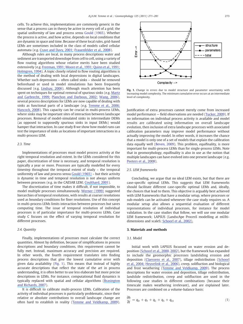
Fig. 1. Change in errors due to model structure and parameter uncertainty withincreasing model complexity. Theminimum cumulative error occurs at an intermediatelevel of complexity.

273A.J.A.M. Temme et al. / Geomorphology 125 (2011) 271–281

cells. To achieve this, implementations are commonly generic in thesense that a process can in theory be active in every cell of a grid; thespatial uniformity of law and process sensu Gould (1965). Whetherthe process is active, and how active, depends on local conditions thatare dynamic in space and time. Because of these local rules, grid-basedLEMs are sometimes included in the class of models called cellularautomata (e.g. Crave and Davy, 2001; Frauenfelder et al., 2008).

Although rules are local, in many process descriptions water andsediment are transporteddownslope from cell to cell, using a variety offlow routing algorithms whose relative merits have been studiedextensively (e.g. Freeman, 1991;Moore et al., 1991; Quinn et al., 1991;Holmgren, 1994). A topic closely related to flow routing algorithms isthe method of dealing with local depressions in digital landscapes.Whether such depressions – often called sinks – should be removedbeforehand or used in model simulations has been frequentlydiscussed (e.g. Lindsay, 2006). Although much attention has beenspent on techniques for optimal removal of spurious sinks (e.g. Martzand Garbrecht, 1999; Planchon and Darboux, 2002; Wang, 2006),several process descriptions for LEMs are now capable of dealing withsinks as functional parts of a landscape (e.g. Temme et al., 2006;Hancock, 2008). This capacity can be crucial in multi-process LEMs,where sinks may be important sites of interaction between landscapeprocesses. Removal of model-simulated sinks in intermediate DEMs(as opposed to supposedly spurious sinks in input DEMs) wouldhamper that interaction. In case study B we show howmodel runs cantest the importance of sinks as locations of important interactions in amulti-process LEM.

2.3. Time

Implementations of processes must model process activity at theright temporal resolution and extent. In the LEMs considered for thispaper, discretization of time is necessary, and temporal resolution istypically a year or more. Processes are typically modelled for everytimestep throughout the temporal extent of study – the temporaluniformity of law and process sensu Gould (1965) – but their activityis dynamic in time and temporal resolution is not always uniformbetween processes (e.g. in the CAESAR LEM; Coulthard, 2001).

The discretization of time makes it difficult, if not impossible, tomodel multiple processes simultaneously. Werner (1999) suggestedhierarchies of temporal resolutions, with results at coarser resolutionsused as boundary conditions for finer resolutions. Use of this conceptin multi-process LEMs limits interaction between processes but savescomputing time. The issue of temporal resolution of individualprocesses is of particular importance for multi-process LEMs. Casestudy C focuses on the effect of varying temporal resolution fordifferent processes.

2.4. Quantity

Finally, implementations of processes must calculate the correctquantities. Almost by definition, because of simplifications in processdescriptions and boundary conditions, this requirement cannot befully met. Instead, maximum accuracy and precision are required.In other words, the fourth requirement translates into findingprocess descriptions that give the lowest cumulative error withgiven data availability (Fig. 1). This means that instead of highlyaccurate descriptions that reflect the state of the art in processunderstanding, it is often better to use less elaborate but more precisedescriptions in LEMs. For instance, computational fluid dynamics istypically replaced with spatial and cellular algorithms (Brasingtonand Richards, 2007).

It is difficult to calibrate multi-process LEMs. Calibration of theactivity of individual processes is particularly problematic, since theirrelative or absolute contributions to overall landscape change areoften hard to establish in reality (Temme and Veldkamp, 2009).

Justification of extra processes cannot merely come from increasedmodel performance— field observations are needed (Tucker, 2009). Ifno information on individual process activity is available and modelresults are calibrated using information on overall landscapeevolution, then inclusion of extra landscape processes with associatedcalibration parameters may improve model performance withoutactually improving the model. In other words, it increases the chancethat a model is only one of a set of models that explain the calibrationdata equally well (Beven, 2009). This problem, equifinality, is moreimportant for multi-process LEMs than for single-process LEMs. Notethat in geomorphology, equifinality is also in use as the notion thatmultiple landscapes can have evolved into one present landscape (e.g.Peeters et al., 2008).

2.5. LEM frameworks

Concluding, we argue that no ideal LEM exists, but that there arecase-specific optimal LEMs. This suggests that LEM frameworksshould facilitate different case-specific optimal LEMs and, ideally,the choices that lead to them. This objective is arguably best achievedwith LEM frameworks that have a modular setup, where processes orsub-models can be activated whenever the case study requires so. Amodular setup also allows a sequential evaluation of differentrepresentations of individual processes, for instance for modelvalidation. In the case studies that follow, we will use one modularLEM framework; LAPSUS (LandscApe ProcesS modelling at mUlti-dimensions and scaleS; Schoorl et al., 2002).

3. Materials and methods

3.1. Model

Initial work with LAPSUS focussed on water erosion and de-position (Schoorl et al., 2000, 2002), but the framework has expandedto include the geomorphic processes landsliding erosion anddeposition (Claessens et al., 2007), tillage redistribution (Schoorlet al., 2004; Heuvelink et al., 2006), creep, solifluction and biologicaland frost weathering (Temme and Veldkamp, 2009). The processdescriptions for water erosion and deposition, tillage redistribution,landslide redistribution, creep and solifluction are used in thefollowing case studies in different combinations (because theirtimescale makes weathering irrelevant), and are explained later.Processes are combined on a volume-balance basis:

∂h∂t = qD + qT + qC + qS + qLS ð1Þ

274 A.J.A.M. Temme et al. / Geomorphology 125 (2011) 271–281

where h is soil thickness [m], and soil transport terms are qD [m year−1]forwater erosionanddeposition,qT [m year−1] for tillage redistribution,qC [m year−1] for creep (diffuse transport),qS [m year−1] for solifluctionand qLS [m year−1] for landsliding.

Flows of water and sediment in LAPSUS are routed using themultiple flow algorithm (Freeman, 1991; Quinn et al., 1991):

fi =ðΛÞpi

∑max8

j=1ðΛÞpj

ð2Þ

where fi [–] is the fraction of total flow from a cell to its neighbour i.Diffusivity of flow is determined by p [–], with p=1 dividing flowproportional to the tangent of slope Λ [–] and p=∞ resulting insteepest descent behaviour (sensu Moore et al., 1991). Values of pmay differ between processes.

The amount of soil received in every cell equals the sum of theamounts received from (maximum 8) neighbouring higher cells (S0),minus the sum of the amounts exported to (maximum 8) neighbour-ing lower cells (S):

q = ∑max8

i=1S0− ∑

max8

i=1S ð3Þ

Parameter values for the landscape processes used in the differentcase studies were kept at default values from literature, except forcase study C where calibration was performed. Table 1 summarizesthe main driving factors of LAPSUS landscape process descriptionsused in the case studies and mentions where elaborate discussionsand formulas can be found.

3.1.1. Water erosion and depositionTo calculate the amount of sediment S [m2 year−1] that will be

transported from a donor cell to a receiver cell, first a capacity fortransport of sediments between cells C [m2 year−1] is calculated as anon-linear function of overland flow q [m] and tangent of slope Λ [–](Kirkby, 1971):

Cs;t = α⋅Q ms;t⋅Λ

ns;t ð4Þ

with constant α≡1 to correct the units. Parameters m and n describethe dominant transport process. Both have typical values between1 and 3 (Kirkby, 1971). Then, transport capacity C is compared tothe received amount of sediment in transport S0 [m2 year−1], tocalculate S:

Ss;t = Cs;t + ðS0s;t−Cs;tÞ⋅e−dx=deps;t in case of deposition ð5Þ

Ss;t = Cs;t + ðS0s;t−Cs;tÞ⋅e−dx=eros;t in case of erosion ð6Þ

showing that portions instead of totals of the surplus or deficit incapacity are satisfied in every cell, depending on DEM cell size dx [m]and erodibility or sedimentation characteristics captured in dep [m]and ero [m]. For more erodible and larger cells, a larger portion of

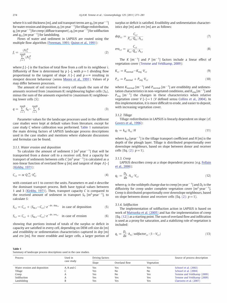
Table 1Summary of landscape process descriptions used in the case studies.

Process Used incase study

Driving factors

Slope

Water erosion and deposition A, B and C YesTillage C YesCreep A YesSolifluction A YesLandsliding B Yes

surplus or deficit is satisfied. Erodibility and sedimentation character-istics dep [m] and ero [m] are as follows:

deps;t =Cs;t

Ps;t⋅Qs;t⋅Λs;tð7Þ

eros;t =Cs;t

Ks;t⋅Qs;t⋅Λs;tð8Þ

The K [m−1] and P [m−1] factors include a linear effect ofvegetation cover (Temme and Veldkamp, 2009):

Ks;t = Knormal−Kveg⋅Vs;t ð9Þ

Ps;t = Pnormal + Pveg⋅Vs;t ð10Þ

where Knormal [m−1] and Pnormal [m−1] are erodibility and sedimen-tation characteristics in non-vegetated conditions, and Kveg [m−1] andPveg [m−1] the changes in these characteristics when relativevegetation cover V [–]=1 (V defined sensu Collins et al., 2004). Inthis implementation, it is more difficult to erode, and easier to deposit,with increasing vegetation cover.

3.1.2. TillageTillage redistribution in LAPSUS is linearly dependent on slope (cf.

Govers et al., 1996):

qT = ktd⋅Λs;t⋅H ð11Þ

where ktd [year−1] is the tillage transport coefficient and H [m] is thedepth of the plough layer. Tillage is distributed proportionally overdownslope neighbours, based on slope between donor and receivercells (Eq. (2): p=1).

3.1.3. CreepLAPSUS describes creep as a slope dependent process (e.g. Follain

et al., 2006):

qC =DE

dx⋅Λs;t⋅Vs;t ð12Þ

where qC is the soildepth change due to creep [m year−1] and DE is thediffusivity for creep under complete vegetation cover [m2 year−1].Creep is distributed proportionally over downslope neighbours, basedon slope between donor and receiver cells (Eq. (2): p=1).

3.1.4. SolifluctionThe implementation of solifluction action in LAPSUS is based on

work of Matsuoka et al. (2005) and has the implementation of creep(Eq. (12)) as a starting point. The sum of overland flow and infiltrationis used as a proxy for saturation, and a stabilizing role of vegetation isincluded:

qs =Ds

dx⋅Λs;t⋅solifactors;t⋅ð1−Vs;tÞ ð13Þ

Source of process description

Overland flow Vegetation

Yes Yes Schoorl et al. (2002)No No Schoorl et al. (2004)No Yes Temme and Veldkamp (2009)Yes Yes Temme and Veldkamp (2009)Yes Yes Claessens et al. (2007)

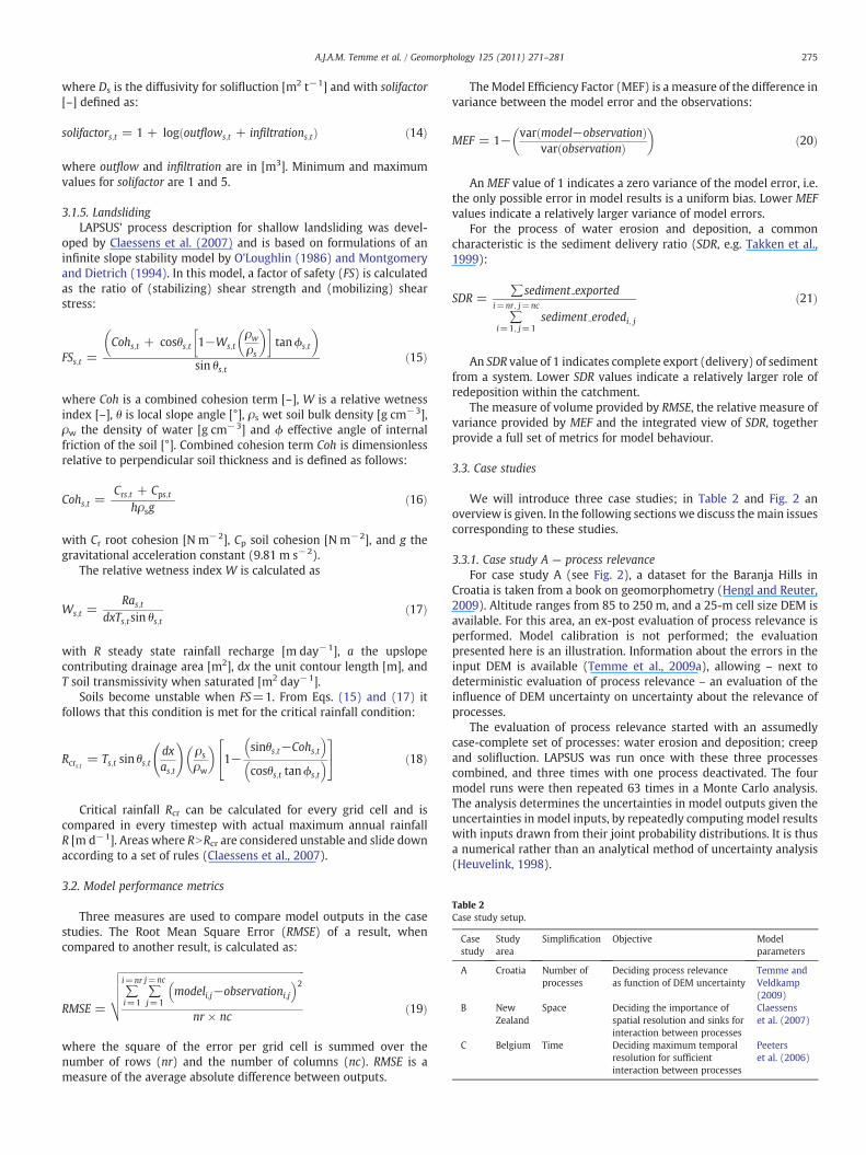
Table 2Case study setup.

Casestudy

Studyarea

Simplification Objective Modelparameters

A Croatia Number ofprocesses

Deciding process relevanceas function of DEM uncertainty

Temme andVeldkamp(2009)

B NewZealand

Space Deciding the importance ofspatial resolution and sinks forinteraction between processes

Claessenset al. (2007)

C Belgium Time Deciding maximum temporalresolution for sufficientinteraction between processes

Peeterset al. (2006)

275A.J.A.M. Temme et al. / Geomorphology 125 (2011) 271–281

where Ds is the diffusivity for solifluction [m2 t−1] and with solifactor[–] defined as:

solifactors;t = 1 + logðoutflows;t + infiltrations;tÞ ð14Þ

where outflow and infiltration are in [m3]. Minimum and maximumvalues for solifactor are 1 and 5.

3.1.5. LandslidingLAPSUS' process description for shallow landsliding was devel-

oped by Claessens et al. (2007) and is based on formulations of aninfinite slope stability model by O'Loughlin (1986) and Montgomeryand Dietrich (1994). In this model, a factor of safety (FS) is calculatedas the ratio of (stabilizing) shear strength and (mobilizing) shearstress:

FSs;t =Cohs;t + cosθs;t 1−Ws;t

ρw

ρs

� �� �tanϕs;t

� �sin θs;t

ð15Þ

where Coh is a combined cohesion term [–], W is a relative wetnessindex [–], θ is local slope angle [°], ρs wet soil bulk density [g cm−3],ρw the density of water [g cm−3] and ϕ effective angle of internalfriction of the soil [°]. Combined cohesion term Coh is dimensionlessrelative to perpendicular soil thickness and is defined as follows:

Cohs;t =Crs;t + Cps;t

hρsgð16Þ

with Cr root cohesion [N m−2], Cp soil cohesion [N m−2], and g thegravitational acceleration constant (9.81 m s−2).

The relative wetness index W is calculated as

Ws;t =Ras;t

dxTs;tsin θs;tð17Þ

with R steady state rainfall recharge [m day−1], a the upslopecontributing drainage area [m2], dx the unit contour length [m], andT soil transmissivity when saturated [m2 day−1].

Soils become unstable when FS=1. From Eqs. (15) and (17) itfollows that this condition is met for the critical rainfall condition:

Rcrs;t = Ts;t sin θs;tdxas;t

!ρs

ρw

� �1−

sinθs;t−Cohs;t� �cosθs;t tanϕs;t

� �24

35 ð18Þ

Critical rainfall Rcr can be calculated for every grid cell and iscompared in every timestep with actual maximum annual rainfallR [m d−1]. Areas where RNRcr are considered unstable and slide downaccording to a set of rules (Claessens et al., 2007).

3.2. Model performance metrics

Three measures are used to compare model outputs in the casestudies. The Root Mean Square Error (RMSE) of a result, whencompared to another result, is calculated as:

RMSE =

ffiffiffiffiffiffiffiffiffiffiffiffiffiffiffiffiffiffiffiffiffiffiffiffiffiffiffiffiffiffiffiffiffiffiffiffiffiffiffiffiffiffiffiffiffiffiffiffiffiffiffiffiffiffiffiffiffiffiffiffiffiffiffiffiffiffiffiffiffiffiffiffiffiffiffiffi∑i=nr

i=1∑j=nc

j=1modeli;j−observationi;j

� �2nr × nc

vuuutð19Þ

where the square of the error per grid cell is summed over thenumber of rows (nr) and the number of columns (nc). RMSE is ameasure of the average absolute difference between outputs.

TheModel Efficiency Factor (MEF) is a measure of the difference invariance between the model error and the observations:

MEF = 1− varðmodel−observationÞvarðobservationÞ

� �ð20Þ

An MEF value of 1 indicates a zero variance of the model error, i.e.the only possible error in model results is a uniform bias. Lower MEFvalues indicate a relatively larger variance of model errors.

For the process of water erosion and deposition, a commoncharacteristic is the sediment delivery ratio (SDR, e.g. Takken et al.,1999):

SDR =∑sediment exported

∑i=nr; j=nc

i=1; j=1sediment erodedi; j

ð21Þ

An SDR value of 1 indicates complete export (delivery) of sedimentfrom a system. Lower SDR values indicate a relatively larger role ofredeposition within the catchment.

The measure of volume provided by RMSE, the relative measure ofvariance provided by MEF and the integrated view of SDR, togetherprovide a full set of metrics for model behaviour.

3.3. Case studies

We will introduce three case studies; in Table 2 and Fig. 2 anoverview is given. In the following sectionswe discuss themain issuescorresponding to these studies.

3.3.1. Case study A — process relevanceFor case study A (see Fig. 2), a dataset for the Baranja Hills in

Croatia is taken from a book on geomorphometry (Hengl and Reuter,2009). Altitude ranges from 85 to 250 m, and a 25-m cell size DEM isavailable. For this area, an ex-post evaluation of process relevance isperformed. Model calibration is not performed; the evaluationpresented here is an illustration. Information about the errors in theinput DEM is available (Temme et al., 2009a), allowing – next todeterministic evaluation of process relevance – an evaluation of theinfluence of DEM uncertainty on uncertainty about the relevance ofprocesses.

The evaluation of process relevance started with an assumedlycase-complete set of processes: water erosion and deposition; creepand solifluction. LAPSUS was run once with these three processescombined, and three times with one process deactivated. The fourmodel runs were then repeated 63 times in a Monte Carlo analysis.The analysis determines the uncertainties in model outputs given theuncertainties in model inputs, by repeatedly computing model resultswith inputs drawn from their joint probability distributions. It is thusa numerical rather than an analytical method of uncertainty analysis(Heuvelink, 1998).

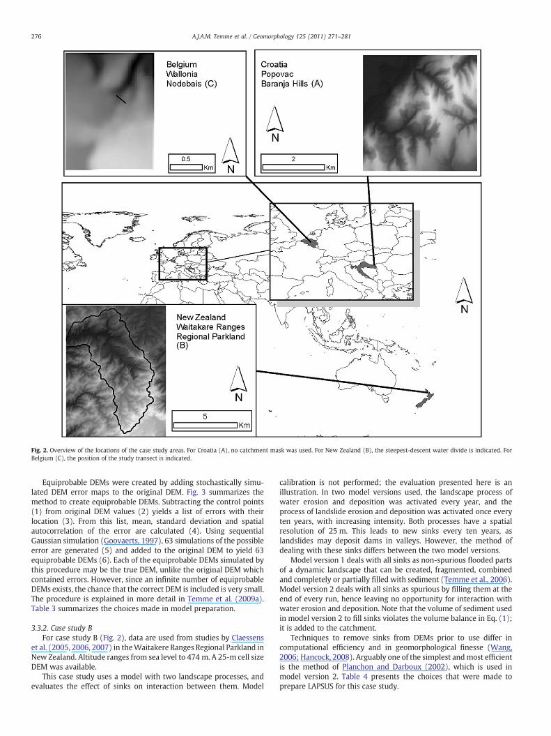
Fig. 2. Overview of the locations of the case study areas. For Croatia (A), no catchment mask was used. For New Zealand (B), the steepest-descent water divide is indicated. ForBelgium (C), the position of the study transect is indicated.

276 A.J.A.M. Temme et al. / Geomorphology 125 (2011) 271–281

Equiprobable DEMs were created by adding stochastically simu-lated DEM error maps to the original DEM. Fig. 3 summarizes themethod to create equiprobable DEMs. Subtracting the control points(1) from original DEM values (2) yields a list of errors with theirlocation (3). From this list, mean, standard deviation and spatialautocorrelation of the error are calculated (4). Using sequentialGaussian simulation (Goovaerts, 1997), 63 simulations of the possibleerror are generated (5) and added to the original DEM to yield 63equiprobable DEMs (6). Each of the equiprobable DEMs simulated bythis procedure may be the true DEM, unlike the original DEM whichcontained errors. However, since an infinite number of equiprobableDEMs exists, the chance that the correct DEM is included is very small.The procedure is explained in more detail in Temme et al. (2009a).Table 3 summarizes the choices made in model preparation.

3.3.2. Case study BFor case study B (Fig. 2), data are used from studies by Claessens

et al. (2005, 2006, 2007) in theWaitakere Ranges Regional Parkland inNew Zealand. Altitude ranges from sea level to 474 m. A 25-m cell sizeDEM was available.

This case study uses a model with two landscape processes, andevaluates the effect of sinks on interaction between them. Model

calibration is not performed; the evaluation presented here is anillustration. In two model versions used, the landscape process ofwater erosion and deposition was activated every year, and theprocess of landslide erosion and deposition was activated once everyten years, with increasing intensity. Both processes have a spatialresolution of 25 m. This leads to new sinks every ten years, aslandslides may deposit dams in valleys. However, the method ofdealing with these sinks differs between the two model versions.

Model version 1 deals with all sinks as non-spurious flooded partsof a dynamic landscape that can be created, fragmented, combinedand completely or partially filled with sediment (Temme et al., 2006).Model version 2 deals with all sinks as spurious by filling them at theend of every run, hence leaving no opportunity for interaction withwater erosion and deposition. Note that the volume of sediment usedin model version 2 to fill sinks violates the volume balance in Eq. (1);it is added to the catchment.

Techniques to remove sinks from DEMs prior to use differ incomputational efficiency and in geomorphological finesse (Wang,2006; Hancock, 2008). Arguably one of the simplest andmost efficientis the method of Planchon and Darboux (2002), which is used inmodel version 2. Table 4 presents the choices that were made toprepare LAPSUS for this case study.

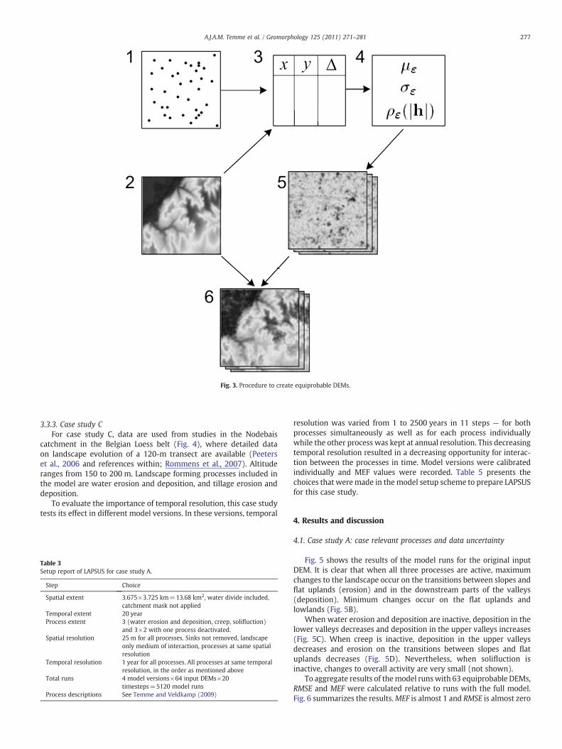
Fig. 3. Procedure to create equiprobable DEMs.

277A.J.A.M. Temme et al. / Geomorphology 125 (2011) 271–281

3.3.3. Case study CFor case study C, data are used from studies in the Nodebais

catchment in the Belgian Loess belt (Fig. 4), where detailed dataon landscape evolution of a 120-m transect are available (Peeterset al., 2006 and references within; Rommens et al., 2007). Altituderanges from 150 to 200 m. Landscape forming processes included inthe model are water erosion and deposition, and tillage erosion anddeposition.

To evaluate the importance of temporal resolution, this case studytests its effect in different model versions. In these versions, temporal

Table 3Setup report of LAPSUS for case study A.

Step Choice

Spatial extent 3.675×3.725 km=13.68 km2, water divide included,catchment mask not applied

Temporal extent 20 yearProcess extent 3 (water erosion and deposition, creep, solifluction)

and 3×2 with one process deactivated.Spatial resolution 25 m for all processes. Sinks not removed, landscape

only medium of interaction, processes at same spatialresolution

Temporal resolution 1 year for all processes. All processes at same temporalresolution, in the order as mentioned above

Total runs 4 model versions×64 input DEMs×20timesteps=5120 model runs

Process descriptions See Temme and Veldkamp (2009)

resolution was varied from 1 to 2500 years in 11 steps — for bothprocesses simultaneously as well as for each process individuallywhile the other process was kept at annual resolution. This decreasingtemporal resolution resulted in a decreasing opportunity for interac-tion between the processes in time. Model versions were calibratedindividually and MEF values were recorded. Table 5 presents thechoices that weremade in themodel setup scheme to prepare LAPSUSfor this case study.

4. Results and discussion

4.1. Case study A: case relevant processes and data uncertainty

Fig. 5 shows the results of the model runs for the original inputDEM. It is clear that when all three processes are active, maximumchanges to the landscape occur on the transitions between slopes andflat uplands (erosion) and in the downstream parts of the valleys(deposition). Minimum changes occur on the flat uplands andlowlands (Fig. 5B).

When water erosion and deposition are inactive, deposition in thelower valleys decreases and deposition in the upper valleys increases(Fig. 5C). When creep is inactive, deposition in the upper valleysdecreases and erosion on the transitions between slopes and flatuplands decreases (Fig. 5D). Nevertheless, when solifluction isinactive, changes to overall activity are very small (not shown).

To aggregate results of themodel runswith 63 equiprobable DEMs,RMSE and MEF were calculated relative to runs with the full model.Fig. 6 summarizes the results.MEF is almost 1 and RMSE is almost zero

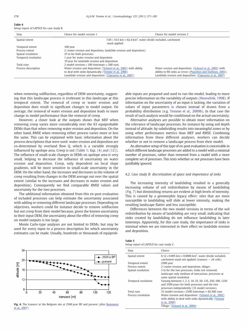
Table 4Setup report of LAPSUS for case study B.

Step Choice for model version 1 Choice for model version 2

Spatial extent 7.85×10.5 km=82.4 km2, water divide included, catchmentmask applied

Temporal extent 100 yearProcess extent 2 (water erosion and deposition, landslide erosion and deposition)Spatial resolution 25 m for both processesTemporal resolution 1 year for water erosion and deposition

10 year for landslide erosion and depositionTotal runs 2 model versions×100 timesteps=200 runsProcess description Water erosion and deposition: (Schoorl et al., 2002) with ability

to deal with sinks dynamically (Temme et al., 2006)Landslide erosion and deposition: (Claessens et al., 2007)

Water erosion and deposition: (Schoorl et al., 2002) withability to fill sinks as errors (Planchon and Darboux, 2002).Landslide erosion and deposition: (Claessens et al., 2007)

278 A.J.A.M. Temme et al. / Geomorphology 125 (2011) 271–281

when removing solifluction, regardless of DEM uncertainty, suggest-ing that this landscape process is irrelevant in this landscape at thistemporal extent. The removal of creep or water erosion anddeposition does result in significant changes in model output. Onaverage, the removal of water erosion and deposition leads to morechange in model performance than the removal of creep.

However, a closer look at the outputs shows that MEF whenremoving creep varies more considerably over the 63 equiprobableDEMs than that when removing water erosion and deposition. On theother hand, RMSE when removing either process varies more or lessthe same. This can be explained with basic information about theprocess descriptions that were used: water erosion and deposition areco-determined by overland flow Q, which is a variable stronglyinfluenced by upslope area. Creep is not (Table 1; Eqs. (4) and (12)).The influence of small-scale changes in DEMs on upslope area is verysmall, helping to decrease the influence of uncertainty on watererosion and deposition. Creep, only dependent on local slopegradients, will be more sensitive to small-scale uncertainty in theDEM. On the other hand, the increases and decreases in the volume ofcreep resulting from changes in the DEM average out over the spatialextent (similar to the increases and decreases in water erosion anddeposition). Consequently we find comparable RMSE values anduncertainty for the two processes.

The additional information obtained from this ex-post evaluationof included processes can help estimate the uncertainty associatedwith adding or removing different landscape processes. Depending onobjectives, workers could for instance decide to remove solifluctionbut not creep from their model because, given the known uncertaintyin their input DEM, the uncertainty about the effect of removing creepon model outputs is too large.

Monte Carlo-type analyses are not limited to DEMs, but may beused for every input to a process description for which uncertaintyestimates can be made. Usually, hundreds or thousands of equiprob-

Fig. 4. The transect at the Belgium site at 2500 year BP and present (after Rommenset al., 2007).

able inputs are prepared and used to run the model, leading to moreprecise information on the variability of outputs (Heuvelink, 1998). Ifinformation on the uncertainty of an input is lacking, the variation ofvalues of input parameters is chosen instead of drawn from aprobability distribution (e.g. Temme et al., 2009b). In that case theresult of such analysis would be conditional on the actual uncertainty.

Alternative analyses are possible to obtain more information onthe relevance of landscape processes, for instance by using soil depthinstead of altitude, by subdividing results into meaningful zones or byusing other performance metrics than MEF and RMSE. Combininginformation from these different analyses, workers can decidewhether or not to remove a landscape process from their model.

An alternative setup of this type of ex-post evaluation is conceivable inwhich different landscape processes are added to amodel with aminimalnumber of processes, rather than removed from a model with a morecomplete set of processes. This tests whether or not processes have beenjustifiably ignored.

4.2. Case study B: discretization of space and importance of sinks

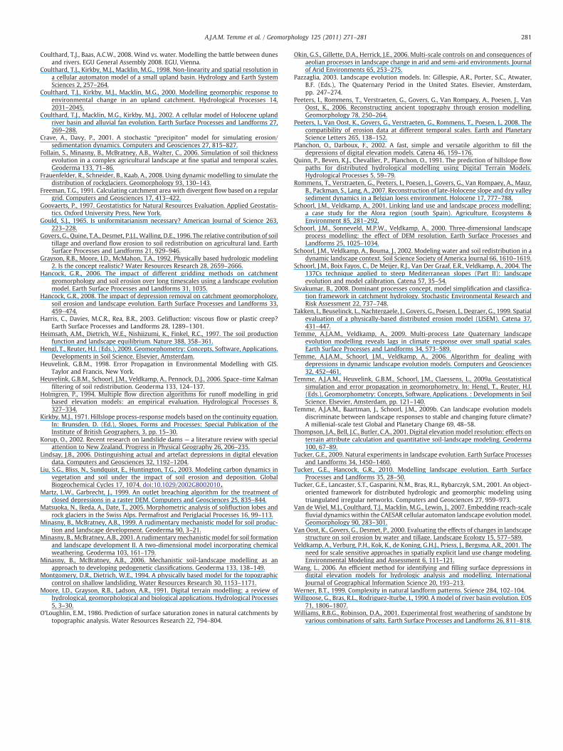
The increasing intensity of landsliding resulted in a generallyincreasing volume of soil redistribution by means of landsliding(Fig. 7) but diminishing returns are evident at high levels of intensity.This is caused by a geomorphic legacy effect: sites that are moresusceptible to landsliding will slide at lower intensity, making theresulting landscape flatter and less susceptible.

Differences between the two model versions in terms of the soilredistribution by means of landsliding are very small, indicating thatsinks created by landsliding do not influence landsliding in latertimesteps. Apparently, for this case study, the importance of sinks isminimal when we are interested in their effect on landslide erosionand deposition.

Table 5Setup report of LAPSUS for case study C.

Step Choice

Spatial extent 0.12×0.005 km=0.0006 km2, water divide included,catchment mask not applied (transect — 24 cells)

Temporal extent 2500 yearProcess extent 2 (water erosion and deposition, tillage)Spatial resolution 5 m for the two processes. Sinks not removed,

landscape only medium of interaction, processes atsame spatial resolution

Temporal resolution Varying between 1, 2, 5, 10, 25, 50, 125, 250, 500, 1250and 2500 years for both processes and the twoprocesses independently (33 model versions).

Total runs 33 model versions×2500 timesteps=82,500 runsProcess resolution Water erosion and deposition: (Schoorl et al., 2002)

with ability to deal with sinks dynamically (Temmeet al., 2006)Tillage: (Schoorl et al., 2004)

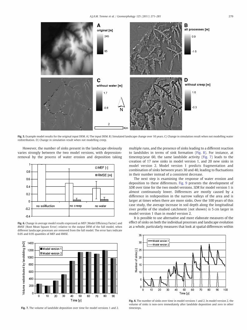
Fig. 5. Example model results for the original input DEM. A) The input DEM. B) Simulated landscape change over 10 years. C) Change in simulation result when not modelling waterredistribution. D) Change in simulation result when not modelling creep.

279A.J.A.M. Temme et al. / Geomorphology 125 (2011) 271–281

However, the number of sinks present in the landscape obviouslyvaries strongly between the two model versions, with depression-removal by the process of water erosion and deposition taking

Fig. 6. Change in average model results expressed asMEF (Model Efficiency Factor) andRMSE (Root Mean Square Error) relative to the output DEM of the full model, whendifferent landscape processes are removed from the full model. The error bars indicate0.05 and 0.95 quantiles of MEF and RMSE.

Fig. 7. The volume of landslide deposition over time for model versions 1 and 2.

multiple runs, and the presence of sinks leading to a different reactionto landslides in terms of sink formation (Fig. 8). For instance, attimestep/year 60, the same landslide activity (Fig. 7) leads to thecreation of 17 new sinks in model version 1, and 20 new sinks inmodel version 2. Model version 1 predicts fragmentation andcombination of sinks between years 30 and 40, leading to fluctuationsin their number instead of a consistent decrease.

The next step is examining the response of water erosion anddeposition to these differences. Fig. 9 presents the development ofSDR over time for the two model versions. SDR for model version 1 isalmost continuously lower. Differences are mostly caused by adifference in redeposition in the narrow valleys of the area and islarger at times when there are more sinks. Over the 100 years of thiscase study, the average increase in soil depth along the longitudinalriver profile of the studied catchment (not shown) is 5 cm larger inmodel version 1 than in model version 2.

It is possible to use alternative and more elaborate measures of theeffect of sinks on both the individual processes and landscape evolutionas a whole, particularly measures that look at spatial differences within

Fig. 8. The number of sinks over time in model versions 1 and 2. In model version 2, thevolume of sinks is non-zero immediately after landslide deposition and zero in othertimesteps.

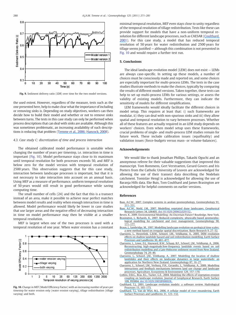
Fig. 9. Sediment delivery ratio (SDR) over time for the two model versions.

280 A.J.A.M. Temme et al. / Geomorphology 125 (2011) 271–281

the used extent. However, regardless of the measure, tests such as theone presented here, help tomake clearwhat the importance of includingor removing sinks is. Depending on study objectives, workers can thendecide how to build their model and whether or not to remove sinksbetween turns. The tests in this case study can only be performed whenprocess descriptions that can deal with sinks are available. Although thiswas sometimes problematic, an increasing availability of such descrip-tions is reducing that problem (Temme et al., 2006; Hancock, 2008).

4.3. Case study C: discretization of time and process interaction

The obtained calibrated model performance is unstable whenchanging the number of years per timestep, i.e. interaction in time isimportant (Fig. 10). Model performance stays close to its maximumuntil temporal resolution for both processes exceeds 50, and MEF isbelow zero for the model version with temporal resolution of2500 years. This observation suggests that for this case study,interaction between landscape processes is important, but that it isnot necessary to take interaction into account on an annual basis.UsingMEF as a measure of performance, uniform temporal resolutionof 50 years would still result in good performance while savingcomputing time.

The small number of cells (24) and the fact that this is a transectinstead of an area, make it possible to achieve near perfect matchesbetween model results and reality when enough interaction in time isallowed. Model performance would likely be lower in case studiesthat use larger areas and the negative effect of decreasing interactionin time on model performance may then be visible at a smallertemporal resolution.

MEF is largest when one of the two processes is used with atemporal resolution of one year. When water erosion has a constant

Fig. 10. Change inMEF (Model Efficiency Factor) with an increasing number of years pertimestep for water erosion only (water erosion varying), tillage redistribution (tillagevarying) and both.

minimal temporal resolution,MEF even stays close to unity regardlessof the temporal resolution of tillage redistribution. Tests like these canprovide support for models that have a non-uniform temporal re-solution for different landscape processes, such as CAESAR (Coulthard,2001). For this case study, a model that has reduced temporalresolution of 50 years for water redistribution and 2500 years fortillage seems justified— although this combination is not presented inFig. 10 and would require a further test run.

5. Conclusions

The ideal landscape evolution model (LEM) does not exist — LEMsare always case-specific. In setting up these models, a number ofchoices must be consciously made and reported on, and some choicesare especially important for multi-process LEMs. The tests in the casestudies illustratemethods tomake the choices, typically by comparingthe results of different model versions. Taken together, these tests canhelp to set up multi-process LEMs for various settings, or assess thevalidity of existing models. Furthermore, they can indicate thesensitivity of models for different simplifications.

LEM frameworks would ideally facilitate the different choices inmodel setup. This requires at least that: i) such frameworks aremodular, ii) they can deal with non-spurious sinks and iii) they allowspatial and temporal resolution to vary between processes. Whetherall of these features are actually required in an LEM study depends onworkers' choices. Even when model setup uses these frameworks,crucial problems of single- and multi-process LEM studies remain forfuture work. These include calibration issues (equifinality) andvalidation issues (force-budgets versus mass- or volume-balances).

Acknowledgements

We would like to thank Jonathan Phillips, Takashi Oguchi and ananonymous referee for their valuable suggestions that improved thismanuscript. Tom Rommens, Gert Verstraeten, Gerard Govers and IrisPeeters from the Catholic University of Leuven are acknowledged forallowing the use of their transect data describing the Nodebaiscatchment. Tomislav Hengl is acknowledged for allowing the use ofBaranja Hills data. Eke Buis, Tom Coulthard and James Brasington areacknowledged for helpful comments on earlier versions.

References

Baas, A.C.W., 2007. Complex systems in aeolian geomorphology. Geomorphology 91,311–331.

Baas, A.C.W., Nield, J.M., 2007. Modelling vegetated dune landscapes. GeophysicalResearch Letters 34, L06405. doi:10.1029/2006GL029152.

Beven, K., 2009. Environmental Modelling: An Uncertain Future? Routledge, New York.Brasington, J., Richards, K., 2007. Reduced-complexity, physically-based geomorpho-

logical modelling for catchment and river management. Geomorphology 90,171–177.

Braun, J., Sambridge, M., 1997. Modelling landscape evolution on geological time scales:a new method based on irregular spatial discretization. Basin Research 9, 27–52.

Claessens, L., Heuvelink, G.B.M., Schoorl, J.M., Veldkamp, A., 2005. DEM resolutioneffects on shallow landslide hazard and soil redistribution modelling. Earth SurfaceProcesses and Landforms 30, 461–477.

Claessens, L., Lowe, D.J., Hayward, B.W., Schaap, B.F., Schoorl, J.M., Veldkamp, A., 2006.Reconstructing high-magnitude/low-frequency landslide events based on soilredistribution modelling and a Late-Holocene sediment record from New Zealand.Geomorphology 74, 29–49.

Claessens, L., Schoorl, J.M., Veldkamp, A., 2007. Modelling the location of shallowlandslides and their effects on landscape dynamics in large watersheds: anapplication for Northern New Zealand. Geomorphology 87, 16–27.

Claessens, L., Schoorl, J.M., Verburg, P.H., Geraedts, L., Veldkamp, A., 2009. Modellinginteractions and feedback mechanisms between land use change and landscapeprocesses. Agriculture, Ecosystems & Environment 129, 157–170.

Collins, D.B.G., Bras, R.L., Tucker, G.E., 2004. Modeling the effects of vegetation-erosioncoupling on landscape evolution. Journal of Geophysical Research, Earth Surface109, F03004. doi:10.1029/2003JF000028.

Coulthard, T.J., 2001. Landscape evolution models: a software review. HydrologicalProcesses 15, 165–173.

Coulthard, T.J., Van de Wiel, M.J., 2006. A cellular model of river meandering. EarthSurface Processes and Landforms 31, 123–132.

281A.J.A.M. Temme et al. / Geomorphology 125 (2011) 271–281

Coulthard, T.J., Baas, A.C.W., 2008. Wind vs. water. Modelling the battle between dunesand rivers. EGU General Assembly 2008. EGU, Vienna.

Coulthard, T.J., Kirkby, M.J., Macklin, M.G., 1998. Non-linearity and spatial resolution ina cellular automaton model of a small upland basin. Hydrology and Earth SystemSciences 2, 257–264.

Coulthard, T.J., Kirkby, M.J., Macklin, M.G., 2000. Modelling geomorphic response toenvironmental change in an upland catchment. Hydrological Processes 14,2031–2045.

Coulthard, T.J., Macklin, M.G., Kirkby, M.J., 2002. A cellular model of Holocene uplandriver basin and alluvial fan evolution. Earth Surface Processes and Landforms 27,269–288.

Crave, A., Davy, P., 2001. A stochastic “precipiton” model for simulating erosion/sedimentation dynamics. Computers and Geosciences 27, 815–827.

Follain, S., Minasny, B., McBratney, A.B., Walter, C., 2006. Simulation of soil thicknessevolution in a complex agricultural landscape at fine spatial and temporal scales.Geoderma 133, 71–86.

Frauenfelder, R., Schneider, B., Kaab, A., 2008. Using dynamic modelling to simulate thedistribution of rockglaciers. Geomorphology 93, 130–143.

Freeman, T.G., 1991. Calculating catchment area with divergent flow based on a regulargrid. Computers and Geosciences 17, 413–422.

Goovaerts, P., 1997. Geostatistics for Natural Resources Evaluation. Applied Geostatis-tics. Oxford University Press, New York.

Gould, S.J., 1965. Is uniformitarianism necessary? American Journal of Science 263,223–228.

Govers, G., Quine, T.A., Desmet, P.J.J., Walling, D.E., 1996. The relative contribution of soiltillage and overland flow erosion to soil redistribution on agricultural land. EarthSurface Processes and Landforms 21, 929–946.

Grayson, R.B., Moore, I.D., McMahon, T.A., 1992. Physically based hydrologic modeling2. Is the concept realistic? Water Resources Research 28, 2659–2666.

Hancock, G.R., 2006. The impact of different gridding methods on catchmentgeomorphology and soil erosion over long timescales using a landscape evolutionmodel. Earth Surface Processes and Landforms 31, 1035.

Hancock, G.R., 2008. The impact of depression removal on catchment geomorphology,soil erosion and landscape evolution. Earth Surface Processes and Landforms 33,459–474.

Harris, C., Davies, M.C.R., Rea, B.R., 2003. Gelifluction: viscous flow or plastic creep?Earth Surface Processes and Landforms 28, 1289–1301.

Heimsath, A.M., Dietrich, W.E., Nishiizumi, K., Finkel, R.C., 1997. The soil productionfunction and landscape equilibrium. Nature 388, 358–361.

Hengl, T., Reuter, H.I. (Eds.), 2009. Geomorphometry: Concepts, Software, Applications.Developments in Soil Science. Elsevier, Amsterdam.

Heuvelink, G.B.M., 1998. Error Propagation in Environmental Modelling with GIS.Taylor and Francis, New York.

Heuvelink, G.B.M., Schoorl, J.M., Veldkamp, A., Pennock, D.J., 2006. Space–time Kalmanfiltering of soil redistribution. Geoderma 133, 124–137.

Holmgren, P., 1994. Multiple flow direction algorithms for runoff modelling in gridbased elevation models: an empirical evaluation. Hydrological Processes 8,327–334.

Kirkby, M.J., 1971. Hillslope process-response models based on the continuity equation.In: Brunsden, D. (Ed.), Slopes, Forms and Processes: Special Publication of theInstitute of British Geographers, 3, pp. 15–30.

Korup, O., 2002. Recent research on landslide dams — a literature review with specialattention to New Zealand. Progress in Physical Geography 26, 206–235.

Lindsay, J.B., 2006. Distinguishing actual and artefact depressions in digital elevationdata. Computers and Geosciences 32, 1192–1204.

Liu, S.G., Bliss, N., Sundquist, E., Huntington, T.G., 2003. Modeling carbon dynamics invegetation and soil under the impact of soil erosion and deposition. GlobalBiogeochemical Cycles 17, 1074. doi:10.1029/2002GB002010.

Martz, L.W., Garbrecht, J., 1999. An outlet breaching algorithm for the treatment ofclosed depressions in a raster DEM. Computers and Geosciences 25, 835–844.

Matsuoka, N., Ikeda, A., Date, T., 2005. Morphometric analysis of solifluction lobes androck glaciers in the Swiss Alps. Permafrost and Periglacial Processes 16, 99–113.

Minasny, B., McBratney, A.B., 1999. A rudimentary mechanistic model for soil produc-tion and landscape development. Geoderma 90, 3–21.

Minasny, B., McBratney, A.B., 2001. A rudimentary mechanistic model for soil formationand landscape development II. A two-dimensional model incorporating chemicalweathering. Geoderma 103, 161–179.

Minasny, B., McBratney, A.B., 2006. Mechanistic soil-landscape modelling as anapproach to developing pedogenetic classifications. Geoderma 133, 138–149.

Montgomery, D.R., Dietrich, W.E., 1994. A physically based model for the topographiccontrol on shallow landsliding. Water Resources Research 30, 1153–1171.

Moore, I.D., Grayson, R.B., Ladson, A.R., 1991. Digital terrain modelling; a review ofhydrological, geomorphological and biological applications. Hydrological Processes5, 3–30.

O'Loughlin, E.M., 1986. Prediction of surface saturation zones in natural catchments bytopographic analysis. Water Resources Research 22, 794–804.

Okin, G.S., Gillette, D.A., Herrick, J.E., 2006. Multi-scale controls on and consequences ofaeolian processes in landscape change in arid and semi-arid environments. Journalof Arid Environments 65, 253–275.

Pazzaglia, 2003. Landscape evolution models. In: Gillespie, A.R., Porter, S.C., Atwater,B.F. (Eds.), The Quaternary Period in the United States. Elsevier, Amsterdam,pp. 247–274.

Peeters, I., Rommens, T., Verstraeten, G., Govers, G., Van Rompaey, A., Poesen, J., VanOost, K., 2006. Reconstructing ancient topography through erosion modelling.Geomorphology 78, 250–264.

Peeters, I., Van Oost, K., Govers, G., Verstraeten, G., Rommens, T., Poesen, J., 2008. Thecompatibility of erosion data at different temporal scales. Earth and PlanetaryScience Letters 265, 138–152.

Planchon, O., Darboux, F., 2002. A fast, simple and versatile algorithm to fill thedepressions of digital elevation models. Catena 46, 159–176.

Quinn, P., Beven, K.J., Chevallier, P., Planchon, O., 1991. The prediction of hillslope flowpaths for distributed hydrological modelling using Digital Terrain Models.Hydrological Processes 5, 59–79.

Rommens, T., Verstraeten, G., Peeters, I., Poesen, J., Govers, G., Van Rompaey, A., Mauz,B., Packman, S., Lang, A., 2007. Reconstruction of late-Holocene slope and dry valleysediment dynamics in a Belgian loess environment. Holocene 17, 777–788.

Schoorl, J.M., Veldkamp, A., 2001. Linking land use and landscape process modelling:a case study for the Alora region (south Spain). Agriculture, Ecosystems &Environment 85, 281–292.

Schoorl, J.M., Sonneveld, M.P.W., Veldkamp, A., 2000. Three-dimensional landscapeprocess modelling: the effect of DEM resolution. Earth Surface Processes andLandforms 25, 1025–1034.

Schoorl, J.M., Veldkamp, A., Bouma, J., 2002. Modeling water and soil redistribution in adynamic landscape context. Soil Science Society of America Journal 66, 1610–1619.

Schoorl, J.M., Boix Fayos, C., De Meijer, R.J., Van Der Graaf, E.R., Veldkamp, A., 2004. The137Cs technique applied to steep Mediterranean slopes (Part II): landscapeevolution and model calibration. Catena 57, 35–54.

Sivakumar, B., 2008. Dominant processes concept, model simplification and classifica-tion framework in catchment hydrology. Stochastic Environmental Research andRisk Assessment 22, 737–748.

Takken, I., Beuselinck, L., Nachtergaele, J., Govers, G., Poesen, J., Degraer, G., 1999. Spatialevaluation of a physically-based distributed erosion model (LISEM). Catena 37,431–447.

Temme, A.J.A.M., Veldkamp, A., 2009. Multi-process Late Quaternary landscapeevolution modelling reveals lags in climate response over small spatial scales.Earth Surface Processes and Landforms 34, 573–589.

Temme, A.J.A.M., Schoorl, J.M., Veldkamp, A., 2006. Algorithm for dealing withdepressions in dynamic landscape evolution models. Computers and Geosciences32, 452–461.

Temme, A.J.A.M., Heuvelink, G.B.M., Schoorl, J.M., Claessens, L., 2009a. Geostatisticalsimulation and error propagation in geomorphometry. In: Hengl, T., Reuter, H.I.(Eds.), Geomorphometry: Concepts, Software, Applications. : Developments in SoilScience. Elsevier, Amsterdam, pp. 121–140.

Temme, A.J.A.M., Baartman, J., Schoorl, J.M., 2009b. Can landscape evolution modelsdiscriminate between landscape responses to stable and changing future climate?A millenial-scale test Global and Planetary Change 69, 48–58.

Thompson, J.A., Bell, J.C., Butler, C.A., 2001. Digital elevationmodel resolution: effects onterrain attribute calculation and quantitative soil-landscape modeling. Geoderma100, 67–89.

Tucker, G.E., 2009. Natural experiments in landscape evolution. Earth Surface Processesand Landforms 34, 1450–1460.

Tucker, G.E., Hancock, G.R., 2010. Modelling landscape evolution. Earth SurfaceProcesses and Landforms 35, 28–50.

Tucker, G.E., Lancaster, S.T., Gasparini, N.M., Bras, R.L., Rybarczyk, S.M., 2001. An object-oriented framework for distributed hydrologic and geomorphic modeling usingtriangulated irregular networks. Computers and Geosciences 27, 959–973.

Van de Wiel, M.J., Coulthard, T.J., Macklin, M.G., Lewin, J., 2007. Embedding reach-scalefluvial dynamics within the CAESAR cellular automaton landscape evolutionmodel.Geomorphology 90, 283–301.

Van Oost, K., Govers, G., Desmet, P., 2000. Evaluating the effects of changes in landscapestructure on soil erosion by water and tillage. Landscape Ecology 15, 577–589.

Veldkamp, A., Verburg, P.H., Kok, K., de Koning, G.H.J., Priess, J., Bergsma, A.R., 2001. Theneed for scale sensitive approaches in spatially explicit land use change modeling.Environmental Modeling and Assessment 6, 111–121.

Wang, L., 2006. An efficient method for identifying and filling surface depressions indigital elevation models for hydrologic analysis and modelling. InternationalJournal of Geographical Information Science 20, 193–213.

Werner, B.T., 1999. Complexity in natural landform patterns. Science 284, 102–104.Willgoose, G., Bras, R.L., Rodriguez-Iturbe, I., 1990. Amodel of river basin evolution. EOS

71, 1806–1807.Williams, R.B.G., Robinson, D.A., 2001. Experimental frost weathering of sandstone by

various combinations of salts. Earth Surface Processes and Landforms 26, 811–818.