EVS28 International Electric Vehicle Symposium and Exhibition 1 EVS28 KINTEX, Korea, May 3-6, 2015 EV (Electric Vehicle) Fleet Size and Composition Optimization based on Demand Satisfaction and Total Costs Minimization Taekwan Yoon 1 , Chris R. Cherry 2 1 LG CNS (corresponding author), Seoul, KOREA, [email protected] 2 University of Tennessee, Knoxville, TN, USA, [email protected] Abstract Managing a fleet efficiently to addresses demand within cost constraints is a challenge. Mismatched fleet size and demand can create suboptimal budget allocations and inconvenience users. To address this problem, many studies have been conducted around heterogeneous fleet optimization. That research has not included an examination of different vehicle types with travel distance constraints. This study focuses on optimizing the University of Tennessee (UT) motor pool which has a heterogeneous fleet that includes EVs with a travel distance and recharge time constraint. After assessing UT motor pool trip patterns, a Queuing model was used to estimate the maximum number of each vehicle type needed to minimize the expected customer wait time to near zero. The break-even point is used for optimization model to constrain the minimum number of years that electric vehicles should be operated under the no subsidy assumption. The models are very flexible and can be applied to a wide variety of fleet optimization problems. It can help fleet managers make decisions about fleet size and EV adoption. In the case of UT’s motor pool, the results show that the fleet has surplus vehicles. In addition to reducing the number of vehicles, total fleet costs could be minimized by using electric vehicles for all trips less than 100 miles. Keywords: Electric vehicle, Fleet optimization, Motor pool, Break-even point, Queuing theory 1 Introduction Managing a fleet efficiently to addresses demand within cost constraints is a challenge. A fleet management program balances many objectives including driver management, speed management, fuel management, route management, fleet size and composition management. If those objectives are not balanced, users may be inconvenienced and total fleet costs could be suboptimal. This study examines fleet size and composition management, with a focus on the role of electric vehicles (EVs) in corporate passenger car fleets. Several earlier studies have examined fleet size and composition management, but none have addressed the unique operational characteristics of EVs in fleet optimization. Recently, EVs have emerged as an alternative fuel vehicle that can address many sustainability challenges. With low emissions and lower operating costs (fuel and maintenance) than conventional vehicles (CVs), they are becoming more popular in commercial uses (Funk and Rabl 1999). This is despite the vehicles’ significantly different performance characteristics and fixed costs, such as purchase price, depreciation, refueling infrastructure, and registration fees. An EV’s purchase price is higher than a CV’s purchase price, but this can be balanced by

Welcome message from author
This document is posted to help you gain knowledge. Please leave a comment to let me know what you think about it! Share it to your friends and learn new things together.
Transcript

EVS28 International Electric Vehicle Symposium and Exhibition 1
EVS28
KINTEX, Korea, May 3-6, 2015
EV (Electric Vehicle) Fleet Size and Composition
Optimization based on Demand Satisfaction
and Total Costs Minimization Taekwan Yoon
1, Chris R. Cherry
2
1LG CNS (corresponding author), Seoul, KOREA, [email protected] 2University of Tennessee, Knoxville, TN, USA, [email protected]
Abstract
Managing a fleet efficiently to addresses demand within cost constraints is a challenge. Mismatched fleet
size and demand can create suboptimal budget allocations and inconvenience users. To address this
problem, many studies have been conducted around heterogeneous fleet optimization. That research has not
included an examination of different vehicle types with travel distance constraints. This study focuses on
optimizing the University of Tennessee (UT) motor pool which has a heterogeneous fleet that includes EVs
with a travel distance and recharge time constraint. After assessing UT motor pool trip patterns, a Queuing
model was used to estimate the maximum number of each vehicle type needed to minimize the expected
customer wait time to near zero. The break-even point is used for optimization model to constrain the
minimum number of years that electric vehicles should be operated under the no subsidy assumption. The
models are very flexible and can be applied to a wide variety of fleet optimization problems. It can help
fleet managers make decisions about fleet size and EV adoption. In the case of UT’s motor pool, the results
show that the fleet has surplus vehicles. In addition to reducing the number of vehicles, total fleet costs
could be minimized by using electric vehicles for all trips less than 100 miles.
Keywords: Electric vehicle, Fleet optimization, Motor pool, Break-even point, Queuing theory
1 Introduction Managing a fleet efficiently to addresses demand
within cost constraints is a challenge. A fleet
management program balances many objectives
including driver management, speed
management, fuel management, route
management, fleet size and composition
management. If those objectives are not balanced,
users may be inconvenienced and total fleet costs
could be suboptimal. This study examines fleet
size and composition management, with a focus
on the role of electric vehicles (EVs) in corporate passenger car fleets. Several earlier studies have
examined fleet size and composition management,
but none have addressed the unique operational
characteristics of EVs in fleet optimization.
Recently, EVs have emerged as an alternative fuel
vehicle that can address many sustainability
challenges. With low emissions and lower
operating costs (fuel and maintenance) than
conventional vehicles (CVs), they are becoming
more popular in commercial uses (Funk and Rabl
1999). This is despite the vehicles’ significantly
different performance characteristics and fixed
costs, such as purchase price, depreciation,
refueling infrastructure, and registration fees. An
EV’s purchase price is higher than a CV’s
purchase price, but this can be balanced by
EVS28 International Electric Vehicle Symposium and Exhibition 2
variable costs like fuel, insurance, and
maintenance costs. An EV’s variable costs are
significantly lower than a CV’s. Beyond costs,
EVs’ commercial success is impacted by two
additional characteristics: their short driving
distance and long refueling (recharging) time.
EVs need to be driven often for the fuel cost
savings to overcome the high fixed costs. Range
and recharging time constrain an EV owner’s
ability to maximize EV use and economic
performance.
Vehicle fleets offer a unique opportunity to
manage supply and demand by assigning the
appropriate vehicle technology (CV or EV) for
each trip. Despite that, most vehicle fleets
currently rely on gasoline internal combustion
engine vehicles, CVs (Samaras and Meisterling
2008). But EVs could easily be integrated into
existing fleets. First, fleets usually have
centralized parking and dispatch locations that
could readily incorporate an EV charging
infrastructure. Secondly, with customer’s
frequent short trips, EVs could have high
utilization rates. Third, with known trip distance
and duration, managers can appropriately match
vehicle type to individual trips.
This chapter develops an optimization
framework for corporate fleet adoption of EVs,
this includes developing a model for overall fleet
size and the appropriate mix of EVs and CVs.
The chapter focuses on the University of
Tennessee (UT) motor pool, which is located to
Knoxville, Tennessee. UT motor pool serves the
transportation needs of faculty, staff, and
students conducting official business. This study
applies fleet optimization methods to investigate
the trip patterns of UT motor pool and find how
many of those trips are EV compatible.
Optimized fleet size, compositions, and required
operating years are the objective values with cost
constraints in the optimization model.
2 Literature Reviews
2.1 Electric vehicle
The transportation sector has developed plug in
battery EVs and other technologies in
recognition of the importance of fuel
consumption and energy security, economic
efficiency, health concerns, and environmental
impacts (Wirasingha, Schofield et al. 2008). EVs
(defined as battery EVs here) rely solely on
battery power charged through a charging station.
Balancing expensive and heavy battery capacity
requirements with expected range usually results in
commercial EVs with lower driving range than an
equivalent CV (Lester B. Lave 1995).
EVs have existed for more than 150 years (Lixin
2009). Because of production efficiencies and
easily available, cheap fossil fuel, CVs became
widespread through the 20th century. In recent
decades, battery technology improvements have
allowed for improved EV designs. The industry
has developed more energy efficient and less
polluting EVs (Lixin 2009). Using electricity and
without tailpipe emissions, EVs can help reduce
operating costs and fuel consumption (Shiau,
Kaushal et al. 2010). EVs’ popularity can be
attributed to its potential for reducing a country’s
dependence on imported petroleum and its
greenhouse gas (GHG) emissions (Taylor, Maitra
et al. 2009). This GHG reduction holds even when
balancing EVs increased electric consumption that
causes increased pollution from electricity
generating sources (Funk and Rabl 1999). Thus
recent commercialized EVs have been relatively
successful with markets in the United States,
Europe, and China where a new energy vehicle
policy subsidizes EV deployment.
Because costs, driving range, fuel efficiency,
vehicle gross weight, and other factors differ from
EVs to CVs, fleets must precisely determine its
vehicles’ needed specifications and characteristics.
Even though the EVs’ purchase price is higher
than that of gasoline or diesel vehicles, other
variable costs like fuel, maintenance and coupled
with purchase subsidies, the registration with
incentive, insurance, maintenance, repair, and
energy price of EVs are lower than those of CVs.
This study introduces and analyzes one
commercialized EV, the Nissan Leaf, because of
its publically available specification and
performance information. The Nissan Leaf has an
80kW AC synchronous electric motor, a 24kWh
lithium-ion battery, a 3.3kW onboard charger, and
a battery heater. The Environmental Protection
Agency (EPA) LA-4 city cycle laboratory tests
determined it has a driving range of up to 100
miles. Based upon EPA five-cycle tests, using
varying driving conditions and climate controls,
the EPA has rated the Nissan LEAF at a driving
range of 73 miles. EPA MPG equivalent is 106
(city) and 92 (hwy) miles (Nissan USA n.d.). This
study assumes that EV can drive up to 100 miles.
2.2 EV benefits compared to CV
In general, CVs contribute to local air pollution,
noise pollution, water pollution, and other
pollution. Air pollution may cause reduced

EVS28 International Electric Vehicle Symposium and Exhibition 3
visibility, crop losses, material damage, forest
damage, climate change and human health
impacts (Delucchi 2000). CVs emit many kinds
of exhaust pollutants such as particulates,
hydrocarbons, nitrogen oxides (NOx), carbon
monoxide (CO), carbon dioxide (CO2), and other
pollutants. The emissions can either affect the
environment directly through diminished air
quality and climate change or be precursors to
species of concern, which are formed in the
atmosphere. The former includes carbon
monoxide (CO), and the latter includes volatile
organic compounds (VOCs) and nitrogen oxides
(NOx) which are precursors to the photochemical
formation of ozone and PM (Parrish 2006).
Diesel vehicles have different emission
characteristics than gasoline vehicles, e.g., NOx
emission levels are higher for diesel vehicles
(Rexeis and Hausberger 2009).
Older vehicles without advanced pollution
control technology cause a significant amount of
urban emissions. Some argue for an automobile
replacement policy, where old cars need to be
replaced by new ones to prevent continuous use
of inefficient and higher-polluting vehicles. The
retirement program sometimes incentivizes
owners of older vehicles to replace old vehicles
earlier (Dill 2004). Kim et al. (Kim, Keoleian et
al. 2003) suggest that vehicle retirement should
be decided by economic factors such as repair
cost, market price, and scrap price of a used
vehicle.
Previous research (Samaras and Meisterling
2008) concludes that the EVs can reduce 38-41%
of GHG emissions compared to the CVs and 7-
12% of the emissions compared to traditional
hybrids. They find that the EV battery, especially
lithium-ion battery material and production,
accounts for 2-5% of an EV’s life cycle GHG
emissions. They also point out the importance of
using electricity for energy which influences
GHG emissions.
Emission factors for EVs are very sensitive to the
time of recharging, the source of electricity, and
the region an EV is charge (Hadley and
Tsvetkova 2009). Coal (38%) is the largest share
of electricity source followed renewable (20%),
nuclear (17%), natural gas (16%), and oil (9%).
Previous research expected the electricity
production will be almost double by 2020. As
more natural gas and nuclear power plants
replace older coal power plants, this range should
improve (Sims, Rogner et al. 2003).
2.3 Fleet optimization models
This paper builds on previous research to study
how to utilize EVs in vehicle fleets; it develops a
model based on fleet size and composition. The
vehicle routing problem (VRP) serves as a
precursor to the fleet optimization model.
Proposed by Dantzig and Ramser in 1959, the
VRP is a combinatorial optimization and integer
programming approach seeking to service a
number of customers with a fleet of vehicles
(Crevier, Cordeau et al. 2007). Since its inception,
numerous studies have used and developed the
VRP. With several kinds of VRP, this study
divides them into two categories: capacitated
vehicle routing problem (CVRP) (Golden 1988,
Toth and Vigo 2001, Baldacci, Toth et al. 2007,
Crevier, Cordeau et al. 2007, Gendreau, Iori et al.
2008, Golden, Raghavan et al. 2008, Côté and
Potvin 2009, Eksioglu, Vural et al. 2009, Laporte
2009, Thibaut Vidal 2012) and capacitated arc
routing problem (CARP) that improves local
search procedures (Golden and Wong 1981).
Some have focused on heterogeneous mixed fleet
optimization by narrowing down from VRP and
dispatch models. Several studies (Choi and Tcha
2007, Baldacci, Battarra et al. 2008, Baldacci and
Mingozzi 2009, Prins 2009, Brandão 2011, Penna,
Subramanian et al. 2013) have examined the
heterogeneous VRP (HVRP). In the applications of
HVRP, they tried to minimize total cost by
dispatching each vehicle type, defined by its
capacity, a fixed cost, a distance unit, and
availability.
Previous research also developed an optimization
model that minimizes life cycle cost, petroleum
consumption, and GHG emissions for conventional,
hybrid, and plug-in hybrid vehicles under several
scenarios. They concluded that high battery costs,
low gas prices, and high electricity prices
drastically reduced the financial viability of plug-
in EVs (Shiau, Kaushal et al. 2010).
There have been two studies for the University of
Tennessee Motor pool fleet. Even though the data
and information are old, these studies show the UT
motor pool’s history. Early research in 1980 found
that the UT motor pool’s vehicle request rates were
time-dependent and non-stationary Poisson
processes. Over 85% of the trips were five days or
less. Also, the research did regression analysis for
check out duration and distance travelled. It shows
a strong linear relationship with 0.92 R2 (total trip
mileage by length of trip). Service level and fleet
utilization metrics were used to assess the motor
pool’s service capability (Fowler 1980). A different study pointed out that increasing the fleet

EVS28 International Electric Vehicle Symposium and Exhibition 4
reduces the number of unsatisfied requests, but
increases the fixed investment in the motor pool.
Also, they found that the peak for checking out
vehicles is early in the week and that the demand
decreases later in the week. The check out
duration followed an exponential distribution
(Williams and Fowler 1979).
3 Data Analysis
3.1 UT motor pool data description
The UT motor pool was set up in the early
1950’s and stayed relatively small in scale for
over a decade. In 1960’s the University
experienced a sharp enrollment increase and
requests for dispatch vehicles grew rapidly. So a
large number of vehicles were added to the fleet
to satisfy the increasing demand (Fowler 1980).
Over the years many procedures have been
implemented to maintain UT motor pool vehicles.
Users are encouraged to use an on-site fueling
station or a fleet fueling card at participating gas
stations. The vehicles are maintained and
repaired in-house except in cases of severe
damage when the vehicles serviced outside. Any
vehicles older than three years or that have
traveled 80,000 miles, whichever is first, are sold
through public auctions each spring.
This study examines data collected between
March 14, 2011 and February 20, 2012. The fleet
consisted of 95 mid-size gasoline sedans that
made a total of 1,937 trips. The sedans were
2008-2011 Dodge Avengers and 2011 Ford
Fusions. The rated fuel economies (averaged
over 4 model years) ranged from 20 - 22 miles
per gallon (mpg) for city and 28.5 - 30 mpg for
highway. Since only mid-size sedans can be
potentially replaced by EVs such as the Nissan
Leaf, only those fleet data were analyzed.
3.2 Data analysis
To assess the trip patterns of the UT motor pool
vehicles, this study analyzed the times at which
the vehicles were checked out, the distance
traveled, and the destinations from the given data
(Table 1). The median value of checkout duration
and distance traveled are 70 hours (3 days) and
409 miles, respectively.
Around 40% of the total trips are local, meaning
that the destinations were in counties bordering
the UT campus in Knoxville. The destinations of
79% of the trips are within the state of Tennessee.
The longer duration of checkout times reflects
overnight or weekend checkouts. Figure 1 shows
the frequency of the number of vehicles checked
out at a given time. The most frequent number of
simultaneously checked out vehicles is 43 and the
average is 20~25 vehicles. This will be used to
evaluate the model suggested in this chapter.
About 96% of demand is met by 30 vehicles.
Table 1 UT motor pool check-out pattern 85%tile 50%tile 15%tile Max Min Median
Using time
(hours)
113 51 21 293 1 70
Travel
Distance
(mile)
662 392 169 1,220 11 409
Figure 1 The frequency of number of vehicles
checked out simultaneously
3.3 Cost descriptions
All costs are included as variables, since different
fleets have different rules. For example, the
University of Tennessee has no federal incentives,
state incentives, taxes, or registration fees.
However, the developed model must be a general
cost model that can apply to all fleets.
3.3.1 Fixed costs
Fixed costs are the expenses that do not change as
a function of the activity within the relevant period.
This study includes MSRP (Manufacturer’s
Suggested Retail Price), which is the list price or
recommended retail price of the vehicle. The
MSRP for the Dodge Avenger, which is used in
the UT Motor pool, and the Nissan Leaf are
$19,900 and $35,200, respectively. In the state of
Tennessee, a 7% sales tax makes the final prices
$21,293 and $37,644, respectively. The sales tax
rates vary based on where the vehicles are
EVS28 International Electric Vehicle Symposium and Exhibition 5
registered. An additional factor for cost is an
incentive that the Tennessee Department of
Revenue offers, a rebate of $2,500 on the first
1,000 qualified plug-in EVs (PEV) purchased in
Tennessee at EV dealerships (US Department of
Energy).
3.3.2 Variable costs
Variable costs are expenses that may change by
time or use rates. Maintenance costs include
regular drivetrain maintenance, repair and tire,
insurance costs, fuel costs, and registration.
Every cost can be calculated by using NPV (Net
Present Value) which is defined as the sum of the
present values of the individual cash flows of the
same entity.
For the calculation of fuel costs, this research
assumes the retail gasoline price is $3.25/gallon.
It costs $0.13 per mile using the average of EPA
mileage estimates, 25 MPG (21 City/29 Hwy).
For example, when a Dodge Avenger travels
25,000 miles per year, the fuel cost is $3,250 per
year. A Nissan Leaf can drive around 3 miles per
kWh electricity. This research assumes the
electricity price is $0.1/kWh and costs $0.03 per
mile. Thus when a Nissan Leaf travels 25,000
miles annually, the fuel cost is $833 per year
(about 25% of the Dodge Avenger’s costs).
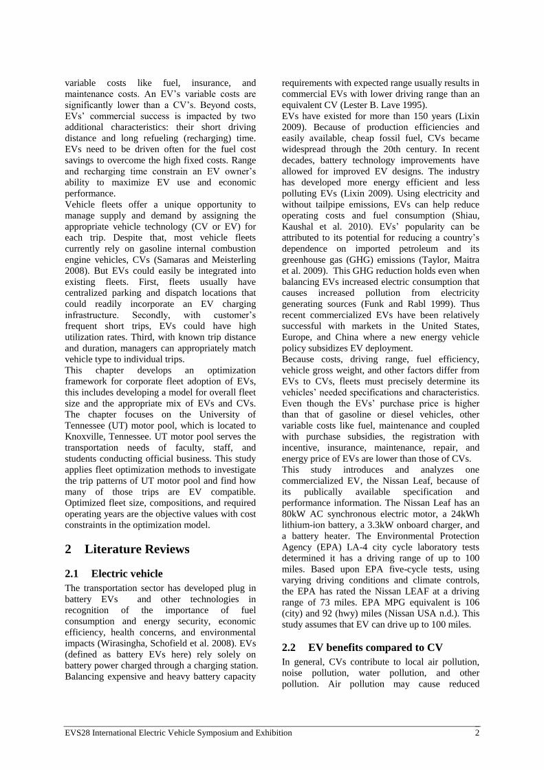
The depreciation rates by vehicle age and model
are shown in Figure 2. Since the Avenger
(launched in 2008) and the Leaf (launched in
2011) do not have a long history, four vehicles--
the Dodge Avenger, the Ford Focus, the Toyota
Prius, and the Nissan Leaf--were compared. The
Ford Focus represents US manufactured vehicles
and the Toyota Prius represents Hybrid vehicles.
As expected, the depreciation rate for a hybrid
vehicle is lower than that of gasoline vehicles
(KBB.com Web 2014). Unlike our expectation,
the Nissan Leaf’s depreciation rate is similar to
the CV’s depreciation rate, perhaps because of
uncertainty with new technology
Figure 2 Depreciation rates by vehicle age and
model
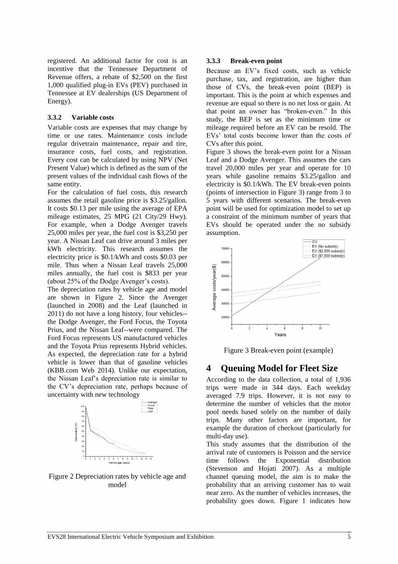
3.3.3 Break-even point
Because an EV’s fixed costs, such as vehicle
purchase, tax, and registration, are higher than
those of CVs, the break-even point (BEP) is
important. This is the point at which expenses and
revenue are equal so there is no net loss or gain. At
that point an owner has “broken-even.” In this
study, the BEP is set as the minimum time or
mileage required before an EV can be resold. The
EVs’ total costs become lower than the costs of
CVs after this point.
Figure 3 shows the break-even point for a Nissan
Leaf and a Dodge Avenger. This assumes the cars
travel 20,000 miles per year and operate for 10
years while gasoline remains $3.25/gallon and
electricity is $0.1/kWh. The EV break-even points
(points of intersection in Figure 3) range from 3 to
5 years with different scenarios. The break-even
point will be used for optimization model to set up
a constraint of the minimum number of years that
EVs should be operated under the no subsidy
assumption.
Figure 3 Break-even point (example)
4 Queuing Model for Fleet Size
According to the data collection, a total of 1,936
trips were made in 344 days. Each weekday
averaged 7.9 trips. However, it is not easy to
determine the number of vehicles that the motor
pool needs based solely on the number of daily
trips. Many other factors are important, for
example the duration of checkout (particularly for
multi-day use).
This study assumes that the distribution of the
arrival rate of customers is Poisson and the service
time follows the Exponential distribution
(Stevenson and Hojati 2007). As a multiple
channel queuing model, the aim is to make the
probability that an arriving customer has to wait
near zero. As the number of vehicles increases, the
probability goes down. Figure 1 indicates how
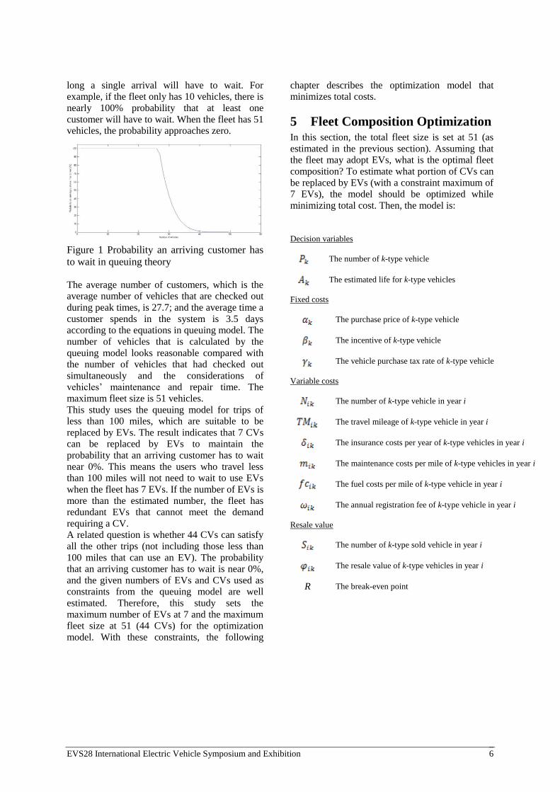
EVS28 International Electric Vehicle Symposium and Exhibition 6
long a single arrival will have to wait. For
example, if the fleet only has 10 vehicles, there is
nearly 100% probability that at least one
customer will have to wait. When the fleet has 51
vehicles, the probability approaches zero.
Figure 1 Probability an arriving customer has
to wait in queuing theory
The average number of customers, which is the
average number of vehicles that are checked out
during peak times, is 27.7; and the average time a
customer spends in the system is 3.5 days
according to the equations in queuing model. The
number of vehicles that is calculated by the
queuing model looks reasonable compared with
the number of vehicles that had checked out
simultaneously and the considerations of
vehicles’ maintenance and repair time. The
maximum fleet size is 51 vehicles.
This study uses the queuing model for trips of
less than 100 miles, which are suitable to be
replaced by EVs. The result indicates that 7 CVs
can be replaced by EVs to maintain the
probability that an arriving customer has to wait
near 0%. This means the users who travel less
than 100 miles will not need to wait to use EVs
when the fleet has 7 EVs. If the number of EVs is
more than the estimated number, the fleet has
redundant EVs that cannot meet the demand
requiring a CV.
A related question is whether 44 CVs can satisfy
all the other trips (not including those less than
100 miles that can use an EV). The probability
that an arriving customer has to wait is near 0%,
and the given numbers of EVs and CVs used as
constraints from the queuing model are well
estimated. Therefore, this study sets the
maximum number of EVs at 7 and the maximum
fleet size at 51 (44 CVs) for the optimization
model. With these constraints, the following
chapter describes the optimization model that
minimizes total costs.
5 Fleet Composition Optimization In this section, the total fleet size is set at 51 (as
estimated in the previous section). Assuming that
the fleet may adopt EVs, what is the optimal fleet
composition? To estimate what portion of CVs can
be replaced by EVs (with a constraint maximum of
7 EVs), the model should be optimized while
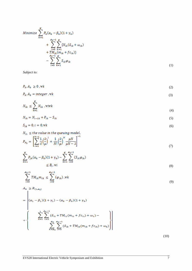
minimizing total cost. Then, the model is:
Decision variables
The number of k-type vehicle
The estimated life for k-type vehicles
Fixed costs
The purchase price of k-type vehicle
The incentive of k-type vehicle
The vehicle purchase tax rate of k-type vehicle
Variable costs
The number of k-type vehicle in year i
The travel mileage of k-type vehicle in year i
The insurance costs per year of k-type vehicles in year i
The maintenance costs per mile of k-type vehicles in year i
The fuel costs per mile of k-type vehicle in year i
The annual registration fee of k-type vehicle in year i
Resale value
The number of k-type sold vehicle in year i
The resale value of k-type vehicles in year i
R The break-even point
EVS28 International Electric Vehicle Symposium and Exhibition 7
(1)
Subject to:
(2)
(3)
(4)
(5)
(6)
(7)
(8)
(9)
(10)

EVS28 International Electric Vehicle Symposium and Exhibition 8
The objective function (1) minimizes the total
costs associated with fixed costs, variable costs,
and resale value with discounted cash flows.
Since the UT motor pool fleet is a self-insured
fleet, this study assumes that the average
insurance rate reflects expected losses. The
constraints (2) and (3) require a non-negative and
integer solution for all decision variables.
The constraints given in (4) through (7) are the
number of vehicles constraints. Constraint (4)
enforces the total number of k-type vehicles in
year i could not exceed the total number of
vehicles in year i. Constraint (5) ensures that the
total number of k-type vehicles in year i should be
equal to the gap between number of purchased
and sold k-type vehicles in year i. Constraint (6)
ensures that the fleet cannot sell a vehicle that is
less than one year old. Constraint (7) assures that
the number of EVs could not exceed the value
attained in the queuing analysis presented above,
which assures full availability of the fleet.
The constraints given in (8) through (9) are costs
constraints. Constraint (8) limits total spending in
i year so it will not exceed the fleet budget.
Constraint (9) enforces that total annual
maintenance costs should not exceed the resale
value. Fuel costs are calculated by using fuel
efficiency such as mile per gallon and mile per
kWh and average fuel price per unit (gallon or
kWh).
Constraint (10) enforces that the minimum
estimated life for k-type vehicles in year i should
be longer than the break-even year, assuring that
the increased capital cost of EVs are recovered in
fuel and maintenance savings before resale.
6 Results The optimization model was built using IBM
ILOG CPLEX Optimization studio 12.5. The
computer is a laptop with an Intel Core i5-3210M
CPU @ 2.50 GHz with 6 GB of RAM memory.
The time spend to generate a solution is 20.04
seconds.
Table 2 Optimization results
Number
of
vehicles
Travel mileage
per year
Years need
to be
operated
Total
costs/vehicle/year
(resale value
included)
EVs 7 10,218 miles 4.5 $ 6,062
Gasoline
Vehicles 44 20,193 miles 3 $ 10,116
The number of vehicles assure near zero expected
waiting delay is 51 from the queuing model. The
optimization results show that all trips less than
100 miles can be replaced by EVs with minimum
total costs and those EVs should be operated for
at least 4.5 years, which is later than the break-
even point. Average annual total mileages
estimated by the model appear reasonable
compared with real data and the sum of total
mileage satisfies the total fleet mileage demands.
The total cost of ownership would be minimized
with the estimated values, which means that the
fleet can be operated with a minimized budget
when 7 EVs and 44 CVs are operated for 4.5 and
3 years, respectively. It shows that even though
EV depreciation rate is lower than CV
depreciation, depreciation costs account for the
biggest portion of EV’s average total costs per
year because of high purchase price and low fuel
and maintenance costs. It also shows the
differences for maintenance and fuel costs. Fuel
and maintenance costs for a CV account for 27%
and 17% respectively. On the other hand, for an
EV they account for only 6% and 2% for EV.
This indicates that fuel price and efficiency are
the most significant factors for a CV while a
subsidy incentive to lower high purchase price is
the most significant factor to promote EV usage.
6.1 Sensitivity analysis
We now examine the sensitivity analysis for
change of years that need to be operated. EVs
need to be operated a minimum range of 5 to 10
years while CVs have a minimum range of 3 to 5
years. That is, EVs and CVs should be operated
for at least 5 and 3 years, respectively. An EV can
be operated up to 10 years and a CV may be used
up to 5 years to satisfy the minimum total costs
condition.
We use 3 different fuel efficiencies for each
vehicle type to investigate how model sensitivities
are affected by fuel efficiency. CVs require 22
miles per gallon (mpg), 25 mpg, and 50 mpg, the
highest fuel efficiency for the Toyota Prius, a
hybrid vehicle. EVs have a higher purchase price
and efficiency ranges (mile per kWh) are 2
mi/kWh, 3 mi/kWh, and 4 mi/kWh. As shown in
Figure 5, the EV requirement years to minimize
total costs increase as CV mpg improves. That is,
EVs become less competitive with the adoption of
improved fuel efficiency CVs like traditional
hybrids. CV required operating duration remains
3 years. Due to increased maintenance costs and
decreased depreciation cost, the fleet would
improve by selling old vehicles and buy new ones
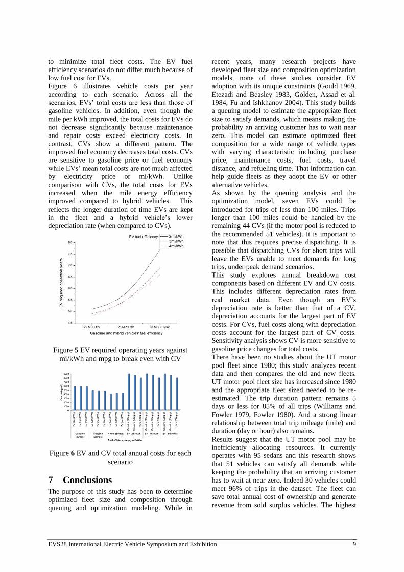
EVS28 International Electric Vehicle Symposium and Exhibition 9
to minimize total fleet costs. The EV fuel
efficiency scenarios do not differ much because of
low fuel cost for EVs.
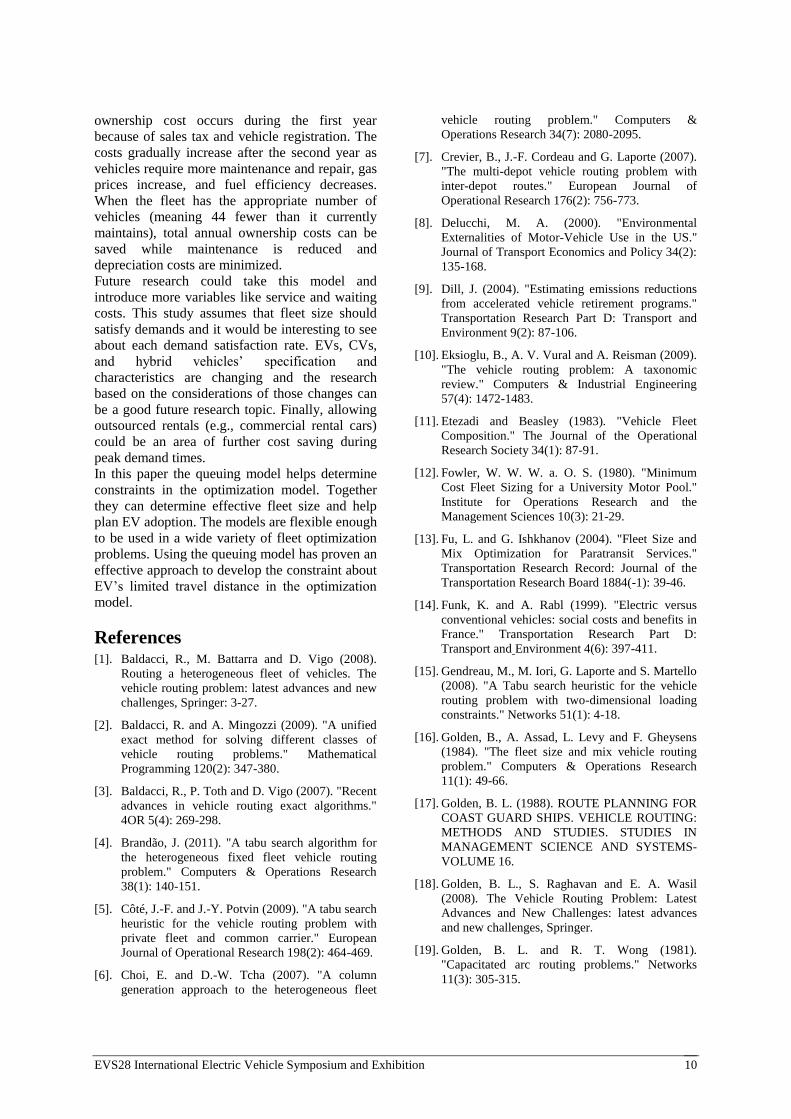
Figure 6 illustrates vehicle costs per year
according to each scenario. Across all the
scenarios, EVs’ total costs are less than those of
gasoline vehicles. In addition, even though the
mile per kWh improved, the total costs for EVs do
not decrease significantly because maintenance
and repair costs exceed electricity costs. In
contrast, CVs show a different pattern. The
improved fuel economy decreases total costs. CVs
are sensitive to gasoline price or fuel economy
while EVs’ mean total costs are not much affected
by electricity price or mi/kWh. Unlike
comparison with CVs, the total costs for EVs
increased when the mile energy efficiency
improved compared to hybrid vehicles. This
reflects the longer duration of time EVs are kept
in the fleet and a hybrid vehicle’s lower
depreciation rate (when compared to CVs).
Figure 5 EV required operating years against
mi/kWh and mpg to break even with CV
Figure 6 EV and CV total annual costs for each
scenario
7 Conclusions
The purpose of this study has been to determine
optimized fleet size and composition through
queuing and optimization modeling. While in
recent years, many research projects have
developed fleet size and composition optimization
models, none of these studies consider EV
adoption with its unique constraints (Gould 1969,
Etezadi and Beasley 1983, Golden, Assad et al.
1984, Fu and Ishkhanov 2004). This study builds
a queuing model to estimate the appropriate fleet
size to satisfy demands, which means making the
probability an arriving customer has to wait near
zero. This model can estimate optimized fleet
composition for a wide range of vehicle types
with varying characteristic including purchase
price, maintenance costs, fuel costs, travel
distance, and refueling time. That information can
help guide fleets as they adopt the EV or other
alternative vehicles.
As shown by the queuing analysis and the
optimization model, seven EVs could be
introduced for trips of less than 100 miles. Trips
longer than 100 miles could be handled by the
remaining 44 CVs (if the motor pool is reduced to
the recommended 51 vehicles). It is important to
note that this requires precise dispatching. It is
possible that dispatching CVs for short trips will
leave the EVs unable to meet demands for long
trips, under peak demand scenarios.
This study explores annual breakdown cost
components based on different EV and CV costs.
This includes different depreciation rates from
real market data. Even though an EV’s
depreciation rate is better than that of a CV,
depreciation accounts for the largest part of EV
costs. For CVs, fuel costs along with depreciation
costs account for the largest part of CV costs.
Sensitivity analysis shows CV is more sensitive to
gasoline price changes for total costs.
There have been no studies about the UT motor
pool fleet since 1980; this study analyzes recent
data and then compares the old and new fleets.
UT motor pool fleet size has increased since 1980
and the appropriate fleet sized needed to be re-
estimated. The trip duration pattern remains 5
days or less for 85% of all trips (Williams and
Fowler 1979, Fowler 1980). And a strong linear
relationship between total trip mileage (mile) and
duration (day or hour) also remains.
Results suggest that the UT motor pool may be
inefficiently allocating resources. It currently
operates with 95 sedans and this research shows
that 51 vehicles can satisfy all demands while
keeping the probability that an arriving customer
has to wait at near zero. Indeed 30 vehicles could
meet 96% of trips in the dataset. The fleet can
save total annual cost of ownership and generate
revenue from sold surplus vehicles. The highest
EVS28 International Electric Vehicle Symposium and Exhibition 10
ownership cost occurs during the first year
because of sales tax and vehicle registration. The
costs gradually increase after the second year as
vehicles require more maintenance and repair, gas
prices increase, and fuel efficiency decreases.
When the fleet has the appropriate number of
vehicles (meaning 44 fewer than it currently
maintains), total annual ownership costs can be
saved while maintenance is reduced and
depreciation costs are minimized.
Future research could take this model and
introduce more variables like service and waiting
costs. This study assumes that fleet size should
satisfy demands and it would be interesting to see
about each demand satisfaction rate. EVs, CVs,
and hybrid vehicles’ specification and
characteristics are changing and the research
based on the considerations of those changes can
be a good future research topic. Finally, allowing
outsourced rentals (e.g., commercial rental cars)
could be an area of further cost saving during
peak demand times.
In this paper the queuing model helps determine
constraints in the optimization model. Together
they can determine effective fleet size and help
plan EV adoption. The models are flexible enough
to be used in a wide variety of fleet optimization
problems. Using the queuing model has proven an
effective approach to develop the constraint about
EV’s limited travel distance in the optimization
model.
References [1]. Baldacci, R., M. Battarra and D. Vigo (2008).
Routing a heterogeneous fleet of vehicles. The
vehicle routing problem: latest advances and new
challenges, Springer: 3-27.
[2]. Baldacci, R. and A. Mingozzi (2009). "A unified
exact method for solving different classes of
vehicle routing problems." Mathematical
Programming 120(2): 347-380.
[3]. Baldacci, R., P. Toth and D. Vigo (2007). "Recent
advances in vehicle routing exact algorithms."
4OR 5(4): 269-298.
[4]. Brandão, J. (2011). "A tabu search algorithm for
the heterogeneous fixed fleet vehicle routing
problem." Computers & Operations Research
38(1): 140-151.
[5]. Côté, J.-F. and J.-Y. Potvin (2009). "A tabu search
heuristic for the vehicle routing problem with
private fleet and common carrier." European
Journal of Operational Research 198(2): 464-469.
[6]. Choi, E. and D.-W. Tcha (2007). "A column
generation approach to the heterogeneous fleet
vehicle routing problem." Computers &
Operations Research 34(7): 2080-2095.
[7]. Crevier, B., J.-F. Cordeau and G. Laporte (2007).
"The multi-depot vehicle routing problem with
inter-depot routes." European Journal of
Operational Research 176(2): 756-773.
[8]. Delucchi, M. A. (2000). "Environmental
Externalities of Motor-Vehicle Use in the US."
Journal of Transport Economics and Policy 34(2):
135-168.
[9]. Dill, J. (2004). "Estimating emissions reductions
from accelerated vehicle retirement programs."
Transportation Research Part D: Transport and
Environment 9(2): 87-106.
[10]. Eksioglu, B., A. V. Vural and A. Reisman (2009).
"The vehicle routing problem: A taxonomic
review." Computers & Industrial Engineering
57(4): 1472-1483.
[11]. Etezadi and Beasley (1983). "Vehicle Fleet
Composition." The Journal of the Operational
Research Society 34(1): 87-91.
[12]. Fowler, W. W. W. a. O. S. (1980). "Minimum
Cost Fleet Sizing for a University Motor Pool."
Institute for Operations Research and the
Management Sciences 10(3): 21-29.
[13]. Fu, L. and G. Ishkhanov (2004). "Fleet Size and
Mix Optimization for Paratransit Services."
Transportation Research Record: Journal of the
Transportation Research Board 1884(-1): 39-46.
[14]. Funk, K. and A. Rabl (1999). "Electric versus
conventional vehicles: social costs and benefits in
France." Transportation Research Part D:
Transport and Environment 4(6): 397-411.
[15]. Gendreau, M., M. Iori, G. Laporte and S. Martello
(2008). "A Tabu search heuristic for the vehicle
routing problem with two-dimensional loading
constraints." Networks 51(1): 4-18.
[16]. Golden, B., A. Assad, L. Levy and F. Gheysens
(1984). "The fleet size and mix vehicle routing
problem." Computers & Operations Research
11(1): 49-66.
[17]. Golden, B. L. (1988). ROUTE PLANNING FOR
COAST GUARD SHIPS. VEHICLE ROUTING:
METHODS AND STUDIES. STUDIES IN
MANAGEMENT SCIENCE AND SYSTEMS-
VOLUME 16.
[18]. Golden, B. L., S. Raghavan and E. A. Wasil
(2008). The Vehicle Routing Problem: Latest
Advances and New Challenges: latest advances
and new challenges, Springer.
[19]. Golden, B. L. and R. T. Wong (1981).
"Capacitated arc routing problems." Networks
11(3): 305-315.

EVS28 International Electric Vehicle Symposium and Exhibition 11
[20]. Gould, J. (1969). "The Size and Composition of a
Road Transport Fleet." OR 20(1): 81-92.
[21]. Hadley, S. W. and A. A. Tsvetkova (2009).
"Potential Impacts of Plug-in Hybrid Electric
Vehicles on Regional Power Generation." The
Electricity Journal 22(10): 56-68.
[22]. KBB.com Web. (2014). "Used car resale value."
Retrieved 3-13, 2014, from kbb.com.
[23]. Kim, H. C., G. A. Keoleian, D. E. Grande and J. C.
Bean (2003). "Life Cycle Optimization of
Automobile Replacement: Model and
Application." Environmental Science &
Technology 37(23): 5407-5413.
[24]. Laporte, G. (2009). "Fifty Years of Vehicle
Routing." Transportation Science 43(4): 408-416.
[25]. Lester B. Lave, C. T. H., Francis Clay Mcmichael
(1995). Environmental implications of electric
cars. Sience, Research Library Core. 268: 993.
[26]. Lixin, S. (2009). Electric Vehicle development:
The past, present & future. Power Electronics
Systems and Applications, 2009. PESA 2009. 3rd
International Conference on.
[27]. Loxton, R., Q. Lin and K. L. Teo (2012). "A
stochastic fleet composition problem." Computers
& Operations Research 39(12): 3177-3184.
[28]. Nissan USA. (n.d.). "Nissan USA." Retrieved
Mar 14, 2014, from http://www.nissanusa.com/.
[29]. Parrish, D. D. (2006). "Critical evaluation of US
on-road vehicle emission inventories."
Atmospheric Environment 40(13): 2288-2300.
[30]. Penna, P. H. V., A. Subramanian and L. S. Ochi
(2013). "An iterated local search heuristic for the
heterogeneous fleet vehicle routing problem."
Journal of Heuristics 19(2): 201-232.
[31]. Prins, C. (2009). A GRASP× evolutionary local
search hybrid for the vehicle routing problem.
Bio-inspired algorithms for the vehicle routing
problem, Springer: 35-53.
[32]. Rexeis, M. and S. Hausberger (2009). "Trend of
vehicle emission levels until 2020 – Prognosis
based on current vehicle measurements and future
emission legislation." Atmospheric Environment
43(31): 4689-4698.
[33]. Samaras, C. and K. Meisterling (2008). "Life
Cycle Assessment of Greenhouse Gas Emissions
from Plug-in Hybrid Vehicles: Implications for
Policy." Environmental Science & Technology
42(9): 3170-3176.
[34]. Shiau, C.-S. N., N. Kaushal, C. T. Hendrickson, S.
B. Peterson, J. F. Whitacre and J. J. Michalek
(2010). "Optimal Plug-In Hybrid Electric Vehicle
Design and Allocation for Minimum Life Cycle
Cost, Petroleum Consumption, and Greenhouse
Gas Emissions." Journal of Mechanical Design
132(9): 091013-091011.
[35]. Simms, B. W., B. G. Lamarre, A. K. S. Jardine
and A. Boudreau (1984). "Optimal buy, operate
and sell policies for fleets of vehicles." European
Journal of Operational Research 15(2): 183-195.
[36]. Sims, R. E. H., H.-H. Rogner and K. Gregory
(2003). "Carbon emission and mitigation cost
comparisons between fossil fuel, nuclear and
renewable energy resources for electricity
generation." Energy Policy 31(13): 1315-1326.
[37]. Stevenson, W. J. and M. Hojati (2007).
Operations management, McGraw-Hill/Irwin
Boston.
[38]. Taylor, J., A. Maitra, M. Alexander, D. Brooks
and M. Duvall (2009). Evaluation of the impact of
plug-in electric vehicle loading on distribution
system operations. Power & Energy Society
General Meeting, 2009. PES '09. IEEE.
[39]. Thibaut Vidal, T. G. C., Michel Gendreay,
Christian Prins (2012). Heuristics for Multi-
Attribute Vehicle Routing Problems: A Survey
and Synthesis, Interuniversity Research Centre of
Enterprise Networks, Logistics and Transportation.
CIRRELT-2012-05.
[40]. Toth, P. and D. Vigo (2001). The vehicle routing
problem, Siam.
[41]. US Department of Energy. "US Department of
Energy." Retrieved March 14, 2013, from
http://www.energy.gov/.
[42]. Williams, W. W. and O. S. Fowler (1979).
"MODEL FORMULATION FOR FLEET SIZE
ANALYSIS OF A UNIVERSITY MOTOR
POOL." Decision Sciences 10(3): 434-450.
[43]. Wirasingha, S. G., N. Schofield and A. Emadi
(2008). Plug-in hybrid electric vehicle
developments in the US: Trends, barriers, and
economic feasibility. Vehicle Power and
Propulsion Conference, 2008. VPPC '08. IEEE.
Authors
Taekwan Yoon is a business
development specialist at LG CNS.
Dr. Yoon got Master’s (2008) and
Ph.D. (2014) degrees from Seoul
National University in Republic of
Korea and the University of
Tennessee, Knoxville, respectively.
Dr. Yoon’s research areas are
sustainable transportation (electric
vehicle, carsharing, bike sharing),
ITS, pedestrian behavior and
vehicle fleet optimization.

EVS28 International Electric Vehicle Symposium and Exhibition 12
Chris R. Cherry is an associate
professor at the University of
Tennessee, Knoxville. Dr. Cherry
got a Master’s and Ph.D. degrees
from University of Arizona and
University of California, Berkeley,
respectively. Dr. Cherry is
interested in transportation
planning, economics, and
sustainability.
Related Documents