E uropean J ournal of G eography Volume 6 • Number 4 • December 2015 • ISSN 1792-1341 European Association of Geographers

Welcome message from author
This document is posted to help you gain knowledge. Please leave a comment to let me know what you think about it! Share it to your friends and learn new things together.
Transcript
European Journal of Geography
Volume 6 • Number 4 • December 2015 • ISSN 1792-1341
E u r o p e a n A s s o c i a t i o n o f G e o g r a p h e r s
1
European Journal of Geography The publication of the EJG (European Journal of Geography) is based on the European Association of Geographers’ goal to make European higher education a worldwide reference and standard. Thus, the scope of the EJG is to publish original and innovative papers that will substantially improve, in a theoretical, conceptual or empirical way the quality of research, learning, teaching and applying geography, as well as in promoting the significance of geography as a discipline. Submissions should have a European dimension. Contributions to EJG are welcomed. They should conform to the Notes for authors and should be submitted to the Editor, as should books for review. The content of this journal does not necessarily represent the views or policies of EUROGEO except where explicitly identified as such. Editor
Kostis C. Koutsopoulos Professor, National Technical University of Athens, Greece [email protected]
Associate Editor Yorgos N. Photis Associate Professor, National Technical University of Athens, Greece [email protected]
Editorial Advisory Board
Ari Yilmaz, Prof., Balikesir University, Turkey Bailly Antoine, Prof., University of Geneva, Geneva Switzerland Bellezza Giuliano, Prof., University of Tuscia, Viterbo, Italy Buttimer Anne, Prof., University College Dublin, Ireland Chalkley Brian, Prof., University of Plymouth, Plymouth UK Gesar Anton, Prof., University of Primorska, Slovenia Haubrich Hartwig, Prof., University of Education, Freiburg, Germany Martin Fran, S. Lecturer, University of Exeter, UK Strobl Josef, Prof., University of Salzburg, Salzburg, Austria Van der Schee Joop, Prof., VU University, The Nederlands
© EUROGEO, 2015 ISSN 1792-1341
The European Journal of Geography is published by EUROGEO - the European Association of Geographers (www.eurogeography.eu).
2
European Journal of Geography
Volume 6, Number 4 December 2015
C O N T E N T S
4 Letter from the Editor
6 DO PERSONAL EXPERIENCES HAVE AN IMPACT ON TEACHING AND DIDACTIC CHOICES IN GEOGRAPHY? Lena MOLIN, Ann GRUBBSTROM, Gabriel BLADH, Asa WESTERMARK, Kaj OJANNE, Hans-Olof GOTTFRIDSSON and Svante KARLSSON
21 TREES OUTSIDE FOREST IN THE AGRARIAN LANDSCAPE OF MEDITERRANEAN MOUNTAIN REGIONS: THE CASE OF SIERRA DE LA CONTRAVIESA, SPAIN. Jesus CAMACHO CASTILLO, Laura PORCEL RODRIGUEZ, Yolanda JIMENEZ OLIVENCIA and Antonia PANIZA CABRERA
35 ASSESSING SUSTAINABILITY IN COASTAL TOURISM SECTORS OF ODISHA COAST, INDIA. Nilay Kanti BARMAN, Goutam BERA and Mihir Kumar PRADHAN
51 IDENTIFICATION OF WEAKNESSES AND STRENGTHS OF TOURISM
DEVELOPMENT IN KANDOLEH VILLAGE, IRAN.
Aeizh AZMI and Akram RAZLANSARI
59
SCENARIO-BASED LOCATION OF AMBULANCES FOR SPATIOTEMPORAL CLUSTERS OF EVENTS AND STOCHASTIC VEHICLE AVAILABILITY. A DECISION SUPPORT SYSTEMS APPROACH. Yorgos N. PHOTIS and Stavros A. SIRIGOS
76 FALLING DOMINOS OR THE ROLE OF GEOGRAPHIC MENTAL MAPS IN FOREIGN POLICY. Luis M. DA VINHA
88 MORPHOMETRIC ANALYSIS OF HYDROLOGICAL BEHAVIOR OF NORTH FARS WATERSHED, IRAN.
Marzieh MOKARRAM and Dinesh SATHYAMOORTHY

3
4
Editorial
The publication of the European Journal of Geography (EJG) is based on the European Association of Geographers’ goal to make European Geography a worldwide reference and standard. As a result, the papers published in the EJG, including those on this issue, are focused in promoting the significance of geography as a discipline, in resolving global issues or applying geography, complementing, of course, the fundamental goals of improving the quality of research, learning and teaching of Geography. In other words with the EJG the European Association of Geographers provides a forum for geographers worldwide to communicate on all aspects of research and applications of geography with a European dimension, but not exclusive. As a result, every issue of the EJG provides a glimpse of the important role Geography can play in helping researchers, academics, professionals as well as decision makers and politicians in resolving a wide spectrum of problems. In other words, EJG following Geography which connects the physical, human and technological sciences is aiming at enhancing teaching, research, and of interest to decision makers, problem solving. That is, in every issue of the journal a reader can find answers of how aspects of these sciences are interconnected and are forming spatial patterns and processes that impact on global issues and thus effecting present and future generations. The goal of the editorial team, which up to now has been achieved to a great extent, is that the papers of the EJG by dealing with places, people and cultures, will explore those issues ranging from physical, urban and rural environments and their evolution to climate, pollution, development and political-economy. Thus, your contributions to the EJG are not only desirable, but necessary for Geography and Science as a whole. Kostis C. Koutsopoulos
Editor EJG

5
European Journal of Geography, 6:4 Copyright © European Association of Geographers, 2015 ISSN 1792-134
European Journal of Geography Volume 6, Number 4:6 - 20, December 2015
©Association of European Geographers
European Journal of Geography-ISSN 1792-1341 © All rights reserved 6
DO PERSONAL EXPERIENCES HAVE AN IMPACT ON TEACHING AND
DIDACTIC CHOICES IN GEOGRAPHY?
Lena MOLIN Uppsala University, Department of Education, Sweden
www.edu.uu.se
Ann GRUBBSTRÖM Uppsala University, Department of Social and Economic Geography
www.kultgeog.uu.se
Gabriel BLADH
Karlstad University,Department of Geography, Media and Communication
www.kau.se [email protected]
Åsa WESTERMARK Jönköping University, School of Education and Communication
www.ju.se
Kaj OJANNE
Lund University, The Department of Human Geography and the Human Ecology Division
www.keg.lu.se [email protected]
Hans-Olof GOTTFRIDSSON Karlstad University, Department of Geography, Media and Communication
Svante KARLSSON Umeå University, Department of Geography and Economic History
www.geoekhist.umu.se
Abstract
Factors influencing teachers’ selection of content in geography teaching is a fundamental
didactic matter. 1 The purpose of the present study was to investigate whether Swedish
geography teachers’ informal and formal experiences have influenced their interest in
geography and if so, in what way. The results disclosed that informal experiences like
outings, holidays, and childhood memories have a significant impact. The results also
revealed that childhood experiences might increase the comprehension of how nature and
1 In this article we use the terms didactics and subject matter didactics, being well aware that the common use of
didactics in English is different from the use of didaktik in the Scandinavian languages. However, we are here
connecting to the Nordic and continental philosophical traditions of didactics.

Molin L., et al. / European Journal of Geography 6 4 6–20 (2015)
European Journal of Geography-ISSN 1792-1341 © All rights reserved 7
mankind are connected, and how various places differ. Selective traditions showed to be
strong, i.e. geographic names and map reading were prioritized while at excursions, physical
geography was particularly dominating. We argue that in the geography teacher education,
didactics should include methods for field studies, giving emphasis also to the part dealing
with human geography. Forthcoming teachers need to reflect on how to make didactic choices
in order to renounce the selective traditions in the subject.
Keywords: geography teachers, informal and formal experiences, reflection, selective traditions,
subject skills
1. INTRODUCTION
Factors affecting how geography teachers perform their education are of great didactic
significance. More knowledge about these might improve our capability to link teacher
education to student teachers’ own experiences. This will motivate and engage the student
teachers in their own subject studies as well as in their own teaching. It will furthermore
create more knowledge about which factors that affect educators’ teaching, and increase their
awareness about their own didactic choices, i.e. what purpose, content, and method they
decide on for each new lesson, didactic choices of uttermost importance to the pupils’
learning. Acquiring the ability to reflect on one’s own didactic choices involves systematic
practicing.
John Dewey (1933) concluded that all education needs to contain reflective thinking, and
defined the concept of reflection as “an active, persistent, and careful consideration of any
belief or supposed form of knowledge in light of the grounds supporting it and future
conclusions to which it tends” (p. 6). Dewey’s thoughts about the importance of developing
reflection capability in an education context procured several followers, e.g. Schön (1983,
1987), who argued that a teacher can improve his/her teaching by constantly reflecting on
his/her teaching practice, and through this develop different degrees of comprehension of
his/her own role as an educator.
Other scientists considering reflection as one of the most important activities in teacher
education and teaching are Zeichner and Liston (1996), Rodgers (2002), Griffin (2003), Lee
(2005), Geerinck, Masschelein and Simons (2010), Henry and Bruland (2020), and Mackay
and Tymon (2013). Reflecting is conceived as an intellectual process oriented toward an
object or a profession, and aims at acquiring a deeper understanding of the profession or of
one’s self, the purpose being to reflect one’s profession in one’s self. To achieve this, teachers
and student teachers need education in didactics, where concept, theories, and knowledge of
the subject are combined to construct an active reflection process in linkage with investigating
one’s own practice (Ongstad, 2006; Schüllerqvist, 2009). We anticipate that the results
acquired in the present study will be useful for teacher educators and student teachers as part
of this reflection process. Teachers’ subject comprehension is a vital starting point for their
choice of profession and their didactic choices in teaching.
Our study was inspired by an article by Catling, Greenwood, Martin and Owens (2010),
who reported on a study investigating whether previous experiences in life had affected their
interest in studying geography and working as a geography teacher in primary school in Great
Britain and Ireland, and if so, in what manner. Research in and about the school subject
geography is limited in Sweden, and to our knowledge no studies exist on which factors that
have influenced geography teachers to choose this subject. There are, however, studies
investigating student teachers’ and secondary school teachers’ selection of content (Molin,
2006) and teachers’ views on geography at the upper (Wennberg, 1990) and intermediate
levels of elementary school (Molin & Grubbström, 2013). Studies have furthermore reported
Molin L., et al. / European Journal of Geography 6 4 6–20 (2015)
European Journal of Geography-ISSN 1792-1341 © All rights reserved 8
on teachers’ as well as student teachers’ views on the subject (Ojanne, 1990; Nilsson, 2009;
Gottfridsson & Bladh, 2012; Bladh, 2014). The present study thus supplements previous
research in that it focused on Swedish geography teachers and disclosed which experiences in
early life that had an impact on their choice of profession. A further purpose was to
investigate the factors that influence the teachers’ didactic choices, i.e. the purpose of their
teaching, the content they select, and which methods they use, along with their opinions about
the new syllabuses and national tests.
2. THE SWEDISH CONTEXT
One plausible reason for the lack of research in and about geography as a school subject
might be the weak position the subject presently holds in school. The reason behind this weak
position in Sweden is an interesting question, as this was not always the case. On the contrary,
looking back at the 16th century, geography was a high status subject within the seven free
arts. Carl von Linné furthered the subject by his field studies and observations, and geography
was an important school subject during the 18th century (Buttimer & Mels, 2006). From the
middle of the 19th century, geography was studied in coalition with history, but became an
independent subject in the first five school years in 1895, and from 1909 also in secondary
school (Olsson, 1986). Geography was promoted as a subject in the building of the Swedish
nation, and the early 20th century was a formative period for geography, in school as well as
academically. A strong tradition of regional geography was established during this period.
The interest in geopolitics during the initial time of the first and second world wars, from
which Sweden by its neutrality was spared, also brought about an increased interest in
geography, map reading, and issues of the outside world. During the 1960’s, however,
something happened that affected the school subject geography negatively, and a stagnation
of the contents can be derived from this point in time. Geography as a science was divided
into human geography and physical geography at the Swedish universities, which led to the
subject being split into different institutes and faculties (social sciences and natural sciences).
Hence, the interest in the coherent school subject geography diminished, and the desire to
obtain a teacher education in geography decreased. The academic split furthermore had
consequences for the subject in secondary school, from where it disappeared in 1965.
Geography knowledge was instead incorporated into the new subjects civics and science. In
1994, geography was reintroduced as a subject, but has continued to have a weak position in
secondary school, which has affected its status as a school subject (Bladh & Molin, 2012).
2.1. Subject integration or subject specialization
Geography belongs in Sweden to the social science subjects (geography, history, religion,
civics), similarly to e.g. Norway, England, and the USA, as in contrast to other countries, e.g.
Finland and Denmark, where geography is a subject within natural sciences (Bladh & Molin,
2012). Whether some school subjects should be organized as Social studies (socially oriented;
geography, history, religion, civics) or exist as separate subjects, has been under discussion –
occasionally very lively – since the 1960’s, and the discussion is still ongoing (Samuelsson,
2014). How to organize subjects is linked to what knowledge the teaching should convey and
how grades are set, i.e. four grades in the separate subjects or one block grade in Social
studies.
At two occasions between the beginning of the 20th century and to date, the separate
subjects were fused into one SO-subject with a common syllabus and common criteria for
grading. It started in the beginning of the 1960’s when Sweden commenced a nine-year
compulsory elementary school with a new curriculum (Lgr 62), in which orientating subjects
Molin L., et al. / European Journal of Geography 6 4 6–20 (2015)
European Journal of Geography-ISSN 1792-1341 © All rights reserved 9
were introduced as one concept that was divided into Science Studies (NO) and Social studies
(SO). Next curricular reform (Lgr 69) maintained the orientating subjects, one overarching
purpose being to convey to the pupil “knowledge about the surrounding reality and about
people’s lives and activities in the past and at present”. The curricular reform Lgr 80 still
emphasized that teaching should be subject overarching. The subject labels were abolished
and replaced by a number of themes in Social studies, e.g. Surroundings of Mankind and
Activities of Mankind – the time perspective.
In the beginning of the 20th century, comprehensive educational reforms were
implemented, changing the state school into a municipally governed school, and introducing
private schools, enabling private ownership of schools. New steering principles were
instituted: goal and result guidelines, entailing e.g. new syllabuses and a new grading system
(Lpo 94). In the elementary school, the subject labels for the SO-block were reintroduced,
while the joint comprehensive purpose of Social studies disappeared. A few years later, in the
year 2000, it was once more time to revise the syllabuses, the reason being that the clarity of
the syllabuses needed to be improved. This was achieved by introducing new grading criteria
along with a coherent SO-syllabus. However, the subject plans of 1994 were kept intact. The
teachers decided themselves whether to conduct subject-separated teaching or a subject-
integrated SO-teaching, following the new SO-syllabus.
In 2011, a larger curricular reform (Lgr 11 and Lgy 11) was implemented, introducing new
syllabuses and a new grading system. Social studies was kept intact for years 1-3, but for
years 4-6 and 7-9, new syllabuses for the separate subjects were formulated. This latest
curricular reform is even stronger emphasizing perspectives where understanding geographic
contexts and relations – such as resource conflicts and vulnerability – is covered, and where a
value-based geography with themes like environmental and sustainable development are
highlighted.
Even though the school subject geography has been reorganized several times during the
last fifty years, the academic break-up of the subject into human and physical geography has
remained, which has resulted in student teachers at many universities and university colleges
studying geography as two separate subjects, which in turn makes it problematic for them to
convey the content of the joint geography subject. The teaching in school is consequently
conducted much the same as at the universities, i.e. a separation of human and physical
geography (Molin, 2006). Another problem is that subject didactics to a large extent are
missing in the education of student teachers. At several institutes educating subject teachers in
Sweden, schoolteachers with no education in didactics (not just geography) have since long
been the ones responsible for teaching subject didactics.2
2.2. Subject status
Being a subject within Social studies, geography became synonymous with geographic names
and blind maps, and this concept persists. Geography is today a subject that in elementary
school as well as secondary school has a large number of uneducated teachers. Along with
Swedish as second language, technology, art, Spanish, music, domestic science and consumer
knowledge, geography is on the schools’ top ten-lists of subjects with the highest proportion
of uneducated teachers. According to a report by the National Agency for Education
geography is a subject with less than fifty percent of the teachers being eligible. Gottfridsson
and Bladh reported on one third of the teachers completely lacking education in geography,
2 This situation changed with the teacher education reform 2010, when all subject institutes educating teacher
students were obliged to verify that subject didactics were responsible for the teaching in didactics of the subject
in question. If the subject institute had no subject didactic, its examination right was withdrawn.
Molin L., et al. / European Journal of Geography 6 4 6–20 (2015)
European Journal of Geography-ISSN 1792-1341 © All rights reserved 10
while just above one quarter had an education corresponding to the eligibility of a newly
examined teacher (Bladh, 2014). A large group of eligible teachers at the upper level of
elementary school of today had attained one semester of studies in combination with teaching
experience.
The presently prevailing curricular reform (Lgr 11 and Lgy 11) was inaugurated in 2011,
and resulted in the geography subject losing its status in secondary school, no longer being
included in the common program subjects (subjects that all pupils study regardless of program
choice) such as history, religion, and civics.
A decision to initiate national tests in the separate SO-subjects for years 6 and 9, starting in
spring semester 2013, recently raised the status of geography in elementary school.
Regretfully, the decision was revoked at the government shift, and in spring semester 2015,
national tests in the separate SO-subjects were abolished for year 6.
The large proportion of geography teachers being uneducated has resulted in a
conservation of the subject’s teaching traditions. Previous studies have revealed strong
selective traditions in secondary school’s geography teaching (Molin, 2006; Ojanne, 1999;
Holmén & Anderberg, 1993; Wennberg, 1990). In the years 4-6, i.e. the intermediate level of
elementary school, the selective traditions primarily entail geographic names with the
following working process: the provinces of Sweden, Sweden, the Nordic countries, and
Europe. The world outside Europe is included in the education only at the upper level of
elementary school (Molin & Grubbström, 2013).
Bladh (2014) reports that at the intermediate level, teachers use climate, habitat types, and
geographic names as the most important themes in their teaching, and “…a regional
geographic tradition with knowledge about countries and numerous geographic names are still
prominent” (p. 164). There are indications of core value perspectives, linked with issues about
sustainable development, environment and justice, being dealt with to a higher degree in the
geography teaching of the upper level of elementary school. Geography is however mostly
presented in the form of thematic advances in specialized human or physical geography, with
a relatively weakly developed holistic perspective. “In conclusion, geography at the
intermediate and upper levels of elementary school emerges to a degree as two different
subjects” (ibid; p. 164).
3. THEORY - SELECTIVE TRADITIONS
In reality, curricular reforms and new steering documents have not resulted in any great
changes in how geography teaching is carried out; it is rather syllabuses from previous
curricula along with the contents of textbooks that govern the educational activities. Studies in
Portugal (Alexandre, 2009) and Slovenia (Kolenc Kolnik, 2010) disclosed that educational
reforms were of minor importance to teachers’ geography teaching; once their university
studies were accomplished, teachers rarely furthered their education in order to reach new
theoretic knowledge about the subject.
Wennberg (1990) showed that in Sweden, the curriculum was a document not very
familiar to geography teachers, and was rarely used in the planning of their teaching.
According to Holmén and Anderberg (1993), the low level of ambition characterizing
geography teaching in elementary school has consequences throughout the whole school
system, i.e. teachers’ low educational level, a lowered subject status, as well as conservation
of pupils’ geographical knowledge and of how the subject is appraised. Similar results were
obtained in a study on secondary school teachers’ purpose and selection of content in
geography (Molin, 2006). In this study, Molin highlighted that traditions in the geography
subject had over time developed into being selective, which means that they included as well
as excluded subject matters, and in conjunction had formed one dominating discourse of the
Molin L., et al. / European Journal of Geography 6 4 6–20 (2015)
European Journal of Geography-ISSN 1792-1341 © All rights reserved 11
school subject. Molin and Grubbström (2013) disclosed that at the intermediate level in
elementary school, geography teaching is steered by selective traditions focusing on
knowledge about individual countries and geographic names.
This static situation might be explained by specific opinions about e.g. purpose, content,
and method, developing over time, and which may be perceived as ideologically cemented
rules of educators’ teaching. These so called selective traditions signify that subject content
and teaching method are taken for granted. Williams (1973) used the concept selective
traditions. Subject traditions emerge from history and reflect specific perceptions associated
with various purposes, content, and methods. As Williams pointed out, selectivity of content
is the main issue: ”…the way in which, from a whole possible area of past and present, certain
meanings and practices are chosen for emphasis, certain other meanings and practices are
neglected and excluded” (ibid; p. 3). Cherryholmes (1988) maintained that competition
between the discourses makes it possible to problematize both education theory and practical
content. Several didactic typologies are often involved, as shown for North America by
Roberts (1988), and by Östman (1995) for science education in Sweden.
The concept selective traditions was introduced in the Swedish research on curriculum
theory by Englund (1986), and was later used by Östman (1995) who suggested that subject
discourses are governed by selective traditions, and that a school subject discourse may
encompass several different selective traditions. The discourses are distinguished by different
values and viewpoints, e.g. different ideologies, knowledge aspects, and by fundamentally
different views of human life competing with each another. Cherryholmes (1998) argued that
this competition is what makes it possible to problematize the education’s theoretical as well
as practical contents.
Educational philosophies form an important foundation for the categorization, and were
utilized also by Molin (2006) in her study on geography teachers in secondary school and
their understanding of purpose, content, and method. This study showed that contemporary
geography teachers’ selection of content are characterized by an essentialist philosophy of
education, which is problematic from a core value perspective, as the curriculum specifically
accentuates these issues to be the responsibility of school and its teaching. If the moral
dimension is missing in geography teaching, the opportunity to discuss issues concerning
solidarity, social justice, equality, ethnicity, and the development of a sustainable society, will
to a great deal be lost (Molin, 2006).
One dominating discourse of the school subject (see above), not being exposed to
competing alternatives, might in the end be perceived as objective, and may consequently not
be questioned. The result may be concretized with the aid of five didactic typologies in the
school subject geography: traditionally value-based, natural science-based, social science-
based, multidisciplinary-based, and actuality- and value-based teaching (Molin, 2006). The
typologies, as they involve separate purposes, contents, and methods, result in teaching
leading to different kinds of meaning creation. The present study revealed that these were
linked to early experiences in life, and that these experiences had affected the teachers’ choice
of profession, their didactic choices, and also their views on new syllabuses and national tests.
The concept selective traditions thus points at teachers’ comprehension and perception of a
subject often being notably resistant and excluding. This made for an interesting issue to
investigate: Are geography teachers’ own experiences in childhood and as adults linked to
their choices of profession and to their comprehension of the subject. With a starting point in
McPartland, Butt and Biddulph (2001), Catling et al. (2010) discussed experiences tied to
learning and geography, and how different forms of memories may be related to such learning
situations. Semantic memories are recognized as information that is received and conveyed as
a result of general experiences, while episodic memories are tied to specific events and
experiences, often associated with active participation and sometimes strong and emotional

Molin L., et al. / European Journal of Geography 6 4 6–20 (2015)
European Journal of Geography-ISSN 1792-1341 © All rights reserved 12
situations. Such specific events and learning situations, which may be considered formative to
the individual, may be linked to informal situations as well as to formal educational contexts.
With the perspective of biographies and lifetime stories (cf. Buttimer, 1983 and Goodson,
1988) in mind, the present study took an interest in identifying which episodic memories with
association to the subject geography that had earned a formative position in the teachers’
interests and choices. Relating this to the subject traditions of geography was also deemed
significant in the light of the obvious selective traditions of the subject.
4. METHOD
Seven researcher and teacher educators in geography education at five different universities
and university colleges in Sweden interviewed operational teachers in elementary and
secondary school with a common interview guide. Each interview started with an open
question where the interviewed teacher explained why he/she had acquired an interest in the
geography subject. We subsequently focused on various themes that related to memories in
their childhood and their educational process from elementary school to university and
university college studies. Finally, the interview pertained to issues relating to their own
teaching and to the latest curriculum, Lgr 11. The investigation by Catling et al. (2010) comprised a questionnaire, with only 26 %
responding. Our experience is that the high workload of teachers may be responsible for the
difficulties in receiving a sufficient amount of responses to questionnaires. Furthermore, since
we wanted to follow up on the answers to the questions and to be flexible in terms of the
order between the questions, we chose to conduct a semi-structured interview study. This
rendered a possibility to further develop interesting themes that the interviewees brought up
themselves, and that we, the scientists, had not been thinking of. An example of such theme is
how leisure-time activities contributed to the geographic comprehension. The interviews
provided opportunities to take part in the teachers’ own backgrounds, viewpoints, and
experiences. We strictly followed the ethical guidelines on informed consent, confidentiality,
and right of use (The Swedish Research Council, 2011).
We conducted 27 semi-structured interviews, and made an effort to vary the selection of
interviewees. In total, 19 women and eight men of different ages were interviewed during
2013. The reasons for men being outnumbered and whether this situation affected the results
are not clear and might be a matter for discussion. All interviewers were given directives to
interview men and women, and by coincidence most of them interviewed women. Our
purpose was however not to analyze gender differences. The experience of the teacher
profession varied between the participating persons, from recently graduated to extended
experience as a geography teacher. There was also a spread of the grades in which the
teachers were operating, from the lower level of elementary school to secondary school.
Several of the interviewees had also been teaching different grades. Also the scope of the
geography education varied, from one semester to a licentiate degree.
The dialogues were recorded and transcribed. The analysis centered on elucidating the
relationship between formal and informal experiences, and how they had affected teaching.
We furthermore analyzed how the interviewees related their experiences to city/country,
outdoors/indoors, and nature/mankind. We found a linkage to the theory, where the traditional
image of the subject is that physical geography is predominant; thus a highlight on the
countryside, the outdoors, and nature would be a reasonable expectation. We also wanted to
discuss how experiences from the city and the indoors may create an interest in geography as
a subject, how these experiences may affect the teaching, and how an interest in human
activities might be epitomized. The analysis also aimed at demonstrating whether – and if so
how – the interviewed persons gave prominence to a comprehensive perspective where these

Molin L., et al. / European Journal of Geography 6 4 6–20 (2015)
European Journal of Geography-ISSN 1792-1341 © All rights reserved 13
aspects were integrated and formed a holistic view of the subject. Another focus of the
analysis was to discuss to which degree semantic and episodic memories were mentioned in
the interviews, and how the interviewees described these memories and their significance.
The purpose was not primarily to compare different groups, like e.g. teachers of different
ages, but rather to show examples of different experiences and viewpoints. In doing so, we
were also able to demonstrate the complexity behind teachers’ selection of contents in their
teaching.
5. RESULTS
5.1. Informal experiences
5.1.1. Childhood memories
Many interviewees brought up maps as central to their interest in geography. The interest in
maps was often founded already in their childhood. One man narrated: Had a large world
map over my bed, I might have noticed it when I was 6-7 years old, and I quite often sat down
studying it, checking different places (man 42 years). Some individuals underlined their
interest in geographic names, how they were able to name places by heart. In this context,
other feelings emerged, concerning the traditional teaching emphasizing geographic names.
One woman said: Unfortunately, I feel anxiety about name-knowledge from my own time in
school (woman 33 years).
Hence, traditions focusing on geographic names might have increased the interest in the
subject, but have simultaneously created negative feelings about parts of the school
geography. Many interviewees mentioned outings and holidays with the family as
consequential for an interest in geography being born. One woman related: We were there at
Kinnekulle, and the damsons and the cowslips were blooming, so that sits nicely, and they
(parents) always told me why this happened whenever we like travelled somewhere, and when
we were in Norway, then it was about the fjords. So I got that knowledge all the time, and I
think that’s what’s making me think that it is important also to convey this to children. If you
have the knowledge, then you look at all these things in another way (woman 60 years).
Another interviewee told: I liked hanging over my father’s shoulder when he … studied
terrain maps, like before an impending Sunday outing, or road maps before a holiday drive
(woman 61 years). As the quotation shows, it was often parents that passed over their interest
to the children by narrating, buying maps, and showing the children places. If the family had
relatives in different parts of the country, it resulted in regular trips to these places, which
gave an insight into differences in climate and looks of the landscape. Travelling also
provided an opportunity to see things in real life that they had read about in school. Another
important geographical insight was that … it became important to consider where a place was
located in relation to another. Some of the interviewees also mentioned TV and movies
providing insights much the same as travelling: TV has probably meant a lot. It’s always been
fun watching movies about other places. That is also a part of geography; ooh, is that what it
looks like there (man 42 years). Indoor activities calling attention to different places have thus
contributed to an interest in geography.
Leisure-time interests may also have contributed to the interviewees becoming enraptured
by the geography subject, something that associates to the report by Catlin et al. (2010), in
which the authors stressed “freedom to roam” to be an important part of the memories that the
interviewees linked to their interest in geography. In our investigation, the participants often
referred to trips to the countryside and to an interest in maps. One example is a man telling
about his childhood: … then I’ve also been a scout all my life. I very early learned to orient

Molin L., et al. / European Journal of Geography 6 4 6–20 (2015)
European Journal of Geography-ISSN 1792-1341 © All rights reserved 14
myself with the aid of the map (man 43 years). Others gave accounts of activities like skiing
and high mountain hiking. One man described how his interest in skiing also led to an interest
in weather, wind, and ground conditions, which he argued is an important foundation for
geographic thinking. One of the interviewed had grown up on a farm, and underscored that
this early lead to insights into the relationship between mankind and environment. These
childhood memories were not always comprehended as geography by the children, and it
might only be as adults, in connection with their studies at universities or university colleges,
that they experienced a sense of “coming home”. In this coming home feeling, positive
childhood memories that associated to geography appeared to hold significance.
5.2. Formal experiences
5.2.1. Own school time
The experiences from the interviewees’ own school time varied. Some of the interviewees did
not remember much of the teaching: I don’t have a lot with me from elementary school. I
don’t remember the teachers being particularly interested in geography (man 64 years). It
appeared that the geography subject might have played a subordinate role among the other
SO-subjects, not exhibiting a clear subject profile.
Others remembered the geography teaching well, often hinging on the teacher, either
because the teacher had been competent and inspiring (quotation) or because the teacher had
been inadequate. The teacher either became a role model or an antipode to the kind of teacher
they wanted to be. The importance of the teacher’s education was underlined in this context.
Some interviewees claimed that teachers lacking education were not particular interested in
the subject, which is vital for pupils attaining a positive outlook on the subject.
One of the interviewees stressed how less positive experiences has affected her own
teaching: Even if I try to counteract bad experiences from my own time in school, it will
probably shine through (woman 33 years). She argued the importance of raising awareness of
the subject traditions in the teacher education, enabling the forthcoming teacher to tackle
them. Several interviewees mentioned that geographic names, learning about countries and
highlighting exotic places, and physical geography with learning facts as a focus, had
dominated their own time in school. Excursions remembered by the participants were
primarily about physical geography. This image of school geography agreed well with the
findings of Molin and Grubbström (2013) and Bladh (2014), which showed that geographic
names and learning about countries have a strong tradition in the Swedish school.
5.2.2. Education at universities and university colleges
Several of the participants meant that their studies at the university or the university college as
well as the teacher education had revealed the extensiveness of the geography subject. The
breadth rendered clarity to the comprehensive perspective of geography, with its physical as
well as cultural parts: it became more of a holistic subject (man 43 years). One of the teachers
said that he looked at the relationship between mankind and nature in a new way: It was an
awesome experience that it was so much more than just sitting with maps and map books
(man 42 years). In that way, several of the interviewees had discovered geography to be an
exciting and interesting subject. In this context, themes like sustainable development and
resources were brought up. An important part of what had created an interest in the subject,
were the excursions and field studies that had been carried out during the university studies.
Several interviewees declared that it was only during their university or University College
studies that they had partaken in excursions. These excursions were by many participants
experienced as inspiring, and had resulted in the forthcoming teachers viewing the geography
Molin L., et al. / European Journal of Geography 6 4 6–20 (2015)
European Journal of Geography-ISSN 1792-1341 © All rights reserved 15
subject in a new way. In particular, they claimed that the excursions had pinpointed
relationships. Their studies seemed to have contributed to a more positive attitude toward the
subject, which in turn had increased the interest in the subject even further. Altogether, the
increased interest had led to the subject rendering more weight in the participants’ own
teaching. One of the interviewed teachers had no education in geography. In that case, the
informal memories and experiences along with the subject knowledge of colleagues had been
of greater consequence.
It was furthermore clear, however, that to many of the participants, the education at the
university and the university college had not contributed to creating an interest in the subject.
One of the interviewed persons expressed that the teaching had been hacked into pieces, and
that a comprehensive perspective of the subject had been missing. Another person noted that
the content discrepancy between the university course and the school syllabus was too large.
Several teachers said that the didactic angles of geography had been allotted a far too small
scope in the teacher education. I have probably learned more by colleagues and by myself
while I worked (man 44 years). Altogether, the interviews showed that the teacher education
often had provided adequate knowledge of the subject and had created an interest in the
subject, but had not emphasized subject didactics to an acceptable extent. This might explain
the cementation of the subject traditions in geography, new teachers often complying with the
selective traditions that prevail in the schools. New teachers had not developed a subject
didactic competence making them question fixed patterns, and were thus not teaching in
accordance with the syllabuses.
5.2.3. Participants’ own geography teaching
Many different themes were brought up when the participants reasoned about what they felt
was crucial to teach. Some of them concurred with the selective traditions that knowledge
about countries and geographic names should be in focus. Several interviewees mentioned
environmental issues and the climate changes, and that the pupils should learn to see the
linkage between mankind and environment. They emphasized in this context that pupils
should view themselves and their environment as part of the world as a whole. These areas of
knowledge agreed well with the new syllabus. Several persons discerned a stronger focus on
sustainable development in the present syllabus than previously. To link teaching with the
everyday life of pupils was deemed important. Sustainability issues were often integrated into
other themes. The teachers in the present study were not doing field studies to the extent they
wished. The excursions mentioned were mostly in physical geography. Teachers seemed to
perceive field studies as large, time-consuming projects. Shorter teaching segments carried
out in the neighboring area might offer a possibility of fulfilling the intentions of the syllabus,
without high costs or impinging on other subjects’ allotted time.
Most participants meant that they would make use of the new syllabus. One teacher said
that the syllabus improved lucidity: Much larger focus on linking each teaching segment to a
knowledge criterion. More clarity for the pupils (man 42 years). The new syllabus giving
prominence to geographic concepts was something that the one of the interviewees felt might
make teaching more subject-specific. One motive for complying with the syllabus was that
national tests might feel less stressful if teachers were following the syllabus in their teaching.
When mentioning stress in this context, the teachers argued that they personally became
stressed by the possibility of results being too weak in the class as a whole, but also posited
that the children might be stressed by the very act of performing a national test. Some
participants claimed that the syllabus had in fact not particularly changed their teaching. One
motive for not changing anything was that their teaching already was in line with the
intentions of the syllabus.

Molin L., et al. / European Journal of Geography 6 4 6–20 (2015)
European Journal of Geography-ISSN 1792-1341 © All rights reserved 16
The interviewees disclosed that their teaching mirrored their own interests. The more fun
and interesting I think it is, the better teaching (woman 42 years). Another person meant that
communicating a positive spirit was possible because of one’s own experiences (woman 30
years). One specific example was travelling, and one of the teachers was convinced that the
stories arising from her travelling had interested the pupils (woman 47 years). Things that the
teachers meant had been of great significance to their own interest were things that they
wanted to convey in their own teaching. One of the interviewed teachers said that the map had
been the great source of inspiration for the geographic interest in childhood: One of my great
challenges has been to make pupils interested in maps. I think they are the key to geography
(man 43 years).
Hence, the positive experiences that the teachers had had in life, and that could be
associated with the geography subject, had affected their teaching. The positive experiences
were also motivating: I am passionate about the subject (man 25 years old). The childhood
memories mostly referred to by the interviewees were about nature encounters in the
countryside. One of the interviewed women said that when she was younger, she mainly
associated the geography subject with the countryside, but as an adult her eyes had opened to
interesting geographical phenomena in the cities. Showing pupils that you find it interesting
yourself, was conceived to be crucial. The interviewed persons also believed that their
geography education had yielded knowledge that enabled them to perform a better and more
entertaining teaching.
6. CONCLUDING DISCUSSION
With the aid of an interview study, the present investigation discussed how teachers perceived
that previous experiences had affected their interest in the geography subject, how these
experiences were utilized in their geography teaching, as well as viewpoints concerning the
new syllabuses and national tests. The interviewees believed that the informal experiences
that were linked with how their interest in geography arose were of decisive significance, with
outings, holidays, and childhood memories being underscored in this context. As expected
(i.e. in line with the traditions of the subject), most participants told about outdoor activities
rather than activities indoors, with the exceptions of TV and literature. In terms of childhood
memories, most interviewees highlighted nature rather than people. In a similar mode,
memories associated with the countryside dominated. Such large proportion of the
interviewees associating their geography-related childhood memories to experiences of being
outdoors, nature encounters, and countryside, might be an effect of the selective traditions,
where physical geography has been in focus, e.g. in the excursions arranged by the school.
Notwithstanding, formal experiences, i.e. the education, had often contributed by offering a
comprehensive perspective of the subject and by emphasizing linkage. Children and youth
growing up in the cities are increasing in numbers, and if teaching is to have a starting point
in the everyday life of the pupils, city geography needs to be lifted, which is conveyed in the
new syllabus.
The episodic memories dominated; the interviewees often referred to events and
autobiographic episodes that associated to places, seasons, and emotions. Our investigation
forms a supplement to the study by Catling et al. (2010), since we disclosed in what way
memories contributed to an interest in geography, for instance differences between places,
and the linkage between mankind and environment. Semantic memories, more closely
associated with facts, were in the present study complying with the results of Catling et al.
(ibid.) in that their impact on the interest in geography appeared low. Our study indicates that
upbringing and parents might be of momentous importance by offering opportunities for
experiences paving the way for an interest in geography, e.g. by means of travelling or using
maps.
Molin L., et al. / European Journal of Geography 6 4 6–20 (2015)
European Journal of Geography-ISSN 1792-1341 © All rights reserved 17
Since not all children are given these opportunities, it is important that the school is able to
make space for this type of experiences in the teaching. It is hence urgent that teachers in their
subject didactics education develop a competence that makes fieldwork and teaching outdoors
a natural part of teaching. The interviews showed that few teachers included field studies in
their work, the reason being practical hinders, e.g. time and schedule. Through the subject
didactics, the student teacher can acquire prototypical examples of how field studies may be
carried out during class, close to the school, and in the schoolyard, and how pupils in these
studies are given the opportunity to participate in improving the neighborhood area and
thereby society as a whole.
One way of strengthening the subject didactics education is to use research literature on
how active teachers contemplate and reflect on their teaching. An active process of reflecting
in connection with exploring one’s own practice is essential since previous research has
shown that selective traditions are strong in the Swedish geography teaching. Also the
teaching material has been imprinted by strong selective traditions rather than knowledge on
subject theory such as education about sustainable development, which today comprises a
distinct segment of the subject.
According to the teachers, the new syllabuses put emphasis to environmental issues,
climate changes and the relationship between mankind and environment. Focus on sustainable
development is much stronger in the present syllabus than previously. The new syllabus also
puts forth geographic concepts, which makes teaching more subject-specific. One motivation
for following the syllabus, the teachers claimed, is that the national tests will feel less
stressing.
Several studies, e.g. by Au (2007), have shown that national tests lead to teaching turning
more teacher-centered, and the content to be concentrated to what will be brought up in the
tests. Since national tests in geography previously were not carried out in Sweden, no research
exists about how the test affects the teaching. There are however several studies on older
pupils in other subjects, national as well as international, and these have shown that national
tests do affect the teaching and the didactic choices the teachers make (The National Agency
of Education, 2004). There is consequently reason to believe that the now introduced national
tests will change the teaching conducted by geography teachers; and depending on which
selective tradition the teachers are practicing, this change might yield variations in didactics
as well as teaching material. We need a qualitative-oriented teaching of subject didactics in
order to make future teachers aware of the momentousness of reflection, and by that break the
strong selective traditions that still prevail in the geography subject.
REFERENCES
Alexandre, F. (2009). Epistemological awareness and geographical education in Portugal: The
practice of newly qualified teachers, International Research in Geographical and
Environmental Education 18, 253-259.
Au. W. (2007) High-stakes testing and curriculum control. A qualitative metasynthesis,
Educational Researcher, vol 36, no 5, pp 258-267.
Bladh, G. & Molin, L. (2012). Skolämnet geografi och geografididaktisk forskning i Sverige
och Norden. I Gericke, N. och Schüllerqvist, B. (red): Ämnesdidaktisk komparation –
länder, ämnen, teorier, metoder och resultat. Ett urval av artiklar presenterade vid den
tredje nordiska ämnesdidaktiska konferensen (NOFA3) vid Karlstads universitet, 2011.
Karlstad University Press 2012, 59-74.
Molin L., et al. / European Journal of Geography 6 4 6–20 (2015)
European Journal of Geography-ISSN 1792-1341 © All rights reserved 18
Bladh, G. (2014). Geografilärare och geografiundervisning i den svenska grundskolan –
några delresultat av en enkätstudie. Geografiska notiser, (4), 158-168.
Buttimer, A. & Mels, T. (2006). By Northern Lights. On the making of Geography in Sweden.
Ashgate, Aldershot.
Buttimer, A. (1983). The practice of geography. Harlow, UK: Longman.
Catling, S., Greenwood, R., Martin, F. & Owens, P. (2010). Formative experiences of primary
geography educators. International Research in Geographical and Environmental
Education, November 2010, 19(4), 341-350.
Cherryholmes, C.H. (1988). Power and Criticism: Poststructural Investigations in Education.
Teachers College Press, New York.
Englund, T. (1986). Curriculum as a Political Problem: Changing Educational Conceptions,
With Special Reference to Citizenship Education. Acta Universitatis Upsaliensis:
Uppsala Studies in Education 25. Uppsala University, Uppsala.
Englund, T. (1998). Problematizing school subject content. Roberts, D. & Ostman, L. (eds.)
Problems of Meaning in Science Curriculum. Teachers College Press, New York, 13-24.
Englund, T. (2007). Om relevansen av begreppet didaktik. Acta Didactica Norge 1, 1-12.
Geerinck, I., Masschelein, J., & Simons, M. (2010). Teaching and knowledge: a necessary
combination? An elaboration of forms of teachers’ reflexivity. Studies in Philosophy and
Education, 29, 379-93.
Goodson, I. (1995). The making of curriculum. Collected essays. 2nd edition. Routledge.
London.
Gottfridsson, H O. & Bladh, G. (2012). Hur ser geografiundervisningen i den svenska
grundskolan ut idag? Geografiska Notiser, (4), 162-163.
Griffin, M. (2003). Using critical incidents to promote and assess reflective thinking in
preservice teachers, Reflective Practice 4(2), 207-220.
Henry, J. & Bruland, H. (2010). Educating reflexive practitioners: Casting Graduate teaching
assistants as mentors in first-year classrooms. International Journal of Teaching and
Learning in Higher Education, 22(3), 308-319.
Holmén, H. & Anderberg, S. (1993). Geografiämnet i gymnasiet: kunskapssyn,
ämnesuppfattning, arbetsformer. Utvärderingsenheten. Lunds universitet, Lund.
Kolenc Kolnik, K. (2010). Lifelong learning and the professional development of geography
teachers: A view from Slovenia. Journal of Geography in Higher Education 34, 53-58.
Lee, H-J. (2005). Understanding and assessing student teachers’ reflective thinking, Teaching
and Teacher Education 21(6), 699-715.
Liu, Y. (2011). Pedagogic discourse and transformation: A selective tradition. Journal of
Curriculum Studies 43, 599-606.
Mackay, M., & Tymon, A. (2013). Working with uncertainty to support the teaching of
critical reflection. Teaching in Higher Education, 18 (6). pp. 634-655. ISSN 1356-2517
10.1080/13562517.2013.774355
Molin L., et al. / European Journal of Geography 6 4 6–20 (2015)
European Journal of Geography-ISSN 1792-1341 © All rights reserved 19
McPartland, M., Butt, G. & Biddulph, M. (2001). Moral Dilemmas. Sheffield: Geographical
Association.
Molin, L. & Grubbström, A. (2013). Are teachers and students ready for the new middle
school geography syllabus in Sweden? Traditions in geography teaching, current teacher
practices and student achievements. Norwegian Journal of Geography, Routledge 67 (3),
142-147.
Molin, L. 2006. Rum, frirum och moral: En studie av skolgeografins innehållsval.
Geografiska Regionstudier, nr 69. Kulturgeografiska institutionen, Uppsala universitet,
Uppsala.
Nilsson, M. (2009). Geografilärare. I B. Schüllerqvist och C. Osbeck (red.). Ämnesdidaktiska
insikter och strategier. Karlstad: Karlstad university press, 83-116.
Ojanne, K. (1999). ”Vad är geografi för en blivande lärare?” Geografiska Notiser, 1999:1, 18-
31.
Olsson, L. (1986). Kulturkunskap i förändring: kultursynen i svenska geografiläroböcker
1870-1985. Malmö: Liber.
Ongstad, S. (ed.) (2006). Fag og didaktikk i lærerutdanning. Kunnskap i grenseland. Oslo:
Universitetsforlaget.
Östman, L. (1995). Socialisation och mening: NO-utbildning som politiskt och miljömoraliskt
problem. PhD thesis. Acta Universitatis Upsaliensis. Uppsala Studies in Education, 61.
Uppsala Universitet, Uppsala.
Roberts, D.A. (1988). What counts as science education? Fensham, P.J. (ed.) Development
and Dilemmas in Science Education, Falmer Press, 27-54.
Rodgers, C. (2002). Defining reflection: another look at John Dewey and reflective thinking,
Teachers College Record 104(4), 805-840.
Schüllerqvist, B. (2009). Ämnesdidaktisk lärarforskning: Ett angeläget forskningsfält. I.B.
Schüllerqvist och C. Osbeck (red.). Ämnesdidaktiska insikter och strategier. Karlstad:
Karlstad university press, 9-32.
Skolverket (2004). Nationella utvärderingen av grundskolan 2003. Huvudrapport över
naturorienterande ämnen, samhällsorienterande ämnen och problemlösning i årskurs 9.
Skolverket (2011). Läroplan för grundskolan, förskoleklassen och fritidshemmet 2011.
Skolverket, Stockholm.
Skolverket (2015). Skolverkets lägesbedömning 2015. Rapport 421, 2015. Skolverket.
Skolverkets rapport 250. Fritzes, Stockholm.
SOU 2007:28: Tydliga mål och kunskapskrav i grundskolan: Förslag till nytt mål- och
uppföljningssystem. Utbildningsdepartementet, Stockholm.
Utbildningsdepartementet (2009). Bäst i klassen - en ny lärarutbildning. Prop. 2009/10:89.
Utbildningsdepartementet, Stockholm.
Utbildningsdepartementet (2011). Uppdrag om nationella prov. Regeringsbeslut
U2011/6543/S. Utbildningsdepartementet, Stockholm.
Vetenskapsrådet (2011). Good Research Practice. Vetenskapsrådets rapportserie
2011:1.Stockholm: Vetenskapsrådet.

Molin L., et al. / European Journal of Geography 6 4 6–20 (2015)
European Journal of Geography-ISSN 1792-1341 © All rights reserved 20
Wennberg, G. (1990). Geografi och skolgeografi: Ett ämnes förändringar. PhD thesis.
Uppsala Studies in Education 33. Almqvist & Wiksell, Stockholm.
Williams, R. (1973). Base and superstructure in Marxist cultural theory. New Left Review 82,
3-16.
Wilson, A.R. & Cervero, R.M. (1997). The song remains the same: The selective tradition of
technical rationality in adult education program planning theory. International Journal of
Lifelong Education 16, 84-108.
Zeichner, K., & Liston, D. (1996). Reflective Teaching: An Introduction. New Jersey:
Lawrence Erlbaum Associates.
European Journal of Geography Volume 6, Number 4: 21 - 34, December 2015
©Association of European Geographers
European Journal of Geography-ISSN 1792-1341 © All rights reserved 21
TREES OUTSIDE FOREST IN THE AGRARIAN LANDSCAPE OF
MEDITERRANEAN MOUNTAIN REGIONS: THE CASE OF SIERRA DE LA
CONTRAVIESA, SPAIN.
Jesús CAMACHO CASTILLO University of Granada, Regional Development Institute, Granada, Spain
Laura PORCEL RODRÍGUEZ University of Granada, Regional Development Institute, Granada, Spain
Yolanda JIMÉNEZ OLIVENCIA University of Granada, Regional Development Institute, Granada, Spain
Antonia PANIZA CABRERA University of Jaen, Department of Anthropology, Geography and History, Jaen, Spain
Abstract
The tree has been a constant feature in the structure and sustainability of agrarian landscapes
in Mediterranean mountain regions. Our research focuses on trees that grow outside forests,
important resources which due to their heterogeneity and multi-functionality have been
studied from a variety of methodological perspectives without a clear integrated vision. In
this context we have used the concept of ‘Trees Outside Forest’ (TOF) and the standardized
methodological and assessment criteria proposed by the FAO in the Global Forest Resources
Assessment (FRA) as a benchmark for our research, which deals above all with the current
situation of the TOF in Mediterranean mountain regions. To this end, and always from a
landscape perspective, we have carried out a diachronic analysis and an integrated assessment
of the multi-functionality of these resources within the agricultural system of the
Mediterranean mountainside, exemplified in the coastal massif of the Contraviesa in southern
Spain.
Keywords: trees outside forest, Mediterranean mountain, landscape, land use
1. INTRODUCTION
The coining of the term Trees Outside Forest (TOF) by the Food and Agriculture
Organization of the United Nations (FAO) in 1995 (Bellefontaine et al, 2002) was a landmark
in the specific study of these resources which it defined as “trees on land not defined as forest
or other wooded areas”. This term therefore covers the trees on agricultural, urban and
periurban land and on land in which there is scarce tree cover and the vegetation cannot be
defined as a forest (Kleinn, 2000).
Porcel Rodriguez L., et al. / European Journal of Geography 6 4 21–34 (2015)
European Journal of Geography-ISSN 1792-1341 © All rights reserved 22
In order to improve the disperse and segmented knowledge of this question and given the
complex functions and services that such trees perform (food safety, carbon sink, the
conservation of biodiversity, the maintenance of rural population, the fight against
desertification, landscape conservation, etc), the FAO commissioned a number of specific
reports that confirmed the findings of the main international forest assessments, such as the
United Nations Framework Convention on Climate Change (UNFCCC), the Convention on
Biological Diversity (CDB) and the Global Forest Resources Assessment (FRA) (Foresta et
al, 2013; IFN, 2000). The aim of these reports was to create a specific clearly defined
assessment methodology from which numerous studies aimed at creating an inventory of
TOF in different countries have resulted. These include studies of Bolivia (Muñoz, 2001),
Nicaragua (Chavarría, 2001), India (Pandey, 2008) and Bangladesh (Singh, 2000) among
others.
The conceptual complexity and spatial heterogeneity of these resources has led to the use
of the concept Trees outside Forest as a new point of reference for research from different
perspectives (Porcel & Jiménez, 2013). Research has been done for example on the
increasing tendency to plant trees as a means of improving the productivity of land with low
agricultural potential (Sedjo, 1999) and its economic viability (Dogra, 2011).
Other researchers see TOF as a basis for sustainable development and for the enrichment
of agro-forestry systems in very disadvantaged areas (Thaman, 2002). Specific studies in
temperate regions are however more scarce with examples from France (Pointereau & Bazile,
1995; Bélouard & Coulon, 2001; Guillerme et al, 2009; Petit-Berghem, 2012) and Italy
(Corona et al, 2009) among others. In Spain the first methodology put forward for the
assessment of TOF was developed as part of an international project entitled “Les paisajes de
l´arbre hors forêt: Multi-varolisation dans le cadre d´un développement local durable en
Europe du Sud”, which was jointly organized by the Universities of Toulouse (France),
Genova (Italy) and Granada (Spain) (Guillerme et al, 2013).
In this project researchers analysed the TOF in certain mountain areas from the
perspective of agrarian multifunctionality and sustainable development in the rural world
(Guillerme et al, 2015). The main results presented in this article came out of this project.
The general aim of our research was to create scientific knowledge about the state of the TOF
in the Sierra de la Contraviesa (province of Granada) placing particular emphasis on the
identification of the different types of landscape and their recent evolution.
2. TYPES OF TOF LANDSCAPE IN THE SIERRA DE LA CONTRAVIESA
The landscape of the Sierra de la Contraviesa is the product on the one hand of the
spectacular geomorphology of its intricate hydrological network (García, 1973), and on the
other of its original mosaic of groundcover plants. Its traditional agroforestry framework is
based on a range of woody crops (almonds, vines etc) on non-irrigated land with a strong
presence of trees and is responsible together with the physical medium in which it grows for
the quality and diversity of its landscapes. The first attempts to define the various different
general types of landscape in this mountain space include the Dobris Report (Comisión
Europea, 1991) which offered a generic typology of Mediterranean cultural landscapes and
various, more specific publications about the landscape in the area (Camacho, 1995), and
different studies of the TOF in other adjacent mountain areas (Caballero & Jiménez, 2013;
Porcel & Jiménez, 2013).
In order to define the different typologies of TOF from a landscape perspective, we used a
decision tree based on the sequential application of the criteria and categories defined by the
FAO-FRA. This algorithm is based on seven decision criteria which enable us to distinguish
Porcel Rodriguez L., et al. / European Journal of Geography 6 4 21–34 (2015)
European Journal of Geography-ISSN 1792-1341 © All rights reserved 23
between the different operational categories. Once we had come to the conclusion that this
area in no way meets the criteria to enable it to be considered a “Forest” (FOREST) or “Other
Wooded Lands” (OWL) we analysed its fit with the different types of TOF. In this way we
decided that the study area belonged to the subcategory of “Other Land with Trees Outside
Forest” (OLwTOF) or more specifically “Other Land with Trees Outside Forest for
Agriculture” (TOFAGRI), a sub-class that covers all land used predominantly for agricultural
purposes, and in particular agro-forestry systems such as the one we are studying here. In this
case, this space and the types of TOF we distinguished within it, fulfil the threshold levels for
the biophysical variants of reference (surface threshold of more than 0.05 ha, trees of over 5
m in height, canopy cover of more than 5%...).
Two main types of TOF can be identified in the study area:
a) That made up of associations of extensive woody crops on non-irrigated land, the
principal landscape feature of this massif. The dominant crop in these associations is the
almond tree (Prunus dulcis) followed by others such as vines (Vitis vinifera), annual crops,
fig-trees (Ficus carica) and to a lesser extent olives (Olea europea). Plantation density is low,
with most farms lacking any clearly defined plantation systems (Rodríguez, 1985). Although
most of the land in this type of landscape is not irrigated, there are some irrigated spaces
located above all in traditional vegetable gardens with a wide variety of different plants on
highly productive terraced land.
b) The association between the spontaneous plant communities that develop in ravines and
river-beds. Due to their topographic complexity and/or very low agronomic potential, these
spaces have traditionally not been used for agriculture although they have had some
economic value as a source of firewood and aromatic plants and for grazing, hunting, etc.
This human exploitation of land has resulted in a structural simplification and a generalized
impoverishment of the Flora most of which are basic vegetation formations which conserve
the arboreal stratum (Rivas, 1986). The tree species present in the form of small patches of
woodland, include the holm-oak (Quercus rotundifolia), the cork-oak (Quercus suber), the
hackberry (Celtis australis), the chestnut (Castanea sativa), the white willow (Salis alba),
and the white poplar (Populus alba), etc.
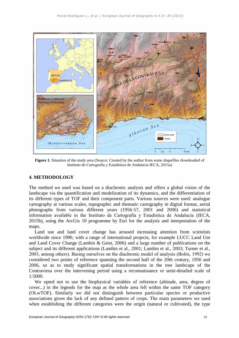
3. STUDY AREA
The Sierra de la Contraviesa is in the SE of the province of Granada and forms part of the
Penibetic coastal arc (see Figure 1). It is a medium altitude mountain range situated between
the Sierra Nevada and the Mediterranean Sea, down to which it descends directly with steep
slopes and an intricate hydrographic network. It has a dry Mediterranean climate, softened by
its altitude and the orientation of its slopes due to its north-south layout. It has poor skeletal
soils (eutric regosols, calcaric regosols and lithosols) affected by severe erosion processes
(Proyecto LUCDEME, 1987). It is covered by an original agro-forestry system dominated
above all by woody crops grown on non-irrigated land. In administrative terms, its area of
almost 600 km² covers 12 municipal areas (Sorvilán, Rubite, Polopos, Albuñol, Torvizcón,
Murtas, Albondón, Almegíjar, Cadiar, Cástaras, Lobras and Turón) either totally or partially,
and it has a population of about 14,000 people. In socioeconomic terms it is a marginal area
with an ageing population that has suffered drastic rural exodus (Remmers, 1998). For this
research we selected the village of Murtas, which has a municipal area of 72 km2 and 541
inhabitants (INE, 2014).
Porcel Rodriguez L., et al. / European Journal of Geography 6 4 21–34 (2015)
European Journal of Geography-ISSN 1792-1341 © All rights reserved 24
Figure 1. Situation of the study area (Source: Created by the author from some shapefiles downloaded of
Instituto de Cartografía y Estadística de Andalucia IECA, 2015a)
4. METHODOLOGY
The method we used was based on a diachronic analysis and offers a global vision of the
landscape via the quantification and modelization of its dynamics, and the differentiation of
its different types of TOF and their component parts. Various sources were used: analogue
cartography at various scales, topographic and thematic cartography in digital format, aerial
photographs from various different years (1956-57, 2001 and 2006) and statistical
information available in the Instituto de Cartografía y Estadística de Andalucía (IECA,
2015b), using the ArcGis 10 programme by Esri for the analysis and interpretation of the
maps.
Land use and land cover change has aroused increasing attention from scientists
worldwide since 1990, with a range of international projects, for example LUCC Land Use
and Land Cover Change (Lambin & Geist, 2006) and a large number of publications on the
subject and its different applications (Lambin et al., 2001; Lambin et al., 2003; Turner et al.,
2003, among others). Basing ourselves on the diachronic model of analysis (Bolós, 1992) we
considered two points of reference spanning the second half of the 20th century, 1956 and
2006, so as to study significant spatial transformations in the tree landscape of the
Contraviesa over the intervening period using a reconnaissance or semi-detailed scale of
1:5000.
We opted not to use the biophysical variables of reference (altitude, area, degree of
cover...) in the legends for the map as the whole area fell within the same TOF category
(OLwTOF). Similarly we did not distinguish between particular species or productive
associations given the lack of any defined pattern of crops. The main parameters we used
when establishing the different categories were the origin (natural or cultivated), the type
Porcel Rodriguez L., et al. / European Journal of Geography 6 4 21–34 (2015)
European Journal of Geography-ISSN 1792-1341 © All rights reserved 25
(herbaceous- woody) and the associations between types of crop (trees, mixed, herbaceous).
As a result in the legend we differentiate firstly between agricultural groundcovers, dividing
them into three subcategories (tree-covered, mixed, herbaceous) and secondly, groundcovers
of natural origin (small patches of wood). The main characteristics of these categories of TOF
are:
1) Small patch of woodland: this groundcover is made up natural vegetation with
arboreal stratum with a surface area of less than 0.5 ha thus meeting the definition of TOF
established by the FAO.
2) Herbaceous crops-vines: this form of groundcover combines different types of plant.
Although it is non-arboreal, we decided to consider it due to the historic importance of the
two crops in the study area in terms of surface area and local tradition, and due to the scarce
yet noteworthy presence of trees within them. These two apparently opposing types of crop
(herbaceous crops are annual while woody crops are permanent) were grouped together
because they are both very labour intensive and above all because of the difficulty in
distinguishing between them in the old photographs.
3) Mixed crops: this combined category groups together spaces in which there is a
productive association between tree crops and herbaceous/vines. These areas are rarely laid
out according to defined spatial patterns.
4) Tree crops: this category refers to areas wholly occupied by trees typically planted in
irregular low density distribution patterns, and covering a small percentage of the available
ground.
5. RESULTS
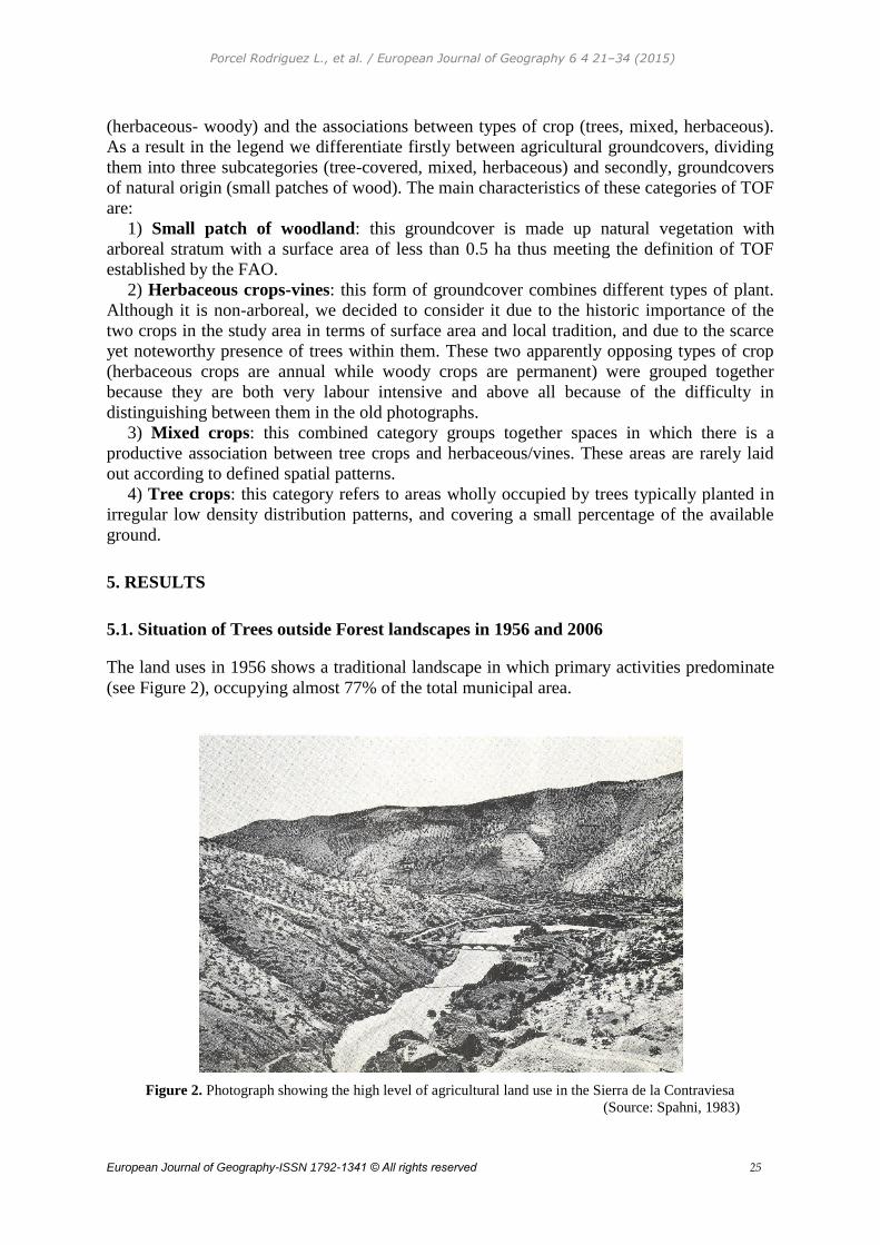
5.1. Situation of Trees outside Forest landscapes in 1956 and 2006
The land uses in 1956 shows a traditional landscape in which primary activities predominate
(see Figure 2), occupying almost 77% of the total municipal area.
Figure 2. Photograph showing the high level of agricultural land use in the Sierra de la Contraviesa
(Source: Spahni, 1983)
Porcel Rodriguez L., et al. / European Journal of Geography 6 4 21–34 (2015)
European Journal of Geography-ISSN 1792-1341 © All rights reserved 26
The three agricultural types of TOF differentiated in the map legend occupy similar
surface areas, albeit with a slight dominance of tree crops, which make up 31.12% of the total
(Table 1). The other two types of crop (herbaceous-vine and mixed crops) include a wide
array of cereal-based crops, which are of vital importance in an agrarian economy in which
people consume what they grow and have little interest in selling their produce on the market.
Groundcovers of natural origin such as the small patches of woodland occupy only 7% of
the total municipal area (see table) in places with very limited or no potential for agriculture.
Table 1. Land use according to types of TOF (1956)
Surface area (ha) % of municipal area
Patches of woodland 460.86 6.43
Scrub 1177.18 16.43
Tree Crops 2229.63 31.12
Herbaceous-Vine crops 1945.92 27.16
Mixed crops 1330.62 18.57
Built-up areas 19.41 0.27
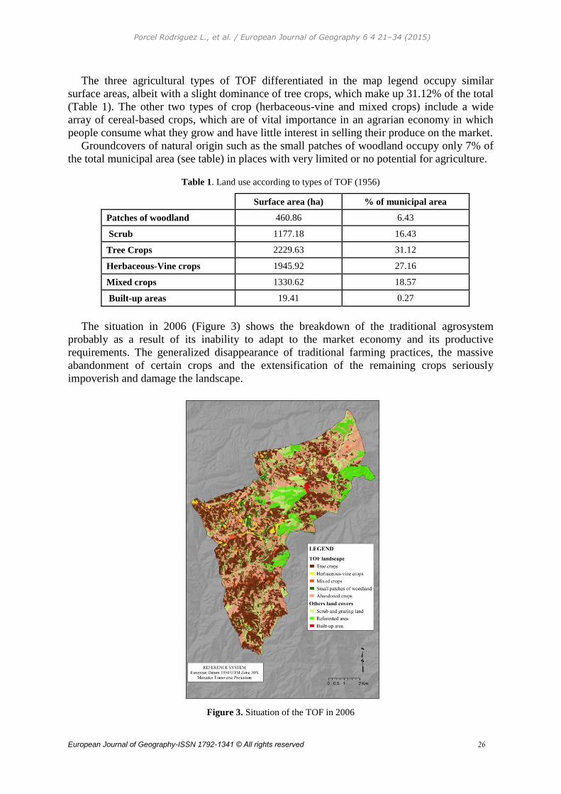
The situation in 2006 (Figure 3) shows the breakdown of the traditional agrosystem
probably as a result of its inability to adapt to the market economy and its productive
requirements. The generalized disappearance of traditional farming practices, the massive
abandonment of certain crops and the extensification of the remaining crops seriously
impoverish and damage the landscape.
Figure 3. Situation of the TOF in 2006
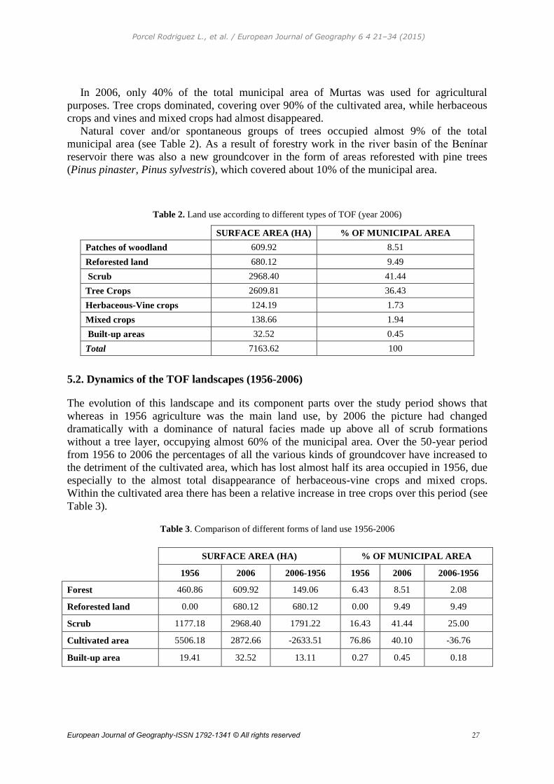
Porcel Rodriguez L., et al. / European Journal of Geography 6 4 21–34 (2015)
European Journal of Geography-ISSN 1792-1341 © All rights reserved 27
In 2006, only 40% of the total municipal area of Murtas was used for agricultural
purposes. Tree crops dominated, covering over 90% of the cultivated area, while herbaceous
crops and vines and mixed crops had almost disappeared.
Natural cover and/or spontaneous groups of trees occupied almost 9% of the total
municipal area (see Table 2). As a result of forestry work in the river basin of the Benínar
reservoir there was also a new groundcover in the form of areas reforested with pine trees
(Pinus pinaster, Pinus sylvestris), which covered about 10% of the municipal area.
Table 2. Land use according to different types of TOF (year 2006)
SURFACE AREA (HA) % OF MUNICIPAL AREA
Patches of woodland 609.92 8.51
Reforested land 680.12 9.49
Scrub 2968.40 41.44
Tree Crops 2609.81 36.43
Herbaceous-Vine crops 124.19 1.73
Mixed crops 138.66 1.94
Built-up areas 32.52 0.45
Total 7163.62 100
5.2. Dynamics of the TOF landscapes (1956-2006)
The evolution of this landscape and its component parts over the study period shows that
whereas in 1956 agriculture was the main land use, by 2006 the picture had changed
dramatically with a dominance of natural facies made up above all of scrub formations
without a tree layer, occupying almost 60% of the municipal area. Over the 50-year period
from 1956 to 2006 the percentages of all the various kinds of groundcover have increased to
the detriment of the cultivated area, which has lost almost half its area occupied in 1956, due
especially to the almost total disappearance of herbaceous-vine crops and mixed crops.
Within the cultivated area there has been a relative increase in tree crops over this period (see
Table 3).
Table 3. Comparison of different forms of land use 1956-2006
SURFACE AREA (HA) % OF MUNICIPAL AREA
1956 2006 2006-1956 1956 2006 2006-1956
Forest 460.86 609.92 149.06 6.43 8.51 2.08
Reforested land 0.00 680.12 680.12 0.00 9.49 9.49
Scrub 1177.18 2968.40 1791.22 16.43 41.44 25.00
Cultivated area 5506.18 2872.66 -2633.51 76.86 40.10 -36.76
Built-up area 19.41 32.52 13.11 0.27 0.45 0.18
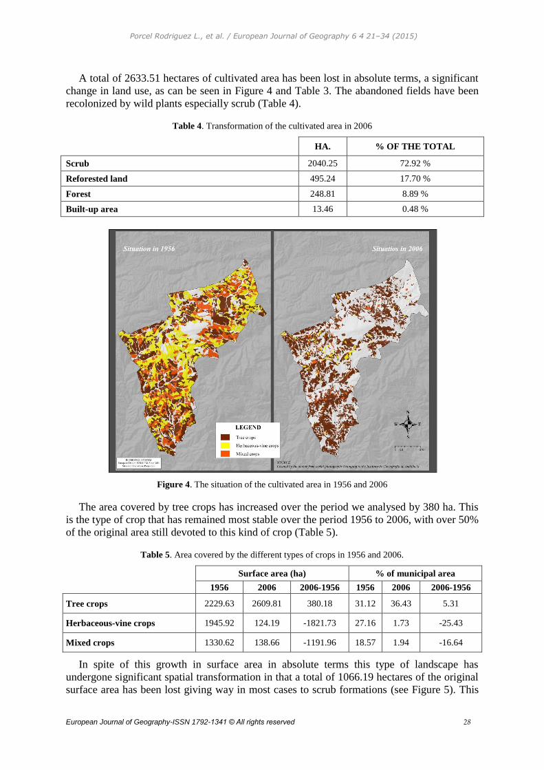
Porcel Rodriguez L., et al. / European Journal of Geography 6 4 21–34 (2015)
European Journal of Geography-ISSN 1792-1341 © All rights reserved 28
A total of 2633.51 hectares of cultivated area has been lost in absolute terms, a significant
change in land use, as can be seen in Figure 4 and Table 3. The abandoned fields have been
recolonized by wild plants especially scrub (Table 4).
Table 4. Transformation of the cultivated area in 2006
HA. % OF THE TOTAL
Scrub 2040.25 72.92 %
Reforested land 495.24 17.70 %
Forest 248.81 8.89 %
Built-up area 13.46 0.48 %
Figure 4. The situation of the cultivated area in 1956 and 2006
The area covered by tree crops has increased over the period we analysed by 380 ha. This
is the type of crop that has remained most stable over the period 1956 to 2006, with over 50%
of the original area still devoted to this kind of crop (Table 5).
Table 5. Area covered by the different types of crops in 1956 and 2006.
Surface area (ha) % of municipal area
1956 2006 2006-1956 1956 2006 2006-1956
Tree crops 2229.63 2609.81 380.18 31.12 36.43 5.31
Herbaceous-vine crops 1945.92 124.19 -1821.73 27.16 1.73 -25.43
Mixed crops 1330.62 138.66 -1191.96 18.57 1.94 -16.64
In spite of this growth in surface area in absolute terms this type of landscape has
undergone significant spatial transformation in that a total of 1066.19 hectares of the original
surface area has been lost giving way in most cases to scrub formations (see Figure 5). This
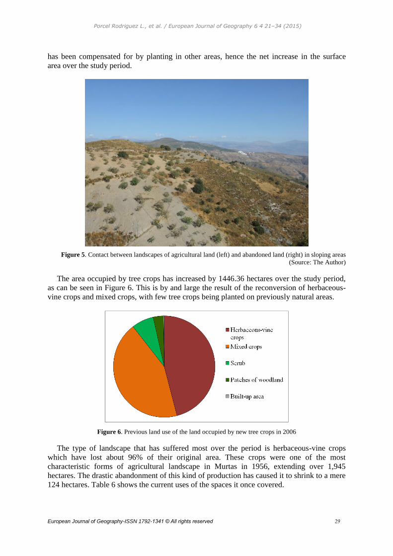
Porcel Rodriguez L., et al. / European Journal of Geography 6 4 21–34 (2015)
European Journal of Geography-ISSN 1792-1341 © All rights reserved 29
has been compensated for by planting in other areas, hence the net increase in the surface
area over the study period.
Figure 5. Contact between landscapes of agricultural land (left) and abandoned land (right) in sloping areas
(Source: The Author)
The area occupied by tree crops has increased by 1446.36 hectares over the study period,
as can be seen in Figure 6. This is by and large the result of the reconversion of herbaceous-
vine crops and mixed crops, with few tree crops being planted on previously natural areas.
Figure 6. Previous land use of the land occupied by new tree crops in 2006
The type of landscape that has suffered most over the period is herbaceous-vine crops
which have lost about 96% of their original area. These crops were one of the most
characteristic forms of agricultural landscape in Murtas in 1956, extending over 1,945
hectares. The drastic abandonment of this kind of production has caused it to shrink to a mere
124 hectares. Table 6 shows the current uses of the spaces it once covered.
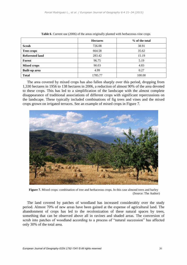
Porcel Rodriguez L., et al. / European Journal of Geography 6 4 21–34 (2015)
European Journal of Geography-ISSN 1792-1341 © All rights reserved 30
Table 6. Current use (2006) of the areas originally planted with herbaceous-vine crops
Hectares % of the total
Scrub 726.08 38.91
Tree crops 664.58 35.62
Reforested land 283.42 15.19
Forest 96.75 5.19
Mixed crops 90.03 4.83
Built-up area 4.99 0.27
Total 1785.77 100.00
The area covered by mixed crops has also fallen sharply over this period, dropping from
1,330 hectares in 1956 to 138 hectares in 2006, a reduction of almost 90% of the area devoted
to these crops. This has led to a simplification of the landscape with the almost complete
disappearance of traditional associations of different crops with significant repercussions on
the landscape. These typically included combinations of fig trees and vines and the mixed
crops grown on irrigated terraces. See an example of mixed crops in Figure 7.
Figure 7. Mixed crops: combination of tree and herbaceous crops. In this case almond trees and barley
(Source: The Author)
The land covered by patches of woodland has increased considerably over the study
period. Almost 70% of new areas have been gained at the expense of agricultural land. The
abandonment of crops has led to the recolonization of these natural spaces by trees,
something that can be observed above all in ravines and shaded areas. The conversion of
scrub into patches of woodland according to a process of “natural succession” has affected
only 30% of the total area.
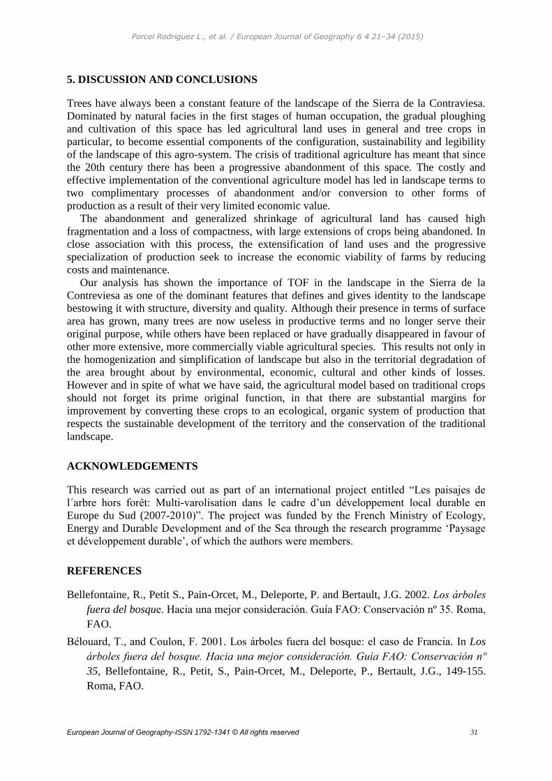
Porcel Rodriguez L., et al. / European Journal of Geography 6 4 21–34 (2015)
European Journal of Geography-ISSN 1792-1341 © All rights reserved 31
5. DISCUSSION AND CONCLUSIONS
Trees have always been a constant feature of the landscape of the Sierra de la Contraviesa.
Dominated by natural facies in the first stages of human occupation, the gradual ploughing
and cultivation of this space has led agricultural land uses in general and tree crops in
particular, to become essential components of the configuration, sustainability and legibility
of the landscape of this agro-system. The crisis of traditional agriculture has meant that since
the 20th century there has been a progressive abandonment of this space. The costly and
effective implementation of the conventional agriculture model has led in landscape terms to
two complimentary processes of abandonment and/or conversion to other forms of
production as a result of their very limited economic value.
The abandonment and generalized shrinkage of agricultural land has caused high
fragmentation and a loss of compactness, with large extensions of crops being abandoned. In
close association with this process, the extensification of land uses and the progressive
specialization of production seek to increase the economic viability of farms by reducing
costs and maintenance.
Our analysis has shown the importance of TOF in the landscape in the Sierra de la
Contreviesa as one of the dominant features that defines and gives identity to the landscape
bestowing it with structure, diversity and quality. Although their presence in terms of surface
area has grown, many trees are now useless in productive terms and no longer serve their
original purpose, while others have been replaced or have gradually disappeared in favour of
other more extensive, more commercially viable agricultural species. This results not only in
the homogenization and simplification of landscape but also in the territorial degradation of
the area brought about by environmental, economic, cultural and other kinds of losses.
However and in spite of what we have said, the agricultural model based on traditional crops
should not forget its prime original function, in that there are substantial margins for
improvement by converting these crops to an ecological, organic system of production that
respects the sustainable development of the territory and the conservation of the traditional
landscape.
ACKNOWLEDGEMENTS
This research was carried out as part of an international project entitled “Les paisajes de
l´arbre hors forêt: Multi-varolisation dans le cadre d’un développement local durable en
Europe du Sud (2007-2010)”. The project was funded by the French Ministry of Ecology,
Energy and Durable Development and of the Sea through the research programme ‘Paysage
et développement durable’, of which the authors were members.
REFERENCES
Bellefontaine, R., Petit S., Pain-Orcet, M., Deleporte, P. and Bertault, J.G. 2002. Los árboles
fuera del bosque. Hacia una mejor consideración. Guía FAO: Conservación nº 35. Roma,
FAO.
Bélouard, T., and Coulon, F. 2001. Los árboles fuera del bosque: el caso de Francia. In Los
árboles fuera del bosque. Hacia una mejor consideración. Guía FAO: Conservación nº
35, Bellefontaine, R., Petit, S., Pain-Orcet, M., Deleporte, P., Bertault, J.G., 149-155.
Roma, FAO.
Porcel Rodriguez L., et al. / European Journal of Geography 6 4 21–34 (2015)
European Journal of Geography-ISSN 1792-1341 © All rights reserved 32
Bolós i Capdevilla, M. 1992. Manual de Ciencia del Paisaje. Teoría, métodos y aplicaciones.
Barcelona: Ed. Masson.
Caballero Calvo, A. and Jiménez Olivencia, Y. 2013. Evaluación de recursos locales: Los
paisajes del árbol fuera del bosque en el municipio de Válor. In Desarrollo Local en
tiempos de crisis. ¿El retorno de los recursos endógenos?, coord. Rodríguez Martínez,
F., 279- 293. Granada: Universidad de Granada.
Camacho Olmedo, M.T. 1995. Cartografía de los paisajes erosivos de la Sierra de la
Contraviesa (provincias de Granada y Almería). Granada: Universidad de Granada.
Chavarría Sacasa, M.R. 2001. Arboles fuera del bosque en Nicaragua. In Proyecto
Información y análisis para el manejo forestal sostenible: Integrando esfuerzos
nacionales e internacionales en 13 Países tropicales en America Latina
(GCP/RLA/133/EC). Chile: FAO.
Comisión Europea. 1991. Medio Ambiente en Europa. El Informe Dobrís. Grupo de Trabajo
de la Agencia Europea de Medio Ambiente, DG XI & PHARE. Luxemburgo: Oficina de
Publicaciones de las Comunidades Europeas.
Corona, P., Chiriacò, M.V., Salvati, R., Marchett, M., Lasserre, B. and Ferrari, B. 2009.
Proposta metodologica per l’inventario su vasta scala degli alberi fuori foresta. Italian
Journal of Forest and Mountain Environments: 64 (6): 367-380.
Dogra, A. S. 2011. Contribution of Trees Outside Forests Toward Wood Production and
Environmental Amelioration. Indian Journal of Ecology: 38 (Special Issue): 1-5.
Foresta, H., Somarriba, E., Temu, A., Boulanger, D., Feuilly, H. and Gauthier, M. 2013.
Towards the Assessment of Trees Outside Forests. Resources Assessment Working Paper
183. Rome: FAO.
Garcia Manrique E. 1973. El viñedo en la costa Alpujarreña. Estudios geográficos: vol. 34 nº
132-133: 501-538.
Guillerme S., Alet B., Briane G., Coulon F.and Maire E. 2009. L’arbre hors forêt en France.
Anciens usages et nouvelles perspectives. Revue Forestière Française: 5 nº spécial Les
nouveaux usages de l’arbre: 543-560.
Guillerme S., Jiménez, Y. and Moreno, D. 2013. Les paysages d´arbres hors forêt, des
paysages porteurs des enjeux du développement durable. In Paysage et développement
durable, coor. Y. Luginbühl & D. Terrasson, 37-47. France: Editions Quae.
Guillerme, S., Jiménez, Y. and Moreno, D. 2015. Landscape of non-woodland trees:
landscapes which reveal the challenges of sustainable development. In Landscape and
Sustainable Development: The French Perspective, coor. Y. Luginbühl, D. Terrasson &
P. Howard, 27-36. UK: Ashgate Publishing.
Instituto de Cartografía y Estadística de Andalucia (IECA). 2015a. DERA. Datos Espaciales
de Referencia de Andalucía para escalas intermedias. Sevilla: Consejería de Economía,
Innovación, Ciencia y Empleo.
Porcel Rodriguez L., et al. / European Journal of Geography 6 4 21–34 (2015)
European Journal of Geography-ISSN 1792-1341 © All rights reserved 33
Instituto de Cartografía y Estadística de Andalucia (IECA). 2015b. Localizador de
Información Espacial de Andalucía. Last access june 2015. Available in
http://www.juntadeandalucia.es/institutodeestadisticaycartografia/lineav2/web/
Instituto Nacional de Estadística (INE). 2014. Encuesta de Población Activa. Last access may
2015.Available in http://www.ine.es/dynt3/inebase/es/index.html?padre=517&dh=1
Inventaire Forestier National (IFN). 2000. Les arbres hors forêts en France - une ressource
inféodée à l'agriculture. A case study in contribution to the FAO Forest Resource
Assessment Programme. Rome: FAO.
Kleinn, C. 2000. On large-area inventory and assessment of trees outside the forest.
Unasylva, 200(51): 3-10.
Lambin, E. and Geist, F. 2006. Land-use and Land-cover change. Berlin: Springer-Verlag.
Lambin, E.F., Geist, H.J. and Lepers, E. 2003. Dynamics of land-use and land-cover change
in tropical regions. Annual Review of Environment and Resources: vol. 28: 205-241.
Lambin, E.F., Turner, B.L., Geist, H.J. et al. 2001. The causes of land-use and land-cover
change: moving beyond the myths. Global Environmental Change: vol. 11, nº 4: 261-
269.
Muñoz Rodríguez, T. 2001. Arboles fuera del bosque en Bolivia. In Proyecto Información y
análisis para el manejo forestal sostenible: Integrando esfuerzos nacionales e
internacionales en 13 Países tropicales en America Latina (GCP/RLA/133/EC). Chile:
FAO.
Pandey, D. 2008. Trees Outside the Forest (TOF) Resources in India. International Forestry
Review: 10(2): 125-133.
Petit-Berghem, Y. 2012. L’arbre hors forêt en domaine littoral (ouest de la France) : mise en
scène de l’objet, gestion et patrimonialisation. Vertigo-la revue électronique en sciences
de l'environnement: Volume 12, nº 1: Online.
Pointereau, P. and Bazile, D. 1995. L’arbre des champs: haies, alignements et présvergers ou
l’art du bocage. Toulouse: Editions Solagro.
Porcel Rodríguez, L. and Jiménez Olivencia, Y. 2013a. Hacia una metodología aplicada a la
evaluación y seguimiento de los recursos paisajísticos locales. In Desarrollo Local en
tiempos de crisis. ¿El retorno de los recursos endógenos?, coord. Rodríguez Martínez,
F., 297-317. Granada: Universidad de Granada.
Porcel Rodríguez, L. and Jiménez Olivencia, Y. 2013b. Los paisajes del árbol fuera del
bosque en el contexto del desarrollo local sostenible: el caso de los policultivos de sierra
en el valle del río Lanjarón (Sierra Nevada). In Desarrollo Regional Sostenible en
tiempos de crisis, ed. Camacho Ballesta, J.A. y Jiménez Olivencia, Y., nº. 2, 201-224.
Granada: Universidad de Granada.
Proyecto Lucdeme. 1987. Mapa de suelos escala 1:100.000. Albuñol hoja nº 1056. Madrid:
Ministreio de Agricultura, Pesca y Almnentación and ICONA.
Porcel Rodriguez L., et al. / European Journal of Geography 6 4 21–34 (2015)
European Journal of Geography-ISSN 1792-1341 © All rights reserved 34
Remmers, G.A. 1998. Con cojones y maestría : un estudio sociológico-agronómico acerca del
desarrollo rural endógeno y procesos de localización en la Sierra de la Contraviesa
(España). Amsterdam: Thela Publishers
Rivas Martínez, S. 1986. Memoria del Mapa de series de vegetación de España. Madrid: Ed.
ICONA, Ministerio Agricultura, Pesca y Alimentación.
Rodríguez Martínez, F. 1985. Granada: medio físico y desarrollo. Granada: Servicio de
Publicaciones de la Universidad de Granada.
Sedjo, R.A. 1999. The potential of high-yield plantation forestry for meeting timber needs.
New Forests: 17: 339-359.
Singh C.D. 2000. Valuation and evaluation of trees outside the forest (TOF) of Bangladesh.
Draft paper for a regional study for Asia and Pacific in contribution to the Forest
Resource Assessment (FRA) 2000. Rome: FAO.
Spahni, J.C. 1983. La Alpujarra, la Andalucía secreta. Granada: Diputación Provincial de
Granada.
Thaman, R.R. 2002. Trees outside forests as a foundation for sustainable development in the
Small Island Developing States of the Pacific Ocean. International Forestry Review,
Volume 4, Nº 4: 268-276.
Turner, M.G., Pearson, S.M., Bolstad, P. and Wear, D.N. 2003. Effects of land-cover change
on spatial pattern of forest communities in the Southern Appalachian Mountains (USA).
Landscape Ecology:, nº18: 449–464.
European Journal of Geography Volume 6, Number 4: 35 - 50, December 2015
©Association of European Geographers
European Journal of Geography-ISSN 1792-1341 © All rights reserved 35
ASSESSING SUSTAINABILITY IN COASTAL TOURISM SECTORS OF ODISHA
COAST, INDIA.
Nilay Kanti BARMAN
Department of Geography, Hijli College, Kharagpur -721306, Paschim Medinipur, West Bengal, India
Goutam BERA Dept. of Geography and Environment Management, Vidyasagar University, Midnapore-721102, Paschim
Medinipur, West Bengal, India
Mihir Kumar PRADHAN
Department of Geography and Environment Management, Vidyasgar University, Midnapore-721102, Paschim
Medinipur, West Bengal, India
Abstract
Balasore is famous for its long sea beach and pleasant natural beauty. This district is noted
for the river Subarnarekha, Buhdabalanga and also the extended calm sea beach. It is also
bestowed with the Chandipur, Talsari and Bichitrapur sea Beach. Balasore is appreciated for
its salt, Brass utensils, stone and clay works. Ayodhya, Balaramgadi, Bardhanpur,
Bhusandeswar, Chandaneswar, Chandipur, Kasaphal, Langaleswar, Laxmannath,
Panchalingeswar, Raibania, Remuna, Sajanagarh, Talasari, Tripisagadia and Kupari are some
of the places of tourist interest. The sustainable development as a strategic tool requires a
process of planning and management that brings together a series of interests and indigenous
people’s concerns in the form of planning and development. The objective of this present
research is to study the indigenous people’s attitude in Coastal tract of Balasore district,
Odisha- towards the impacts of coastal tourism as also to suggest the strategic interventions
for current problems and future needs through intensive field survey and human perception
survey with the help of some statistical methods and GIS tools. The study finding suggests
that the residents’ participation and co-operation is necessary to make the tourism
development more sustainable.
Keywords: sustainable tourism development, coastal tract, human perception, indigenous people
1. INTRODUCTION
Our country has a long coastline of about 7500 km including that of its island territories. The
coastal zone of India is under increasing pressure due to rapid urbanization, tourism
development, discharge of waste effluents, municipal sewage, over exploitation of coastal
resources and continued development in hazard prone areas. There are many studies on
coastal tourism emphasize on the tourism system rather than on the interaction of the tourism
and related environmental systems (Wong,P.P, 1993). Low-lying delta, low-elevation reef
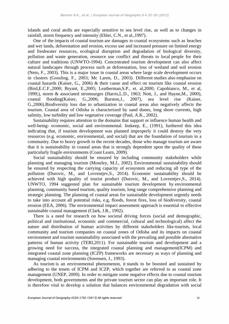
Barman N.K., et al. / European Journal of Geography 6 4 35–50 (2015)
European Journal of Geography-ISSN 1792-1341 © All rights reserved 36
islands and coral atolls are especially sensitive to sea level rise, as well as to changes in
rainfall, storm frequency and intensity (Ehler, C.N., et al.,1997).
One of the impacts of coastal tourism are damages to coastal ecosystems such as beaches
and wet lands, deforestation and erosion, excess use and increased pressure on limited energy
and freshwater resources, ecological disruption and degradation of biological diversity,
pollution and waste generation, resource use conflict and threats to local people for their
culture and traditions (UNWTO-1994). Concentrated tourism development can also affect
natural landscapes through process such as deforestation, loss of wetland and soil erosion
(Neto, F., 2003). This is a major issue in coastal areas where large scale development occurs
in clusters (Gossling, F., 2003; Mc Laren, D., 2003). Different studies also emphasise on
coastal hazards (Kaiser, G., 2006) & their cause and effect on tourism like coastal erosion
(Bird,E.C.F.,2000; Bryant, E.,2005; Leatherman,S.P., et. al,2000; Capobianco, M., et al,
1999;), storm & associated stromsurges (Harris,L.D., 1963; Nott, J., and Hayne,M., 2000),
coastal flooding(Kaiser, G.,2006; Burston,J., 2007), sea level rise (Kaiser,
G.,2006).Biodiversity loss due to urbanization in coastal areas also negatively affects the
tourism. Coastal area of Odisha is characterized by sand dunes, long shore currents, high
salinity, low turbidity and low vegetative coverage (Paul, A.K., 2002).
Sustainability requires attention to the domains that support or influence human health and
well-being- economic, social and environmental. Inskeep, E., (1991), furthered this idea
indicating that, if tourism development was planned improperly it could destroy the very
resources (e.g. economic, environmental, and social) that are the foundation of tourism in a
community. Due to heavy growth in the recent decades, those who manage tourism are aware
that it is sustainability in coastal areas that is strongly dependent upon the quality of these
particularly fragile environments (Coast Learn, 2009).
Social sustainability should be ensured by including community stakeholders while
planning and managing tourism (Moseley, M.J., 2002). Environmental sustainability should
be ensured by respecting the carrying capacity of ecosystem and reducing all type of the
pollution (Durovic, M., and Lovrentjev,S., 2014). Economic sustainability should be
achieved with high quality of tourist product (Durovic, M., and Lovrentjev,S., 2014).
UNWTO, 1994 suggested plan for sustainable tourism development by environmental
planning, community based tourism, quality tourism, long range comprehensive planning and
strategic planning. The planning of coastal areas for sustainable development urgently needs
to take into account all potential risks, e.g, floods, forest fires, loss of biodiversity, coastal
erosion (EEA, 2006). The environmental impact assessment approach is essential to effective
sustainable coastal management (Clark, J.R., 1992).
There is a need for research on how societal driving forces (social and demographic,
political and institutional, economic and commercial, cultural and technological) affect the
nature and distribution of human activities by different stakeholders like-tourists, local
community and tourism companies on coastal zones of Odisha and its impacts on coastal
environment and tourism sustainability associated with the prevailing and possible alternative
patterns of human activity (TERI,2011). For sustainable tourism and development and a
growing need for success, the integrated coastal planning and management(ICPM) and
integrated coastal zone planning (ICZP) frameworks are necessary as ways of planning and
managing coastal environments (Sorensen, J., 1993).
As tourism is an environmental phenomenon, it stands to be boosted and sustained by
adhering to the tenets of ICPM and ICZP, which together are referred to as coastal zone
management (UNEP, 2009). In order to mitigate some negative effects due to coastal tourism
development, both governments and the private tourism sector can play an important role. It
is therefore vital to develop a solution that balances environmental degradation with social
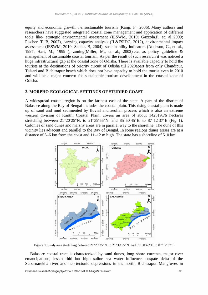
Barman N.K., et al. / European Journal of Geography 6 4 35–50 (2015)
European Journal of Geography-ISSN 1792-1341 © All rights reserved 37
equity and economic growth, i.e. sustainable tourism (Kanji, F., 2006). Many authors and
researchers have suggested integrated coastal zone management and application of different
tools like- strategic environmental assessment (IESWM, 2010; Gazzola.P, et. al.,2009;
Fischer. T. B, 2007), carrying capacity analysis (IL&FSIDC, 2012), environmental impact
assessment (IESWM, 2010; Sadler. B, 2004), sustainability indicators (Atkisson, G., et. al.,
1997; Hart, M., 1999 ), zoning(Miller, M., et. al., 2002) etc. as policy guideline &
management of sustainable coastal tourism. As per the result of such research it was noticed a
huge infrastructural gap at the coastal zone of Odisha. There is available capacity to hold the
tourists at the destinations of priority circuit of Odisha till 2020apart from only Chandipur,
Talsari and Bichitrapur beach which does not have capacity to hold the tourist even in 2010
and will be a major concern for sustainable tourism development in the coastal zone of
Odisha.
2. MORPHO-ECOLOGICAL SETTINGS OF STUDIED COAST
A widespread coastal region is on the farthest east of the state. A part of the district of
Balasore along the Bay of Bengal includes the coastal plain. This rising coastal plain is made
up of sand and mud sedimented by fluvial and aeolian process which is also an extreme
western division of Kanthi Coastal Plain, covers an area of about 142519.76 hectares
stretching between 212025N. to 213955N. and 855045E. to 871237E (Fig 1).
Colonies of sand dunes and marshy areas are in parallel way to the shoreline. The dune of this
vicinity lies adjacent and parallel to the Bay of Bengal. In some regions dunes arises are at a
distance of 5–6 km from the coast and 11–12 m high. The state has a shoreline of 510 km.
Figure 1. Study area stretching between 212025N. to 213955N. and 855045E. to 871237E
Balasore coastal tract is characterized by sand dunes, long shore currents, major river
emancipations, less turbid but high saline sea water influence, cuspate delta of the
Subarnarekha river and neo-tectonic depressions in the north. Bichitrapur Mangroves in
Barman N.K., et al. / European Journal of Geography 6 4 35–50 (2015)
European Journal of Geography-ISSN 1792-1341 © All rights reserved 38
Balasore district has a complicated coastline, bunches of early growing deltas with
interlinked tidal creeks, and estuary. Deltaic expanses are generally clayey due to high
deposit of sediments through the Subarnarekha system. A clayey bedspread covering gravels
of sandstone, siltstone and quartz designate quaternary era of the area. Consequently, Odisha
does not acquire the fertile alluvium as before and the topography is not de-salinated by river
floods. The wide beaches and intensive network of inlets and creeks, mangrove swamps,
mudflats, frequent coastal dunes and sand flats are the major characteristics of this coastal
region.
3. METHODS AND MATERIALS
The following techniques, tools and methods are projected to categorize the coastal
area that is influenced the most and appraise the future condition of coast if such type of trend
in coastal development occurs:
3.1 Data Collection, Questionnaires, Interviews and Analysis
To construct a methodical categorization of coastal zone, to achieve objective based study
and to find most favorable solution, the integrated use of modern techniques and tools such
as Geographic Information Systems (GIS), Image Processing Systems (IPS), Remote
Sensing (RS) with Rapid Impact Assessment Matrix and SWOT analysis to be a talented
implementation and would address in representing sustainable coastal tourism industries
development in the coast of Balasore, Odisha.
SWOT analysis instigated in the 1960s (Dyson,R.G., 2004) and is generally used in the
development of marketing plans and decision support (Bbernroider, E., 2002;Chang, H.H.,
and Huang, W.C., 2006;Houben, G., Lenie K., and Vanhoof, K., 1999) is hardly ever uses
for any coastal morphological sustainability with few studies known (Nouri, J., Karbassi,
A.R., and Mirkia, S., 2008; Sanò, M., and Fierro, G., 2003). In recent times the SWOT
analysis has achieved wider fields of application and it is usually used to recognize features
and to resolve divergence of the terrain.
The perception of the Rapid Impact Assessment Matrix (RIAM) to appraise the human
cause and development to hurriedly changing coastal environment is a promising
assessment tool to study the status of Balasore coast and its vulnerability. RIAM is developed
by DHI Water, Environment & Health to support in the preparation of an Environmental
Impact Assessment (EIA). RIAM permits full precision of the decisions made in an
evaluation study (Pastakia, C.M.R., 1998). The RIAM system is based on
straightforward perceptions and has been experienced in a number of diverse conditions. It is
a very influential tool in connection with EIA’s and was hardened on various project studies
(Jensen, K., 1998) where a multidisciplinary squad approach is used (Morris, P., and
Biggs, J., 1995). It receives in data from different environmental, social and economic
segments connected with coastal zone to be analyzed against common
significant criteria within a common matrix, thus providing a hurried, clear estimation of
the major impacts on the coasts. It represents the scoring within a matrix that has been
intended to allow subjective judgments to be quantitatively recorded for appraisal of coastal
environmental changes of Balasore coast, Odisha in relation to a variety of developmental
projects regarding the customary coastal resource uses along the coast. Coastal Landscape,
Geomorphologic and coastline change may be understood through a comparative analysis of
the spatial and temporal changes took place in the coast of Balasore through a long duration
Barman N.K., et al. / European Journal of Geography 6 4 35–50 (2015)
European Journal of Geography-ISSN 1792-1341 © All rights reserved 39
of time through taking out information from remotely sensed data and combination of GIS.
4. PREMISES OF THE STUDY
The above mentioned techniques, tools and methods are projected for the study on the
basis of the following hypotheses:
Anthropogenic uses of coastal resources in the coastal stretches are the most
important criteria that are causing coastal alteration of geomorphology or
coastline apart from the natural process.
Least managed, unscientific and nontechnical use of coastal resources will remain
growing in the next decade if it’s not switched correctly with
sufficient scientific research based information. This puts in more pressure on
Balasore’s coastal area in general and aquatic resources in particular.
If such kind of trend of development is going on in the coastal region, it is estimated
in the near future there will not be any coastal region left untouched in Balasore.
The techniques which are mentioned above can emphasize the problem, cause and
clarification in a more persuasive approach in provisos of more reliable scientific
information.
5. RESULTS AND DISCUSSION
Tourism Interfaces in Balasore Coast
It is clear that the “Tourism Sector” builds up much more job opportunities in comparison
with any other sector in terms of per million rupees investment. The district Balasore is no
exception. Because of sea side location and cultural heritage, there is a vast scope for the
expansion of tourism in this district and to obtain this, the state government and the local
administration have to set up mission and vision. The private agencies should be used as a
part of this mission and vision. The district Balasore is a miniature form of the state Odisha in
terms of culture, tourism, literature, architecture, heritage, natural wonders and religious
momentum. So its popularity crosses the limits of the nation. From time immemorial the
faunal and floral community, it’s history, geographical location and culture has invited the
people of nation and from the outside of its boundaries. The district Balasore is called “The
Germany of Odisha” due to the sea facing situation in the north, the river network, blue hills
and extensive meadow and for extraordinary beautiful beach. The name of the district
‘Balasore’ is chosen after the name of “Lord Baleswar”. Its archaeological structure is
excellent. Its temple, wild life, ruined monuments; quaint little hilly picnic spot helped her to
be an ideal tourist spot.
In the whole district of Balasore there are 19 major tourist spots (Table 1). 10 among which
are included in the present study area (Fig. 2).
Table 1. List of major tourist centers in Balasore District
Place Importance
Ayodhya Religious centre and archaeological site
Balaramgadi Sea beach and fish trading centre
Balasore Urban area
Bardhanpur Religious centre
Bhusandeswar Religious centre
Barman N.K., et al. / European Journal of Geography 6 4 35–50 (2015)
European Journal of Geography-ISSN 1792-1341 © All rights reserved 40
Chandaneswar Religious centre
Chandipur Beautiful beach
Chasakhanda Baghajatin memorial
ChoumukhDagra Sea beach
Inchudi Historical (Freedom movement)
Kasaphal Sea beach
Kupari Religious centre
Langaleswar Religious centre
Laxmannath Welcome point
Panchalingeswar Religious centre and scenic spot
Raibania Fort
Remuna Religious centre
Sajanagar Religious centre
Talsari Sea beach
Tripisagadia Religious centre
Source: Comprehensive district annual plan 2011-2012(Balasore)
Chandipur
The beach of Chandipur is very wide, golden and calm. The sea water advances towards the
shore as much 5 km at the time of high tide and retreat the same during low ebb. In addition
to this the huge sand banks, wild creepers, the rusting of the branches of casuarinas trees
along with the rhythmic dance of both ebbs are enough to create obsession among the
tourists.
Langaleswar
This place is situated by the river ‘Parbati’. The mythology and local belief said that Lord
Shiva ploughed the land himself for cultivation and so the name “Langaleswar” is given.
Daily worship is the feature of this area and so a large number of followers come here every
day.
Kashafal
It is an ideal fishing harbor. Two rivers Dubdubi and Panchapali meet here and flow into the
Bay of Bengal. There is the scope of boating in these two rivers. No nature lover cannot but
fell in love of the calm, green village atmosphere and the deep forest of casuarinas of this
place.
Chandaneswar and Talsari
The temple of Lord Chandaneswar is located here. It is a very sacred religious place. Many
pilgrims from West Bengal come to visit this holy place apart from the peoples of Balasore.
Daily worship and ‘Gajan’ at the end of the Bengali year are observed here. From here a road
runs 5 km away towards the Bay of Bengal where the place Talsari is situated. It is mainly a
fishing harbor but the big sand dunes, the confluence of the Jatranala and whispering of the
enclaves of casuarinas are the points of attractions. The sea bath is very interesting along with
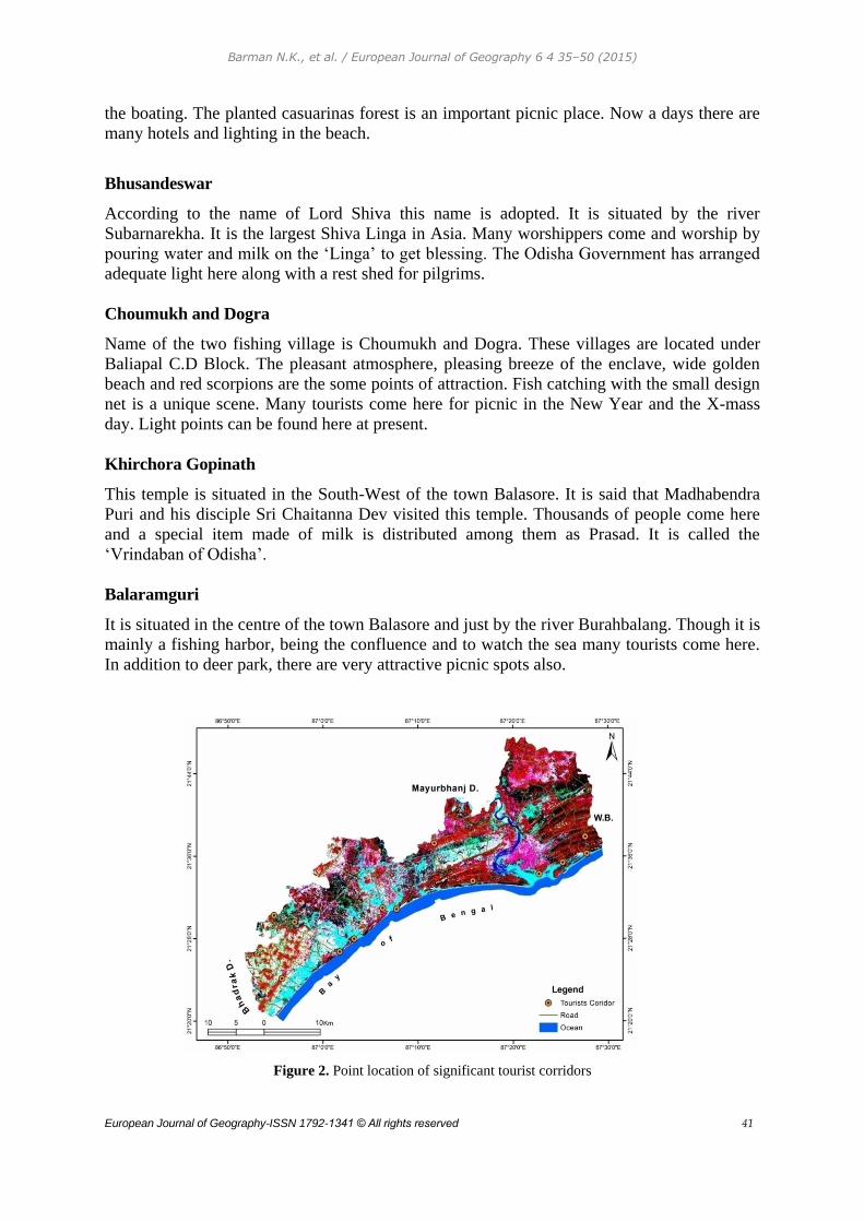
Barman N.K., et al. / European Journal of Geography 6 4 35–50 (2015)
European Journal of Geography-ISSN 1792-1341 © All rights reserved 41
the boating. The planted casuarinas forest is an important picnic place. Now a days there are
many hotels and lighting in the beach.
Bhusandeswar
According to the name of Lord Shiva this name is adopted. It is situated by the river
Subarnarekha. It is the largest Shiva Linga in Asia. Many worshippers come and worship by
pouring water and milk on the ‘Linga’ to get blessing. The Odisha Government has arranged
adequate light here along with a rest shed for pilgrims.
Choumukh and Dogra
Name of the two fishing village is Choumukh and Dogra. These villages are located under
Baliapal C.D Block. The pleasant atmosphere, pleasing breeze of the enclave, wide golden
beach and red scorpions are the some points of attraction. Fish catching with the small design
net is a unique scene. Many tourists come here for picnic in the New Year and the X-mass
day. Light points can be found here at present.
Khirchora Gopinath
This temple is situated in the South-West of the town Balasore. It is said that Madhabendra
Puri and his disciple Sri Chaitanna Dev visited this temple. Thousands of people come here
and a special item made of milk is distributed among them as Prasad. It is called the
‘Vrindaban of Odisha’.
Balaramguri
It is situated in the centre of the town Balasore and just by the river Burahbalang. Though it is
mainly a fishing harbor, being the confluence and to watch the sea many tourists come here.
In addition to deer park, there are very attractive picnic spots also.
Figure 2. Point location of significant tourist corridors
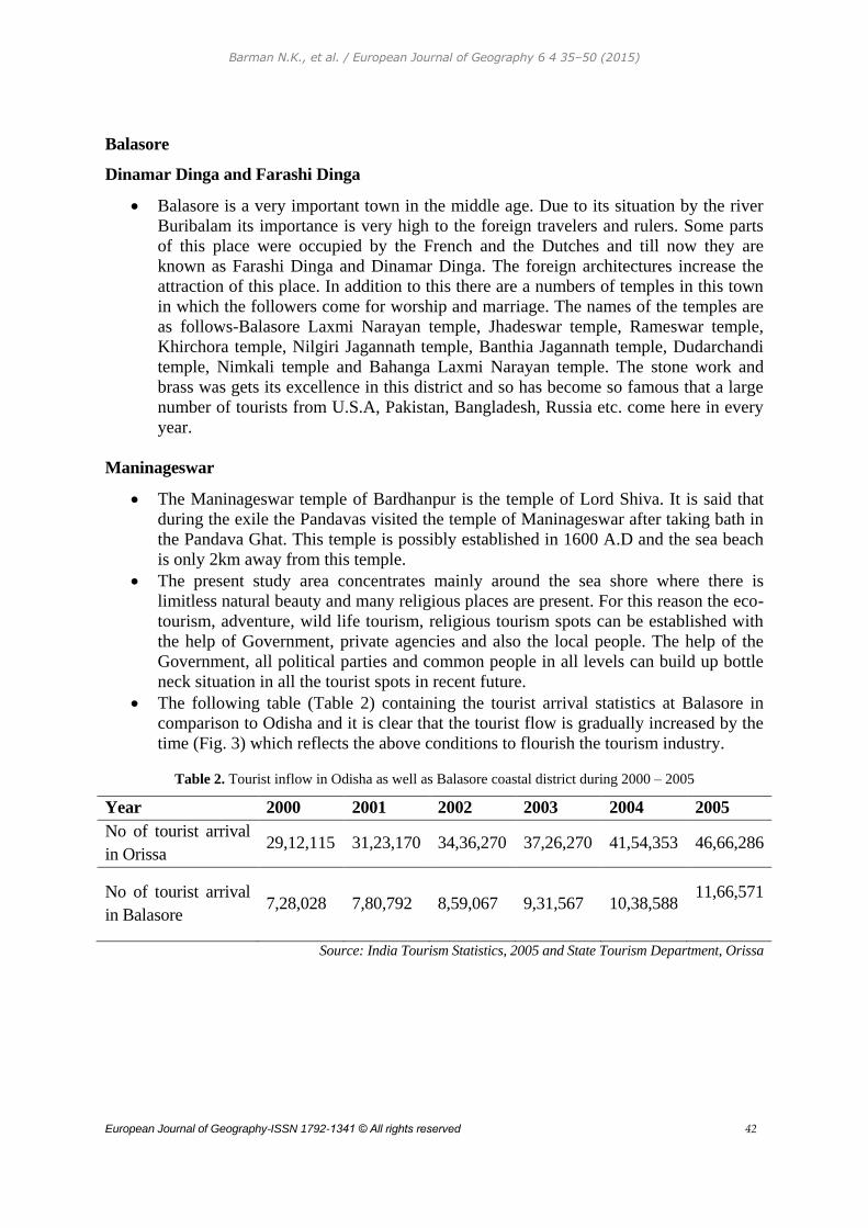
Barman N.K., et al. / European Journal of Geography 6 4 35–50 (2015)
European Journal of Geography-ISSN 1792-1341 © All rights reserved 42
Balasore
Dinamar Dinga and Farashi Dinga
Balasore is a very important town in the middle age. Due to its situation by the river
Buribalam its importance is very high to the foreign travelers and rulers. Some parts
of this place were occupied by the French and the Dutches and till now they are
known as Farashi Dinga and Dinamar Dinga. The foreign architectures increase the
attraction of this place. In addition to this there are a numbers of temples in this town
in which the followers come for worship and marriage. The names of the temples are
as follows-Balasore Laxmi Narayan temple, Jhadeswar temple, Rameswar temple,
Khirchora temple, Nilgiri Jagannath temple, Banthia Jagannath temple, Dudarchandi
temple, Nimkali temple and Bahanga Laxmi Narayan temple. The stone work and
brass was gets its excellence in this district and so has become so famous that a large
number of tourists from U.S.A, Pakistan, Bangladesh, Russia etc. come here in every
year.
Maninageswar
The Maninageswar temple of Bardhanpur is the temple of Lord Shiva. It is said that
during the exile the Pandavas visited the temple of Maninageswar after taking bath in
the Pandava Ghat. This temple is possibly established in 1600 A.D and the sea beach
is only 2km away from this temple.
The present study area concentrates mainly around the sea shore where there is
limitless natural beauty and many religious places are present. For this reason the eco-
tourism, adventure, wild life tourism, religious tourism spots can be established with
the help of Government, private agencies and also the local people. The help of the
Government, all political parties and common people in all levels can build up bottle
neck situation in all the tourist spots in recent future.
The following table (Table 2) containing the tourist arrival statistics at Balasore in
comparison to Odisha and it is clear that the tourist flow is gradually increased by the
time (Fig. 3) which reflects the above conditions to flourish the tourism industry.
Table 2. Tourist inflow in Odisha as well as Balasore coastal district during 2000 – 2005
Year 2000 2001 2002 2003 2004 2005
No of tourist arrival
in Orissa 29,12,115 31,23,170 34,36,270 37,26,270 41,54,353 46,66,286
No of tourist arrival
in Balasore 7,28,028 7,80,792 8,59,067 9,31,567 10,38,588
11,66,571
Source: India Tourism Statistics, 2005 and State Tourism Department, Orissa
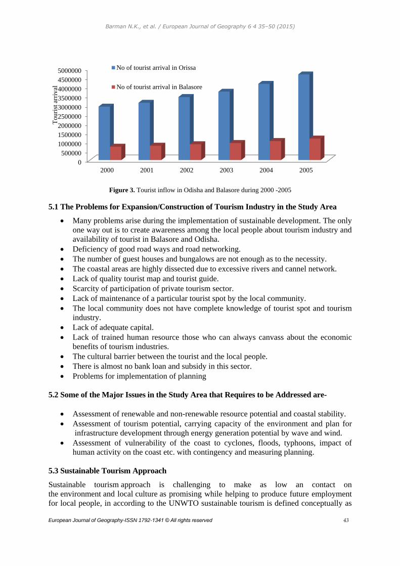
Barman N.K., et al. / European Journal of Geography 6 4 35–50 (2015)
European Journal of Geography-ISSN 1792-1341 © All rights reserved 43
Figure 3. Tourist inflow in Odisha and Balasore during 2000 -2005
5.1 The Problems for Expansion/Construction of Tourism Industry in the Study Area
Many problems arise during the implementation of sustainable development. The only
one way out is to create awareness among the local people about tourism industry and
availability of tourist in Balasore and Odisha.
Deficiency of good road ways and road networking.
The number of guest houses and bungalows are not enough as to the necessity.
The coastal areas are highly dissected due to excessive rivers and cannel network.
Lack of quality tourist map and tourist guide.
Scarcity of participation of private tourism sector.
Lack of maintenance of a particular tourist spot by the local community.
The local community does not have complete knowledge of tourist spot and tourism
industry.
Lack of adequate capital.
Lack of trained human resource those who can always canvass about the economic
benefits of tourism industries.
The cultural barrier between the tourist and the local people.
There is almost no bank loan and subsidy in this sector.
Problems for implementation of planning
5.2 Some of the Major Issues in the Study Area that Requires to be Addressed are-
Assessment of renewable and non-renewable resource potential and coastal stability.
Assessment of tourism potential, carrying capacity of the environment and plan for
infrastructure development through energy generation potential by wave and wind.
Assessment of vulnerability of the coast to cyclones, floods, typhoons, impact of
human activity on the coast etc. with contingency and measuring planning.
5.3 Sustainable Tourism Approach
Sustainable tourism approach is challenging to make as low an contact on
the environment and local culture as promising while helping to produce future employment
for local people, in according to the UNWTO sustainable tourism is defined conceptually as
0
500000
1000000
1500000
2000000
2500000
3000000
3500000
4000000
4500000
5000000
2000 2001 2002 2003 2004 2005
To
uri
st a
rriv
al
No of tourist arrival in Orissa
No of tourist arrival in Balasore
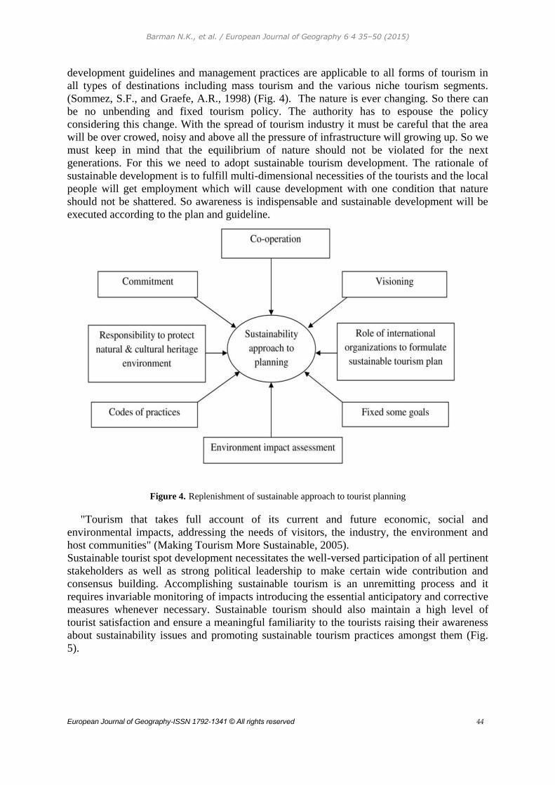
Barman N.K., et al. / European Journal of Geography 6 4 35–50 (2015)
European Journal of Geography-ISSN 1792-1341 © All rights reserved 44
development guidelines and management practices are applicable to all forms of tourism in
all types of destinations including mass tourism and the various niche tourism segments.
(Sommez, S.F., and Graefe, A.R., 1998) (Fig. 4). The nature is ever changing. So there can
be no unbending and fixed tourism policy. The authority has to espouse the policy
considering this change. With the spread of tourism industry it must be careful that the area
will be over crowed, noisy and above all the pressure of infrastructure will growing up. So we
must keep in mind that the equilibrium of nature should not be violated for the next
generations. For this we need to adopt sustainable tourism development. The rationale of
sustainable development is to fulfill multi-dimensional necessities of the tourists and the local
people will get employment which will cause development with one condition that nature
should not be shattered. So awareness is indispensable and sustainable development will be
executed according to the plan and guideline.
Figure 4. Replenishment of sustainable approach to tourist planning
"Tourism that takes full account of its current and future economic, social and
environmental impacts, addressing the needs of visitors, the industry, the environment and
host communities" (Making Tourism More Sustainable, 2005).
Sustainable tourist spot development necessitates the well-versed participation of all pertinent
stakeholders as well as strong political leadership to make certain wide contribution and
consensus building. Accomplishing sustainable tourism is an unremitting process and it
requires invariable monitoring of impacts introducing the essential anticipatory and corrective
measures whenever necessary. Sustainable tourism should also maintain a high level of
tourist satisfaction and ensure a meaningful familiarity to the tourists raising their awareness
about sustainability issues and promoting sustainable tourism practices amongst them (Fig.
5).
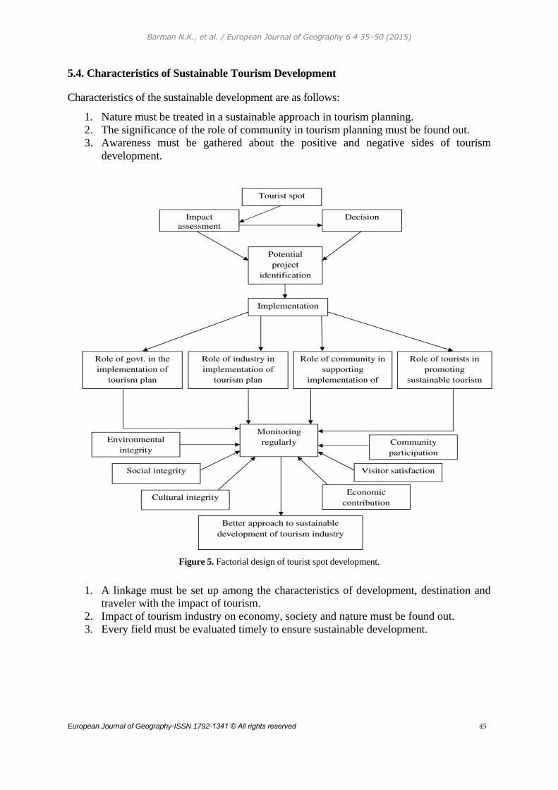
Barman N.K., et al. / European Journal of Geography 6 4 35–50 (2015)
European Journal of Geography-ISSN 1792-1341 © All rights reserved 45
5.4. Characteristics of Sustainable Tourism Development
Characteristics of the sustainable development are as follows:
1. Nature must be treated in a sustainable approach in tourism planning.
2. The significance of the role of community in tourism planning must be found out.
3. Awareness must be gathered about the positive and negative sides of tourism
development.
Figure 5. Factorial design of tourist spot development.
1. A linkage must be set up among the characteristics of development, destination and
traveler with the impact of tourism.
2. Impact of tourism industry on economy, society and nature must be found out.
3. Every field must be evaluated timely to ensure sustainable development.
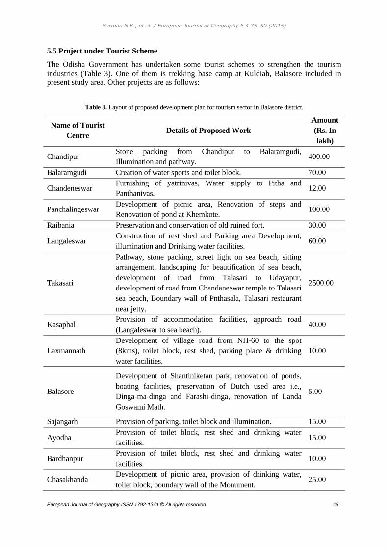
Barman N.K., et al. / European Journal of Geography 6 4 35–50 (2015)
European Journal of Geography-ISSN 1792-1341 © All rights reserved 46
5.5 Project under Tourist Scheme
The Odisha Government has undertaken some tourist schemes to strengthen the tourism
industries (Table 3). One of them is trekking base camp at Kuldiah, Balasore included in
present study area. Other projects are as follows:
Table 3. Layout of proposed development plan for tourism sector in Balasore district.
Name of Tourist
Centre Details of Proposed Work
Amount
(Rs. In
lakh)
Chandipur Stone packing from Chandipur to Balaramgudi,
Illumination and pathway. 400.00
Balaramgudi Creation of water sports and toilet block. 70.00
Chandeneswar Furnishing of yatrinivas, Water supply to Pitha and
Panthanivas. 12.00
Panchalingeswar Development of picnic area, Renovation of steps and
Renovation of pond at Khemkote. 100.00
Raibania Preservation and conservation of old ruined fort. 30.00
Langaleswar Construction of rest shed and Parking area Development,
illumination and Drinking water facilities. 60.00
Takasari
Pathway, stone packing, street light on sea beach, sitting
arrangement, landscaping for beautification of sea beach,
development of road from Talasari to Udayapur,
development of road from Chandaneswar temple to Talasari
sea beach, Boundary wall of Pnthasala, Talasari restaurant
near jetty.
2500.00
Kasaphal Provision of accommodation facilities, approach road
(Langaleswar to sea beach). 40.00
Laxmannath
Development of village road from NH-60 to the spot
(8kms), toilet block, rest shed, parking place & drinking
water facilities.
10.00
Balasore
Development of Shantiniketan park, renovation of ponds,
boating facilities, preservation of Dutch used area i.e.,
Dinga-ma-dinga and Farashi-dinga, renovation of Landa
Goswami Math.
5.00
Sajangarh Provision of parking, toilet block and illumination. 15.00
Ayodha Provision of toilet block, rest shed and drinking water
facilities. 15.00
Bardhanpur Provision of toilet block, rest shed and drinking water
facilities. 10.00
Chasakhanda Development of picnic area, provision of drinking water,
toilet block, boundary wall of the Monument. 25.00

Barman N.K., et al. / European Journal of Geography 6 4 35–50 (2015)
European Journal of Geography-ISSN 1792-1341 © All rights reserved 47
ChoumukhaDagra Provision of accommodation, illumination, road from
Kalipada to beach (8kms). 40.00
Tipisigadia Development of road (3kms) from NH-5, parking,
illumination, toilet block and drinking water facilities. 50.00
Kupari Development of toilet block, rest shed and parking area. 25.00
Inchudi Provision of toilet facilities. 5.00
Gud Rest shed and parking area development, illumination and
drinking water facilities. 25.00
Total 3482.00
Source: Comprehensive district annual plan 2011-2012 (Balasore).
5.6 Strategies for Tourism Industry Development
The beautiful natural setting, 64km long coastline exiting sand dune and the confluence of the
rivers are ideal background to develop the tourism industry.
The strategies of building up tourism industries are as follows:
Good quality road should be constructed up to all tourist spots.
Enough scope of accommodation should be arranged in all tourist spots.
Supply of electricity and drinking water should be ensured.
Trained guide and public transportation should be ensured.
All tourist spots of the present study area should be interconnected.
The State Government should pay attention to tourism industry to collect more tax.
The Government should find out new spots and develop them for the tourism.
CONCLUSION
Coastal zone, the transitional zone between land and sea, is one of the most fragile, complex
and a productive ecosystem. It is bestowed with enormous resources both - living, non-living
and is a potential area for recreation and harnessing non-conventional energy resources (wave
and wind energy). Accelerated and unscientific developmental activities have induced
catastrophic consequences. In order to optimally utilize and reap the benefits without
hampering the balance, it is necessary to adopt integrated coastal management strategies based
on solid scientific foundation that allow for multiple uses of the resources without causing
serious damage to the environment.
Coastal ecosystems found along continental margins are regions of remarkable biological
productivity and high accessibility. This has made them centers of human activity for millennia.
Coastal ecosystems provide a wide array of goods and services: they host the world’s primary
ports of commerce; they are the primary producers of fish, shellfish, and seaweed for both
human and animal consumption and they are also a considerable place of tourism industry
development. The beauty of coastal ecosystems makes them a magnet for the world’s
population. People drift down to coastal regions to live as well as for leisure, recreational
activities and tourism. For purposes of this analysis the coastal zone has been defined to include
the intertidal and sub tidal areas on and above the continental shelf (to a depth of 200 meters)
and immediately adjacent lands.
Recently Central Government has approved an ICZM (Integrated Coastal Zone
Management) project at a cost of Rs.1156 crore to build up capacity and establishment to
efficiently execute the Coastal Regulation Zone Notification (1991) aimed to control pollution
of coastal waters and to increase livelihood options for coastal communities.
Barman N.K., et al. / European Journal of Geography 6 4 35–50 (2015)
European Journal of Geography-ISSN 1792-1341 © All rights reserved 48
REFERENCES
Atkinson, G., Dubourg, R., Hamilton, K., Munasinghe, M., Pearce, D., & Young, C. (1997),
Measuring Sustainable Development: macroeconomics & the environment. Cheltenham:
Edward Elgar Publishing Limited, pp. 252.
Bbernroider, E., (2002). Factors in SWOT Analysis Applied to Micro, Small to Medium, and
Large Software Enterprises: An Austrian Study. European
Management Journal, 20(5):562573. Elsevier Science Ltd. Printed in Great Britain
Bird,E.C.F., (2000). Coastal geomorphology: an introduction. John Wiley, Chichester, UK.
Bryant,E.,(2005). Natural hazards, 2nd edition (Cambridge University Press, Cambridge).
Burston, J., (2007). Stochatic model of extreme coastal water levels, New South Wales,
Australia. PhD THESIS. University of Sydney, Australia.
Capobianco, M., de Vriend, H., Nicholls, R., Stive, M.J.F., (1999).Coastal area impact &
vulnerability assessment: the point of view of a morphodynamic modeler, Journal of
Coastal Research, 15(3),701-716
Chang, H.H., and Huang, W.C., (2006). Application of a quantification SWOT
analytical method. Mathematical and Computer Modelling, Elsevier, 43:158–169.
Clark, J.R., (1992). Integrated Management of Coastal Zones, FAO Fisheries Technical
Paper, No. 327, Food & Agriculture organization of the United Nations, Rome.
Coast Learn, (May 2009). Sustainable Tourism, Available at http://www.coastlearn.org/
Durovic, M., Lovrentjev, S., (2014). Indicators of Sustainability in Cultural Tourism, The
Macrotheme Review, A Microdisciplinary journal of global macrotrends. 3 (7),51.[39]
Dyson, R.G., (2004). Strategic development and SWOT analysis at the University of
Warwick. European Journal of Operational Research 152: 631–640. Science Direct.
Elsevier.
EEA, (2006). The changing faces of Europes Coastal areas, EEA6/2006, European
Environment Agency, Copenhagen.
Ehler, C. N., Cicin-Sain, B., Knecht, R., South, R. and Weiher, R., (1997). Guidelines to
assist policy makers and managers of coastalareas in the integration of coastal
management programmes andnational climate-change action lans, Ocean & Coastal
Management, Vol. 37, No. 1, pp. 7-27.
Gossling, S., (2003). “ Market integration and ecosystem”
Harris, L.D., (1963). Characteristics of the Hurricane storm surge U.S. Weather Bureau,
Technical paper No. 48
Hart, M., (1999). Guide to Sustainable Community Indicators. North Andover, MA: Hart
Environmental Data.
Houben, G., Lenie K., and Vanhoof, K., (1999). A knowledge based SWOT analysis
system as an instrument for strategic planning in small and medium sized enterprises.
Decision Support Systems, Elsevier, 26:125–135.
Barman N.K., et al. / European Journal of Geography 6 4 35–50 (2015)
European Journal of Geography-ISSN 1792-1341 © All rights reserved 49
IESWM, (2010). Environmental Impact Assessment & Social Impact Assessment, Under
National Cyclone Risk Mitigation Project of North 24 Pargana District, W.B. Institute of
Environmental Studies & Wetland Management, Kolkata.
Inskeep, E., (1991). Tourism Planning: An Integrated &Sustainable Development Approach,
John Wiley & Sons, Toronto.
Jensen, K., (1998). Environmental Impact Assessment Using the Rapid Impact
Assessment Matrix (RIAM). Olsen & Olsen (Publisher), Fredensborg, Denmark, pp. 69.
Kaiser, G., (2006). Risk & vulnerability analysis to coastal hazards-an approach to
integrated assessment, PhD thesis, Christian Albrecht University, Kiel, Germany.
Kanji, F., (2006). A global perspective on the challenges of coastal tourism, Coastal
Development Centre, Bangkok.
Leatherman, S.P., Zhang, K., and Douglas, B.C, (2000). Sea levelrise shown to drive coastal
erosion. EOS, Transactions of the American Geophysical Union. 81(6), 55-57.
Making Tourism More Sustainable - A Guide for Policy Makers, UNEP and UNWTO,
(2005), p.11-12.
McLaren,D., (2003). Rethinking tourism and ecotravel. Second Ed. CT: Kumarian Press, Inc.
Miller. M., Auyong, J, and Hadley, N.P., (eds) (2002). Sustainable Coastal Tourism:
Challenges for Management, Planning &Education, in: Proceedings of the 1999
International Symposium on Coastal & Marine Tourism: Balancing Tourism &
Conservation, University of Washington, Oregon State University& Oceans
Blue Foundation, Seattle, W.A, pp. 3-20.[88]
Morris, P., and Biggs, J., (1995). Water. In: P. Morris and R. Therivel (eds), Methods of
Environmental Assessment, UCL Press, UK.
Moseley, M. J., (2002). Sustainable rural development: The role of community involvement
& local partnership. NATO Advanced Research Workshop. Krakow, Poland, Nov.2002.
Neto,F., (2003). “ A new approach to sustainable tourismdevelopment: Moving beyond
environmental protection”. Natural Resources Forum, No.27,3,PP.212-222.
Nott, J., and Hayne, M., (2000). How high was the storm surge from tropical cyclone
Mahina, North Queensland, 1999. Aust J.Emer. Mgmt. 15, 11-13.
Nouri, J., Karbassi, A.R., and Mirkia, S., (2008). Environmental management of coastal
regions in the Caspian Sea. Int. J. Environ. Sci. Tech., 5(1): 4352.
Pastakia, C.M.R., (1998). The Rapid Impact Assessment Matrix (RIAM) – A New Tool for
Environmental Impact Assessment. In: Kurt Jensen (ed.), Environmental Impact
Assessment Using the Rapid Impact Assessment Matrix (RIAM), Olsen & Olsen,
Fredensborg, Denmark.
Paul, A.K., (2002). Coastal Geography & Environment : Sundarban Coastal Plain, Kanthi
Coastal Plain & Subarnarekha Delta Plain, ACB Publications, Kolkata, pp. 575.
Sadler, B., (2004). On evaluating the success of EIA &SEA. Assessing Impact: Handbook of
EIA & SEA follow-up, Morrison-Saunders A & Arts J, London, Earth scan, pp. 248-285.
Barman N.K., et al. / European Journal of Geography 6 4 35–50 (2015)
European Journal of Geography-ISSN 1792-1341 © All rights reserved 50
Sanò, M., and Fierro, G., (2003). Integration of the SWOT analysis as a coastal
management tool with a geographical information system: Two approaches to the
problem and first results Dipartimento per lo studio del Territorio e delle sue Risorse
(Dip.Te.Ris.) Università di Genova (IT), University of Georgia.
Sommez, S.F., and Graefe, A.R., (1998), Determining future travel behaviour from past
travele xperience and perceptions of risk and safety. Journal of Travel Research, 37, pp.
171-177.
Sorensen, J., (1993). The International Proliferation of Integrated Coastal Zone Management
Efforts. Ocean and Coastal management, No, 21, PP. 45-80.
TERI, (2011). Measuring, monitoring & managing sustainability in Indian coastal areas: The
socio economic dimensions.
UNEP, (2009). Sustainable Coastal Tourism : An integrated planning & management
approach.
UNWTO, (1994). National & Regional Tourism Planning: Methodologies & Case Studies,
WTO, Madrid.
Wong, P.P., (1993). Tourism versus Environment: the case forcoastal areas. Boston. Kluwer
Publisher, Dordrecht.
European Journal of Geography Volume 6, Number 4: 51-58, December 2015
©Association of European Geographers
European Journal of Geography-ISSN 1792-1341 © All rights reserved 51
IDENTIFICATION OF WEAKNESSES AND STRENGTHS OF TOURISM
DEVELOPMENT IN KANDOLEH VILLAGE, IRAN.
Aeizh AZMI Razi University, Department of Geography, Kermanshah, Iran
Akram RAZLANSARI Razi University, Department of Geography, Kermanshah, Iran
Abstract
This study aims to identify strengths and weaknesses and provide strategies for tourism
development in Kandoleh village. Investigative method was descriptive and we used from
SWOT model to analyze data. At first, using field studies and documents and using thematic
experts, a list of weaknesses, strengths, opportunities and threats of rural tourism was
prepared. Then, the list in the form of Likert scale questionnaire was designed and we have
distributed questionnaires among tourists in kandoleh village. Then, the internal and external
factors in the development of rural tourism were analyzed. The results showed that the
average for total internal strengths 4.12 and its total weight is 2.16, but the average for total
internal weakness 3.51 and its total weight is 1.74. This shows that rural tourism’s strengths
outweigh the weaknesses. The average for strength was 3.56 and its total weight is 1.81. The
average for threats 2.88 and its total weight is 1.41. In general, higher the weight of the
strengths and opportunities revealed that best strategies for tourism development include the
following: Attention on the development of tourism due to the natural green landscape,
gardens and good climate, increased government attention to tourism, identification and use
of resources according to the specific situation of village, creation incentives to compete with
other regions for tourism development, development and strengthening of roads.
Keywords: tourism development, strengths and weaknesses, Kandoleh village, Iran country, SWOT
model
1. INTRODUCTION
In today's world, rural tourism as a strategy for rural development is used and many thinkers
and planners have special attention to it, because they believe that the development of rural
tourism is one of the suitable strategies for rural development and it solves challenges and
problems.
Rural tourism is one of the forms of tourism that can lead to economic growth and
diversification of the activities and the creation of employment and income for rural residents
to absorb the surplus manpower. So rural tourism is profit for rural development (Papoli Yazi
& Saghaei, 2011, p201). The village economy is based on agriculture and therefore
vulnerable. So attention to other activities such as tourism helps to the rural economy and to
improve the living conditions of rural people. Rural tourism in empowerment of local people
and develop human resources, improve living standards and bridge the gap between urban
Azmi A. & Razlansari A. / European Journal of Geography 6 4 51–58 (2015)
European Journal of Geography-ISSN 1792-1341 © All rights reserved 52
and rural areas in various fields and to reduce rural-urban migration has played an important
role(Mahdavi, Ghadiri Maasoum & Ghahremani,2008,p43). Supporters and opponents
believe that rural tourism makes up the rural economy, improve the viability of rural areas,
settlements reconstruction and improve the lives of rural communities (Eftekhari & Mahdavi,
2006, p2).
Rural tourism is important in two aspects: one as a global activity and the role of the
national development. In this regard, rural tourism is an ultra structural function and can
develop participation with rural people. It has relationship with economic and cultural sectors
in village and contributes to national development (Shameddin, 2010, pp96-97). Rural
tourism provides new opportunities for the rural areas due to the stability of rural settlements,
but on the other hand it needs to guide development and planning and to solve social and
environmental problems (Darvishi et al.,2014,pp70-71). Thus, several studies have been
conducted about the effects of tourism on the countryside.
Darvishi and et al (2014) using the SWOT model to prioritize strategies for rural tourism
development in the village Gaygan Aligoudarz city. They suggest those aggressive strategies
such as education and physical, social and spatial planning of villages, creating mechanisms
for investment in government and the private sector is suitable for tourism development.
Karimi and Sharifi (2013) research in the County of Maragheh and found that the strength
point is natural attractions and weakness points are lack of accommodation, welfare, health
and sport.Khaton Abadi and Rast Ghalam(2012) using SWOT model concluded that the
limitations of tourism are at a higher level than its advantages.Eftekhari and et al (2006)
studied strategies in rural Lavasan districts and their findings indicate that the vulnerability of
rural areas in terms of tourism development is often very high and preferences in mainly rural
areas are limited.
In general, local characteristics, customs, traditional, natural and historical attractions in
rural areas has led to the development of tourism. Kermanshah Province is a province that
many people go there for tourism. So many people go for leisure and recreation to
Kermanshah province. Kandoleh village is located in Kermanshah province is tourism
village. Regarding the issue of tourism development in the village and identify the
advantages, benefits, problems and injuries is important. The main objective of this study is
to identify the strengths and weaknesses of rural tourism of Kandoleh village and provide
strategies for tourism development in the village. Through identifying the potential and
limitations of tourism in this region is improved planning and solving problems. So the main
question of this research is that what is Strengths, weaknesses, opportunities and threats
facing the tourism village Kandoleh?
2. MATERIALS AND METHOD
This research is descriptive and SWOT method was used to analyze the data. At first, using
field studies and documents, and the use of subject experts, a list of weaknesses, strengths,
opportunities and threats of village tourism Kandoleh developed (Table 1). Then, a
questionnaire with Likert scale was designed and distributed among visitors. Then the
internal and external factors tourism development of Kandoleh village was analyzed and
priorities were identified.
In order to define strengths, weaknesses, opportunities and threats SWOT model can be used
the following simple words:
Strengths: characteristics that assist the group in achieving objectives. These properties have
a positive effect on their goals;
Weaknesses: attributes that are harmful and negative impact to achieve their goals;

Azmi A. & Razlansari A. / European Journal of Geography 6 4 51–58 (2015)
European Journal of Geography-ISSN 1792-1341 © All rights reserved 53
Opportunities: the condition of the environment which could be due to the positive effects
that may assist the group in achieving goals;
Threats: condition of the environment in the way of achieving the objectives are created limit
(Azkia & et al., 2008, pp143-144).
Table 1. List the strengths, weaknesses, opportunities, threats tourism village of Kandoleh
Strengths Having adequate facilities and equipment such as water, electricity, gas and
telephone;
Religious and historical monuments near the village;
Locating near population centers;
Natural landscapes, orchards and vineyards;
Variety of agricultural products;
Crafts and local foods;
River in the vicinity of the village tourism facilities, such as the ability to provide
health services;
Local authorities pay special attention to the development of rural tourism;
good climate in some months of the year;
The spirit of hospitality in the village.
Weaknesses The lack of residential facilities in the village;
The low quality of local health (lack of sewage and waste release);
Lack of local markets for sale of agricultural products, local handicrafts to
tourists;
Lack of health care in rural areas;
Migration of rural residents to cities around;
The lack of investment for the private sector to provide services to tourists;
The lack of accurate data on the number of tourists to better planning;
Insufficient information and advertising in order to introduce a better system of
village and tourist attraction;
Lack of knowledge of villagers on how to deal and interact with tourists.
Opportunities Public sector investment for residential welfare services;
The possibility of attracting non-local investment and the private sector;
Good roads to facilitate the movement of tourists;
Planning and continuous monitoring of public organizations to implement
security programs in rural tourism;
Providing new economic opportunities for rural residents;
Restore jobs and local industries obsolete in the village;
To create a positive attitude of people regarding the development of tourism;
Increase the efficiency of agricultural products;
Finding a special position for the village in the County.
Threats Environmental pollution by increasing the number of tourists;
The loss of plant and animal species by increasing the number of tourists;
The loss of local traditions due to an increase in the number of tourists;
The lack of a clear understanding of rural tourism among tourists;
Lack of investment in different sectors of the economy due to the fear of failure;
Crime increase with the entrance of non-native to the village;
A lack of understanding of the potential of regions among managers;
The lack of the necessary cooperation between organizations involved in rural
development;
Changing in attitude of rural youth by increasing the number of tourists
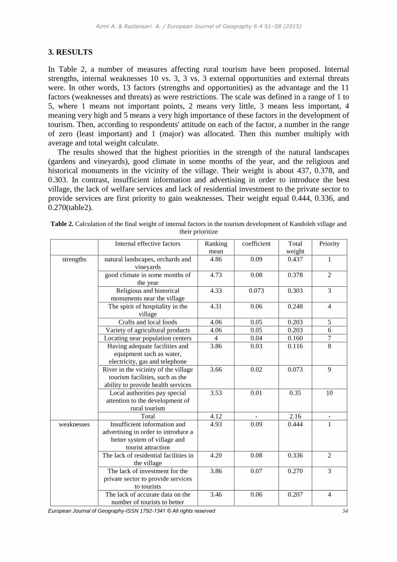
Azmi A. & Razlansari A. / European Journal of Geography 6 4 51–58 (2015)
European Journal of Geography-ISSN 1792-1341 © All rights reserved 54
3. RESULTS
In Table 2, a number of measures affecting rural tourism have been proposed. Internal
strengths, internal weaknesses 10 vs. 3, 3 vs. 3 external opportunities and external threats
were. In other words, 13 factors (strengths and opportunities) as the advantage and the 11
factors (weaknesses and threats) as were restrictions. The scale was defined in a range of 1 to
5, where 1 means not important points, 2 means very little, 3 means less important, 4
meaning very high and 5 means a very high importance of these factors in the development of
tourism. Then, according to respondents' attitude on each of the factor, a number in the range
of zero (least important) and 1 (major) was allocated. Then this number multiply with
average and total weight calculate.
The results showed that the highest priorities in the strength of the natural landscapes
(gardens and vineyards), good climate in some months of the year, and the religious and
historical monuments in the vicinity of the village. Their weight is about 437, 0.378, and
0.303. In contrast, insufficient information and advertising in order to introduce the best
village, the lack of welfare services and lack of residential investment to the private sector to
provide services are first priority to gain weaknesses. Their weight equal 0.444, 0.336, and
0.270(table2).
Table 2. Calculation of the final weight of internal factors in the tourism development of Kandoleh village and
their prioritize
Internal effective factors Ranking
mean
coefficient Total
weight
Priority
strengths natural landscapes, orchards and
vineyards
4.86 0.09 0.437 1
good climate in some months of
the year
4.73 0.08 0.378 2
Religious and historical
monuments near the village
4.33 0.073 0.303 3
The spirit of hospitality in the
village
4.31 0.06 0.248 4
Crafts and local foods 4.06 0.05 0.203 5
Variety of agricultural products 4.06 0.05 0.203 6
Locating near population centers 4 0.04 0.160 7
Having adequate facilities and
equipment such as water,
electricity, gas and telephone
3.86 0.03 0.116 8
River in the vicinity of the village
tourism facilities, such as the
ability to provide health services
3.66 0.02 0.073 9
Local authorities pay special
attention to the development of
rural tourism
3.53 0.01 0.35 10
Total 4.12 - 2.16 -
weaknesses
Insufficient information and
advertising in order to introduce a
better system of village and
tourist attraction
4.93 0.09 0.444 1
The lack of residential facilities in
the village
4.20 0.08 0.336 2
The lack of investment for the
private sector to provide services
to tourists
3.86 0.07 0.270 3
The lack of accurate data on the
number of tourists to better
3.46 0.06 0.207 4
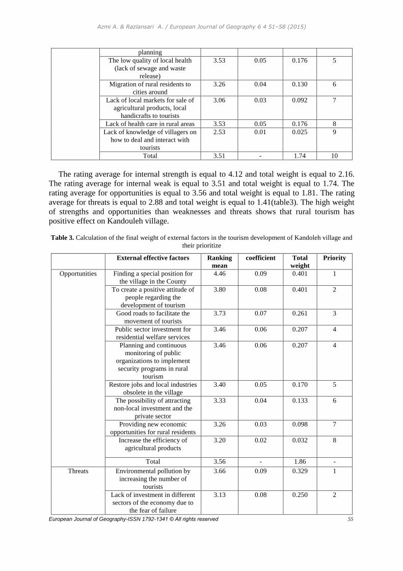
Azmi A. & Razlansari A. / European Journal of Geography 6 4 51–58 (2015)
European Journal of Geography-ISSN 1792-1341 © All rights reserved 55
planning
The low quality of local health
(lack of sewage and waste
release)
3.53 0.05 0.176 5
Migration of rural residents to
cities around
3.26 0.04 0.130 6
Lack of local markets for sale of
agricultural products, local
handicrafts to tourists
3.06 0.03 0.092 7
Lack of health care in rural areas 3.53 0.05 0.176 8
Lack of knowledge of villagers on
how to deal and interact with
tourists
2.53 0.01 0.025 9
Total 3.51 - 1.74 10
The rating average for internal strength is equal to 4.12 and total weight is equal to 2.16.
The rating average for internal weak is equal to 3.51 and total weight is equal to 1.74. The
rating average for opportunities is equal to 3.56 and total weight is equal to 1.81. The rating
average for threats is equal to 2.88 and total weight is equal to 1.41(table3). The high weight
of strengths and opportunities than weaknesses and threats shows that rural tourism has
positive effect on Kandouleh village.
Table 3. Calculation of the final weight of external factors in the tourism development of Kandoleh village and
their prioritize
External effective factors Ranking
mean
coefficient Total
weight
Priority
Opportunities Finding a special position for
the village in the County
4.46 0.09 0.401 1
To create a positive attitude of
people regarding the
development of tourism
3.80 0.08 0.401 2
Good roads to facilitate the
movement of tourists
3.73 0.07 0.261 3
Public sector investment for
residential welfare services
3.46 0.06 0.207 4
Planning and continuous
monitoring of public
organizations to implement
security programs in rural
tourism
3.46 0.06 0.207 4
Restore jobs and local industries
obsolete in the village
3.40 0.05 0.170 5
The possibility of attracting
non-local investment and the
private sector
3.33 0.04 0.133 6
Providing new economic
opportunities for rural residents
3.26 0.03 0.098 7
Increase the efficiency of
agricultural products
3.20 0.02 0.032 8
Total 3.56 - 1.86 -
Threats Environmental pollution by
increasing the number of
tourists
3.66 0.09 0.329 1
Lack of investment in different
sectors of the economy due to
the fear of failure
3.13 0.08 0.250 2
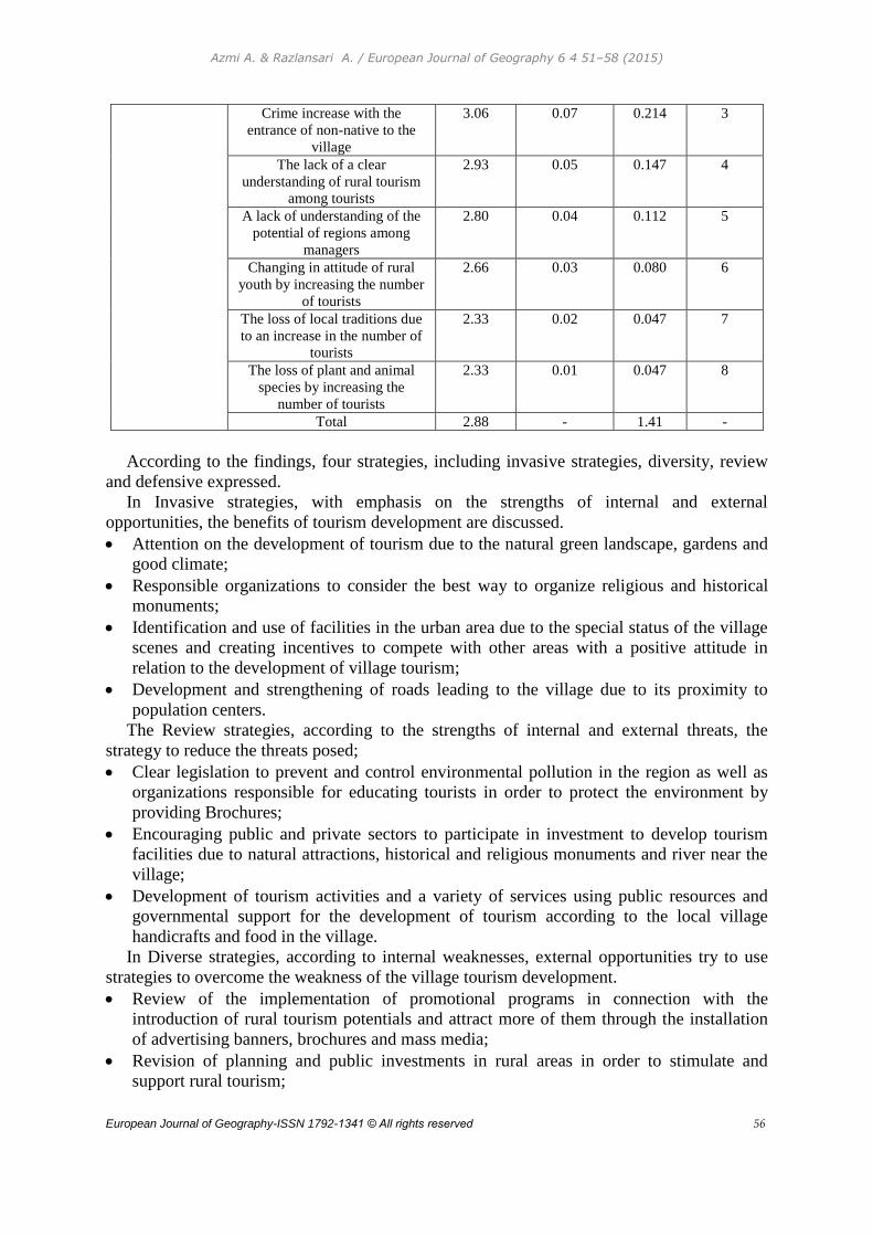
Azmi A. & Razlansari A. / European Journal of Geography 6 4 51–58 (2015)
European Journal of Geography-ISSN 1792-1341 © All rights reserved 56
Crime increase with the
entrance of non-native to the
village
3.06 0.07 0.214 3
The lack of a clear
understanding of rural tourism
among tourists
2.93 0.05 0.147 4
A lack of understanding of the
potential of regions among
managers
2.80 0.04 0.112 5
Changing in attitude of rural
youth by increasing the number
of tourists
2.66 0.03 0.080 6
The loss of local traditions due
to an increase in the number of
tourists
2.33 0.02 0.047 7
The loss of plant and animal
species by increasing the
number of tourists
2.33 0.01 0.047 8
Total 2.88 - 1.41 -
According to the findings, four strategies, including invasive strategies, diversity, review
and defensive expressed.
In Invasive strategies, with emphasis on the strengths of internal and external
opportunities, the benefits of tourism development are discussed.
Attention on the development of tourism due to the natural green landscape, gardens and
good climate;
Responsible organizations to consider the best way to organize religious and historical
monuments;
Identification and use of facilities in the urban area due to the special status of the village
scenes and creating incentives to compete with other areas with a positive attitude in
relation to the development of village tourism;
Development and strengthening of roads leading to the village due to its proximity to
population centers.
The Review strategies, according to the strengths of internal and external threats, the
strategy to reduce the threats posed;
Clear legislation to prevent and control environmental pollution in the region as well as
organizations responsible for educating tourists in order to protect the environment by
providing Brochures;
Encouraging public and private sectors to participate in investment to develop tourism
facilities due to natural attractions, historical and religious monuments and river near the
village;
Development of tourism activities and a variety of services using public resources and
governmental support for the development of tourism according to the local village
handicrafts and food in the village.
In Diverse strategies, according to internal weaknesses, external opportunities try to use
strategies to overcome the weakness of the village tourism development.
Review of the implementation of promotional programs in connection with the
introduction of rural tourism potentials and attract more of them through the installation
of advertising banners, brochures and mass media;
Revision of planning and public investments in rural areas in order to stimulate and
support rural tourism;
Azmi A. & Razlansari A. / European Journal of Geography 6 4 51–58 (2015)
European Journal of Geography-ISSN 1792-1341 © All rights reserved 57
Re-governmental organizations in the utilization of public participation for the intended
use of the benefits and advantages tourism.
In Defensive strategies strategy, with emphasis on reducing vulnerabilities and threats,
solutions are offered.
Open concept of rural tourism among tourists, as well as educating villagers about better
interaction with tourists;
Residential development in the village with the participation of the private sector and
public utilities and attract investments;
Cultural Heritage and Tourism institute planning for balanced development of rural
tourism, as well as to identify the facilities and capabilities of the villages;
Exhibition of crafts and local foods in the village in order to identify customs.
4. CONCLUSIONS
Rural tourism contributes to economic growth and diversification of activities in the village.
Agricultural activity is vulnerable to natural hazards; therefore the development of other
activities such as rural tourism should be a fundamental subject. This leads to better rural
livelihoods and reduce migration.
The tourism seems to be the sector as a supplement to the income of rural people. Studies
and the results showed that domestic factors are the highest priority on the strengths of the
components of natural landscapes, gardens. Studies showed that the highest priority on the
strengths is the components of natural landscapes, garden. Its weight was 0.437. The first
priority of the weaknesses was the poor system of information and advertising for attract
tourism. Its weight was 0.444. The first priority of the opportunities was special status of the
village in the county. Its weight was 0.401. The first priority of the threats was environmental
pollution by increasing the number of tourists. Its weight was 0.329.
Generally, the higher the weight of strengths and opportunities against weaknesses and
threats indicate that the best strategies to develop rural tourism are invasive strategies. These
strategies include: attention on the development of tourism due to the natural green
landscape, gardens and good climate; responsible organizations to consider how best to
organize religious and historical monuments; identification and use of facilities in the urban
area due to the special status of the village scenes and creating incentives to compete with
other areas with a positive attitude in relation to the development of village tourism;
development and strengthening of roads leading to the village due to its proximity to
population centers.
In the end, the following is recommended to improve the development of tourism in the
Kandoleh village:
Preserve natural landscapes and lush countryside and the environment in cooperation
with state and public participation;
Develop and implement plans and principles for the development and diversification
of rural tourism development, marketing and advertising programs;
Development of services and facilities needed due to the position of rural tourism in
the county, with the support of the government and the private sector with the aim of
improving the quality of rural tourism.
Meetings by tourism authorities to increase the level of awareness of people about the
advantages of rural tourism.
Azmi A. & Razlansari A. / European Journal of Geography 6 4 51–58 (2015)
European Journal of Geography-ISSN 1792-1341 © All rights reserved 58
REFERENCES
Armed Forces Geographical Organization.1995, Geographical encyclopedia of Kermanshah
province, Iran, Tehran, Armed Forces Geographical Organization Press, 767 pages.
Azkia. Mostafa, Zare. Adel, Imani.Ali.2008, Approach and qualitative research methods in
rural development, Iran,Tehran, Nei press, 300 pages.
Darvishi. Hedayatoollah, Beiranvand Zadeh. Maryam, Dehghani Alvar. Seyyed Ali Nader,
Ahmadi. Sajjad .2014, Prioritization of tourism development strategies in terms of land
use-case study: Gaigan village, Aligodarz county, Rural Development Strategy Journal,
vol. 1, no2, pp69-84.
Karami. Fariba, Sharifi. Fahimeh.2013, Evaluation of rural tourism by using SWOT-Case
study, villages of Maragheh county, Geography and planning journal, year 17, no46,
pp173-196.
Kermanshah province, Detailed results of the General Census of Population and Housing
of.2011, available at http://www.ostan-ks.ir
Khatoon Abadi. Rast Ghalam.Mehdi.2011, Assessment of the four pillars of rural tourism
with SWOT-case study: villages of Cheharmahal and Bakhtiari province, Economic and
Tourism Development Journal, vol.25, no3, pp330-338.
Mahdavi. Masoud, Ghadiri Maasoum. Mojtaba, Ghahremani. Nasrin.2008, The effects of
tourism on the development of rural tourism with survey of the villagers in Kan and
Sooleghan valley, Village and development journal, year 11, no 2,pp39-60.
Papoli Yazdi. Mohammad Hosein, Saghaei. Mahdi.2011, tourism(principles and concepts),
Iran, Tehran, Samt Press, 275 pages.
Rokn Edin Eftekhari. Abdolreza, Mahdavi. Davood.2006, Rural tourism development
strategies using the SWOT model-case study: Lavasan district, Education Humanity
Science Journal, no45, pp1-30.
Shamseddini. Ali.2010, Rural tourism, productive strategies for rural development, House
and Rural Environment Journal, no131, pp95-107.
European Journal of Geography Volume 6, Number 4: 59- 75, December 2015
©Association of European Geographers
European Journal of Geography-ISSN 1792-1341 © All rights reserved 59
SCENARIO-BASED LOCATION OF AMBULANCES FOR SPATIOTEMPORAL
CLUSTERS OF EVENTS AND STOCHASTIC VEHICLE AVAILABILITY. A
DECISION SUPPORT SYSTEMS APPROACH.
Yorgos N. PHOTIS
Department of Geography and Regional Planning, National Technical University of Athens, Greece
Stavros A. SIRIGOS
Department of Planning and Regional Development, University of Thessaly, Volos, Greece
Abstract
Facility location through the utilization of location-allocation models is a scientific field that
has been rapidly growing over the last 60 years. Especially in countries where there is an
increased need for new infrastructure and services while resources and funding availability is
limited, their application in solving respective problems can be effective both in catalyzing
needs as well as minimizing required budget and costs. In this context, new models,
improved algorithms and alternative methodological approaches have been constantly arising.
In Greece, unfortunately, the use of these models is not a common practice in locational
projects and studies resulting in relatively limited corresponding experience and research. In
this paper we present S-Distance, a stand alone locational analysis and planning support
system, initially designed at the Laboratory for Spatial Analysis, GIS and Thematic
Cartography in the University of Thessaly, Greece and currently under further development
by the GeoCHOROS Geospatial Analysis and GIS Research Group at the National Technical
University of Athens, Greece. The operational validity of the proposed system was verified
for the location of ambulances in the metropolitan area of Volos and Nea Ionia in Greece.
Keywords: location-allocation, Spatial Decision Support System, optimization algorithms, EMS
1. INTRODUCTION
Location planning of a service delivery network is undoubtedly a complicated task. This is
mainly due to the fact that the location of service centers and facilities, both in the public and
private sector, is tied to decisions relevant to the number of units in the area as well as their
characteristics,. These decisions are interrelated and interdependent and thus, spatial, social,
political, economic and individual data should be combined and co-examined.
Research in recent years has shown that, contrary to what was assumed until now,
especially for densely populated areas, the environment within which location decisions are
taken is characterized by uncertainties (Snyder, 2006). Thus, for example, uncertainties have
been identified concerning the demand which supply centers have to cover as well as
uncertainties related to the transportation network impedance, whether it refers to travel time
or cost. At the same time, and given the extensive investment in resources and infrastructures,
locational planning policies and decisions are expected to last for a significant period of time.
Photis N.Y. & Syrigos A. S. / European Journal of Geography 6 4 59–75 (2015)
European Journal of Geography-ISSN 1792-1341 © All rights reserved 60
Therefore, certain predefined problem parameters, which are not defined with certainty
during the decision-making process, should be handled as uncertain or random. In this
respect, addressing this issue requires a location analysis model, which takes into account the
inevitable uncertainty of decisions over time. (Sirigos, 2004).
Aiming to address the growing complexity of locational planning, research, during the last
thirty years, has moved towards the design and development of geospatial information
systems which will support the relating decision-making process. Such information systems
compile and combine methods and techniques from the scientific areas of geoinformation,
location theory, regional development and geospatial analysis.
In this paper we present S-Distance, a stand alone locational analysis and planning support
system, initially designed at the Laboratory for Spatial Analysis, GIS and Thematic
Cartography in the University of Thessaly and currently distributed by the GeoCHOROS
Geospatial Analysis and GIS Research Group at the National Technical University of Athens,
Greece. The operational validity of the proposed system is verified through the location of
ambulances in the metropolitan area of Volos and Nea Ionia in Greece; the location-
allocation model that was formulated, optimizes response for the worst case scenario, taking
into account the stochastic nature as well as the hierarchical structure of the problem, when
considered at the regional or country level. Alternative scenarios are generated based on the
expected geographical and temporal distribution of the emergency incidents (demand), the
traffic flow variability, the number of available ambulances (supply) as well as the
probability of an ambulance being occupied on the time of call.
2. LOCATIONAL ANALYSIS AND PLANNING
Locational analysis and / or planning refers to capturing, modeling, formulating and solving a
broad category of problems, which may be best described as siting facility operations and
activities in a given area and assigning demand to them in order to build a robust service
network. In essence, it constitutes the art and science of mathematically putting things where
they should be. The expressions deployment, positioning, and siting are frequently used as
synonyms (ReVelle and Eiselt, 2005). In its simplest form, a “services network” is regarded
to be a set of generally similar service centres, which are required to meet a certain demand.
To this end, locational planning problems deal with the spatial organization of services,
which respectively require the location of centres and the allocation of demand to them,
according to specific constraints. A typical location problem is mainly defined by four (4)
decision variables: a) the spatial distribution of demand, which is usually located in points
(nodes) or paths, b) the nature and the characteristics of the service network, c) the area in
which demand has to be allocated and service centres located and d) the metric which denotes
(time) distances or the service cost of demand with respect to the locations of the feasible
sites (candidate locations) on the study network which is usually reflected to a distance
matrix.
2.1. Location - allocation models
Numerous factors play an important role in the modeling of location problems, apart from the
basic parameters described above. Such a factor is the objective, which according to the
nature of the problem is set by the decision-makers and has to be either minimized or
maximized. In several cases, such as ambulance location problems, the primary target is for
supply locations to be or get as close as possible to demand. On the contrary, when selecting
Photis N.Y. & Syrigos A. S. / European Journal of Geography 6 4 59–75 (2015)
European Journal of Geography-ISSN 1792-1341 © All rights reserved 61
areas for the location of radioactive waste landfills, geologically stable regions are sought,
which will be as far away as possible from densely populated areas.
In their general form, location-allocation models confront the following problem: given
the spatial distribution of demand, facilities or service centres must be located and allocation
regions must be defined around them in “the best possible way” (Photis, 2014). The “best
possible way” is achieved through the optimization of an objective function, according to
which profit is maximized or loss minimized depending on the alternative solution
configuration. The mathematical foundations of location-allocation problems were set by
Pierre de Fermat (1601-1655) and were first applied by Weber (1909) for the definition of a
point in the plane that minimizes the sum of the transportation costs from it to n destination
points, where different destination points are associated with different costs per unit distance.
2.1.1. Static models
Clinical and statistical data show that if the human brain is deprived of oxygen for more than
six minutes, then the probability of survival and continuance of a normal life is less than
50%. Thus, the locational planning process could focus on the minimization of the number of
ambulances required, so that all nodes which potentially might represent demand (e.g.
residential areas) are within a specific time distance (i.e. six minutes) from the nearest facility
or service center (ambulance). This distance is called “covering distance” and the respective
location – allocation model formulation is the “set covering”. Respectively, a demand node is
considered “covered” when the nearest service center – an ambulance in our example – is
located within a distance equal to the covering distance (analogous to the nature of the
service). Set covering models have been widely used by a number of authors and researchers
for emergency management service and response problems (Photis, 2004).
One of the most common problems associated with the set-covering model is that the
solution it proposes, locates more vehicles than the organization’s budget can afford (Daskin,
1995). Specifically, the last ambulances contribute little to the percentage of the demand’s
coverage served within the coverage distance, while they increase the service’s provision cost
significantly. This fact leads to an alternative target: the maximization of the demand served
within a given coverage distance by using a certain number of ambulances. This formulation
is known as “maximal covering model” (Church and ReVelle, 1974). In practice, the size of
the current fleet this model takes for granted ranges from 1 to the number required for the full
coverage according to the suggestion of the set covering model.
Sometimes, the determination of a given covering distance in advance is difficult and
sometimes is quite inappropriate. For example, in the examined case of ambulances, the 4-
minute covering distance may well be not the appropriate one. A shorter timeline could be
substantiated when observing that the countdown for the patient begins with the start of the
(serious) medical incident, while the reaction time counts only after the vehicle leaves its
base. A considerable time period (several minutes) very often mediates between the medical
incident and the activation of the vehicle which will move towards the expected area. This
additional time is consumed by the time of the incident’s assignment to a vehicle and
information of the crew. On the other hand, further reduction of the covering distance may be
impossible due to economical reasons. It would cost much less, instead, if the timeline was 5
minutes or more. In this way, another model is determined: the minimization of the covering
distance of the total demand, by using a given number of ambulances (i.e. minimization of
the maximum distance). Thus, the set covering’s distance is determined endogenously by the
model itself (Daskin, 1995). The above formulation is known as the “P-center model”.
The coverage and center models focus on the systems behavior in the worst case, such is
the maximum reaction time, for instance. Moreover, the view that the level of service
Photis N.Y. & Syrigos A. S. / European Journal of Geography 6 4 59–75 (2015)
European Journal of Geography-ISSN 1792-1341 © All rights reserved 62
gradually decreases, while the distance increases, is much more realistic. This observation
leads to the fourth basic model with the following formulation: the average time of response
(time between points of demand and nearest ambulance) for a given number (P) of vehicles.
This model, which is the most classic, is known as “P-median” (Daskin, 1995).
2.1.2. Dynamic and stochastic models
Static models, which were described above, ignore the stochastic (random) nature of demand
and the fact that the nearest vehicle may not be available at the time of the call. If the model’s
data get characterized as random variables, then results will be random variables as well. In
this sense, interest is focused not only on the determination of the average response time (as
in P-median model), but also on the function of demand nodes’ distribution. Moreover,
demand is as stochastic as travel times are.
Additionally, static models ignore temporal differentiation in the total intensity of calls
and the temporal differentiation in the spatial distribution of them. Temporal differentiation
of demand implies that use of fixed points may not be optimal; on the contrary, use of mobile
(continuously located) ambulances is preferred (Photis, 2004).
Unlike static models, in the dynamic ones ambulance location is examined over time. This
means that variable values may be differentiated for each period of time, but in a fixed or
predictable way. The object is the optimal service of demand for the total of the examined
timelines. On the other hand, in stochastic models, some of the variables are considered to be
uncertain. The values they receive are either connected with a possibility distribution
function, or are considered to be accidental, or are represented by a set of possible scenarios.
In this way, more characteristics which compose the real problem of location are embodied,
while the system’s behavior is examined according to variety of non-clearly defined
parameters. The main disadvantage of dynamic and stochastic models is that their solving
procedure is much more demanding than the one of the static models, while in some of them,
due to the nature or/and the number of the variables that compose the uncertainty are
practically non-solvable (Grekousis & Photis, 2014).
The issue of service centers’ availability (usually vehicles for dealing emergency
incidents) has been the subject of many articles in the relevant literature (Photis &
Grekousis, 2012). Daskin (1982 and 1983) extends the maximal covering model so as to take
into account the probability that service centers (ambulances in this case) are occupied when
demand occurs. In the model of expected maximal covering that results an expected number
of service centers is located, in order for the expected demand coverage to be maximized by
an available center. In this model, the fact that a center may be occupied is equally possible
for all service centers and independent of the existence of already occupied centers. The
model of expected maximal covering sets certain restrictions, which many researchers have
tried to loosen. For instance, Batta et al. (1989) use results from the “queuing theory” in order
to achieve a more realistic representation of reality. The models which occur accept the fact
that the probability of a center being occupied depends on the probability of another center
being occupied too (hence it may have different values). So the interaction between centers
that cover common nodes is modeled more accurately. Nevertheless, the models which are
obtained are much more difficult to be solved by the expected maximal covering model
(Owen and Daskin, 1998).
Photis N.Y. & Syrigos A. S. / European Journal of Geography 6 4 59–75 (2015)
European Journal of Geography-ISSN 1792-1341 © All rights reserved 63
3. LOCATION ANALYSIS AND PLANNING SUPPORT SYSTEMS
In a highly competitive era, both at international, EU and regional level, location planning
cannot be thought of without the necessary methodological and technological tools, which
will allow not only the current situation’s analysis (quantitatively and qualitatively), but also
the production and evaluation of high quality alternative scenarios which will improve the
current situation. Besides, the continuous development of computer systems’ capabilities and
the development of even more powerful and elaborate analysis techniques allow models
which were thought to be intractable, be treated successfully.
The international literature on location-allocation models (and general on location
analysis) is incredibly rich. However, that knowledge is not concentrated in an integrated
system which will help decision-makers in solving location problems. Thus, each researcher
has to develop himself the special tools he needs or turn to other, less appropriate, methods
and techniques. We hope that this void is going to be filled in by the creation of the S-
Distance location analysis and planning system, which has been developed since 2001 at the
Laboratory of Spatial Analysis, GIS and Thematic Mapping of the Planning and Regional
Development, Faculty of Engineering, University of Thessaly (Sirigos, 2003).
3.1 The S-Distance location analysis and planning support system
Locational decision making is a critical and complicated process which in most cases is
hampered by the lack of an easy to use support system. In order to deal with the above issue,
in this paper we present S-Distance, a prototype planning support system for scenario-based
location-allocation analysis. The S-Distance location analysis and planning system is an
autonomous system of location analysis and planning, whose main target is solving location-
allocation problems. In its current version, the system is totally functional and has been
applied both to standard operational research problems and actual location problems, of small
and large scale. The system includes a set of models and powerful location-allocation
algorithms which, combined to an effective user interface, interact with the decision-maker
guiding him to alternative scenarios of location models.
Using the system, decision-makers are able to diagnose possible spatial problems in the
existing service network of the public or private sector, such as the ineffective location of
service centers or/and demand distribution to them, in a total area, based on location-
allocation models, by using properly social, economical and spatial data. Simultaneously,
decision-makers are able to propose optimal positions for locating service centers, alternative
positions for reallocating some or all the existing centers and also redistribution of demand to
them, wherever this is considered to be necessary and economically feasible.
3.1.1. Functions and capabilities
The S-Distance system allows the substantial interaction and contribution of users during the
evaluation and determination of final solutions. The user may choose between several basic
models and define multivariate models, as well. Solution techniques that have been
implemented, include simple heuristic algorithms, powerful meta-heuristic algorithms and
optimization techniques as well as combinations of these. Moreover, the user may intervene
to all stages of the solution’s determination and the individual restrictions, by visualizing and
comparing the results directly. This fact is very helpful in understanding the dynamics of a
given location problem, while it improves the credibility of the final result. Besides, it should
be noted that the S-Distance system may (and must) act complementarily with the existing
Photis N.Y. & Syrigos A. S. / European Journal of Geography 6 4 59–75 (2015)
European Journal of Geography-ISSN 1792-1341 © All rights reserved 64
methodologies and location standards, helping, without substituting the competent bodies
who are responsible for making decisions concerning location.
The integration of the S-Distance system in the procedure of location decision making
(both in public and private sector) may contribute in:
the equal provision and use of public services by the population
the improvement of sustainability and efficiency of operations and activities, and
reduce of a potential nuisance caused by them
the reduction of cost incurred by annexes that don’t function properly due to small
demand coverage
the reduction of time and money wastage for the required movements, and the
reduction of unnecessary travel which result from poor location options
the efficiency improvement in cases of emergency incidents’ management and the
reduce of the negative consequences that follow that
Indicatively, some of the operations and activities of the public sector may benefit from
the S-Distance system are:
the optimal location of utility facilities and services (e.g. libraries, civilians’ service
centers, polling stations etc.) in order to minimize the average time required to access
them by an area’s residents
the optimal location of ambulances, fire trucks, traffic vehicles (respectively of
hospitals, fire stations, police stations) in order to minimize the maximum time of their
response to emergency situations
the optimal location of disturbing uses (e.g. landfills, garbage depots, and other
polluting activities) in order to minimize both the disturbance of adjacent residents and
operating cost
the optimal location of new school units and the optimal distribution of students
according to their capacity and the distance each student covers to reach them
3.1.2 Problem Formulations, models and algorithms
The system’s strength lies in its simple albeit efficient (graphical) user interface, which
supports an interactive and customizable solution process for the p-median, p-center and
maximal covering formulations. Users can easily define, visualize, and compare different
scenario-solutions through the utilisation of a set of heuristic methods including greedy and
local search procedures, Variable Neighborhood Search and lagrange relaxation.
S-Distance provides detailed monitoring of the solution process, essential in both
understanding and exploiting the dynamics of locational planning problems. Decision makers
may visualize algorithmic processes on maps, while modifying model variables, algorithm
parameters and visualization modes such as allocated shortest network path trees, covered
and uncovered demand, (weighted) distance from closest facilities and objective function
value improvement. Solution and/or candidate nodes can be graphically altered and compared
until the final set of facilities is defined. Global as well as local values of different objective
functions are stored in matrix form. Solutions and results can be exported, in order to be
further exploited in a GIS or spreadsheet framework.
Multi-objective constraints can also be defined, and a heuristic has been developed for the
definition of compromise solutions. All the heuristics in S-Distance have been generalized
and in some cases significantly improved. Constructive procedures include the standard
deterministic Greedy algorithm, slightly enhanced performance-wise, and a fast randomized
Photis N.Y. & Syrigos A. S. / European Journal of Geography 6 4 59–75 (2015)
European Journal of Geography-ISSN 1792-1341 © All rights reserved 65
variant found in [5]. Critical modifications have been made with respect to Maranzana’s
Alternate Location/Allocation (ALA) algorithm efficiency, following observations by [5]. In
addition to the well-studied p-median case ALA has been extended and confronts maximal
covering and p-center problems. The Candidate List Search (CLS) heuristic that uses ALA as
a sub-algorithm, also proposed by [5], has been altered through the use of precomputed
distance strings. Additionally, we have implemented LOPT, one of the two meta-heuristics
proposed in [5]. CLS and LOPT have been extended for maximal covering and p-center
problems as well. Vertex Substitution (VS) algorithms are also available. More specifically, a
simple implementation of the classic Teitz and Bart algorithm is included, which with minor
modifications can be applied to any custom objective function.
As for model-specific VS algorithms, a fast local search procedure proposed by [3] has
been implemented for the p-median and maximal covering models. For the p-center model,
the implemented VS algorithm has been proposed by [2]. The system’s VS algorithms are the
core of a basic Variable Neighborhood Search (VNS) meta-heuristic, which is able to identify
robust solutions in reasonable time. Finally, lagrangian relaxation heuristics have been
implemented, partially based on [1] and [4]. By combining the ALA and VS/VNS algorithms
for improved upper bounds, they can identify optimal or near-optimal solutions for moderate-
sized instances.
4. CASE STUDY: LOCATION OF AMBULANCES IN THE METROPOLITAN
AREA OF VOLOS – NEA IONIA, THESSALY, GREECE
As stated earlier, our case study focuses on the location of ambulances in the metropolitan
area of Volos and Nea Ionia, Greece. Alternative scenarios are formulated, which are based
on the spatial and temporal distribution of emergency calls, the spatial and temporal
differentiation of network characteristics, the quantity of ambulances being located and the
probability that these ambulances may be busy during an emergency call arrival.
For modeling an emergency incidents network, alternative scenarios are formed; these are
based on the spatial and temporal distribution of the expected demand of emergency
incidents, the temporal and spatial differentiation of traffic on the road network, the number
of the ambulances which are available for locating (offer) and the probability that each
ambulance may be occupied at the time of the call (expected offer).
The stochastic maximal expected covering model was chosen for the location (Daskin,
1995), while the coverage distance is determined endogenously by applying a static P-center
model for each examined scenario. As shown later, modeling a network to address
emergency incidents is a complex and demanding procedure, even when the number of the
examined variables is quite limited.
4.1 Environmental aspects
The parameters which were considered as most important for solving this specific location
problem were: (1) the spatial and temporal distribution of emergency incidents, (2) the road
network’s characteristics and (3) the number of the available recruited ambulance each time.
It was determined that the space of demand distribution and ambulance location is
distinguished in nodes, which are defined by the road network of the study area.
Then different periods of time are set, with different parameters’ characteristics for each
(formed as alternative scenarios). The maximum demand coverage is sought for each period
of time. The coverage distance is defined by the optimal range of service that results from a
static P-center model, so that location’s main priority is the optimal behavior of the services
Photis N.Y. & Syrigos A. S. / European Journal of Geography 6 4 59–75 (2015)
European Journal of Geography-ISSN 1792-1341 © All rights reserved 66
network under the worst circumstances. This approach is more appropriate to emergency
incidents coverage problems, where even if demand is low, it is considered critical for the
service network’s effectiveness.
By definition, the basic maximal expended covering model, takes into account the
probability that an ambulance may be busy (various values are examined for this probability).
Alternative location models are examined at the same time; these result from use of different
number of ambulances. On the road network, the existing road categories are divided, and not
only bidirectional and one-way traffic directions are counted in, but also levels of nodes and
loads service, depending on each one of the t time periods being examined. Stochastic travel
times, in the broad sense of random variables, are not taken into consideration, because this
would make the problem quite unsolvable, even in the case of an ambulance (Averbakh,
2003).
Moreover, in the specific application, a simple method was proposed for determining the
expected spatial distribution for each period of time; the sample of incidents that were
examined was dispersed properly (non-integer dispersion), in the entire space. This method
was thought to be fully harmonized with the aim of the system’s optimal behavior under the
worst circumstances, reflecting demand’s intrinsic stochasticity, without ignoring the real
position the incidents appear. This specific method will be analyzed extensively shortly.
4.2 Evaluation of the expected demand
One of the main problems that occurs in cases when demand is of stochastic nature but the
sample is quite limited, is that nodes with demand equal to 0 are treated equally by covering
models; this means that there is no probability for one of these nodes to display demand,
whether is located near the recorded incidents or not. On the other hand, even if an area has
no demand at all, the consideration that the probability an incident takes place is 0 refers
more to an objective of the service center’s average response’s optimization, than the one of
the response in the worst case. Unlike the covering models, center models minimize the
maximal range of service and consider that all nodes – in their basic form – may be equally
probable to be in demand. However, in this way, the fact that demand is likely to display a
specific spatial model is ignored, so the overall system’s efficiency is low.
In order to overcome the above problem and ensure the service network’s effectiveness in
the worst case, without undermining its total effectiveness significantly, we propose a simple
method of continuous demand distribution to all network’s nodes based on the incidents’
sample for each period of time that is examined. The basic consideration is that the
probability of a node to be in demand, depends from its distance from all recorded incidents,
especially the one ones that take place near.
Specifically, suppose that a set of k recorded incidents have been distributed to the nodes i
of a network G(V), where:
is the number of incidents distributed in each node i
the distance , i, j G(V)
For each node i of the network q all nodes j are classified with zj 0 from the nearest to the most
distant one, based on the distance’s excluding the case of i = j. Based on the
classification, it presents that the board Rij which for each i includes the classification order of each ijd
12
)()(
ijdjidijd
iz
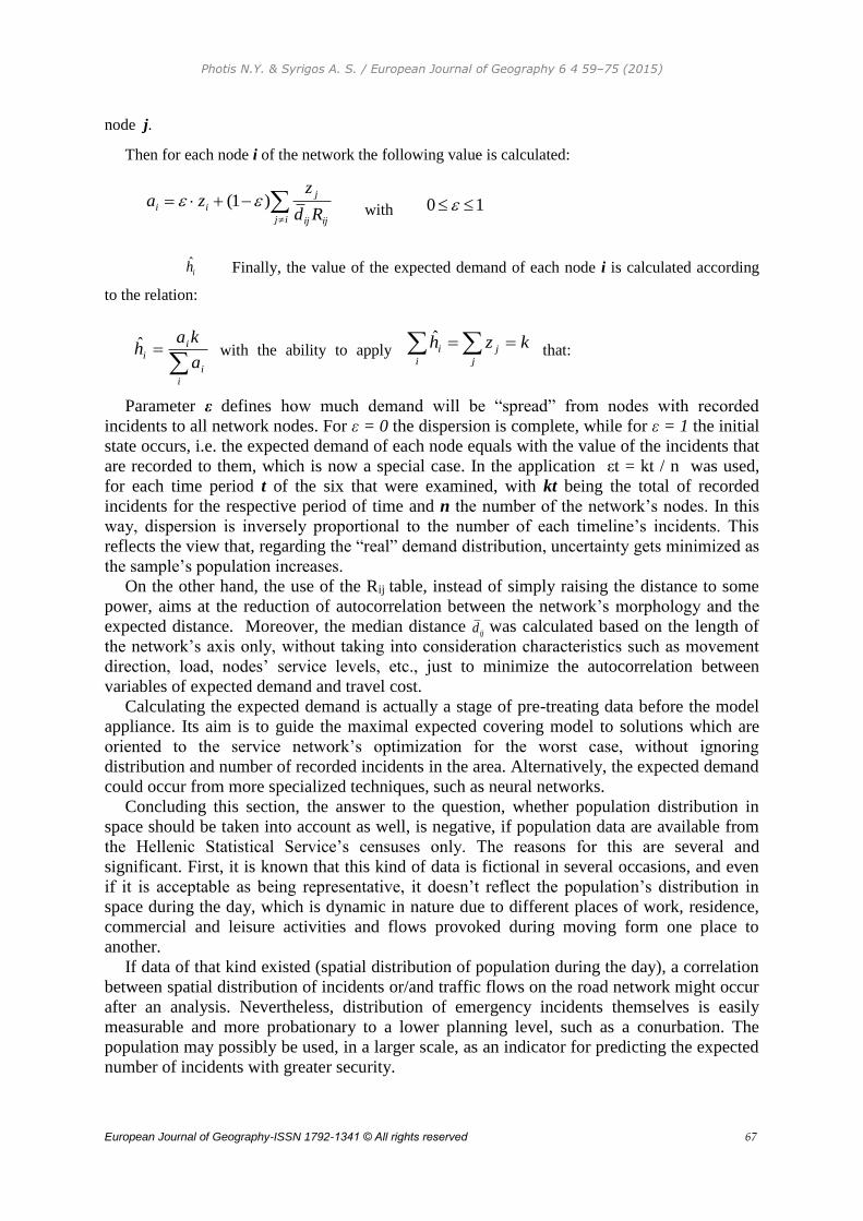
Photis N.Y. & Syrigos A. S. / European Journal of Geography 6 4 59–75 (2015)
European Journal of Geography-ISSN 1792-1341 © All rights reserved 67
node j.
Then for each node i of the network the following value is calculated:
with
Finally, the value of the expected demand of each node i is calculated according
to the relation:
with the ability to apply that:
Parameter ε defines how much demand will be “spread” from nodes with recorded
incidents to all network nodes. For ε = 0 the dispersion is complete, while for ε = 1 the initial
state occurs, i.e. the expected demand of each node equals with the value of the incidents that
are recorded to them, which is now a special case. In the application εt = kt / n was used,
for each time period t of the six that were examined, with kt being the total of recorded
incidents for the respective period of time and n the number of the network’s nodes. In this
way, dispersion is inversely proportional to the number of each timeline’s incidents. This
reflects the view that, regarding the “real” demand distribution, uncertainty gets minimized as
the sample’s population increases.
On the other hand, the use of the Rij table, instead of simply raising the distance to some
power, aims at the reduction of autocorrelation between the network’s morphology and the
expected distance. Moreover, the median distance was calculated based on the length of
the network’s axis only, without taking into consideration characteristics such as movement
direction, load, nodes’ service levels, etc., just to minimize the autocorrelation between
variables of expected demand and travel cost.
Calculating the expected demand is actually a stage of pre-treating data before the model
appliance. Its aim is to guide the maximal expected covering model to solutions which are
oriented to the service network’s optimization for the worst case, without ignoring
distribution and number of recorded incidents in the area. Alternatively, the expected demand
could occur from more specialized techniques, such as neural networks.
Concluding this section, the answer to the question, whether population distribution in
space should be taken into account as well, is negative, if population data are available from
the Hellenic Statistical Service’s censuses only. The reasons for this are several and
significant. First, it is known that this kind of data is fictional in several occasions, and even
if it is acceptable as being representative, it doesn’t reflect the population’s distribution in
space during the day, which is dynamic in nature due to different places of work, residence,
commercial and leisure activities and flows provoked during moving form one place to
another.
If data of that kind existed (spatial distribution of population during the day), a correlation
between spatial distribution of incidents or/and traffic flows on the road network might occur
after an analysis. Nevertheless, distribution of emergency incidents themselves is easily
measurable and more probationary to a lower planning level, such as a conurbation. The
population may possibly be used, in a larger scale, as an indicator for predicting the expected
number of incidents with greater security.
kzhj
j
i
i ˆ
i
i
i
ia
kah
ijd
ih
10
ij ijij
j
iiRd
zza )1(
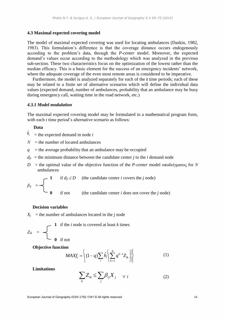
Photis N.Y. & Syrigos A. S. / European Journal of Geography 6 4 59–75 (2015)
European Journal of Geography-ISSN 1792-1341 © All rights reserved 68
4.3 Maximal expected covering model
The model of maximal expected covering was used for locating ambulances (Daskin, 1982,
1983). This formulation’s difference is that the coverage distance occurs endogenously
according to the problem’s data, through the P-center model. Moreover, the expected
demand’s values occur according to the methodology which was analyzed in the previous
sub-section. These two characteristics focus on the optimization of the lowest rather than the
median efficacy. This is a basic element for the success of an emergency incidents’ network,
where the adequate coverage of the even most remote areas is considered to be imperative.
Furthermore, the model is analyzed separately for each of the t time periods; each of these
may be related to a finite set of alternative scenarios which will define the individual data
values (expected demand, number of ambulances, probability that an ambulance may be busy
during emergency call, waiting time in the road network, etc.)
4.3.1 Model modulation
The maximal expected covering model may be formulated in a mathematical program form,
with each t time period’s alternative scenario as follows:
Data
= the expected demand in node i
Ν = the number of located ambulances
q = the average probability that an ambulance may be occupied
dji = the minimum distance between the candidate center j to the i demand node
D = the optimal value of the objective function of the P-center model υποδείγματος for Ν
ambulances
1 if dji D (the candidate center i covers the j node)
βij =
0 if not (the candidate center i does not cover the j node)
Decision variables
Xj = the number of ambulances located in the j node
1 if the i node is covered at least k times
Ζik =
0 if not
Objective function
(1)
Limitations
i (2)
ih
i
ik
N
k
k
it ZqhqMAXf1
1ˆ)1(
j
j
ij
k
ik XZ
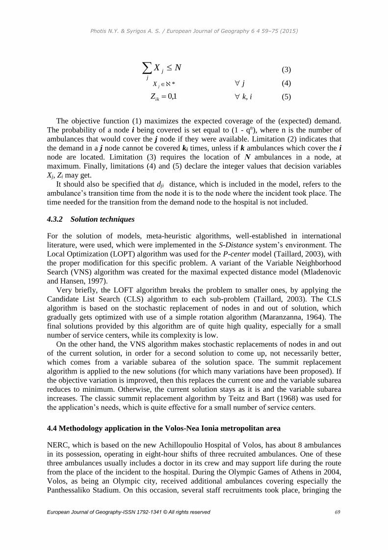
Photis N.Y. & Syrigos A. S. / European Journal of Geography 6 4 59–75 (2015)
European Journal of Geography-ISSN 1792-1341 © All rights reserved 69
(3)
j (4)
k, i (5)
The objective function (1) maximizes the expected coverage of the (expected) demand.
The probability of a node i being covered is set equal to (1 - qn), where n is the number of
ambulances that would cover the j node if they were available. Limitation (2) indicates that
the demand in a j node cannot be covered ki times, unless if k ambulances which cover the i
node are located. Limitation (3) requires the location of Ν ambulances in a node, at
maximum. Finally, limitations (4) and (5) declare the integer values that decision variables
Xj, Zi may get.
It should also be specified that dji distance, which is included in the model, refers to the
ambulance’s transition time from the node it is to the node where the incident took place. The
time needed for the transition from the demand node to the hospital is not included.
4.3.2 Solution techniques
For the solution of models, meta-heuristic algorithms, well-established in international
literature, were used, which were implemented in the S-Distance system’s environment. The
Local Optimization (LOPT) algorithm was used for the P-center model (Taillard, 2003), with
the proper modification for this specific problem. A variant of the Variable Neighborhood
Search (VNS) algorithm was created for the maximal expected distance model (Mladenovic
and Hansen, 1997).
Very briefly, the LOFT algorithm breaks the problem to smaller ones, by applying the
Candidate List Search (CLS) algorithm to each sub-problem (Taillard, 2003). The CLS
algorithm is based on the stochastic replacement of nodes in and out of solution, which
gradually gets optimized with use of a simple rotation algorithm (Maranzanna, 1964). The
final solutions provided by this algorithm are of quite high quality, especially for a small
number of service centers, while its complexity is low.
On the other hand, the VNS algorithm makes stochastic replacements of nodes in and out
of the current solution, in order for a second solution to come up, not necessarily better,
which comes from a variable subarea of the solution space. The summit replacement
algorithm is applied to the new solutions (for which many variations have been proposed). If
the objective variation is improved, then this replaces the current one and the variable subarea
reduces to minimum. Otherwise, the current solution stays as it is and the variable subarea
increases. The classic summit replacement algorithm by Teitz and Bart (1968) was used for
the application’s needs, which is quite effective for a small number of service centers.
4.4 Methodology application in the Volos-Nea Ionia metropolitan area
NERC, which is based on the new Achillopoulio Hospital of Volos, has about 8 ambulances
in its possession, operating in eight-hour shifts of three recruited ambulances. One of these
three ambulances usually includes a doctor in its crew and may support life during the route
from the place of the incident to the hospital. During the Olympic Games of Athens in 2004,
Volos, as being an Olympic city, received additional ambulances covering especially the
Panthessaliko Stadium. On this occasion, several staff recruitments took place, bringing the
1,0ikZ
*jX
NXj
j
Photis N.Y. & Syrigos A. S. / European Journal of Geography 6 4 59–75 (2015)
European Journal of Geography-ISSN 1792-1341 © All rights reserved 70
number of recruited ambulances every time to reach four per shift. NERC’s personnel
admitted that three ambulances are not enough for covering the needs in the conurbation of
Volos, Nea Ionia and the surrounding areas.
4.4.1. Data collection
For the application’s purposes, data was collected in raw (analog) form from the Volos
NERC for the February-August 2004 six-month period. For each recorded incident, only use
of place and time that took place was allowed, and not the incident’s nature. Thus, all
incidents were considered to be equal. In general, in the total of recorded incidents, several of
them didn’t require calling for an ambulance, while incidents in the centers of Volos and Nea
Ionia are more important, according to NERC’s personnel.
Incidents are also separated in (a) urgent, which are covered by NERC’s ambulances
whose base is Volos, (b) urgent, which are covered by ambulances of local health centers and
the hospital of Volos is their destination and (c) evacuations, i.e. patients’ transfer from the
hospital to their homes or transfer of specialized equipment, such as coronary units.
Evacuations are predefined and served by special vehicles and personnel. Therefore, these do
not affect the network’s efficiency. On the other hand, ambulances of local health centers are
sometimes occupied, so the incident must be covered by an NERC’s ambulance, thus
affecting the service network’s efficiency.
Given the fact that this specific application focuses on the urban area of Volos and Nea
Ionia only, the incidents taken into consideration are only those recorded in that area.
Nevertheless, any incidents that take place out of the study area are covered by NERC’s
ambulances, are considered to contribute to the probability of an ambulance being occupied.
For the road network that was used in the application, there was a distinction between 5
categories of roads and bidirectional and one-way movement direction were also taken into
account, service levels of accessible nodes and load, depending on the time period. The final
value introduced to the model is the transfer cost (travel time) in seconds per direction for
each network link. In general, this approach was based on the General Transport and Traffic
Study for the City of Volos (Ministry of Environment, 2008) and on traffic measurements for
the period 2001-2003 as well, which were conducted by students of the Planning and
Regional Development Department, University of Thessaly.
4.4.2 Modulation of alternative scenarios
The analysis that was conducted after the digitization/geocoding of incidents and the
calculation of the expected demand, indicated three important time periods during the day.
The incidents were further separated in two time periods and specifically in weekdays and
holidays/weekends (see Table 1).
One feature that constitutes the different between weekdays and holidays/weekends is the
important increase of incidents that occur outside the study area and are covered by NERC’s
ambulances based in Volos. This is probably due to the exit of a population’s proportion for
leisure purposes.
Besides, the time of the call’s transition to the ambulance and the evaluation of the
traffic’s characteristics in the road network, were considered to be the criteria for the
separation. Especially for the road network, three situations were defined, which represent
two relatively extreme (but not atypical) traffic conditions and an intermediate one.
Then, the maximal expected covering model was solved for each one of the six studied
timer periods for number of ambulances Ν = 3, 4 and 5, while in each one of the eighteen
sub-cases the P-center model was initially solved for the definition of the coverage distance
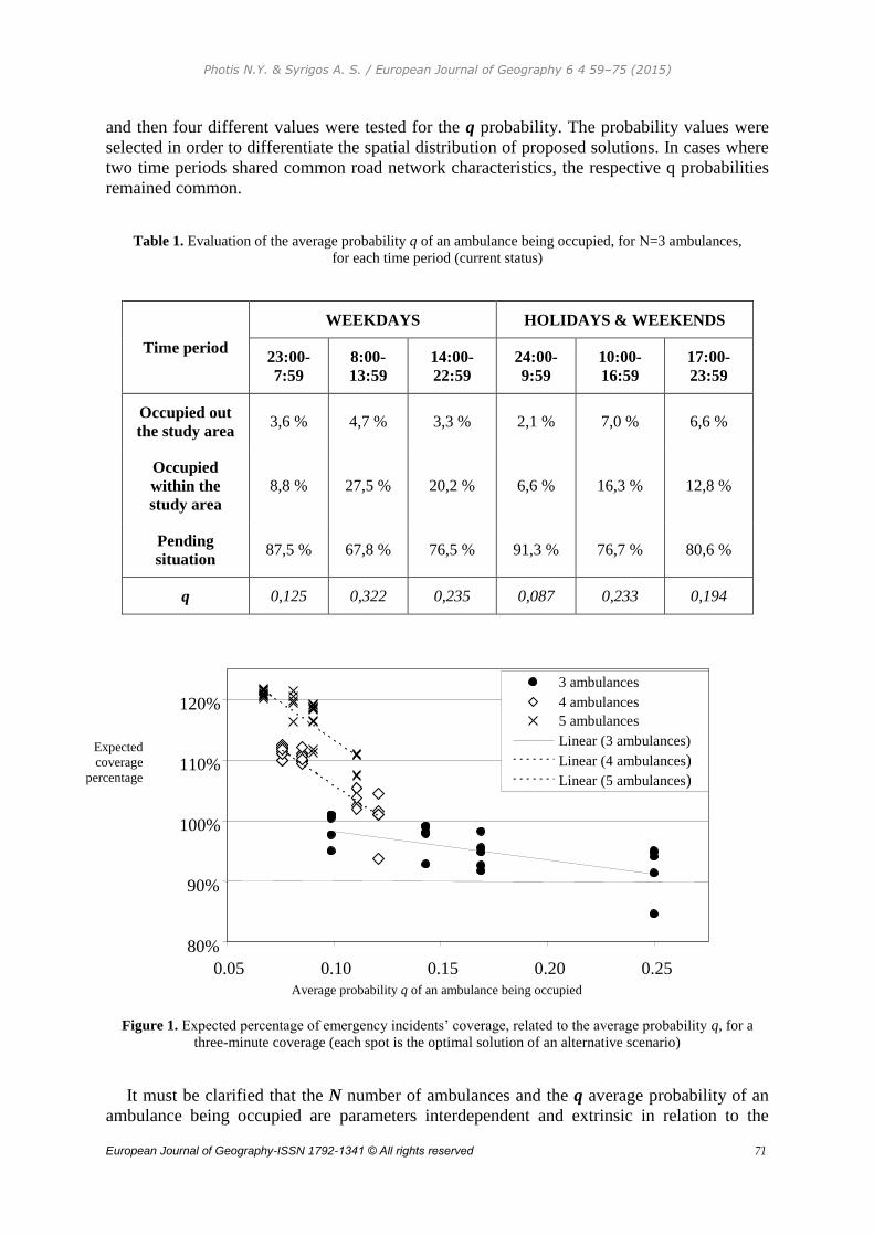
Photis N.Y. & Syrigos A. S. / European Journal of Geography 6 4 59–75 (2015)
European Journal of Geography-ISSN 1792-1341 © All rights reserved 71
and then four different values were tested for the q probability. The probability values were
selected in order to differentiate the spatial distribution of proposed solutions. In cases where
two time periods shared common road network characteristics, the respective q probabilities
remained common.
Table 1. Evaluation of the average probability q of an ambulance being occupied, for Ν=3 ambulances,
for each time period (current status)
Time period
WEEKDAYS HOLIDAYS & WEEKENDS
23:00-
7:59
8:00-
13:59
14:00-
22:59
24:00-
9:59
10:00-
16:59
17:00-
23:59
Occupied out
the study area 3,6 % 4,7 % 3,3 % 2,1 % 7,0 % 6,6 %
Occupied
within the
study area
8,8 % 27,5 % 20,2 % 6,6 % 16,3 % 12,8 %
Pending
situation 87,5 % 67,8 % 76,5 % 91,3 % 76,7 % 80,6 %
q 0,125 0,322 0,235 0,087 0,233 0,194
Figure 1. Expected percentage of emergency incidents’ coverage, related to the average probability q, for a
three-minute coverage (each spot is the optimal solution of an alternative scenario)
It must be clarified that the N number of ambulances and the q average probability of an
ambulance being occupied are parameters interdependent and extrinsic in relation to the
80%
90%
100%
110%
120%
0.05 0.10 0.15 0.20 0.25
Average probability q of an ambulance being occupied
3 ambulances
4 ambulances
5 ambulances
Linear (3 ambulances)
Linear (4 ambulances)
Linear (5 ambulances)
Expected
coverage
percentage

Photis N.Y. & Syrigos A. S. / European Journal of Geography 6 4 59–75 (2015)
European Journal of Geography-ISSN 1792-1341 © All rights reserved 72
model, while in the present application the coverage distance (in seconds) arose
endogenously through the P-center auxiliary model. Altogether, seventy-two alternative
scenarios occurred (ninety with P-center solutions).
One of the main goals was, after the optimal solution of the scenarios above, to find
intermediary solutions through a third model of minimum regret. Regret which is related to a
scenario is calculated by comparing the effectiveness of the optimal location model for the
scenario examined with the effectiveness of the location models resulting from the rest of the
scenarios, if they were applied to the scenario examined (Owen και Daskin, 1998, Snyder,
2005). Therefore, the use of an objective function for minimizing regret may evaluate a
number of robust alternative solutions, based on the optimal values of each initial solution.
5. CONCLUSIONS AND DISCUSSION
The strategic nature of facility location requires methodologies that incorporate, at least up to
a certain point, the uncertainties inherent in real world location problems. For example, many
real world problems exhibit demand-specific uncertainties and uncertainties linked with
transportation costs.
This paper, covered theoretical aspects of static, dynamic and stochastic location-
allocation models whilst focused on the case of the location of ambulances in the
metropolitan area of Volos – Nea Ionia, in Thessaly, Greece. Alternative scenarios were
formulated, which were based on the spatial and temporal distribution of emergency calls, the
spatial and temporal differentiation of network characteristics, the quantity of ambulances
being located and the probability that these ambulances may be busy during an emergency
call arrival.
Furthermore, we introduced S-Distance, a Locational Analysis and Planning Support
System. S-Distance is mainly focused on location-allocation analysis and capable of solving
quite large classical discrete and network locational planning problems based on alternative
scenarios, taking into consideration a variety of social, economic and geospatial variables and
data. Moreover, is a non-commercial Spatial Decision Support System, which incorporates an
interactive solution process within a simplified GIS framework. In this paper, is utilized for
the location of ambulances in the metropolitan area of Volos and Nea Ionia in Greece; the
location-allocation model that was developed, optimizes response for the worst case scenario,
taking into account the stochastic nature as well as the hierarchical structure of the problem,
when considered at the regional or country level. Alternative scenarios are generated based
on the expected geographical and temporal distribution of the emergency incidents (demand),
the traffic flow variability, the number of available ambulances (supply) as well as the
probability an ambulance being occupied on the time of call.
An important finding of our study is that the role of the expected demand was catalytic for
most scenarios. This is apparent particularly where the road network, the coverage distance
and (in most cases) the q probability are common parameters, with the only difference being
the distribution of the expected demand. As shown in Figure 1, for indicative coverage
distance of three minutes, the three ambulances are incapable of serving adequately the
expected demand.
On the other hand, for the same coverage distance, five ambulances cover the expected
demand more than it is needed, regardless of the individual parameters of the alternative
scenarios (the same applies, albeit to a lesser extent, for four ambulances, too). Besides, as q
probability gradually increased, location models tended to be clustered in nodes which
covered the greater demand. This phenomenon is typical of the maximal expected covering
model (Daskin, 1983).

Photis N.Y. & Syrigos A. S. / European Journal of Geography 6 4 59–75 (2015)
European Journal of Geography-ISSN 1792-1341 © All rights reserved 73
The scenarios which theoretically represent more the actual conditions are those where the
q probability is close to the estimated one. Moreover, the quality of scenarios whose
individual variables received the worst values (adverse traffic conditions, increased
probability of occupied ambulances, expected demand in remote nodes), tended to be higher
than the rest of the scenarios. This may apparently be due to the initial selection of optimizing
the service network for the worst case.
Nevertheless, the study’s results are in contradiction with the existing situation. The
location model adopted practically in the study area refers more to the target of optimizing
the average performance of the service network, paying close attention to areas where
incidents took place more often. A possible cause for this is the greater severity of the
incidents recorded in the main part of the conurbation. Another possible case is the available
free space that exists in Volos beach for ambulances parking, which applies to a lesser extent
in areas identified by the model (example, see Map 1).
Furthermore, factors which were not included in the model, such as roadside parking
conditions, could have differentiated the location models which were identified. Finally, the
study area is a subset of the broader region covered by the NERC’s (National Emergency
Response Centre) ambulances, so the two approaches may not be directly comparable.
Nevertheless, the methodology proposed, allows its application to a broader study level (e.g.
regional).
Map 1. Typical existing situation and indicative optimal location for Ν=3 ambulances
Within an integrated emergency incidents’ management approach, of course, apart from
efficient location choices, there is need to balance load of various vehicles, meaning that
continuous indulgence and personnel training, proper function and consultation between
center and vehicles, proper separation of calls to urgent and incidents that may be dealt
locally should be ensured. At the same time, a multi-level service network is required, where

Photis N.Y. & Syrigos A. S. / European Journal of Geography 6 4 59–75 (2015)
European Journal of Geography-ISSN 1792-1341 © All rights reserved 74
personnel of various training levels and capacities will be available, with vehicles of different
equipment and capabilities.
REFERENCES
Averbakh I., (2003). Complexity of robust single facility location problems on networks with
uncertain edge lengths, Discrete Applied Mathematics, 127, pp 505-22.
Batta R., Dolan J.M. and Krishnamurthy N.N., (1989). The maximal expected covering
location problem: Revisited, Transportation Science, 23, pp 277–87.
Church R.L. and ReVelle C.S., (1974). The Maximal Covering Location Model, Papers of
the Regional Science Association, 32, pp 101-18.
Daskin M.S., (1982). Application of an expected covering model to emergency medical
service system design, Decision Sciences, 13, pp 416–39.
Daskin M.S., (1983). A maximum expected covering location model: Formulation properties
and heuristic solution, Transportation Science, 17, pp 48–70.
Daskin M.S., (1995). Network and Discrete Location – Models, Algorithms and Applications,
Wiley Interscience Series, New York.
Daskin, M. S. (2000). A New Approach to Solving the Vertex P-Center Problem to
Optimality: Algorithm and Computational Results. Communications of the Operations
Research Society of Japan, 45(9), 428-436. [1]
Dimopoulou, D., Aggelidou, M., Photis, Y.N., (2015). Up to where a city ends. A
spatiotemporal imprint of commuting patterns for the ten largest Greek cities,
Proceedings of SSS 2015 - 10th International Space Syntax Symposium, pp. 68:1-68:20.
Greek Ministry of Environment, (2006). Transportation analysis for the city of Volos, Athens.
Grekousis, G., Photis, Y.N., (2014). Analyzing High-Risk Emergency Areas with GIS and
Neural Networks: The Case of Athens, Greece, Professional Geographer, 66 (1), pp.
124-137.
Hadjichristodoulou, C., Pournaras, S., Mavrouli, M., Marka, A., Tserkezou, P., Baka, A.,
Billinis, C., Katsioulis, A., Psaroulaki, A., Papa, A., Papadopoulos, N., Mamuris, Z.,
Tsakris, A., Kremastinou, J., Vakalis, N., Koliopoulos, G., Vontas, J., Dovas, C.I.,
Tontis, D., Tselentis, I., Tsiodras, S., Photis, Y.N., Papadopoulou, E., (2015). West nile
virus seroprevalence in the Greek population in 2013: A nationwide cross-sectional
survey, PLoS ONE, 10 (11), pp
Maranzanna F.E., (1964). On the Location of Supply Points to Minimize Transport Costs,
Operations Research Quarterly, 15, pp 261-70.
Mladenović N. and Hansen P., (1997). Variable Neighborhood Search, a Chapter of
Handbook of Metaheuristics, Technical Report: Mathematical Institute, Serbian
Academy of Science, Belgrade. GERAD and Ecole des Hautes Etudes Commerciales,
Montreál.
Mladenović, N., Labbé, M. and Hansen, P. (2003). Solving the p-Center Problem with Tabu
Search and Variable Neighborhood Search. Networks 42(1), 48-64. [2]
Mougiakou, E., Photis, Y.N., (2014). Urban green space network evaluation and planning:
Optimizing accessibility based on connectivity and raster GIS analysis, European
Journal of Geography, 5 (4), pp. 19-46.
Nurković, R., (2015). Contemporary aspects of spatial and urban planning in the Canton of
Sarajevo, European Journal of Geography, 6 (1), pp. 23-36.
Photis N.Y. & Syrigos A. S. / European Journal of Geography 6 4 59–75 (2015)
European Journal of Geography-ISSN 1792-1341 © All rights reserved 75
Owen S.H. and Daskin M.S., (1998). Strategic facility location: A review, European Journal
of Operational Research, 111, pp 423–47.
Papafragkaki, A., Photis, Y.N., (2014). GIS-based location analysis of administrative regions:
Applying the median and covering formulations in a comparative evaluation framework,
European Journal of Geography, 5 (3), pp. 37-59.
Photis Y.N., (2004). Quantitative methods and techniques in facility location, University of
Thessaly Press, Volos (in Greek).
Photis Y.N., (2014). Quantitative Spatial Analysis, Govostis Publishers, Athens.
Photis, Y.N., Grekousis, G., (2012). Locational planning for emergency management and
response: An artificial intelligence approach, International Journal of Sustainable
Development and Planning, 7 (3), pp. 372-384.
Resende, M. G., & Werneck, R. F. (2007). A fast swap-based local search procedure for
location problems. Annals of Operations Research, 150(1), 205-230. [3]
ReVelle C.S. and Eiselt H.A., (2005). Location analysis: A synthesis and survey, European
Journal of Operational Research, 165, pp 1-19.
Roşu, L., Corodescu, E., Blăgeanu, A., (2015). Does geographical location matter? Assessing
spatial patterns in perceived quality of life in European cities, European Journal of
Geography, 6 (2), pp. 15-34.
Sirigos S., (2003). S-Distance: A prototype locational planning decision support system:
Models, algorithms and application, Undergraduate Thesis, University of Thessaly,
Volos (in Greek).
Sirigos S., (2004). Location of facilities and services under uncertainty: Definition of
alternative supply and demand scenarios, Postgraduate Thesis, University of Thessaly,
Volos (in Greek).
Snyder L.V., (2006). Facility location under uncertainty: A review, IIE Transactions, 38(7),
537-554.
Taillard E.D., (2003). Heuristic Methods for Large Centroid Clustering Problems, Journal of
Heuristics, 9, pp 51-74
Teitz M.B. and Bart P., (1968). Heuristic Methods for Estimating Generalized Vertex Median
of a Weighted Graph, Operations Research, 16, pp 955-61.
Weber A., (1909). On the Location of Industries, University of Chicago Press, Chicago.
European Journal of Geography Volume 6, Number 4: 76 – 87, December 2015
©Association of European Geographers
European Journal of Geography-ISSN 1792-1341 © All rights reserved 76
FALLING DOMINOS OR THE ROLE OF GEOGRAPHIC MENTAL MAPS IN
FOREIGN POLICY.
Luis M. DA VINHA Valley City State University, Social Science Department, Valley City, ND USA
http://community.vcsu.edu/facultypages/luis.davinha/My_Webpage/
Abstract
Geographic mental maps are commonly used to explain foreign policy behaviour of political
decision-makers. However, despite the proliferation of their usage, a theoretical account of
how mental maps influence foreign policy is still lacking. The current paper seeks to
contribute to the development of a theoretical framework which can support the use of mental
maps as an analytical concept for foreign policy analysis. Moreover, the paper uses the
domino theory as an example to illustrate how geographic cognition and reasoning effectively
influence foreign policy.
Keywords: beliefs, decision-making, domino theory, foreign policy, geographic mental maps
1. INTRODUCTION
The recent proliferation of studies focusing on political decision-maker’s mental maps testify
to the fundamental role of these geographic constructs in influencing foreign policy-making
(Casey and Wright, 2008; 2011; 2015; Thomas, 2011a; 2011b). Despite their obvious
distortions, few authors would contest that “the decisions that lead to political action,
however, are taken in the more amorphous, nuanced world of the mental map” (Henrikson,
1980: 497). Political decision-makers have to make decisions based on information and
events that are generally outside their national or even regional contexts. Therefore, mental
maps are “systems of orientation” which are used for guidance in foreign policy-making
(Henrikson, 2002).
To make sense of the diversity and complexity of the political world, decision-makers rely
on simplified representations or mental models (Barr et al., 1992; George, 1969; Golledge
and Stimson, 1997; Holsti, 1976; Sapienza, 1987). No one individual can encompass the
complexity of the world in its entirety (Lowenthal, 1961). Scientific studies have established
that individuals and groups have cognitive spatial constructs which they use to simplify
reality and aid political decision-making (Golledge, 2002; Henrikson, 1980; Mark et al.,
1999). Consequently, “the beliefs that compromise these maps provide the individual with a
more or less coherent way of organizing and making sense out of what would otherwise be a
confusing array of signals picked up from the environment by his senses” (Holsti, 2006: 34).
More precisely, decision-makers act with regard to their perceived geographic context,
meaning “what matters in the explanation of decisions and policies is how the actor imagined
his environment to be, not how it actually was” (Sprout and Sprout, 1960: 147). Accordingly,
different actors can respond differently to the same event in the international environment
(Bilgin, 2004; Gould and White, 1974; Jervis, 1976; Kiesler and Sproull, 1982). As a result,
Da Vinha M.L. / European Journal of Geography 6 4 76–87 (2015)
European Journal of Geography-ISSN 1792-1341 © All rights reserved 77
mental maps are essential to policy-making in the sense that they are a “critical component of
general spatial problem-solving activity” (Golledge and Stimson, 1997: 239). By informing
decision-makers about particular geographic settings, mental maps contribute to the process
of spatial choice inherent in foreign policy decision-making.
However, very little research has been devoted to the relationship between geographic
mental maps and political decision-making. The current paper provides an analytical
framework to try to explain the relationship between mental maps and foreign policy. It
begins by employing theoretical assumptions from cognitive and social psychology to
provide some insight on how mental maps influence decision-makers. It subsequently
examines how geographic mental maps guided US foreign policy during the Cold War. More
precisely, the second section demonstrates how particular geographic concepts and reasoning
influenced US policy in Asia, by creating an image of a potential domino effect of communist
expansion in the region.
2. HOW GEOGRAPHIC MENTAL MAPS INFLUENCE FOREIGN POLICY
DECISION-MAKERS
We may define a geographic mental map as a “cognitive representation which encloses an
individual or group’s beliefs about the geographic character of a particular place or places
and their relationship to other places or spatial phenomena” (da Vinha, 2011: 137). The use
of mental maps as an analytical concept has become a commonplace. However, there has
been very little theorizing on how geographic mental maps influence foreign policy decision-
making. Though it is widely accepted that “individuals have cognitive images of places
which they use to simplify reality” and that these “perceptions [are] important in foreign
policy decisionmaking” (O’Loughlin and Grant, 1990: 506), the causal relationship has not
been compellingly demonstrated. In order to understand the role of mental maps on foreign
policy decision-making we will borrow from the theoretical literature on cognitive and social
psychology, particularly regarding beliefs.
The cognitive research agenda has claimed that beliefs, while “subjective representations
of reality”, are important in explaining world politics (Walker and Schafer, 2006). Therefore,
by conceptualizing mental maps as beliefs about geographic phenomena, it seems entirely
logical to assume they affect decision-making in the same manner as belief systems. Beliefs
can be defined as propositions which we assume to be true about causal relationships or
elementary assumptions regarding the way the world functions (Renshon, 2008; Rosati, 1991;
Vertzberger, 2002). The sum of an individual’s beliefs makes up his belief system. In
essence, belief systems comprise all the accumulated and organized knowledge that an
individual possesses about himself and the world (Holsti, 2006; c.f., Rosati, 1991). This
presumes that they are internally consistent, they fluctuate along a central-peripheral
dimension, and they are hierarchically arranged – i.e., the most central beliefs inform the less
central ones (Rosenberg, 1986). However, they surpass mere scientific or social-scientific
knowledge (Jervis, 2006). Emotion is a central factor in understanding beliefs. Therefore,
beliefs can represent inner states as well as outer realities. Also, they can be exhortative,
inciting and encouraging human behaviour. Ultimately, they can acquire a high level of
commitment and faith. As Jervis has exemplified:
When people talk about “beliefs to live by”, moral and empirical considerations are fused.
When people say that they believe that democracy can be brought to the Middle East and that
doing so will make this a better world, they are combining how they see the evidence and
what their values and desires lead them to think should and must be true. (Jervis, 2006: 642)

Da Vinha M.L. / European Journal of Geography 6 4 76–87 (2015)
European Journal of Geography-ISSN 1792-1341 © All rights reserved 78
While a wide range of different types of beliefs have been identified (c.f., Goldstein and
Keohane, 1993), it suffices to know that beliefs contribute to an individual’s understating of
the world. Beliefs help individuals simplify and deal with the complexity of the real world
(however defined and determined) (Holsti, 1976; George, 1969; Jervis, 2006; Renshon,
2008). No one individual can encompass the complexity of the political world in its entirety.
Even large bureaucratic institutions cannot process all the available information and produce
an infallible portrait of the world (Allison and Zelikow, 1999; George, 1969; Henrikson,
1980; Kiesler and Sproull, 1982). To make sense of the diversity and complexities of the
political world, decision-makers rely on simplified representations which help organize all
the intricate variables and give them meaning (Axelrod, 1976; Barr et al., 1992; Golledge and
Stimson, 1997; Holsti, 1976; 2006; Renshon, 2006; 2008; Sapienza, 1987). Accordingly,
beliefs “provide the individual with a more or less coherent way of organizing and making
sense out of what would otherwise be a confusing array of signals picked up from the
environment by his senses” (Holsti, 2006: 34).
As a result, beliefs acquire an important function in foreign policy decision-making. They
simultaneously serve both a descriptive and prescriptive purpose. At the most basic level,
beliefs act as filters through which we manage and interpret incoming information about the
political world (Brodin, 1972; Deutsch and Merritt, 1965; Eidelson and Eidelson, 2003;
Renshon, 2008). Due to their position between the environment and behaviour, beliefs serve
as relatively stable templates which help individuals select, organize, process, and understand
the plethora of signals they receive (George, 1980; Rosati, 1991; 2005).
Beliefs comprise assimilation and appraisal mechanisms that aid individuals in
assimilating new information within existing knowledge and representing it in ways which
reduce conflict with expectations – i.e., beliefs help individuals maintain their quality of
“consistency seekers” (George, 1980; Holsti, 2006; Jervis, 2006). First of all, expectations
play an important role in interpreting information; people tend to perceive events in
accordance with their existing beliefs. Thus, beliefs help individuals maintain a high degree
of cognitive consistency (Jervis, 1976). Furthermore, incoming information is also more
easily integrated when it is considered plausible and resonates with existing beliefs. As
Vertzberger has (2002: 117) has indicated “when the core beliefs of another person or actor
are in line with one´s own, one tends to see them as even closer than they actually are”. In
contrast, when beliefs are divergent, they tend to be discounted and perceived as “much more
dissimilar and incongruent than they actually are (Vertzberger, 2002: 117). Equally
important, ambiguous information is generally considered consistent with existing beliefs
and, in the majority of the cases, reinforces individual’s prior convictions.
In their prescriptive role, beliefs provide orientation guides for behaviour. By providing
norms and standards for action, beliefs stipulate what George (1940) has termed “choice
propensities” which bound the policy choices available to decision-makers. While not
completely determining behaviour, beliefs do serve as “road maps” (Goldstein and Keohane,
1993) which lay down the moral and ethical boundaries for political action. Therefore, they
can they can determine “what is right and wrong, provide new social visions, or merely
suggest what economic policy will steer a nation towards increased wealth” (Goldstein and
Keohane, 1993: 16). Equally, beliefs can provide key “focal points” that allow various
individuals to rally around and act upon. Beliefs can also be embedded in institutional
frameworks, generalizing rules and actions and associating diverse issues. Once beliefs are
institutionalized they tend to constrain policy in the absence of innovation. In other words,
once beliefs are entrenched in organizational and normative structures “that policy idea can
affect the incentives of political entrepreneurs long after the interests of its initial proponents
have changed” (Goldstein and Keohane, 1993: 13).
Da Vinha M.L. / European Journal of Geography 6 4 76–87 (2015)
European Journal of Geography-ISSN 1792-1341 © All rights reserved 79
By providing a number of different cognitive cues these various features facilitate the
decision-making process by abridging the complexity involved in foreign policy decision-
making (Rosati, 2000). Accordingly, beliefs can act upon individual´s behaviour through a
wide gamut of formulas, but this does not imply that they mechanically affect foreign policy
decision-making. The role of beliefs in foreign policy decision-making is not as
straightforward and direct as many assume. Their influence is more subtle and discreet. By
affecting the way individuals define the situation they indirectly condition the options for
action.
Rather than acting as direct guides to action, they form one of a several clusters of intervening
variables that may shape and constrain decision-making behaviour. They may serve the policy
makers as a means of orienting him to the environment; as a lens or prism through which
information is processes and given meaning; as a diagnostic scheme; as one means of coping
with the cognitive constraints on rationality; as a source of guidelines that may guide or
bound – but not necessarily determine – policy prescriptions and choices. Thus, attention
should be directed to the linkages between beliefs and certain decision-making tasks that
precede a decision – definition of the situation, analysis, prescription, and the like. (Holsti,
1976: 34-35)
In effect, it is precisely in the definition of the situation (i.e., the problem representation)
that geographic mental maps contribute to foreign policy decision-making, for it has been
accepted that “the initial problem representation strongly constrains subsequent behavior”
(Taber, 1998: 26; c.f., Sylvan, 1998; Vertzberger, 2002; Voss, 1998). More precisely, when a
problematic state of affairs arises in international politics, decision-makers develop a problem
representation in congruence with their knowledge and beliefs (Beasley, 1998; Voss, 1998).
This representation is an essential part of the information processing stage of foreign policy
decision-making. Its significance derives from the fact that it helps recognize and concentrate
on incoming information, evaluate its relevance to the problem under consideration, and
integrate it into the existing knowledge structure (Vertzberger, 2002).
Accordingly, when an individual has to make a spatial decision, his mental map is
“triggered”, allowing him to make sense of the diversity and complexities of his environment
by cognitively categorizing, associating, and ordering disparate geographic information
(Golledge, 2002; Henrikson, 1980; Mark et al., 1999). In other words, the complexity
resulting from the various geographic factors present in a specific place is abridged in order
to be manageable and intelligible to individual decision-makers. In this sense they help
mediate our geographic beliefs about the world.
This capacity to simplify geographic complexities is accomplished through what Golledge
and Stimson (1997: 32) have designated as the “first motivated response” which is
responsible for activating the decision-making process. Accordingly, a particular event in the
international environment can provide a stimulus for decision-makers to act – i.e., the first
motivated response. This naturally implies a search for information. Seeking out relevant
information is not a straight-forward, rationally inspired process. On the contrary, the search
for information is regularly guided by personal or organizational objectives and expectations
and, as mentioned above, suffers from many cognitive constraints that lead to selectivity of
the information. The ill-defined nature of problems, characteristic of international politics,
makes selecting relevant information even more complicated. As a result:
When ill-defined problems compete for attention with well-defined and structured problems,
the later often distract attention from the former. Decisionmakers prefer to deal with what
seems manageable rather than with what is ambiguous even if it is possibly more important
and potentially dangerous. Yet decisionmakers are not always aware of the differences
Da Vinha M.L. / European Journal of Geography 6 4 76–87 (2015)
European Journal of Geography-ISSN 1792-1341 © All rights reserved 80
between well-defined and ill-structured problems. In fact they unconsciously transform ill-
structured problems into well defined ones by ignoring their distinct attributes. (Vertzberger,
2002: 54)
An additional procedure of the first motivated response is the development of an
individual’s behaviour-space perception (Golledge and Stimson, 1997). This process involves
selecting information, of either spatial or non-spatial quality, from an individual’s existing
mental maps, usually located in his long-term memory. The reason for this process is that, as
stated above, the information received from the environment is normally vague and imprecise
and, consequently, individuals need their pre-existing knowledge and beliefs to make sense of
the incoming inputs (Taber, 1998). Thus, the non-spatial attributes may comprise a wide
array of features relating to a specific place or space of an event such as regime type, military
strength, economic development, institutional association, religion, etc. For their part, the
spatial attributes permit individuals to locate and order the features and initiate spatial
correlations.
Once the assorted information is assembled, the mental map can then be activated for
processing. This implies that components of the stored mental maps are transmitted from the
long-term memory to the working memory in order to be processed in accordance with the
decision-making criteria necessary to solve the particular problem under consideration. The
array of geographic knowledge available in our long-term memory results from the fact that
individuals have countless geographic mental maps. In fact, individuals store multiple
representations of their geographic environments (Battersby and Montello, 2009; Tversky,
2003; Tversky et al, 1994) which has allowed Downs and Meyer (1978: 68) to speak of
mapping rather than maps, for what is at stake is “the capacity to generate a representation of
the spatial environment… representing some part of the world at one instance in time”. The
geographic information evoked at any given moment depends on the nature of the task at
hand. Accordingly, Walker (2000) has identified an assemblage of different mental maps
which policy-makers use to help them come to a decision: security maps; economic maps;
cultural maps; religious maps; geographic maps; and political maps. The entire assortment of
these different mental maps compromise an individual’s world view (Peuquet, 2002).
3. MAPPING FALLING DOMINOS
As noted above, instead of passively reflecting the political environment, geographic mental
maps steer foreign policy decisions by shaping policy-maker’s perceptions, acting as
mechanisms of cognitive and motivated bias that distort, block, and recast incoming
information. An example of how geographic mental maps affect foreign policy is vividly
illustrated by George Ball’s recollection of the US policy towards Southeast Asia:
We can live with the Vietnam war so long as we remember that it is a peripheral contest, but
we do not always act as if we thought so. Sometimes we behave as though Southeast Asia did
lie at the center of power (…) but any shooting war takes a large toll in the emotions of the
public and the attention of the top government leaders who are responsible for navigating the
ship of state in international waters. Moreover, it tends to confuse priorities and leads to
navigation by a distorted chart – like something drawn by a medieval cartographer, in which
Vietnam appears as a major continent lying just off our shores and threatening our national
existence. (Ball, 1968: 351-352)
Ball’s words testify to Cottam and McCoy’s (1998) assertion that the Cold War was a
cognition-dominated conflict. Central to US involvement in Vietnam and Southeast Asia was
Da Vinha M.L. / European Journal of Geography 6 4 76–87 (2015)
European Journal of Geography-ISSN 1792-1341 © All rights reserved 81
a specific geographic cognition that emphasized certain threats and opportunities over others
– i.e., the domino effect. Since the end of the 2nd World War, the domino theory has
underpinned US foreign policy in the Third World (Slater, 1987). But nowhere has it been
more compelling than in the case of the US intervention in Vietnam. While there where
certainly many other rationalizations for US involvement in Vietnam – .e.g., the safeguard of
freedom and democracy, upholding of self-determination, upkeep of US commitments to its
allies (SEATO) – none was more determinant the domino theory (Slater, 1993).The
underlying logic of the domino theory has a long standing tradition in international politics.
Geopolitical reasoning is filled with the principle convictions of the domino effect. Lord
Salisbury reasoned in the mid-nineteenth century “that Russia was in Armenia, that Armenia
is the key to Syria, that Syria is the Key to Egypt, and that anyone advancing into Egypt has
the key to Africa” (cited in Jervis, 1991: 21). No one, however, has had more success
promulgating the theory’s underlying principles than Halford Mackinder (1996). His
heartland theory rested on the basic assumption that he who controlled East Europe would
ultimately dominate global politics. Thus, it is not surprising that the logic of the domino
theory found such receptivity in US decision-makers.
In very broad terms, the domino theory asserts that a defeat or retreat in one area of the
world would produce further demands and aggression by adversaries in other areas. While, as
affirmed above, the logic of the falling dominos has a long tradition in foreign policy
rationalizations, it was the events in Asia that consolidated its validity it in the minds of US
decision-makers (Glad and Taber, 1990; Jervis, 1980). President Eisenhower (1954) set down
the principles in a press conference by insisting that in Indochina “You have a row of
dominoes set up, you knock over the first one, and what will happen to the last one is the
certainty that it will go over very quickly”. Prior to the Korean War, the US had
discriminated between areas of high strategic value and ones of more peripheral interest
(Gaddis, 2005; Jervis, 1980). As instability grew and friendly regimes were challenged
throughout the region, this dichotomy vanished. Every area was now of vital interest for
America and their defence against communist expansion was of strategic significance.
However, the application of the domino theory to Vietnam evoked an inevitable tragic
blow for US interests. Any concession in the region was deemed to be a major forfeiture of
America’s global standing:
The fall of Vietnam would cause the loss of all Indochina and then the rest of Southeast Asia,
with implications extending far beyond. The communists had just taken over in China.
Indochina, Burma and Malaya were swept by revolution, and the newly independent
government of Indonesia seemed vulnerable. Because of its location on China's southern
border and because it appeared in the most imminent danger, Vietnam was considered crucial.
If it fell, all of Southeast Asia might be lost, denying the United States access to important
raw materials and strategic waterways. (Herring, 1991: 107)
While US officials never truly offered a conceptual description of how the theory was
applied in practice, it is possible, however, work out some of the basic assumptions or causal
links that supported its claims (Glad and Taber, 1990; Slater, 1987; 1993). To begin with,
revolutions – specifically communist revolutions – were considered to be externally guided
events, sponsored by the Soviet Union. Secondly, the Soviets challenged the US on
peripheral issues in order to test its determination to resist. In other words, instead of overtly
challenging the US, the Soviets would promote subversive activities in areas of allegedly
marginal interest for the US.
Da Vinha M.L. / European Journal of Geography 6 4 76–87 (2015)
European Journal of Geography-ISSN 1792-1341 © All rights reserved 82
Another fundamental assumption was the direct relationship between revolutions in one
country and revolutions in its adjacent region. The contagion effect was quite straightforward
and it was perceived that “successful revolutions quickly spread, both because of an
emulation effect and because revolutions actively seek to export themselves” (Slater, 1987:
107). Underlying this belief is a basic geographic reasoning based on the primitives of spatial
knowledge, particularly those associated with proximity, connection, and linkage (c.f.,
Golledge, 1995).
From this postulation it followed that the US had to act quickly and decisively in order to
contain the spread of the revolutionary malaise. The common understanding was that
standing up to the aggressor would cause them to yield from their expansionary activities.
Should the US fail to meet the aggressor’s challenge, even in a traditionally insignificant
country, it would lead to the fall of the entire region and put vital US interests and American
national security at stake. While the domino theory never actually established the causality
between the fall of a region and the endangerment to US national security, the basic
assumption was that the failure to respond to the threat would undermine US credibility
worldwide. Above all, it would encourage less powerful states to accommodate to Soviet
expansion as well as embolden the Soviet expansionist fervour:
The integrity of the US commitment is the principal pillar of peace throughout the world. (…)
If that commitment becomes unreliable, the communist world would draw conclusions that
would lead to our ruin and almost certainly to a catastrophic war. (Rusk cited in Gaddis,
2005: 238).
The veracity of these assumptions has been amply debated and it is generally accepted that
they do not resist empirical scrutiny (Glad and Taber, 1990; Slater, 1987; 1993). However,
the validity of the domino theory is of no interest to the present study. Rather, it suffices to
acknowledge that the domino theory offered US foreign policy decision-makers a
geographically-inspired framework which they could use to understand international events
and respond to them. Whereas Slater (1987: 130; 1993) denunciates the domino theory as a
combination of analogy and ideology which was used to “justify a policy of indiscriminate
global anticommunism”, we rather prefer to understand it as a collection of beliefs about the
international environment and politics. As a matter of fact, instead of a theory, Jervis (1991)
identifies “domino beliefs” that ultimately encompassed propositions about the way the
revolutions in foreign countries worked and what the adequate policy responses should be.
According to Glad and Taber (1990: 63), the domino theory, “provided American decision
makers with a map explaining their new world”. This map not only exposed the problem at
hand, but also “suggested simple prescriptions for dealing with the threat” (Glad and Taber,
1990: 63).
In reality, the domino theory incorporated a wide range of geographic mental maps that
comprised a set of geographic beliefs that helped decision-makers define the problem
representation. The most obvious geographic beliefs involved a great deal of spatial
reasoning. More precisely, spatial concepts such as contiguity, sequence, connection and
linkage, boundary, dispersion, and pattern were all involved in the domino theory. The
mental maps of US decision-makers portrayed a centre of hostility – i.e., the Soviet Union –
that was pushing outward, gulping up entire countries until it would circumscribe US vital
interests. A mechanical-like process would propagate communist insurrections from country
to country, crafting a regional arrangement of Soviet dominated regimes. The revolutionary
impulse would be unfettered by natural topographies, national boundaries, or even local
Da Vinha M.L. / European Journal of Geography 6 4 76–87 (2015)
European Journal of Geography-ISSN 1792-1341 © All rights reserved 83
specificities. One by one each country would inevitably fall to the revolutionary impulse.
Only quick and strong intervention from the US could possibly halt the communist tide.
The implications of this rationale are quite revealing from a holistic geographic
perspective. What it reveals is an overarching mental map that distorted and oversimplified
the political environment in order for decision-makers to cope with its complexity. First of
all, the dominant geographic mental maps identified a single, monolithic threat to the US –
i.e., the USSR. The Soviets, according to official accounts, had an imperial agenda which
culminated in the eradication of any alternative models of society. This agenda proposed an
expansionist policy which sought to enlarge Soviet control over other territories, namely
through the subversion of foreign regimes. Since the USSR commanded international
communism, this left no margin for any autonomous action on the part of other national
communist movements. Therefore, the threat to the US became geographically homogenized,
meaning that since the Soviets were behind every revolution it was impossible to distinguish
between places of central and peripheral interest. And since what generally “makes an
interest or a geographical area essential is the fact that it is threatened by an adversary”
(Jervis, 1991: 24) any area facing a communist uprising was deemed of primal significance.
What is even more revealing is how US decision-makers regarded the local political
situation. The people of Southeast Asia were cleansed of any political autonomy. Not only
were the local populations and political officials easy prey for communist machinations, but
they were also powerless to resist such aggression. Without strong and determined US
involvement local resistance would collapse and accommodate to Soviet rule. As pointed out
above, geographic mental maps also serve the purpose of characterizing the people of foreign
lands. Of the most unrelenting ideas is that “some places are inhabited by normal human
beings, much like ourselves, while other places are inhabited by barbarians” (Elliot, 1979:
250; c.f., Latham, 2001). In Southeast Asia and particularly in Vietnam, the geographic
mental maps of US officials depicted a fragile and vulnerable people that required US
protection and involvement in order to repel aggression. From this perspective, geography
can conjure up images of either fear or hope (Sparke, 2007) which consequently condition the
policy options. The geographic mental maps of US decision-makers were certainly maps of
fear, which highlighted endless threats and risks. However, the problem representation
rendered by the geographic mental maps also framed the possible course of actions. The
policy options were conditioned a priori:
If the domino theory explained why it was important to prevent even small forceable changes
in the status quo, the emerging theory of deterrence explained why it was possible to do so.
This theory argues that when war is the worst possible outcome for both sides, a state can
prevail by committing itself to stand firm – by staking its reputation on not giving in. (Jervis,
1980: 582)
Accordingly, the US mental maps revealed as much about the beliefs of the US as it did
about Southeast Asia. Ultimately, “what was at stake in Vietnam was not ʻnational securityʼ
but rather America's image of itself as a global power (Slater, 1993: 215). In this sense, the
US was imperilled by the massive threat of Soviet communism. It was at a disadvantage vis-
à-vis the USSR and was apprehensive of the future. Not only would the US have to step up to
the challenge, but it would have to do it unaided. Consequently, only a determined and fully
committed US could deter the Soviet expansion. Any hesitation would undermine US
security for no other force could prevent the communist onslaught from bordering the
American shores. In fact, the mental maps underlying US foreign policy bare a very isolated
and alarmed superpower.
Da Vinha M.L. / European Journal of Geography 6 4 76–87 (2015)
European Journal of Geography-ISSN 1792-1341 © All rights reserved 84
4. CONCLUSIONS
Mental maps are useful analytical concepts for analysing foreign policy (c.f., da Vinha,
2011). However, much theoretical work is still required to fully exploit their analytical
potential. In particular, the mental map research agenda requires a substantial theorising
enterprise which can help us better understand the dynamics and mechanisms involved in
influencing decision-makers. In addition, the geographic elements underscoring mental maps
have to be clarified. Political science, and International Relations in particular, lack a clear
appreciation of geography. Recent research testifies to the continued primacy of the
determinants of physical geography and spatial reasoning in analysing international politics
(c.f., Kaplan, 2009).
The requirements for such an undertaking should not be underestimated. Current
international politics continue to be influenced by decision-maker’s mental maps. Geographic
considerations such as those inspiring the domino theory continue to exercise their sway over
foreign policy-makers. For example, recent events in the greater Middle East testify to this
rationale. For some, the forced democratization of Iraq or the endogenous democratic
uprisings in a few countries would transform the political landscape of the entire region. For
others, the threat of state-failure and the growth of the non-state terrorist entities would have
devastating consequences for the entire region and its immediate periphery. In each case,
once the first domino falls, the rest would follow. The veracity of such claims are irrelevant.
Policy decisions are made according to the decision-maker’s beliefs regarding the existing
situation and the potential outcomes of their policy options. Understanding how our
geographic mental maps shape our decisions is of greater importance, for it can shine insight
not only on how we view others, but also how we view ourselves.
REFERENCES
Allison, Graham and Zelikow, Philip. 1999. Essence of Decision: Explaining the Cuban
Missile Crisis. New York: Longman.
Axelrod, Robert. 1976. The Cognitive Mapping Approach to Decision Making. In Structure
of Decision: The Cognitive Maps of Political Elites, Axelrod, R. (Ed.), 3-17. Princeton,
NJ: Princeton University Press.
Ball, George. 1968. The Discipline of Power: Essentials of a Modern World Structure.
Boston: Little, Brown and Company.
Barr, Pamela; Stimpert, John and Huff, Anne. 1992. Cognitive Change, Strategic Action, and
Organizational Renewal, Strategic Management Journal. 13 (1): 15-36.
Battersby, Sarah and Montello, Daniel. 2009. Area Estimation of World Regions and the
Projection of the Global-Scale Cognitive Map, Annals of the Association of American
Geographers. 99 (2): 273-291.
Beasley, Ryan. 1998. Collective Interpretations: How Problem Representations Aggregate in
Foreign Policy Groups. In Problem Representation in Foreign Policy Decision Making,
Sylvan, D. and Voss, J. (Eds.), 80-115. Cambridge: Cambridge University Press.
Bilgin, Pinar. 2004. Whose ‘Middle East’? Geopolitical Inventions and Practices of Security,
International Relations. 18 (1): 25-41.
Brodin, Katarina. 1972. Belief Systems, Doctrines, and Foreign Policy: A Presentation of
Two Alternative Models for the Analysis of Foreign Policy Decision-making,
Cooperation and Conflict. 7: 97-112.
Da Vinha M.L. / European Journal of Geography 6 4 76–87 (2015)
European Journal of Geography-ISSN 1792-1341 © All rights reserved 85
Casey, Steven and Wright, Jonathan (Eds.). 2008. Mental Maps in the Era of Two World
Wars. New York: Palgrave-Macmillan.
Casey, Steven and Wright, Jonathan (Eds.). 2011. Mental Maps in the Early Cold War Era,
1945-1968. New York: Palgrave-Macmillan.
Casey, Steven and Wright, Jonathan (Eds.). 2015. Mental Maps in the Era of Détente and the
End of the Cold War 1968-91. New York: Palgrave-Macmillan.
Cottam, Martha and McCoy, Dorcas. 1998. Image Change and Problem Representation after
the Cold War. In Problem Representation in Foreign Policy Decision Making, Sylvan,
D. and Voss, J. (Eds.), 116-144. Cambridge: Cambridge University Press.
da Vinha, Luis. 2011. Assessing the Conceptual ‛Goodness’ of Geographic Mental Maps for
Foreign Policy Analysis, Romanian Review on Political Geography. 13 (2): 133-148.
Deutsch, Karl and Merritt, Richard. 1965. Effects of Events on National and International
Images. In International Behavior: A Social-Psychological Analysis, Kelman, H. (Ed.).
New York: Holt, Rinehart, and Winston.
Downs, Roger and Meyer, James. 1978. Geography and the Mind: An Exploration of
Perceptual Geography, American Behavioral Scientist. 22 (1): 59-77.
Eidelson, Roy and Eidelson, Judy. 2003. Dangerous Ideas: Five Beliefs that Propel Groups
Toward Conflict, American Psychologist. 58 (3): 182-192.
Eisenhower, Dwight. 1954. The President's News Conference. Available at
http://www.presidency.ucsb.edu/ws/index.php?pid=10202&st=&st1=.
Elliot, Harold. 1979. Mental Maps and Ethnocentrism: Geographic Characterizations in the
Past, Journal of Geography. 78 (7): 250-265.
Gaddis, John Lewis. 2005. Strategies of Containment: A Critical Appraisal of American
National Security Policy during the Cold War. New York: Oxford University Press.
George, Alexander. 1969. The ‘Operational Code’: A Neglected Approach to the Study of
Political Leaders and Decision-Making, International Studies Quarterly. 13 (2): 190-
222.
George, Alexander. 1980. Presidential Decisionmaking in Foreign Policy: The Effective Use
of Information and Advice. Boulder, CO: Westview Press.
Glad, Betty and Taber, Charles. 1990. Images, Learning, and the Decision to Use Force: The
Domino Theory of the United States. In Psychological Dimensions of War, Glad, B.
(Ed.), 56-81. Newbury Park, CA: Sage Publications.
Goldstein, Judith and Keohane, Robert. 1993. Ideas and Foreign Policy: An Analytical
Framework. In Ideas and Foreign Policy: Beliefs, Institutions, and Political Change,
Goldstein, J. and Keohane, R. (Eds.), 3-10. New York: Cornell University Press.
Golledge, Reginald and Stimson, Robert. 1997. Spatial Behavior: A Geographic Perspective.
New York: The Guilford Press.
Golledge, Reginald. 1995. Primitives of Spatial Knowledge. In Cognitive Aspects of Human-
Computer Interaction for Geographic Information Systems, Nyerges, T; Mark, D;
Laurini, R; and Egenhofer, M. (Eds.), 29-44. Dordrecht, Netherlands: Kluwer Academic
Publishers.
Golledge, Reginald. 2002. The Nature of Geographic Knowledge, Annals of the Association
of American Geographers. 92 (1): 1-14.
Da Vinha M.L. / European Journal of Geography 6 4 76–87 (2015)
European Journal of Geography-ISSN 1792-1341 © All rights reserved 86
Gould, Peter and White, Rodney. 1974. Mental Maps. Middlesex: Penguin Books.
Henrikson, Alan. 1980. The Geographical ‘Mental Maps’ of American Foreign Policy
Makers, International Political Science Review. 1 (4): 495-530.
Henrikson, Alan. 2002. Distance and Foreign Policy: A Political Geography Approach,
International Political Science Review. 23 (4): 437-466.
Herring, George. 1991. America and Vietnam: The Unending War, Foreign Affairs. 70 (5):
104-119.
Holsti, Ole. 1976. Foreign Policy Formation Viewed Cognitively. In Structure of Decision:
The Cognitive Maps of Political Elites, Axelrod, R. (Ed.), 18-54. Princeton, NJ:
Princeton University Press.
Holsti, Ole. 2006. Making American Foreign Policy. New York: Routledge.
Jervis, Robert. 1976. Perception and Misperception in International Politics. Princeton, NJ:
Princeton University Press.
Jervis, Robert. 1980. The Impact of the Korean War on the Cold War. The Journal of Conflict
Resolution. 24 (4): 563-592.
Jervis, Robert. 1991. Domino Beliefs and Strategic Behavior. In Dominoes and Bandwagons:
Strategic Beliefs and Great Power Competition in the Eurasian Rimland, Jervis, R. and
Snyder, J. (Eds.), 20-50. New York: Oxford University Press.
Jervis, Robert. 2006. Understanding Beliefs, Political Psychology. 27 (5): 641-663.
Kaplan, Robert. 2009. The Revenge of Geography, Foreign Policy. 96-105.
Kiesler, Sara and Sproull, Lee. 1982. Managerial Response to Changing Environments:
Perspectives on Problem Sensing from Social Cognition, Administrative Science
Quarterly. 27 (4): 548-570.
Latham, Andrew. 2001. China in the Contemporary American Geopolitical Imagination,
Asian Affairs: An American Review. 28 (3): 138-145.
Mackinder, Halford. 1996. Democratic Ideals and Reality: A Study in the Politics of
Reconstruction. Washington, DC: National Defense University Press.
Mark, David; Freksa, Christian; Hirtle, Stephen; Lloyd, Robert and Tversky, Barbara. 1999.
Cognitive Models of Geographical Space, International Journal of Geographical
Information Science. 13 (8): 747-774.
O’Loughlin, John and Grant, Richard. 1990. The Political Geography of Presidential
Speeches, 1946-87, Annals of the Association of American Geographers. 80 (4): 504-
530.
Peuquet, Donna. 2002. Representations of Space and Time. New York: The Guildford Press.
Renshon, Jonathan. 2006. Why Leaders Choose War: The Psychology of Prevention.
Westport, CT: Praeger Security International.
Renshon, Jonathan. 2008. Stability and Change in Belief Systems: The Operational Code of
George W. Bush, Journal of Conflict Resolution. 52 (6): 820-894.
Rosati, Jerel. 1991. The Carter Administration’s Quest for Global Community: Beliefs and
their Impact on Behavior. Columbia, SC: University of South Carolina Press.
Da Vinha M.L. / European Journal of Geography 6 4 76–87 (2015)
European Journal of Geography-ISSN 1792-1341 © All rights reserved 87
Rosati, Jerel. 2000. The Power of Human Cognition in the Study of World Politics,
International Studies Review. 2 (3): 45-75.
Rosenberg, J Philipp. 1986. Presidential Beliefs and Foreign Policy Decision-Making
Continuity during the Cold War Era, Political Psychology. 7 (4): 733-751.
Sapienza, Alice. 1987. Imagery and Strategy, Journal of Management. 13 (3): 543-555.
Slater, Jerome. 1987. Dominos in Central America: Will They Fall? Does It Matter?,
International Security. 12 (2): 105-134.
Slater, Jerome. 1993. The Domino Theory and International Politics: The Case of Vietnam,
Security Studies. 3 (2): 186-224.
Sparke, Matthew. 2007. Geopolitical Fears, Geoeconomic Hopes, and the Responsibilities of
Geography, Annals of the Association of American Geographers. 97 (2): 338-349.
Sprout, Harold and Sprout, Margaret. 1960. Geography and International Politics in an Era of
Revolutionary Change, Journal of Conflict Resolution. 4 (1): 145-161.
Sylvan, Donald. 1998. Introduction. In Problem Representation in Foreign Policy Decision
Making, Sylvan, D. and Voss, J. (Eds.), 3-7. Cambridge: Cambridge University Press.
Taber, Charles. 1998. The Interpretation of Foreign Policy Events: A Cognitive Process
Theory. In Problem Representation in Foreign Policy Decision Making, Sylvan, D. and
Voss, J. (Eds.), 29-52. Cambridge: Cambridge University Press.
Thomas, Martin (Ed.). 2011a. The French Colonial Mind, Volume 1: Mental Maps of Empire
and Colonial Encounters. Lincoln, NE: University of Nebraska Press.
Thomas, Martin (Ed.). 2011b. The French Colonial Mind, Volume 1: Mental Maps of Empire
and Colonial Encounters. Lincoln, NE: University of Nebraska Press.
Tversky, Barbara. 2003. Structures of Mental Spaces: How People Think About Space,
Environment and Behavior. 35 (1): 66-80.
Tversky, Barbara; Franklin, Nancy; Taylor, Holly and Bryant, David. 1994. Spatial Mental
Models from Descriptions, Journal of the American Society for Information Science. 45
(9): 656-668.
Vertzberger, Yaacov. 2002. The World in their Minds: Information Processing, Cognition
and Perception in Foreign Policy Decisionmaking. Stanford, CA: Stanford University
Press.
Voss, James. 1998. On the Representation of Problems: An Information-Processing
Approach to Foreign Policy Decision Making. In Problem Representation in Foreign
Policy Decision Making, Sylvan, D. and Voss, J. (Eds.), 8-26. Cambridge: Cambridge
University Press.
Walker, Martin. 2000. Variable Geography: America’s Mental Maps of Greater Europe,
International Affairs. 76 (3): 459-474.
Walker, Stephen and Schafer, Mark. 2006. Belief Systems as Causal Mechanisms in World
Politics: An Overview of Operational Code Analysis. In Beliefs and Leadership in World
Politics: Methods and Applications of Operational Code Analysis, Schafer; M. and
Walker, S. (Eds.), 3-22. New York: Palgrave Macmillan.
European Journal of Geography Volume 6, Number 4: 88 – 106, December 2015
©Association of European Geographers
European Journal of Geography-ISSN 1792-1341 © All rights reserved 88
MORPHOMETRIC ANALYSIS OF HYDROLOGICAL BEHAVIOR OF NORTH
FARS WATERSHED, IRAN.
Marzieh MOKARRAM Department of Range and Watershed Management, College of Agriculture and Natural Resources of Darab,
Shiraz University, Iran, [email protected]
Dinesh SATHYAMOORTHY
Science & Technology Research Institute for Defence (STRIDE), Ministry of Defence, Malaysia
Abstract
The North Fars watershed is one of the major sources of irrigation and drinking water
supplies for the Fars province in Iran. The major sources of water for this watershed are rain
and snow. Morphometric analysis of the study area, consisting of 14 subwatersheds (W1 to
W14), was carried out. It is found that that the entire watershed has uniform lithology and is
structurally permeable. The results show that the maximum mean bifurcation ratio (𝑅 bm) is
seen for W5 (388.10) and thus, it will show early hydrograph peak (shorter watershed lag
times), which also indicates strong structural control on the drainage development for this
subwatershed. All the subwatersheds have low values of drainage density (D), indicating that
they are composed of permeable subsurface material, good vegetation cover and low relief.
Shape factor (Rs) is found to be minimum for W7, indicating that it has longest watershed lag
time. The ruggedness number (Rn) is minimum for W14 (0.16) and maximum for W5 (0.98).
Low values of constant channel maintenance (C) for W11 and W9 show that among all the
subwatersheds, these two are associated with the weakest or very low-resistance soils, sparse
vegetation, and mountainous terrain. The maximum values of relief ratio (Rh) for W6, W10,
W12, W13 and W14 indicate that intense erosion processes are taking place. The watersheds
also have lower form factor, indicating elongated shape and suggesting a flat hydrograph
peak for longer duration. Flood flows of such elongated subwatersheds are easier to manage
than those of circular subwatersheds. Low values of length of overland flow (Lg) for W2, W3
and W11 indicate steep slopes and shorter flow paths, while high values of Lg for the other
subwatersheds indicate gentle slopes and longer flow paths. Using multiple linear regression
(MLR), it is shown that there are positive and highly significant correlations between
stream length, and Sw and Rt (0.933 and 0.926 respectively). The correlation between stream
length and Rf (-0.910) is found to be negatively significant.
Keywords: North Fars watershed; hydrological processes; morphometric analysis; watershed lag
time; multiple linear regression (MLR)
1. INTRODUCTION
The study of the geomorphic and hydrologic processes that happen within watersheds reveals
information regarding the formation and development of land surface processes (Singh 1992;
Dar et al. 2013). To this end, the development of quantitative physiographic methods to
Mokarram M. & Sathyamoorthy D. / European Journal of Geography 6 4 88–106 (2015)
European Journal of Geography-ISSN 1792-1341 © All rights reserved 89
investigate the evolution and behavior of surface drainage networks has become a major
emphasis in geomorphology in the past decades (Horton, 1945; Leopold and Maddock, 1953;
Abrahams, 1984; Pidwirny, 2006; Melelli et al., 2014). Among these methods include
morphometry, which is the mathematical analysis of the form of the earth's surface and
dimensions of its landforms (Agarwal 1998). Morphometric analysis requires measurement
of linear features, gradient of channel network and contributing ground slopes of the
watershed (Nag and Chakraborty, 2003).
Watershed morphologies show different geological and geomorphological processes over
time, as indicated by various morphometric studies (Horton 1945; Strahler 1957, 1964). With
the availability of terrain data in digital format, traditional methods have been replaced by
automated approaches (Kuchay and Bhat, 2013), with advantages of process reliability and
cost-effectiveness (Akram et al, 2012).
Geographical information system (GIS) based evaluation using satellite image data, such
as Shuttle Radar Topographic Mission (SRTM), and Advanced Spaceborne Thermal
Emission and Reflection Radiometer (ASTER), has allowed for fast and precise analysis of
hydrological systems (Grohmann 2004). The processed digital elevation models (DEMs) are
used for generating stream networks (Mesa 2006; Magesh et al. 2011), which are then used to
deduce morphometric parameters such as stream order, stream length, stream bifurcation
ratio, mean bifurcation ratio, relief ratio, drainage density, stream frequency, drainage
texture, form factor, elongation ratio, length of overland flow, constant channel maintenance,
ruggedness number and shape factor (Altaf et al., 2013).
The present study is aimed at using remote sensing and GIS technologies to analyze
different parameters of morphometric characteristics of the 14 subwatersheds in the North
Fars watershed, which is one of the major sources of irrigation and drinking water supplies
for the Fars province in Iran. The computed morphometric characteristics are used to predict
characteristics such as geomorphology, topography and existing vegetation conditions in
order to improve watershed management. In addition, multiple regression models (MLR) is
used to determine the correlation between all the morphometric parameters
2. MATERIAL AND METHODS
2.1 MATERIAL
The study area consists of 14 subwatersheds (W1 to W14) (Figure 1), which are shown in
Table 1. The data used for the case study was a SRTM DEM with resolution of 30 m (Figure
2). The major land use categories of the watershed are agriculture, range land and forests. The
altitude of the study area ranges from its lowest of 1,530 m to the highest of 3,851 m.
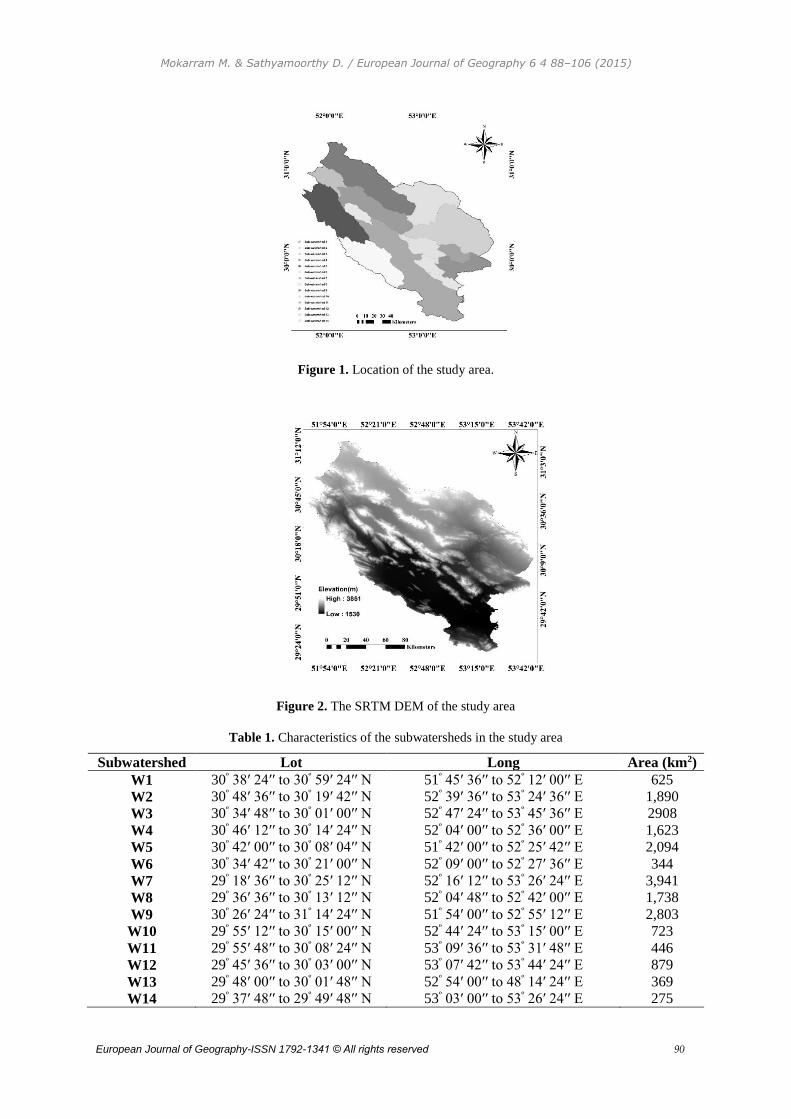
Mokarram M. & Sathyamoorthy D. / European Journal of Geography 6 4 88–106 (2015)
European Journal of Geography-ISSN 1792-1341 © All rights reserved 90
Figure 1. Location of the study area.
Figure 2. The SRTM DEM of the study area
Table 1. Characteristics of the subwatersheds in the study area
Subwatershed Lot Long Area (km2)
W1 30º 38′ 24′′ to 30º 59′ 24′′ N 51º 45′ 36′′ to 52º 12′ 00′′ E 625
W2 30º 48′ 36′′ to 30º 19′ 42′′ N 52º 39′ 36′′ to 53º 24′ 36′′ E 1,890
W3 30º 34′ 48′′ to 30º 01′ 00′′ N 52º 47′ 24′′ to 53º 45′ 36′′ E 2908
W4 30º 46′ 12′′ to 30º 14′ 24′′ N 52º 04′ 00′′ to 52º 36′ 00′′ E 1,623
W5 30º 42′ 00′′ to 30º 08′ 04′′ N 51º 42′ 00′′ to 52º 25′ 42′′ E 2,094
W6 30º 34′ 42′′ to 30º 21′ 00′′ N 52º 09′ 00′′ to 52º 27′ 36′′ E 344
W7 29º 18′ 36′′ to 30º 25′ 12′′ N 52º 16′ 12′′ to 53º 26′ 24′′ E 3,941
W8 29º 36′ 36′′ to 30º 13′ 12′′ N 52º 04′ 48′′ to 52º 42′ 00′′ E 1,738
W9 30º 26′ 24′′ to 31º 14′ 24′′ N 51º 54′ 00′′ to 52º 55′ 12′′ E 2,803
W10 29º 55′ 12′′ to 30º 15′ 00′′ N 52º 44′ 24′′ to 53º 15′ 00′′ E 723
W11 29º 55′ 48′′ to 30º 08′ 24′′ N 53º 09′ 36′′ to 53º 31′ 48′′ E 446
W12 29º 45′ 36′′ to 30º 03′ 00′′ N 53º 07′ 42′′ to 53º 44′ 24′′ E 879
W13 29º 48′ 00′′ to 30º 01′ 48′′ N 52º 54′ 00′′ to 48º 14′ 24′′ E 369
W14 29º 37′ 48′′ to 29º 49′ 48′′ N 53º 03′ 00′′ to 53º 26′ 24′′ E 275
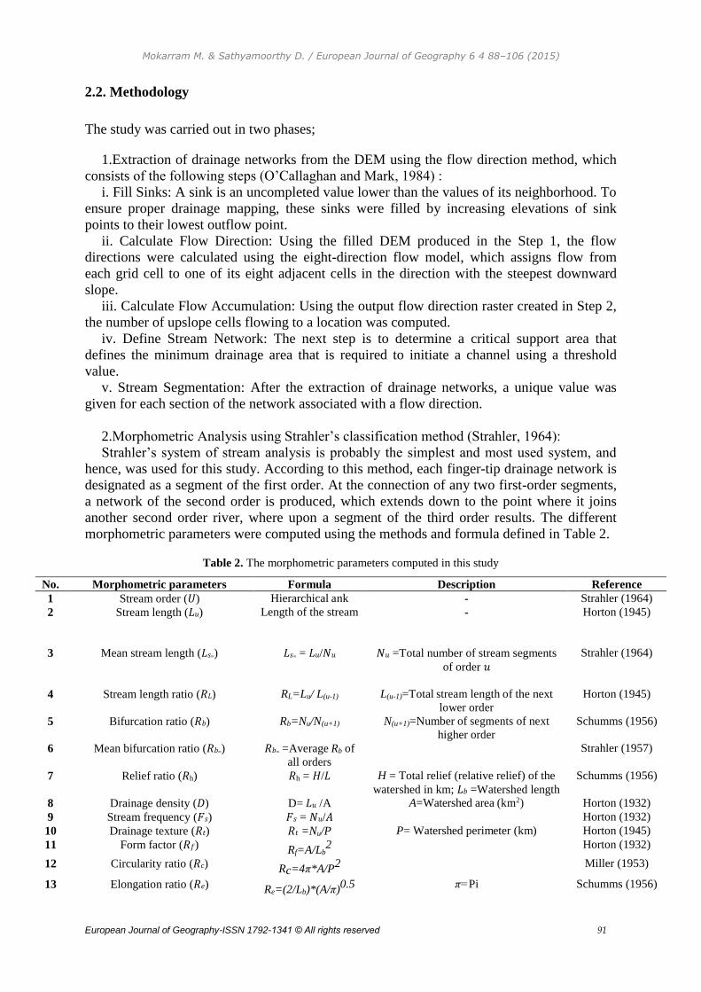
Mokarram M. & Sathyamoorthy D. / European Journal of Geography 6 4 88–106 (2015)
European Journal of Geography-ISSN 1792-1341 © All rights reserved 91
2.2. Methodology
The study was carried out in two phases;
1.Extraction of drainage networks from the DEM using the flow direction method, which
consists of the following steps (O’Callaghan and Mark, 1984) :
i. Fill Sinks: A sink is an uncompleted value lower than the values of its neighborhood. To
ensure proper drainage mapping, these sinks were filled by increasing elevations of sink
points to their lowest outflow point.
ii. Calculate Flow Direction: Using the filled DEM produced in the Step 1, the flow
directions were calculated using the eight-direction flow model, which assigns flow from
each grid cell to one of its eight adjacent cells in the direction with the steepest downward
slope.
iii. Calculate Flow Accumulation: Using the output flow direction raster created in Step 2,
the number of upslope cells flowing to a location was computed.
iv. Define Stream Network: The next step is to determine a critical support area that
defines the minimum drainage area that is required to initiate a channel using a threshold
value.
v. Stream Segmentation: After the extraction of drainage networks, a unique value was
given for each section of the network associated with a flow direction.
2.Morphometric Analysis using Strahler’s classification method (Strahler, 1964):
Strahler’s system of stream analysis is probably the simplest and most used system, and
hence, was used for this study. According to this method, each finger-tip drainage network is
designated as a segment of the first order. At the connection of any two first-order segments,
a network of the second order is produced, which extends down to the point where it joins
another second order river, where upon a segment of the third order results. The different
morphometric parameters were computed using the methods and formula defined in Table 2.
Table 2. The morphometric parameters computed in this study
No. Morphometric parameters Formula Description Reference
1 Stream order (𝑈) Hierarchical ank - Strahler (1964)
2 Stream length (𝐿𝑢) Length of the stream
- Horton (1945)
3 Mean stream length (𝐿𝑠𝑚) 𝐿𝑠𝑚 = 𝐿𝑢/𝑁𝑢 𝑁𝑢 =Total number of stream segments
of order 𝑢
Strahler (1964)
4 Stream length ratio (𝑅𝐿) RL=Lu/ L(u-1) L(u-1)=Total stream length of the next
lower order
Horton (1945)
5 Bifurcation ratio (𝑅𝑏) Rb=Nu/N(u+1) N(u+1)=Number of segments of next
higher order
Schumms (1956)
6 Mean bifurcation ratio (𝑅𝑏𝑚) 𝑅𝑏𝑚 =Average Rb of
all orders
Strahler (1957)
7 Relief ratio (𝑅h) 𝑅h = 𝐻/𝐿 H = Total relief (relative relief) of the
watershed in km; 𝐿𝑏 =Watershed length
Schumms (1956)
8 Drainage density (𝐷) D= 𝐿𝑢 /A A=Watershed area (km2) Horton (1932)
9 Stream frequency (𝐹𝑠) 𝐹𝑠 = 𝑁𝑢/𝐴 Horton (1932)
10 Drainage texture (𝑅𝑡) 𝑅𝑡 =Nu/P P= Watershed perimeter (km) Horton (1945)
11 Form factor (𝑅𝑓) Rf=A/Lb2
Horton (1932)
12 Circularity ratio (𝑅𝑐) Rc=4π*A/P2
Miller (1953)
13 Elongation ratio (𝑅𝑒) Re=(2/Lb)*(A/π)0.5
π=Pi Schumms (1956)

Mokarram M. & Sathyamoorthy D. / European Journal of Geography 6 4 88–106 (2015)
European Journal of Geography-ISSN 1792-1341 © All rights reserved 92
14 Length of overland flow (𝐿𝑔) 𝐿𝑔 =1/D*2 Horton (1945)
15 Constant channel maintenance (𝐶) 𝐶=1/𝐷 Schumms (1956)
16 Shape index (𝑆𝑤) 𝑆𝑤 = 𝐿𝑏/𝐴 Horton (1945)
17 Ruggedness number (𝑅𝑛) 𝑅𝑛 = 𝐵h*𝐷 𝐵h = Watershed relief; D = Drainage
density
Pareta and Pareta
(2011)
18 Shape factor (𝑅𝑠) 𝑅𝑠 = 𝑃𝑢/𝑃𝑐
Where 𝑃𝑢 = Perimeter of circle of
watershed area; 𝑃𝑐 = Perimeter of
watershed
Sameena et al.
(2009)
19 Compactness coefficient (𝐶𝑐) Cc= 0.2821P/A 0.5
Suresh et al.
(2004)
Finally, MLR was used to determine the correlation between the morphometric parameters.
The general purpose of multiple regressions is to learn more about the relationship between
several independent or predictor variables, and a dependent or criterion variable. The general
form of the regression equations is:
Y=A0 + A1X1 + A2X2 + … + bnXn
(1)
where Y is the dependent variable, A0 is the intercept, A1 and bn are regression coefficients,
and X1– Xn are independent variables referring to basic soil properties.
3. RESULTS
The extracted drainage networks for the subwatersheds are shown in Figure 3. Minimum
elevation, maximum elevation, relative relief, and subwatershed area (A), perimeter (P) and
length, which are important parameters in quantitative morphology, were computed for each
subwatershed (Table 3). Subwatershed area is hydrologically important because it directly
affects the size of the magnitudes of peak and mean runoff, whereby the maximum flood
discharge per unit area is inversely related to size (Chorley et al., 1957).
(1) (2)
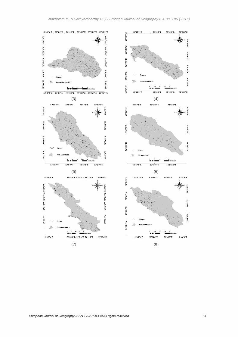
Mokarram M. & Sathyamoorthy D. / European Journal of Geography 6 4 88–106 (2015)
European Journal of Geography-ISSN 1792-1341 © All rights reserved 93
(3) (4)
(5) (6)
(7) (8)
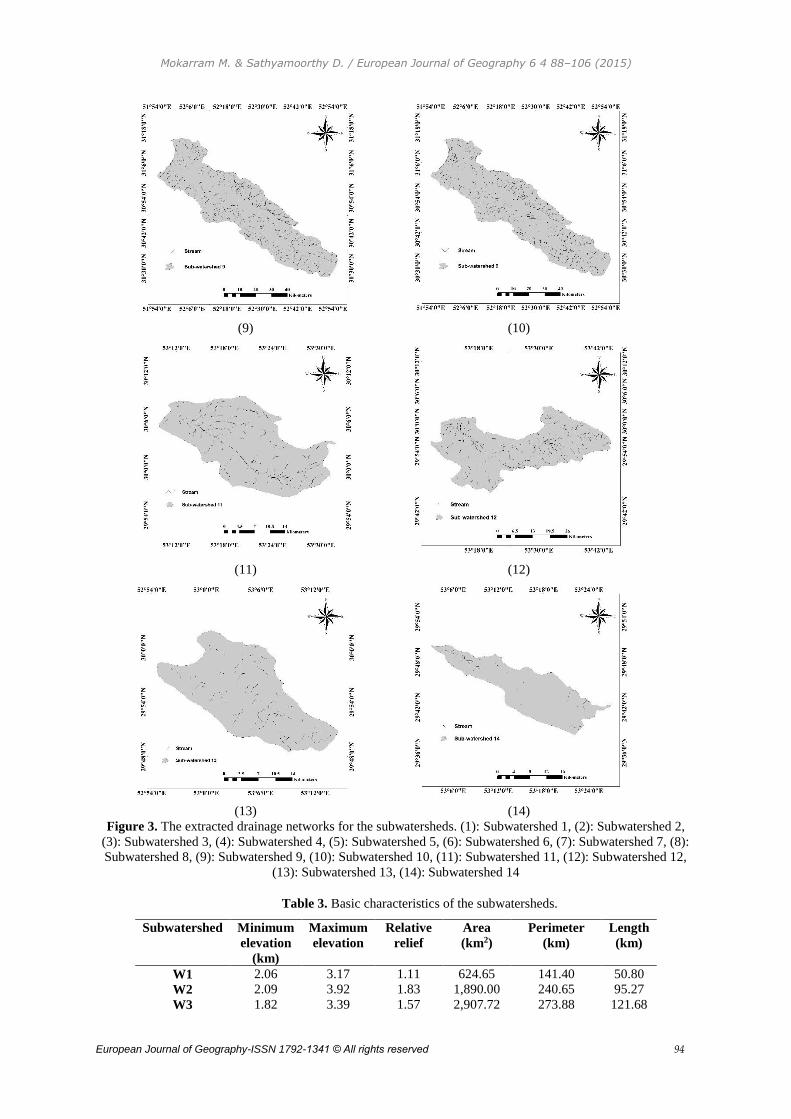
Mokarram M. & Sathyamoorthy D. / European Journal of Geography 6 4 88–106 (2015)
European Journal of Geography-ISSN 1792-1341 © All rights reserved 94
(9) (10)
(11) (12)
(13) (14)
Figure 3. The extracted drainage networks for the subwatersheds. (1): Subwatershed 1, (2): Subwatershed 2,
(3): Subwatershed 3, (4): Subwatershed 4, (5): Subwatershed 5, (6): Subwatershed 6, (7): Subwatershed 7, (8):
Subwatershed 8, (9): Subwatershed 9, (10): Subwatershed 10, (11): Subwatershed 11, (12): Subwatershed 12,
(13): Subwatershed 13, (14): Subwatershed 14
Table 3. Basic characteristics of the subwatersheds.
Subwatershed Minimum
elevation
(km)
Maximum
elevation
Relative
relief
Area
(km2)
Perimeter
(km)
Length
(km)
W1 2.06 3.17 1.11 624.65 141.40 50.80
W2 2.09 3.92 1.83 1,890.00 240.65 95.27
W3 1.82 3.39 1.57 2,907.72 273.88 121.68

Mokarram M. & Sathyamoorthy D. / European Journal of Geography 6 4 88–106 (2015)
European Journal of Geography-ISSN 1792-1341 © All rights reserved 95
W4 2.06 3.50 1.44 1,623.08 240.56 87.38
W5 1.63 3.71 2.08 2,094.42 255.73 100.99
W6 2.15 3.13 0.98 343.67 90.08 36.18
W7 1.54 3.10 1.56 3941.44 475.14 144.63
W8 1.57 2.89 1.32 1,737.63 229.99 90.83
W9 2.29 3.48 1.19 2,803.31 318.82 119.18
W10 1.66 3.13 1.47 723.30 152.48 55.21
W11 1.80 2.56 0.76 446.31 104.08 41.97
W12 1.57 3.25 1.68 878.72 178.33 61.67
W13 1.60 2.83 1.23 369.19 93.80 37.68
W14 1.53 2.52 0.99 275.21 100.08 31.89
The highest stream order among the 14 subwatersheds is 4, which is shown by seven
subwatersheds; W2, W5, W7, W8, W9, W11 and W12. The lowest stream order is 3, which
is shown by the remaining subwatersheds; W1, W3, W4, W6, W10, W13 and W14. A perusal
of Table 4 indicates that the 14 subwatersheds drain into the north of the Fars province,
contributing surface runoff and sediment loads due to variations in their physical
characteristics. Higher stream order is associated with greater discharge and higher velocity
(Costa, 1987). The west of the study area clearly contributes more discharge and since higher
velocity enhances erosion rates, this side also contributes higher sediment loads into the study
area.
Furthermore, the total number of stream segments decrease with stream order. This is
referred to as Horton’s law of stream numbers. Any deviation indicates that the terrain is
typified with high relief and/or moderately steep slopes, underlain by varying lithology and
probable uplift across the watershed (Singh and Singh, 1997). In practice, when logarithms of
the number of streams of a given order are plotted against the order, the points lie on a
straight line (Horton, 1945). A similar geometric relationship was also found between stream
order and stream numbers for all the subwatersheds (Figure 4). This indicates that the whole
area has uniform underlying lithology, and geologically, there has been no probable uplift in
the watershed.
Table 4. Stream order, stream number and stream length of the subwatersheds.
Sub-
watershed
Stream
order
Stream number Stream length (km)
I II III IV I II III IV
W1 3 184 78 9 - 195.53 72.14 6.27 -
W2 4 518 207 63 3 715.24 202.380 47.04 0.996
W3 3 643 277 80 - 1000.42 411.13 98.693 -
W4 3 395 145 28 - 584.93 174.196 34.173 -
W5 4 457 250 49 13 696.37 234.82 45.565 9.230
W6 3 92 28 1 - 140.599 30.865 0.040 -
W7 4 986 363 81 9 770.733 249.243 60.176 11.972
W8 4 442 178 61 13 316.91 181.067 82.672 6.271
W9 4 704 277 67 6 827.25 326.92 58.35 5.973
W10 3 170 57 12 - 209.108 54.840 7.874 -
W11 4 99 51 8 10 157.231 63.56 9.373 5.672
W12 4 238 93 20 5 317.47 97.727 14.245 2.114
W13 3 85 27 3 - 98.011 23.191 2.414 -
W14 3 90 16 1 - 33.836 9.231 2.251 -
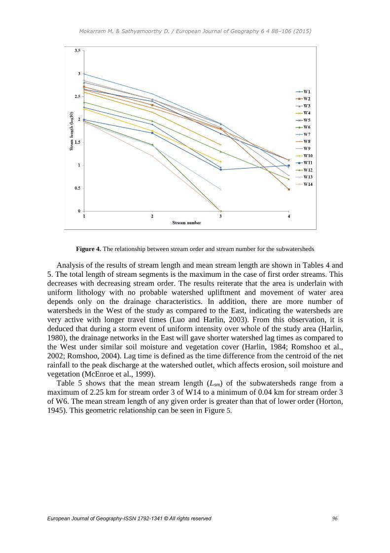
Mokarram M. & Sathyamoorthy D. / European Journal of Geography 6 4 88–106 (2015)
European Journal of Geography-ISSN 1792-1341 © All rights reserved 96
Figure 4. The relationship between stream order and stream number for the subwatersheds
Analysis of the results of stream length and mean stream length are shown in Tables 4 and
5. The total length of stream segments is the maximum in the case of first order streams. This
decreases with decreasing stream order. The results reiterate that the area is underlain with
uniform lithology with no probable watershed upliftment and movement of water area
depends only on the drainage characteristics. In addition, there are more number of
watersheds in the West of the study as compared to the East, indicating the watersheds are
very active with longer travel times (Luo and Harlin, 2003). From this observation, it is
deduced that during a storm event of uniform intensity over whole of the study area (Harlin,
1980), the drainage networks in the East will gave shorter watershed lag times as compared to
the West under similar soil moisture and vegetation cover (Harlin, 1984; Romshoo et al.,
2002; Romshoo, 2004). Lag time is defined as the time difference from the centroid of the net
rainfall to the peak discharge at the watershed outlet, which affects erosion, soil moisture and
vegetation (McEnroe et al., 1999).
Table 5 shows that the mean stream length (Lsm) of the subwatersheds range from a
maximum of 2.25 km for stream order 3 of W14 to a minimum of 0.04 km for stream order 3
of W6. The mean stream length of any given order is greater than that of lower order (Horton,
1945). This geometric relationship can be seen in Figure 5.
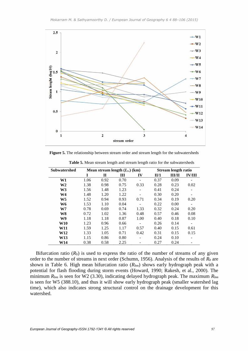
Mokarram M. & Sathyamoorthy D. / European Journal of Geography 6 4 88–106 (2015)
European Journal of Geography-ISSN 1792-1341 © All rights reserved 97
Figure 5. The relationship between stream order and stream length for the subwatersheds
Table 5. Mean stream length and stream length ratio for the subwatersheds
Subwatershed Mean stream length (Lsm) (km) Stream length ratio
I II III IV II/1 III/II IV/III
W1 1.06 0.92 0.70 - 0.37 0.09 -
W2 1.38 0.98 0.75 0.33 0.28 0.23 0.02
W3 1.56 1.48 1.23 - 0.41 0.24 -
W4 1.48 1.20 1.22 - 0.30 0.20 -
W5 1.52 0.94 0.93 0.71 0.34 0.19 0.20
W6 1.53 1.10 0.04 - 0.22 0.00 -
W7 0.78 0.69 0.74 1.33 0.32 0.24 0.20
W8 0.72 1.02 1.36 0.48 0.57 0.46 0.08
W9 1.18 1.18 0.87 1.00 0.40 0.18 0.10
W10 1.23 0.96 0.66 - 0.26 0.14 -
W11 1.59 1.25 1.17 0.57 0.40 0.15 0.61
W12 1.33 1.05 0.71 0.42 0.31 0.15 0.15
W13 1.15 0.86 0.80 - 0.24 0.10 -
W14 0.38 0.58 2.25 - 0.27 0.24 -
Bifurcation ratio (Rb) is used to express the ratio of the number of streams of any given
order to the number of streams in next order (Schumn, 1956). Analysis of the results of Rb are
shown in Table 6. High mean bifurcation ratio (Rbm) shows early hydrograph peak with a
potential for flash flooding during storm events (Howard, 1990; Rakesh, et al., 2000). The
minimum Rbm is seen for W2 (3.30), indicating delayed hydrograph peak. The maximum Rbm
is seen for W5 (388.10), and thus it will show early hydrograph peak (smaller watershed lag
time), which also indicates strong structural control on the drainage development for this
watershed.
Mokarram M. & Sathyamoorthy D. / European Journal of Geography 6 4 88–106 (2015)
European Journal of Geography-ISSN 1792-1341 © All rights reserved 98
Table 6. Bifurcation ratio, drainage density and stream frequency of the subwatersheds
Subwatershed Bifurcation ratio (Rb) Mean
bifurcation
ratio (Rbm)
Drainage
density
(D)
Stream
frequency
(Fs)
I/II II/III III/IV
W1 2.71 11.51 - 7.11 0.44 0.43
W2 3.53 4.30 47.23 18.35 0.51 0.42
W3 2.43 4.17 - 3.30 0.52 0.34
W4 3.36 5.10 - 4.23 0.49 0.35
W5 2.97 5.15 4.94 4.35 0.47 0.37
W6 4.56 771.63 - 388.10 0.50 0.35
W7 3.09 4.14 5.03 4.09 0.28 0.37
W8 1.75 2.19 13.18 5.71 0.34 0.40
W9 2.53 5.60 9.77 5.97 0.43 0.38
W10 3.81 6.96 - 5.39 0.38 0.33
W11 2.47 6.78 1.65 3.63 0.53 0.38
W12 3.25 6.86 6.74 5.62 0.49 0.41
W13 4.23 9.61 - 6.92 0.33 0.31
W14 3.67 4.10 - 3.89 0.16 0.39
The travel time by water within the watershed is controlled by drainage density (D) (Gardiner
and Park, 1978; Dodov and Foufoula-Georgiou, 2006). Generally, D varies between 0.55 and
2.09 km/km2. High values of D are observed in regions of weak and impermeable subsurface
material, sparse vegetation, and mountainous relief. On the other hand, regions with low
values of D are underlain with highly resistant permeable material with dense vegetative
cover and low relief. Table 6 indicates that all the watersheds have low values of D (below
2.0 km/km2). This indicates that they are composed of permeable subsurface material, good
vegetation cover and low relief, which results in more infiltration capacity and are good sites
for ground water recharge as compared to watersheds with high values of high D.
Stream frequency (Fs) is the total number of streams of all orders per unit area. The low
values of Fs for all the subwatersheds indicate that the study area is comparably covered with
a good amount of vegetation and has very good infiltration capacity. Overall, the discharge
from all the subwatersheds takes long time to peak because of low runoff rates due to lesser
number of streams (Patton and Baker, 1976; Montgomery and Dietrich, 1989; Montgomery
and Dietrich, 1992; Ghoneim et al., 2002).
Drainage texture (Rt) is influenced by infiltration capacity (Horton, 1945). There are five
different texture classes: very coarse (<2), coarse (2–4), moderate (4–6), fine (6–8), and very
fine (>8) (Smith, 1950). According to this classification, W1, W6, W10, W11, W13 and W14
have very coarse drainage texture, while W2, W3, W4, W5, W7, W8, W9 and W12 have
coarse drainage texture (Table 7). Hydrologically, very coarse texture subwatersheds have
large watershed lag time periods (Esper Angillieri, 2008) followed by coarse, fine, and very
fine texture classes. This indicates that W1, W6, W10, W11, W13 and W14 (Rt <2) have
longer durations to peak flow, while the other subwatersheds (2<Rt<4) have shorter durations
to peak flow.
Mokarram M. & Sathyamoorthy D. / European Journal of Geography 6 4 88–106 (2015)
European Journal of Geography-ISSN 1792-1341 © All rights reserved 99
Table 7. Drainage texture, constant channel maintenance, shape index, ruggedness number and shape factor of
the subwatersheds
Subwatershed Drainage
texture
(𝑅𝑡)
Constant
channel
maintenance (𝐶)
Compactness
coefficient
(𝐶𝑐)
Shape
index (𝑆𝑤)
Ruggedness
number (𝑅𝑛)
Shape
factor (𝑅𝑠)
W1 1.92 2.27 1.60 4.13 0.49 0.18
W2 3.29 1.96 1.56 4.80 0.93 0.18
W3 3.65 1.92 1.43 5.09 0.82 0.20
W4 2.36 2.04 1.68 4.70 0.71 0.17
W5 3.01 2.13 1.58 4.87 0.98 0.18
W6 1.34 2.00 1.37 3.81 0.49 0.21
W7 3.03 3.57 2.13 5.31 0.44 0.13
W8 3.02 2.94 1.56 4.75 0.45 0.18
W9 3.31 2.33 1.70 5.07 0.51 0.17
W10 1.57 2.63 1.60 4.21 0.56 0.18
W11 1.61 1.89 1.39 3.95 0.40 0.20
W12 2.00 2.04 1.70 4.33 0.82 0.17
W13 1.23 3.03 1.38 3.85 0.41 0.20
W14 1.07 6.25 1.70 3.70 0.16 0.17
The minimum and maximum shape factors (Rs) are for W7 and W6 respectively, as shown
in Table 7. This parameter is similar in interpretation to circularity ratio, elongation ratio and
form factor (Tucker and Bras, 1998). It gives an idea about the circular character of the
subwatershed. The greater the circular character of the subwatershed, the greater is the rapid
response of the subwatershed after a storm event (Tucker and Bras, 1998). Therefore, in
terms of only Rs, W7 has the longest watershed lag time.
The ruggedness number (Rn) shows the structural complexity of the terrain in association
with relief and drainage density. High values of Rn imply that the area is susceptible to soil
erosion (Rashid et al., 2011; Zaz and Romshoo, 2012). In the present study, Rn is minimum in
case of W14 (0.16) and maximum for W5 (0.98), as seen in Table 7.
Shape index (Sw) shows the rate of water and sediment yield along the length and relief of
the subwatersheds. The shape index values for the subwatersheds of the study area range
from 3.70 for W14 to 5.31 for W7 as shown in Table 7. In terms of only Sw, WS7 will have
the shortest watershed lag time, while WS14 will have the longest watershed lag time.
The relationship of a subwatershed with that of a circular subwatershed having the same
area is shown by the compactness coefficient (Cc). A circular subwatershed yields the
shortest time of concentration before peak flow occurs in the subwatersed. Cc = 1 indicates
that the subwatershed completely behaves as a circular subwatershed. Cc > 1 indicates more
deviation from the circular nature of the subwatershed. The values for all the subwatersheds
range from 1.37 for W6 to 2.13 for W7, as seen in Table 7. Consequently, WS6 has the
greatest deviation from the circular nature, and on the basis of this parameter alone, it will
have the longest time of concentration before peak flow occurs as compared to the other
subwatersheds (Potter and Faulkner, 1987; Tucker and Bras, 1998).
Constant channel maintenance (C) varies from 1.89 for W11 to 6.25 for W14 as is shown
in Table 7. Low values of � for W11 and W9 show that among the 14 subwatersheds, these
two are associated with the weakest or very low-resistance soils, sparse vegetation and
mountainous terrain, while watershed W14 is associated with high-resistance soils, vegetation
and comparably plain terrain (Shulits, 1968).
Relief ratio (Rh) is an indicator of the intensity of erosion processes operating on the
subwatershed slopes (Dodov and Foufoula-Georgiou, 2005). Rh normally increases with
decreasing drainage area and size of a given subwatershed (Gottschalk, 1964). In the study
area, according to in Table 8, Rh ranges from a minimum of 0.01, for W3, W7, W8 and W9,
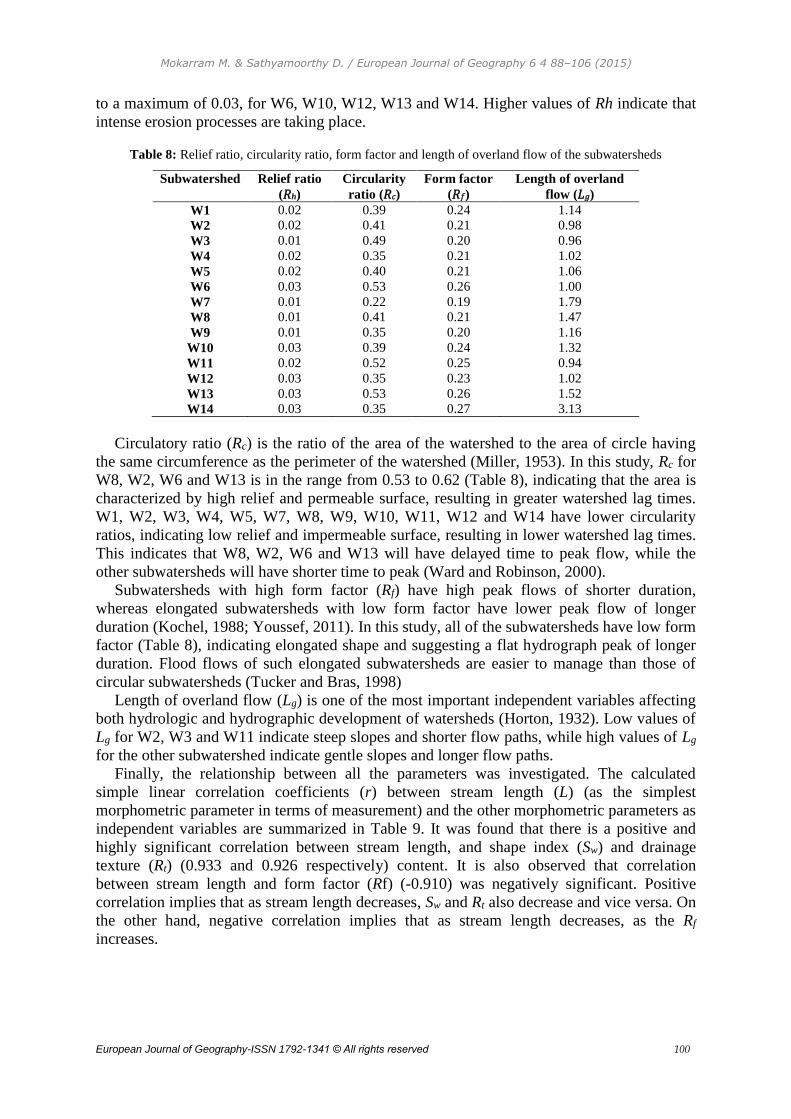
Mokarram M. & Sathyamoorthy D. / European Journal of Geography 6 4 88–106 (2015)
European Journal of Geography-ISSN 1792-1341 © All rights reserved 100
to a maximum of 0.03, for W6, W10, W12, W13 and W14. Higher values of Rh indicate that
intense erosion processes are taking place.
Table 8: Relief ratio, circularity ratio, form factor and length of overland flow of the subwatersheds
Subwatershed Relief ratio
(𝑅h)
Circularity
ratio (𝑅𝑐)
Form factor
(𝑅𝑓)
Length of overland
flow (𝐿𝑔) W1 0.02 0.39 0.24 1.14
W2 0.02 0.41 0.21 0.98
W3 0.01 0.49 0.20 0.96
W4 0.02 0.35 0.21 1.02
W5 0.02 0.40 0.21 1.06
W6 0.03 0.53 0.26 1.00
W7 0.01 0.22 0.19 1.79
W8 0.01 0.41 0.21 1.47
W9 0.01 0.35 0.20 1.16
W10 0.03 0.39 0.24 1.32
W11 0.02 0.52 0.25 0.94
W12 0.03 0.35 0.23 1.02
W13 0.03 0.53 0.26 1.52
W14 0.03 0.35 0.27 3.13
Circulatory ratio (Rc) is the ratio of the area of the watershed to the area of circle having
the same circumference as the perimeter of the watershed (Miller, 1953). In this study, Rc for
W8, W2, W6 and W13 is in the range from 0.53 to 0.62 (Table 8), indicating that the area is
characterized by high relief and permeable surface, resulting in greater watershed lag times.
W1, W2, W3, W4, W5, W7, W8, W9, W10, W11, W12 and W14 have lower circularity
ratios, indicating low relief and impermeable surface, resulting in lower watershed lag times.
This indicates that W8, W2, W6 and W13 will have delayed time to peak flow, while the
other subwatersheds will have shorter time to peak (Ward and Robinson, 2000).
Subwatersheds with high form factor (Rf) have high peak flows of shorter duration,
whereas elongated subwatersheds with low form factor have lower peak flow of longer
duration (Kochel, 1988; Youssef, 2011). In this study, all of the subwatersheds have low form
factor (Table 8), indicating elongated shape and suggesting a flat hydrograph peak of longer
duration. Flood flows of such elongated subwatersheds are easier to manage than those of
circular subwatersheds (Tucker and Bras, 1998)
Length of overland flow (Lg) is one of the most important independent variables affecting
both hydrologic and hydrographic development of watersheds (Horton, 1932). Low values of
Lg for W2, W3 and W11 indicate steep slopes and shorter flow paths, while high values of Lg
for the other subwatershed indicate gentle slopes and longer flow paths.
Finally, the relationship between all the parameters was investigated. The calculated
simple linear correlation coefficients (r) between stream length (L) (as the simplest
morphometric parameter in terms of measurement) and the other morphometric parameters as
independent variables are summarized in Table 9. It was found that there is a positive and
highly significant correlation between stream length, and shape index (Sw) and drainage
texture (Rt) (0.933 and 0.926 respectively) content. It is also observed that correlation
between stream length and form factor (Rf) (-0.910) was negatively significant. Positive
correlation implies that as stream length decreases, Sw and Rt also decrease and vice versa. On
the other hand, negative correlation implies that as stream length decreases, as the Rf
increases.
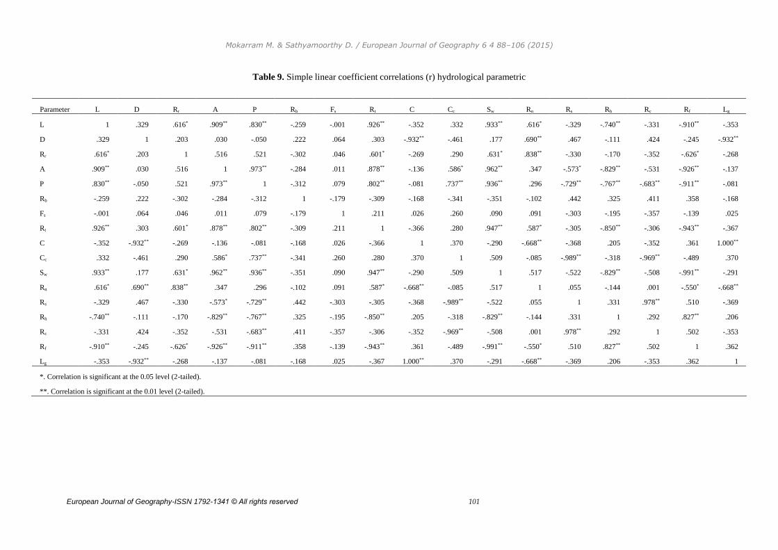
Mokarram M. & Sathyamoorthy D. / European Journal of Geography 6 4 88–106 (2015)
European Journal of Geography-ISSN 1792-1341 © All rights reserved 101
Table 9. Simple linear coefficient correlations (r) hydrological parametric
Parameter L D Rr A P Rb Fs Rt C Cc Sw Rn Rs Rh Rc Rf Lg
L 1 .329 .616* .909** .830** -.259 -.001 .926** -.352 .332 .933** .616* -.329 -.740** -.331 -.910** -.353
D .329 1 .203 .030 -.050 .222 .064 .303 -.932** -.461 .177 .690** .467 -.111 .424 -.245 -.932**
Rr .616* .203 1 .516 .521 -.302 .046 .601* -.269 .290 .631* .838** -.330 -.170 -.352 -.626* -.268
A .909** .030 .516 1 .973** -.284 .011 .878** -.136 .586* .962** .347 -.573* -.829** -.531 -.926** -.137
P .830** -.050 .521 .973** 1 -.312 .079 .802** -.081 .737** .936** .296 -.729** -.767** -.683** -.911** -.081
Rb -.259 .222 -.302 -.284 -.312 1 -.179 -.309 -.168 -.341 -.351 -.102 .442 .325 .411 .358 -.168
Fs -.001 .064 .046 .011 .079 -.179 1 .211 .026 .260 .090 .091 -.303 -.195 -.357 -.139 .025
Rt .926** .303 .601* .878** .802** -.309 .211 1 -.366 .280 .947** .587* -.305 -.850** -.306 -.943** -.367
C -.352 -.932** -.269 -.136 -.081 -.168 .026 -.366 1 .370 -.290 -.668** -.368 .205 -.352 .361 1.000**
Cc .332 -.461 .290 .586* .737** -.341 .260 .280 .370 1 .509 -.085 -.989** -.318 -.969** -.489 .370
Sw .933** .177 .631* .962** .936** -.351 .090 .947** -.290 .509 1 .517 -.522 -.829** -.508 -.991** -.291
Rn .616* .690** .838** .347 .296 -.102 .091 .587* -.668** -.085 .517 1 .055 -.144 .001 -.550* -.668**
Rs -.329 .467 -.330 -.573* -.729** .442 -.303 -.305 -.368 -.989** -.522 .055 1 .331 .978** .510 -.369
Rh -.740** -.111 -.170 -.829** -.767** .325 -.195 -.850** .205 -.318 -.829** -.144 .331 1 .292 .827** .206
Rc -.331 .424 -.352 -.531 -.683** .411 -.357 -.306 -.352 -.969** -.508 .001 .978** .292 1 .502 -.353
Rf -.910** -.245 -.626* -.926** -.911** .358 -.139 -.943** .361 -.489 -.991** -.550* .510 .827** .502 1 .362
Lg -.353 -.932** -.268 -.137 -.081 -.168 .025 -.367 1.000** .370 -.291 -.668** -.369 .206 -.353 .362 1
*. Correlation is significant at the 0.05 level (2-tailed).
**. Correlation is significant at the 0.01 level (2-tailed).
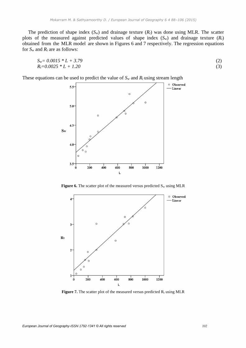
Mokarram M. & Sathyamoorthy D. / European Journal of Geography 6 4 88–106 (2015)
European Journal of Geography-ISSN 1792-1341 © All rights reserved 102
The prediction of shape index (Sw) and drainage texture (Rt) was done using MLR. The scatter
plots of the measured against predicted values of shape index (Sw) and drainage texture (Rt)
obtained from the MLR model are shown in Figures 6 and 7 respectively. The regression equations
for Sw and Rt are as follows:
Sw= 0.0015 * L + 3.79 (2)
Rt=0.0025 * L + 1.20 (3)
These equations can be used to predict the value of Sw and Rt using stream length
Figure 6. The scatter plot of the measured versus predicted Sw using MLR
Figure 7. The scatter plot of the measured versus predicted Rt using MLR
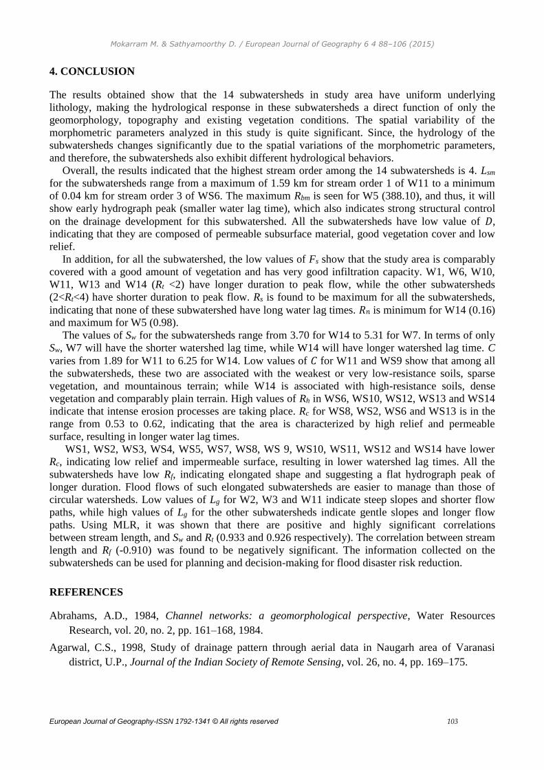
Mokarram M. & Sathyamoorthy D. / European Journal of Geography 6 4 88–106 (2015)
European Journal of Geography-ISSN 1792-1341 © All rights reserved 103
4. CONCLUSION
The results obtained show that the 14 subwatersheds in study area have uniform underlying
lithology, making the hydrological response in these subwatersheds a direct function of only the
geomorphology, topography and existing vegetation conditions. The spatial variability of the
morphometric parameters analyzed in this study is quite significant. Since, the hydrology of the
subwatersheds changes significantly due to the spatial variations of the morphometric parameters,
and therefore, the subwatersheds also exhibit different hydrological behaviors.
Overall, the results indicated that the highest stream order among the 14 subwatersheds is 4. Lsm
for the subwatersheds range from a maximum of 1.59 km for stream order 1 of W11 to a minimum
of 0.04 km for stream order 3 of WS6. The maximum Rbm is seen for W5 (388.10), and thus, it will
show early hydrograph peak (smaller water lag time), which also indicates strong structural control
on the drainage development for this subwatershed. All the subwatersheds have low value of 𝐷,
indicating that they are composed of permeable subsurface material, good vegetation cover and low
relief.
In addition, for all the subwatershed, the low values of Fs show that the study area is comparably
covered with a good amount of vegetation and has very good infiltration capacity. W1, W6, W10,
W11, W13 and W14 (Rt <2) have longer duration to peak flow, while the other subwatersheds
(2<Rt<4) have shorter duration to peak flow. Rs is found to be maximum for all the subwatersheds,
indicating that none of these subwatershed have long water lag times. 𝑅𝑛 is minimum for W14 (0.16)
and maximum for W5 (0.98).
The values of Sw for the subwatersheds range from 3.70 for W14 to 5.31 for W7. In terms of only
Sw, W7 will have the shorter watershed lag time, while W14 will have longer watershed lag time. C
varies from 1.89 for W11 to 6.25 for W14. Low values of 𝐶 for W11 and WS9 show that among all
the subwatersheds, these two are associated with the weakest or very low-resistance soils, sparse
vegetation, and mountainous terrain; while W14 is associated with high-resistance soils, dense
vegetation and comparably plain terrain. High values of Rh in WS6, WS10, WS12, WS13 and WS14
indicate that intense erosion processes are taking place. Rc for WS8, WS2, WS6 and WS13 is in the
range from 0.53 to 0.62, indicating that the area is characterized by high relief and permeable
surface, resulting in longer water lag times.
WS1, WS2, WS3, WS4, WS5, WS7, WS8, WS 9, WS10, WS11, WS12 and WS14 have lower
Rc, indicating low relief and impermeable surface, resulting in lower watershed lag times. All the
subwatersheds have low Rf, indicating elongated shape and suggesting a flat hydrograph peak of
longer duration. Flood flows of such elongated subwatersheds are easier to manage than those of
circular watersheds. Low values of Lg for W2, W3 and W11 indicate steep slopes and shorter flow
paths, while high values of Lg for the other subwatersheds indicate gentle slopes and longer flow
paths. Using MLR, it was shown that there are positive and highly significant correlations
between stream length, and Sw and Rt (0.933 and 0.926 respectively). The correlation between stream
length and Rf (-0.910) was found to be negatively significant. The information collected on the
subwatersheds can be used for planning and decision-making for flood disaster risk reduction.
REFERENCES
Abrahams, A.D., 1984, Channel networks: a geomorphological perspective, Water Resources
Research, vol. 20, no. 2, pp. 161–168, 1984.
Agarwal, C.S., 1998, Study of drainage pattern through aerial data in Naugarh area of Varanasi
district, U.P., Journal of the Indian Society of Remote Sensing, vol. 26, no. 4, pp. 169–175.
Mokarram M. & Sathyamoorthy D. / European Journal of Geography 6 4 88–106 (2015)
European Journal of Geography-ISSN 1792-1341 © All rights reserved 104
Akram F., Rasul M.G, Khan M., Amir, M., 2012, Automatic Delineation of Drainage Networks and
Catchments using DEM data and GIS Capabilities: A case study, 18th Australian Fluid
Mechanics Conference, Launceston, Australia.
Altaf, F., Meraj, G., Romshoo, S.A., 2013, Morphometric Analysis to Infer Hydrological Behaviour
of Lidder Watershed, Western Himalaya, India. Hindawi Publishing Corporation Geography
Journal Volume 2013, Article ID 178021, 14 pages
Chorley R.J., Malm D.E.G., Pogorzelki H.A., 1957, A new standard for estimating drainage basin
shape. Am. J. Sci., 255: 138–141.
Costa, J.E., 1987, Hydraulics and basin morphometry of the largest flash floods in the conterminous
United States, Journal of Hydrology, vol. 93, no. 3-4, pp. 313–338.
Dar, R.A., Chandra, R., Romshoo, S.A., 2013, Morphotectonic and lithostratigraphic analysis of
intermontane Karewa basin of Kashmir Himalayas, India, Journal of Mountain Science, vol. 10,
no. 1, pp. 731–741.
Dodov B.A., Foufoula-Georgiou, E., 2006, Floodplain morphom- etry extraction from a high-
resolution digital elevation model: a simple algorithm for regional analysis studies, IEEE
Geoscience and Remote Sensing Letters, vol. 3, no. 3, pp. 410–413.
Dodov, B., Foufoula-Georgiou, E., 2005, Fluvial processes and streamflow variability: interplay in
the scale-frequency contin- uum and implications for scaling, Water Resources Research, vol.
41, no. 5, pp. 1–18.
Esper Angillieri, M.Y., 2008, Morphometric analysis of Colangu il river basin and flash flood
hazard, San Juan, Argentina, Environmental Geology, vol. 55, no. 1, pp. 107–111.
Gardiner, V., Park, C. C., 1978, Drainage basin morphometry,Progress in Physical Geography, vol.
2, no. 1, pp. 1–35.
Gardiner, V., Park, C. C., 1978, Drainage basin morphometry,Progress in Physical Geography, vol.
2, no. 1, pp. 1–35.
Gottschalk, L.C., 1964, Reservoir sedimentation, in Handbook of Applied Hydrology, Chow, V.T.
Ed., section 7-1, McGraw-Hill, New York, NY, USA.
Grohmann, C.H. 2004, Morphometric analysis in Geographic Information Systems: applications of
free software ,GRASS and R. Computers & Geosciences, 30 (9-10):1055-1067.
Harlin, J.M., 1980, The effect of precipitation variability on drainage basin morphometry, American
Journal of Science, vol. 280, no. 8, pp. 812–825.
Harlin, J.M., 1984, Watershed morphometry and time to hydrograph peak, Journal of Hydrology,
vol. 67, no. 1-4, pp. 141–154.
Horton, R.E., 1932, Drainage basin characteristics, Transactions American Geophysical Union, vol.
13, pp. 350–361.
Horton, R.E., 1945, Erosional development of streams and their drainage basins: hydrophysical
approach to quantitative mor- phology, Geological Society of America Bulletin, vol. 56, pp.
275–370.
Howard, A. D., 1990, Role of hypsometry and planform in basin hydrologic response, Hydrological
Processes, vol. 4, no. 4, pp. 373–385.
Mokarram M. & Sathyamoorthy D. / European Journal of Geography 6 4 88–106 (2015)
European Journal of Geography-ISSN 1792-1341 © All rights reserved 105
Kochel, R. C., 1988, Geomorphic impact of large floods: review and new perspectives on magnitude
and frequency, in Flood Geomorphology, pp. 169–187, John Wiley & Sons, New York, NY,
USA.
Leopold, L.B., Maddock, T., 1953, The hydraulic geometry of stream channels and some
physiographic implications, USGS Professional Paper, vol. 252, pp. 1–57.
Luo, W., Harlin, J.M., 2003, A theoretical travel time based on watershed hypsometry, Journal of the
American Water Resources Association, vol. 39, no. 4, pp. 785–792.
Magesh, N.S., Chandrasekar, N., Soundranayagam J.P., 2011, Morphometric evaluation of
Papanasam and Manimuthar watersheds, parts of Western Ghats, Tirunelveli district, Tamil
Nadu, India: a GIS approach. Environ Earth Sci 64:373–381
McEnroe, B.M., Zhao, H., 1999, Lag times and peak coefficients for rural watersheds in kansas.
University of Kansas, Lawrence, Kansas. Report No. K-TRAN: KU-98-1.
Melelli, L., Liucci, L., Vergari, F., Ciccacci, S., Monte, M.D., 2014, Fluvial drainage networks: the
fractal approach as an improvement of quantitative geomorphic analyses. Geophysical Research
Abstracts. Vol. 16, EGU2014-12452.
Mesa, L.M., 2006, Morphometric analysis of a subtropical Andean basin (Tucuman, Argentina).
Environ Geol 50(8):1235–1242
Miller, V.C., 1953, A Quantitative geomorphic study of drainage basin characteristics in the Clinch
Mountain area, Virginia and Tennessee, Tech. Rep. 3 NR 389-402, Columbia University,
Department of Geology, ONR, New York, NY, USA, 1953.
Montgomery, D.R., Dietrich, W.E., 1989, Source areas, drainage density, and channel initiation,
Water Resources Research, vol.25, no. 8, pp. 1907–1918.
Montgomery, D.R., Dietrich, W.E., 1992, Channel initiation and the problem of landscape scale,
Science, vol. 255, no. 5046, pp. 826–830.
Nag, S.K., and Chakraborty, S., 2003, Influence of rock types and structures in the development of
drainage network in hard rock area. J Indian Soc Remote Sens 31(1):25–35
Nissar, A., Kuchay, M., Sultan, B., 2013, Automated drainage characterization of dudganga
watershed in western Himalayas. European Scientific Journal December 2013 edition vol.9,
No.35 ISSN: 1857 – 7881 (Print) e - ISSN 1857- 7431
O’Callaghan, J. F., Mark, D.M., 1984, The extraction of drainage networks from digital elevation
data, Computer Vision, Graph- ics, and Image Processing, vol. 28, pp. 323–344.
Pareta, K., Pareta, U., 2011, Quantitative morphometric analysis of a watershed of Yamuna basin,
India using ASTER (DEM) data and GIS, International Journal of Geomatics and Geosciences,
vol. 2, no. 1.
Patton, P.C., Baker, V. R., 1976, Morphometry and floods in small drainage basins subject to diverse
hydrogeomorphic controls, Water Resources Research, vol. 12, no. 5, pp. 941–952.
Pidwirny, M., 2006, The Drainage Basin Concept. Fundamentals of Physical Geography, 2nd
Edition.
Potter, K.W., Faulkner, E.B., 1987, Catchment response time as a predictor of flood quantiles,
Journal of the American Water Resources Association, vol. 23, no. 5, pp. 857–861.
Mokarram M. & Sathyamoorthy D. / European Journal of Geography 6 4 88–106 (2015)
European Journal of Geography-ISSN 1792-1341 © All rights reserved 106
Rakesh, K., Lohani, A.K., Sanjay, K., Chatterjee, C., Nema, R.K., 2000, GIS based morphometric
analysis of Ajay river basin upto Srarath gauging site of South Bihar, Journal of Applied
Hydrology, vol. 14, no. 4, pp. 45–54.
Rashid, M., Lone, M.A., Romshoo, S.A., 2011, Geospatial tools for assessing land degradation in
Budgam district, Kashmir Himalaya, India, Journal of Earth System Science, vol. 120, no. 3, pp.
423–433.
Romshoo, S.A., 2004, Geostatistical analysis of soil moisture mea- surements and remotely sensed
data at different spatial scales, Environmental Geology, vol. 45, no. 3, pp. 339–349, 2004.
Sameena, M., Krishnamurthy, J., Jayaraman, V., Ranganna, G., 2009, Evaluation of drainage
networks developed in hard rock terrain, Geocarto International, vol. 24, no. 5, pp. 397–420.
Schumms, S.A., 1956, Evolution of drainage systems and slopes in Badlands at Perth Amboy, New
Jersey, Bulletin of the Geological Society of America, vol. 67, pp. 597–646.
Shulits, S., 1968, Quantitative formulation of stream and watershed morphology, Bulletin of the
International Association of Scien- tific Hydrology, vol. 3, pp. 201–207.
Singh, S., 1992, Quantitative geomorphology of the drainage basin, in Readings on Remote Sensing
Applications, T. S. Chouhan and K. N. Joshi, Eds., Scientific Publishers, Jodhpur, India.
Singh, S., Singh, M.C., 1997, Morphometric analysis of Kanhar river basin, The National
Geographical Journal of India, vol. 43, no. 1, pp. 31–43, 1997.
Strahler, A., 1957, Quantitative analysis of watershed geomorphol- ogy, Transactions American
Geophysical Union, vol. 38, pp. 913–920.
Strahler, A.N., 1964, Quantitative geomorphology of drainage basins and channel networks, in
Handbook of Applied Hydrology, V. T. Chow, Ed., section 4–11, McGraw-Hill, New York, NY,
USA,1964.
Suresh, M., Sudhakara, S., Tiwari, K.N., Chowdary, V.M., 2004, Prioritization of watersheds using
morphometric parameters and assessment of surface water potential using remote sens- ing,
Journal of the Indian Society of Remote Sensing, vol. 32, no.3.
Tucker, G.E., Bras, R.L. 1998, Hillslope processes, drainage density, and landscape morphology,
Water Resources Research, vol. 34, no. 10, pp. 2751–2764, 1998.
Ward, R.C., Robinson, M., 2000, Principles of Hydrology, McGraw- Hill, Maidenhead, UK, 4th
edition, 2000.
Youssef, A.M., Pradhan, B., Hassan, A.M., 2011, Flash flood risk estimation along the St. Katherine
road, southern Sinai, Egypt using GIS based morphometry and satellite imagery, Environmental
Earth Sciences, vol. 62, no. 3, pp. 611–623, 2011.
Zaz , S., Romshoo, S. A., 2012, Assessing the geoindicators of land degradation in the Kashmir
Himalayan Region, India, Natural Hazards, vol. 64, no. 2, pp. 1219–1245.
.

EUROPEAN JOURNAL OF GEOGRAPHY
Volume 6 • Number 4 December 2015 • ISSN 1792-1341
E u r o p e a n A s s o c i a t i o n o f G e o g r a p h e r s
Related Documents


![European geography[1]](https://static.cupdf.com/doc/110x72/554c8786b4c905df3c8b543f/european-geography1.jpg)