European atmosphere in 2050, a regional air quality and climate perspective under CMIP5 scenarios

Atmos. Chem. Phys., 13, 7451–7471, 2013www.atmos-chem-phys.net/13/7451/2013/doi:10.5194/acp-13-7451-2013© Author(s) 2013. CC Attribution 3.0 License.

EGU Journal Logos (RGB)

Advances in Geosciences

Open A

ccess

Natural Hazards and Earth System

Sciences

Open A

ccess

Annales Geophysicae

Open A

ccessNonlinear Processes

in Geophysics

Open A

ccess

Atmospheric Chemistry

and PhysicsO

pen Access

Atmospheric Chemistry

and Physics

Open A

ccess

Discussions

Atmospheric Measurement

Techniques

Open A

ccess

Atmospheric Measurement

Techniques

Open A

ccess

Discussions

Biogeosciences

Open A

ccess

Open A

ccess

BiogeosciencesDiscussions

Climate of the Past

Open A

ccess

Open A

ccess

Climate of the Past

Discussions

Earth System Dynamics

Open A

ccess

Open A

ccess

Earth System Dynamics

Discussions

GeoscientificInstrumentation

Methods andData Systems

Open A

ccess

GeoscientificInstrumentation

Methods andData Systems

Open A

ccess

Discussions

GeoscientificModel Development

Open A

ccess

Open A

ccess

GeoscientificModel Development

Discussions

Hydrology and Earth System

Sciences

Open A

ccess

Hydrology and Earth System

Sciences

Open A

ccess

Discussions

Ocean Science

Open A

ccess

Open A

ccess

Ocean ScienceDiscussions

Solid Earth

Open A

ccess

Open A

ccess

Solid EarthDiscussions

The Cryosphere

Open A

ccess

Open A

ccess

The CryosphereDiscussions

Natural Hazards and Earth System

Sciences

Open A

ccess

Discussions

European atmosphere in 2050, a regional air quality and climateperspective under CMIP5 scenarios

A. Colette 1, B. Bessagnet1, R. Vautard2, S. Szopa2, S. Rao3, S. Schucht1, Z. Klimont 3, L. Menut4, G. Clain2,*,F. Meleux1, G. Curci5, and L. Rouıl1

1Institut National de l’Environnement Industriel et des Risques (INERIS), Verneuil-en-Halatte, France2Laboratoire des Sciences du Climat et de l’Environnement, Institut Pierre-Simon Laplace, CEA, CNRS-INSU, UVSQ,Gif-sur-Yvette, France3International Institute for Applied Systems Analysis, Laxenburg, Austria4Laboratoire de Meteorologie Dynamique, Institut Pierre-Simon Laplace, CNRS/Ecole Polytechnique/UPMC, Palaiseau,France5Universita degli Studi dell’Aquila, Italy* now at: Laboratoire Atmospheres, Milieux, Observations Spatiales, Institut Pierre-Simon Laplace, CNRS/UPMC/UVSQ,Guyancourt, France

Correspondence to:A. Colette ([email protected])

Received: 28 January 2013 – Published in Atmos. Chem. Phys. Discuss.: 11 March 2013Revised: 6 June 2013 – Accepted: 1 July 2013 – Published: 2 August 2013

Abstract. To quantify changes in air pollution over Europeat the 2050 horizon, we designed a comprehensive mod-elling system that captures the external factors considered tobe most relevant, and that relies on up-to-date and consis-tent sets of air pollution and climate policy scenarios. Globaland regional climate as well as global chemistry simulationsare based on the recent representative concentration path-ways (RCP) produced for the Fifth Assessment Report (AR5)of the IPCC (Intergovernmental Panel on Climate Change)whereas regional air quality modelling is based on the up-dated emissions scenarios produced in the framework of theGlobal Energy Assessment. We explored two diverse scenar-ios: a reference scenario where climate policies are absentand a mitigation scenario which limits global temperaturerise to within 2◦C by the end of this century.

This first assessment of projected air quality and climate atthe regional scale based on CMIP5 (5th Coupled Model In-tercomparison Project) climate simulations is in line with theexisting literature using CMIP3. The discrepancy between airquality simulations obtained with a climate model or withmeteorological reanalyses is pointed out. Sensitivity simu-lations show that the main factor driving future air qual-ity projections is air pollutant emissions, rather than climatechange or intercontinental transport of pollution. Whereas

the well documented “climate penalty” that weights uponozone (increase of ozone pollution with global warming)over Europe is confirmed, other features appear less robustcompared to the literature, such as the impact of climateon PM2.5. The quantitative disentangling of external factorsshows that, while several published studies focused on theclimate penalty bearing upon ozone, the contribution of theglobal ozone burden is somewhat overlooked in the litera-ture.

1 Introduction

Air quality and climate are closely inter-related in their miti-gation, their functioning, and their impacts (Jacob and Win-ner, 2009). Climate policies imply energy efficiency andother technical measures that have an impact on a wide rangeof human activities and, in turn, on air quality. Reciprocally,air quality mitigation measures may also have an impact ongreenhouse gas emissions. In addition, air quality is sensitiveto climate change (which affects physical and chemical prop-erties of the atmosphere and therefore drives the frequencyof weather events yielding favourable conditions to the buildup of pollution). Last, many air pollutants (both gaseous

Published by Copernicus Publications on behalf of the European Geosciences Union.

7452 A. Colette et al.: European atmosphere in 2050

and particulate) have direct and indirect impacts on climatethrough the radiative balance of the atmosphere (Forster etal., 2007).

The combined and sometimes competing role of theseinterlinkages calls for integrated assessment frameworks(EEA, 2004). Integration of technical mitigation measures,their costs and their impact on air quality have been success-fully implemented over the past decades to investigate rela-tively short time periods (Cohan and Napelenok, 2011). InEurope, the GAINS (Greenhouse Gas and Air Pollution In-teractions and Synergies) modelling framework (Amann etal., 2011; Amann and Lutz, 2000) is used extensively to sup-port the design of cost-effective emission reduction strate-gies. The optimisation core of GAINS is based on a numberof source–receptor sensitivity simulations with the EMEPchemistry-transport model (Simpson et al., 2012) designedto explore the impact on air quality of incremental changesin European emissions over the next couple of decades. How-ever the robustness of these optimisation tools for longer-term projections is challenged by externalities such as theglobal burden of pollution and the expected increase ofozone pollution with global warming referred to as “climatepenalty” (Wu et al., 2008).

Atmospheric chemistry transport and climate models cancontribute to better quantify these externalities. The most es-tablished approach to tackle such issues consists in relyingon ensembles of models exploring a range of likely futuresin order to derive an envelope of projections, as being donein the widely documented IPCC (Intergovernmental Panel onClimate Change) framework (IPCC, 2007). When it comes toatmospheric chemistry there is still a gap between researchcommunities working on global and regional scales. Globalchemistry-transport modelling teams are closely aligned withthe Climate Model Intercomparison Project (CMIP) (Tayloret al., 2012). A dedicated Atmospheric Composition ChangeModel Intercomparison Project (ACCMIP) (Lamarque et al.,2013) was recently tailored to produce a consistent envelopeof atmospheric composition projections accounting for cli-mate impacts. Such global modelling initiatives often includesophisticated handling of coupling and feedbacks (especiallywith regard to the radiative impact of short-lived climateforcers; Shindell et al., 2013). However they suffer of a lackof refinement over given regional areas and many of thesetools include a simplified formulation of chemical processes,especially with regard to secondary aerosol formation.

Regional air quality (AQ) and climate modelling systemscan fill these knowledge gaps. However, robust quantifica-tion of regional AQ externalities is still suffering from alack of coordinated multi-model initiatives that would coverthe whole range of processes involved. Over the past fewyears, there has been a growing body of literature on theozone climate penalty over Europe (Andersson and Engardt,2010; Hedegaard et al., 2008, 2013; Katragkou et al., 2011;Langner et al., 2012a, b; Manders et al., 2012; Meleux et al.,2007), amongst which only Langner et al. (2012b) offers an

ensemble perspective. This climate penalty is however rarelycompared to other influential factors whereas the latest evi-dences suggested that reductions in air pollutant (AP) emis-sions would largely compensate the climate penalty (Hede-gaard et al., 2013; Langner et al., 2012a). The role of in-tercontinental transport of pollution is also somewhat over-looked in the literature apart from the sensitivity studies ofLangner et al. (2012a) and the assessment of Szopa et al.(2006). It should also be noted that the vast majority of theregional air quality literature is devoted to ozone with veryfew studies focusing on particulate matter (Hedegaard et al.,2013; Manders et al., 2012).

We intend to quantify the penalty/benefit brought aboutby the externalities constituted by climate change and globalpollution burden bearing upon ozone and particulate pol-lution over Europe. Four models are involved: a coupledocean–atmosphere global circulation model (AOGCM), aglobal chemistry transport model (GCTM), a regional cli-mate model (RCM) and a regional chemistry transport model(RCTM). Based on this approach, we can cover global andregional scales for both transport and chemistry.

For the global climate and chemistry modelling, we use therepresentative concentration pathway (RCP) scenarios (vanVuuren et al., 2011) developed for the CMIP5 (Taylor et al.,2012). While the RCPs include estimates of chemically ac-tive anthropogenic pollutants and precursors, the scenarioswere designed solely to assess the long-term radiative forc-ing and they were developed with different integrated assess-ment models. Hence they do not provide consistent scenariosto analyse climate and air pollution policy interactions (seealso Butler et al., 2012; and Fiore et al., 2012, for discussion).Given our goal of looking closer at regional air quality issues,for the regional chemistry-transport simulations we selectedair pollution scenarios from the more recent Global EnergyAssessment (GEA1) (Riahi et al., 2012).The GEA scenarioswhile being consistent with the RCPs – identical long-termradiative forcing levels – also include a detailed representa-tion of air quality policies. To our knowledge, this study is thefirst to address future air quality over Europe under the hy-potheses of the recent RCPs whereas there are a number ofglobal or hemispheric assessments (Hedegaard et al., 2013;Shindell et al., 2013; Young et al., 2013).

This paper is structured as follows. Section 2 describes thechosen emission scenarios for greenhouse gases and chemi-cally active pollutants. The models constituting the regionalclimate and air quality modelling system are presented inSect. 3. The modelling results are discussed in Sect. 4.1 forthe regional climate projection and Sects. 4.2 and 4.3 for theair quality projection. The sensitivity simulations designedto quantify the respective contribution of climate, interconti-nental transport of pollution and regional air pollutant emis-sion changes are discussed in Sect. 4.4.

1http://www.iiasa.ac.at/Research/ENE/GEA/indexgea.html

Atmos. Chem. Phys., 13, 7451–7471, 2013 www.atmos-chem-phys.net/13/7451/2013/

A. Colette et al.: European atmosphere in 2050 7453

2 Emission scenarios

We use the RCP8.5 and RCP2.6 climate scenarios from theCMIP5 set that cover the highest and lowest ranges in termsof radiative forcing explored by the RCP scenarios. The cor-responding emissions of short lived species are used in theglobal chemistry model that will be used to constrain theregional air quality model at its boundaries. The RCP2.6 isdesigned to keep global warming below 2◦C by the end ofthe century whereas RCP8.5 does not include any specificclimate mitigation policy and thus leads to a high radiativeforcing of 8.5 W m−2 by 2100.

Regarding European air pollutant emissions in the re-gional air quality simulations, we focused on the two sce-narios from the GEA set that include an identical represen-tation of all current air quality legislation in Europe but dif-fer in terms of policies on climate change and energy ac-cess. The reference scenario (also called CLE1 in Riahi etal., 2012) assumes no specific climate policy and has a cli-mate response almost identical to the RCP8.5, while the mit-igation scenario (CLE2) includes climate policies leadingto a stabilisation of global warming (hence resembling theRCP2.6). These scenarios are based on modelling with MES-SAGE (Model for Energy Supply Strategy Alternatives andtheir General Environmental Impact) for the energy system(Messner and Strubegger, 1995; Riahi et al., 2007). MES-SAGE distinguishes 11 world regions, including Western Eu-rope and Central & Eastern Europe2. The emissions (CH4,SO2, NOx (nitrogen oxides), CO, NMVOC (non-methanevolatile organic compounds), black (BC) and organic carbon,PPM (fine primary particulate matter)) are subsequently spa-tialised on a 0.5◦ geographical grid using ACCMIP emissiondata for the year 2000 (Lamarque et al., 2010). Further detailsof the GEA air pollution modelling framework are availablein Rao et al. (2012).

The main strength of the GEA scenarios lies in the use ofan explicit representation of all currently legislated air qual-ity policies until 2030 based on detailed information from theGAINS model (Amann et al., 2011) . For OECD countries inparticular, this includes a wide variety of pollution measuresincluding directives on the sulphur content in liquid fuels,emission controls for vehicles and off-road sources up to theEURO-IV/ EURO-V standards: emission standards for newcombustion plants and emission ceilings as well as the re-vised MARPOL VI legislations for international shipping.The inclusion of detailed AQ policies in the 2005–2030 pe-riod has a significant impact on the emissions of pollutants inthe GEA scenarios so that, compared to the RCPs, larger co-benefits of climate policies for air pollution can be expected(Colette et al., 2012b). After 2030, the GEA scenarios im-plicitly assume, through decline in emission factors, contin-

2 http://www.iiasa.ac.at/web/home/research/researchPrograms/Energy/MESSAGE-model-regions.en.html

Table 1. Total annual anthropogenic emissions (Gg yr−1) of NOx(in NO2 equivalent), non-methane VOCs, sulphur dioxide (SO2),ammonia (NH3), carbon monoxide (CO) and black and organic car-bon aggregated over Europe (15◦ W–40◦ E, 30–65◦ N) in the grid-ded GEA emission projections for 2005 (historical year), and 2050under the reference (CLE1) and mitigation (CLE2) scenarios.

GEA 2005 GEA CLE1/2050 GEA CLE2/2050

NOx 21 180 9849 4195NMVOC 18 882 13 003 6115SO2 19 872 4929 1689NH3 7446 9978 9918CO 63 865 20 019 10 520BC 780 254 89OC 1696 397 319

ued air quality legislation given a defined level of economicgrowth. Further details are provided in (Riahi et al., 2012).

The total emissions of the main anthropogenic pollutantsor precursors thereof are given in Table 1. The reference orCLE1 scenario in absence of climate policy already showsa decline by 2050 of about 35–45 % (depending on the con-stituent) of the current level of emissions, emphasising theefficiency of current legislation with regards to air pollutantemissions in Europe. The decrease is even larger when cli-mate policy is implemented as in the CLE2 scenario. NOxand VOC decrease to 14–22 % of current levels, indicatinga 50 % co-benefit of climate policy for air quality. For par-ticulate matter, given here as black and organic carbon, thedecrease reaches almost a factor 10 in the case of BC in themitigation scenario.

Using this combination of RCP and GEA scenarios offersthe possibility to take into account explicit AQ policies thatwere not the scope of the RCPs. The only shortcoming of thisoption is in the inconsistency of chemically active emissionsused in the global and regional models, given that the firstprescribes boundary conditions of the second. A higher con-sistency could be achieved either by using GEA data to drivethe global models or RCPs to drive the regional AQ model.The first option was ruled out because we preferred to useexisting simulations of well established international modelintercomparison projects. The second option would have ledto ignoring the added value of the consistent representation ofair quality policies in the GEA pathways (Fiore et al., 2012;Butler et al., 2012; Colette et al., 2012a, b).

3 Modelling framework

The present assessment builds upon a suite of models cov-ering various compartments of the atmospheric system. Aglobal coupled atmosphere–ocean general circulation modeland a global chemistry transport model address projected cli-mate change and its impact on global chemistry. The global

www.atmos-chem-phys.net/13/7451/2013/ Atmos. Chem. Phys., 13, 7451–7471, 2013

7454 A. Colette et al.: European atmosphere in 2050

climate and chemistry fields are then downscaled with re-gional models. The individual tools of this modelling suiteare briefly described here.

3.1 Global circulation model

The large-scale atmosphere–ocean global circulation model(AOGCM) is the IPSL-CM5A-MR (Institut Pierre SimonLaplace Coupled Model) (Dufresne et al., 2013; Marti et al.,2010). It includes the LMDz meteorological model (Hourdinet al., 2006), the ORCHIDEE land surface model (Krinneret al., 2005), the oceanic NEMO model (Madec et al., 1997)and the LIM sea-ice model (Fichefet and Morales-Maqueda,1999). The external forcing in terms of anthropogenic radia-tive forcing is prescribed by the RCPs (Sect. 2). The medium-resolution version of the model is used (2.5◦

× 1.25◦ in thehorizontal and 39 vertical levels).

Switching the meteorological forcing from reanalyses to aclimate model is a prerequisite to explore future projections.The difference between the two settings is that the climatemodel attempts to capture a climate that is representative ofpresent conditions, whereas the reanalysis consists in the ac-tual realisation of the past few years. Considering that sig-nificant impact on air quality projections have been reportedbefore (Katragkou et al., 2011; Manders et al., 2012; Zanis etal., 2011; Menut et al., 2012), we decided to investigate hereboth a GCM-historical scenario (based on the climate model)and a ERA-hindcast (using the ERA-interim reanalyses; Deeet al., 2011).

3.2 Regional climate model

The Weather Research and Forecasting (Skamarock et al.,2008) (version 3.3.1) mesoscale model is used as a regionalclimate model (RCM) for the dynamical downscaling ofthe IPSL-CM5A-MR global fields. The spatial resolutionis 50km and the domain covers the whole of Europe with119× 116 grid points. The set-up of the RCM is the sameas that of Menut et al. (2012) which presents a detailedevaluation of the performances of the IPSL-CM5-LR/WRFregional climate modelling suite for air quality modellingpurpose. However, we use here an updated, higher resolu-tion version of the AOGCM (IPSL-CM5A-MR) which ex-hibits a smaller cold bias over the North Atlantic (Hourdin etal., 2012). A somewhat similar set-up is used for the IPSL-INERIS contribution (Vautard et al., 2012) to the forthcom-ing Coordinated Regional Climate Modelling Experiment(CORDEX; Giorgi et al., 2009). The main differences com-pared to Vautard et al. (2012) include using 11 yr time slices(of which the first year is used for spin-up and discarded inthe following) instead of transient simulations, a slight spec-tral nudging in the upper layers of the atmosphere, and alower resolution of 50 km.

3.3 Global chemistry-transport model

In order to provide boundary conditions to the regional chem-istry transport model and assess the role of global atmo-spheric chemistry changes on regional air quality we use theLMDz-OR-INCA chemistry–climate model (Folberth et al.,2006; Hauglustaine et al., 2004). The model is run with ahorizontal resolution of 3.75◦ in longitude and 2.5◦ in lati-tude and uses 19 vertical levels extending from the surfaceto 3 hPa. Further details on the model set-up and results canbe found in (Szopa et al., 2012) who report a decrease of thetropospheric ozone burden by 2050 compared to 2000 ac-cording to the RCP2.6 scenario, while the RCP8.5 lead to anincrease, in both cases the magnitude of the change is about8 %. As far as global aerosols are concerned, a decrease is ex-pected by 2050 for all anthropogenic species, while dust andsea salt tend to increase in the future. These global simula-tions were also used for the ACCMIP experiment and the re-sults of the LMDz-OR-INCA are compared with other globalchemistry–climate models in (Shindell et al., 2013; Young etal., 2013).

The three dimensional fields of 13 gases (including ozone,methane, carbon monoxide, PAN, HNO3, etc.) as well asvarious particulate matter compounds (dust, sulphate, blackand organic carbon) are then used as boundary conditionsfor the regional AQ model. Given that we focus on back-ground changes, monthly mean fields averaged over a 10 yrperiod are used. It should be noted that these backgroundchanges combine the impact of distant air pollutant emissionsand global climate change since they are based on climate–chemistry simulations.

3.4 Regional chemistry-transport model

The CHIMERE3 model (Bessagnet et al., 2008b; Menut etal., 2013) is used to compute regional air quality. The modelis used by a number of institutions in Europe and beyond forevent analysis (Vautard et al., 2005), policy scenario stud-ies for the French Ministry of Ecology, the European Com-mission and the European Environment Agency, operationalforecasts (Honore et al., 2008; Rouıl et al., 2009; Zyryanovet al., 2012), model intercomparison exercises (van Loon etal., 2007; Vautard et al., 2007; Solazzo et al., 2012a, b), long-term hindcasts (Colette et al., 2011) and projections (Coletteet al., 2012a; Meleux et al., 2007; Szopa et al., 2006).

In the present study, the model is used with 8 vertical levelsextending from about 997 to 500 hPa and a horizontal resolu-tion of 0.5◦. The relatively coarse horizontal resolution com-pared to recent air quality model intercomparison initiativesis a trade-off to allow for the long-term simulations presentedin Sects. 4.2 and 4.3 but the main computational constrain iscarried by the numerous sensitivity experiments discussed inSect. 4.4.

3www.lmd.polytechnique.fr/chimere

Atmos. Chem. Phys., 13, 7451–7471, 2013 www.atmos-chem-phys.net/13/7451/2013/

A. Colette et al.: European atmosphere in 2050 7455

34

1

Figure 1 : Mean sea level pressure in the regional climate model for winter (December-2

January-February, DJF, left) and summer (June-July-August, JJA, right) and for the two 3

representations of current climate: GCM-historical (obtained with the climate simulation) and 4

ERA-hindcast (obtained with the reanalysis). For each panel, the average is over 10 years. 5

6

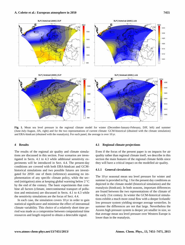
Fig. 1. Mean sea level pressure in the regional climate model for winter (December-January-February, DJF, left) and summer(June-July-August, JJA, right) and for the two representations of current climate: GCM-historical (obtained with the climate simulation)and ERA-hindcast (obtained with the reanalysis). For each panel, the average is over 10 yr.

4 Results

The results of the regional air quality and climate simula-tions are discussed in this section. Four scenarios are inves-tigated in Sects. 4.1 to 4.3 while additional sensitivity ex-periments will be introduced in Sect. 4.4. The present-dayconditions are covered with both ERA-hindcast and GCM-historical simulations and two possible futures are investi-gated for 2050: one of them (reference) assuming no im-plementation of any specific climate policy, while the sec-ond (mitigation) aims at keeping global warming below 2◦Cby the end of the century. The basic experiments that com-bine all factors (climate, intercontinental transport of pollu-tion and emissions) are discussed in Sects. 4.1 to 4.3 whilethe sensitivity simulations are the focus of Sect. 4.4.

In each case, the simulation covers 10 yr in order to gainstatistical significance and minimise the effect of interannualclimate variability. This choice of a relatively short time pe-riod was made as a compromise between computational timeresources and length required to obtain a detectable signal.

4.1 Regional climate projections

Even if the focus of the present paper is on impacts for airquality rather than regional climate itself, we describe in thissection the main features of the regional climate fields sincethey will have a critical impact on the modelled air quality.

4.1.1 General circulation

The 10 yr seasonal mean sea level pressure for winter andsummer is provided in Fig. 1 for the present day conditions asdepicted in the climate model (historical simulation) and thereanalysis (hindcast). In both seasons, important differencesare found between the two representations of the climate ofthe early 21st century. In winter the GCM-historical simula-tions exhibit a much more zonal flow with a deeper Icelandiclow pressure system yielding stronger average westerlies. Insummer the differences are not that large. Nevertheless theAzores high pressure system is deeper yet smaller in size, sothat average mean sea level pressure over Western Europe islower than in the reanalysis.

www.atmos-chem-phys.net/13/7451/2013/ Atmos. Chem. Phys., 13, 7451–7471, 2013

7456 A. Colette et al.: European atmosphere in 2050

35

1

Figure 2 : Left column: summer time (JJA) high 2-m daily mean temperatures (95th quantile, K) 2

and right column: annual mean liquid precipitation (mm/day). On the first row we display the 3

absolute results of the GCM-historical climate simulation and on the following row the 4

differences compared to the later for the ERA-hindcast, the 2050 reference and the 2050 5

mitigation projections. 6

Fig. 2. Left column panels: summertime (JJA) high 2 m daily mean temperatures (95th quantile, K) and right column panels: annual meanliquid precipitation (mm day−1). On the first row we display the absolute results of the GCM-historical climate simulation and on thefollowing row the differences compared to the later for the ERA-hindcast, the 2050 reference and the 2050 mitigation projections.

Atmos. Chem. Phys., 13, 7451–7471, 2013 www.atmos-chem-phys.net/13/7451/2013/

A. Colette et al.: European atmosphere in 2050 7457

4.1.2 Temperature and precipitation

The higher end of the temperature distribution also differsstrongly when changing the large-scale forcing. As shownin Fig. 2, the GCM-historical climate model is much colderthan the reanalysed ERA-hindcast. This statement is true forboth annual mean temperature (−0.9 K in winter and−1.5 Kin summer) and the 95th percentile of summer daily meantemperature (left panels in Fig. 2) with an average bias overWestern Europe (5◦ W–15◦ E, 40–55◦ N; see area in Fig. 8) of−1.6 K. This average bias is partly compensated by an oppo-site bias over sea surfaces. Over continental areas the temper-ature bias can reach values as high as 5 K. It is noteworthy toemphasise that the 95th percentile of temperature in the 2050projections is respectively 1.9 K (for the RCP8.5) and 0.5 K(RCP2.6) warmer than the GCM-historical climate, show-ing that the absolute differences between current and futureclimate are actually smaller than temperature biases in thepresent climate.

Differences in daily precipitation are also shown (rightpanels in Fig. 2). Precipitation is a key variable for air qual-ity because it drives wet scavenging which is an importantsink for some trace species. The second row in Fig. 2 showsthat the GCM-historical climate simulation is too wet com-pared to the reanalysis throughout Europe. For precipitation,the difference between the current and projected climate isalso clearly lower than the differences of the two realisationsof current climate.

4.1.3 Summary

Sections 4.1.1 to 4.1.3 have shown important differences be-tween the reanalysed and climate simulations that will beused to drive the air quality modelling performed in the re-mainder of the study. We anticipate some of these features tohave a detrimental impact on the simulation of air pollutantevents.

It is not the purpose of this study to assess where suchdifferences come from. Briefly, we can point towards (1)the global climate model, (2) the dynamical regional cli-mate downscaling, or (3) the choice of the time period. TheIPSL-CM5-MR model is known to exhibit a cold bias ofsea surface temperature over the North Atlantic as a resultof a strong underestimation of the Atlantic meridional over-turning circulation (Hourdin et al., 2012). The dynamicaldownscaling has been demonstrated to contribute to an ad-ditional cooling (Colette et al., 2012c; Menut et al., 2012).These discrepancies could also be an artefact of the rela-tively short time period (10 yr) that could be influenced byan unfavourable climate mode (of the North Atlantic Oscil-lation for instance). The importance of using long times se-ries has been repeatedly emphasized in climate studies andthis factor should be taken into account in future air qualityand climate assessments when the computing resources aresufficient (Langner et al., 2012a).

Before concluding this section devoted to the climate pro-jection it is important to keep in mind that it is not becausethe climate model exhibits a bias that its projected changesare not valid. An over-fitted climate would perform ideallyfor the past, yet being very poor for future projections. Thatis why, in the vast majority of the climate science litera-ture, model variability is investigated rather than absolutechanges. For that respect, climate sensitivity is a more rel-evant metric than biases over a given period, and the climatesensitivity of the IPSL-CM5-LR model was found to fit in themiddle of the ensemble of CMIP5 models (Vial et al., 2013).However, when it comes to climate impact modelling abso-lute differences and biases do matter, hence raising new chal-lenges. Besides, in the field of climate research, confidenceis achieved by making use of model ensembles, which raisesa significant computational challenge for air quality projec-tions (that would ideally be based on ensembles of each ofthe four types of models introduced in Sect. 3, hence mul-tiplying the size of the ensemble). We will discuss in moredetail throughout the remainder of the paper how such differ-ences bear upon our confidence in air quality projections.

4.2 Evaluation of air quality simulations

Before discussing the modelled changes in air qualityat the horizon 2050, we compare the air quality resultsfor the present day to observations. We use ozone (dailymax) and PM10 (daily mean) recorded at air qualitymonitoring stations (1108 for ozone and 688 for PM10)available for the 1998–2007 period in the AIRBASEpublic air quality database maintained by the EuropeanEnvironmental Agency (http://air-climate.eionet.europa.eu/databases/AIRBASE/). Synchronous scores (correlation asR2 and root mean square error, RMSE) are computed for theair quality simulations driven with the ERA-hindcast meteo-rological fields, whereas only average biases are provided forGCM-historical that relies on a different meteorology.

The results in Table 2 are in-line with previous implemen-tation of CHIMERE (Solazzo et al., 2012a, b; van Loon etal., 2007) in particular when using this set-up (Colette et al.,2011, 2012a). A positive bias is found for ozone which isexpected at such a coarse resolution where primary emis-sions are smeared out. This bias is partly compensated bya good correlation to achieve a satisfactory RMSE. The cli-mate (GCM-historical) forcing tends to produce much lessozone, hence the small negative bias while a positive ozonebias would be expected at such a coarse resolution. For par-ticulate matter a significant negative bias is found. This rangeof bias is a common feature in many operational air qualitymodels (Solazzo et al., 2012a), in the present case the bias iseven increased because we use only black and organic carbonemissions and ignore other anthropogenic primary particu-late matter sources (even though we do account for naturaland secondary PM, see Sect. 4.3.2).

www.atmos-chem-phys.net/13/7451/2013/ Atmos. Chem. Phys., 13, 7451–7471, 2013

7458 A. Colette et al.: European atmosphere in 2050

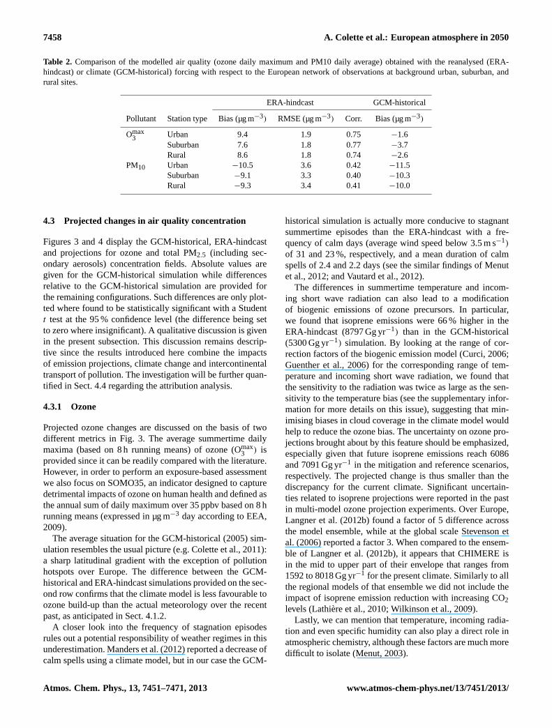
Table 2. Comparison of the modelled air quality (ozone daily maximum and PM10 daily average) obtained with the reanalysed (ERA-hindcast) or climate (GCM-historical) forcing with respect to the European network of observations at background urban, suburban, andrural sites.

ERA-hindcast GCM-historical

Pollutant Station type Bias (µg m−3) RMSE (µg m−3) Corr. Bias (µg m−3)

Omax3 Urban 9.4 1.9 0.75 −1.6

Suburban 7.6 1.8 0.77 −3.7Rural 8.6 1.8 0.74 −2.6

PM10 Urban −10.5 3.6 0.42 −11.5Suburban −9.1 3.3 0.40 −10.3Rural −9.3 3.4 0.41 −10.0

4.3 Projected changes in air quality concentration

Figures 3 and 4 display the GCM-historical, ERA-hindcastand projections for ozone and total PM2.5 (including sec-ondary aerosols) concentration fields. Absolute values aregiven for the GCM-historical simulation while differencesrelative to the GCM-historical simulation are provided forthe remaining configurations. Such differences are only plot-ted where found to be statistically significant with a Studentt test at the 95 % confidence level (the difference being setto zero where insignificant). A qualitative discussion is givenin the present subsection. This discussion remains descrip-tive since the results introduced here combine the impactsof emission projections, climate change and intercontinentaltransport of pollution. The investigation will be further quan-tified in Sect. 4.4 regarding the attribution analysis.

4.3.1 Ozone

Projected ozone changes are discussed on the basis of twodifferent metrics in Fig. 3. The average summertime dailymaxima (based on 8 h running means) of ozone (Omax

3 ) isprovided since it can be readily compared with the literature.However, in order to perform an exposure-based assessmentwe also focus on SOMO35, an indicator designed to capturedetrimental impacts of ozone on human health and defined asthe annual sum of daily maximum over 35 ppbv based on 8 hrunning means (expressed in µg m−3 day according to EEA,2009).

The average situation for the GCM-historical (2005) sim-ulation resembles the usual picture (e.g. Colette et al., 2011):a sharp latitudinal gradient with the exception of pollutionhotspots over Europe. The difference between the GCM-historical and ERA-hindcast simulations provided on the sec-ond row confirms that the climate model is less favourable toozone build-up than the actual meteorology over the recentpast, as anticipated in Sect. 4.1.2.

A closer look into the frequency of stagnation episodesrules out a potential responsibility of weather regimes in thisunderestimation. Manders et al. (2012) reported a decrease ofcalm spells using a climate model, but in our case the GCM-

historical simulation is actually more conducive to stagnantsummertime episodes than the ERA-hindcast with a fre-quency of calm days (average wind speed below 3.5 m s−1)

of 31 and 23 %, respectively, and a mean duration of calmspells of 2.4 and 2.2 days (see the similar findings of Menutet al., 2012; and Vautard et al., 2012).

The differences in summertime temperature and incom-ing short wave radiation can also lead to a modificationof biogenic emissions of ozone precursors. In particular,we found that isoprene emissions were 66 % higher in theERA-hindcast (8797 Gg yr−1) than in the GCM-historical(5300 Gg yr−1) simulation. By looking at the range of cor-rection factors of the biogenic emission model (Curci, 2006;Guenther et al., 2006) for the corresponding range of tem-perature and incoming short wave radiation, we found thatthe sensitivity to the radiation was twice as large as the sen-sitivity to the temperature bias (see the supplementary infor-mation for more details on this issue), suggesting that min-imising biases in cloud coverage in the climate model wouldhelp to reduce the ozone bias. The uncertainty on ozone pro-jections brought about by this feature should be emphasized,especially given that future isoprene emissions reach 6086and 7091 Gg yr−1 in the mitigation and reference scenarios,respectively. The projected change is thus smaller than thediscrepancy for the current climate. Significant uncertain-ties related to isoprene projections were reported in the pastin multi-model ozone projection experiments. Over Europe,Langner et al. (2012b) found a factor of 5 difference acrossthe model ensemble, while at the global scale Stevenson etal. (2006) reported a factor 3. When compared to the ensem-ble of Langner et al. (2012b), it appears that CHIMERE isin the mid to upper part of their envelope that ranges from1592 to 8018 Gg yr−1 for the present climate. Similarly to allthe regional models of that ensemble we did not include theimpact of isoprene emission reduction with increasing CO2levels (Lathiere et al., 2010; Wilkinson et al., 2009).

Lastly, we can mention that temperature, incoming radia-tion and even specific humidity can also play a direct role inatmospheric chemistry, although these factors are much moredifficult to isolate (Menut, 2003).

Atmos. Chem. Phys., 13, 7451–7471, 2013 www.atmos-chem-phys.net/13/7451/2013/

A. Colette et al.: European atmosphere in 2050 7459

36

Figure 3: Top row (from left to right): average fields of ozone as summertime average of the

daily maxima (O3max, µg m-3), and SOMO35 (µg m-3 day) in the control (2005) simulation

(averaged over 10 years corresponding to the current climate). Following rows: difference

Fig. 3.Top row panels(from left to right): average fields of ozone as summertime average of the daily maxima (Omax3 , µg m−3), and SOMO35

(µg m−3 day) in the control (2005) simulation (averaged over 10 yr corresponding to the current climate). Following panel rows: differencebetween the simulations for the reanalysed ERA-hindcast and then for the reference and mitigation 2050 projections taken with respect tothe GCM-historical climate simulation (2005). The differences are only displayed where significant given the interannual variability of 10 yr.

Both projections for 2050 indicate a decrease of dailymaximum ozone compared to the GCM-historical climatesimulation, but the magnitude of this decrease is moderatefor the reference scenario. The situation is however more

complex under the reference scenario for the human healthexposure to ozone, since the index SOMO35 actually in-creases over a significant part of Europe. The mitigation sce-nario achieves a much higher degree of emission reduction.

www.atmos-chem-phys.net/13/7451/2013/ Atmos. Chem. Phys., 13, 7451–7471, 2013

7460 A. Colette et al.: European atmosphere in 2050

As a result, SOMO35 decreases sharply, especially in theMediterranean area where the levels were highest. On amore quantitative basis, in order to emphasise the projectedchanges in high-exposure areas, we apply a weighting func-tion to the SOMO35 fields depending on the population den-sity (obtained from Riahi et al., 2012; and United Nations,2009, but using the population for 2005 for both the cur-rent and prospective scenarios). We find that the population-weighted SOMO35 increases by 7.4 % (standard deviation±5.4 %) in the reference scenario whereas it decreases by80.4 % (±2.1 %) in the mitigation case.

4.3.2 Particulate matter

In addition to the primary particulate matter prescribed inthe anthropogenic emissions (elemental carbon – EC – andorganic carbon – OC) and derived in the natural emissions(dust and sea salt), CHIMERE accounts for the formationof secondary aerosols that undergo a range of microphys-ical transformations including nucleation, coagulation, andabsorption. For inorganic species such as nitrate (NO3), sul-phate (SO4) and ammonium (NH4) the thermodynamic equi-librium is diagnosed using the ISORROPIA model (Neneset al., 1998). For semi-volatile organic species, a partitioncoefficient is used (Pankow, 1994). Chemical formation ofsecondary organic aerosols (SOA) is represented with a sin-gle step oxidation of the relevant precursors and gas-particlepartitioning of the condensable oxidation products (Bessag-net et al., 2008a). Most SOA are issued from the oxidation ofmonoterpenes computed with the MEGAN model (Guentheret al., 2006). The processes related to aerosol dynamics aredescribed in Bessagnet et al. (2004).

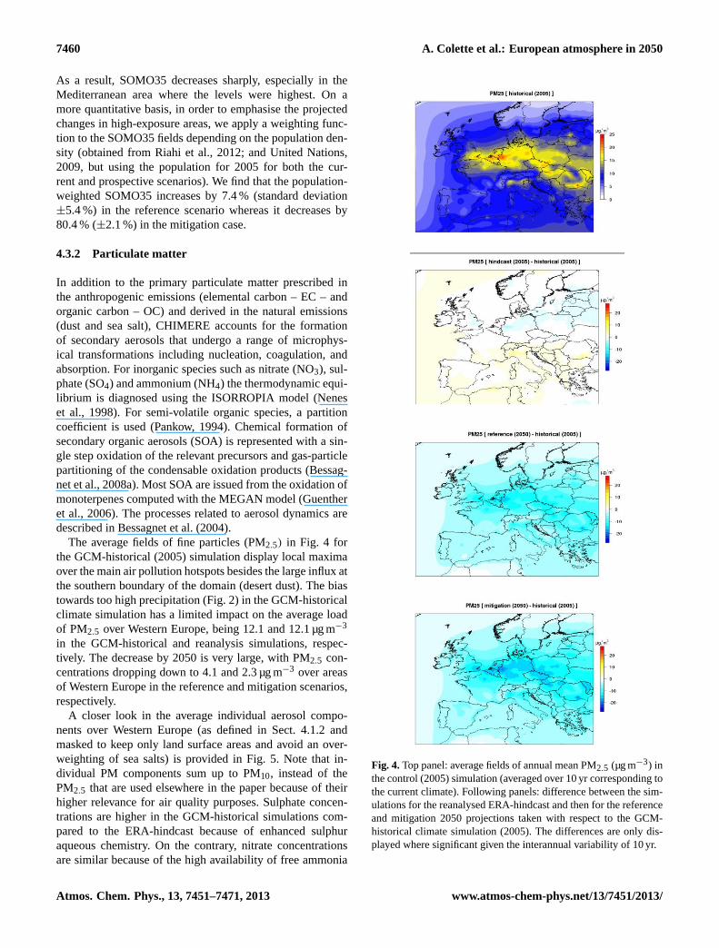
The average fields of fine particles (PM2.5) in Fig. 4 forthe GCM-historical (2005) simulation display local maximaover the main air pollution hotspots besides the large influx atthe southern boundary of the domain (desert dust). The biastowards too high precipitation (Fig. 2) in the GCM-historicalclimate simulation has a limited impact on the average loadof PM2.5 over Western Europe, being 12.1 and 12.1 µg m−3

in the GCM-historical and reanalysis simulations, respec-tively. The decrease by 2050 is very large, with PM2.5 con-centrations dropping down to 4.1 and 2.3 µg m−3 over areasof Western Europe in the reference and mitigation scenarios,respectively.

A closer look in the average individual aerosol compo-nents over Western Europe (as defined in Sect. 4.1.2 andmasked to keep only land surface areas and avoid an over-weighting of sea salts) is provided in Fig. 5. Note that in-dividual PM components sum up to PM10, instead of thePM2.5 that are used elsewhere in the paper because of theirhigher relevance for air quality purposes. Sulphate concen-trations are higher in the GCM-historical simulations com-pared to the ERA-hindcast because of enhanced sulphuraqueous chemistry. On the contrary, nitrate concentrationsare similar because of the high availability of free ammonia

38

Figure 4 : Top row (from left to right): average fields of annual mean PM2.5 (µg m-3) in the

control (2005) simulation (averaged over 10 years corresponding to the current climate).

Following rows: difference between the simulations for the reanalysed ERA-hindcast and then

Fig. 4.Top panel: average fields of annual mean PM2.5 (µg m−3) inthe control (2005) simulation (averaged over 10 yr corresponding tothe current climate). Following panels: difference between the sim-ulations for the reanalysed ERA-hindcast and then for the referenceand mitigation 2050 projections taken with respect to the GCM-historical climate simulation (2005). The differences are only dis-played where significant given the interannual variability of 10 yr.

Atmos. Chem. Phys., 13, 7451–7471, 2013 www.atmos-chem-phys.net/13/7451/2013/

A. Colette et al.: European atmosphere in 2050 7461

39

for the reference and mitigation 2050 projections taken with respect to the GCM-historical

climate simulation (2005). The differences are only displayed where significant given the

interannual variability of ten years.

Figure 5 : Average aerosol composition over land surfaces of Western Europe for the two

simulations corresponding to the present-day conditions (GCM-historical and ERA-hindcast) as

well as the two scenarios for 2050 (Reference and Mitigation). Absolute concentrations are

given on the left panel and relative contributions to total PM10 (expressed in percentages) are

given on the right panel.

Fig. 5. Average aerosol composition over land surfaces of WesternEurope for the two simulations corresponding to the present-dayconditions (GCM-historical and ERA-hindcast) as well as the twoscenarios for 2050 (reference and mitigation). Absolute concentra-tions are given on the left panel and relative contributions to totalPM10 (expressed in percentages) are given on the right panel.

(defined as the total ammonia minus sulphate, in moles) inthe atmosphere.

All the secondary aerosols decrease in the future as a re-sult of decreasing anthropogenic emission of precursors. Themost prominent feature in the projection of aerosol compo-sition is the increase of the relative importance of naturalaerosols such as dust and sea salts in the future (right panelin Fig. 5), so that in the most stringent scenario the fractionof crustal material becomes dominant in PM10. Secondaryorganic aerosols are the only species that maintain their rel-ative importance due to the contribution of biogenic precur-sors in their formation process. As far as secondary inorganicaerosols are concerned it is worth mentioning that the smallincrease of NH3 emissions in the GEA projections – Table 1and Colette et al. (2012b) – is not reflected in the projectedformation of particulate NH+4 . Whereas NH3 emissions in-crease by 22 and 21 % for the reference and mitigation sce-narios, respectively. Between 2005 and 2050, we find thatNH+

4 decreases from 4.0 µg m−3 in the GCM-historical 2005simulation to 1.4 and 0.5 µg m−3 in the reference and miti-gation projections, respectively. This feature emphasises theprobable limiting role of NOx emissions through the avail-ability of HNO3 in rural areas (Hamaoui-Laguel et al., 2012)that do exhibit a strong decrease in the future. The reasonwhy such behaviour is not reported in coarse global chem-istry transport model projections deserves further investiga-tion (Fiore et al., 2012; Shindell et al., 2013). While in thehistorical simulations nitrate represents about 33 % of non-natural particles, this fraction reaches 39–42 % in 2050.

In terms of exposure, we find that population-weightedPM2.5 decreases by 61.8 (±3.1) and 78.0 % (±1.8) in thereference and mitigation scenarios, respectively. It appearsthat air quality legislation (which is identical in both sce-narios) somewhat dominates the relative change in exposure

to PM2.5, the impact of the climate policy (which differs inboth scenarios) is not as large as observed for the exposureto ozone.

4.4 Disentangling the driving factors

The projected exposure to air pollution discussed in Sect. 4.3takes into account the whole range of processes playing a rolein the future evolution of air quality: global and regional cli-mate, chemical background changes as well as air pollutionmitigation measures. This modelling system also offers theopportunity to isolate the contribution of each driving fac-tor to the overall projected change in the basic simulationsdiscussed in Sect. 4.3.

4.4.1 Methodology

We quantify the respective role of each process from sensi-tivity experiments consisting in replicating the decadal sim-ulations with all things kept equal except one of the drivingfactors.

The list of simulation experiments is synthesised in Ta-ble 3 which includes both the reference and mitigation pro-jections. Only present and future time periods are given inthe table, and the future time period refers to either the ref-erence (CLE1 for AP emissions, RCP8.5 for climate andboundary conditions) or the mitigation (CLE2 for AP emis-sions, RCP2.6 for climate and boundary conditions). Eachrow of the table refers to the isolation of one driving process,which is achieved by comparing the experiment described inthe middle columns to the experiment described in the rightcolumns.

The overall impact of climate, boundary conditions andAP emissions is obtained from the basic simulations (firstrow from the bottom). The second row from the bottom pro-vides the specification of the simulation used to isolate theimpact of switching from reanalyses to a climate model forthe present conditions. In order to investigate the regionaleffects of climate change, the first step consists in using con-stant present-day AP emission and boundary conditions andthen changing the climate forcing (third row from the bot-tom). However, in order to explore the climate response un-der gradually changing AP emissions – yet avoiding per-forming transient simulation – the sensitivity to regional cli-mate change is also tested with future AP emissions (fourthrow from the bottom). Symmetrically, the impact of emis-sions under constant climate and boundary conditions is ex-plored for the present climate and the future climate. Last,the impact of boundary conditions is derived from the exper-iment on the 7th row from the bottom. We decided to ignorethe impact of gradually changing climate and emissions onthe role of the boundary conditions, in order to avoid increas-ing the dimension of the sensitivity matrix to be explored.

Some of the simulations are used several times in the pro-cess, so that only the unique sensitivity experiments are bold.

www.atmos-chem-phys.net/13/7451/2013/ Atmos. Chem. Phys., 13, 7451–7471, 2013

7462 A. Colette et al.: European atmosphere in 2050

Five unique sensitivity decadal simulations are required foreach of the two (reference and mitigation) scenarios, plustwo baselines for the present day (ERA-hindcast and GCM-historical) that are common to both scenarios. In total, wehave thus twelve decadal regional air quality simulations.

The results are provided in Figs. 6 and 7 as box plots re-ferring to the key provided in Table 3.

Each sensitivity simulation is decadal. Instead of givingthe difference of the temporal averages (such as on the mapsin the previous figures), we first aggregate spatially by tak-ing the mean over Western Europe (5◦ W–15◦ E, 40–55◦ N)and then we compute the distribution of differences betweenthe two sets of decadal simulations, which are 55 indepen-dent combinations of individual years. These distributions of55 differences are presented here as box and whisker plotswhere the boxes provide the three inner quartiles and thewhiskers provide the extremes of the distribution. A crossis given where the distribution of difference is statisticallysignificantly different from zero (Student’st test with a 95 %confidence interval).

Multi-annual sensitivity experiments are common prac-tice in climate studies, but annual simulations are often usedin atmospheric chemistry studies to investigate the impactof emission changes or boundary conditions. However, thespread of the distributions obtained here demonstrate theneed to use multi-annual sensitivity simulations in order toprovide a quantitative perspective of the uncertainty whereasthe qualitative conclusions would be unchanged.

The differences between the sensitivity experiments per-formed under present-day or future conditions (the twoshades of orange and blue) also emphasise the need to ex-plore the impact of regional climate change and AP emis-sions under gradually changing conditions. Whereas the rel-evance of transient approaches are often pointed out in base-case projections (Langner et al., 2012a), it is not commonpractice in sensitivity experiments addressing the disentan-gling of various contributions (Hedegaard et al., 2013; Man-ders et al., 2012), while Figs. 6 and 7 show that the evolutionof the response to climate or emission changes differs underpresent day and future conditions.

4.4.2 Results

Ozone

Ozone is presented here (Fig. 6), as in Sect. 4.3, as the av-erage summertime of daily maximum based on 8 h runningmeans as well as SOMO35 and we find again that the over-all projection (including all factors: white boxes) consists ina decrease by 2050 for both scenarios for Omax

3 and for themitigation scenario for SOMO35, while a small increase isfound under the reference scenario for SOMO35. In all casesthe changes are statistically significant.

We find that the role of AP emissions change (boxes inblue shadings) dominates over the impact of regional climate

change (boxes in orange shadings). For SOMO35, the rel-ative change attributed to climate ranges from 3 (±8 %) to5 % (±11 %), while the response when changing emissionsranges from−24 (±10 %) to−43 % (±7 %). Recent studieson ozone projections relying on air pollutant emissions pre-scribed by the RCPs also reported that anthropogenic emis-sion changes dominate over the effect of climate (Fiore etal., 2012; Hedegaard et al., 2013; Katragkou et al., 2011;Langner et al., 2012a, b; Lei et al., 2012; Manders et al.,2012). The fact that we use air pollutant emission projectionsbased on explicit mitigation policies adds robustness to thisfinding.

Regional climate is found to constitute a significantpenalty on ozone under present-day emissions (dark orangebox) according to all metrics and scenarios. However, theresponse is not that large: below about 1 µg m−3 for Omax

3 .This moderate impact is not surprising compared to the fig-ures reported elsewhere where differences rarely exceed afew µg m−3 (Andersson and Engardt, 2010; Katragkou et al.,2011; Langner et al., 2012a, b), only Manders et al. (2012)found increases that could reach 5–10 µg m−3. A more in-novative finding lies in the assessment of the climate penaltyunder future AP emission (light orange box). We find that thepenalty will decrease in magnitude and even become a netbenefit for Omax

3 under the mitigation scenario. The fact thatprojected climate change can contribute to decrease ozonelevels on average over Western Europe was never reportedbefore and highlights the need to account for the AQ policieswhen addressing the climate penalty. Whereas there are ex-amples in the literature of assessments including combinedclimate and emission changes, sensitivity attribution studiesare systematically performed under present-day conditions.We show here that the future context must be accounted for,even in the sensitivity analysis.

Ozone projections over Western Europe are actually moresensitive to background concentrations changes than to thepenalty/benefit brought about by regional climate change.The tropospheric background ozone change constitutes apenalty under the reference scenario and a benefit under themitigation case. These opposite trends stem from the jointevolution of global emissions and global climate and werealso reported in the global chemistry–climate projections forthese scenarios (Szopa et al., 2012; Young et al., 2013). Itis worth emphasising that in the global CTM, chemistry andclimate are addressed jointly, it is therefore not possible toisolate to what extent these opposite trends are a result of APemission changes in distant areas or a result of global climateon chemistry. In the mitigation scenario the decreasing back-ground ozone burden contributes to increasing the benefit al-ready obtained thanks to the reduction of AP emissions. Butin the reference scenario, the compensation between a lowermagnitude of AP emission changes and a penalty broughtabout by the increasing ozone background yields the penaltyseen for SOMO35 in the net response.

Atmos. Chem. Phys., 13, 7451–7471, 2013 www.atmos-chem-phys.net/13/7451/2013/

A. Colette et al.: European atmosphere in 2050 7463

40

Figure 6: Contribution of the background air pollution (Bckd, violet), regional emissions (Emiss.,

blue shadings), and climate change (GCM, orange shadings) to the total projected changes

(white) in O3 concentration as summer average of the daily max (O3max), and SOMO35 averaged

over Western Europe in 2050 according to the reference (left) and mitigation (right) scenarios.

In each case, we display net differences compared to a control selected to isolate one of the

factor. The sensitivity to the meteorological driver (either GCM-historical climate or ERA-

hindcast) is also given (ERA, brown). The sensitivity to emission and climate is investigated for

both present and future conditions, hence the duplicate blue and orange boxes. A cross is

marked when the distribution is significantly different from zero. The bottom axis provides the

absolute difference and the relative difference with regards to the GCM-historical simulation is

given as percentages on the top axis.

Fig. 6. Contribution of the background air pollution (Bckd, violet), regional emissions (Emiss., blue shadings), and climate change (GCM,orange shadings) to the total projected changes (white) in O3 concentration as summer average of the daily max (Omax

3 ), and SOMO35 aver-aged over Western Europe in 2050 according to the reference (left) and mitigation (right) scenarios. In each case, we display net differencescompared to a control selected to isolate one of the factors. The sensitivity to the meteorological driver (either GCM-historical climate orERA-hindcast) is also given (ERA, brown). The sensitivity to emission and climate is investigated for both present and future conditions,hence the duplicate blue and orange boxes. A cross is marked when the distribution is significantly different from zero. The bottom axisprovides the absolute difference and the relative difference with regards to the GCM-historical simulation is given as percentages on the topaxis.

41

Figure 7: Contribution of the background air pollution (Bckd, violet), regional emissions (Emiss.,

blue shadings), and climate change (GCM, orange shadings) to the total projected changes

(white) in annual mean PM2.5 over Western Europe in 2050 according to the reference (left)

and mitigation (right) scenarios. In each case, we display net differences compared to a control

selected to isolate one of the factor. The sensitivity to the meteorological driver (either GCM-

historical climate or ERA-hindcast) is also given (ERA, brown). The sensitivity to emission and

climate is investigated for both present and future conditions, hence the duplicate blue and

orange boxes. A cross is marked when the distribution is significantly different from zero. The

bottom axis provides the absolute difference and the relative difference with regards to the

GCM-historical simulation is given as percentages on the top axis.

Fig. 7. Contribution of the background air pollution (Bckd, violet), regional emissions (Emiss., blue shadings), and climate change (GCM,orange shadings) to the total projected changes (white) in annual mean PM2.5 over Western Europe in 2050 according to the reference(left) and mitigation (right) scenarios. In each case, we display net differences compared to a control selected to isolate one of the factors.The sensitivity to the meteorological driver (either GCM-historical climate or ERA-hindcast) is also given (ERA, brown). The sensitivity toemission and climate is investigated for both present and future conditions, hence the duplicate blue and orange boxes. A cross is markedwhen the distribution is significantly different from zero. The bottom axis provides the absolute difference and the relative difference withregards to the GCM-historical simulation is given as percentages on the top axis.

www.atmos-chem-phys.net/13/7451/2013/ Atmos. Chem. Phys., 13, 7451–7471, 2013

7464 A. Colette et al.: European atmosphere in 2050

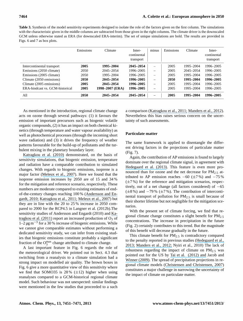
Table 3.Synthesis of the model sensitivity experiments designed to isolate the role of the factors given on the first column. The simulationswith the characteristic given in the middle columns are subtracted from those given in the right columns. The climate driver is the downscaledGCM unless otherwise stated as ERA (for downscaled ERA-interim). The set of unique simulations are bold. The results are provided inFigs. 6 and 7 as box plots.

Emissions Climate Inter- minus Emissions Climate Inter-continental continentaltransport transport

Intercontinental transport 2005 1995–2004 2045–2054 – 2005 1995–2004 1996–2005Emissions (2050 climate) 2050 2045–2054 1996–2005 – 2005 2045–2054 1996–2005Emissions (2005 climate) 2050 1995–2004 1996–2005 – 2005 1995–2004 1996–2005Climate (2050 emissions) 2050 2045–2054 1996–2005 – 2050 1995–2004 1996–2005Climate (2005 emissions) 2005 2045–2054 1996–2005 – 2005 1995–2004 1996–2005ERA-hindcast vs. GCM-historical 2005 1998–2007 (ERA) 1996–2005 – 2005 1995–2004 1996–2005

All 2050 2045–2054 2045–2054 – 2005 1995–2004 1996–2005

As mentioned in the introduction, regional climate changeacts on ozone through several pathways: (1) it favours theemission of important precursors such as biogenic volatileorganic compounds, (2) it has an impact on both chemical ki-netics (through temperature and water vapour availability) aswell as photochemical processes (through the incoming shortwave radiation) and (3) it drives the frequency of weatherpatterns favourable for the build-up of pollutants and the tur-bulent mixing in the planetary boundary layer.

Katragkou et al. (2010) demonstrated, on the basis ofsensitivity simulations, that biogenic emission, temperatureand radiation have a comparable contribution to simulatedchanges. With regards to biogenic emissions, isoprene is amajor factor (Meleux et al., 2007). Here we found that theisoprene emission increases by 2050 are of 15 and 34 %for the mitigation and reference scenario, respectively. Thesenumbers are moderate compared to existing estimates of end-of-the-century changes reaching 100 % (Andersson and En-gardt, 2010; Katragkou et al., 2011; Meleux et al., 2007) butthey are in line with the 20 to 25 % increase in 2050 com-pared to 2000 for the RCP4.5 in Langner et al. (2012b).Thesensitivity studies of Andersson and Engardt (2010) and Ka-tragkou et al. (2011) report an increased production of O3 of1–2 µg m−3 for a 30 % increase of biogenic emissions. Whilewe cannot give comparable estimates without performing adedicated sensitivity study, we can infer from existing stud-ies that biogenic emissions constitute probably a significantfraction of the Omax

3 change attributed to climate change.A last important feature in Fig. 6 regards the role of

the meteorological driver. We pointed out in Sect. 4.3 thatswitching from a reanalysis to a climate simulation had astrong impact on modelled air quality. The brown boxes inFig. 6 give a more quantitative view of this sensitivity wherewe find that SOMO35 is 28 % (±12) higher when usingreanalyses compared to a GCM-historical regional climatemodel. Such behaviour was not unexpected: similar findingswere mentioned in the few studies that proceeded to a such

a comparison (Katragkou et al., 2011; Manders et al., 2012).Nevertheless this bias raises serious concern on the uncer-tainty of such assessments.

Particulate matter

The same framework is applied to disentangle the differ-ent driving factors in the projections of particulate matter(Fig. 7).

Again, the contribution of AP emissions is found to largelydominate over the regional climate signal, in agreement withHedegaard et al. (2013). This feature is even more pro-nounced than for ozone and the net decrease for PM2.5 at-tributed to AP emission reaches−60 (±7 %) and−75 %(±7 %) for the reference and mitigation scenarios, respec-tively, out of a net change (all factors considered) of−65(±8 %) and−79 % (±7 %). The contribution of interconti-nental transport of pollution for PM2.5 is small because oftheir shorter lifetime but not negligible for the mitigation sce-narios.

With the present set of climate forcing, we find that re-gional climate change constitutes a slight benefit for PM2.5concentrations. The increase in precipitation in the future(Fig. 2) certainly contributes to this trend. But the magnitudeof this benefit will decrease gradually in the future.

This climate benefit for PM2.5 is contradictory comparedto the penalty reported in previous studies (Hedegaard et al.,2013; Manders et al., 2012; Nyiri et al., 2010) The lack ofrobustness regarding the impact of climate on PM2.5 waspointed out for the US by Tai et al. (2012) and Jacob andWinner (2009). The spread of precipitation projections in re-gional climate models (Christensen and Christensen, 2007)constitutes a major challenge in narrowing the uncertainty ofthe impact of climate on particulate matter.

Atmos. Chem. Phys., 13, 7451–7471, 2013 www.atmos-chem-phys.net/13/7451/2013/

A. Colette et al.: European atmosphere in 2050 7465

42

Figure 8: Map of the contribution of the regional climate to the projected change in air quality

(from top to bottom: SOMO35, and PM2.5) for the reference (left) and mitigation (right)

scenarios. A positive sign (red) indicates a climate penalty (increase air pollutant

concentrations), whereas a negative sign (blue) shows that future climate tends to reduce

detrimental air pollution levels.

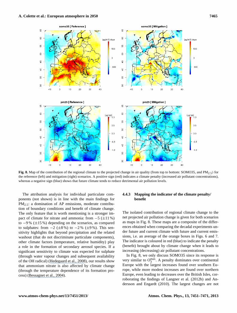
Fig. 8. Map of the contribution of the regional climate to the projected change in air quality (from top to bottom: SOMO35, and PM2.5) forthe reference (left) and mitigation (right) scenarios. A positive sign (red) indicates a climate penalty (increased air pollutant concentrations),whereas a negative sign (blue) shows that future climate tends to reduce detrimental air pollution levels.

The attribution analysis for individual particulate com-ponents (not shown) is in line with the main findings forPM2.5: a domination of AP emissions, moderate contribu-tion of boundary conditions and benefit of climate change.The only feature that is worth mentioning is a stronger im-pact of climate for nitrate and ammonia: from−5 (±11 %)to −9 % (±15 %) depending on the scenarios, as comparedto sulphates: from−2 (±8 %) to −2 % (±9 %). This sen-sitivity highlights that beyond precipitation and the relatedwashout (that do not discriminate particulate components),other climate factors (temperature, relative humidity) playa role in the formation of secondary aerosol species. If asignificant sensitivity to climate was expected for sulphate(through water vapour changes and subsequent availabilityof the OH radical) (Hedegaard et al., 2008), our results showthat ammonium nitrate is also affected by climate change(through the temperature dependence of its formation pro-cess) (Bessagnet et al., 2004).

4.4.3 Mapping the indicator of the climate penalty/benefit

The isolated contribution of regional climate change to thenet projected air pollution change is given for both scenariosas maps in Fig. 8. These maps are a composite of the differ-ences obtained when comparing the decadal experiments un-der future and current climate with future and current emis-sions, i.e. an average of the orange boxes in Figs. 6 and 7.The indicator is coloured in red (blue) to indicate the penalty(benefit) brought about by climate change when it leads toincreasing (decreasing) air pollutant concentrations.

In Fig. 8, we only discuss SOMO35 since its response isvery similar to Omax

3 . A penalty dominates over continentalEurope with the largest increases found over southern Eu-rope, while more modest increases are found over northernEurope, even leading to decreases over the British Isles, cor-roborating the findings of Langner et al. (2012b) and An-dersson and Engardt (2010). The largest changes are not

www.atmos-chem-phys.net/13/7451/2013/ Atmos. Chem. Phys., 13, 7451–7471, 2013

7466 A. Colette et al.: European atmosphere in 2050

systematically located over areas exhibiting high ozone lev-els such as the Mediterranean, emphasising the role of bio-genic precursors (Meleux et al., 2007).

For PM2.5, regional climate change constitutes mostly abenefit by decreasing the concentrations. Over Morocco apenalty is found, which can be related to the decrease of pre-cipitation in this area (Fig. 2). The penalty over the NorthAtlantic under the mitigation scenario is likely attributed tosea salts since significant increases of surface wind speed arefound in this area in winter and spring under the RCP2.6.

5 Conclusion

We presented an analysis of combined projections of air qual-ity and climate impact at the regional scale over Europe un-der the latest CMIP5 climate scenarios produced for the FifthAssessment Report of IPCC. The regional modelling systemincludes global and regional climate as well as global and re-gional chemistry. The global fields are those delivered in thecontext of well established international exercises (CMIP5for the climate and ACCMIP for the chemistry). Emissionsof trace species follow the recent representative concentra-tion pathways for the global models while an update is usedover Europe by using the scenarios developed for the GlobalEnergy Assessment.

The use of recent emissions and consistent suite of modelsoffers the opportunity to confront our findings with the lit-erature and identify robust features in the overall projectionsof air quality and possible penalty and benefits brought aboutby climate change. The present set-up also allows perform-ing sensitivity simulations in order to disentangle the respec-tive contribution of climate, air quality mitigation and back-ground changes.

An important approximation in the design of the mod-elling chain is that we used an offline regional air qualitymodel, hence neglecting feedbacks of chemistry onto cli-mate at the regional scale. The whole issue of short livedclimate forcers is thus excluded from the present assess-ment (Londahl et al., 2010; UNEP, 2011; Grell and Baklanov,2011).

The first prerequisite when using an air quality model toinvestigate the impact of climate consists in switching themeteorological driver from reanalyses or forecast to a cli-mate model. This step has significant consequences on theimpact model. The climate fields that we used in the presentstudy suffer from a cold and wet bias, as a result of a flaw inthe North Atlantic oceanic circulation. When using climatefields instead of reanalyses, daily mean summertime ozonedecreases from 90 to 84 µg m−3. Similar biases were reportedbefore (Katragkou et al., 2011; Manders et al., 2012), but thisfeature is of course sensitive to the climate model selectedand others had more satisfactory results (Hedegaard et al.,2008).

Using an ensemble of climate models (such as the forth-coming CORDEX ensemble of regional projections) wouldallow minimising the biases attributed to the climate model.Whereas it is common practice in climate impact studies, itraises a significant computing challenge for air quality pro-jections that are often as demanding as the climate modellingitself. Alternatively, emerging initiatives proposing statisti-cal adjustments of the climate model could be contemplated(Colette et al., 2012c).

Our air quality and climate projections indicate that ex-posure to air pollution will decrease substantively by 2050according to the mitigation pathway (that aims at keepingglobal warming below 2◦C by the end of the century) whereexposure weighted SOMO35 and PM2.5 will be reduced by80 and 78 %, respectively. For the reference scenario (ignor-ing any climate policy) the perspective is more balanced witha slight increase of SOMO35 (7 %) while PM2.5 neverthelessdecreases (by 62 %).

As far as the impact of climate alone on the net projectedchange is concerned, some of the features obtained with thisnew modelling suite appear robust when compared to the lit-erature (Hedegaard et al., 2008, 2013; Katragkou et al., 2011;Langner et al., 2012a, b; Manders et al., 2012; Meleux et al.,2007; Szopa et al., 2006). The geographical patterns of pro-jected impact of climate on ozone indicate an increase oversouthern continental Europe and a decrease over northernEurope and the British Isles. The decrease in the north west-ern part of the domain is a very robust feature. As pointed outin Langner et al. (2012b), the increase over the southern partof the domain is more sensitive as it shifts from the continen-tal surfaces (Hedegaard et al., 2013; Manders et al., 2012;Meleux et al., 2007) to a maximum over the Mediterranean(Andersson and Engardt, 2010). Our results are somewhathalf-way between the two options.

The geographical patterns of the impact of climate on par-ticulate matter appear much less robust, as emphasized by Taiet al. (2012). With the set of climate forcing used here, we ob-tain a benefit for PM2.5 whereas penalties were reported byHedegaard et al. (2013) and Manders et al. (2012). This lackof robustness may be related to the spread of precipitationprojections that is very significant in regional climate models(Christensen and Christensen, 2007) but other climate fea-tures such as weather regimes can play a role.

A quantitative comparison of the driving factors has beenconducted. The climate penalty is compensated by the pro-jected changes in precursor emissions and to a lesser extentby intercontinental transport of pollution. Whereas the firststudies on the sole impact of climate on ozone pointed towarda strong penalty brought about by climate change (Meleux etal., 2007), more recent assessments including air pollutantemission projections already emphasised the larger role ofthe latter (Hedegaard et al., 2013; Langner et al., 2012a). Asfar as intercontinental transport of pollution is concerned, asignificant contribution was already envisaged by Langner etal. (2012a) and Szopa et al. (2006).

Atmos. Chem. Phys., 13, 7451–7471, 2013 www.atmos-chem-phys.net/13/7451/2013/

A. Colette et al.: European atmosphere in 2050 7467

We conclude that the overall climate penalty bearing uponozone is confirmed, and its geographical patterns presentsome degree of robustness. At the same time, its importanceshould not be overstated. On a quantitative basis, we findthat the air quality legislation being envisaged today shouldbe able to counterbalance the climate penalty. On the con-trary, the sensitivity to background changes (resulting fromboth intercontinental transport of pollution and the impact ofglobal climate change on the ozone burden) was overlookedin the literature, whereas its impact competes even more thanthe climate penalty with the beneficial air quality legislation.

For particulate matter, the small benefit brought aboutby climate change is largely dominated by the response at-tributed to changes in air pollutant emissions, while the con-tribution of boundary conditions is moderate. We note how-ever that there is no consensus whether climate change con-stitutes a penalty or a benefit for particulate matter (Jacob andWinner, 2009). At the same time a considerable attention isdevoted to the investigation of direct and indirect impact ofaerosols on climate. Increasing the robustness of the antici-pated impact of climate change on particulate matter shouldbecome a key research priority in the coming years.

At this stage, our evaluation of uncertainty remains limitedsince the results are confined to a comprehensive and up-to-date butindividual suite of models and scenarios. Our studycalls for a more coordinated approach using an ensemble ofmodels for both climate and air quality. While such a coor-dinated exercise has been conducted before at global scale(e.g. ACCMIP), there is no equivalent at the regional scale.

Would such an experiment be implemented in the fu-ture, there are good chances that the modelling communitycould provide more quantitative inputs in terms of climatepenalty/benefit for ozone over Europe. It remains difficult togive an estimate of the level of understanding of the con-tribution of distant sources because of the lack of signifi-cant coverage in the literature devoted to regional air qual-ity projections. However, this contribution is expected to besignificant for ozone, perhaps even more so than the impactof regional climate change. The issue of particulate matteris much less mature, if the contribution of intercontinentaltransport of pollution is probably limited, the impact of cli-mate is uncertain.

Supplementary material related to this article isavailable online at:http://www.atmos-chem-phys.net/13/7451/2013/acp-13-7451-2013-supplement.pdf.

Acknowledgements.The research leading to these results hasreceived funding from the European Union’s Seventh Frame-work Programme (FP7/2007-2013) under grant agreement no.282687 (ATOPICA). The French Ministry in charge of ecologyalso supported this activity in particular through its PrimequalProgramme, together with ADEME (SALUT’AIR). The GISclimat-environnement-societe supported the ACHIA project. This

investigation also benefited from helpful discussions with partnersof the Topic Centre on Air Quality and Climate Mitigation of theEuropean Environment Agency (Robert Koelemeijer – PBL, RobMaas – RIVM, John von Aardenne – EEA). Om Tripathi (now atUniv. Arizona) is acknowledged for his work with the IPSL-CM5downscaling tools. G. Curci was supported by the Italian SpaceAgency (ASI).

Edited by: F. Dentener

References

Amann, M. and Lutz, M.: The revision of the air quality legislationin the European Union related to ground-level ozone, J. Hazard.Mater., 78, 41–62, 2000.

Amann, M., Bertok, I., Borken-Kleefeld, J., Cofala, J., Heyes,C., Hoglund-Isaksson, L., Klimont, Z., Nguyen, B., Posch, M.,Rafaj, P., Sandler, R., Schopp, W., Wagner, F., and Winiwarter,W.: Cost-effective control of air quality and greenhouse gasesin Europe: Modeling and policy applications, Environ. Modell.Softw., 26, 1489–1501, 2011.

Andersson, C. and Engardt, M.: European ozone in a future climate:Importance of changes in dry deposition and isoprene emissions,J. Geophys. Res., 115, D02303, doi:10.1029/2008JD011690,2010.

Bessagnet, B., Hodzic, A., Vautard, R., Beekmann, M.,Cheinet, S., Honore, C., Liousse, C., and Rouil, L.: Aerosolmodeling with CHIMERE – preliminary evaluation atthe continental scale, Atmos. Environ., 38, 2803–2817,doi:10.1016/j.atmosenv.2004.02.034, 2004.

Bessagnet, B., Menut, L., Curci, G., Hodzic, A., Guillaume, B., Li-ousse, C., Moukhtar, S., Pun, B., Seigneur, C., and Schulz, M.:Regional modeling of carbonaceous aerosols over Europe – focuson secondary organic aerosols, J. Atmos. Chem., 61, 175–202,2008a.

Bessagnet, B., Menut, L., Curci, G., Hodzic, A., Guillaume, B., Li-ousse, C., Moukhtar, S., Pun, B., Seigneur, C., and Schulz, M.:Regional modeling of carbonaceous aerosols over Europe – focuson secondary organic aerosols, J. Atmos. Chem., 61, 175–202,doi:10.1007/s10874-009-9129-2, 2008b.

Butler, T. M., Stock, Z. S., Russo, M. R., Denier van der Gon, H.A. C., and Lawrence, M. G.: Megacity ozone air quality underfour alternative future scenarios, Atmos. Chem. Phys., 12, 4413–4428, doi:10.5194/acp-12-4413-2012, 2012.

Christensen, J. and Christensen, O.: A summary of the PRUDENCEmodel projections of changes in European climate by the end ofthis century, Climatic Change, 81, 7–30, 2007.

Cohan, D. S. and Napelenok, S. L.: Air Quality Response Modelingfor Decision Support, Atmosphere, 2, 407–425, 2011.

Colette, A., Granier, C., Hodnebrog, Ø., Jakobs, H., Maurizi, A.,Nyiri, A., Bessagnet, B., D’Angiola, A., D’Isidoro, M., Gauss,M., Meleux, F., Memmesheimer, M., Mieville, A., Rouıl, L.,Russo, F., Solberg, S., Stordal, F., and Tampieri, F.: Air qualitytrends in Europe over the past decade: a first multi-model assess-ment, Atmos. Chem. Phys., 11, 11657–11678, doi:10.5194/acp-11-11657-2011, 2011.

Colette, A., Granier, C., Hodnebrog, Ø., Jakobs, H., Maurizi, A.,Nyiri, A., Rao, S., Amann, M., Bessagnet, B., D’Angiola, A.,Gauss, M., Heyes, C., Klimont, Z., Meleux, F., Memmesheimer,M., Mieville, A., Rouıl, L., Russo, F., Schucht, S., Simpson,

www.atmos-chem-phys.net/13/7451/2013/ Atmos. Chem. Phys., 13, 7451–7471, 2013

7468 A. Colette et al.: European atmosphere in 2050

D., Stordal, F., Tampieri, F., and Vrac, M.: Future air qualityin Europe: a multi-model assessment of projected exposure toozone, Atmos. Chem. Phys., 12, 10613–10630, doi:10.5194/acp-12-10613-2012, 2012a.

Colette, A., Koelemeijer, R., Mellios, G., Schucht, S., Pere, J.-C.,Kouridis, C., Bessagnet, B., Eerens, H., Van Velze, K., and Rouıl,L.: Cobenefits of climate and air pollution regulations, The con-text of the European Commission Roadmap for moving to a lowcarbon economy in 2050, ETC/ACM – EEA, Copenhagen, 78,2012b.

Colette, A., Vautard, R., and Vrac, M.: Regional climate downscal-ing with prior statistical correction of the global climate forcing,Geophys. Res. Lett., 39, L13707, doi:10.1029/2012GL052258,2012c.

Curci, G.: European Biogenic Isoprene Emissions Constrained bySatellite Observations of Formaldehyde, PhD, Univ. of L’Aquila,2006.

Dee, D. P., Uppala, S. M., Simmons, A. J., Berrisford, P., Poli,P., Kobayashi, S., Andrae, U., Balmaseda, M. A., Balsamo, G.,Bauer, P., Bechtold, P., Beljaars, A. C. M., van de Berg, L., Bid-lot, J., Bormann, N., Delsol, C., Dragani, R., Fuentes, M., Geer,A. J., Haimberger, L., Healy, S. B., Hersbach, H., Holm, E. V.,Isaksen, L., Kallberg, P., Kohler, M., Matricardi, M., McNally,A. P., Monge-Sanz, B. M., Morcrette, J. J., Park, B. K., Peubey,C., de Rosnay, P., Tavolato, C., Thepaut, J. N., and Vitart, F.: TheERA-Interim reanalysis: configuration and performance of thedata assimilation system, Q. J. Roy. Meteor. Soc., 137, 553–597,2011.

Dufresne, J.-L., Foujols, M.-A., Denvil, S., Caubel, A., Marti, O.,Aumont, O., Balkanski, Y., Bekki, S., Bellenger, H., Benshila,R., Bony, S., Bopp, L., Braconnot, P., Brockmann, P., Cadule,P., Cheruy, F., Codron, F., Cozic, A., Cugnet, D., de Noblet,N., Duvel, J.-P., Ethe, C., Fairhead, L., Fichefet, T., Flavoni,S., Friedlingstein, P., Grandpeix, J.-Y., Guez, L., Guilyardi, E.,Hauglustaine, D., Hourdin, F., Idelkadi, A., Ghattas, J., Jous-saume, S., Kageyama, M., Krinner, G., Labetoulle, S., Lahellec,A., Lefebvre, M.-P., Lefevre, F., Levy, C., Li, Z. X., Lloyd, J.,Lott, F., Madec, G., Mancip, M., Marchand, M., Masson, S.,Meurdesoif, Y., Mignot, J., Musat, I., Parouty, S., Polcher, J.,Rio, C., Schulz, M., Swingedouw, D., Szopa, S., Talandier, C.,Terray, P., and Viovy, N.: Climate change projections using theIPSL-CM5 Earth System Model: from CMIP3 to CMIP5 Clim.Dynam., 40, 2123–2165, 2013.

EEA: Air pollution and climate change policies in Europe: explor-ing linkages and the added value of an integrated approach, Eu-ropean Environment Agency, Copenhagen, 2004.

EEA: Assessment of ground-level ozone in EEA member coun-tries, with a focus on long-term trends, European EnvironmentAgency, Copenhagen, 56, 2009.

Fichefet, T., and Morales-Maqueda, A.: Modelling the influence ofsnow accumulation and snow-ice formation on the seasonal cycleof the Antarctic sea-ice cover, Clim. Dynam., 15, 251–268, 1999.

Fiore, A. M., Naik, V., Spracklen, D. V., Steiner, A., Unger, N.,Prather, M., Bergmann, D., Cameron-Smith, P. J., Cionni, I.,Collins, W. J., Dalsoren, S., Eyring, V., Folberth, G. A., Ginoux,P., Horowitz, L. W., Josse, B., Lamarque, J.-F., MacKenzie, I.A., Nagashima, T., O’Connor, F. M., Righi, M., Rumbold, S. T.,Shindell, D. T., Skeie, R. B., Sudo, K., Szopa, S., Takemura, T.,and Zeng, G.: Global air quality and climate, Chem. Soc. Rev.,

41, 6663–6683, 2012.Folberth, G. A., Hauglustaine, D. A., Lathiere, J., and Brocheton,

F.: Interactive chemistry in the Laboratoire de Meteorologie Dy-namique general circulation model: model description and im-pact analysis of biogenic hydrocarbons on tropospheric chem-istry, Atmos. Chem. Phys., 6, 2273–2319, doi:10.5194/acp-6-2273-2006, 2006.

Forster, P., Ramaswamy, V., Artaxo, P., Berntsen, T., Betts, R., Fa-hey, D., Haywood, J., Lean, J., Lowe, D., Myhre, G., Nganga, J.,Prinn, R., Raga, G., Schultz, M., and Van Dorland, R.: Changesin atmospheric constituents and in radiative forcing, in: ClimateChange 2007: The physical science basis: Contribution of Work-ing Group I to the Fourth Assessment Report of the Intergovern-mental Panel on Climate Change edited by: Solomon, S., Qin, D.,Manning, M., Chen, Z., Marquis, M., Averyt, K., Tignor, M., andMiller, H., Cambridge University Press, Cambridge, UK, 2007.

Giorgi, F., Jones, C., and Asrar, G. R.: Addressing climate informa-tion needs at the regional level: the CORDEX framework, WMOBulletin, 58, 175–183, 2009.

Grell, G. and Baklanov, A.: Integrated modeling for forecastingweather and air quality: A call for fully coupled approaches, At-mos. Environ., 45, 6845–6851, 2011.

Guenther, A., Karl, T., Harley, P., Wiedinmyer, C., Palmer, P. I.,and Geron, C.: Estimates of global terrestrial isoprene emissionsusing MEGAN (Model of Emissions of Gases and Aerosols fromNature), Atmos. Chem. Phys., 6, 3181–3210, doi:10.5194/acp-6-3181-2006, 2006.

Hamaoui-Laguel, L., Meleux, F., Beekmann, M., Bessagnet, B.,Genermont, S., Cellier, P., and Leinois, L.: Improving ammoniaemissions in air quality modelling for France, Atmos. Environ.,2012.

Hauglustaine, D. A., Hourdin, F., Jourdain, L., Filiberti, M. A.,Walters, S., Lamarque, J. F., and Holland, E. A.: Interac-tive chemistry in the Laboratoire de Meteorologie Dynamiquegeneral circulation model: Description and background tropo-spheric chemistry evaluation, J. Geophys. Res., 109, D04314,doi:10.1029/2003JD003957, 2004.

Hedegaard, G. B., Brandt, J., Christensen, J. H., Frohn, L. M.,Geels, C., Hansen, K. M., and Stendel, M.: Impacts of climatechange on air pollution levels in the Northern Hemisphere withspecial focus on Europe and the Arctic, Atmos. Chem. Phys., 8,3337–3367, doi:10.5194/acp-8-3337-2008, 2008.

Hedegaard, G. B., Christensen, J. H., and Brandt, J.: The relativeimportance of impacts from climate change vs. emissions changeon air pollution levels in the 21st century, Atmos. Chem. Phys.,13, 3569–3585, doi:10.5194/acp-13-3569-2013, 2013.

Honore, C., Rouıl, L., Vautard, R., Beekmann, M., Bessagnet,B., Dufour, A., Elichegaray, C., Flaud, J. M., Malherbe, L.,Meleux, F., Menut, L., Martin, D., Peuch, A., Peuch, V. H.,and Poisson, N.: Predictability of European air quality: As-sessment of 3 years of operational forecasts and analyses bythe PREV’AIR system, J. Geophys. Res.-Atmos., 113, D04301,doi:10.1029/2007jd008761, 2008.

Hourdin, F., Musat, I., Bony, S., Braconnot, P., Codron, F.,Dufresne, J.-L., Fairhead, L., Filiberti, M.-A., Friedlingstein, P.,Grandpeix, J.-Y., Krinner, G., LeVan, P., Li, Z.-X., and Lott,F.: The LMDZ4 general circulation model: climate performanceand sensitivity to parametrized physics with emphasis on tropicalconvection, Clim. Dynam., 27, 787–813, 2006.

Atmos. Chem. Phys., 13, 7451–7471, 2013 www.atmos-chem-phys.net/13/7451/2013/

A. Colette et al.: European atmosphere in 2050 7469

Hourdin, F., Foujols, M.-A., Codron, F., Guemas, V., Dufresne, J.-L., Bony, S., Denvil, S., Guez, L., Lott, F., Ghattas, J., Braconnot,P., Marti, O., Meurdesoif, Y., and Bopp, L.: Impact of the LMDZatmospheric grid configuration on the climate and sensitivity ofthe IPSL-CM5A coupled model, Clim. Dynam., 40, 2167–2192,doi:10.1007/s00382-012-1411-3, 2012.

IPCC: Contribution of Working Group I to the Fourth AssessmentReport of the Intergovernmental Panel on Climate Change, Cam-bridge University Press, Cambridge, UK and New York, NY,USA, 2007.

Jacob, D. J. and Winner, D. A.: Effect of climate change on air qual-ity, Atmos. Environ., 43, 51–63, 2009.

Katragkou, E., Zanis, P., Tegoulias, I., Melas, D., Kioutsioukis, I.,Kruger, B. C., Huszar, P., Halenka, T., and Rauscher, S.: Decadalregional air quality simulations over Europe in present climate:near surface ozone sensitivity to external meteorological forc-ing, Atmos. Chem. Phys., 10, 11805–11821, doi:10.5194/acp-10-11805-2010, 2010.

Katragkou, E., Zanis, P., Kioutsioukis, I., Tegoulias, I., Melas,D., Kruger, B. C., and Coppola, E.: Future climate change im-pacts on summer surface ozone from regional climate-air qual-ity simulations over Europe, J. Geophys. Res., 116, D22307,doi:10.1029/2011JD015899, 2011.

Krinner, G., Viovy, N., de Noblet-Ducoudre, N., Ogee, J., Polcher,J., Friedlingstein, P., Ciais, P., Sitch, S., and Prentice, I. C.:A dynamic global vegetation model for studies of the cou-pled atmosphere-biosphere system, Global Biogeochem. Cy., 19,GB1015, doi:10.1029/2003GB002199, 2005.

Lamarque, J.-F., Bond, T. C., Eyring, V., Granier, C., Heil, A.,Klimont, Z., Lee, D., Liousse, C., Mieville, A., Owen, B.,Schultz, M. G., Shindell, D., Smith, S. J., Stehfest, E., Van Aar-denne, J., Cooper, O. R., Kainuma, M., Mahowald, N., Mc-Connell, J. R., Naik, V., Riahi, K., and van Vuuren, D. P.: His-torical (1850–2000) gridded anthropogenic and biomass burningemissions of reactive gases and aerosols: methodology and ap-plication, Atmos. Chem. Phys., 10, 7017–7039, doi:10.5194/acp-10-7017-2010, 2010.

Lamarque, J.-F., Shindell, D. T., Josse, B., Young, P. J., Cionni, I.,Eyring, V., Bergmann, D., Cameron-Smith, P., Collins, W. J., Do-herty, R., Dalsoren, S., Faluvegi, G., Folberth, G., Ghan, S. J.,Horowitz, L. W., Lee, Y. H., MacKenzie, I. A., Nagashima, T.,Naik, V., Plummer, D., Righi, M., Rumbold, S. T., Schulz, M.,Skeie, R. B., Stevenson, D. S., Strode, S., Sudo, K., Szopa, S.,Voulgarakis, A., and Zeng, G.: The Atmospheric Chemistry andClimate Model Intercomparison Project (ACCMIP): overviewand description of models, simulations and climate diagnostics,Geosci. Model Dev., 6, 179–206, doi:10.5194/gmd-6-179-2013,2013.

Langner, J., Engardt, M., and Andersson, C.: European summer sur-face ozone 1990–2100, Atmos. Chem. Phys., 12, 10097–10105,doi:10.5194/acp-12-10097-2012, 2012a.

Langner, J., Engardt, M., Baklanov, A., Christensen, J. H., Gauss,M., Geels, C., Hedegaard, G. B., Nuterman, R., Simpson, D.,Soares, J., Sofiev, M., Wind, P., and Zakey, A.: A multi-modelstudy of impacts of climate change on surface ozone in Eu-rope, Atmos. Chem. Phys., 12, 10423–10440, doi:10.5194/acp-12-10423-2012, 2012b.

Lathiere, J., Hewitt, C. N., and Beerling, D. J.: Sensitiv-ity of isoprene emissions from the terrestrial biosphere to

20th century changes in atmospheric CO2 concentration, cli-mate, and land use, Global Biogeochem. Cy., 24, GB1004,doi:10.1029/2009GB003548, 2010.

Lei, H., Wuebbles, D. J., and Liang, X.-Z.: Projected risk of highozone episodes in 2050, Atmos. Environ., 59, 567–577, 2012.

Londahl, J., Swietlicki, E., Lindgren, E., and Loft, S.: Aerosol expo-sure versus aerosol cooling of climate: what is the optimal emis-sion reduction strategy for human health?, Atmos. Chem. Phys.,10, 9441–9449, doi:10.5194/acp-10-9441-2010, 2010.

Madec, G., Delecluse, P., Imbard, M., and Levy, C.: Ocean generalcirculation model reference manual 3., LODYC, Paris, 91, 1997.

Manders, A. M. M., van Meijgaard, E., Mues, A. C., Kranenburg,R., van Ulft, L. H., and Schaap, M.: The impact of differencesin large-scale circulation output from climate models on the re-gional modeling of ozone and PM, Atmos. Chem. Phys., 12,9441–9458, doi:10.5194/acp-12-9441-2012, 2012.

Marti, O., Braconnot, P., Dufresne, J. L., Bellier, J., Benshila, R.,Bony, S., Brockmann, P., Cadule, P., Caubel, A., Codron, F., deNoblet, N., Denvil, S., Fairhead, L., Fichefet, T., Foujols, M. A.,Friedlingstein, P., Goosse, H., Grandpeix, J. Y., Guilyardi, E.,Hourdin, F., Idelkadi, A., Kageyama, M., Krinner, G., Levy, C.,Madec, G., Mignot, J., Musat, I., Swingedouw, D., and Talandier,C.: Key features of the IPSL ocean atmosphere model and itssensitivity to atmospheric resolution, Clim. Dynam., 34, 1–26,2010.

Meleux, F., Solmon, F., and Giorgi, F.: Increase in summer Euro-pean ozone amounts due to climate change, Atmos. Environ., 41,7577–7587, 2007.

Menut, L.: Adjoint modeling for atmospheric pollution processsensitivity at regional scale, J. Geophys. Res., 108, 8562,doi:10.1029/2002JD002549, 2003.

Menut, L., Tripathi, O. P., Colette, A., Vautard, R., Flaounas, R.,and Bessagnet, B.: Evaluation of regional climate model forcingwith an air quality perspective, Clim. Dynam., 40, 2515–2533,doi:10.1007/s00382-012-1345-9, 2012.

Menut, L., Bessagnet, B., Khvorostyanov, D., Beekmann, M.,Blond, N., Colette, A., Coll, I., Curci, G., Foret, G., Hodzic,A., Mailler, S., Meleux, F., Monge, J.-L., Pison, I., Siour, G.,Turquety, S., Valari, M., Vautard, R., and Vivanco, M. G.:CHIMERE 2013: a model for regional atmospheric compositionmodelling, Geosci. Model Dev., 6, 981–1028, doi:10.5194/gmd-6-981-2013, 2013.

Messner, S., and Strubegger, M.: User’s guide for MESSAGE III.,IIASA, Laxenburg, 1995.

Nenes, A., Pandis, S., and Pilinis, C.: ISORROPIA: A New Ther-modynamic Equilibrium Model for Multiphase MulticomponentInorganic Aerosols, Aquat. Geochem., 4, 123–152, 1998.

Nyiri, A., Gauss, M., Tsyro, S., Wind, P., and Haugen, J. E.: FutureAir Quality, including Climate Change in Transboundary Acid-ification, Eutrophication and Ground Level Ozone in Europe in2008, EMEP, Oslo, 2010.

Pankow, J. F.: An absorption model of the gas/aerosol partitioninginvolved in the formation of secondary organic aerosol, Atmos.Environ., 28, 189–193, 1994.

Rao, S., Chirkov, V., Dentener, F., Dingenen, R., Pachauri, S., Puro-hit, P., Amann, M., Heyes, C., Kinney, P., Kolp, P., Klimont, Z.,Riahi, K., and Schoepp, W.: Environmental Modeling and Meth-ods for Estimation of the Global Health Impacts of Air Pollution,Environ. Model. Assess., 17, 613–622, doi:10.1007/s10666-012-

www.atmos-chem-phys.net/13/7451/2013/ Atmos. Chem. Phys., 13, 7451–7471, 2013

7470 A. Colette et al.: European atmosphere in 2050

9317-3, 2012.Riahi, K., Gruebler, A., and Nakicenovic, N.: Scenarios of long-

term socio-economic and environmental development underclimate stabilisation, Technol. Forecast. Soc., 74, 887–935,doi:10.1016/j.techfore.2006.05.026, 2007.

Riahi, K., Dentener, F., Gielen, D., Grubler, A., Jewell, J., Klimont,Z., Krey, V., McCollum, D., Pachauri, S., Rao, S., van Ruijven,B., van Vuuren, D. P., and Wilson, C.: Energy Pathways for Sus-tainable Development, in: Global Energy Assessment: Toward aSustainable Future, edited by: Nakicenovic, N., IIASA, Laxen-burg, Austria and Cambridge University Press, Cambridge, UKand New York, NY, 2012.

Rouıl, L., Honore, C., Vautard, R., Beekmann, M., Bessagnet, B.,Malherbe, L., Meleux, F., Dufour, A., Elichegaray, C., Flaud, J.M., Menut, L., Martin, D., Peuch, A., Peuch, V. H., and Pois-son, N.: PREV’AIR An Operational Forecasting and MappingSystem for Air Quality in Europe, B. Am. Meteorol. Soc., 90,73–83, doi:10.1175/2008bams2390.1, 2009.

Shindell, D. T., Lamarque, J.-F., Schulz, M., Flanner, M., Jiao, C.,Chin, M., Young, P. J., Lee, Y. H., Rotstayn, L., Mahowald, N.,Milly, G., Faluvegi, G., Balkanski, Y., Collins, W. J., Conley,A. J., Dalsoren, S., Easter, R., Ghan, S., Horowitz, L., Liu, X.,Myhre, G., Nagashima, T., Naik, V., Rumbold, S. T., Skeie, R.,Sudo, K., Szopa, S., Takemura, T., Voulgarakis, A., Yoon, J.-H.,and Lo, F.: Radiative forcing in the ACCMIP historical and fu-ture climate simulations, Atmos. Chem. Phys., 13, 2939–2974,doi:10.5194/acp-13-2939-2013, 2013.

Simpson, D., Benedictow, A., Berge, H., Bergstrom, R., Emberson,L. D., Fagerli, H., Flechard, C. R., Hayman, G. D., Gauss, M.,Jonson, J. E., Jenkin, M. E., Nyıri, A., Richter, C., Semeena, V.S., Tsyro, S., Tuovinen, J.-P., Valdebenito,A., and Wind, P.: TheEMEP MSC-W chemical transport model – technical descrip-tion, Atmos. Chem. Phys., 12, 7825–7865, doi:10.5194/acp-12-7825-2012, 2012.

Skamarock, W. C., Klemp, J. B., Dudhia, J., Gill, D. O., Barker, D.M., Duda, M. G., Huang, X. Y., Wang, W., and Powers, J. G.: ADescription of the Advanced Research WRF Version 3, NCAR,2008.

Solazzo, E., Bianconi, R., Pirovano, G., Matthias, V., Vautard, R.,Moran, M. D., Wyat Appel, K., Bessagnet, B., Brandt, J., Chris-tensen, J. H., Chemel, C., Coll, I., Ferreira, J., Forkel, R., Francis,X. V., Grell, G., Grossi, P., Hansen, A. B., Miranda, A. I., Nop-mongcol, U., Prank, M., Sartelet, K. N., Schaap, M., Silver, J.D., Sokhi, R. S., Vira, J., Werhahn, J., Wolke, R., Yarwood, G.,Zhang, J., Rao, S. T., and Galmarini, S.: Operational model eval-uation for particulate matter in Europe and North America in thecontext of AQMEII, Atmos. Environ., 53, 75–92, 2012a.

Solazzo, E., Bianconi, R., Vautard, R., Appel, K. W., Moran, M.D., Hogrefe, C., Bessagnet, B., Brandt, J. r., Christensen, J. H.,Chemel, C., Coll, I., Denier van der Gon, H., Ferreira, J., Forkel,R., Francis, X. V., Grell, G., Grossi, P., Hansen, A. B., Jerice-vic, A., Kraljevic, L., Miranda, A. I., Nopmongcol, U., Pirovano,G., Prank, M., Riccio, A., Sartelet, K. N., Schaap, M., Silver, J.D., Sokhi, R. S., Vira, J., Werhahn, J., Wolke, R., Yarwood, G.,Zhang, J., Rao, S. T., and Galmarini, S.: Model evaluation andensemble modelling of surface-level ozone in Europe and NorthAmerica in the context of AQMEII, Atmos. Environ., 53, 60–74,2012b.

Stevenson, D. S., Dentener, F. J., Schultz, M. G., Ellingsen, K.,van Noije, T. P. C., Wild, O., Zeng, G., Amann, M., Ather-ton, C. S., Bell, N., Bergmann, D. J., Bey, I., Butler, T., Co-fala, J., Collins, W. J., Derwent, R. G., Doherty, R. M., Drevet,J., Eskes, H. J., Fiore, A. M., Gauss, M., Hauglustaine, D. A.,Horowitz, L. W., Isaksen, I. S. A., Krol, M. C., Lamarque, J. F.,Lawrence, M. G., Montanaro, V., Muller, J. F., Pitari, G., Prather,M. J., Pyle, J. A., Rast, S., Rodriguez, J. M., Sanderson, M. G.,Savage, N. H., Shindell, D. T., Strahan, S. E., Sudo, K., andSzopa, S.: Multimodel ensemble simulations of present-day andnear-future tropospheric ozone, J. Geophys. Res., 111, D08301,doi:10.1029/2005JD006338, 2006.

Szopa, S., Hauglustaine, D. A., Vautard, R., and Menut, L.:Future global tropospheric ozone changes and impact onEuropean air quality, Geophys. Res. Lett., 33, L14805,doi:10.1029/2006GL025860, 2006.

Szopa, S., Balkanski, Y., Schulz, M., Bekki, S., Cugnet, D.,Fortems-Cheiney, A., Turquety, S., Cozic, A., Deandreis, C.,Hauglustaine, D., Idelkadi, A., Lathiere, J., Lefevre, F., Marc-hand, M., Vuolo, R., Yan, N., and Dufresne, J. L.: Aerosol andozone changes as forcing for climate evolution between 1850 and2100, Clim. Dynam., 40, 2223–2250, doi:10.1007/s00382-012-1408-y, 2012.

Tai, A. P. K., Mickley, L. J., and Jacob, D. J.: Impact of 2000–2050climate change on fine particulate matter (PM2.5) air quality in-ferred from a multi-model analysis of meteorological modes,Atmos. Chem. Phys., 12, 11329–11337, doi:10.5194/acp-12-11329-2012, 2012.

Taylor, K. E., Stouffer, R. J., and Meehl, G. A.: An Overview ofCMIP5 and the Experiment Design, B. Am. Meteorol. Soc., 93,485–498, 2012.

UNEP: Integrated Assessment of Black Carbon and TroposphericOzone: Summary for Policy Makers, UNEP, 2011.

United Nations, D. o. E. a. S. A., Population Division: World Popu-lation Prospects: The 2008 Revision, Highlights, UN, New York,2009.

van Loon, M., Vautard, R., Schaap, M., Bergstrom, R., Bessagnet,B., Brandt, J., Builtjes, P. J. H., Christensen, J. H., Cuvelier, C.,Graff, A., Jonson, J. E., Krol, M., Langner, J., Roberts, P., Rouil,L., Stern, R., Tarrason, L., Thunis, P., Vignati, E., White, L., andWind, P.: Evaluation of long-term ozone simulations from sevenregional air quality models and their ensemble, Atmos. Environ.,41, 2083–2097, 2007.

van Vuuren, D., Edmonds, J., Kainuma, M., Riahi, K., Thomson, A.,Hibbard, K., Hurtt, G., Kram, T., Krey, V., Lamarque, J.-F., Ma-sui, T., Meinshausen, M., Nakicenovic, N., Smith, S., and Rose,S.: The representative concentration pathways: an overview, Cli-matic Change, 109, 5–31, 2011.

Vautard, R., Honore, C., Beekmann, M., and Rouil, L.: Simulationof ozone during the August 2003 heat wave and emission controlscenarios, Atmos. Environ., 39, 2957–2967, 2005.

Vautard, R., Builtjes, P. H. J., Thunis, P., Cuvelier, C., Bedogni,M., Bessagnet, B., Honore, C., Moussiopoulos, N., Pirovano,G., Schaap, M., Stern, R., Tarrason, L., and Wind, P.: Evalu-ation and intercomparison of Ozone and PM10 simulations byseveral chemistry transport models over four European citieswithin the CityDelta project, Atmos. Environ., 41, 173–188,doi:10.1016/j.atmosenv.2006.07.039, 2007.

Atmos. Chem. Phys., 13, 7451–7471, 2013 www.atmos-chem-phys.net/13/7451/2013/

A. Colette et al.: European atmosphere in 2050 7471

Vautard, R., Brankovic, C., Colette, A., Deque, M., Fernandez, J.,Gobiet, A., Goergen, K., Nikulin, G., Guettler, I., Keuler, K.,Warrach-Sagi, K., Teichmann, C., and Halenka, T.: The sim-ulation of European heat waves from an ensemble of regionalclimate models within the EURO-CORDEX project, Clim. Dy-nam., doi:10.1007/s00382-013-1714-z, 2012.

Vial, J., Dufresne, J.-L., and Bony, S.: On the interpretation of inter-model spread in CMIP5 climate sensitivity estimates, Clim. Dy-nam., 1–24, doi:10.1007/s00382-013-1725-9, 2013.

Wilkinson, M. J., Monson, R. K., Trahan, N., Lee, S., Brown, E.,Jackson, R. B., Polley, H. W., Fay, P. A., and Fall, R. A. Y.: Leafisoprene emission rate as a function of atmospheric CO2 concen-tration, Glob. Change Biol., 15, 1189–1200, 2009.

Wu, S., Mickley, L. J., Leibensperger, E. M., Jacob, D. J., Rind, D.,and Streets, D. G.: Effects of 2000–2050 global change on ozoneair quality in the United States, J. Geophys. Res.-Atmos., 113,D06302, doi:10.1029/2007JD008917, 2008.

Young, P. J., Archibald, A. T., Bowman, K. W., Lamarque, J.-F.,Naik, V., Stevenson, D. S., Tilmes, S., Voulgarakis, A., Wild,O., Bergmann, D., Cameron-Smith, P., Cionni, I., Collins, W.J., Dalsøren, S. B., Doherty, R. M., Eyring, V., Faluvegi, G.,Horowitz, L. W., Josse, B., Lee, Y. H., MacKenzie, I. A., Na-gashima, T., Plummer, D. A., Righi, M., Rumbold, S. T., Skeie,R. B., Shindell, D. T., Strode, S. A., Sudo, K., Szopa, S.,and Zeng, G.: Pre-industrial to end 21st century projections oftropospheric ozone from the Atmospheric Chemistry and Cli-mate Model Intercomparison Project (ACCMIP), Atmos. Chem.Phys., 13, 2063–2090, doi:10.5194/acp-13-2063-2013, 2013.

Zanis, P., Katragkou, E., Tegoulias, I., Poupkou, A., Melas, D.,Huszar, P., and Giorgi, F.: Evaluation of near surface ozone inair quality simulations forced by a regional climate model overEurope for the period 1991–2000, Atmos. Environ., 45, 6489–6500, 2011.

Zyryanov, D., Foret, G., Eremenko, M., Beekmann, M., Cam-mas, J.-P., D’Isidoro, M., Elbern, H., Flemming, J., Friese, E.,Kioutsioutkis, I., Maurizi, A., Melas, D., Meleux, F., Menut, L.,Moinat, P., Peuch, V.-H., Poupkou, A., Razinger, M., Schultz,M., Stein, O., Suttie, A. M., Valdebenito, A., Zerefos, C., Du-four, G., Bergametti, G., and Flaud, J.-M.: 3-D evaluation of tro-pospheric ozone simulations by an ensemble of regional Chem-istry Transport Model, Atmos. Chem. Phys., 12, 3219–3240,doi:10.5194/acp-12-3219-2012, 2012.

www.atmos-chem-phys.net/13/7451/2013/ Atmos. Chem. Phys., 13, 7451–7471, 2013