Euclidean graph distance matrices of generalizations of the star graph

Euclidean graph distance matrices of generalizations of

the star graph

Gasper Jaklica, Jolanda Modicb,∗

aFMF and IMFM, University of Ljubljana, and IAM, University of Primorska,

Jadranska 19, 1000 Ljubljana, SloveniabFMF, University of Ljubljana and XLAB d.o.o., Pot za Brdom 100, 1000 Ljubljana,

Slovenia

Abstract

In this paper a relation between graph distance matrices of the star graphand its generalizations and Euclidean distance matrices is considered. Itis proven that distance matrices of certain families of graphs are circumEuclidean. Their spectrum and generating points are given in a closed form.

Keywords: Graph, Euclidean distance matrix, Distance, Eigenvalue.2000 MSC: 15A18, 05C50, 05C12

1. Introduction

A matrix D ∈ Rn×n is Euclidean distance matrix (EDM), if there exist

points xi ∈ Rr, i = 1, 2, . . . , n, such that dij = ‖xi − xj‖22. The minimal

possible r is called the embedding dimension (see [5], e.g.). Euclidean dis-tance matrices were introduced by Menger in 1928, later they were studiedby Schoenberg [22], Gower [9], and other authors. In recent years many newresults were obtained (see [13, 15] and the references therein). EDMs havemany interesting properties and are used in various applications in linear al-gebra, graph theory, bioinformatics, e.g., where frequently a question arises,what can be said about a configuration of points xi, if only distances betweenthem are known.

Schoenberg obtained the following characterization of EDMs.

∗Corresponding authorEmail address: [email protected] (Jolanda Modic)

Preprint submitted to Applied Mathematics and Computation July 16, 2012

Theorem 1. [22] A symmetric hollow (i.e., with zeros on the diagonal)matrix D ∈ R

n×n is EDM if and only if xTDx ≤ 0 for all x ∈ Rn such that

xTe = 0, where e := [1, 1, . . . , 1]T ∈ Rn.

In the paper we will use the notation e and E for the vector and thematrix of ones, respectively. The vectors ei will denote the standard basis.

Based on Schoenberg’s results, Hayden, Reams and Wells gave the follow-ing characterization, which will be frequently used in the rest of the paper.

Theorem 2. [13, Thm. 2.2] Let D ∈ Rn×n be a nonzero hollow matrix. Then

D is EDM if and only if it has exactly one positive eigenvalue and there existsw ∈ R

n such that Dw = e and wTe ≥ 0.

A nonzero EDM has exactly one positive eigenvalue and the sum of itseigenvalues is zero. It is conjectured that there always exists a solution ofthe inverse eigenvalue problem, i.e., to prove that any set of numbers thatmeet these conditions is a spectrum of an EDM (see [15, 17], e.g).

There is another very useful characterization of EDMs.

Lemma 1. [13, Lem. 5.3] Let a symmetric hollow matrix D ∈ Rn×n have

only one positive eigenvalue with the corresponding eigenvector e ∈ Rn. Then

D is EDM.

An EDM matrix D is circum-Euclidean (CEDM) (also spherical) if itsgenerating points xi lie on the surface of some hypersphere (see [24], e.g.).Circum-Euclidean distance matrices are important because every EDM is alimit of CEDMs. They can be characterized as follows.

Theorem 3. [24, Thm. 3.4] An Euclidean distance matrix D ∈ Rn×n is

CEDM if and only if there exist s ∈ Rn and β ∈ R, such that Ds = βe and

sTe = 1.

We will often use the following result that is an immediate corollary ofTheorems 2 and 3.

Corollary 1. Let D satisfy the assumptions of Theorem 2. If there existsw ∈ R

n such that Dw = e and wTe > 0, the matrix D is CEDM.

Proof. By Theorem 2, the matrix D is EDM. Since wTe > 0, by takingβ := 1/(wTe) and s = βw, Theorem 3 implies that D is CEDM.

2

For a given EDM D ∈ Rn×n we can compute its generating points xi,

i.e., a set of points, such that dij = ‖xi −xj‖22. First we need to construct aGower matrix

GD := −1

2(I − esT )D(I − seT ),

where s ∈ Rn satisfies the relation sTe = 1. If D is CEDM and we choose

s = 1/n ·e, the obtained points lie on the hypersphere with the center 0 andthe radius

√β/2.

The matrix GD is positive semidefinite, thus it can be written as GD =XTX , with X = diag(

√σi)U

T . Here GD = UΣUT is the singular valuedecomposition of GD and Σ = diag(σi). The points xi are then obtained ascolumns of X .

The embedding dimension of D is therefore equal to the rank of thematrix GD. Since an arbitrary translation, rotation or a mirror map, appliedto the points xi, preserves the distance matrix, the generating points are notunique.

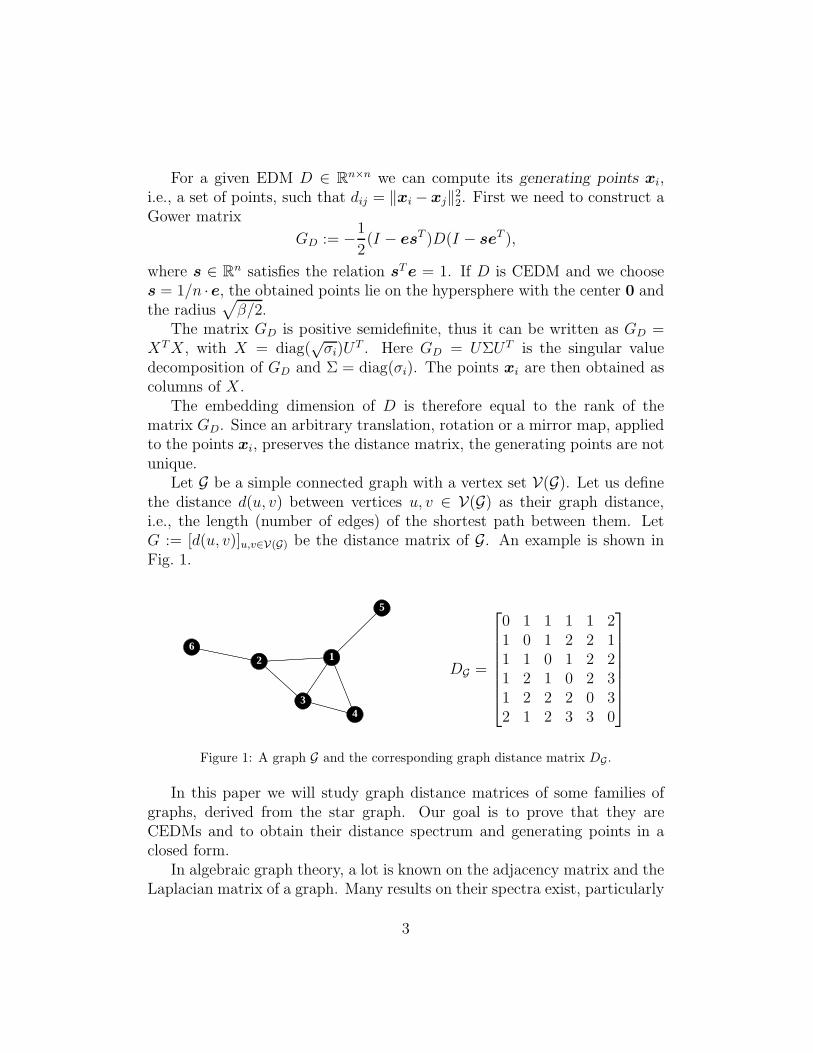
Let G be a simple connected graph with a vertex set V(G). Let us definethe distance d(u, v) between vertices u, v ∈ V(G) as their graph distance,i.e., the length (number of edges) of the shortest path between them. LetG := [d(u, v)]u,v∈V(G) be the distance matrix of G. An example is shown inFig. 1.

12

34

5

6

DG =

0 1 1 1 1 21 0 1 2 2 11 1 0 1 2 21 2 1 0 2 31 2 2 2 0 32 1 2 3 3 0

Figure 1: A graph G and the corresponding graph distance matrix DG .

In this paper we will study graph distance matrices of some families ofgraphs, derived from the star graph. Our goal is to prove that they areCEDMs and to obtain their distance spectrum and generating points in aclosed form.

In algebraic graph theory, a lot is known on the adjacency matrix and theLaplacian matrix of a graph. Many results on their spectra exist, particularly

3

on properties of their largest and smallest eigenvalues (see [4], e.g.). Not muchis known on the graph distance matrix. It could be efficiently computed byDykstra algorithm, e.g. Some results on its structure and its spectrum, theso-called D-spectrum for particular graphs were given in [12, 14].

Similar problems were studied in several papers. Line distance matri-ces (corresponding to paths) were considered in [19, 16], cell matrices (forweighted star graphs) were introduced in [16], distance matrices of weightedtrees were studied in [1, 7], and distance matrices of weighted paths andcycles were analysed in [18].

This paper generalizes and extends some of these results to a broaderfamily of graphs. In this way, a deeper insight into the relation betweengeneral graphs (and networks) and EDM structure is obtained. Hopefully,this will enable a more thorough study of the problem considered.

The structure of the paper is as follows. In the second section we analysethe star graph, k-star graphs and trees in general and prove that their graphdistance matrices are CEDMs. The distance spectrum (D-spectrum) of thestar graph is given in a closed form as well as its generating points. Inthe third section we study properties of circulant matrices that will be animportant tool throughout the paper. The generalizations of the star graph(the wheel, the gear and the helm graph) are analysed in the fourth, the fifthand the sixth section. We prove that their distance matrices are CEDMs.We give the distance spectra of the wheel and the gear graph in a closedform. For the wheel graph we also compute the generating points of thecorresponding distance matrix. The paper is concluded with an example.

2. Graph distance matrices of star and k-star graphs

The star graph Sn, n ≥ 2, is a graph with n− 1 vertices of degree 1, con-nected to a vertex of degree n−1. If we take k star graphs Sm1

,Sm2, . . . ,Smk

,mi ≥ 2, and connect all of their inner vertices, we obtain the so-called k-stargraph. Properties of distance matrices of weighted star and k-star graphswere studied in [16], where it was proven that they are CEDMs.

In this paper we are focusing on graph distances. The distance matrixSn ∈ R

n×n of the star graph Sn is of the form

Sn =

[0 eT

e 2(E − I)

].

4

Bordered matrices of the form

D(α) =

[0 αeT

αe D

]

have been analysed in [23] where the following result has been proven.

Theorem 4. If D is a spherical EDM with radius r, then

(1) D(α) is spherical if and only if α > r2.

(2) D(α) is non-spherical if and only if α = r2.

(3) D(α) is not EDM if and only if α < r2.

One can easily verify that the matrix 2(E − I) is CEDM with the radius

r2 =n− 2

n− 1< 1.

Since Sn = D(1) with D = 2(E − I), the following result is an immediatecorollary of Theorem 4.

Corollary 2. The distance matrix Sn of the star graph Sn is CEDM.

Since Sn has a nice structure, we can give its eigenvalues and the corre-sponding eigenvectors in a closed form.

Proposition 1. The distance matrix Sn of the star graph Sn has exactly onepositive eigenvalue

λ1 = n− 2 +√n2 − 3n+ 3

with the corresponding eigenvector u1 =[2− n +

√n2 − 3n+ 3 eT

]T. The

rest of the eigenpairs are

λi = −2, ui =[0 (ei − e1)

T]T

, i = 2, 3, . . . , n− 1, (1)

and

λn = n− 2−√n2 − 3n+ 3, un =

[2− n−

√n2 − 3n+ 3 eT

]T. (2)

5

Proof. Let us denote

ui =

{ [αi eT

]T, i ∈ {1, n}, e ∈ R

n−1,[0 (ei − e1)

T]T

, i = 2, 3, . . . , n− 1, e1, ei ∈ Rn−1.

One can easily verify that the relation Snui = λiui yields the system ofequations which has solutions (1) and (2).

The coordinates of the generating points of Sn can be found via Gower’sreconstruction. First, let us compute the Gower matrix with s = 1/n e,

GSn= −1

2

(I − 1

nE

)Sn

(I − 1

nE

)= − 1

n2

[1− n eT

e (n + 1)E − n2I

].

In order to find coordinates, we have to compute the eigendecomposition ofthe matrix GSn

.

Theorem 5. The Gower matrix of the matrix Sn ∈ Rn×n has the eigenvalues

1, 1, . . . , 1,1

n, 0 (3)

with the corresponding eigenvectors

wi =

√i

i+1

([0 (en−i − e1)

T]T − 1

i

∑i−1k=1

[0 (en−k − e1)

T]T)

, i ≤ n− 2,√

1n(n−1)

[1− n eT

]T, i = n− 1,

√1n

[1 eT

]T, i = n.

(4)

Proof. Let us define

ui =

{ [0 (en−i − e1)

T]T

, i = 1, 2, . . . , n− 2, e1, en−i ∈ Rn−1,

[αi eT

]T, i ∈ {n− 1, n}, e ∈ R

n−1.(5)

For i = 1, 2, . . . , n− 2, the equation

GSnui = λiui (6)

6

implies λi = 1 and for i ∈ {n − 1, n} the equation (6) yields the system ofequations

1− n

n2(1− αi) = λiαi,

1

n2(1− αi) = λi.

It has the solutions

λn−1 =1

n, αn−1 = 1− n, and λn = 0, αn = 1.

Thus we proved that the matrix GSnhas the eigenvalues (3) with the

corresponding eigenvectors

[0

en−1 − e1

],

[0

en−2 − e1

], . . . ,

[0

e2 − e1

],

[1− ne

],

[1e

].

Now let us orthogonalize the set of vectors (5). By using the Gram-Schmidt orthogonalization we obtain a set {vi}ni=1, where

vi =

[0 (en−i − e1)

T]T − 1

i

∑i−1k=1

[0 (en−k − e1)

T]T

, i ≤ n− 2,[1− n eT

]T, i = n− 1,

[1 eT

]T, i = n.

By using

vTi vi =

i+1i, i = 1, 2, . . . , n− 2,

n(n− 1), i = n− 1,

n, i = n,

this yields an orthonormal set of vectors {wi}ni=1, defined in (4).

Note that since one of the eigenvalues is 0, the embedding dimension ofthe generating points of Sn is r = n− 1.

Now we can give the generating points of Sn in a closed form. Let usdenote Σ = diag(1, 1, . . . , 1, 1/n, 0) ∈ R

n×n, and W = [wi]ni=1. The matrix of

generating points of the distance matrix Sn is by the Gower’s reconstruction

X =√Σ W T =

[w1,w2, . . . ,wn−2,

√1/nwn−1, 0

]T.

The generating points are the rows of the matrix X .

7

Theorem 6. The generating points xi ∈ Rn−1, i = 1, 2, . . . , n, of the graph

distance matrix Sn ∈ Rn×n of the star graph Sn are

xi =

1−n

n√n−1

en−1, i = 1,

−∑n−2

k=11√

k(k+1)ek +

1n√n−1

en−1, i = 2,

√n−i+1n−i+2

en−i+1 −∑n−2

k=n−i+21√

k(k+1)ek +

1n√n−1

en−1, 3 ≤ i ≤ n,

where ei ∈ Rn−1, i = 1, 2, . . . , n.

Proof. It is enough to prove that

‖xi − xj‖2 =

0, i = j,

1, i = 1, j = 2, 3, . . . , n,

2, i = 2, 3, . . . , n, j = i+ 1, i+ 2, . . . , n.

(7)

For i = j the relation (7) obviously holds true. Firstly,

‖x1 − x2‖2 =n−2∑

k=1

1

k(k + 1)+

1

n− 1=

n−2∑

k=1

(1

k− 1

k + 1

)+

1

n− 1= 1.

For i = 1 and 3 ≤ j ≤ n,

x1 − xj = −√

n− j + 1

n− j + 2en−j+1 +

n−2∑

k=n−j+2

1√k(k + 1)

ek −1√n− 1

en−1,

thus

‖x1 − xj‖2 =n− j + 1

n− j + 2+

n−2∑

k=n−j+2

1

k(k + 1)+

1

n− 1= 1.

Similarly, for i = 2 and j = 3, 4, . . . , n,

x2 − xj = −n−j∑

k=1

1√k(k + 1)

ek −√

n− j + 2

n− j + 1en−j+1,

thus

‖x2 − xj‖2 =n−j∑

k=1

1

k(k + 1)+

n− j + 2

n− j + 1=

n− j

n− j + 1+

n− j + 2

n− j + 1= 2.

8

In the last case, i = 3, 4, . . . , n and j = i+ 1, i+ 2, . . . , n,

xi − xj =

√n− i+ 2

n− i+ 1en−i+1 +

n−i∑

k=n−j+2

1√k(k + 1)

ek −√

n− j + 1

n− j + 2en−j+1.

Thus

‖xi − xj‖2 =n− i+ 2

n− i+ 1+

1

n− j + 2− 1

n− i+ 1+

n− j + 1

n− j + 2,

and the proof is completed.

Since the eigenvalues of the matrix Sn were given in a closed form, thisreveals some interesting properties.

Lemma 2. The determinant of the matrix Sn is

det(Sn) = (−1)n−1(n− 1) 2n−2,

and

S−1n =

1

2(n− 1)

[−4(n− 2) 2eT

2e E − (n− 1)I

].

Note that the star graph Sn is a tree on n vertices, i.e., a simple, connectedgraph without cycles. Thus Lemma 2 could be proven via the results from[11], where graph distance matrices of trees were studied.

Although in [1] it was proven that (a matrix weighted) distance matrixof a tree is EDM, let us give a simple proof of this fact.

In [11] it was proven that the distance matrix Tn of a tree on n verticesis nonsingular and has exactly one positive eigenvalue (see [21], e.g.). Itsinverse, T−1

n , is a rank 1 matrix minus half the Laplacian matrix of the tree(see [10]),

(T−1n

)ij=

(2− di)(2− dj)

2(n− 1)+

{12aij , i 6= j,

−12di, i = j,

where di := deg(vi) denotes the degree of the vertex vi and aij is the (i, j)-thelement of the adjacency matrix of the tree (see [21], e.g.).

Let w = 1/(n − 1) (2e− d), where d = [d1, d2, . . . , dn]T . By computing

(T−1n e)i =

∑n

j=1 (T−1n )ij, it can easily be verified that Tnw = e. Each tree Tn

has |E| := n−1 edges. And since dTe = 2 |E|, we obtain wTe = 2/(n−1) >0. Thus, by Theorem 2, the matrix Tn is EDM. Theorem 3 with β = (n−1)/2and s = βw yields the following result.

9

Theorem 7. The distance matrix Tn of a tree Tn is CEDM.

In the second part of this section we will focus on k-star graphs and theirgraph distance matrices. Let Sm1

,Sm2, . . . ,Smk

, k > 1, be star graphs, whichwe connect to form the k-star graph Sm,n, where m := [m1, m2, . . . , mk]

T isthe vector of star graphs sizes and n = mTe is the number of vertices ofSm,n. The graph distance matrix of the k-star graph Sm,n is of the form

Sm,n =

Sm1Bm1,m2

. . . Bm1,mk−1Bm1,mk

Bm2,m1Sm2

. . . Bm2,mk−1Bm2,mk

......

. . ....

...Bmk−1,m1

Bmk−1,m2. . . Smk−1

Bmk−1,mk

Bmk ,m1Bmk ,m2

. . . Bmk ,mk−1Smk

∈ R

n×n,

where Smi∈ R

mi×mi is the graph distance matrix of the star graph Smiand

Bmi,mj=

[1 2eT

2e 3E

]∈ R

mi×mj , i, j = 1, 2, . . . , k.

Now we can prove that Sm,n is EDM.

Theorem 8. The graph distance matrix Sm,n of the k-star graph Sm,n, de-fined by m = [m1, m2, . . . , mk]

T ∈ Nk, mTe = n, is EDM.

Proof. Let us take x =[xT1 ,x

T2 , . . . ,x

Tk

]T, where xi =

[αi uT

i

]T ∈ Rmi ,

such that xTe = 0. We will prove that the product

xTSm,nx =

k∑

j=1

(xTj Smj

xj − xTj Bmj ,mj

xj

)+

k∑

i,j=1

xTi Bmi,mj

xj (8)

is nonpositive.Let us write ui = pi + qi, where pi ∈ span{e} and qi ∈ span{e}⊥. Thus

pi = βie and qTi e = 0. Since

xTj Smj

xj = 2αjβj(mj − 1) + 2β2j (mj − 1)(mj − 2)− 2qT

j qj,

xTi Bmi,mj

xj = αiαj + 2αiβj(mj − 1) + 2αjβi(mi − 1)+

+ 3βiβj(mi − 1)(mj − 1),

10

the product (8) simplifies to

xTSm,nx = −k∑

j=1

(2αjβj(mj − 1) + β2

j (mj − 1)(mj + 1) + 2qTj qj + α2

j

)+

+k∑

i,j=1

(αiαj + 2αiβj(mj − 1) + 2αjβi(mi − 1)+

+ 3βiβj(mi − 1)(mj − 1))

= −k∑

j=1

(2β2

j (mj − 1) + (αj + βj(mj − 1))2 + 2qTj qj

)+

+

k∑

i=1

(αi + 2βi(mi − 1)

) k∑

j=1

(αj + βj(mj − 1)

)+

+

k∑

j=1

βj(mj − 1)

k∑

i=1

(αi + βi(mi − 1)

).

The relation xTe implies

k∑

i=1

(αi + βi(mi − 1)

)= 0,

thus

xTSm,nx = −k∑

j=1

(2β2

j (mj − 1) +(αj + βj(mj − 1)

)2+ 2qT

j qj

).

All of the summands are nonnegative, therefore xTSm,nx ≤ 0. The proof iscompleted.

Now we can prove the following.

Theorem 9. The graph distance matrix Sm,n of the k-star graph Sm,n isCEDM.

Proof. By Theorem 8 the matrix Sm,n is EDM. Thus it is enough to see thatthere exists w ∈ R

n such that Sm,nw = e and wTe > 0.

11

Let us denote w =[wT

1 ,wT2 , . . . ,w

Tk

]T, where wi =

[αi βeT

]T ∈ Rmi

and

αi :=2− k(mi − 1)

k(n− k) + 2(k − 1), β :=

k

k(n− k) + 2(k − 1).

Since

Smiwi =

[β(mi − 1)

(αi + 2β(mi − 2)

)eT

]T,

Bmi,mjwj =

[αj + 2β(mj − 1)

(2αj + 3β(mj − 1)

)eT

]T,

a careful calculation shows that

Smiwi +

k∑

j=1

Bmi,mjwj − Bmi,mi

wi = e,

thus Sm,nw = e. By the fact that

wTe =

k∑

j=1

wTj e =

k∑

j=1

(αj + β(mj − 1)

)= 2β > 0,

Corollary 1 implies that the matrix Sm,n is CEDM.

3. Circulant matrices

A circulant matrix (see [8]) is a special case of a Toeplitz matrix, whereeach row of the matrix is a right cyclic shift of the row above it. They are veryuseful in digital image processing and in applications involving the discreteFourier transform.

A circulant matrix C ∈ Rn×n is generated by its first row (c0, c1, . . . , cn−1).

We will use the notation C = circ(c0, c1, . . . , cn−1).First, let us give a relation between circulant matrices and EDMs.

Theorem 10. Let C = circ(c0, c1, . . . , cn−1) ∈ Rn×n be a nonzero circulant

matrix. The matrix C is EDM if and only if

c0 = 0, cj = cn−j ≥ 0, j = 1, 2, . . . ,⌊n2

⌋, (9)

and

2

⌊n−1

2 ⌋∑

ℓ=1

cℓ cos

(2ℓjπ

n

)+ (−1)j

1 + (−1)n

2cn

2≤ 0, j = 1, 2, . . . , n− 1. (10)

12

Proof. The relations (9) ensure that the matrix C is hollow, symmetric andnonnegative. It is well known that all circulant matrices have the sameeigenvectors, and their eigenvalues are closely related to the fast Fouriertransform. More precisely (see [8], e.g.), the matrix C has eigenvalues

λj+1 =n−1∑

ℓ=0

cℓ ωℓj , j = 0, 1, . . . , n− 1, (11)

and the corresponding eigenvectors are

vj+1 :=[1, ωj, ω

2j , . . . , ω

n−1j

]T, (12)

where ωj := exp(i 2πj/n). Clearly, λ1 =∑n−1

j=0 cj > 0 and the correspondingeigenvector is v1 = e. The symmetry in coefficients ci and the facts thatωn−kj = ω−k

j and

ωkj + ω−k

j = 2 cos

(2kjπ

n

)

transform the eigenvalues (11) to (10). If the obtained eigenvalues λj+1, j =1, 2, . . . , n−1 are nonpositive, the matrix C has only one positive eigenvalue.Thus, by Lemma 1, it is EDM.

In [18], the generating points of EDM C were computed.

Theorem 11. [18, Thm. 3.3] The EDM C ∈ Rn×n is generated by points

xi = [xi,1, xi,2, . . . , xi,n−1]T ∈ R

n−1, i = 1, 2, . . . , n, where

xi,j =

√−λj+1

ncos

(2πj(i−1)

n

), j < n

2,

√−λj+1

2ncos

(2πj(i−1)

n

), j = n

2,

√−λj+1

nsin

(2πj(i−1)

n

), j > n

2,

for j = 1, 2, . . . , n− 1.

Circulant matrices play a large role in the following sections where weconcentrate on some families of graphs that are derived from the star graph.

13

4. Wheel graph

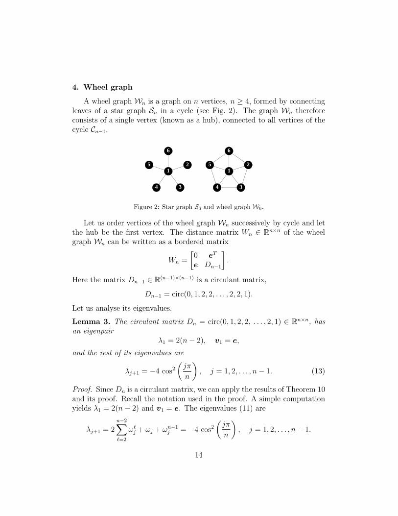
A wheel graph Wn is a graph on n vertices, n ≥ 4, formed by connectingleaves of a star graph Sn in a cycle (see Fig. 2). The graph Wn thereforeconsists of a single vertex (known as a hub), connected to all vertices of thecycle Cn−1.

12

34

5

6

12

34

5

6

Figure 2: Star graph S6 and wheel graph W6.

Let us order vertices of the wheel graph Wn successively by cycle and letthe hub be the first vertex. The distance matrix Wn ∈ R

n×n of the wheelgraph Wn can be written as a bordered matrix

Wn =

[0 eT

e Dn−1

].

Here the matrix Dn−1 ∈ R(n−1)×(n−1) is a circulant matrix,

Dn−1 = circ(0, 1, 2, 2, . . . , 2, 2, 1).

Let us analyse its eigenvalues.

Lemma 3. The circulant matrix Dn = circ(0, 1, 2, 2, . . . , 2, 1) ∈ Rn×n, has

an eigenpairλ1 = 2(n− 2), v1 = e,

and the rest of its eigenvalues are

λj+1 = −4 cos2(jπ

n

), j = 1, 2, . . . , n− 1. (13)

Proof. Since Dn is a circulant matrix, we can apply the results of Theorem 10and its proof. Recall the notation used in the proof. A simple computationyields λ1 = 2(n− 2) and v1 = e. The eigenvalues (11) are

λj+1 = 2n−2∑

ℓ=2

ωℓj + ωj + ωn−1

j = −4 cos2(jπ

n

), j = 1, 2, . . . , n− 1.

14

SinceDn has exactly one positive eigenvalue with the corresponding eigen-vector e, it is by Lemma 1 an EDM.

Corollary 3. The circulant matrix Dn is EDM.

In order to prove that the matrix Wn is EDM, let us recall a lemma,introduced by Fiedler in [6].

Lemma 4. [6, Thm. 2.3] Let A be a symmetric m ×m matrix with eigen-values α, α2, . . ., αm, and let u be a unit eigenvector corresponding to α. LetB be a symmetric n× n matrix with eigenvalues β, β2, . . . , βn, and let v be aunit eigenvector corresponding to β. Then for any ρ, the matrix

C =

[A ρuvT

ρvuT B

]

has eigenvalues α2, α3, . . . , αm, β2, β3, . . . , βn, γ1, γ2, where γ1, γ2 are eigen-values of the matrix [

α ρρ β

].

Now we can prove the following claim.

Lemma 5. The distance matrix Wn of the wheel graph Wn has exactly onepositive eigenvalue.

Proof. By Lemma 3, the matrix Dn−1 has exactly one positive eigenvalue

λ1,Dn−1= 2(n− 3)

with the corresponding eigenvector e. Let us denote its nonpositive eigen-values (13) by λj,Dn−1

, j = 2, 3, . . . , n − 1. Since Wn is a bordered matrix,we can use Lemma 4. If we take ρ =

√n− 1,

A =[0], α = 0, u = 1,

and

B = Dn−1, β = λ1,Dn−1, βj = λj,Dn−1

, j = 2, 3, . . . , n−1, v =1√n− 1

e,

15

Fiedler’s lemma implies that Wn has only one positive eigenvalue

λ1,Wn:= γ1 = n− 3 +

√(n− 4)(n− 2) + n

and nonpositive eigenvalues γ2 = n − 3 −√

(n− 4)(n− 2) + n and λj,Dn−1,

j = 2, 3, . . . , n− 1.

The main result of this section follows.

Theorem 12. The distance matrix Wn of the wheel graph Wn is CEDM.

Proof. By Lemma 5 the distance matrix Wn has exactly one positive eigen-value λ1,Wn

. By Theorems 2 and 3 it is therefore enough to prove that thereexists w ∈ R

n such that Wnw = e and wTe ≥ 0 and that there exist s ∈ R

n

and β ∈ R, such that Wns = βe and sTe = 1.

Let us denote w =[α wT

]T. The equation Wnw = e can be rewritten

as a system of equations

eTw = 1, αe+Dn−1w = e.

By multiplying the second equation by eT , we obtain

α = 1− 1

n− 1eTDn−1w.

Since Dn−1e = 2(n− 3)e, this yields

α =5− n

n− 1, w =

1

n− 1e.

Therefore

wTe = α +wTe =

4

n− 1> 0.

By Corollary 1, the matrix Wn is CEDM, and the proof is completed.

In the last part of this section we give the coordinates of generatingpoints of the wheel matrix Wn. Since Wn is a bordered matrix, the set of itsgenerating points consists of the set of generating points x1,x2, . . . ,xn−1 ofDn−1 that lie on a hypersphere in R

r, where r is an embedding dimension ofDn−1, and a single point

xn = (0, 0, . . . , 0,√1− ‖xi‖2) ∈ R

r+1

16

for arbitrary i ∈ {1, 2, . . . , n− 1}.Since Dn−1 is a circulant EDM, Theorem 11 implies that Dn−1 is gener-

ated by points xi = [xi,1, xi,2, . . . , xi,n−2]T ∈ R

n−2, i = 1, 2, . . . , n− 1, where

xi,j =

2√n−1

cos(

πj

n−1

)cos

(2πj(i−1)

n−1

), j < n−1

2,

0, j = n−12,

− 2√n−1

cos(

πj

n−1

)sin

(2πj(i−1)

n−1

), j > n−1

2,

for j = 1, 2, . . . , n− 2.By Lemma 3, the matrix Dn−1 has an eigenvalue λ1,Dn−1

= 2(n− 3) withthe corresponding eigenvector e. It follows that w = 1/(2(n− 3)) e satisfiesthe relation Dn−1w = e and

wTe =n− 1

2(n− 3).

Thus, by Corollary 1, the generating points of Dn−1 lie on the hyperspherewith the center 0 and the radius R2 = β/2 = (n− 3)/(n− 1). Therefore xn

simplifies toxn = (0, 0, . . . , 0,

√2/(n− 1)) ∈ R

n−1.

Remark 1. Note that the matrix Dn−1 is obtained by using the permutation(1 2 . . . n− 1 n2 3 . . . n 1

)

on the set of generating points x1,x2, . . . ,xn.

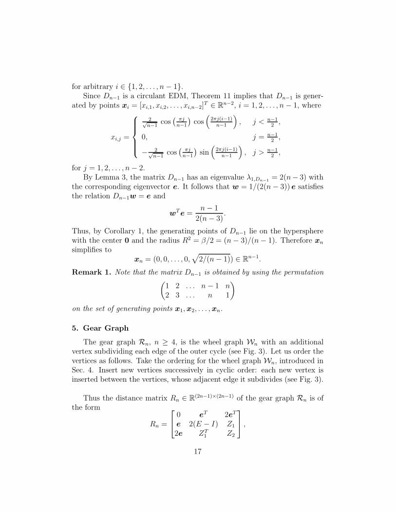
5. Gear Graph

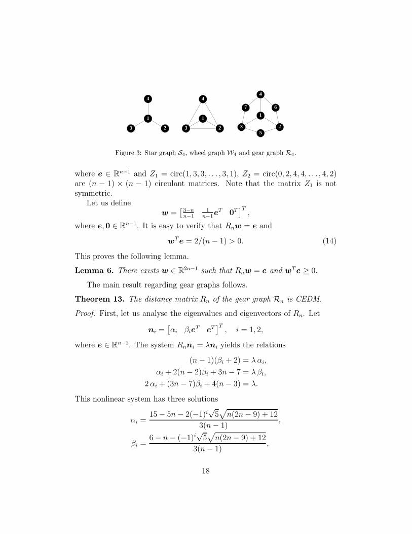
The gear graph Rn, n ≥ 4, is the wheel graph Wn with an additionalvertex subdividing each edge of the outer cycle (see Fig. 3). Let us order thevertices as follows. Take the ordering for the wheel graph Wn, introduced inSec. 4. Insert new vertices successively in cyclic order: each new vertex isinserted between the vertices, whose adjacent edge it subdivides (see Fig. 3).

Thus the distance matrix Rn ∈ R(2n−1)×(2n−1) of the gear graph Rn is of

the form

Rn =

0 eT 2eT

e 2(E − I) Z1

2e ZT1 Z2

,

17

1

23

4

1

23

4

1

23

4

5

67

Figure 3: Star graph S4, wheel graph W4 and gear graph R4.

where e ∈ Rn−1 and Z1 = circ(1, 3, 3, . . . , 3, 1), Z2 = circ(0, 2, 4, 4, . . . , 4, 2)

are (n − 1) × (n − 1) circulant matrices. Note that the matrix Z1 is notsymmetric.

Let us definew =

[3−nn−1

1n−1

eT 0T]T

,

where e, 0 ∈ Rn−1. It is easy to verify that Rnw = e and

wTe = 2/(n− 1) > 0. (14)

This proves the following lemma.

Lemma 6. There exists w ∈ R2n−1 such that Rnw = e and wTe ≥ 0.

The main result regarding gear graphs follows.

Theorem 13. The distance matrix Rn of the gear graph Rn is CEDM.

Proof. First, let us analyse the eigenvalues and eigenvectors of Rn. Let

ni =[αi βie

T eT]T

, i = 1, 2,

where e ∈ Rn−1. The system Rnni = λni yields the relations

(n− 1)(βi + 2) = λαi,

αi + 2(n− 2)βi + 3n− 7 = λ βi,

2αi + (3n− 7)βi + 4(n− 3) = λ.

This nonlinear system has three solutions

αi =15− 5n− 2(−1)i

√5√

n(2n− 9) + 12

3(n− 1),

βi =6− n− (−1)i

√5√n(2n− 9) + 12

3(n− 1),

18

withλi,Rn

= 3n− 8− (−1)i√5√n(2n− 9) + 12, i = 1, 2, (15)

andαi = n− 1, βi = −2, λ = 0. (16)

The eigenvalue λ1,Rnis clearly positive, and a simple calculus confirms that

λ2,Rnis negative. Let xi := ni/‖ni‖, i = 1, 2.

Now let us take a look at the nullspace of Rn. Linearly independentvectors

ni+2 =

{ [1 −(ei + ei+1)

T eTi

]T, i = 1, 2, . . . , n− 2, ei, ei+1 ∈ R

n−1

[1 −(e1 + en−1)

T eTn−1

]T, i = n− 1, e1, en−1 ∈ R

n−1

form a basis of the nullspace. Thus we can construct an orthonormal eigen-vector basis {xi+2}n−1

i=1 that spans the subspace Lin{n3,n4, . . . ,nn+1} andcorresponds to the eigenvalue 0. Note that the solution (16) is included inthis set, since its corresponding eigenvector can be expressed as

[n− 1 −2eT eT

]T=

n−1∑

j=1

nTj+2.

A simple computation shows that the vectors xi, i = 1, 2, . . . , n + 1, aremutually orthogonal.

We need to find the remaining n− 2 eigenvalues. Let us define vectors

ni+n+1 =[0 uT

i vTi

]T, i = 1, 2, . . . , n− 2,

where ui = [u(i)1 , u

(i)2 , . . . , u

(i)n−1]

T , vi = [v(i)1 , v

(i)2 , . . . , v

(i)n−1]

T , and assume that

uTi e = 0, vT

i e = 0. (17)

We would like to obtain an orthogonal eigenvector basis, thus the conditionsnT

i+n+1 xj+2 = 0, i, j = 1, 2, . . . , n− 2, yield the relations

v(i)j =

{u(i)j + u

(i)j+1, j = 1, 2, . . . , n− 2,

u(i)1 + u

(i)n−1, j = n− 1.

(18)

19

The equation Rnni+n+1 = λi+n+1,Rnni+n+1, together with (17), can be rewrit-

ten as

Z1vi = (λi+n+1,Rn+ 2)ui,

ZT1 ui + Z2vi = λi+n+1,Rn

vi. (19)

Note that when we find appropriate solutions vi, the first equation in (19)yields their corresponding counterparts ui.

A simple computation by using (17) and (18) gives

ZT1 ui = 3eTui − 2[u

(i)1 + u

(i)2 , u

(i)2 + u

(i)3 , . . . , u

(i)n−2 + u

(i)n−1, u

(i)n−1 + u

(i)1 ]T

= −2[u(i)1 + u

(i)2 , u

(i)2 + u

(i)3 , . . . , u

(i)n−2 + u

(i)n−1, u

(i)n−1 + u

(i)1 ]T

= −2 vi.

Therefore the relation (19) transforms into the eigenvalue equation for thematrix Z2,

Z2vi = (λi+n+1,Rn+ 2)vi.

The vectors vi are eigenvectors of the matrix Z2 and λi+n+1,Rn= λi,Z2

− 2.But Z2 = 2Dn−1, where the matrix Dn−1 is the circulant matrix, defined

in Lemma 3. By Lemma 3, λ1,Z2= 4(n−3) and the corresponding eigenvector

is e. The rest of the eigenvalues are

λi+1,Z2= −8 cos2

(i π

n− 1

), i = 1, 2, . . . , n− 2. (20)

Hence λi+n+1,Rn= λi+1,Z2

− 2 < 0, i = 1, 2, . . . , n − 2. The solution withthe positive eigenvalue λ1,Z2

and the eigenvector vi = e is not admissibleby assumption (17). Thus we are left with n− 2 negative eigenvalues. Thisconcludes the eigenanalysis of the matrix Rn.

Since the matrix Rn has exactly one positive eigenvalue and by Lemma 6it satisfies the assumptions of Theorem 2, it is EDM.

By (14) and the Corollary 1, the matrix Rn is CEDM. This concludes theproof.

Corollary 4. The matrix Rn has eigenvalues (15), 0, 0, . . . , 0︸ ︷︷ ︸n−1

, and λi+1,Z2−2,

i = 1, 2, . . . , n− 2, defined by (20).

20

6. Helm Graph

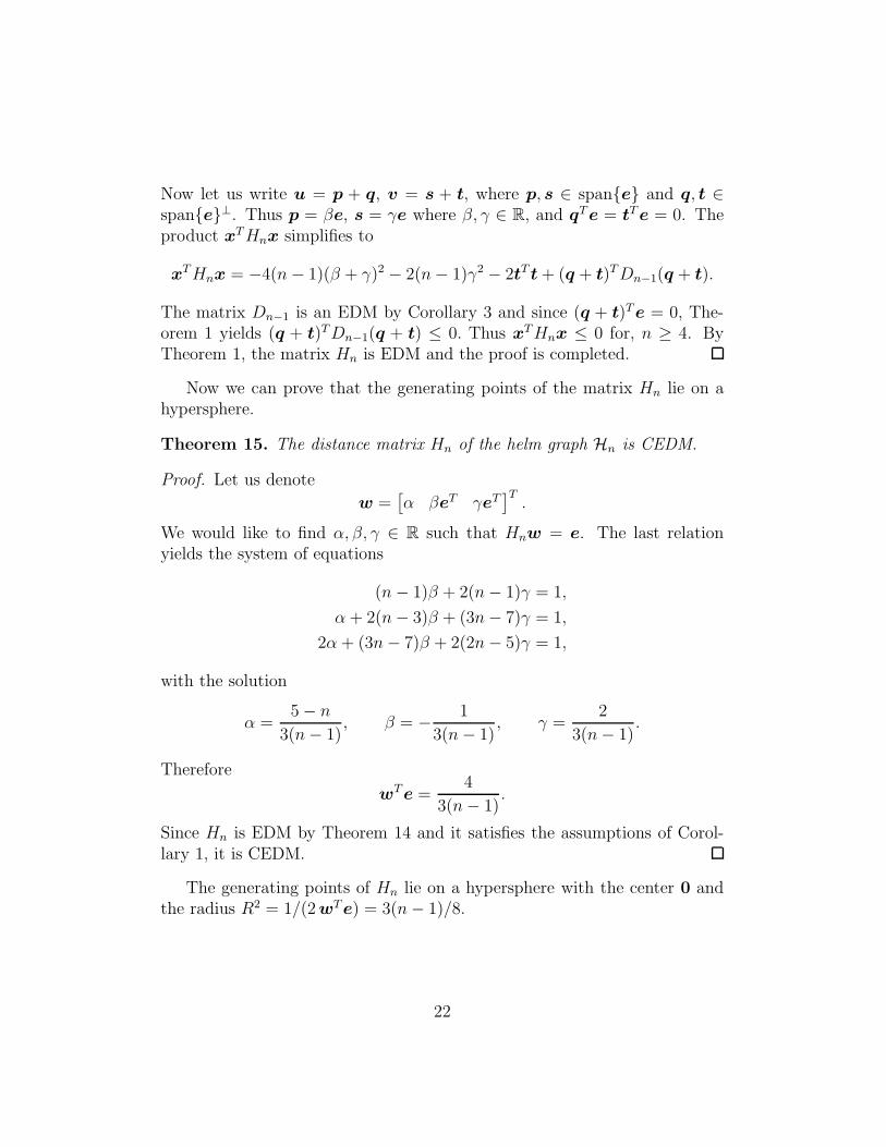
The helm graph Hn, n ≥ 4, is obtained from the wheel graph Wn byconnecting each vertex of the outer cycle Cn−1 to one new vertex. Let us orderits 2n−1 vertices as follows. The first n vertices are ordered as for the wheelgraph Wn. The added n− 1 vertices are ordered successively in cyclic order:each new vertex vi is connected to the vertex vi−n+1, i = n+1, n+2, . . . , 2n−1(see Fig. 4).

1

23

4

1

23

4

123

4

56

7

Figure 4: Star graph S4, wheel graph W4 and helm graph H4.

The distance matrixHn ∈ R(2n−1)×(2n−1) of the helm graphHn is therefore

of the form

Hn =

0 eT 2eT

e Dn−1 Dn−1 + E2e Dn−1 + E Dn−1 + 2(E − I)

,

where e ∈ Rn−1 and Dn−1 ∈ R

(n−1)×(n−1) is the matrix introduced in Sec. 4.First, let us prove that the matrix Hn is EDM.

Theorem 14. The distance matrix Hn of the helm graph Hn is EDM.

Proof. Let us take x =[α uT vT

]T, where α ∈ R and u, v ∈ R

n−1, suchthat xTe = 0. Thus

α = −(uTe + vTe). (21)

Note that Eu = (uTe)e, Ev = (vTe)e, Dn−1e = 2(n − 3)e. A lengthycomputation with the use of (21) shows that

xTHnx = −2((u+ v)Te

)2 − 2(vTv) + (u+ v)TDn−1(u+ v).

21

Now let us write u = p + q, v = s + t, where p, s ∈ span{e} and q, t ∈span{e}⊥. Thus p = βe, s = γe where β, γ ∈ R, and qTe = tTe = 0. Theproduct xTHnx simplifies to

xTHnx = −4(n− 1)(β + γ)2 − 2(n− 1)γ2 − 2tT t+ (q + t)TDn−1(q + t).

The matrix Dn−1 is an EDM by Corollary 3 and since (q + t)Te = 0, The-orem 1 yields (q + t)TDn−1(q + t) ≤ 0. Thus xTHnx ≤ 0 for, n ≥ 4. ByTheorem 1, the matrix Hn is EDM and the proof is completed.

Now we can prove that the generating points of the matrix Hn lie on ahypersphere.

Theorem 15. The distance matrix Hn of the helm graph Hn is CEDM.

Proof. Let us denote

w =[α βeT γeT

]T.

We would like to find α, β, γ ∈ R such that Hnw = e. The last relationyields the system of equations

(n− 1)β + 2(n− 1)γ = 1,

α + 2(n− 3)β + (3n− 7)γ = 1,

2α + (3n− 7)β + 2(2n− 5)γ = 1,

with the solution

α =5− n

3(n− 1), β = − 1

3(n− 1), γ =

2

3(n− 1).

Therefore

wTe =4

3(n− 1).

Since Hn is EDM by Theorem 14 and it satisfies the assumptions of Corol-lary 1, it is CEDM.

The generating points of Hn lie on a hypersphere with the center 0 andthe radius R2 = 1/(2wTe) = 3(n− 1)/8.

22

7. Conclusion

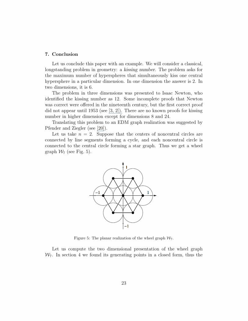
Let us conclude this paper with an example. We will consider a classical,longstanding problem in geometry: a kissing number. The problem asks forthe maximum number of hyperspheres that simultaneously kiss one centralhypersphere in a particular dimension. In one dimension the answer is 2. Intwo dimensions, it is 6.

The problem in three dimensions was presented to Isaac Newton, whoidentified the kissing number as 12. Some incomplete proofs that Newtonwas correct were offered in the nineteenth century, but the first correct proofdid not appear until 1953 (see [3, 2]). There are no known proofs for kissingnumber in higher dimension except for dimensions 8 and 24.

Translating this problem to an EDM graph realization was suggested byPfender and Ziegler (see [20]).

Let us take n = 2. Suppose that the centers of noncentral circles areconnected by line segments forming a cycle, and each noncentral circle isconnected to the central circle forming a star graph. Thus we get a wheelgraph W7 (see Fig. 5).

Figure 5: The planar realization of the wheel graph W7.

Let us compute the two dimensional presentation of the wheel graphW7. In section 4 we found its generating points in a closed form, thus the

23

realization matrix for

W7 =

0 1 1 1 1 1 11 0 1 2 2 2 11 1 0 1 2 2 21 2 1 0 1 2 21 2 2 1 0 1 21 2 2 2 1 0 11 1 2 2 2 1 0

is

X =1

2√6

0 2√3

√3 −

√3 −2

√3 −

√3

√3

0 2 −1 −1 2 −1 −10 0 0 0 0 0 0

0 0 −√3

√3 0 −

√3

√3

0 0 −3 −3 0 3 3

2√2 0 0 0 0 0 0

.

The points xi, i = 1, 2, . . . , 7, are obtained as columns of X . Since a re-alization in R

2 is needed, we take the projection into the x1x5-plane. Theobtained points are x1 = (0, 0), x2 = (1/

√2, 0), x3 = (1/2

√2,−3/2

√6),

x4 = (−1/2√2, 3/2

√6), x5 = (−1/

√2, 0), x6 = (−1/2

√2, 3/2

√6) and

x7 = (1/2√2, 3/2

√6), see Fig. 5.

8. Acknowledgments

This research was funded in part by the European Union, European SocialFund, Operational Programme for Human Resources, Development for thePeriod 2007-2013.

[1] R. Balaji, R. B. Bapat, Block distance matrices, Electron. J. LinearAlgebra 16 (2007) 435–443 (electronic).

[2] P. Brass, W. O. J. Moser, J. Pach, Research problems in discrete geom-etry, Springer, New York, 2005.

[3] J. H. Conway, N. J. A. Sloane, Sphere Packings, Lattices and Groups,3rd Edition, no. 290 in Grundl. Math. Wissen., Springer-Verlag, NewYork, 1999.

24

[4] D. Cvetkovic, P. Rowlinson, S. Simic, An introduction to the theory ofgraph spectra, Vol. 75 of London Mathematical Society Student Texts,Cambridge University Press, Cambridge, 2010.

[5] J. Dattorro, Convex optimization and Euclidean Distance Geometry,Meeboo Publishing, 2009.

[6] M. Fiedler, Eigenvalues of nonnegative symmetric matrices, Linear Al-gebra and Appl. 9 (1974) 119–142.

[7] M. Fiedler, Matrices and graphs in geometry, Vol. 139 of Encyclope-dia of Mathematics and its Applications, Cambridge University Press,Cambridge, 2011.

[8] G. H. Golub, C. F. Van Loan, Matrix computations, 3rd Edition, JohnsHopkins Studies in the Mathematical Sciences, Johns Hopkins Univer-sity Press, Baltimore, MD, 1996.

[9] J. C. Gower, Euclidean distance geometry, Math. Sci. 7 (1) (1982) 1–14.

[10] R. L. Graham, Isometric embeddings of graphs, in Selected topics ingraph theory, 3, Academic Press, San Diego, CA, 1988, pp. 133–150.

[11] R. L. Graham, H. O. Pollak, On the addressing problem for loop switch-ing, Bell System Tech. J. 50 (1971) 2495–2519.

[12] I. Gutman, G. Indulal, On the distance spectra of some graphs, Math-ematical Communications 13 (2008) 123–131.

[13] T. L. Hayden, R. Reams, J. Wells, Methods for constructing distancematrices and the inverse eigenvalue problem, Linear Algebra Appl. 295(1-3) (1999) 97–112.

[14] G. Indulal, Distance spectrum of graph compositions, MathematicalCommunications 2 (2009) 93–100.

[15] G. Jaklic, J. Modic, A note on “Methods for constructing distance ma-trices and the inverse eigenvalue problem”, Linear Algebra Appl., toappear.

[16] G. Jaklic, J. Modic, On properties of cell matrices, Appl. Math. Comput.216 (2010) 2016–2023.

25

[17] G. Jaklic, J. Modic, Inverse eigenvalue problem for Euclidean distancematrices of size 3, submitted, 2011.

[18] G. Jaklic, J. Modic, On Euclidean distance matrices of graphs, submit-ted, 2011.

[19] G. Jaklic, T. Pisanski, M. Randic, On description of biological sequencesby spectral properties of line distance matrices, MATCH Commun.Math. Comput. Chem. 58 (2) (2007) 301–307.

[20] F. Pfender, G. M. Ziegler, Kissing numbers, sphere packings, and someunexpected proofs, Notices Amer. Math. Soc. 51 (8) (2004) 873–883.

[21] S. N. Ruzieh, D. L. Powers, The distance spectrum of the path Pn andthe first distance eigenvector of connected graphs, Linear andMultilinearAlgebra 28 (1-2) (1990) 75–81.

[22] I. J. Schoenberg, Metric spaces and positive definite functions, Trans.Amer. Math. Soc. 44 (3) (1938) 522–536.

[23] P. Tarazaga, J. E. Gallardo, Euclidean Distance Matrices: new charac-terizations and boundary properties, Linear and Multilinear Algebra, 57(7) (2009) 651–658.

[24] P. Tarazaga, T. L. Hayden, J. Wells, Circum-Euclidean distance matri-ces and faces, Linear Algebra Appl. 232 (1996) 77–96.

26