EU Sugar Policy Reform: Quota Reduction and Devaluationaoatools.aua.gr/pilotec/files/bibliography/Witzke_Heckelei2002... · parameters are still excessively simplified for official

EU Sugar Policy Reform: Quota Reduction and Devaluation1

Heinz Peter Witzke and Thomas Heckelei2

University of Bonn

Washington State University

Selected Paper

American Agricultural Economics Association

Long Beach, July 28-31, 2002

Abstract The research presented is part of a larger study aiming at the analysis of reform options for the EU sugar policy regime. This paper focuses on the effects of quota reduction and support price cuts. A thorough theoretical analysis investigates the implications of farm heterogeneity for aggregate supply modeling purposes under the current sugar regime. It can be shown that the treatment of sugar quantities produced under the different quotas and without quota can be treated as different products in an aggregate profit function analysis. Marginal and discrete price and quota effects are derived. Subsequently, the derived behavioral characteristics are implemented in the framework of the agricultural sector model CAPSIM to provide a broader policy evaluation. Preliminary simulation results are presented for the EU at aggregate level.

1 Copyright 2002 by Heinz Peter Witzke and Thomas Heckelei. All rights reserved. Readers may take verbatim copies of this document for non-commercial purposes by any means, provided that this copyright notice appears on all such copies.

2 Heinz Peter Witzke is a Researcher for the European Centre for Agricultural and Resource Economics (EuroCARE), Thomas Heckelei is an Assistant Professor, IMPACT Centre and Department of Agricultural and Resource Economics, Washington State University, USA.. tel: +49-228-732916 or (509) 335-6653; e-mail: [email protected], [email protected].

1 Introduction

The EU sugar market regime has withstood any agricultural policy reform in the last 4

decades despite some effort by agricultural economists pointing at the implied negative

welfare effects (e.g. Koester and Schmitz 1982, Mahler 1994, Bureau et al. 1997). The

“secret” of the production quota based policy was to not touch what seems to worry

politicians more than diminished consumer rents: the budget. But suddenly the invulnerability

of the regime is threatened, mainly by committed tariff preferences and import guarantees to

developing countries. Under the “everything but arms” (EBA) agreement of the EU with the

least developed countries the EU has accepted duty free imports of “everything but arms”,

and what is most important here, this includes sugar. This policy might significantly increase

budget costs of the current sugar market regulation through increased interventions cost and

export subsidies. This in turn could conflict with existing WTO agreements and current

negotiation strategies. Consequently, the European Commission has a strong interest in

evaluating likely consequences of different reform options for the sugar market policy

(European Commission 2001). These options include quota reduction, decreased support

price, and allowing for tradable quotas.

This paper aims at providing some theoretical and preliminary quantitative insights to

the impacts of these options on sugar beet production, income, and welfare at the aggregate

level.3 It is organized as follows: First, a brief overview on the current EU sugar policy is

given. Then, theoretical implications for aggregate modeling of producer behavior under the

quota regime are presented. Farm specific profit maximization models are aggregated

3 Even though CAPSIM simulations will also contribute to the official assessment of the reform options by the Commission, the current specification of the modeling system and the interpretation of options has been solely under the responsibility of the authors. Given that the model is still under construction and that certain policy parameters are still excessively simplified for official use it is very likely that the final CAPSIM results on these options will look different. Therefore, this paper does not allow any inference on the future assessment of the Commission.

1

observing the distribution of efficiency and quota allocation across farms leading to

comparative static results for quota reduction and support price cuts. Based on these

theoretical considerations, the representation of sugar supply behavior in the European Sector

Model CAPSIM is motivated. Subsequently, aggregate results for scenarios with quota

reduction and support price cuts are presented. Finally, conclusions are drawn and research

paths to improve upon the current modeling state and to evaluate additional reform options

are outlined.

2 Common Market Organization (CMO) for Sugar in the EU

2.1 Brief Sketch of Current Measures

The EU's common market organization for sugar (CMO-sugar) is part of the common

agricultural policy (CAP) and was put in place in 1967. It was designed to harmonize the

sugar policy between the member states while keeping producer support at least as high as

with previous national measures. Similar to CMO's for other products, minimum support

prices with an accompanying intervention purchase system were implemented. The internal

market was protected by import tariffs and export refunds. However, in addition to these

typical CMO instruments, a production quota system limited the quantity eligible for price

support through intervention mechanism and thereby the costs of intervention purchases. At

the same time, the quota allocation to member states implied a certain national market share

regardless of efficiency. It was mainly the cost saving nature of the quota system which

allowed the CMO sugar to move basically unchanged through major reforms of the CAP - the

MacSherry reform in 1992 and Agenda 2000.

The quotas allocated to each member state define the sugar quantities that can be sold

in the EU and consequently limit the supply in this market. Production quantities above the

quota, the so called C-sugar, are allowed, but must be sold on the world market. The two

2

types of quota, A and B, are differentiated by the levies applied to cover the cost of export

and production refunds4 of quota sugar:

a basic levy of up to 2% of the intervention price applied to both A- and B-sugar (always

applied since 1990/91)

a variable levy with a maximum of 37.5% of the intervention price applied to B-sugar

(lowest percentage since 1990/91 was 30.4% in 1991/1992)

an additional levy as percentage of the basic and B-sugar levy in case those were not

sufficient to cover the cost (applied 3 times since 1990)

The B-quota in percent of the A-quota differs between member states (highest is

Germany with 30.8% and lowest in Spain with 4.2%). Higher B-quota shares reflect

perceived comparative advantages of certain member states with respect to sugar production

at the time of implementation. They were supposed to allow for an expansion of production at

relatively low product prices. National quota quantities have been nearly unchanged for the

last 20 years. During the same time period there has been only one incidence of intervention

purchases. Apparently, the sugar export with refunds is more attractive for sugar processors.

The member states allocate the quotas to sugar processors, which in turn give delivery

rights to sugar beet producers. The share of A and B quota for producers typically equal the

national shares. Sugar processors are legally bound to pay minimum beet prices to producers,

which calculate as 58% of the intervention price minus the relevant levies. Typically,

producers receive A-quota prices until their individual A-quota is filled, then B-quota prices

apply until the overall quota is exhausted. All remaining quantities delivered are paid

depending on the sugar prices obtained on world markets in the respective marketing year. In

4 The sugar using chemical and pharmaceutical industries receive production refunds to compensate for the additional cost caused by the high sugar prices within the EU.

3

some member states, average pricing schemes are applied (for example on A and B quota

quantities in the Netherlands and Belgium).

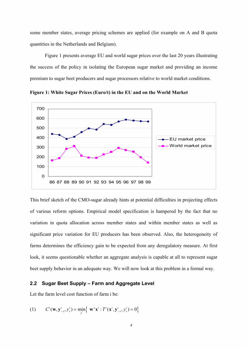
Figure 1 presents average EU and world sugar prices over the last 20 years illustrating

the success of the policy in isolating the European sugar market and providing an income

premium to sugar beet producers and sugar processors relative to world market conditions.

Figure 1: White Sugar Prices (Euro/t) in the EU and on the World Market

0

100

200

300

400

500

600

700

86 87 88 89 90 91 92 93 94 95 96 97 98 99

EU market priceWorld market price

This brief sketch of the CMO-sugar already hints at potential difficulties in projecting effects

of various reform options. Empirical model specification is hampered by the fact that no

variation in quota allocation across member states and within member states as well as

significant price variation for EU producers has been observed. Also, the heterogeneity of

farms determines the efficiency gain to be expected from any deregulatory measure. At first

look, it seems questionable whether an aggregate analysis is capable at all to represent sugar

beet supply behavior in an adequate way. We will now look at this problem in a formal way.

2.2 Sugar Beet Supply – Farm and Aggregate Level

Let the farm level cost function of farm i be:

(1) { }( , , ) min ' : ( , , ) 0− −= =w y w x x yi

i i i i i i i is s s sx

C y T y

4

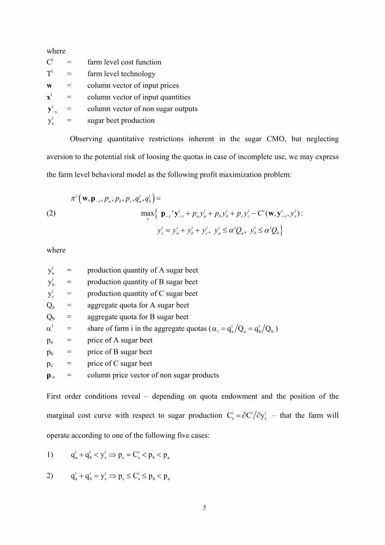
where Ci = farm level cost function Ti = farm level technology w = column vector of input prices xi = column vector of input quantities

is−y = column vector of non sugar outputs

isy = sugar beet production

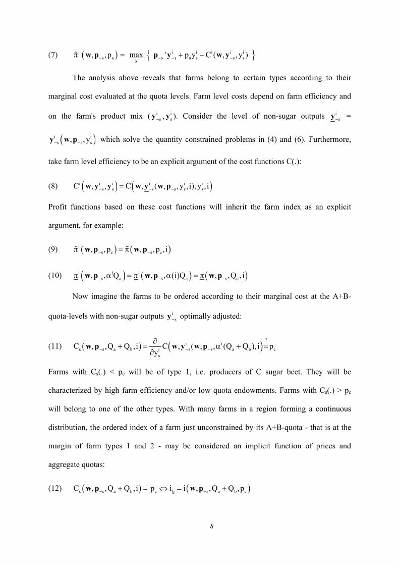
Observing quantitative restrictions inherent in the sugar CMO, but neglecting

aversion to the potential risk of loosing the quotas in case of incomplete use, we may express

the farm level behavioral model as the following profit maximization problem:

(2)

( ){

}

, , , , , ,

max ' ( , , ) :

, ,

−

− − −

=

+ + + −

= + + ≤ ≤

w p

p y w y

i i is a b c a b

i i i i i is s a a b b c c s sy

i i i i i i i is a b c a a b b

p p p q qip y p y p y C y

y y y y y Q y Q

π

α α

where

iay = production quantity of A sugar beet iby = production quantity of B sugar beet icy = production quantity of C sugar beet

Qa = aggregate quota for A sugar beet Qb = aggregate quota for B sugar beet αi = share of farm i in the aggregate quotas ( i i

i a a bq Q q Q= bα = ) pa = price of A sugar beet pb = price of B sugar beet pc = price of C sugar beet p-s = column price vector of non sugar products First order conditions reveal – depending on quota endowment and the position of the

marginal cost curve with respect to sugar production i is yi

sC C= ∂ ∂ – that the farm will

operate according to one of the following five cases:

1) i i i ia b s c s bq q y p C p p+ < ⇒ = < < a

a2) i i i ia b s c s bq q y p C p p+ = ⇒ ≤ ≤ <

5

3) i i i i ia s a b b sq y q q p C p< < + ⇒ = < a

a

a

4) i i is a b sy q p C p= ⇒ ≤ ≤

5) i i is a sy q C p< ⇒ =

These cases are ordered to represent increasing marginal cost and may be depicted

graphically as in figure 2.

Figure 2: Five different farm types in view of the EU sugar CMO

ap

bp

cp

2sy i

sy

(.)C5s (.)C4

s (.)C3s (.)C2

s (.)C1s

4sy5

sy 3sy 1

sy

iaq

ibq

In a certain region we observe several farm types at the same time because quota

endowments and farm efficiency follow a distribution with significant variance. It is quite

clear that the regional aggregate response to changing prices or quota quantities depends on

this distribution and treating each region as homogenous in terms of one of the five farm

types (see, for example, Frandsen et al. 2001) will cause some aggregation error. Before we

develop an aggregate modeling strategy for the evaluation of reform options we first want to

investigate what implications follow from farm heterogeneity. To this end we derive the

aggregate regional profit function for a heterogeneous population of farms.

6

It will be helpful to recognize that each of the above farm types is responsive – at the

margin – to only one sugar related exogenous variable. Type 1, for example, reacts to

marginal changes of the price of C-sugar beet, pc. The other sugar related variables (pa, pb, q , ia

ibq ) only determine which type applies. Unless there are large changes in these variables,

transforming type 1 farms to another one, maximum profit may be determined from

(3) ( ) ( ) ( )

{ } ( ) ( )

i is c a c a b c b

i i i i i i is s c s s s a c a b c b

, , p p p Q p p Q

max ' p y C ( , , y ) p p Q p p Q−

− − −

π + − α + −

+ − + − α + − αy

w p

p y w y

iα =

Sugar beet supply is determined by the price of C-sugar beet pc which enters a price

dependent profit function whereas quotas and prices for A- and B-sugar beet only determine

the additional pure rent income. For farm type 2 the combined A- and B-sugar beet quotas

determine a quantity dependent restricted profit function πi and sugar beet supply:

(4) ( )( ){ }

i i is a b a a b b

i i i i i is s s a b a a b b

, , (Q Q ) p Q p Q

max ' C , , (Q Q ) p Q p Q

−

− − −

π α + + α + α

− α + + α + αy

w p

p y w y

i =

Profit and behavior for farm type 3, which does not fully exploit its B-quota, again follow

from a price dependent profit function iπ :

(5) ( ) ( )

{ } ( )

i is b a b a

i i i i i is s b s s s a b a

, , p p p Q

max ' p y C ( , , y ) p p Q−

− − −

π + −

+ − + − αy

w p

p y w y

α =

The price of B-sugar beet determines behavior whereas quota and price for A-sugar beet are

important for the pure rent income. Farm type 4 is constrained by it’s A-quota such that

behavior and income follow from the solution of:

(6) ( )

{ }

i i is a a a

i i i i is s s a a a

, , Q p Q

max ' C ( , , Q ) p Q

−

− − −

π α + α

− α + αy

w p

p y w y

=

Finally we have farms of type 5 which do not even make full use of their A-quota:

7

(7) ( ) { }i i is a s s a s s s, , p max ' p y C ( , , y )− − −π = + −

yw p p y w yi i i

−

The analysis above reveals that farms belong to certain types according to their

marginal cost evaluated at the quota levels. Farm level costs depend on farm efficiency and

on the farm's product mix ( is−y , i

sy ). Consider the level of non-sugar outputs is−y =

( )is s, , y− −y w p i

s which solve the quantity constrained problems in (4) and (6). Furthermore,

take farm level efficiency to be an explicit argument of the cost functions C(.):

(8) ( ) ( )i i i i i is s s s s sC , , C , ( , , y , i), y , i− − −=w y y w y w p

Profit functions based on these cost functions will inherit the farm index as an explicit

argument, for example:

(9) ( ) (is c s c, , p , , p , i− −π = πw p w p )

(10) ( ) ( ) ( )i iis a s a s a, , Q , , (i)Q , ,Q ,i− −π α = π α = πw p w p w p−

Now imagine the farms to be ordered according to their marginal cost at the A+B-

quota-levels with non-sugar outputs is−y optimally adjusted:

(11) ( ) ( )?

i is s a b s s a bi

s

C , ,Q Q ,i C , ( , , (Q Q ),i py− − −∂

c+ = α +∂

w p w y w p =

Farms with Cs(.) < pc will be of type 1, i.e. producers of C sugar beet. They will be

characterized by high farm efficiency and/or low quota endowments. Farms with Cs(.) > pc

will belong to one of the other types. With many farms in a region forming a continuous

distribution, the ordered index of a farm just unconstrained by its A+B-quota - that is at the

margin of farm types 1 and 2 - may be considered an implicit function of prices and

aggregate quotas:

(12) ( ) ( )s s a b c b s a bC , ,Q Q ,i p i i , ,Q Q ,p− −+ = ⇔ = +w p w p c

8

The number of C-sugar beet producers will decline with rising prices of alternative crops

(∂ib/∂p-s < 0) and with rising aggregate quotas (∂ib/∂Q < 0) but it will increase with rising

prices of C-sugar beet. In an analogous way, we may find the border between the quota

constrained farm type 2 and the unconstrained B-producer type 3 according to equality of

marginal cost, evaluated at the A+B quota levels, with price pb:

(13) ( ) ( )s s a b b b s a bC , ,Q Q ,i p i i , ,Q Q ,p− −+ = ⇔ = +w p w p b

Similarly we find the borders between farm types 3 and 4 and between types 4 and 5:

(14) ( ) ( )s s a b a s aC , ,Q ,i p i i , ,Q ,p− −= ⇔ =w p w p b

(15) ( ) ( )s s a a a s aC , ,Q ,i p i i , ,Q ,p− −= ⇔ =w p w p a

These borders are the final building blocks to calculate the average profit function for a

heterogeneous population of farms by integration over the farm index:

(16)

( )

( )

( )

s

a

a

a

a

b

b

b

s a b c a b

n

s ai

i

s a a ai

i

s b a b ai

i

s a b a a b bi

s c a c a

( , , p , p , p ,Q ,Q )

( , , p , i) f (i) di

( , ,Q ,i) p (i)Q f (i) di

( , , p , i) (p p ) (i)Q f (i) di

( , ,Q Q ,i) p (i)Q p (i)Q f (i) di

( , , p , i) (p p ) (i)Q (

−

−

−

−

−

−

Π

= π

+ π + α

+ π + − α

+ π + + α + α

+ π + − α +

∫

∫

∫

∫

w p

w p

w p

w p

w p

w p( )b

s

i

b c b1n

s1

p p ) (i)Q f (i) d

( , , e) g(e) de−

−

− α

+ π

∫

∫ w p

i

where ib, ib, ia and ia are defined in (12) to (15), ns is the total number of farms endowed and

not endowed with sugar beet quotas, respectively, f(i) is the density of the sugar beet farmers

index. As reflected in (16) Average profit and netput behavioral functions also depend on the

9

farmers without sugar beet quotas which may be simply ordered according to their profit

forming an index “e” with density g(e). In (16) it is assumed for simplicity that their number

n-s is determined by ownership of fixed factors, the distribution of which is considered.

Equally it is assumed that the quota allocation α(i) has been fixed, sometime in the past. To

account for free entry and exit into farming n-s might be considered the price dependent index

of the marginal firm with zero profits (Coyle and Lopez 1987). Total profit and netput supply

follow from multiplication with (ns + n-s).

Taking the derivatives of Π(.) with respect to prices using Leibnitz' rule, for example

pa, illustrates that Hotelling’s Lemma holds for this average profit function as for an

individual firm in spite of the sugar quotas:

(17) ( )

s

a

a

a

b

s a b c a b a s a b c a ba

ns a a

a s a s a a aai

is a a

a s a a a a a aai

i

ai

( , , p , p , p ,Q ,Q ) Y ( , , p , p , p ,Q ,Q )p

i( , ,Q , p )y ( , , p , i) f (i) di ( , , p , i ) f (i )p

i( , ,Q , p )(i)Q f (i) di ( , ,Q ,i ) p (i )Q f (i )p

(i)Q f (i) di

− −

−− −

−−

∂Π =

∂

∂= − π

∂

∂+ α + π + α

∂

+ α

∫

∫

w p w p

w pw p w p

w pw p

a bb

b

ii

a ai 1

(i)Q f (i) di (i)Q f (i) di+ α + α∫ ∫ ∫

The first integral is the production of sugar beet by unconstrained type 5 farmers to which the

A-quota quantities of all other sugar beet farmers are added. The additional effects of pa

through the change in the border ia cancel by construction of the farm index i because for the

farm on the border of farm types 4 and 5:

(18)

( ){ }{ }

s

s s

s a a a a a

s s s a a a a ay

s s a s s s ay ,y

s a a

( , ,Q ,i ) p (i )Q

max ' C( , , (i )Q ,i ) p (i )Q

max ' p y C( , , y , i )

( , , p , i )

−

−

−

− − −

− − −

−

π + α

= − α + α

= + −

= π

w p

p y w y

p y w y

w p

a,

10

because the optimal sugar production ys* = α(ia) Qa for i = ia. Production of "A sugar beet"

falls short of the A quota if there are some type 5 farmers who voluntarily do not fully exploit

their A-quota.

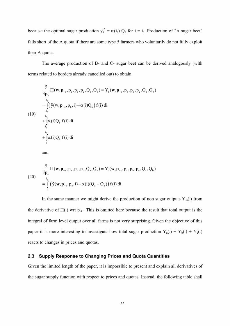
The average production of B- and C- sugar beet can be derived analogously (with

terms related to borders already cancelled out) to obtain

(19)

( )a

b

b

b

b

s a b c a b b s a b c a bb

i

s b ai

i

bi

i

b1

( , , p , p , p ,Q ,Q ) Y ( , , p , p , p ,Q ,Q )p

y( , , p ,i) (i)Q f (i) di

(i)Q f (i) di

(i)Q f (i) di

− −

−

∂Π =

∂

= −α

+ α

+ α

∫

∫

∫

w p w p

w p

and

(20) ( )

b

s a b c a b c s a b c a bc

i

s c a b1

( , , p , p , p ,Q ,Q ) Y ( , , p , p , p ,Q ,Q )p

y( , , p , i) (i)(Q Q ) f (i) di

− −

−

∂Π =

∂

= −α +∫

w p w p

w p

In the same manner we might derive the production of non sugar outputs Y-s(.) from

the derivative of Π(.) wrt p-s . This is omitted here because the result that total output is the

integral of farm level output over all farms is not very surprising. Given the objective of this

paper it is more interesting to investigate how total sugar production Ya(.) + Yb(.) + Yc(.)

reacts to changes in prices and quotas.

2.3 Supply Response to Changing Prices and Quota Quantities

Given the limited length of the paper, it is impossible to present and explain all derivatives of

the sugar supply function with respect to prices and quotas. Instead, the following table shall

11

give an indication of the direction of change when changing exogenous variables in our

context:5

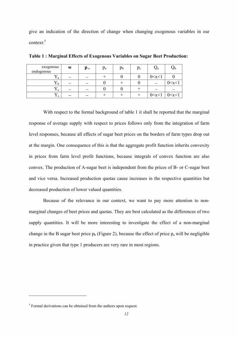
Table 1 : Marginal Effects of Exogenous Variables on Sugar Beet Production:

exogenous endogenous

w p-s pa pb pc Qa Qb

Ya − − + 0 0 0<x<1 0 Yb − − 0 + 0 − 0<x<1 Yc − − 0 0 + − − Ys − − + + + 0<x<1 0<x<1

With respect to the formal background of table 1 it shall be reported that the marginal

response of average supply with respect to prices follows only from the integration of farm

level responses, because all effects of sugar beet prices on the borders of farm types drop out

at the margin. One consequence of this is that the aggregate profit function inherits convexity

in prices from farm level profit functions, because integrals of convex function are also

convex. The production of A-sugar beet is independent from the prices of B- or C-sugar beet

and vice versa. Increased production quotas cause increases in the respective quantities but

decreased production of lower valued quantities.

Because of the relevance in our context, we want to pay more attention to non-

marginal changes of beet prices and quotas. They are best calculated as the differences of two

supply quantities. It will be more interesting to investigate the effect of a non-marginal

change in the B sugar beet price pb (Figure 2), because the effect of price pa will be negligible

in practice given that type 1 producers are very rare in most regions.

5 Formal derivations can be obtained from the authors upon request.

12

Figure 2: Increase of B sugar beet price with farm heterogeneity

ap

cp

isy

aisC

1ai

sC1bi

sC 1sC

iaq i

bia qq +

bisC

2bi

sC2ai

sCsnsC

1bp

2bp

Based on figure 2 and the B-sugar supply function (19), the increase in production of

sugar beet may be calculated as follows:

(21)

( )

( )

( )

2a

1a

1a

2b

2b

1b

2 2 1 1b s a b c a b b s a b c a b

i2

s b ai

i2 1

s b s bi

i1

b s bi

Y ( , , p , p , p ,Q ,Q ) Y ( , , p , p , p ,Q ,Q )

y( , p , p , i) (i)Q f (i) di

y( , , p , i) y( , , p , i) f (i) di

(i)Q y( , , p , i) f (i) di

− −

−

− −

−

−

= −α

+ −

+ α −

∫

∫

∫

w p w p

w

w p w p

w p

For the case of a price increase, ib2>ib

1, because some farms who did not make any use

of their B-quota will use it partially and thus move from type 4 to type 3 (dotted lines in

figure 2). The first integral gives this new production of B-quota beets. The second integral

gives the additional production of B-quota beets on farms belonging to type 3 both before and

after the price change (solid lines in figure 2). Finally a price increase will imply ib2 > ib1,

because some farms who did not before will fully exploit their B quota now, that is they will

13

move from type 3 to type 2 (dashed lines in figure 2). The "old" set of type 2 producers and

the type 1 producers will make full use of their B quota at both prices and hence do not

contribute to the impact of the change in pb. Furthermore, type 5 farmers and a part of type 4

farmers will not change their status for moderate but non-marginal changes. Hence the

production of A-sugar beet and C-sugar beet will not respond at all to moderate price changes

of B sugar beet, just as is case for marginal changes.

Note, that typical aggregate models would not correctly capture the response to

changes in the price of B-sugar beet. If the region were modeled as if it had a marginal cost

curve index of i<ib1, and hence remain in a type 1 or 2 situation, the aggregate response

would incorrectly predicted to be zero. A zero response would also result if the region were

taken to operate as a pure type 4 or 5 farm with farm index i>ia2. If the region were finally

modeled as if it had a farm index of ib1<i< ia

2 the aggregate response would be overestimated.

An improved approach might be to distinguish farm types 1-5 and model their behavior

separately. While being an improvement over a simple representative agent approach it

would miss the endogenous regrouping of farms, which tends to limit the aggregate response.

This is because the type-switching farmers (see the dashed lines in figure 2) are constrained

in their response to a change in pb.

Because a change in the B-quota is a relevant policy option, we will investigate it for

non-marginal changes as well:

14

Figure 3: Decrease of B-Sugar Beet Quota with Farm Heterogeneity

ap

cp

isy

aisC

1bi

sC1bi

sC 1sC

iaq

2bi

sCaisCsn

sC

bp

2bi

sC

i2b

ia qq + i

1bia qq +

Based on figure 3 and the B-Sugar Supply function (19), the effect on the production

of B sugar beet Yb may be calculated as follows:

(22) ( )( )

( ) ( ) ( )

2b

1b

2 11b bb

2 1b b

2 2 1 1b s a b c a b b s a b c a b

i2b s b a

i

i ii2 1 2 1 2 1b b b b b b

1i i

Y ( , , p , p , p ,Q ,Q ) Y ( , , p , p , p ,Q ,Q )

(i)Q y( , , p , i) (i)Q f (i) di

(i) Q Q f (i) di (i) Q Q f (i) di (i) Q Q f (i) di

− −

−

−

= α − −α

+ α − + α − + α −

∫

∫ ∫ ∫

w p w p

w p

With a decrease in the B-quota, both indices for the borders between types 2 and 3 and

between types 1 and 2 will increase. For the graphical presentation we assume that some

farms are of type 2 both before and after the change, i.e. ib1<ib

2<ib1<ib

2. Some former type 3

farmers will become constrained type 2 farmers such that their cut in B-sugar beet production

is less than their quota cut (first integral in (19)). Farms of type 1 will completely substitute

an increase in C sugar beet for former B-sugar beet, whereas some type 2 producers will do

so partially. Consequently the decrease in total sugar production will be clearly less than the

cut in the B-quota.

15

In order to lead over to the simulation exercise presented below, we want to collect

the relevant findings of our theoretical considerations in this respect:

The profit maximization model of the sugar beet producing farm in the EU shows that

each farm operates at one out of 5 possible cases depending on the marginal cost at

the allocated A and B quota levels.

Ordering farms according to their marginal cost at quota levels and incorporating the

farm index as an argument leads to regular profit and derived supply functions for the

average or aggregate farm.

Derived aggregate behavioral functions depend on the separate prices for A-, B, and

C-sugar with distinct effects on other endogenous model variables. This allows (and

requires) treating the corresponding sugar beet quantities in an aggregate analysis as

separate products.

The theoretical analysis provides quantitative ranges for the supply response to

changes in aggregate quota levels (without change in relative allocation across farms).

The behavioral functions depend on an exogenous allocation of sugar beet quotas to

farms. Any change in this allocation implies different quantitative responses to

marginal and discrete variations in exogenous variables.

3 The CAPSIM Model

3.1 Objectives and Overview

The common agricultural policy simulation model (CAPSIM) is being developed to serve as

a speedy and user-friendly policy information system for the European Commission. It is the

16

successor of the medium-term forecasting and simulation model (MFSS, see Witzke,

Verhoog and Zintl 2001).6 The main objectives of the modeling system are

detailed coverage of products and CAP policies

results for the major variables of political interest: agricultural income, market

balances and trade, consumer and budgetary impacts

reliability of results an member state level

user friendliness through ease and speed of operation as well as transparency

The enumeration of these objectives might already make clear that CAPSIM is not a

typical academic tool of analysis. It is designed for quick, repeated policy analysis, requiring

sufficient transparency to allow discussion of model assumptions and scenario specification

with EU officials. Together with the need for a rather disaggregated product list, those

characteristics require some trade-offs that limit the theoretical complexity of the system. The

choices made in model design, however, try to compromise little on the reliability of results.

As the development of CAPSIM from the predecessor MFSS is still incomplete, the

following explanations refer to the intermediate version used for the simulations in this paper.

CAPSIM is currently a comparative static modeling system, driven by a set of synthetic

elasticities. The behavioral functions are based on profit and utility maximization. They are

completed by a set of accounting identities to form a complete set of market balances for

agricultural products as covered by the Economic Accounts for Agriculture (EAA). Market

clearing is either obtained by endogenous trade volumes and policy intervention or through

endogenous prices depending on policy and market characteristics relevant for the specific

commodity. The database mainly integrates different data domains of the Statistical Office of

the European Communities (Eurostat) which comprise market balances, production statistics

6 The description of the modelling system has to be general and informal here for space limitations. For further detailed information see to Witzke, Verhoog, and Zintl (2001), which has been published before the name change to CAPSIM and is the most current available description of the system.

17

and the EAA. Due to missing data and inconsistencies, the database compilation has been

handled by a separate modeling activity (Britz, Wieck, Janson 2002).

3.2 Supply Specification

The supply specification explicitly distinguishes between activity levels and yields of

about 30 production activities. However, yields are taken exogenous to simplify the model

both from a theoretical and practical point of view. It appears that variations in intensity add

little to the aggregate supply response (FAPRI 2000, p. 55).

The underlying profit maximization model endogenously determines activity levels

and input demands. Further characteristics include a feed technology separable from crop

activity levels and the explicit incorporation of land and calves balances. With the exception

of feed demand, input prices and revenues per activity unit drive behavioral functions. The

latter are calculated based upon market prices, price supports, and yields as well as hectare or

livestock premiums. Feed demand functions are conceptually derived from a cost function

and include animal activity levels and feed prices as determining factors.

The underlying optimization model provides an explicit framework for the calibration

of activity and input demand elasticities based on a Maximum Entropy procedure observing

microeconomic conditions in the base year situation. In the intermediate version of CAPSIM

most behavioral functions are expressed in double log form.

3.3 Demand Specification and Market Clearing

The modeling of food demand is modeled based on a utility maximization model

subject to a budget constraint. Consumer prices, total private expenditure, and population

determine derived demands. Again, standard microeconomic conditions are imposed

including full curvature. The specification is derived from a Generalized Leontief cost

function (see Witzke, 2002).

18

For most products, processing and price linkages between producer and consumer

prices are not explicitly modeled. A fixed “marketing margin” applies in these cases. For the

case of oilseeds, potatoes, olives, and “other cereals”, milk, and sugar beet, an explicit

processing model at the EU-level is included. With the exception of the last two products,

processing quantities are determined based upon a behavioral function derived from a profit

maximization hypothesis subject to fixed processing coefficients. Due to the absence of

significant raw product trade in milk and sugar beet, it may be assumed for these products

that basically the complete usable production is also processed. For sugar beet, this is

combined with a constant return to scale assumption for the processing technology leading to

a fixed processing cost.

3.4 Policy Representation

Overall the most important support instrument of the current CAP is the system of

premiums for crop and livestock activities. These premiums have been constrained by

ceilings, again reflecting the overriding importance of budgetary considerations in the EU.

An obligatory set aside rate accompanies the system of premiums. To account for the

counteracting response of voluntary set aside to a change in the obligatory set aside rate, the

latter translates less than proportionally to the effective set aside area in the model. The milk

quota regime is implemented in a standard way. This leads to a divergence of market

revenues and shadow revenues, the latter of which have been specified in view of results in

Barkaoui, Butault, and Guyomard 1997.

Most interesting for this paper is the implementation of sugar policies. According to

section 2.3, A-, B-, and C-sugar beet are treated as separate products with strong supply

response to changes in the respective quotas. Those may be considered as fixed factors in

formal terms. The crucial elasticities will be specified based on an analysis of FADN data,

19

which is not yet finished. To obtain the operational intermediate version we relied on the

following assumptions on some of the required elasticities:

Table 2: Preliminary Specification of Sugar Beet Elasticities:

exogenous endogenous

pa pb pc Qa Qb

Ya 0.005 0 0 0.99 0 Yb 0 0.1 0 −0.2 0.9 Yc 0 0 0.5 −0.2 −0.04

The self-financing character of the sugar market organization has been incorporated in

CAPSIM. Consequently the levies on B-sugar have to finance the export subsidies for A+B-

sugar which are not covered by the basic levy. This accounts for the increase in the producer

price of B-sugar beet after an increase in the world market price of sugar or a decrease in the

sugar quota. As long as they are below international prices, EU market prices proportionally

follow any change in the EU intervention price. Consequently, it is assumed that EU

authorities adjust export subsidies exactly by the amount necessary to bring about this

parallel movement which has been observed in the past even though market prices are usually

somewhat higher than intervention prices.

4 Scenario Specification and Results

4.1 Scenario specification

The chosen simulation year is 2011. The Reference run implies the full implementation of the

Agenda 2000 package (see European Commission 2000 or Witzke, Verhoog, Zintl 2001 for

details).

Administered prices for cereals, beef and raw milk reduction in accordance with

Agenda 2000.

Per-hectare premiums for cereals rise to compensate for the decline in prices, with

little change on the durum wheat premium. Premiums for pulses and oilseeds,

20

however, decline to more or less complete the equalization of payments with those for

cereals. Cattle premiums rise to partly compensate for the drop in intervention prices.

The obligatory set-aside rate is set to 10 %.

Milk quotas rise in line with the Berlin summit decisions.

For sugar we assume one million tons of additional imports into the EU from EBA

beneficiaries which effectively reduces the maximum quantity of subsidized exports

stemming from EU A- and B- sugar beet.

In view of the Commission’s call for proposals we specified the following policy

options:

Option 1: Uniform reduction of all sugar quotas (A+B) by 13%. This turned out

sufficient to not only avoid any intervention purchases but also to dispense with

subsidized exports in spite of the new EBA imports.

Option 2: Reduction of the intervention price from 630 Euro/t to 340 Euro/t. Even

though the resulting intervention price is basically equal to the assumed world market

price (339 Euro), the price decline proved insufficient in this modeling exercise to

make subsidized exports or intervention unnecessary.

4.2 Results

The results are illustrative for the theoretical developments of section 3.

Table 3 : Results on Area Use

Base 1997/99

Reference 2011

Low quota 2011

Low quota - Reference

Low price 2011

Low price - Reference

Soft wheat revenue 1034 1251 1250 -0.1% 1250 0.0% Soft wheat area 13865 14267 14310 0.3% 14265 0.0%

Sugar beet area 2080 2099 1906 -9.2% 2029 -3.3% A sugar beet revenue 3056 3054 3172 3.9% 488 -84.0% A sugar beet area 1457 1473 1295 -12.0% 1456 -1.1% B sugar beet revenue 2136 3020 3195 5.8% 492 -83.7% B sugar beet area 311 323 297 -7.9% 269 -16.5% C sugar beet revenue 270 293 293 0.0% 293 0.0% C sugar beet area 312 303 314 3.4% 303 0.0%

21

Given the small share of sugar beet in crop area (about 2.5%) the effects on other crops are

almost negligible in the two policy scenarios as is visible on the example of soft wheat which

is reproduced in the table. The different responses of sugar beet areas to changes in quotas or

revenues are evidently related to our elasticity assumptions.

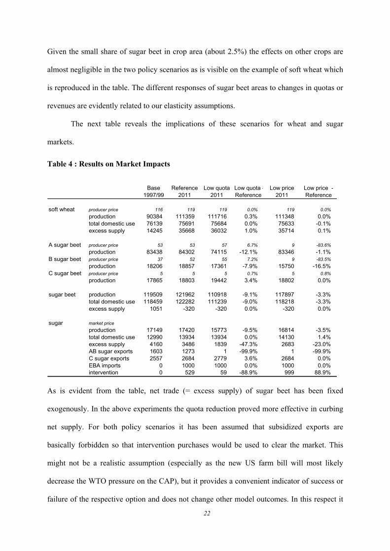
The next table reveals the implications of these scenarios for wheat and sugar

markets.

Table 4 : Results on Market Impacts

Base 1997/99

Reference 2011

Low quota 2011

Low quota -Reference

Low price 2011

Low price - Reference

soft wheat producer price 116 119 119 0.0% 119 0.0% production 90384 111359 111716 0.3% 111348 0.0% total domestic use 76139 75691 75684 0.0% 75633 -0.1% excess supply 14245 35668 36032 1.0% 35714 0.1%

A sugar beet producer price 53 53 57 6.7% 9 -83.6% production 83438 84302 74115 -12.1% 83346 -1.1%

B sugar beet producer price 37 52 55 7.2% 9 -83.5% production 18206 18857 17361 -7.9% 15750 -16.5%

C sugar beet producer price 5 5 5 0.7% 5 0.8% production 17865 18803 19442 3.4% 18802 0.0%

sugar beet production 119509 121962 110918 -9.1% 117897 -3.3% total domestic use 118459 122282 111239 -9.0% 118218 -3.3% excess supply 1051 -320 -320 0.0% -320 0.0%

sugar market priceproduction 17149 17420 15773 -9.5% 16814 -3.5% total domestic use 12990 13934 13934 0.0% 14130 1.4% excess supply 4160 3486 1839 -47.3% 2683 -23.0% AB sugar exports 1603 1273 1 -99.9% 1 -99.9% C sugar exports 2557 2684 2779 3.6% 2684 0.0% EBA imports 0 1000 1000 0.0% 1000 0.0% intervention 0 529 59 -88.9% 999 88.9%

As is evident from the table, net trade (= excess supply) of sugar beet has been fixed

exogenously. In the above experiments the quota reduction proved more effective in curbing

net supply. For both policy scenarios it has been assumed that subsidized exports are

basically forbidden so that intervention purchases would be used to clear the market. This

might not be a realistic assumption (especially as the new US farm bill will most likely

decrease the WTO pressure on the CAP), but it provides a convenient indicator of success or

failure of the respective option and does not change other model outcomes. In this respect it

22

is evident that a quota cut of around 13% would be sufficient to solve the trade related

problems of the EU. This does not hold for the price reduction scenario.

However, in quantitative terms, the supply impact of the price decline does not seem

very realistic. While it is perfectly plausible to assume a fairly low response of A-sugar beet

to the own revenue at the current high prices, it may be questioned that this elasticity remains

low for drastic price reductions such as those considered above. A different functional form

with non-constant elasticities would have most likely changed the results in this respect. This

issue will be addressed in the upcoming weeks, but could not be tackled at the moment.

After completion of the database revision on subsidies, a complete welfare analysis in

terms of producer income, consumer welfare and budgetary (EAGGF) impacts will be added

to the market results above. This will provide a more complete picture as the income effects

and benefits to consumers are of course quite different.

5 Conclusions

This paper has made a number of contributions. In theoretical terms we have

developed the implications of farm heterogeneity for aggregate supply modeling purposes

under the EU quota regime. The derived behavioral characteristics have been implemented in

the framework of the agricultural sector model CAPSIM, for the time being based on

assumed parameters. Contingent upon those, simulation results for the year 2011 have shown

that a moderate quota reduction of 12.5% allows avoiding subsidized exports and/or

intervention purchases, whereas a drastic reduction of prices to world market level is not

sufficient in this respect. Apart from uncertainties with respect to the parameter specification,

the preferability of any one of these options cannot be concluded without consideration of

welfare effects on all involved groups.

Research during the next months will concentrate on econometric estimation at farm

level. This will not only provide firmer empirical ground for the parameter specification

23

under the current quota regime, but also provide the opportunity to investigate changes in the

aggregate supply response, if quotas were allowed to be traded between farms or regions –

another reform option to be considered.

24

References

Barkaoui, A., J.-P. Butault, and H. Guyomard. Mobilité des droits à produire dans l'Union

européenne - Conséquences d'un marché des quotas laitiers à l'échelle régionale,

nationale ou communautaire.” Cahiers d' économie et sociologie rurales (44):6-28,

1997.

Britz, W., C. Wieck, and T. Jansson. “National Framework of the CAPRI – Database: The

CoCo Module.” CAPRI-Working Paper 02-04, University of Bonn and Swedish

Institute for Food and Agricultural Economics (SLI), 2002.

Bureau, J.-Ch., H. Guyomard, L. Morin, and V. Réquillart. “Quota Mobility in the European

Sugar Regime”. European Review of Agricultural Economics 24:1-30, 1997.

Coyle, B.T., and R.E. Lopez. “On Industry Adjustment in Long Run Equilibrium”.

Discussion Paper, University of Manitoba and University of Maryland, 1987.

European Commission. Open Call for Proposals – Study to Assess the Impact of Options for

the Future Reform of the Sugar Common Market Organisation. Agricultural Directorate

General, Brussels, 2001.

European Commission (DG Agri). “CAP Reform Decisions Impact Analysis.” Luxembourg:

Office for Official Publications of the European Communities, 2000.

Frandsen, S.E., H.J. Jensen, W. Yu, and A. Walter-Jørgensen. “Modeling EU Sugar Policy –

A study of policy reform scenarios.” Danish Institute of Agricultural and Fisheries

Economics, SJFI Working Paper no. 13/2001.

Koester, U., and P.M. Schmitz. “The EC Sugar Market Policy and Developing Countries.”

European Review of Agricultural Economics 9:183-204, 1982.

Mahler, P. “Efficiency losses as a result of insufficient structural adjustments due to the EC

sugar regime: The case of Germany.” European Review of Agricultural Economics

21:199-218, 1992.

25

26

Witzke, H.P. “Conceptual framework for the respecification of the demand side in CAPSIM.”

Working Paper, EuroCARE, Bonn, 2002.

Witzke, H.P., D. Verhoog, A. Zintl. “Agricultural Sector Modelling. A new medium-term

forecasting and simulation system (MFSS99).” Research in Official Statistics,

European Commission, 2001.