ETHIOPIA’S FOREST REFERENCE LEVEL SUBMISSION TO THE …

ETHIOPIA’S FOREST REFERENCELEVEL SUBMISSION TO THE

UNFCCC

August 2016

2

1. CONTENTS

1. Contents........................................................................................2

2. Summary: The Proposed FRL.........................................................7

3. Introduction..................................................................................8

4. Scale..............................................................................................9

5. Scope: activities, pools and gases included.................................10

5.1. REDD+ activities in the FRL..............................................................10

5.2. Carbon Pools in the FRL..................................................................11

5.3. Gases in the FRL.............................................................................12

5.4. Forest definition..............................................................................12

5.5. Drivers of Deforestation and Forest Degradation............................14

6. Historical Period..........................................................................16

7. The Ethiopian Biomes..................................................................17

8. The Activity Data assessment process.........................................21

8.1. Ethiopia’s Land Use and Land Cover Map 2013................................21

Image analysis...................................................................................................21

8.2. The Forest/non forest Map..............................................................24

8.3. Forest Change Detection in Ethiopia................................................24

8.4. Step by step Processes of Change detection....................................25

Step-1 Training Data Collection and validation........................................................26

Setp-2 Image classification and post classification editing........................................27

Step 3 Accuracy Assessment and adjusted area estimates.......................................31

Comparison of Activity Data results with data from Global Forest Change..................37

9. Emission Factors: NFI Data Analysis............................................38

9.1. Description of Ethiopia’s Forest and Landscape Inventory..............38

3

Analysis of NFI Data...........................................................................................42

From Strata to Biomes estimates..........................................................................45

Comparison of the NFI Results and Secondary Data Sources....................................50

9.2. Results and Proposed Emission Factors...........................................51

10. Relevant Policies, Plans And Future Changes............................55

11. Proposed Forest Reference Level...............................................56

11.1. Construction approach and proposed Forest Reference Emission

Level for Deforestation and Forest Reference Level for Afforestation.....56

12. Updating Frequency...................................................................59

13. Future Improvements................................................................60

14. References.................................................................................61

Annex.............................................................................................64

Annex I.................................................................................................64

Annex II...............................................................................................65

4

List of Tables

Table 1: Biomes description......................................................................................20

Table 2: Description of the Land Use/Land Cover Classes.........................................22

Table 3: Criteria for image acquisition......................................................................28

Table 4: Inputs needed for the statistical formula which calculates the number of

overall samples for the accuracy assessment..........................................................32

Table 5: Samples distributed in the map classes for verification (collection of

reference data).........................................................................................................32

Table 6: Error matrix of Ethiopia’s forest change map 2000-2013............................33

Table 7: Error matrix as proportion of agreement and disagreements by total

number of samples in each map class......................................................................34

Table 8: Matrix which gives correct classification, omission (under detection) and

commission (over detection) errors expressed in corresponding map area (ha)......34

Table 9: Adjusted Area estimates (thousands of ha).................................................35

Table 10: Adjusted Area estimates of by biomes (ha)...............................................36

Table 11: Description of NFI strata and number of sampling units located in each

stratum.....................................................................................................................39

Table 12: Tree and other vegetation measurements and observations in NFI...........41

Table 13: IPCC ratios for Below Ground Biomass (2006)...........................................43

Table 14: Number of SU analyzed per region............................................................44

Table 15: Number of SU analyzed per Stratum and per Biome.................................44

Table 16: distribution of the plots per Biome and Ecological Zones:.........................49

Table 17: AGB, BGB and DW per hectare per biome.................................................54

Table 18: sampling distribution and sampling intensity comparisons between NFI

strata and biomes.....................................................................................................64

Table 19: Basic Wood Density of Indigenous and Exotic Tree Species in Ethiopia.....65

5

List of Figures

Figure 1: Figure 1: Extent of the forest cover under the current Ethiopia’s forest

definition.................................................................................................................. 13

Figure 2: Land-uses replacing forest over the period 2000-2013 (as % of the total

forest loss over this period)......................................................................................15

Figure 3: Potential vegetation map of Ethiopia.........................................................18

Figure 4: Biomes of Ethiopia.....................................................................................19

Figure 5: Collect Earth interface for determination of forest change........................27

Figure 6: Number of available Landsat archives queried to create a best pixel mosaic

in Google Earth Engine.............................................................................................29

Figure 7: Iterative classification process for change detection.................................30

Figure 8: Map and adjusted area estimates of AD....................................................35

Figure 9: National forest area change detection 2000-2013 by biome.....................37

Figure 10: NFI sample unit per stratum....................................................................40

Figure 11: Carbon Estimated per strata....................................................................45

Figure 12: The average AGB (tC/ha) with their confidence intervals for forest in the 4

biomes is compared between primary (NFI) and secondary (literature and local

studies) data.............................................................................................................50

Figure 13: IPCC 2006 default values. The asterisk identifies the most represented

ecological zones in Ethiopia......................................................................................51

Figure 14: Above ground biomass per biome............................................................52

Figure 15: Below ground biomass per biome............................................................53

Figure 16: Deadwood per biome...............................................................................53

Figure 17: Emission per biome per year....................................................................56

Figure 18: Removals per biome per year..................................................................58

6

Acronyms

AD activity data

AGB above ground biomass

BGB below ground biomass

CGIAR Consultative Group on International Agriculture Research

CSA Central Statistics Authority

DBH diameter at breadth height

EF emission factor

FAO Food and Agriculture Organization of the United Nations

FRL Forest Reference Level

GLWD Global Lakes and Wetlands Database

GHG greenhouse gas

Ht height

IPCC Intergovernmental Panel on Climate Change

LULC land use/land cover

MEFCC Ministry of Environment, Forest and Climate Change

MMU minimum mapping unit

NFI national forest inventory

REDD Reducing emissions from deforestation and forest degradation

RS remote sensing

SU sampling unit

tCo2 eq ton of carbon dioxide equivalent

UNFCCC United Nations Framework for Conventions on Climate Change

WBISPP Wood Biomass Inventory and Strategic Planning Project

WD wood density

7

2. SUMMARY: THE PROPOSED FRL

Ethiopia’s FRL is in the context of receiving results based payments for REDD+

implementation. The FRL includes deforestation and afforestation, AGB, BGB,

deadwood and CO2 emissions; it is national and based on a historical average of

emissions and removals between 2000 and 2013. The Forest Reference Emission

Level for deforestation is: 17,762,406 tCO2 /year; the Forest Reference Level for

afforestation is: 4,907,634.66 tCO2 /year. The choice of construction approach and

historical period is provisional and may change in the future following appropriate

and comprehensive assessment and national circumstances. In this revised version

of the FRL the estimates have been improved by estimating the emission factors

using countrywide data from the National Forest Inventory and taking into account

the revision of the first submission.

8

3. INTRODUCTION

Ethiopia welcomes the invitation to submit a Forest Reference Emission Level (FRL)

on a voluntary basis expressed in Decision 12/CP.17, paragraph 13. This FRL

submission is in the context of results-based payments for the implementation of

reducing emissions from deforestation and forest degradation, and the role of

conservation, sustainable management of forests and enhancement of forest carbon

stocks (REDD+) under the United Nations Framework Convention on Climate

Change (UNFCCC).

Ethiopia has followed the guidance provided by the UNFCCC through the decisions

taken at the Conference of the Parties (CP), notably the modalities for forest

reference emission levels and forest reference level in Decision 12/CP.17 and the

guidelines for submissions of information on reference levels in the Annex of

Decision 12/CP.17. The original FRL submission was made in January 2016. This

revised version includes revisions that were already foreseen in the original (e.g.

national-level emission factors from recently completed NFI) and some clarifications

as a consequence of the technical assessment process over the last 8 months.

At the same time some of the techniques described in the previous version have

been improved, reason why estimates differ.

This submission does not prejudge or modify any of Ethiopia’s Nationally

Determined Contributions or Nationally Appropriate Mitigation Actions pursuant to

the Bali Action Plan.

Ethiopia intends to take a step-wise approach to its national FRL development as

indicated may be useful in Decision 12/CP.17, paragraph 10. As such, the current

FRL reflects the best available information at the time of submission. Its scope and

methodologies applied may be modified if better data becomes available. The

historical period considered and/or the construction approach may be revised.

9

4. SCALE

The Forest Reference Emission Level will cover the national territory of Ethiopia.

Ground inventory data has been collected in the past three years through the

Ethiopia’s National Forest Inventory. The current submission therefore uses national

activity data and emission factors.

10

5. SCOPE: ACTIVITIES, POOLS AND GASES INCLUDED

5.1. REDD+ ACTIVITIES IN THE FRL

This FRL will include the REDD+ activities deforestation and afforestation

(enhancement of forest carbon stocks). Deforestation will be defined as the

conversion of forest land to other land. Forest land is defined by the Ethiopian

forest definition (see related section) and any transition below the thresholds in this

definition will be considered as deforestation (including the transition of forest land

to open woodland). Afforestation is defined as the conversion of other land to forest

land. Afforestation includes restoration of degraded shrubs and woodlands resulting

in a transition above the thresholds in the forest definition.

Forest degradation is defined as the loss of carbon stock in forest land remaining

forest land, and forest enhancement is defined as the enrichment of carbon stock in

forest land remaining forest land (or the opposite of forest degradation). These

activities are not accounted for in the FRL.

Though forest degradation in the REDD+ context is often considered a significant

source of emissions in Ethiopia, due to the lack of accurate, reliable and consistent

data at the national scale, forest degradation is omitted in this FRL. It is Ethiopia’s

intention to gradually account for forest degradation in the future and currently at

local scales different methodologies are being piloted to assess and monitor forest

degradation: the use of radar images is being tested at project scale and the use of

proxy data on fuelwood consumption is being explored. Ethiopia has the desire and

intention to develop a robust methodology to assess forest degradation and

exploring whether successful attempts at the local level may be transferred into a

cost-effective accounting mechanism at the national level.

Ethiopia’s efforts on natural forest restoration and the development of plantations

are expected to result in reduction of forest degradation and deforestation. In

Tigray and some parts of Amhara the cultivation of plantation as woodlot on

farmers’ own land has been able to supply most of the fuelwood needed (Ethiopia

11

REDD+ Secretariat, 2015) which is expected to reduce the pressure on natural

forest.

Displacement of emissions from deforestation to forest degradation is expected to

be minimal. Deforestation is mainly caused by the expansion of agriculture land,

while degradation is mainly driven by collection of fuelwood and charcoal, livestock

grazing, collection of construction wood and illegal logging. Though there is some

overlap between the drivers of deforestation and forest degradation (livestock

grazing and wood collection may eventually result in a conversion from forest to

open woodland), the expectation is that when addressing these drivers a positive

effect will be seen both on deforestation and forest degradation.

5.2. CARBON POOLS IN THE FRL

The carbon pools included in the FRL will be above ground biomass (AGB), below

ground biomass (BGB), and deadwood. The reason for selecting these pools is that

they are expected to be the most significant pools and primary data has been

collected on these pools through the national forest inventory (NFI). The

methodology applied to collect the litter data in the field only includes the depth of

the litter on the plot. This methodology implies to adopt an ad hoc model to

estimate the carbon content in the litter correctly. This model has not been yet

developed. According to some recent articles, the C fraction contained in litter

consist of less than 0,00% of the total carbon stock (Simegn et al., 2014,

Mikrewongel, 2015, Wolde et al., 2014).

With regard to the soil, this may constitute a very large carbon pool in Ethiopian

forests however, little is known about emissions from soil after forest conversion

and data collection in soils is very costly and needs monitoring over an extended

period. For this reason, the soil carbon pool is not included in the FRL.

Ethiopia does not have a recent soil map, a study (Tekalign et al., 1991) indicates

the Organic Carbon (OC) fraction to be between 0 to 3%. Currently there are no

other extensive and complete studies.

12

5.3. GASES IN THE FRL

The proposed FRL only includes CO2 emissions. Non- CO2 emissions would be

expected from burned areas but since Ethiopia is not systematically collecting data

on the occurrence of fires, data on fire occurrence is not thought to be sufficiently

reliable for inclusion in the FRL. Ethiopia reported a burned forest area of 200 ha in

2003, 800 ha in 2006 and 100 ha in 2008 to FAO’s global Forest Resources

Assessment (FRA) in 2015 (FAO, 2015). To evaluate the significance of non- CO2

gases, a calculation is proposed to estimate the likely range of non- CO2 emissions

by calculating annual non- CO2 emissions for a burned area of 100ha of the lowest

biomass forest (biome 1) and for a burned area of 800ha of the highest biomass

forest (biome 4). Associated non- CO2 emissions are accordingly calculated using

equation 2.27 (IPCC 2006), using default emission factors from Table 2.5 (Tropical

forest) and combustion factor values from Table 2.6 (all secondary forest). This

calculation suggests the contribution of non- CO2 to total forest-related emissions is

in the range of 0.1 – 37.000 t CO2 eq for CO, 0.1 – 33.000 t CO2 eq for CH4 and

3000 – 11.000 t CO2 eq for N2O. Therefore the contribution of non CO2 gases is

estimated to be <2% of total annual emissions from forest land in Ethiopia.

5.4. FOREST DEFINITION

In February 2015 Ethiopia adopted a new forest definition (MEF 2015) as follows:

'Land spanning more than 0.5 ha covered by trees (including bamboo) (with a

minimum width of 20m or not more than two‐thirds of its length) attaining a height

of more than 2m and a canopy cover of more than 20% or trees with the potential

to reach these thresholds in situ in due course (Minutes of Forest sector

management, MEFCC, Feb. 2015). Ethiopia is in the process of approving this as its

national legal definition.

This forest definition differs from the definition used for international reporting to

the Global Forest Resources Assessment (FRA) and from the forest definition used

in the NFI which both applied the FAO forest definition with the thresholds of 10%

canopy cover, a 0.5 ha area and a 5 m height.

13

The reason for Ethiopia to change its national forest definition is to better capture

the natural primary state of Ethiopia’s forest vegetation. In specific, the reason for

lowering the tree height from 5 meters to 2 meters is to capture natural forest

vegetation types like the dryland forests, which in its primary state consist of trees

reaching a height of around 2-3 m. The proposed change in forest definition results

in the inclusion of what previously was classified as Ethiopia’s dense woodlands that

have a wider distribution through the country (Figure 1). Commercial agriculture is

expanding mainly on dense woodlands and Ethiopia desires to enable REDD+

incentives for its conservation.

Figure 1: Figure 1: Extent of the forest cover under the current Ethiopia’s

forest definition

14

The reason for increasing the canopy cover threshold from 10% to 20% is to avoid

acceptance of highly degraded forest lands into the forest definition and in this way

provide incentives for protecting quality forest.

This forest definition also differs from the definition used for reporting greenhouse

gas (GHG) emissions and removals from the forestry sector within the framework of

the Clean Development Mechanism (CDM) that was submitted to the UNFCCC

earlier1, which is “A minimum of 0.05 ha of land covered by trees attaining a height

of more than 2m and a canopy cover of more than 20%. The difference is an‟

increase on area threshold. The main reason for increasing the area in for the FRL

is due the limitation of technology for measurement and monitoring to detect

changes in small areas of forest.

Since Ethiopia has improved the data quality on the forest area change assessment

and changed the forest definition, some inconsistencies currently exist between the

emissions and removals from forestry in the FRL and the GHG inventory. However,

the future GHG inventory reporting in the Biennial Update Report (BUR) will use the

improved data and new forest definition and full consistency will be sought when

reporting results in the technical annex to the BUR.

5.5. DRIVERS OF DEFORESTATION AND FOREST DEGRADATION

A comprehensive study was published by Ethiopia’s REDD+ secretariat (2015)

analysing the drivers of deforestation and forest degradation. The study found

deforestation and forest degradation to be driven mainly by free livestock grazing,

fodder use and fuelwood collection/charcoal production in all the regions followed

by farmland expansion, land fires and construction wood harvesting. The underlying

causes of deforestation and degradation based on framework analysis were

identified to be population growth, unsecure land tenure and poor law enforcement.

Free grazing affects the plains and lowland woodlands to the largest extent. The

large-scale investment agricultural schemes – both private ones and state owned

ones - have been significant drivers in Gambella, Benishangul-Gumuz and Afar

1 https://cdm.unfccc.int/DNA/cdf/index.html

15

Regional States. In Ethiopian Somali and Afar Regional States charcoal is produced

by almost all rural households as one of the core livelihood income sources.

The findings of this study are confirmed by the detection of the land-use replacing

Forest after deforestation assessed by Ethiopia’s National Forest Monitoring System

and described under section 6.2

Figure 2: Land-uses replacing forest over the period 2000-2013 (as % of the total forest

loss over this period)

16

6. HISTORICAL PERIOD

The historical period for which forest area change has been assessed is 2000-2013.

This period was selected to assess change because:

The year 2000 is well covered by standard products (Global Land Surveys

(GLS) and most global products) making it easier to connect or compare to

existing imagery and products

data for this period is available from the Global Forest Change (GFC) product,

(Hansen et al., 2013), which is used as a comparison and as a base for the

change analysis.

The period and dates are in line with requirements by FCPF Carbon Fund

Methodological Framework (criterion 11, indicator 11.1 and 11.2)

However, Ethiopia is still exploring whether the emissions and removals over this

period are representative of emissions and removals expected in absence of REDD+

implementation (and thus whether this historical period is representative as a

benchmark against which to assess performance). Tree cover loss estimates from

the Global Forest Change (GFC) product in 2013 suggest an upwards trend in tree

cover loss in Ethiopia. Ethiopia is still exploring and evaluating which FRL

methodology and/or choice of historical period best reflects emissions expected in

the near future in absence of REDD+ implementation.

17

7. THE ETHIOPIAN BIOMES

A potential vegetation map of Ethiopia has been released by Friis and Sebesebe

(2009) and Friis, Demissew and van Breugel (2010). This map divided the Ethiopian

vegetation into 12 major types, 5 of which with 12 subtypes.

The vegetation types are based on the information related to previous literature,

field experience of the authors, as well as on an analysis of the information for

about 1300 species of woody plants in the Flora of Ethiopia and Eritrea. The map is

based on broad field surveys, mainly along the country roads, and on a set of

classification criteria defining the altitudinal and rainfall limits for each of the

vegetation types. The data on altitude used was obtained from the 90x90 meters

resolution digital elevation model provided by the CGIAR-CSI (2008) with a 3 arc

seconds resolution. The monthly total rainfall data with 30 arc seconds resolution is

from WorldClim. The Global Lakes and Wetlands Database (GLWD) was used to

delineate wetlands and lakes, and the AEON river database (average stream

separation of 15 km) was used to define the boundaries of water bodies and related

vegetation types.

18

Figure 3: Potential vegetation map of Ethiopia

The potential vegetation map has been also used as an input to create the strata

map that is the base layer used to design the national Forest and Landscape

Inventory of Ethiopia.

As the Forest and Landscape Inventory is not focused only on forest strata, during

2015 a new aggregation map was proposed to better represent the reliable carbon

stock estimates. Using the 12 vegetation types as input, these have been

aggregated into 5 biomes following expert judgment by Ethiopian botanical

scientists. Based on their knowledge of the vegetation types and their physiology

they have suggested the following aggregation into four biomes with an expected

homogenous carbon contents (Figure 4)

19

This new stratification has been adopted to estimate the carbon content for the FRL

purposes.

Figure 4: Biomes of Ethiopia

20

Table 1: Biomes description

Biomestrata

Stratumname

Vegetation types (Friss and Sebesebe 2009)

1 Acacia-Commiphora

Acacia-Commiphora woodland and bushland (ACB);Acacia wooded grassland (ACB/RV);Desert and semi-desert scrubland (DSS)

2 Combretum-Terminalia

Combretum-Terminalia woodland and woodedgrassland (CTW);Wooded grassland of the Western Gambela region(WGG)

3 DryAfromontane

Dry evergreen Afro-Montane Forest and Grasslandcomplex (DAF) Afro-Alpine vegetation (AA);Ericaceous Belt (EB);

4 MoistAfromontane

Moist Evergreen Afro-Montane Forest (MAF);Transitional Rain Forest (TRF)

5 Other

21

8. THE ACTIVITY DATA ASSESSMENT PROCESS

The activity data for deforestation and afforestation was assessed as average of

annual forest loss and forest gain in hectares in the period 2000-2013. Satellite

imagery was used in combination with sample data from Google Earth observations

to determine the spatial extent of forest and forest area change. The creation of the

forest and forest area change map is explained under section 8.1, 8.2, 8.3 and 8.4

(step 1 and 2). Errors in the map are identified through verification of the map

classification by visual interpretation (section 8.4, step 3). Accordingly the map

area estimates are corrected for systematic error (bias) in the map (resulting in so-

called adjusted area estimates) and confidence intervals are calculated around the

adjusted area estimates as a measure of the random error remaining in the

estimate after removal of the bias (8.4, step 3). The results are then compared

against the Global Forest Change product and a possible explanation for differences

is provided (section 8.5).

8.1. ETHIOPIA’S LAND USE AND LAND COVER MAP 2013

The Ministry of Environment, Forestry and Climate Change (MEFCC) has created a

map of land use/land cover for the year 2013 using a supervised classification of

Landsat data.This map is used to determine the spatial extent of forests in the FRL.

Image analysis

Landsat 8 imagery was acquired from www.glovis.usgs.gov for images with less

than 3% cloud cover data acquisition dates from March 2013 to December 2013.

The land use/land classes were identified and based on past mapping experiences

of the Woody Biomass Inventory Strategic Planning Project (WBISPP, 2004) and the

prevailing ground situation of the country from the forest inventory. Representative

areas of interests (AOIs) were collected for each of the LULC classes using Google

Earth.

Geometric and radiometric corrections were applied to the Landsat images. The

AOIs served as training data and were used to classify the satellite data using the

Maximum Likelihood algorithm. The libraries of radiometric signatures for the

22

Landsat scenes were iteratively edited to harmonize the scenes. The classified

scene maps were mosaicked to form the thematic land cover/land use map for

Ethiopia.

Table 2: Description of the Land Use/Land Cover Classes

LULC Code LULC Name Description 1 Agriculture Arable and fallow land that grow annual crops (wheat,

maize, sorghum, ‘teff’, Cotton etc) or perennial crops (,sugar cane, ‘enset’, coffee and permanent fruit trees)on the small scale or commercial level by rain fed orirrigation schemes

2 Grassland Land covered with the natural growth of graminea andherbaceous vegetation or a land sown with introducedgrass and leguminous for the grazing of livestock.

3 Scrubland Low bushes and stunted trees, mostly spiny eitherdeciduous or evergreen. More than half of the surfaceof the ground is bare of vegetation.

4 Shrubland Land with shrubs/bushes canopy cover ≤ 10% orcombined cover of bush, and shrubs ≤10%. Shrubs andbushes are woody perennial plants, 2 m in height atmaturity in situ.

5 OpenWoodland

Land covered by natural growth of graminea andherbaceous vegetation, with some scattered trees (treecanopy cover less than 3% . it is composed of a canopyof grass wooded ecosystem of Combretum-Terminaliaand Acacia-Commiphora that can both tolerate burningand temporary flooding with the tall grass strata, incase of the former one.

6 DenseWoodland

A continuous stand of trees with a crown density ofbetween 20 - 80%. Mature trees are usually singlestoried, although there may be layered under-stories ofimmature trees, and of bushes, shrubs andgrasses/forbs. Maximum height of the canopy isgenerally not more than 20 meters, althoughemergents may exceed this. Dense woodland has morethan 400 stems per hectare, whilst open woodland hasbetween 150 and 400 stems per hectare.

7 High Forest A relatively continuous cover of trees, which areevergreen or semi-deciduous, only being leafless for ashort period, and then not simultaneously for allspecies. The canopy should preferably have more thanone story." Three categories of high forest isrecognized: Closed: crown cover of the upper stratum

23

LULC Code LULC Name Description exceeds 80 percent; Dense: crown cover of the upperstrata is between 50 to 80 percent; and Open: crowncover of the upper stratum is between 20 to 50percent.

8 Bareland It is land of limited ability to support life and in whichless than one-third of the area covered by vegetation orother cover. It may be constituted by bare exposedrock, Strip mines, quarries and gravel pits. In general,it is an area of thin soil, sand, or rocks. Vegetation, ifpresent, is more widely spaced and scrubby than thatin the Shrub and Brush category. Unusual conditions,such as a heavy rainfall, occasionally result in growth ofa short- lived, more luxuriant plant cover. Wet, non-vegetated barren lands are included in the Non forestedWetland category.

9 Builtup Urban or Built-up Land is comprised of areas ofintensive use with much of the land covered bystructures. Included in this category are cities, towns,villages, strip developments along highways,transportation, power, and communications facilities,and areas such as those occupied by mills, shoppingcenters, industrial and commercial complexes, andinstitutions that may, in some instances, be isolatedfrom urban areas.

10 Afrolpine This vegetation-type is characterized by small trees,shrubs and shrubby herbs at higher altitudes, herbsand tuussock-forming grasses. Typical bushes andshrub species include Erica arborea, E. trimera andHypericum revolutum. Among herbs in this zone arethe giant lobelia Lobelia rhynchopetalum, Kniphofiafoliosa, Bartsia petitiana and various Alchemillaspecies. Festuca, Poa and Agrostis spp. are typicalgrasses.

11 Plantation Broadleaved, conifer or mixed tree species establishedthrough planting and/or deliberate seeding in acommercial scale or woodlots exceeds 0.5ha,. Includescoppice from trees that were originally planted orseeded.

12 Saltpan Dry Salt Flats occurring on the flat-floored bottoms ofinterior desert basins which do not qualify as Wetland.

13 Wetland Wetlands are those areas dominated by wetlandherbaceous vegetation or are non-vegetate where thewater table is at, near, or above the land surface for asignificant part of most years. These wetlands include,brackish and salt marshes and non-vegetated flats andalso freshwater meadows, wet prairies, and open bogs.

24

LULC Code LULC Name Description 14 Bamboo Naturally regenerated/planted forest predominantly

composed of bamboo vegetation, fulfilling the area,canopy cover and height criteria mentioned at number7.

15 Riverine Are forests which fulfill the definition explained in no 7and grow along with the major river banks and spans20m to 50m buffer from the river. Predominantly itconsists of common families of Moraceae,Spidandaceae, mimosaceae etc

16 Water body Area occupied by major rivers of perennial orintermittent (width ≥ 15m), lakes, ponds andreservoirs.

8.2. THE FOREST/NON FOREST MAP

MEFCC considers High forest, Dense Woodland, Bamboo and Riverine as the

category of forest classes of the country. The LULCs classes of 2013 map were ag-

gregated in to two broad categories of forest and non-forest classes based on the

forest definition of Ethiopia, forested areas exceeding 0.5ha, height ≥ 2m and

canopy cover ≥ 20%. The definition is inclusive of the map forest sub-categories:

forest, bamboo, dense woodland, riverine and plantations. The overall accuracy of

the aggregated map is 81%. The user’s and producers accuracy for the aggregated

forest class is 51% and 56%.

8.3. FOREST CHANGE DETECTION IN ETHIOPIA

The activity data for deforestation and afforestation is assessed as average annual

forest loss and average forest gain in hectares in the period 2000-2013.

The proposed approach by Ethiopia follows the GFOI guiding principle 1 for remote

sensing (GFOI, 2014): a series of images are compared for change detection. The

approaches tested for change detection include purely automatic spectral methods

(e.g. IMAD algorithm) and supervised change detection using change training

points/loss and gain (Tewksebury et al. 2015). Post classification change detection

is not a suitable option for Ethiopia because historical land cover maps do not have

sufficient accuracy to derive change. Studies examining post classification change

have shown two forest/non-forest maps can be highly accurate with user's

25

accuracies of about 95%, the user's accuracy of the deforestation class in the

change map is likely to be much lower, indicating that the forest change obtained

by post-classification is inaccurate.

The method chosen was a supervised classification of imagery, in which the user

identifies representative spectral samples for each class in the digital image. The

representative spectral samples are used as a dictionary and the classification

algorithm uses this dictionary to classify all objects/pixels depending on what their

spectral signature resembles most in the dictionary. In the case of change

detection, the object to be classified is a multi-temporal stack of imagery, and the

classes are change (loss and gain) or stable.

The imagery chosen for the exercise is Landsat data2, adapted to forest land cover

detection (FAO & JRC, 2012). The process assessed two mosaics for the year 2000

and 2013, to assess the change occurred in this period. For each year, all available

pixels covering a specified area and date range are collected and corrected for sun-

sensor-target anomalies3. A target day is fixed in order to get the maximum

vegetation cover and least cloud cover as possible. The proximity to this target day,

the pixel temperature and pixel wetness are computed to create a best-pixel

mosaic. The two best pixel mosaics (one for each time period) are finally stacked

into a consistent multi-temporal object. All the data collection, correction and

composition are implemented within Google Earth Engine API.

8.4. STEP BY STEP PROCESSES OF CHANGE DETECTION

The Ethiopian FRL considered two types of land use changes; non-forest land use

change to forest as gain, and forest land use change to the non-forest land use as

loss. Forest area change was adjusted using a stratified random sample, using

visually interpreted high temporal and spatial resolution satellite imagery.

2 The choice is justified by the fact that the Landsat images covers the entire time period, correspond to the

technical requirements, are consistent with the data used for the forest area map and are freely available and

likely to be sustainably available in the future (GFOI, 2014).

3 http://landsat.usgs.gov/Landsat8_Using_Product.php

26

The change detection process included:

1. Training data collection and validation;

2. Image classification and post classification editing;

3. Accuracy assessment and area adjustment.

Step-1 Training Data Collection and validation

Supervised classification dependent on the quality of the training sites (Foody and

Mathur, 2006). In the absence of any reliable spatial data to indicate zones of

change at the national level in Ethiopia, preliminary training dataset was generated

automatically from the Global Forest Change product 2013 (GFC, Hansen et al.,

2013). In order to reduce inclusion of potentially false detection in the training

dataset, the GFC product was down-sampled to a 3x3 pixel kernel. The resulting

product was randomly sampled with 300 points for each of the 2 classes (loss and

gain). Points for loss and gains were carefully assessed through a visual assessment

using a times series of Landsat images and vegetation indices and very high

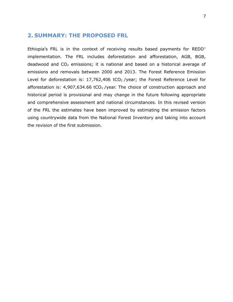
resolution imagery available in the Google Earth, Bing Maps, and Here maps, all

assessed using the Collect Earth interface. Points with a high level of classification

confidence, assigned by the technicians, were used for as the training dataset for

the supervised classification.

27

Figure 5: Collect Earth interface for

determination of forest change

Setp-2 Image classification and post classification editing

Sets of criteria that assist for the filtering and acquisition of Landsat images such as

date of acquisition, date and year range, month of image acquisition and target day

that controls phenology and cloud cover were set by national experts and

incorporated into Google Earth Engine API (specifications are shown in the table 3).

Based on the selection and filtering criteria, GEE-API filtered through the available

Landsat imagery to composite a best pixel mosaic. To use specific bands of Landsat

images and normalize different band naming between Landsat 5, 7 and 8

normalization function was implemented under GEE-API. A function to correct for

latitudinal components of sun-sensor of target geometry was used from

landsat.usgs.gov/Landsat8_Using_Product.php. This function further produces

weighted pixel based on the user specified day of the year, reflectance values of

band ratios, pixel temperature and wetness. To correct longitude and latitudes,

solar elevation angel and radiometric characteristics of each pixel was implemented

using the information obtained from metadata of acquired images.

28

No Criteria Decisions

1 Path and Row To consider the Landsat paths between 162 to 172 and Rowbetween 50 and 58

2 Extent of dates for eachtime period (2000 to 2013)

Start date for initial period in the year of 1997-01-01 to 2003-12-31 and range for the time period two Start date 2010-01001and 2015-03-31

3 Target day , the time withless cloud and mostvegetation

Start Julian day 330th day of the year/November to end of 60thday of the year /February

4 Cloud cover Maximum 90%

Table 3: Criteria for image acquisition

Using the quality function, each band of images from multiple temporal initial and

final time of change assessment were mosaicked. Single images for each time

periods were created using the same script and composited into a multi-temporal

stack for detection of change between the two time periods (figure 6).

The classification process consists of compiling the spectral signature for all the

training points, creating a model from this spectral library and applying the model

to the entire imagery. Two classifiers have been tested, the Classification and

Regression Trees (CART) algorithm (Breiman et al, 1984) and the RandomForest

(RF) algorithm (Breiman, 2001).

The validated training points were used at the national scale to train and directly

classify loss and gain from the mosaicked Landsat images. After a first run of

classification is completed, the training dataset can be improved by visually

assessing zones of false change (i.e stable areas classified as change) and missed

changes (i.e change classified as stable). Examples of potentially incorrect

classifications include agricultural area with strong greenness variations or shadows

29

due to elevation, which could be mistaken for false change and areas with known

deforestation classified as stable. The training sites are added on the misclassified

locations for the correct class. The new sites were entered in the spectral library

with appropriate labelling. Classification was iteratively improved by adding more

points of gain, loss and stable (figure 7). The outputs from the two algorithms were

visually compared and the RF classification was considered superior and used as the

result. The processing chain, from classification of the change, iterative

improvement of the training data, and export of the results was performed.

Figure 6: Number of available Landsat archives queried to create a best pixel mosaic in

Google Earth Engine.

30

Figure 7: Iterative classification process for change detection.

Once the iteration process is determined to have no further improvements to the

31

classification the results can be exported. The exported result from the GEE-API

was filtered to only include loss or gains in clumps of 5 pixels to match the national

minimum mapping unit of forest, 0.5 hectares. The 2013 land cover map was used

to filter false loss by eliminating loss detected on forest and false gain by

eliminating gain detected on non-forest. Manual editing was implemented to

improve the change detection product by delineating false and missed changes

using the Landsat composite image of 2000 and high-resolution imagery for 2013

from Google Earth. An accuracy assessment of the change was finally produced to

estimate the reliability of the change measured (FAO, 2015), produce corrected

estimates of change and confidence intervals around those estimates.

Step 3 Accuracy Assessment and adjusted area estimates

According to IPCC it is good practice for countries to produce emission estimates

which: 1) neither over-nor underestimate actual emissions as far as can be judged,

introducing a systematic error (or bias), and 2) reduce uncertainties as far as

practicable given national circumstances. It is also good practice to quantify

uncertainties and report them in a transparent manner. For emission estimates from

deforestation and removal estimates from afforestation/reforestation, Ethiopia has

assessed forest area loss and forest area gain creating a wall-to-wall forest change

map. This estimation has four classes: forest loss, forest gain, stable forest and

stable non-forest for the period 2000-2013. All surface estimations contains errors,

most of which tend to be systematic (bias). Ethiopia has provided an estimate of

forest loss and forest gain (and forest cover) which is corrected for the map bias.

Classification errors were identified by collecting sample point data. The sample

data verifies whether the classification is correct or incorrect at the location of the

sample points. This information is summarized in an error matrix and the matrix is

used to correct the areas per class (forest loss, gain, stable forest and stable non-

forest) for the map bias resulting in new area estimates, referred to as adjusted

area estimates. To quantify and report uncertainty, Ethiopia also calculates and

reports on confidence intervals around the adjusted area estimates, which provide

an indication of the precision of the estimate. Precision gives a description of

32

random errors or variability. Large confidence intervals indicate a large statistical

variability of the population. The process of correcting the map for bias is referred

to as accuracy assessment.

The required overall number of samples which was calculated using the Olofsson et

al. methodology (2014) adopting the following assumptions, using conservative

user inputs to have a cost effective and robust sample size:

Table 4: Inputs needed for the statistical formula which calculates the number of overall

samples for the accuracy assessment

Input values selected by Ethiopia

Target standard error 0.01

Expected user’s accuracy forest loss 0.5

Expected user’s accuracy forest gain 0.5

Expected user’s accuracy stable forest 0.9

Expected user’s accuracy stable non-forest 0.9

The overall number of samples needed for the accuracy assessment are distributed

over the four map classes as follows: a minimum of 50 samples were allocated to

the “rare” map classes (classes covering a relatively small area) of forest loss and

forest gain. The remaining samples are distributed proportionally based on the

extent of the classes stable forest and stable non-forest.

Table 5: Samples distributed in the map classes for verification (collection of reference

data)

Classes Sample points per map class

Forest loss 84

Forest gain 97

Stable forest 790

Stable non-forest 1013

Ethiopia has collected reference sample data to check whether the map classifica-

tion was correct at the location of the sample point. The sample data is collected by

33

visual interpretation of the point using a time series of very high resolution imagery

and Landsat imagery. The visual interpretation of sample points is referred to as

“reference data”. Only points where the users had high confidence of the classifica-

tion were used, therefore the total number of reference points used in the area esti-

mation is 1984 samples.

An error matrix was used to compare the map classes against the reference data.

The overall accuracy of the map is calculated by dividing the samples where the

map and reference data agree (the bold sample counts in diagonal) divided by the

total number of samples (sum of sample counts in all cells in the matrix)..

Table 6: Error matrix of Ethiopia’s forest change map 2000-2013.

2000-2013 Classes Reference

FL FG SF SNF Total UA

Map

data Forest Loss (FL) 20 2 12 50 84 24%

Forest Gain (FG) 2 17 59 19 97 18%

Stable Forest (SF) 7 5 523 255 790 66%

Stable Non Forest (SNF) 10 1 83 919 1013 91%

Total 39 25 677 1243 1984Producer's Accuracy (PA) 51% 68% 77% 74% OA 75%

FL= Forest Loss , FG= Forest Gain, SF= Stable Forest, SNF= Stable Non Forest, UA= Users Accuracy

In the error matrix, the rows provide information on the ‘over-detections’ (commis-

sion errors) by the map of a certain class, e.g. for the total of 84 samples checked

in the forest loss class in the map, 64 samples were over detected. The commission

errors for loss was when the map identified the sample as loss but the reference

data identified the sample as forest gain (2 samples), stable forest (12 samples),

and stable non-forest (50 samples). The columns in the error matrix provide infor-

mation on the ‘under-detections’ (omission errors), e.g. out of the 39 reference

data points classified as forest loss, the map missed or under-detected 19 samples

as being forest loss. The next steps will identify these under- and over-detections

(bias) in terms of hectares and correct the map area for the commission and omis-

sion errors by calculating adjusted area estimates.

To convert the sample counts into areas by which the map area per class can be

corrected, we first need to convert the absolute sample counts into proportions of

34

the total amount of samples per map class. E.g. for forest loss 20 out of 84 samples

are in agreement which equals to a proportion of 0.24, 2/84= 0.02 was forest gain,

12/84 = 0.14 was stable forest and 50/84= 0.60 was stable non-forest.

Table 7: Error matrix as proportion of agreement and disagreements by total number of

samples in each map class

FL= Forest Loss , FG= Forest Gain, SF= Stable Forest, SNF= Stable Non Forest

In order to obtain the adjusted area, first the map area was calculated multiplyingproportional error matrix of the corresponding rows in the matrix (Table 8) multi-plied by the map areas per class (Table 9) .The result of this multiplication is shownin Table 10

Table 8: Matrix which gives correct classification, omission (under detection) and

commission (over detection) errors expressed in corresponding map area (ha)

FL= Forest Loss, FG= Forest Gain, SF= Stable Forest, SNF= Stable Non Forest

The adjusted area estimates are obtained by the map area minus the over-

detections (commission errors) plus the under-detections (omission errors). E.g.

the adjusted area of forest loss is calculated by 372,188 ha – 88,616 ha – 53,170

ha– 221,540 ha + 824 ha + 907,955 ha = 1,192, 559 ha.

The 95% confidence interval for the adjusted areas are calculated by multiplying

1.96 by the standard error of the area estimate. The standard error of the area

35

estimate is calculated using formula 11 in Olofsson et al 2014. The results are

displayed in the table below:

Table 9: Adjusted Area estimates (thousands of ha).

The results from the accuracy assessment for forest loss for the period 2000 to

2013 is 1,193,000 ha +/- 579,000 ha and for forest gain is 246,000 ha +/- 216,000

ha. The annual forest loss is approximately 92,000 ha/year and annual forest gain

of approximately 19,000 ha/year. This estimate is used as the activity data (see

Figure 8).

Figure 8: Map and adjusted area estimates of AD

Classes

Forest loss 1,193 +/- 579 49%

Forest gain 246 +/- 216 88%

Stable Forest 22,195 +/- 1,716 8%

Stable Non forest 90,780 +/- 1,795 2%

Adjusted area (thousands of ha)

Confidence interval (thousands of ha)

Confidence interval (% of adjusted area)

36

The forest change map has also been overlaid with a map of biomes to divide the

forest loss, gain and forest cover estimates by biome. Forest loss and gain per

biome is used for the calculation of emissions and removals. The gain and loss per

biome is obtained by multiplying the loss/gain/forest areas in each biome by the

overall correction in the map, e.g. forest loss per biome is multiplied by a factor

1,192,55/372,18= 3.18. (Table 10 and figure 9) The relatively high annual forest

area gain in the Dry Afromontane biome gives some evidence that Ethiopia is

already implementing several mitigating actions which aim to restore forest

resources. The on-going mitigation actions reducing emissions are watershed

management, agricultural intensification, trees on farm for fuelwood, declining

livestock (due to stall-feeding, diseases, lack of own fodder and livestock raids),

non-wood and alternative energy sources, and controlled migration.

Table 10: Adjusted Area estimates of by biomes (ha)

FL= Forest Loss , FG= Forest Gain, SF= Stable Forest, SNF= Stable Non Forest

BiomeAdjusted area (thousands of ha)

Forest loss Forest gain

Acacia-Commiphora 194 30

Combretum-Terminalia 712 8

Dry Afromontane 66 179

Moist Afromontane 206 29

14 0.8

Grand Total 1,193 246

Other Biome

37

Figure 9: National forest area change detection 2000-2013 by biome.

Comparison of Activity Data results with data from Global Forest

Change

The average annual loss of 92,000 ha/year over the period 2000-2013 found by the

AD analysis is considerably higher than the tree cover loss found by the Global

Forest Change product, i.e. around 3 times higher. The tree cover loss found by the

Global Forest Product is not very different from the “raw” numbers in the map

before the map bias correction. This difference is explained by the considerable

correction of the area of change in the map for map bias. Remoting sensing is

known to have difficulties detecting dry deciduous forest, especially when on sandy

soils with high reflectance (Bodart et al., 2013). Both the forest loss map created by

Ethiopia and the Global Forest Change map reflect this systematic error therefore

systematically underestimating (dry) forests, and both losses and gains in these

forests.

38

9. EMISSION FACTORS: NFI DATA ANALYSIS

9.1. DESCRIPTION OF ETHIOPIA’S FOREST AND LANDSCAPEINVENTORY

Ethiopia has designed a National Forest and Landscape Inventory since March 2014,

as a Technical Cooperation Programme (TCP) project with FAO. The collection of plot

inventory data has been finalized and a complete data analysis is in course. The

selection and implementation of an appropriate sampling design to collect raw

forest data determines the output of forest information that will be used for various

kinds of decision making processes. The sample design, together with data

collection procedures plays a crucial role in determining the accuracy and the

quality of information from the field. Hence, the NFI of Ethiopia took great

emphasis to craft a suitable forest inventory sampling design that fits the country’s

situation and need of forest information.

After a series of consultations with stakeholders, it was agreed to employ stratified

systematic sampling with reasonable sampling intensities on the respective strata

according to the potential of vegetation they possessed. The NFI uses a

stratification based on Agro ecological Zones of Ethiopia with three dimensional

factors (Altitude, Temperature and Rain fall) together with the land use/land cover

map of WBISPP 2004 and the Potential Vegetation Atlas of Ethiopia (Feriis and

Sebsebe, 2009). The corresponding properties and the number of sampling units

per stratum are described further.

According to the importance of the carbon stock in the strata types (Table 11), the

sampling distances were determined and the plot coordinates were generated using

grid generator. Accordingly, within the grid resolution of 1/4 x 1/4 degree square

and triangular combination grids plots coordinates were generated in the Stratum I,

while a ½ x ½ degree square and triangular combination grids were used for Strata

II and IV, ½ x ½ degree square grid for Stratum III, and a 1x1 degree square grid

in Stratum V, resulting in a total of 631 Sampling Units (SU).

39

Table 11: Description of NFI strata and number of sampling units located in each stratum

Stratum Description Sampling unitsI Comprises natural forest, plantation and Bamboo,

that are found within the altitude range of 2300

to 3200 m.a.s.l.

107

II Comprises of the North and South Eastern part of

the woodland mainly Acacia Commiphora

woodland of Somali, SNNPRs and Afar regions

135

III Comprises mainly the woodland ecosystem found

in the North and South Western woodland parts

where Combretum-Terminalia woodland is

dominant

137

IV This stratum is commonly known as other land

stratum where human activities are dominated

and patches of evergreen Afromontain forest

exist, mostly in the middle altitudes of Ethiopia

(1500 to 2500 m.a.s.l.)

232

IV This stratum refers to the desert and arid pats of

Ethiopia where the elevation range is found below

500 m.a.s.l. and characterized by arid and semi-

arid scrublands.

20

40

Figure 10: NFI sample unit per stratum

In the NFI, data was collected in the field through observations and measurements

at different levels: within the limits of the sampling units (SU) and in smaller

subunits within each SU, and Land Use/Cover Sections (LUCSs). A sampling unit

consists of four subunits (sample plots) that can be divided into LULC. Trees and

stumps in the entire plot area have been recorded and small trees (in forest) and

saplings were recorded in smaller subplots (see the table below).

41

Data collection level

Measurements and observations

Forest

Other WoodedLands and

Woodlots (0.2-0.5ha)

Other lands

SU (samplingunit)

- Localisation and access to SU

- Size: 1000 m x 1000 m (1 km2)

Plot

- Measurement oftrees withDbh ≥ 20 cm

- Size: 250 m x 20

(5000 m2)

- Measurement of trees withDbh ≥ 10 cm

CircularSubplot

- Count of trees with Dbh < 10cm andheight ≥ 1.30m, by species

None

RectangularSubplot Measurement

of trees with10cm ≤ Dbh< 20cm

None None

- Shrubs, bushes (count or measurementby species)

None

- Presence or abundance or count ofindicator plant species, NWFP

Size 20m x 10m

- Indicator plantspecies

FallenDeadwoodTransect

- Measurements of fallen deadwood branches (diameter≥ 2.5 cm)

Size: 20 m

LandUse/CoverSection(LUCS)

- Land Use/Cover class

- General information related to the area (designation, landtenure…)

- Vegetation cover (trees, shrubs, grass)

(- Environmental problems, fires, erosion, grazing activities)

- Stand structure and management:harvesting, silviculture, managementplan...

- Human-induced disturbances

- Cropmanagementpractices

Table 12: Tree and other vegetation measurements and observations in NFI.

42

Analysis of NFI Data

Accordingly to the online Globallometry database (http://globallometree.org), at

least 63 allometric equations are specific for Ethiopia. Most of these equations are

specific for plantations and/or species specific. Thus, they are not suitable for a

national scale application and for all the biomes. In order to represent all the forest

types in the first phase of analysis the allometric equation developed by Chave et

al. (2014) was used to convert field measurements into above ground biomass

estimates.. Chave’s equation gave values that are closer to the averages calculated

for the different forest types as obtained in the review of secondary sources like

thesis, published and unpublished papers, etc).

The following parameters are needed to express above ground biomass in carbon

stock: diameter at breast height (DBH), tree height, a wood density factor and a

carbon fraction. The DBH and height parameters are measured in the field. A

carbon conservative fraction of 0.47 t has been applied which is the default value

for all the tree parts in the tropical and subtropical domain (IPCC 2006).

AGB=0.0673∗(WD∗DBH2∗H )0 . 976

Where:

AGB = above ground biomass (in kg dry matter)

WD = wood density (g/cm3)

DBH = diameter at breast height (in cm)

H = total height of the tree (in m)

In order to express the AGB pool in carbon stock, the AGB is multiplied by a carbon

fraction of 0.5 (kg C/kg dry matter).

According to Chave et al. (2014) the inclusion of country specific wood density in

the equation significantly improves biomass estimation. Therefore MEFCC did an

extensive study to determine the most appropriate wood density estimate for the

country and basic wood density of 421 indigenous and exotic tree species growing

43

in Ethiopia was collected (see table in annex II). The overall average wood density

for the species is 0.612 g cm-3. This is comparable with the global average value

and that of tropical Africa (Chave et al. 2009; Reyes et al 1992; Brown and Lugo

1984, IPCC 2006). The minimum value of wood density observed was 0.262 for

Moringa species, and the maximum was 1.040 g cm-3 for Dodonaea angustifolia.

To estimate the BGB carbon pool default conversion factors proposed by IPCC

(2006) have been applied using the ecological zone and the following ratios.

For fallen deadwood, the De Vries’ formula (De Vries, 1986) was applied, estimating

log volume in m3 ha−1. This formula requires the length of the transect (L) and the

log diameter (d) at the point of intersection.

Where:

V = volume per hectare of deadwood,

d = log diameter at the point of intersection of the transect perpendicular to the

axis of the log,

L = length of the transect.

Two decomposition classes were recorded for deadwood particles: sound and

rotten. If the decomposition class was missing in the data, it was assumed that

deadwood piece was sound. Because a rotten wood contains less biomass than a

Ecological Zone Above Ground Biomass

0.200.24

Tropical Dry Forest0.560.28

Tropical shrubland 0.40

0.27

R [tonne root d.m.

(tonne shoot d.m,)-1

Tropica Moist Deciduous Forest

AGB<125 t ha-1

AGB>125 t ha-1

AGB<20 t ha-1

AGB>20 t ha-1

Tropical Mountain System

Table 13: IPCC ratios for Below Ground Biomass (2006)

44

sound wood, the wood density of dead wood is scaled down using lower wood

densities than for standing trees, as follows:

Sound deadwood biomass: Volume * 90% * Default WD,

Rotten deadwood biomass: Volume * 50% * Default WD.

The default wood density for the species is 0.612 g cm-3, similarly as for trees.

The EF analysis is based on the analysis of 474 accessible and surveyed sample

units from the NFI over 631 provided in the original sampling design the coming

from the different regions.

Over these all the section areas including forest in the plots has been included in

the computation.

Table 14: Number of SU analyzed per region

Region N of sampling units

Afar 13

Amhara 84

Benshangul Gumuz 28

Oromia 189

SNNPR 62

Somali 67

Tigray 31

Total Result 474

Table 15: Number of SU analyzed per Stratum and per Biome

Biome

Acacia-Com-miphora

Combretum-Terminalia

Dry Afromon-tane

MoistAfromontane Others

TotalResult

Str

ata

Stratum I 5 13 15 53 86

Stratum II 94 94

Stratum III 1 81 6 1 89

Stratum IV 32 36 95 32 195

Stratum V 8 1 1 10

Total Result 140 131 110 91 2 474

45

Note: the 2 SU classified as “Other Biome” were in Water Bodies and/or out of the current boundaries

of Ethiopia, in any case not included as plot containing forest.

The NFI sample plot design implies a different sampling probability for trees in the

plots and small trees in the sub-plots. Thus, two different areal weighting methods

for tree and sapling data were applied. All results were first computed at the LUCS

level by plots, and then aggregated up to strata level by regions.

Figure 11: Carbon Estimated per strata

From Strata to Biomes estimates

As the Biomes have been introduced when the NFI was already in process, a new

estimation methodology has been introduced a posteriori for the FRL purposes. As

explained the NFI design is based on a pre-stratification assumption over 5 Strata

that does not overlap perfectly with the Biomes. A table with the number of plots

per Biome is available in annex I.

In order to warrant consistency in the estimates a robust statistical procedure has

been chosen based on a method described by Sarndal et al.(Model Assisted Survey

Sampling, 1992)

46

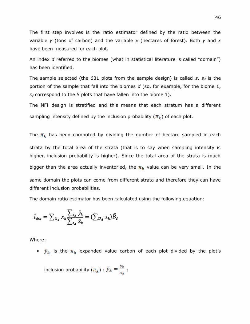
The first step involves is the ratio estimator defined by the ratio between the

variable y (tons of carbon) and the variable x (hectares of forest). Both y and x

have been measured for each plot.

An index d referred to the biomes (what in statistical literature is called “domain”)

has been identified.

The sample selected (the 631 plots from the sample design) is called s. sd is the

portion of the sample that fall into the biomes d (so, for example, for the biome 1,

sd correspond to the 5 plots that have fallen into the biome 1).

The NFI design is stratified and this means that each stratum has a different

sampling intensity defined by the inclusion probability ( ) of each plot.

The has been computed by dividing the number of hectare sampled in each

strata by the total area of the strata (that is to say when sampling intensity is

higher, inclusion probability is higher). Since the total area of the strata is much

bigger than the area actually inventoried, the value can be very small. In the

same domain the plots can come from different strata and therefore they can have

different inclusion probabilities.

The domain ratio estimator has been calculated using the following equation:

Where:

is the expanded value carbon of each plot divided by the plot’s

inclusion probability ( ) : ;

47

is the expanded value of hectares of forest of each plot divided by the

plot’s inclusion probability ( ): .

The domain ratio estimator provides the total domain. The average has been

calculated dividing by the size of the domain as follow:

This calculation has been used to compute the estimates per hectare for each

Biome.

The variance computation proposed by the Sarndal methodology is:

where:

is the -expanded value of the residuals eks divided by the inclusion

probability:

and:

and the -expanded covariance of sampling indicators and variance

indicated by the Bernouilli pairwise plot selection probabilities:

where each pair of plots are here indexed using k and l.

48

When the plots k and l come from different strata, their selection has been

independent:

and is therefore 0.

When the plots k and l come from the same stratum then:

While

As k and l are from the same plot and from the same stratum .

is then computed as:

For N very big (as it is in our case) approximates to 0.

For k=l, approximates to 1

To summarize, the

49

equals 0 whenever k is different from l.

The variance formula can be then approximated to:

where B is a biome-specific factor akin to a slope in a regression between y and x.

The comparative advantage with this approach is that the result is not

approximated or inaccurate conversely as the Biomes and Strata does not overlap

the variance values are higher in the new estimates because composed by the

Strata variance and the Biome variance.

In order to correctly apply the BGB ratios from IPCC(2006), the ecological zone

layers have been applied.

The result is a not homogeneous distribution of the plot in the biomes:

Table 16: distribution of the plots per Biome and Ecological Zones:

Ecological Zones

Biomes

Tropicaldesert

Tropicaldry for-

est

Tropicalmoist de-ciduousforest

Tropicalmoun-

tainsystem

Tropicalshrub-land

WaterTotal

Result

Acacia-Commiphora 18 54 123 195Combretum-Terminalia 43 13 92 31 179Dry Afromontaine 1 148 2 151Moist Afromontaine 1 7 85 93Others 1 1 2 4 1 9

Total 19 46 20 381 160 1 627

This is the reason for the not direct correspondence between AGB and BGB in all

the estimates.

The deadwood estimates have elevate uncertainty, this is a weel known problem

dued to many practical problems in measuring in the field and associated

uncertainties (IPCC, 2006)

50

Comparison of the NFI Results and Secondary Data Sources

Numerous studies have been undertaken in Ethiopia already assessing forest

carbon stock. To validate the results from the NFI the findings have been compared

against these secondary data sources. This secondary data and information was

obtained from various sources, some processed and other raw data, including MSc

theses, PhD dissertations, research reports, project reports and grey literature. For

some of the secondary sources, original data (raw data) were obtained from the

respective researchers and re-analysed. In total, 1602 sampling units were

involved, excluding the sample number from the WBISPP, 2004. The results of the

analysis of secondary data sources are given in Figure 12.

Most remarkable in the comparison of primary and secondary data is the strong

reduction of the confidence intervals of the NFI analysis compared to the secondary

data analysis and the large difference in AGB estimates for Dry and Moist

Afromontane forest, where the secondary sources suggest a much higher carbon

Figure 12: The average AGB (tC/ha) with their confidence intervals for forest in the 4

biomes is compared between primary (NFI) and secondary (literature and local studies)

data

51

contents (220% and 62% higher for Dry and Moist Afromontane forest

respectively). This difference is believed to be due to the sample design in the

secondary data which most likely targeted primary and dense forest patches.

Therefore, the NFI data is thought to be more representative for estimating

emissions and removals from country-wide forest area changes.

A further comparison has been done with the IPCC default values, showing a

substantial concordance with the NFI estimates (table 13 and figure 14).

9.2. RESULTS AND PROPOSED EMISSION FACTORS

The results of the analysis of the average forest carbon stock in the above ground

biomass (AGB), below ground biomass (BGB) and deadwood carbon pools are

provided in Figure 14, 15, 16 and table17 respectively. Ethiopia assumes total

oxidation of AGB, BGB and deadwood after forest conversion, therefore emission

factors are approximated by the full carbon stock in AGB, BGB and deadwood for

forest in the different biomes. The removal factor for forest gain is estimated as the

inverse of the emission factor therefore assuming full average carbon stock for each

hectare of gain detected. As such, in absence of specific values for the country,

Ethiopia does not take into account the age structure in the forest which would

Ecological zones

260 (160-430)

Tropical dry forest 120 (120-130)

Tropical shrubland* 70 (20-200)

Tropical mountain systems* 40-190

Above-ground biomass (t ha-1)

Tropical moist deciduous forest

Figure 13: IPCC 2006 default values. The asterisk

identifies the most represented ecological zones in

Ethiopia

52

introduce too much uncertainty (for the time being). Assuming the full carbon stock

is removed from the atmosphere at the time gain is detected may over-estimate

the removals corresponding to the early years of forest growth. However, this may

be compensated by the fact that gain is generally detected by remote sensing in a

later stage of growth (therefore removals already preceded the time of detection).

Figure 14: Above ground biomass per biome

53

Figure 15: Below ground biomass per biome

Figure 16: Deadwood per biome

54

Above Ground Biomass

Biomes c.i. (95%)

Acacia-Commiphora 39.99 47.71Combretum-Terminalia 61.66 26.20Dry Afromontane 115.32 64.61Moist Afromontane 197.83 49.77

Below Ground Biomass

Biomes c.i. (95%)

Acacia-Commiphora 19.67 27.74Combretum-Terminalia 18.72 7.53Dry Afromontane 31.14 18.35Moist Afromontane 53.62 21.96

Deadwood

Biomes c.i. (95%)

Acacia-Commiphora 0.37 0.83Combretum-Terminalia 1.31 0.78Dry Afromontane 2.58 3.79Moist Afromontane 2.26 0.95

AGB (t ha-1)

BGB (t ha-1)

Total Carbon (t ha-1)

Table 17: AGB, BGB and DW per hectare per biome

55

10. RELEVANT POLICIES, PLANS AND FUTURE CHANGES

Ethiopia’s development agenda is governed by two key strategies: the Second

Growth and Transformation Plan (GTP-2) and the Climate Resilient Green Economy

(CRGE) strategy. Both strategies prioritize attainment of middle income status by

2025 and, through the CRGE Strategy, to achieve this by taking low carbon,

resilient, green growth actions. Both strategies emphasize agriculture and forestry,

The CRGE Strategy targets 7 million hectares for forest expansion. GTP-2 Goal 15

aims to: “Protect, restore and promote sustainable use of terrestrial ecosystems by

managing forests, combating desertification, and halting and reversing land

degradation and halt biodiversity loss.”

The strategic directions of the forest sector in GTP-2 are enabling the community to

actively participate in environmental protection and forest development activities,

and implementing the green economy strategy at all administration levels and

embarking on environmental protection and forest development at a scale. In the

GTP-2, the sector has thus set goals mainly in relation to building climate resilient

green economy, environmental protection and forest development. This will be

applied mainly in priority sectors identified by the CRGE strategy. In addition,

mobilizing resources which can enable to fully implement the CRGE strategy is also

another goal of the sector. In terms of forest development, the aim is to increase

the share of the forest sector in the overall economy. The strategy also aims to

increase the forest coverage through research-based forest development. A target

set during the GTP-2, is to reduce deforestation by half .

56

11. PROPOSED FOREST REFERENCE LEVEL

11.1. CONSTRUCTION APPROACH AND PROPOSED FORESTREFERENCE EMISSION LEVEL FOR DEFORESTATION AND FORESTREFERENCE LEVEL FOR AFFORESTATION

Ethiopia proposes a Forest Reference Emission Level based on average annual

emissions and removals over the period 2000-2013 assessed by AD x EF. The

emissions from deforestation in the FRL are assessed at 17.7 mln t CO2 e/yr while

the removals from afforestation are assessed at 4.9 mln t CO2 e/yr.

Figure 17: Emission per biome per year.

57

Figure 18: Removals per biome per year

58

12. UPDATING FREQUENCY

In order to ensure the accuracy of the FRL with updated socio-economic conditions

and in order to incorporate new or improved data that may be available, the FRL

will be revised periodically. Ethiopia proposed this FRL to be valid at least 5 years,

yet it may be improved or completed more frequently. Ethiopia is also evaluating

the possibility to undergone a new forest inventory, region based with a 5 years

cycle.

59

13. FUTURE IMPROVEMENTS

Forest degradation is believed to be an important source of emissions by Ethiopia

and several measures are being put in place to reduce emissions from forest

degradation (e.g. the promotion of energy efficient cooking stoves, planting trees

on-farm boundaries for fuelwood and the provision of non-wood and alternative

energy sources). Therefore, Ethiopia is strongly interested in testing and

developing a cost-effective, robust and reliable method for consistent measuring

and monitoring of emissions from forest degradation for its future inclusion in the

FRL.

60

14. REFERENCES

1. Breiman, L., Freidman, JH, Olshen, RA, and Stonem CJ. 1984. Classificationand regression trees. Wadsworth, Belmont CA.

2. Breiman. 2001. Random Forests. Machine Learning. 45, 2-32.https://www.stat.berkeley.edu/~breiman/RandomForests/cc_home.htm

3. CGIAR-CSI SRTM 90m DEM Digital Elevation Database, versión 4. CGIARConsortium for Spatial Information (CGIAR-CSI). URL:http://srtm.csi.cgiar.org/Index.asp

4. Bodart, C., Brink A., Donnay F., Lupi, A., Mayaux, P., & Achard, F. (2013).Continental estimates of forest cover and forest cover changes in the dryecosystems of Africa between 1990 and 2000. Journal of biogeography,40(6), 1036-1047.

5. Brown, S. (1997). Estimating biomass and biomass change of tropicalforests: a Primer. FAO Forestry Paper 134:120-130.

6. Brown, S. (2002). Measuring carbon in forests: current status and futurechallenges. Environmental Pollution 116: 363-372.

7. Brown, S. and A. E. Lugo (1990). Tropical secondary forests. Journal ofTropical Ecology 6:1-32.

8. Brown, S. and Lugo, A. (1982). The storage and production of organic matterin tropical forests and their role in the global carbon cycle. Biotropica 14:161-187.

9. Brown, S.A.J., Gillespie, J.R. and Lugo, A.E.(1989). Biomass estimationmethods for tropical forests with application to forest inventory data. ForestScience 35: 110-115.

10. Chave J, Coomes D, Jansen S. 2009. Towards a worldwide woodeconomics spectrum. Ecology Letters, 12, 351–366.

11. Chave, J., Andalo, C., Brown, S., Cairns, M.A., Chambers, J.Q., Eamus,D., Fölster, H.,Fromard, F., Higuchi, N., Kira, T., Lescure, J.-P., Nelson, B.,Ogawa, H., Puig, H.,Riéra, B., Yamakura, T., 2005. Tree allometry andimproved estimation of carbon stocks and balance in tropical forests.Oecologia 145, 87–99.

12. Cornelissen, J. H. C., S. Lavorel, E. Garnier, S. Diaz, N. Buchmann, D.E. Gurvich, P. B. Reich, H. ter Steege, H. D. Morgan, M. G. A. van derHeijden, J. G. Pausas, and H. Poorter. 2003. A handbook of protocols forstandardized and December 2006 WOOD DENSITY IN NEOTROPICALFORESTS 2365 easy measurement of plant functional traits worldwide.Australian Journal of Botany 51:335–380.

13. CSA (2007). Population and Housing Census Report-Country – 2007(http://www.csa.gov.et/index.php/2013-02-20-14-51-51/2013-04-01-11-53-00/census-2007)

14. Demel Teketay, Mulugeta Lemenih, Tesfaye Bekele, Yonas Yemshaw,Sisay Feleke, Wubalem Tadesse, Yitebitu Moges, Tesfaye Hunde & DemekeNigussie (2010). Forest Resources and Challenges of Sustainable ForestManagement and Conservation in Ethiopia. In: Bongers F & T. Tennigkeit

61

(eds). Degraded forests in Eastern Africa: management and restoration.Earthscan Publications.

15. FAO & JRC. 2012. Global forest land-use change 1990–2005, by E.J.Lindquist, R. D’Annunzio, A. Gerrand, K. MacDicken, F. Achard, R. Beuchle, A.Brink, H.D. Eva, P. Mayaux, J. San-Miguel-Ayanz & H-J. Stibig. FAO ForestryPaper No. 169. Food and Agriculture Organization of the United Nations andEuropean Commission Joint Research Centre. Rome, FAO.http://www.fao.org/docrep/017/i3110e/i3110e.pdf

16. FAO 2015. Global forest Resources Assessment. Rome, Italy.17. FAO. 2015. Map Accuracy Assessment and Area Estimation: A Practical

Guide.18. Foody and Mathur. 2006. The use of small training sets containing

mixed pixels for accurate hard image classification: Training on mixedspectral responses for classification by a SVM. Remote Sensing ofEnvironment. 103:2, 179-189.

19. Friis, I., Demissew, S., & Breugel, P. V. (2010). Atlas of the potentialvegetation of Ethiopia. Det Kongelige Danske Videnskabernes Selskab.

20. FSR (2015). Ethiopia Forest Sector Review. Focus on commercialforestry and industrialization. UNIQUE forestry and land use / CONSCIENTIA,Addis Ababa, Ethiopia.

21. Hedberg, I. (1996). Flora of Ethiopia and Eritrea (pp. 802-804).Springer Netherlands.

22. GFOI. 2014. Space data services: Support for National ForestMonitoring Systems.http://www.gfoi.org/wp-content/uploads/2015/03/Space_Data_Services_External _v1.1.pdf

23. Hansen, M. C., et al. 2013. High-resolution global maps of 21st-century forest cover change. Science, 342(6160), 850-853.

24. Hijmans, R. J., Cameron, S. E., Parra, J. L., Jones, P. G., & Jarvis, A.2005. Very high resolution interpolated climate surfaces for global land areas.International Journal of Climatology 25: 1965-1978.

25. Hurni K, Zeleke G, Kassie M, Tegegne B, Kassawmar T, Teferi E, MogesA, Tadesse D, Ahmed M, Degu Y, Kebebew Z, Hodel E, Amdihun A, MekuriawA, Debele B, Deichert G, Hurni H. 2015. Economics of Land Degradation(ELD) Ethiopia Case Study. Soil Degradation and Sustainable LandManagement in the Rainfed Agricultural Areas of Ethiopia: An Assessment ofthe Economic Implications. Report for the Economics of Land DegradationInitiative. 94 pp.

26. Lehner, B. & Döll, P. (2004). Development and validation of a globaldatabase of lakes, reservoirs and wetlands. Journal of Hydrology 296: 1-22.

27. Helina Tilahun and Emily Schmidt (2012). Spatial Analysis of LivestockProduction Patterns in Ethiopia. ESSP II Working Paper 44, IFPRI, AddisAbaba, Ethiopia.

28. Mikrewongel Tadesse, A. B. (2015). Estimation of Carbon Stored inAgroforestry Practices in Gununo Watershed, Wolayitta Zone, Ethiopia.Journal of Ecosystem & Ecography, 05(01), 1–5.http://doi.org/10.4172/2157-7625.1000157

29. Olofsson, P., Foody, G. M., Stehman, S. V., & Woodcock, C. E. 2013.Making better use of accuracy data in land change studies: Estimating

62

accuracy and area and quantifying uncertainty using stratifiedestimation.Remote Sensing of Environment, 129, 122-131.

30. Olofsson, P., Foody, G. M., Herold, M., Stehman, S. V., Woodcock, C. E.,& Wulder, M. A. 2014. Good practices for estimating area and assessingaccuracy of land change. Remote Sensing of Environment, 148, 42-57.

31. Pearcy R. W., Ehleringer J. R., Mooney H. A., Rundel P. W. . 1989. Plantphysiological ecology. Chapman and Hall, New York, New York, USA.

32. Reusing, M. (2000). Change detection of natural high forests inEthiopia using remote sensing and GIS techniques. International Archives ofPhotogrammetry and Remote Sensing. Vol. XXXIII, Part B7. Amsterdam 2000

33. Reyes, G., S. Brown, J. Chapman, and A. E. Lugo. 1992. Wooddensities of tropical tree species. General Technical Report SO-88. USDAForest Service, Southern Forest Experiment Station, New Orleans, Louisiana,USA

34. Sarndal, B. Swensson, J. Wretman: Model Assisted Survey Sampling,Springer, New York, 1992

35. Simegn, T. Y., Soromessa, T., & Bayable, E. (2014). Forest CarbonStocks in Lowland Area of Simien Mountains National Park : Implication forClimate Change Mitigation, 7522(3), 29–36.

36. Tewkesbury, A. P., Comber, A. J., Tate, N. J., Lamb, A., & Fisher, P. F.2015. A critical synthesis of remotely sensed optical image change detectiontechniques. Remote Sensing of Environment, 160, 1-14.

37. De Vries P.G., 1986. Sampling theory for forest inventory. A teach-yourself course, Springer-Verlag, Berlin, 420 p.

38. WBISPP (2004). A strategic plan for the sustainable development,conservation and management of the woody biomass resources: Final report.Federal Democratic Republic of Ethiopia, Ministry of Agriculture. 60 pp.

39. Westerman R. L. 1990. Soil testing and plant analysis, 3rd ed. SoilScience Society of America, Madison, Wisconsin, USA.

40. de Wit, M. & Stankiewicz, J. 2006. Changes in Surface Water Supplyacross Africa with Predicted Climate Change. Science 311: 1917-1921.

41. Wolde, B. M., Kelbessa, E., & Soromessa, T. (2014). Original ResearchForest Carbon Stocks in Woody Plants of Arba Minch Ground Water Forest,7522(June), 141–147.

63

ANNEX

ANNEX I

Strata SUSU area

(Ha)Strata Area (Ha) Sampling Intensity

Samples

distribution (%)

Stratum I 107 214 4,058,626 5.27272E-05 59.0

Stratum II 135 270 39,339,300 6.86337E-06 7.7

Stratum III 137 274 19,689,121 1.39163E-05 15.6

Stratum IV 232 464 35,588,651 1.30379E-05 14.6

Stratum V 20 40 14,445,525 2.76902E-06 3.1

TOTALS 631 1,262 113,121,223 8.93138E-05 100

Biome SUSU area

(Ha)Biome Area (Ha) Sampling Intensity

Samples

distribution (%)

Acacia-Commiphora 195 390 58,654,959 6.64905E-06 9.7

Combretum-Terminalia 179 358 25,715,132 1.39218E-05 20.4

Dry Afromontaine 151 302 19,720,064 1.53144E-05 22.4

Moist Afromontaine 93 186 8,440,625 2.20363E-05 32.3

Others 9 18 1,736,549 1.03654E-05 15.2

TOTALS 627 1,254 114,267,329 6.82868E-05 100

Table 18: sampling distribution and sampling intensity comparisons between NFI strata and biomes.

NOTE:The difference between the number of SU (631 and 627) is due to the fact that 4 SU during the sampling design are

accidentally fall outside the national boundaries currently adopted.

64

ANNEX II

Table 19: Basic Wood Density of Indigenous and Exotic Tree Species in Ethiopia

No Scientific nameBasic Density(g/cm3) Reference

Dataquality* Remark

1 Acacia abyssinica 0.826 average of genus (ICRAF database) M

2 Acacia albida 0.562http://www.worldagroforestry.org/regions/southeast_asia/resources/db/wd M

3 Acacia asak 0.769 average of genus (ICRAF database) M 4 Acacia brevispica 0.769 >> M 5 Acacia bussei 0.769 >> M

6Acacia decurrens

0.816 Getachew Desalegn et al., 2012 HAir drydensity

7 Acacia dolichocephala 0.769 average of genus M 8 Acacia drepanolobium 0.769 >> M 9 Acacia etbaica 0.590 Vreugdenhil et al., 2012 H

10 Acacia gerrardii 0.775Tropical Africa: global database (Zanne et al.,2009) M

11 Acacia goetzei 0.883 >> M 12 Acacia hokii 0.769 average of genus (ICRAF database) M 13 Acacia Iahai 0.769 >> M 14 Acacia macrothyrsa 0.769 >> M 15 Acacia mellifera 0.482 Vreugdenhil et al., 2012 H 16 Acacia mollis 0.482 Vreugdenhil et al., 2012 H 17 Acacia nilotica 0.723 Vreugdenhil et al., 2012 H 18 Acacia oerofota 0.769 average of genus M 19 Acacia pentagon 0.826 average of genus (ICRAF database) M 20 Acacia polyacantha 0.769 average of genus M 21 Acacia reficiens 0.769 >> M 22 Acacia robusta 0.769 >> M 23 Acacia senegal 0.741 Vreugdenhil et al., 2012 H 24 Acacia seyal 0.497 Vreugdenhil et al., 2012 H 25 Acacia sieberiana 0.769 average of genus M 26 Acacia tortilis 0.590 Vreugdenhil et al., 2012 H 27 Acacia xiphocarpa 0.769 average of genus M 28 Acacia Zanzibarica 0.769 average of genus M 29 Acallypha acrogyna 0.300 A. Cauturus (Zanne et al.; global database), L 30 Acanthus sp. 0.592 Global database (Zanne et al., 2009) M

31Acokantheraschimperi 0.784

Acokanthera oppositifolia (from Globaldatabase) L

32Acrocarpusfraxinifolius 0.610 Getachew Desalegn et al., 2012 H

air drydensity

33 Adansonia digitata 0.590 Vreugdenhil et al., 2012 H

34Adathadaschimperiana 0.640

same species from wood density for trees ofUganda L

35 Alangium chinense 0.420http://db.worldagroforestry.org//wd/species/Alangium_chinense M

36 Alangium Chinese 0.408 >> M 37 Albizia aylemeri 0.579 Genus average M

38 Albizia glaberiima 0.555http://db.worldagroforestry.org//wd/species/Alangium_chinense M

39 Albizia 0.534 Albizia gummifera L

65

No Scientific nameBasic Density(g/cm3) Reference

Dataquality* Remark

grandibracteata

40Albizia gummifera

0.580 Getachew Desalegn et al., 2012 Hair drydensity

41 Albizia lebbeck 0.596http://db.worldagroforestry.org//wd/species/Alangium_chinense M

42 Albizia lophantha 0.579 Genus average M 43 Albizia malacophylla 0.579 Genus average M

44 Albizia schimperiana 0.530 Getachew Desalegn et al., 2012 Hair drydensity

45 Alchernea laxiflora 0.525 A. hirtella; Zanne et al.; global database L

46Alchorneaeuphorbiacae 0.525 >> L

47Alihorneaeuphorbiscara 0.525 >> L

48Allophylusabyssinicus 0.580 Getachew Desalegn et al., 2012 H

air drydensity

49Allophylusabyssinicus 0.491 Vreugdenhil et al., 2012 H

50 Allophylus rubifolius 0.494 Genus average M

51 Alstonia boonei 0.387http://db.worldagroforestry.org//wd/species/Alstonia_boonei L

52 Annona crassiflora 0.400http://db.worldagroforestry.org//wd/species/Alstonia_boonei L

53 Anogeissus leiocarpa 0.880 >> L 54 Antialis toxicalia 0.432 Antiaris africana; L

55 Antiaris toxicaria 0.470 Getachew Desalegn et al., 2012 Hair drydensity

56 Apodytes dimidiata 0.610http://db.worldagroforestry.org//wd/genus/Apodytes M

57 Apodytes dimidiata 0.710 Getachew Desalegn et al., 2012 Hair drydensity

58Argomaelleramaerophylla 0.640 Wood density of trees of Uganda L

59 Arundinaria alpine 0.630 Getachew Desalegn et al., 2067 Hair drydesnity

60 Azadirachta indica 0.728http://db.worldagroforestry.org//wd/genus/Apodytes M

61 Balanites aegyptiaca 0.542 Vreugdenhil et al., 2012 H 62 Balanites glabra 0.684 Genus average M 63 Baphia abyssinica 0.559 B. Nitida (global database: Zanne et al., 2009) L 64 Berberis holstii 0.641 Genus average M

65 Berchemia discolor 0.895http://db.worldagroforestry.org//wd/genus/Apodytes M

66 Bersama abyssinica 0.671http://db.worldagroforestry.org//wd/genus/Bersama & also global database H

67 Blighia unijugata 0.700 Getachew Desalegn et al., 2012 Hair drydensity

68 Blighia unijugata 0.564http://db.worldagroforestry.org//wd/genus/Apodytes M

69Boswelliahildebrandtii 0.500 Boswellia sp L

70Boswelliamicrophylla 0.500 >> L

66

No Scientific nameBasic Density(g/cm3) Reference

Dataquality* Remark

71 Boswellia neglecta 0.500 >> L 72 Boswellia papyrifera 0.500 >> L 73 Boswellia rivae 0.500 >> L 74 Boswellia sp 0.500 Boswellia serrata (FAO data) L 75 Bridelia cathartica 0.587 Genus average M

76 Bridelia micrantha 0.540http://db.worldagroforestry.org//wd/genus/Apodytes M

77Bruceaantidysenterica 0.640 Wood density of Trees of Uganda L

78 Buddleia polystachya 0.400 Vreugdenhil et al., 2012 H 79 Caesalpinia trothae 0.951 Genus average M

80 Caesalpinia volkensii 0.951http://db.worldagroforestry.org//wd/genus/Caesalpinia) Genus average M

81 Callistemon citrinus 0.951 >> M 82 Calotropis procera 0.794 Genus average M 83 Canthium euryoides 0.643 Genus average M 84 Canthium giordanii 0.643 Genus average M

85Canthiumoligocarpum 0.643 Genus average M

86 Canthium setiglarum 0.643 Genus average M 87 Capparis cartilagenia 0.691 Genus average M 88 Capparis micrantha 0.691 Genus average M 89 Capsicum conicum 0.482 Vreugdenhil et al., 2012 H

90 Carissa edulis 0.650

Carissa spinariumhttp://www.hindawi.com/journals/tswj/2012/790219/tab1/ L

91 Cassia didymobotrya 0.745http://db.worldagroforestry.org//wd/genus/Apodytes M

92 Cassia sinqueana 0.706http://db.worldagroforestry.org//wd/genus/Apodytes M

93Cassipoureamalosana 0.673 Genus average M

94Casuarinaequisetifolia 0.766

http://db.worldagroforestry.org//wd/genus/Apodytes M

95 Catha edulis 0.658http://db.worldagroforestry.org//wd/genus/Apodytes M

96 Celtis africana 0.745http://db.worldagroforestry.org//wd/species/Celtis_africana M

97 Celtis africana 0.760 Getachew Desalegn et al., 2012 Hair drydensity

98 Celtis kranssiana 0.604 Genus average M 99 Celtis philippinensis 0.611 http://db.worldagroforestry.org//wd M 100 Celtis zenkeri 0.59 FAO database M

101Chaionanthusmildbraedii 0.705 Average Chionanthus L

102 Citrus aurantifolia 0.699 Genus average M 103 Citrus aurantium 0.699 Genus average M 104 Citrus grandis 0.590 http://db.worldagroforestry.org//wd M 105 Citrus medica 0.770 http://db.worldagroforestry.org//wd M 106 Citrus meolica 0.699 Genus average M 107 Citrus reticulata 0.699 Genus average M 108 Citrus sinensis 0.699 Genus average M

67

No Scientific nameBasic Density(g/cm3) Reference

Dataquality* Remark

109 Clausena anisata 0.482http://db.worldagroforestry.org//wd/species/Clausena_anisata M

110 Clematis hirsuta 0.526 Genus average M

111 Coffea arabica 0.620http://db.worldagroforestry.org//wd/species/Coffea_arabica M

112Combretumaculeatum 0.474 Vreugdenhil et al., 2012 H

113Combretumbinderianum 0.880 http://db.worldagroforestry.org//wd/species M

114 Combretum colinum 0.590 Vreugdenhil et al., 2012 H

115Combretumghasalense 0.845 http://db.worldagroforestry.org//wd/species M

116 Combretum molle 0.482 Vreugdenhil et al., 2012 H 117 Combretum voldensii 0.845 http://db.worldagroforestry.org//wd/species M 118 Commiphora africana 0.276 http://db.worldagroforestry.org//wd/species M 119 Commiphora africana 0.482 Vreugdenhil et al., 2012 H

120Commiphoraalaticaulis 0.389 http://db.worldagroforestry.org//wd/species M

121 Commiphora billia 0.389 http://db.worldagroforestry.org//wd/species M

122Commiphorabioviniana 0.646 http://db.worldagroforestry.org//wd/species M

123Commiphoraboranensis 0.389 Genus average M

124 Commiphora bruceau 0.389 Genus average M 125 Commiphora confusa 0.389 Genus average M

126Commiphoraellenbeckii 0.389 Genus average M

127Commiphoraerlangeriana 0.389 Genus average M

128Commiphoraerythraea 0.389 Genus average M

129Commiphorahabessinica 0.389 Genus average M

130Commiphoraogadensis 0.389 Genus average M

131Commiphoraschimperi 0.389 Genus average M

132Commiphorasphaerophylla 0.389 Genus average M

133 Commiphora tenuis 0.389 Genus average M

134 Cordia africana 0.482http://db.worldagroforestry.org//wd/species/Cordia_africana M

135 Cordia africana 0.410 Getachew Desalegn et al., 2012 Hair drydensity

136 Cordia allliodora 0.390 Getachew Desalegn et al., 2012 Hair drydensity

137 Cordia monoica 0.482 Vreugdenhil et al., 2012 H 138 Cordia ovalis 0.544 Genus average M

139Crasocephalummontuosum 0.331 C. Manii M

140Crassocephalusmontus 0.331 C. Manii M

141 Croton dichogamus 0.525 Genus average M

68

No Scientific nameBasic Density(g/cm3) Reference

Dataquality* Remark

142Crotonmacrostachyus 0.518

http://db.worldagroforestry.org//wd/species/Croton_macrostachyus M

143Crotonmacrostachyus 0.560 Getachew Desalegn et al., 2012 H

air drydensity

144 Cupressus lusitanica 0.430 Getachew Desalegn et al., 2012 Hair drydensity

145 Cussonia holstii 0.409 Genus average M 146 Cussonia ostinii 0.409 Genus average M 147 Dalbergia boehmii 0.821 Genus average M

148Dalbergiamelanoxylon 0.728 Vreugdenhil et al., 2012 H

149 Dichrostachys cinerea 0.482 Vreugdenhil et al., 2012 H

150 Diospyros abyssinica 0.790 Getachew Desalegn et al., 2012 Hair drydensity

151Diospyrosmespiliformis 0.758 Genus average M

152Discopodiumpenninervium 0.482 Vreugdenhil et al., 2012 H

153Dodonaeaangustifolia 1.040 http://db.worldagroforestry.org//wd/species M

154 Dombeya bruceana 0.580 Genus average M 155 Dombeya quenguesta 0.580 Genus average M 156 Dombeya torrida 0.451 Vreugdenhil et al., 2012 H 157 Dombeya torrida 0.588 http://db.worldagroforestry.org//wd/species M 158 Dovyalis abyssinica 0.579 http://db.worldagroforestry.org//wd/species M

159Dracaenaafromontane 0.418 Genus average M

160 Dracaena fragrans 0.418

genus average(http://db.worldagroforestry.org//wd/genus/Dracaena) M

161 Dracaena steudneri 0.418 >> M 162 Ehretia cymosa 0.560 http://globalspecies.org/ntaxa/2529407 L 163 Ehretia cymosa 0.484 http://db.worldagroforestry.org//wd/species M

164 Ekebergia capensis 0.580 Getachew Desalegn et al., 2012 Hair drydensity

165 Embelia schimperi 0.775 Embelia oleifera L 166 Erica arborea 0.357 Vreugdenhil et al., 2012 H

167 Erythrina abyssinica 0.426http://db.worldagroforestry.org//wd/species/Erythrina_abyssinica M

168 Erythrina brucei 0.314

Genus averagehttp://db.worldagroforestry.org//wd/genus/Erythrina M

169Erythrococcaabyssinica 0.58 Average of tropical Africa L

170 Erythrococca Kirkii 0.58 Average of tropical Africa L

171Erythrococcatrichogynol 0.58 Average of tropical Africa L

172Erythroxylumfisherriii 0.802

Average Genus(http://db.worldagroforestry.org//wd/genus/Erythroxylum) M

173Eucalyptuscamaldulensis 0.853 Getachew Desalegn et al., 2012 H

air drydensity

174 Eucalyptus citriodora 0.830 http://db.worldagroforestry.org//wd/species M

69

No Scientific nameBasic Density(g/cm3) Reference

Dataquality* Remark

175 Eucalyptus deanei 0.570 Getachew Desalegn et al., 2012 Hair drydensity

176 Eucalyptus deglupta 0.410 Getachew Desalegn et al., 2012 Hair drydensity

177Eucalyptusdelegatensis 0.530 Getachew Desalegn et al., 2012 H

air drydensity

178 Eucalyptus dunii 0.610 Getachew Desalegn et al., 2012 Hair drydensity

179 Eucalyptus fastigata 0.650 Getachew Desalegn et al., 2012 Hair drydensity

180 Eucalyptus globulus 0.780 Getachew Desalegn et al., 2012 Hair drydensity

181 Eucalyptus grandis 0.560 Getachew Desalegn et al., 2012 Hair drydensity

182 Eucalyptus grandis 0.665 http://db.worldagroforestry.org//wd/species M

183Eucalyptusmicrocorys 0.860 Getachew Desalegn et al., 2012 H

air drydensity

184 Eucalyptus nitens 0.760 Getachew Desalegn et al., 2012 Hair drydensity

185 Eucalyptus obliqua 0.670 Getachew Desalegn et al., 2012 Hair drydensity

186 Eucalyptus paniculata 0.830 Getachew Desalegn et al., 2012 Hair drydensity

187 Eucalyptus pilularis 0.948 Getachew Desalegn et al., 2012 Hair drydensity

188 Eucalyptus regnans 0.480 Getachew Desalegn et al., 2012 Hair drydensity

189 Eucalyptus saligna 0.680 Getachew Desalegn et al., 2012 Hair drydensity

190 Eucalyptus viminalis 0.670 Getachew Desalegn et al., 2012 Hair drydensity

191 Euclea schimperi 0.741http://db.worldagroforestry.org//wd/species/Erythrina_abyssinica M

192 Euphorbia abyssinica 0.471 http://db.worldagroforestry.org//wd/species M

193Euphorbiacandelabrum 0.471 genus average M

194 Euphorbia sp. 0.314 Vreugdenhil et al., 2012 H 195 Euphorbia tirucallii 0.471 genus average M

196Fagaropsisangolensis 0.700 Getachew Desalegn et al., 2012 H

air drydensity

197 Faurea saligna 0.704 http://db.worldagroforestry.org//wd/species M 198 Ficus brachypoda 0.441 http://db.worldagroforestry.org//wd/species M 199 Ficus elastica 0.607 http://db.worldagroforestry.org//wd/species M 200 Ficus exasperata 0.377 http://db.worldagroforestry.org//wd/species M 201 Ficus gnaphalocarpa 0.441 Genus average M

202 Ficus mucuso 0.441

Average Ficus(http://db.worldagroforestry.org//wd/genus/Ficus) M

203 Ficus oxata 0.441 >> M 204 Ficus sp. 0.482 Vreugdenhil et al., 2012 H 205 Ficus sur 0.441 http://globalspecies.org/ntaxa/869708 L 206 Ficus sycomorus 0.422 http://globalspecies.org/ntaxa/869708 L 207 Ficus sycomorus 0.482 Vreugdenhil et al., 2012 H

70

No Scientific nameBasic Density(g/cm3) Reference

Dataquality* Remark

208 Ficus thonningii 0.432 http://globalspecies.org/ntaxa/911819 M

209 Ficus vasta 0.441

Average Ficus(http://db.worldagroforestry.org//wd/genus/Ficus) M

210 Filicium decipiens 0.960 http://db.worldagroforestry.org//wd/species M 211 Flacourtia indica 0.778 http://db.worldagroforestry.org//wd/species M 212 Flueggea virosa 0.770 Genus average M 213 Foeniculum vulgare 0.58 Average of tropical Africa L 214 Galiniera saxifraga 0.399 Vreugdenhil et al., 2012 H 215 Gardenia ternifolia 0.672 Genus average M 216 Gardenia volkensii 0.571 Vreugdenhil et al., 2012 H

217 Grevillea robusta 0.530 Getachew Desalegn et al., 2012 Hair drydensity

218 Grewia auriculifera 0.583 http://db.worldagroforestry.org//wd/species M 219 Grewia bicolor 0.456 Vreugdenhil et al., 2012 H 220 Grewia ferruginea 0.583 Genus average M 221 Grewia flavescens 0.583 Genus average M 222 Grewia mollis 0.583 Genus average M 223 Grewia tembensis 0.583 Genus average M 224 Grewia tenax 0.583 Genus average M 225 Grewia trichocarpa 0.583 Genus average M 226 Grewia villosa 0.482 Vreugdenhil et al., 2012 H

227 Hagenia abyssinica 0.591http://db.worldagroforestry.org//wd/species/Hagenia_abyssinica M

228 Hagenia abyssinica 0.560 Getachew Desalegn et al., 2012 Hair drydensity]

229 Halleria lucida 0.715 http://db.worldagroforestry.org//wd/species M

230Haplocoelumfoliolosum 0.788 http://db.worldagroforestry.org//wd/species M

231Heteromorphatrifoliata 0.58 Average of tropical Africa L

232 Hildebrandtia africana 0.58 Average of tropical Africa L 233 Hippocratae africana 0.876 H. maingayi L

234Hippocrateamacrophylla 0.876 H. maingayi L

235 Hippocratea pallens 0.876 H. maingayi L

236 Hypericum revolutum 0.726 Genus average M 237 Ilex mitis 0.466 Vreugdenhil et al., 2012 H 238 Indigofera garekeana 0.580 Average of tropical Africa L

239Jasminumabyssinicum 0.580 Average of tropical Africa L

240 Juniperus procera 0.628http://db.worldagroforestry.org//wd/genus/Juniperus M

241 Juniperus procera 0.540 Getachew Desalegn et al., 2012 Hair drydensity]

242 Justicia schimperiana 0.580 Average of tropical Africa L 243 Kigelia eethopun 0.661 http://db.worldagroforestry.org//wd/genus M 244 Kirkia burgeri 0.661 >> M 245 Lannea fruticosa 0.515 http://db.worldagroforestry.org//wd/genus M 246 Lannea schimperi 0.515 Genus average M 247 Lannea stuhlmannii 0.515 >> M

71

No Scientific nameBasic Density(g/cm3) Reference

Dataquality* Remark

248 Lannea welwitschii 0.405http://db.worldagroforestry.org//wd/species/Lannea_welwitschii M

249 Lantana trifolia 0.58 Average of tropical Africa L

250Lecaniodiscusfraxinifolius 0.405 >> L

251Lecaniodiscuslaxiflorus 0.405 >> L

252Lepidotrichiliavolkensii 0.58 Average of tropical Africa L

253 Lippia citriodora 0.700 Lippia mcvaughii L 254 Lippia javanica 0.700 >> L 255 Lippia spp. 0.700 >> L

256Lonchocarpuslaxiflorus 0.761 genus average M

257 Lonicera johnstonii 0.58 Average of tropical Africa L 258 Lycium europaeum 0.58 Average of tropical Africa L 259 Macaranga capenesis 0.416 global data base M

260Macarangakilimandscharica 0.404

Genus average(http://db.worldagroforestry.org//wd/genus/Macaranga) M

261 Maerua angolensis 0.58 Average of tropical Africa L 262 Maerua calophylla 0.58 Average of tropical Africa L 263 Maerua crassifolia 0.58 Average of tropical Africa L

264 Maesa lanceolata 0.676Genus average(http://db.worldagroforestry.org//wd/genus M

265 Magnifera indica 0.630 Wood density of trees of Uganda L

266 Malacantha alnifolia 0.450http://db.worldagroforestry.org//wd/genus/Malacantha M

267 Manilkara butugi 0.880 Getachew Desalegn et al., 2012 Hair drydensity]

268 Manilkora butugi 0.953 Average Genus, Africa M

269 Maytenus addat 0.713

Genusaverage(http://db.worldagroforestry.org//wd/genus/Maytenus) M

270 Maytenus arbutifolia 0.713

Genusaverage(http://db.worldagroforestry.org//wd/genus/Maytenus) M

271 Maytenus auriculifera 0.713

Genusaverage(http://db.worldagroforestry.org//wd/genus/Maytenus) M

272 Maytenus gracilipes 0.713 Average Genus, Africa M

273Maytenusheterophylla 0.495 http://db.worldagroforestry.org//wd/genus M

274 Maytenus ovatus 0.403 Vreugdenhil et al., 2012 H

275Maytenussenegalensis 0.713 http://db.worldagroforestry.org//wd/genus M

276 Maytenus undatus 0.732 http://db.worldagroforestry.org//wd/genus M

277 Melacantha alnifolia 0.620 Average Genus, Africa M

278 Melia azedarach 0.463 http://db.worldagroforestry.org//wd/genus M

279Milicia excelsa 0.570

Getachew Desalegn et al., 2012 Hair drydensity]

280 Millettia ferruginea 0.738 Average Millettia, Africa M

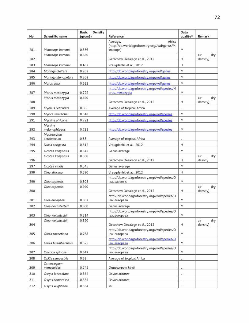
72

No Scientific nameBasic Density(g/cm3) Reference

Dataquality* Remark

281 Mimusops kummel 0.856

Average, Africa(http://db.worldagroforestry.org//wd/genus/Mimusops) M

282Mimusops kummel 0.880

Getachew Desalegn et al., 2012 Hair drydensity]

283 Mimusops kummel 0.482 Vreugdenhil et al., 2012 H

284 Moringa oleifera 0.262 http://db.worldagroforestry.org//wd/genus M

285 Moringa stenopetala 0.262 http://db.worldagroforestry.org//wd/genus M

286 Morus alba 0.622 http://db.worldagroforestry.org//wd/genus M

287 Morus mesozygia 0.722http://db.worldagroforestry.org//wd/species/Morus_mesozygia M

288Morus mesozygia 0.690

Getachew Desalegn et al., 2012 Hair drydensity]

289 Myenus reticulata 0.58 Average of tropical Africa L

290 Myrica salicifolia 0.618 http://db.worldagroforestry.org//wd/species M

291 Myrsine africana 0.721 http://db.worldagroforestry.org//wd/species M

292Myrsinemelanophloeos 0.732 http://db.worldagroforestry.org//wd/species M

293Mystroxylonaethiopicum 0.58 Average of tropical Africa L

294 Nuxia congesta 0.512 Vreugdenhil et al., 2012 H

295 Ocotea kenyensis 0.545 Genus average M

296Ocotea kenyensis 0.560

Getachew Desalegn et al., 2012 Hair drydesnity

297 Ocotea viridis 0.545 Genus average M

298 Olea africana 0.590 Vreugdenhil et al., 2012 H

299 Olea capensis 0.805http://db.worldagroforestry.org//wd/species/Olea_capensis M

300Olea capensis 0.990

Getachew Desalegn et al., 2012 Hair drydensity]

301 Olea europaea 0.807http://db.worldagroforestry.org//wd/species/Olea_europaea M

302 Olea hochstetteri 0.800 Genus average M

303 Olea welwitschii 0.814http://db.worldagroforestry.org//wd/species/Olea_europaea M

304Olea welwitschii 0.820

Getachew Desalegn et al., 2012 Hair drydensity]

305 Olinia rochetiana 0.768http://db.worldagroforestry.org//wd/species/Olea_europaea M

306 Olinia Usamberansis 0.825http://db.worldagroforestry.org//wd/species/Olea_europaea M

307 Oncoba spinosa 0.647http://db.worldagroforestry.org//wd/species/Olea_europaea M

308 Opilia campestris 0.58 Average of tropical Africa L

309Ormocarpummimosoides 0.742 Ormocarpum kirkii L

310 Osryia lanceolata 0.854 Osyris arborea L

311 Osyris compressa 0.854 Osyris arborea L

312 Osyris wightiana 0.854 >> L

73

No Scientific nameBasic Density(g/cm3) Reference

Dataquality* Remark

313 Otestegia steudneri 0.58 Average of tropical Africa L

314 Oxyanthus sp. 0.525 Genus value M

315 Oxyanthus speciosus 0.525http://db.worldagroforestry.org//wd/species/Oxyanthus_speciosus M

316Oxytenantheraabyssinica 0.608 Getachew Desalegn et al., 2012 H

air drydensity]

317 Ozoroa insignis 0.715 Ozoroa longipetiolata L

318 Ozoroa pulcherrima 0.715 >> L

319 Pappea capensis 0.883http://db.worldagroforestry.org//wd/species/Oxyanthus_speciosus M

320 Persea americana 0.561http://db.worldagroforestry.org//wd/species/Oxyanthus_speciosus M

321 Peterocarpus lucens 0.58 Average of tropical Africa L

322 Piliostigma thonningii 0.371 Vreugdenhil et al., 2012 H

323Pinus patula 0.450

Getachew Desalegn et al., 2012 Hair drydensity]

324Pinus radiata 0.450

Getachew Desalegn et al., 2012 Hair drydensity]

325 Pistacia falcata 0.720http://db.worldagroforestry.org//wd/species/Oxyanthus_speciosus M

326 Pistacia lentiscus 0.720 Genus average M

327Pittosporumabyssinicum 0.645

Genus average(http://db.worldagroforestry.org//wd/species/Pittosporum_abyssinicum) M

328Pittosporumviridiflorum 0.633

http://db.worldagroforestry.org//wd/species/Oxyanthus_speciosus M

air drydensity]

329 Podocarpus falcatus 0.523

Genus average(http://db.worldagroforestry.org//wd/genus/Podocarpus) M

330Podocarpus falcatus 0.520

Getachew Desalegn et al., 2012 Hair drydensity]

331 Polyscias ferruginea 0.286http://db.worldagroforestry.org//wd/species/Polyscias_ferruginea M

332Polyscias fulva

0.440 Getachew Desalegn et al., 2012 Hair drydensity]

333 Polyscious ferrogenia 0.38 Polyscias nodosa L

334Pouteria adolfi-friederici 0.600 Getachew Desalegn et al., 2012 H

air drydensity]

335 Pouteria abyssinica 0.711

Genus average(http://db.worldagroforestry.org//wd/species/Pouteria) M

336 Pouteria altissima 0.442http://db.worldagroforestry.org//wd/species/Pouteria_altissima M

337 Premna schimperi 0.658

Average Genus(http://db.worldagroforestry.org//wd/genus/Premna) M

338Prosopis juliflora

0.827 Getachew Desalegn et al., 2012 Hair drydensity]

339 Protea gaguedi 0.663 Protea angolensis L

340Prunus africana

0.850 Getachew Desalegn et al., 2012 Hair drydensity]

341 Prunus persica 0.588 Genus average M

74

No Scientific nameBasic Density(g/cm3) Reference

Dataquality* Remark

(http://db.worldagroforestry.org//wd/species/Pouteria)

342Pseudocedrelakotschyi 0.621

http://db.worldagroforestry.org//wd/species/Pouteria_altissima M

343 Psidium guajava 0.859

Genus average(http://db.worldagroforestry.org//wd/species/Pouteria) M

344 Psydrax schimperiana 0.743

Genus average(http://db.worldagroforestry.org//wd/species/Pouteria) M

345Pterolobiumstellatum 0.58 Average of tropical Africa L

346 Rabus steudneri 0.58 Average of tropical Africa L

347Rapaneamelanophixas 0.732

http://db.worldagroforestry.org//wd/species/Pouteria_altissima M

348 Rapanea simensis 0.722 genus average L

349 Rhamnus prinoides 0.579 genus average L

350 Rhamnus sp. 0.579 Genus average L

351 Rhinorea friisii 0.689 R. ferruginea L

352 Rhinorea laxiflora 0.689 R. ferruginea L

353 Rhoicissus tridentala 0.538 R. revoilii L

354 Rhus glutinosa 0.620 genus average M

355 Rhus natalensis 0.620 genus average M

356 Rhus retinorrhoea 0.620 genus average M

357 Rhus vulgaris 0.620 genus average M

358Rothmaniaurcelliformis 0.642 Africa (extratropical): global database L

359Rothmanniawhitfieldii 0.745 R. Fischeri: global database L

360 Rubus steudneri 0.350 Rubus alceifolius: global database L

361 Rumex nervousus 0.58 Average of tropical Africa M

362 Salix subserata 0.525http://db.worldagroforestry.org//wd/species/Sapium_ellipticum M

363 Sapium ellipticum 0.576http://db.worldagroforestry.org//wd/species/Sapium_ellipticum M

364 Schefflera abyssinica 0.405http://db.worldagroforestry.org//wd/species/Schefflera_abyssinica M

365 Schefflera abyssinica 0.491 Vreugdenhil et al., 2012 H

366 Schefflera volkensii 0.405http://db.worldagroforestry.org//wd/species/Schefflera_abyssinica M

367 Scherebera alata 0.790 Uganda data M

368 Sclerocarya birrea 0.515http://db.worldagroforestry.org//wd/species/Schefflera_abyssinica M

369Securidacalongepedunculata 0.880

http://db.worldagroforestry.org//wd/species/Schefflera_abyssinica M

370 Securindaca virosa 0.880 Securidaca longepedunculata L

371 Senna singueana 0.706http://db.worldagroforestry.org//wd/species/Schefflera_abyssinica M

372Sideroxylonoxyacantha 0.715

http://db.worldagroforestry.org//wd/species/Schefflera_abyssinica M

75

No Scientific nameBasic Density(g/cm3) Reference

Dataquality* Remark

373 Sideroxylon sp. 0.715http://db.worldagroforestry.org//wd/species/Schefflera_abyssinica M

374 Solanum incanum 0.428http://db.worldagroforestry.org//wd/species/Schefflera_abyssinica M

375 Spathodea nilotica 0.504http://db.worldagroforestry.org//wd/species/Schefflera_abyssinica M

376Steganotaeniaaraliacea 0.370 Uganda data M

377 Sterculia africana 0.482 Vreugdenhil et al., 2012 H

378 Sterculia setigera 0.320http://db.worldagroforestry.org//wd/species/Schefflera_abyssinica M

379Stereospermumkunthianum 0.741 Vreugdenhil et al., 2012 H

380 Strychnos innocua 0.870http://db.worldagroforestry.org//wd/species/Schefflera_abyssinica M

381 Strychnos mitis 0.733http://db.worldagroforestry.org//wd/genus/Strychnos M

382 Strychnos spinosa 0.733 genus average M

383 Syzygium guineense 0.712http://db.worldagroforestry.org//wd/genus/Syzygium M

384Syzygium guineense

0.740 Getachew Desalegn et al., 2012 Hair drydensity]

385 Tamarindus indica 0.624 Vreugdenhil et al., 2012 H

386 Tapura fisherii 0.660 Genus average: global database M

387 Teclea nobilis 0.798http://db.worldagroforestry.org//wd/genus/Teclea M

388 Teclea simplicifolia 0.798 Teclea nobilis L

389 Terminalia laxiflora 0.654 genus average M

390 Terminalia brownii 0.654

Average of genus(http://db.worldagroforestry.org//wd/genus/Terminalia) M

391 Terminalia brownii 0.495 Vreugdenhil et al., 2012 H

392 Terminalia laxiflora 0.574 Vreugdenhil et al., 2012 H

393Terminaliamacroptera 0.819

http://db.worldagroforestry.org//wd/genus/Teclea M

394 Terminalia mollis 0.654 genus average M

395Terminaliaprundioides 0.654 genus average M

396Terminaliaschimperiana 0.654 genus average M

397 Terminalia sopinos 0.654 genus average M

398 Thunbergia alata 0.640 Uganda data M

399 Toddalia asiatica 0.798 Toddalia nobilis L

400 Trema guineensis 0.366 genus average M

401 Trema orientalis 0.366 genus average M

402 Trichilea prieuriana 0.647http://db.worldagroforestry.org//wd/species/Trichilia_prieuriana M

403 Trichilia dregeana 0.482http://db.worldagroforestry.org//wd/species/Trichilia_prieuriana M

404 Trichilia 0.622 http://db.worldagroforestry.org//wd/species/T M

76

No Scientific nameBasic Density(g/cm3) Reference

Dataquality* Remark

madagascariense richilia

405 Trichilia pouerianu 0.622http://db.worldagroforestry.org//wd/species/Trichilia M

406Trichocladusellipticus 0.640 Uganda data M

407Trilepisiummadagariense 0.499

http://db.worldagroforestry.org//wd/species/Trilepisium_madagariense M

408Trilepisiummadagascariense 0.560 Getachew Desalegn et al., 2012 H

409Urerahypselodendron 0.324

average of genus(http://db.worldagroforestry.org//wd/genus/Urera) M

air drydensity

410 Vepris dainellii 0.700 Vepris undulate L

411 Vernonia amygdalina 0.413

average(http://db.worldagroforestry.org//wd/genus/Vernonia) M

412 Vernonia auriclifera 0.413

average(http://db.worldagroforestry.org//wd/genus/Vernonia) M

413Warburgiaugandensis 0.865

http://db.worldagroforestry.org//wd/species/Warburgia_ugandensis M

414Warburgiaugandensis 0.770 Getachew Desalegn et al., 2012 H

air drydensity]

415 Ximenia americana 0.867http://db.worldagroforestry.org//wd/species/Warburgia_ugandensis M

416 Ximenia caffra 0.812 genus average M

417Zanthoxylumchalybeum 0.629

http://db.worldagroforestry.org//wd/species/Warburgia_ugandensis M

418 Ziziphus mauritania 0.711http://db.worldagroforestry.org//wd/species/Warburgia_ugandensis M

419 Ziziphus mucronata 0.758http://db.worldagroforestry.org//wd/species/Warburgia_ugandensis M

420 Ziziphus spina-christi 0.482 Vreugdenhil et al., 2012 H * data quality refers to author’s personal judgement of the goodness of the woo density value depending on whether they are locallyrelevant or not. L = low; M = medium and H = high quality.