etd.pdf - NCSU Repository

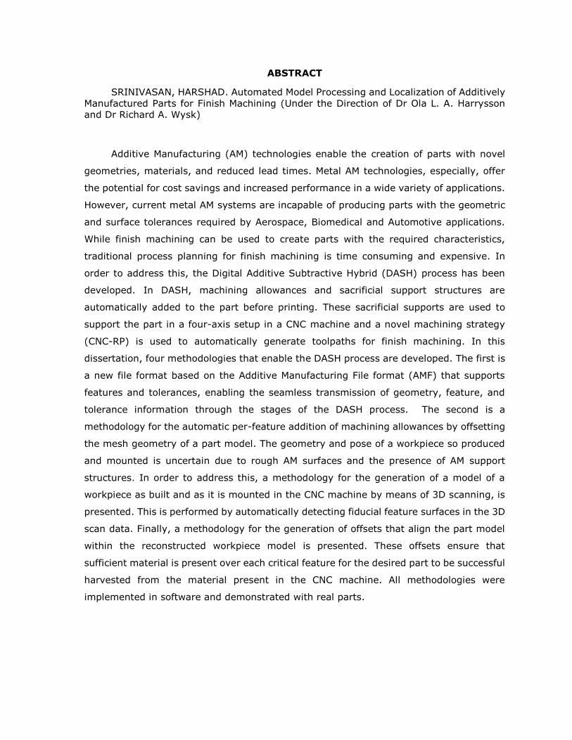
ABSTRACT

SRINIVASAN, HARSHAD. Automated Model Processing and Localization of Additively

Manufactured Parts for Finish Machining (Under the Direction of Dr Ola L. A. Harrysson and Dr Richard A. Wysk)

Additive Manufacturing (AM) technologies enable the creation of parts with novel

geometries, materials, and reduced lead times. Metal AM technologies, especially, offer

the potential for cost savings and increased performance in a wide variety of applications.

However, current metal AM systems are incapable of producing parts with the geometric

and surface tolerances required by Aerospace, Biomedical and Automotive applications.

While finish machining can be used to create parts with the required characteristics,

traditional process planning for finish machining is time consuming and expensive. In

order to address this, the Digital Additive Subtractive Hybrid (DASH) process has been

developed. In DASH, machining allowances and sacrificial support structures are

automatically added to the part before printing. These sacrificial supports are used to

support the part in a four-axis setup in a CNC machine and a novel machining strategy

(CNC-RP) is used to automatically generate toolpaths for finish machining. In this

dissertation, four methodologies that enable the DASH process are developed. The first is

a new file format based on the Additive Manufacturing File format (AMF) that supports

features and tolerances, enabling the seamless transmission of geometry, feature, and

tolerance information through the stages of the DASH process. The second is a

methodology for the automatic per-feature addition of machining allowances by offsetting

the mesh geometry of a part model. The geometry and pose of a workpiece so produced

and mounted is uncertain due to rough AM surfaces and the presence of AM support

structures. In order to address this, a methodology for the generation of a model of a

workpiece as built and as it is mounted in the CNC machine by means of 3D scanning, is

presented. This is performed by automatically detecting fiducial feature surfaces in the 3D

scan data. Finally, a methodology for the generation of offsets that align the part model

within the reconstructed workpiece model is presented. These offsets ensure that

sufficient material is present over each critical feature for the desired part to be successful

harvested from the material present in the CNC machine. All methodologies were

implemented in software and demonstrated with real parts.

© Copyright 2016 by Harshad Srinivasan

All Rights Reserved

Automated Model Processing and Localization of Additively Manufactured Parts

for Finish Machining

by

Harshad Srinivasan

A dissertation submitted to the Graduate Faculty of

North Carolina State University

in partial fulfillment of the

requirements for the degree of

Doctor of Philosophy

Industrial and Systems Engineering

Raleigh, North Carolina

2016

APPROVED BY:

_______________________________ _______________________________

Dr Ola L. A. Harrysson Dr Richard A. Wysk

Committee Chair

_______________________________ _______________________________

Dr Gregory D. Buckner Dr Ronald L. Aman

ii

DEDICATION

For Divya, who kept me

iii

BIOGRAPHY

Harshad Srinivasan was born in Chennai (Madras), Tamil Nadu, India. He earned his

Bachelors in Technology in (B.Tech) in Instrumentation and Control Engineering at the

National Institute of Technology, Tiruchirappalli (Trichy) in 2009. He attended graduate

school at North Carolina State University, where he earned a Masters (MS) in Mechanical

Engineering with a focus on Mechatronics and Control Systems in 2011. Subsequent to

this he enrolled in the doctoral program at Industrial and Systems Engineering at NCSU,

with a focus on Process Planning, Computational Geometry and Additive Manufacturing.

iv

ACKNOWLEDGMENTS

This work would not have been possible without the support of my family, friends

and colleagues. I would like especially thank my parents, Subhashini and V.R. Srinivasan,

who taught me the joys of learning and constantly encouraged and supported me through

this journey. I could not have gotten through this without Divya, my fiancé, who has

always been there to hold me up through the bad times and share in every moment of

joy.

I would like to express my gratitude to my advisor Dr. Ola Harrysson, and Dr Richard

Wysk for supporting my work and for giving me this opportunity. I would also like to thank

them and for their patience and for their guidance as I developed as a researcher. I would

like to thank Dr Ron Aman, Dr. Tim Horn, Dr. Harvey West and many others for all the

conversations, discussions, insights and help. Finally, I have to acknowledge the enormous

support I have received from my colleagues - the students and staff of CAMAL, NCSU;

they do amazing things every day.

This work would not have been possible without the support of the National Science

Foundation and America Makes / NCDMM.

v

TABLE OF CONTENTS

1. INTRODUCTION ....................................................................................... 1

1.1 Background .......................................................................................... 1

1.1.1 Additive manufacturing: ................................................................ 1

1.1.2 Hybrid manufacturing .................................................................... 3

1.1.3 CNC-RP ....................................................................................... 5

1.1.4 The DASH Approach ...................................................................... 7

1.2 Motivation ............................................................................................ 8

1.2.1 File formats and digital representation ............................................. 8

1.2.2 Automatic generation of machining allowances ................................. 8

1.2.3 Registration of sensor data............................................................. 9

1.2.4 Automatic generation of machining offsets ..................................... 10

1.2.5 Other challenges that must be addressed by DASH ......................... 10

1.3 Summary and overview of dissertation structure ..................................... 11

1.4 Chapter Bibliography ............................................................................ 13

2. LITERATURE REVIEW ............................................................................ 16

2.1 Rapid Prototyping and Additive Manufacturing ......................................... 16

2.1.1 Vat Polymerization ...................................................................... 16

2.1.2 Binder Jetting ............................................................................. 17

2.1.3 Powder Bed Fusion ...................................................................... 17

2.1.4 Material Jetting ........................................................................... 18

2.1.5 Material extrusion ....................................................................... 18

2.1.6 Directed energy deposition ........................................................... 19

2.1.7 Sheet lamination ......................................................................... 19

2.2 Additive manufacturing of metals........................................................... 20

2.2.1 Powder bed fusion processes ........................................................ 21

vi

2.2.2 Binder jetting processes............................................................... 24

2.2.3 Directed energy processes ........................................................... 27

2.2.4 Laminated object manufacturing ................................................... 29

2.3 Indirect manufacture of metal parts by additive manufacturing ................. 29

2.3.1 Additive manufacture of patterns for investment casting .................. 30

2.3.2 Direct production of molds using additive manufacturing ................. 31

2.4 Hybrid manufacturing ........................................................................... 31

2.4.1 Hybrid material deposition / subtraction in CNC machines ................ 32

2.4.2 Hybrid manufacturing by with other additive processes .................... 36

2.4.3 Hybrid manufacturing by stacking of machined sections ................... 36

2.5 Automatic workpiece sensing and 3D Scanning ........................................ 37


3. AMF FILE FORMAT WITH EXTENSIONS FOR GD&T ................................. 58

3.1 Background ........................................................................................ 58

3.1.1 File formats and their role in manufacturing ................................... 58

3.1.2 The AMF format .......................................................................... 62

3.1.3 Features and Tolerances .............................................................. 66

3.2 Literature Review ................................................................................ 67

3.2.1 Analysis of requirements .............................................................. 67

3.2.2 Approaches toward the solution and allied works ............................ 71

3.3 Synthesis of requirements .................................................................... 73

3.4 Proposed structure of Feature and Tolerance extensions to AMF ................ 75

3.4.1 Feature designation ..................................................................... 76

3.4.2 Feature Properties ....................................................................... 78

3.4.3 Tolerance information .................................................................. 79

3.4.4 Nominal size............................................................................... 83

3.4.5 Elements added to the AMF Specification ....................................... 84

3.5 Example implementation ...................................................................... 85

vii

3.6 Observations ....................................................................................... 86

3.6.1 Future developments ................................................................... 88

3.7 Conclusions ......................................................................................... 90


4. AUTOMATIC MESH OFFSET FOR THE GENERATION OF MACHINING

ALLOWANCES ......................................................................................... 96

4.1 Background and Motivation ................................................................... 96

4.2 Literature review ................................................................................. 98

4.2.1 Machining allowance by mesh offset .............................................. 98

4.2.2 Other approaches to machining allowance in Hybrid systems .......... 101

4.3 Problem description ........................................................................... 102

4.4 Methodology ..................................................................................... 103

4.4.1 Procedure for computing vertex displacement vector ..................... 105

4.4.2 Procedure for detecting and filling edges ...................................... 107

4.4.3 Implementation ........................................................................ 109

4.5 Observations, future work, and conclusions .......................................... 113

4.6 Chapter Bibliography .......................................................................... 115

5. AUTOMATIC REGISTRATION OF SCAN DATA TO MACHINE

COORDINATE SYSTEM .......................................................................... 116

5.1 Background ...................................................................................... 116

5.1.1 Part localization ........................................................................ 116

5.1.2 Current in-machine sensing systems ........................................... 118

5.1.3 Three dimensional scanning ....................................................... 119

5.2 Literature Review .............................................................................. 120

5.2.1 Scan matching systems ............................................................. 120

5.2.2 Registration of point cloud data to a defined coordinate system ...... 121

5.2.3 Automatic estimation of scanner pose ......................................... 122

5.2.4 Summary ................................................................................. 123

viii

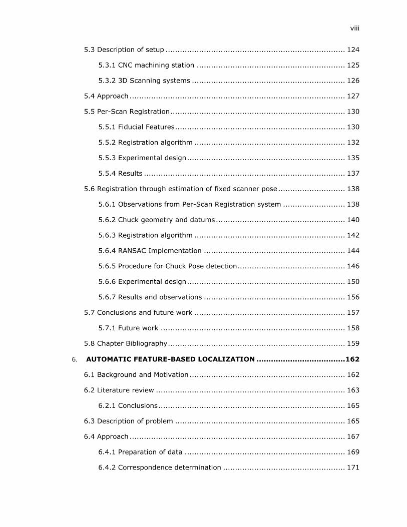
5.3 Description of setup ........................................................................... 124

5.3.1 CNC machining station .............................................................. 125

5.3.2 3D Scanning systems ................................................................ 126

5.4 Approach .......................................................................................... 127

5.5 Per-Scan Registration ......................................................................... 130

5.5.1 Fiducial Features ....................................................................... 130

5.5.2 Registration algorithm ............................................................... 132

5.5.3 Experimental design .................................................................. 135

5.5.4 Results .................................................................................... 137

5.6 Registration through estimation of fixed scanner pose ............................ 138

5.6.1 Observations from Per-Scan Registration system .......................... 138

5.6.2 Chuck geometry and datums ...................................................... 140

5.6.3 Registration algorithm ............................................................... 142

5.6.4 RANSAC Implementation ........................................................... 144

5.6.5 Procedure for Chuck Pose detection ............................................. 146

5.6.6 Experimental design .................................................................. 150

5.6.7 Results and observations ........................................................... 156

5.7 Conclusions and future work ............................................................... 157

5.7.1 Future work ............................................................................. 158


6. AUTOMATIC FEATURE-BASED LOCALIZATION ..................................... 162

6.1 Background and Motivation ................................................................. 162

6.2 Literature review ............................................................................... 163

6.2.1 Conclusions .............................................................................. 165

6.3 Description of problem ....................................................................... 165

6.4 Approach .......................................................................................... 167

6.4.1 Preparation of data ................................................................... 169

6.4.2 Correspondence determination ................................................... 171

ix

6.4.3 Optimization ............................................................................. 174

6.4.4 Overall localization approach ...................................................... 177

6.5 Example ........................................................................................... 179

6.6 Observations, conclusions and future work ........................................... 181


7. SOFTWARE SYSTEMS ........................................................................... 185

7.1 AMFCreator ....................................................................................... 185

7.1.1 AMFCreator UI .......................................................................... 185

7.1.2 Creating an AMF File ................................................................. 186

7.1.3 Creation and management of features ......................................... 188

7.1.4 Triangle selection ...................................................................... 190

7.1.5 Volume management ................................................................ 192

7.1.6 Computation of feature parameters ............................................. 193

7.1.7 Addition of machining allowances ................................................ 194

7.1.8 Creation of sacrificial support geometry ....................................... 195

7.2 SCANUI ............................................................................................ 198

7.2.1 Scan management .................................................................... 199

7.2.2 Interface with FARO scanner ...................................................... 201

7.2.3 Interface with CNC Machine ....................................................... 203

7.2.4 Registration ............................................................................. 204

7.2.5 Localization .............................................................................. 207

7.3 Conclusions ....................................................................................... 211


8. SUMMARY AND FUTURE WORK ............................................................ 213

x

LIST OF TABLES

Table 2.1: Parameters for some direct-metal powder-bed systems ............................ 26

Table 3.1: AMF-TOL Elements. .............................................................................. 84

Table 5.1: Experimental results. XM etc refer to measured (true) coordinates while

XL etc refer to the coordinates as located by the scan based localization

system. All units are in mm ............................................................... 138

Table 5.2: Mean system performance .................................................................. 138

Table 5.3: Parameters of test system .................................................................. 156

Table 5.4: Test runs. ......................................................................................... 156

xi

LIST OF FIGURES

Figure 1.1: CNC-RP process. (a) shows CNC-RP setup (b1-b4) show creation of

part and (b5-b6) show creation and removal of supports. Reproduced

with permission from [23]. .................................................................... 6

Figure 1.2: The DASH process sequence. ................................................................. 7

Figure 2.1 : Tree of Metal AM processes ................................................................. 21

Figure 2.2 : EOS M280 SLM system. Installed at CAMAL, North Carolina State

University.......................................................................................... 23

Figure 2.3: Concept Laser M2 Systems, Installed at Lawrence Livermore National

Labs ................................................................................................. 23

Figure 3.1: Core structure of the AMF document – showing geometry, material

specification and metadata .................................................................. 65

Figure 3.2: AMF triangle, designated as a part of a feature with id ‘2’ ........................ 76

Figure 3.3: Features by assigning feature id to triangles. Also shown is the

designation of a single feature across multiple volumes .......................... 77

Figure 3.4: XML of AMF with <features>, <feature>, id and feature information.

Extensions to AMF are shown in Red ..................................................... 78

Figure 3.5: Basic Anatomy of a feature control frame per ASME Y14.5 2009 ............... 79

Figure 3.6: Interpretation of tolerance zone from <maximum> and <minimum>

tags. Top showing interpretation if both tags are present, bottom

showing interpretation if <minimum> is omitted .................................... 81

Figure 3.7: Cylinder feature showing callout examples ............................................. 82

Figure 3.8: UML of AMF-TOL. Extensions to AMF standard highlighted in Red .............. 85

Figure 3.9: AMF Creator software showing ability to manipulate AMF-TOL files ............ 86

Figure 4.1: Projection of displacement vector onto incident triangle normals............... 99

Figure 4.2: Scheme for displacement of vertices presented by Qu and Stucker ......... 100

Figure 4.3: Offset with multiple features .............................................................. 102

Figure 4.4: Stitching edges together to form a closed volume ................................. 103

xii

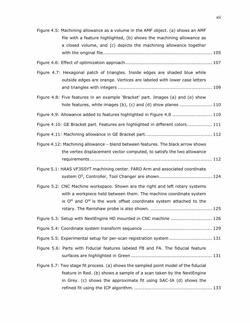
Figure 4.5: Machining allowance as a volume in the AMF object. (a) shows an AMF

file with a feature highlighted, (b) shows the machining allowance as

a closed volume, and (c) depicts the machining allowance together

with the original file .......................................................................... 105

Figure 4.6: Effect of optimization approach ........................................................... 107

Figure 4.7: Hexagonal patch of triangles. Inside edges are shaded blue while

outside edges are orange. Vertices are labeled with lower case letters

and triangles with integers ................................................................ 109

Figure 4.8: Five features in an example ‘Bracket’ part. Images (a) and (e) show

hole features, while images (b), (c) and (d) show planes ...................... 110

Figure 4.9: Allowance added to features highlighted in Figure 4.8 ........................... 110

Figure 4.10: GE Bracket part. Features are highlighted in different colors ................. 111

Figure 4.11: Machining allowance in GE Bracket part. ............................................ 112

Figure 4.12: Machining allowance – blend between features. The black arrow shows

the vertex displacement vector computed, to satisfy the two allowance

requirements ................................................................................... 112

Figure 5.1: HAAS VF3SSYT machining center. FARO Arm and associated coordinate

system OS, Controller, Tool Changer are shown.................................... 124

Figure 5.2: CNC Machine workspace. Shown are the right and left rotary systems

with a workpiece held between them. The machine coordinate system

is OM and OW is the work offset coordinate system attached to the

rotary. The Renishaw probe is also shown. .......................................... 125

Figure 5.3: Setup with NextEngine HD mounted in CNC machine ............................ 126

Figure 5.4: Coordinate system transform sequence ............................................... 129

Figure 5.5: Experimental setup for per-scan registration system ............................. 131

Figure 5.6: Parts with Fiducial features labeled FB and FA. The fiducial feature

surfaces are highlighted in Green ....................................................... 131

Figure 5.7: Two stage fit process. (a) shows the sampled point model of the fiducial

feature in Red. (b) shows a sample of a scan taken by the NextEngine

in Grey. (c) shows the approximate fit using SAC-IA (d) shows the

refined fit using the ICP algorithm. ..................................................... 133

xiii

Figure 5.8: Per-Scan registration algorithm flowchart ............................................ 134

Figure 5.9: Test workpiece. Image on right shows shims to simulate misalignment

as well as Renishaw probe, used to measure workpiece test surfaces. .... 135

Figure 5.10: Combined point cloud ...................................................................... 135

Figure 5.11: Test workpiece with reference surfaces highlighted in green. The

coordinate system OP is attached to and constructed from the

reference surfaces ............................................................................ 136

Figure 5.12: Sequence of steps used to create a combined model of the test

workpiece and to extract its true position in the CNC machine ............... 137

Figure 5.13: Effect of fiducial feature location and orientation error. The ‘FE’ and

‘WE’ superscripts refer to a fiducial feature location error and

workspace coordinate system error. ................................................... 139

Figure 5.14: Chuck and axes .............................................................................. 140

Figure 5.15: Chuck datums. The Chuck Body Cylinder is the primary Datum,

colored Red; The Chuck Face is the secondary datum, in green; Jaw

#1 Face is tertiary datum, colored blue. Jaws #2 and #3 are hidden,

for clarity ........................................................................................ 141

Figure 5.16: Algorithm for chuck pose extractions ................................................. 147

Figure 5.17: Example scan of chuck with 1.07 million points. .................................. 148

Figure 5.18: Rejection of ‘bad’ regions. Regions circled in white represent regions

on the datum surfaces where points were rejected by the RANSAC

system............................................................................................ 149

Figure 5.19: Extracted Datums. Chuck Body Cylinder in Red, Chuck Face in Green

and Jaw in Blue. ............................................................................... 149

Figure 5.20: Procedure for measuring the accuracy with which a chuck is located.

True axis and Expected planes are shown in green, the measured axis

and planes as produced are shown in orange ....................................... 150

Figure 5.21: FARO Edge with Mazak CNC machine and Chuck ................................. 152

Figure 5.22: Chuck and Jaws; Scanned at 0, 60 and 240 degrees ........................... 153

Figure 5.23: Scans at the three angles ................................................................. 153

xiv

Figure 5.24: Combined model of Jaw #2, Registered to the chuck coordinate

system............................................................................................ 154

Figure 5.25: Fitting of parallel planes to Jaw in Geomagic Qualify 2013 .................... 155

Figure 6.1: Depiction of localization problem. Blue dots depict the 3D scanned

measurements of the workpiece as built and as mounted. The arrows

attached to each point show the normal direction, oriented ‘outwards’.

The nominal part pose is shown in Orange, the Optimal part pose is

shown in Green and an infeasible pose is shown dashed in purple.

Coordinate system shown as per convention – Blue is Z axis and X is

in Red. ............................................................................................ 167

Figure 6.2: Down-sampling. From left to right we have the initial cloud, the grid

and the final selected points. The output points are selected from the

grid boxes with more than a threshold number of points (3, in this

case), shown in Green. Red boxes were rejected and white boxes were

never constructed as they contain no points. ....................................... 170

Figure 6.3: Projection based correspondence estimation. The dashed lines are rays,

oriented along the point normal, from the point to the nearest triangle

...................................................................................................... 171

Figure 6.4: Ray-triangle intersection. Projection vectors are collinear with the point

normal. The projected points lie on the triangle plane, either inside or

outside the triangle. ......................................................................... 172

Figure 6.5: Rejected correspondences. Point (a) is rejected as its angle is too

‘shallow’. (b) is rejected as it lies further away than a specified distance

from the triangle (c) is rejected as its normal is not aligned with the

triangle ........................................................................................... 173

Figure 6.6: Point-triangle correspondence computation. Each set of braces

represents a (nested) loop. ............................................................... 174

Figure 6.7: Error function in solid blue. The Cutoff is the intercept on the Distance

Axis, representing a triangle point distance equal to the desired

allowance. The dashed blue line represents the error function without

the cutoff. ....................................................................................... 176

Figure 6.8: Error function logic. The horizontal axis is point-surface distance and

the vertical axis is the error ............................................................... 177

xv

Figure 6.9: Best-Fit system UI ............................................................................ 179

Figure 6.10: Fit steps. (a) shows initial displacement, (b), (c) and (d) show the

alignment after 1, 2 and 3 iterations respectively ................................. 180

Figure 6.11: Fit statistics .................................................................................... 181

Figure 7.1: AMFCreator software. Major sections are labeled .................................. 186

Figure 7.2: Creating and selecting an object ......................................................... 187

Figure 7.3: Tasselated geometry imported as volume ............................................ 188

Figure 7.4: Adding features ................................................................................ 188

Figure 7.5: Feature controls ............................................................................... 189

Figure 7.6: Selection parameter controls .............................................................. 190

Figure 7.7: Effect of selection angle threshold. Same triangle clicked in all cases. ..... 191

Figure 7.8: Volume management. Seen is volume list with selected volume.

Selected volume highlighted in the display window. .............................. 192

Figure 7.9: Volume visibility dialog box. ............................................................... 192

Figure 7.10: Cylinder feature and extracted parameters. Parameters displayed as

metadata ........................................................................................ 194

Figure 7.11: Addition of machining allowances. Resulting allowance highlighted in

display window. ............................................................................... 194

Figure 7.12: Support geometry generation stages. (a) is initial geometry (b)

transformation to manufacturing position (c) support struts (d)

fixturing features ............................................................................. 196

Figure 7.13: Support Generation UI ..................................................................... 197

Figure 7.14: SCANUI interface elements .............................................................. 198

Figure 7.15: Point cloud on right created by clipping the point cloud on the left ........ 199

Figure 7.16: Down-sampling of scans .................................................................. 200

Figure 7.17: Faro scanner control options ............................................................. 201

Figure 7.18: Meshing of point cloud ..................................................................... 201

Figure 7.19: Approximate point normal ................................................................ 202

xvi

Figure 7.20: Serial port controls .......................................................................... 204

Figure 7.21: Registration parameters ................................................................... 205

Figure 7.22: Stitching scans together. Shown are the combined extracted datums

and four scans to be stitched together. ............................................... 206

Figure 7.23: Combined, registered scan ............................................................... 207

Figure 7.24: Localization controls ........................................................................ 208

Figure 7.25: Model with selected features highlighted ............................................ 209

Figure 7.26: Features to use ............................................................................... 209

Figure 7.27: Fit and associated statistics .............................................................. 210

1

Chapter 1

INTRODUCTION

This chapter presents a brief introduction to additive and hybrid manufacturing, their

advantages, shortcomings and associated challenges. The additive manufacture of metals

is briefly explored and hybrid manufacturing, as a possible solution to the shortcomings

of direct additive metal fabrication, is introduced. Specifically, a hybrid manufacturing

system is described in which existing additive and subtractive systems are tied together

using software (Digital Additive and Subtractive Hybrid manufacturing or DASH system).

The challenges associated with this system are briefly explored. Four specific requirements

of the DASH process are identified and approaches to address these challenges are

outlined. Finally, the structure of the rest of this dissertation is provided.

1.1 Background

1.1.1 Additive manufacturing:

Additive manufacturing (AM) is defined by the American Society for Testing and

Materials as “A process of joining materials to make objects from 3D model data, usually

layer upon layer, as opposed to subtractive manufacturing methodologies” [1]. The origins

of modern Additive Manufacturing technology can be traced to the rapid prototyping (RP)

systems first developed in the 1980s. Unlike RP systems, that have been are used to

produce prototypes for fit testing and visual evaluation, AM systems are focused on the

creation of functional net-shape or near-net-shape parts.

Similar to rapid prototyping, additive manufacturing involves the production of parts

layer by layer, with each layer forming a cross section of the part. To form a layer, material

is deposited on the previous layer and fused to it by the application of energy – thermal,

2

chemical or mechanical. This process – the production of parts by the addition of material,

as opposed to material removal, deformation or solidification as in traditional

manufacturing, gives additive manufacturing its name.

In general, AM systems do not require tooling or significant process planning. The

geometric constraints imposed by additive manufacturing methods are far less stringent

than traditional manufacturing methods- allowing for internal cooling channels,

functionally graded structures and non-stochastic mesh structures [2] [3] [4]. Several

additive manufacturing methods also permit the use of materials that are difficult to

process with traditional manufacturing methods such as superalloys and amorphous

metals [5] [6]. Several studies have also indicated that additive manufacturing systems

feature lower levels of material wastage than traditional manufacturing, that is - they

feature a high 'buy-to-fly' ratio. This measure is one that has grown from the aerospace

industry, where it is not unusual to machine away as much as 80% of the material from

raw stock.

AM systems also suffer from several drawbacks. The processing time per part with

additive manufacturing is usually far longer than in traditional methods. The raw materials

used for AM systems also tend to be more expensive and difficult to handle than the

equivalent raw stock used by traditional manufacturing systems [7]. Historically, additive

processes could not match the material properties (density, porosity, crystal structure) of

parts produced by traditional means, e.g. forgings or castings, nor the accuracy of CNC

machining. However significant progress in addressing material deficiencies has been

made in recent years, to the extent that additively produced metal parts now regularly

exceed the material performance of those made by traditional means [8] [9].

These factors render additive manufacturing well suited for the production of high

performance parts which feature novel materials and geometries, and/or parts for which

the small lot requirements make tooling per part very expensive. Examples include

3

medical devices that are customized to the patient, aerospace parts where performance

is paramount and legacy replacement parts for which tooling would otherwise have to be

re-created. These attributes have sparked significant interest in using additive

manufacturing in the aerospace, automobile, medical device, and tool and die industries.

The market for Additive manufacturing in 2012 was estimated at $2.204 billion with a

growth rate of 28.6% [10] with additive manufacturing of metals estimated at a $24.9

million and a growth rate of 38.3%. More recently, General Electric has earmarked $3.5

Billion for investment into additive manufacturing, indicating strong interest in additive

manufacturing from major corporations [11] [12].

The additive manufacture of metal parts holds special interest [13] as metals and

metal alloys are among the most important classes of engineering material in use today.

However, direct metal-AM parts possess surfaces that can be distorted by internal

stresses, witness marks from the removal of support structures and high surface

roughness [2], [14], [15]. Parts produced by indirect metal AM methods- either by

investment casting with additively produced patterns or by casting in additively produced

molds require the removal of runners, gate and vents and have to be finish machined in

order to achieve required dimensional accuracy. This is in addition to the “stair-stepping”

inherent in layer based manufacturing. Therefore, as with traditionally produced near-net-

shape parts; subtractive finish machining is required before additively produced parts can

be utilized. This process – the production of near-net-shape parts by additive means

followed by subtractive finishing using CNC machining comes under the ambit of the term

'Hybrid Manufacturing'.

1.1.2 Hybrid manufacturing

Hybrid manufacturing is a term that covers systems that combine more than one

type of manufacturing processes for the same part, to create the desired form [16]. Here,

4

we restrict the use of the term 'hybrid manufacturing' to refer to the finish machining of

parts produced by additive manufacturing.

In order to meet required form and dimensional tolerances, near-net-shape parts

require finish machining. Parts are finished by mounting them in a CNC machining station,

which is then used to machine away excess material and create critical mating and contact

surfaces etc. The near-net-shape part is designed with 'overgrown surfaces' to ensure

enough excess material is present for the successful creation of these critical surfaces.

Adopting this strategy with additively produced parts incurs several of the same drawbacks

that additive manufacturing seeks to avoid. Parts to be finished must be precisely located

in the CNC machine coordinate system. This is performed by either 1) mounting parts in

a series of specially designed fixtures, or 2) by manual positioning and offsetting the part

using probes and indicators, an operation that takes considerable time and skill. Carefully

designed and optimized machining tool-paths must also be developed to produce parts in

this manner. These strategies run counter to the use-case for AM- where low fixed costs

process and production engineering are followed by short lead times.

Several attempts have been made to address this challenge by integrating the

additive and subtractive sub-systems into a single machine such as the Matsuura Lumex

advance-25 [17]. The subtractive system is used to machine the periphery and/or face of

each layer, as they are created. This approach, however, requires that a complete system

be developed and deployed, representing significant capital costs. Other systems attempt

to simplify and reduce costs by retrofitting existing CNC systems with additive capability,

for example the HLM system [18] developed at the Indian Institute of Technology (IIT),

Bombay and the laser cladding system developed by Hybrid Manufacturing Technologies

[19]. Approaches of this nature appear incapable of generating many of the more complex

geometries that make additive manufacturing so attractive [20].

5

In order to circumvent these limitations while maintaining the best attributes of both

additive and subtractive manufacturing, it is desirable to utilize existing, proven, additive

and subtractive machines and tie them together using intelligent part design, sensing and

software. Such a system would minimize the need for manual intervention in fixture design

and tool-path planning for the finish machining. Such a system is the goal of the DASH

system.

1.1.3 CNC-RP

CNC-RP is a CNC-machining-based rapid prototyping system [21]. In CNC-RP, bar-

stock is held between centers (in a 3 jaw chuck or similar system) in the CNC machining

station such that it can be rotated (indexed) and machined from multiple orientations. At

each orientation, the CNC machine is used to create all accessible part surfaces. This is

performed by “island milling” - removing material layer by layer. Once all surfaces

accessible at a particular orientation have been created, the bar stock is rotated to the

next computed orientation and the process is repeated, creating those surfaces now

accessible. This is repeated until all part surfaces have been created. Given a target part

file, the CNC-RP software system computes the minimum diameter needed for the bar

stock, the set of angles from which all part surfaces are accessible ('visible') and machining

tool-paths for each angle. The tool-paths are generated by a commercial CAM system,

integrated into the CNC-RP software.

This approach reduces tool-path generation to a set of '2 ½' axis problems, for which

existing automatic tool path generators in commercial CAM software are sufficient. The

CNC-RP software also adds features to the part, in order to support it through the

machining operation(s), as the stock is machined away. The software designs these

supports to hold the part to within the minimum allowable deflection. After the process is

completed the supports are manually removed and any remaining witness marks are

buffed. The original CNC-RP software system required manual selection of an axis of

6

rotation. Extensions, to compute the optimal axis of rotation as well, have since been

studied [22]. Figure 1.1 illustrates the CNC-RP Process.

Figure 1.1: CNC-RP process. (a) shows CNC-RP setup (b1-b4) show

creation of part and (b5-b6) show creation and removal of supports.

Reproduced with permission from [23].

7

1.1.4 The DASH Approach

The Digital Additive Subtractive Hybrid (DASH) system extends CNC-RP to the

automatic finishing of additively manufactured parts. In DASH, (sacrificial) support

features are automatically added to the part before production in an existing additive

machine. In addition, prior to additive manufacture, the part is 'overgrown' (allowances

are added to the part) in order to compensate for inaccuracy in the additive and

subtractive systems. The sacrificial support features are used to mount the part in the

CNC machine, between centers. Subsequent to this, a measurement and sensing system

is used to determine the shape, form and position of the material actually present in the

CNC machine. Finally, A CNC-RP-like software system is used to automatically generate

the set of angles for machining visibility and the finishing tool-paths at each indexed angle.

After the finish machining is completed, the sacrificial features are removed, either

manually or by the CNC machine, and any remaining witness marks manually finished.

Figure 1.2 shows the DASH process sequence.

Figure 1.2: The DASH process sequence.

8

This approach requires the development of several new technologies and

methodologies. The necessity for these methodologies, forms the motivation for this

dissertation.

1.2 Motivation

The DASH process provides a path towards the automatic production of parts which

feature both the materials and geometries enabled by additive manufacturing as well as

the accurate surfaces and features required for many applications. However, there are

several challenges with DASH, which must be addressed before it can be utilized at a

commercial level. This dissertation is motivated by the need to address four specific

challenges.

1.2.1 File formats and digital representation

The DASH process involves the intelligent combination of additive and subtractive

manufacturing as well as in-process sensing together with several processing and planning

algorithms. In order to drive these systems, it is necessary to define a portable data format

that holds the required geometric, feature and tolerance information. Such a data format

will form the basis of information storage, retrieval and exchange between the various

modules that comprise the DASH system and ensure data portability as well as consistent

inputs to all systems. In addition, a proper data format will allow information exchange

with all potential stakeholders involved.

1.2.2 Automatic generation of machining allowances

Finish machining involves the removal of material from a workpiece, in order to

produce the required part, to the required tolerances. In order to be successful, the

workpiece must have sufficient excess material such that all desired part surfaces may be

found within it. In order to achieve this condition, machining allowance must be added to

the part model before the workpiece is produced by a near-net shape process.

9

In DASH, this must be performed automatically and on a per-feature basis, prior to

additive manufacture. Therefore, a system for altering the nominal part geometry

automatically by adding additional material for machining allowances on a per feature

basis to a part model, is necessary.

1.2.3 Registration of sensor data

Since the sacrificial support features used by the DASH process are produced by the

same additive process as the part, they feature similar rough, near-net-shape surfaces.

When these rough surfaces are used to clamp and locate the part in a fixture, the part

location becomes uncertain.

Additionally, in practice, those AM support structures which can easily be removed

are manually broken off before mounting in the CNC machine. Any tool-path designed to

machine away the maximum possible volume that these support structures may occupy

will spend a significant amount of time 'cutting air'.

The integration of a workpiece measurement and sensing system into the CNC

machine is a possible means to address these challenges. Such a system can be used to

generate a model of the part as-built and as it is mounted in the CNC machine. This model

may then be used to efficiently harvest the desired part from the material actually

present in the CNC machine.

Optical systems capable of capturing three dimensional data appear to be best suited

for the task in-machine workpiece sensing and workpiece model generation. These systems,

sometimes referred to using the term ’3D scanning’ consist of a family of technologies

that can capture three dimensional data of surfaces present in their field of view. 3D

scanning systems generate dense data – up to millions of points per scan. This enables

the detection of features and geometries that cannot be adequately detected by touch

probing.

10

However, scan data is produced in a frame of reference internal to the scanner. In

order to drive tool-path creation, this data must be transformed to the CNC coordinate

frame. Traditional methods for addressing this are impractical, inflexible and in many

cases cost-prohibitive.

In order to address this, a method for automatically transforming 3D scan data from

the scanner to machine coordinate systems is necessary.

1.2.4 Automatic generation of machining offsets

Finally, it is necessary to compute offsets that compensate for the difference

between the nominal part model and the model of the workpiece material as built and as

it is mounted in the CNC machine. These offsets must move the part ‘into’ the material

present, such that there is sufficient material present ‘above’ each feature for its successful

production. This offset generation system must be fast and capable of accommodating

arbitrary geometries.

1.2.5 Other challenges that must be addressed by DASH

In addition to the four challenges highlighted in sections 1.2.1 – 1.2.4, that are the

focus of this dissertation, there are several other challenges that must be addressed in

order for the successful manufacture of parts via the DASH process.

1.2.5.1 Selection of machining axis and strategy

Due to the limitations of tool access in CNC machining, only surfaces with a clear

line of sight can be finish-machined. This limits the ability of DASH to finish-machine part

surfaces when inaccessible geometries are present in the part. However, in most

'engineering' parts, the critical surface are external mating surfaces and finishing of non-

critical surfaces is secondary to accurately producing these, a task DASH is well suited for.

In order to successfully produce a part, it is important to ensure that all critical part

surfaces can be accessed by the CNC machine, that all surfaces requiring high surface

11

tolerance can be machined using an appropriate strategy and that mating surfaces are

not marred by the attachment of sacrificial fixturing features. This requires careful

selection of the axis of rotation and consequently, the selection of the attachment sites of

for the sacrificial supports.

For certain parts, it may be impossible to satisfy all the competing objectives

simultaneously. In these cases, it becomes necessary to select the most critical surfaces

and prioritize them for proper finish machining over less critical surfaces

1.2.5.2 Part and tool deflection under machining forces:

In the DASH approach (as in CNC-RP), the part is held between centers at opposite

ends, a configuration significantly less rigid than a part held in a traditional fixture. This

results in both static part deflection under machining forces and dynamic deflection

(vibration). In addition, the tools required by these machining strategies tend to be long

and feature small diameter-length aspect ratios. When machining tough materials, this

causes significant tool deflection and chatter, resulting in incomplete material removal and

poor surface and dimensional quality. These effects must be understood and accounted

for.

1.3 Summary and overview of dissertation structure

In this chapter, brief introductions to additive manufacturing, hybrid manufacturing

and the DASH system were presented. Four specific challenges that must be addressed in

order for the DASH system to meet its requirements were identified.

Chapter 2 presents a review of the literature and current state of additive

manufacturing and hybrid manufacturing. Chapter 3 describes the development of a file

format to address the needs of the DASH process by extending the AMF specification to

include features and tolerances. Chapter 4 describes a methodology for the automatic,

per-feature, generation of machining allowances by offsetting the mesh geometry of an

12

AMF file which includes demarcated features. Chapter 5 describes a methodology by which

the problem of registering scan data to the CNC machine work coordinate system is

addressed. This is performed by automatically detecting and measuring fiducial features

in the CNC machine workspace. These measurements are used to transform scan data in

order to create a model of the workpiece as built and as it is mounted in the CNC machine.

Chapter 6 presents a system for the automated computation of offsets to compensate for

deviations between the nominal part geometry and the scanned workpiece model. Chapter

7 contains descriptions and examples of the software systems that incorporate these

methodologies and integrate them into the unified DASH manufacturing system. Finally,

Chapter 8 contains a discussion and conclusion of the systems described and developed

in this dissertation, together with proposed avenues for future work.

Chapters 4 through 7 each contain an introduction to the problems they address, a

review of literature specifically connected with that problem, a description of the solution

approach, a section on testing and analysis and a conclusion section that includes

limitations, challenges and future work associated with each of these systems. In this way,

each chapter forms a self-contained research project while maintaining a coherent theme.

13

1.4 Chapter Bibliography

[1] A. Standard, “F2792. 2012. Standard Terminology for Additive Manufacturing

Technologies,” ASTM F2792-10e1.

[2] I. Gibson, Additive manufacturing technologies: rapid prototyping to direct digital

manufacturing. London ; New York: Springer, 2010.

[3] L. E. Murr, S. M. Gaytan, F. Medina, H. Lopez, E. Martinez, B. I. Machado, D. H.

Hernandez, L. Martinez, M. I. Lopez, R. B. Wicker, and J. Bracke, “Next-generation

biomedical implants using additive manufacturing of complex, cellular and functional

mesh arrays,” Philos. Trans. R. Soc. Math. Phys. Eng. Sci., vol. 368, no. 1917, pp.

1999–2032, Apr. 2010.

[4] L.-E. Rännar, A. Glad, and C.-G. Gustafson, “Efficient cooling with tool inserts

manufactured by electron beam melting,” Rapid Prototyp. J., vol. 13, no. 3, pp. 128–

135, Jun. 2007.

[5] L. E. Murr, S. M. Gaytan, D. A. Ramirez, E. Martinez, J. Hernandez, K. N. Amato, P.

W. Shindo, F. R. Medina, and R. B. Wicker, “Metal Fabrication by Additive

Manufacturing Using Laser and Electron Beam Melting Technologies,” J. Mater. Sci.

Technol., vol. 28, no. 1, pp. 1–14, Jan. 2012.

[6] G. P. Dinda, A. K. Dasgupta, and J. Mazumder, “Laser aided direct metal deposition

of Inconel 625 superalloy: Microstructural evolution and thermal stability,” Mater.

Sci. Eng. A, vol. 509, no. 1–2, pp. 98–104, May 2009.

[7] C. K. Chua, K. F. Leong, and C. S. Lim, Rapid prototyping: principles and applications.

World Scientific, 2010.

[8] E. C. Santos, M. Shiomi, K. Osakada, and T. Laoui, “Rapid manufacturing of metal

components by laser forming,” Int. J. Mach. Tools Manuf., vol. 46, no. 12–13, pp.

1459–1468, Oct. 2006.

[9] L. E. Murr, E. V. Esquivel, S. A. Quinones, S. M. Gaytan, M. I. Lopez, E. Y. Martinez,

F. Medina, D. H. Hernandez, E. Martinez, J. L. Martinez, S. W. Stafford, D. K. Brown,

T. Hoppe, W. Meyers, U. Lindhe, and R. B. Wicker, “Microstructures and mechanical

properties of electron beam-rapid manufactured Ti–6Al–4V biomedical prototypes

compared to wrought Ti–6Al–4V,” Mater. Charact., vol. 60, no. 2, pp. 96–105, Feb.

2009.

[10] T. T. Wohlers, Wohlers Report 2013: Additive Manufacturing and 3D Printing State

of the Industry: Annual Worldwide Progress Report. 2013.

14

[11] H. Smith, “3D Printing News and Trends: GE Aviation to grow better fuel nozzles

using 3D Printing.” .

[12] B. P. Conner, G. P. Manogharan, A. N. Martof, L. M. Rodomsky, C. M. Rodomsky, D.

C. Jordan, and J. W. Limperos, “Making sense of 3-D printing: Creating a map of

additive manufacturing products and services,” Addit. Manuf.

[13] “Layers of Complexity: Making the Promises Possible for Additive Manufacturing of

Metals,” JOM, pp. 1–14, Oct. 2014.

[14] M. B. Bauza, S. P. Moylan, R. M. Panas, S. C. Burke, H. E. Martz, J. S. Taylor, P.

Alexander, R. H. Knebel, R. Bhogaraju, M. T. O’Connell, and others, “Study of

accuracy of parts produced using additive manufacturing,” Lawrence Livermore

National Laboratory (LLNL), Livermore, CA, 2014.

[15] G. D. Kim and Y. T. Oh, “A benchmark study on rapid prototyping processes and

machines: quantitative comparisons of mechanical properties, accuracy, roughness,

speed, and material cost,” Proc. Inst. Mech. Eng. Part B J. Eng. Manuf., vol. 222, no.

2, pp. 201–215, Oct. 2008.

[16] Z. Zhu, V. G. Dhokia, A. Nassehi, and S. T. Newman, “A review of hybrid

manufacturing processes – state of the art and future perspectives,” Int. J. Comput.

Integr. Manuf., vol. 26, no. 7, pp. 596–615, 2013.

[17] “Matsuura Machinery Corporation｜LUMEX Avance-25.” [Online]. Available:

http://www.matsuura.co.jp/english/contents/products/lumex.html. [Accessed: 11-

Jun-2014].

[18] K. P. Karunakaran, S. Suryakumar, V. Pushpa, and S. Akula, “Low cost integration

of additive and subtractive processes for hybrid layered manufacturing,” Robot.

Comput.-Integr. Manuf., vol. 26, no. 5, pp. 490–499, Oct. 2010.

[19] “Hybrid Manufacturing Technologies | Technology,” Hybrid Manufacturing

Technologies. [Online]. Available:

http://www.hybridmanutech.com/technology.html. [Accessed: 14-Jun-2014].

[20] I. Kelbassa, T. Wohlers, and T. Caffrey, “Quo vadis, laser additive manufacturing?,”

J. Laser Appl., vol. 24, no. 5, p. 050101, Nov. 2012.

[21] M. C. Frank, R. A. Wysk, and S. B. Joshi, “Rapid planning for CNC milling—A new

approach for rapid prototyping,” J. Manuf. Syst., vol. 23, no. 3, pp. 242–255, 2004.

15

[22] Y. Li and M. C. Frank, “Computing Axes of Rotation for Setup Planning Using Visibility

of Polyhedral Computer-Aided Design Models,” J. Manuf. Sci. Eng., vol. 134, no. 4,

pp. 041005–041005, Jul. 2012.

[23] Joseph E. Petrzelka and Matthew C. Frank, “Advanced process planning for

subtractive rapid prototyping,” Rapid Prototyp. J., vol. 16, no. 3, pp. 216–224, Apr.

2010.

[24] D. R. McMurtry, “Contact-sensing probe,” 4155171, 22-May-1979.

[25] D. R. McMurtry, “Coordinate measuring machine,” 4333238, 08-Jun-1982.

16

Chapter 2

LITERATURE REVIEW

This chapter contains an overview of the literature pertinent to this dissertation.

Section 2.1 contains a very brief review of the history and classification of Rapid

Prototyping and Additive Manufacturing Technologies. Direct metal additive manufacturing

is a field of particular interest to this work, a review of the processes and research in this

field is presented in Section 2.2. Section 2.3 presents the developments and work in the

field of hybrid manufacturing. Finally, In-machine workpiece sensing and 3D scanning

technologies are reviewed in section 2.4. In addition to the information contained in this

chapter, chapters 4 through 8 contain reviews of the literature and state of the art directly

related to their specific research objectives.

2.1 Rapid Prototyping and Additive Manufacturing

The production of parts additively, layer by layer, was first described and patented

in the 1980s [1] by groups in several countries, including Japan, France and the USA. A

number of different approaches to rapid prototyping and additive manufacturing have

since been developed. These can be classified into categories based on the processes and

technologies involved, as in ASTM F2792 [2]:

2.1.1 Vat Polymerization

Vat Polymerization [2] systems involve the selective curing of liquid polymer in a

vat, usually by optical means. After a part cross section (layer) has been created (cured),

the layer is re-coated with polymer resin and the process is repeated. The first Vat

Polymerization system was SLA ('Steriolithography Apparatus'), patented by Charles Hull

in 1984 [3] and marketed by 3D systems. This was also the first commercial, additive,

free-form fabrication process. In SLA, the photopolymer is 'cured' by means of a

17

galvanically steered laser spot. Modern developments include the use of micro mirror

arrays (DLP technology) [4] [5] [6] to project light patterns,[4] micro scale lithography

[7] [8] [9] and more sophisticated resins [10] [11] [12].

2.1.2 Binder Jetting

In Binder Jetting processes, layers are generated by selectively spraying a binder

onto a powder bed. The binder fuses the powder to form a solid layer. Once a layer is

created, the powder bed is lowered, re-coated with an even layer of powder and the

process is repeated to build up the object. The first binder jetting processes was '3D

printing', developed at MIT in 1989 [13] [14]]. Modern Binder Jetting processes can be

used to create plastics [4], composites [12] [15], ceramic [16], sand (for casting) [17]

[18] [19] [20] and metal parts [21] [22] [23]. This process is also capable of generating

full color parts, by using pigments along with the binder. Curing, infiltration and sintering

may be required after initial part production for the part to achieve its final strength and

surface characteristics [12] [21] [23].

2.1.3 Powder Bed Fusion

Powder Bed Fusion processes function similarly to binder jetting in that solid layers

are generated by fusing powder together, in a powder bed. In powder bed fusion, however,

the binding is achieved by application of thermal (in the form of focused energy) rather

than chemical energy. The first process of this type was Selective Laser Sintering (SLS),

developed in the late 1980s by Drs. Joseph Beaman and Carl Deckard and marketed by

the DTM corporation [24] [25] [24] (since then acquired by 3D Systems). The thermal

energy may cause either sintering as in SLS or complete melting as in Direct Metal Laser

Sintering [26] (DMLS), Selective Laser Melting [27] (SLM) and Electron Beam Melting

(EBM) processes [27] [28] [29]. Powder bed fusion can be used to generate

thermoplastics, ceramics and metals as well as composite materials (using mixed

18

powders) [4] [30] [31]. Lasers, focused light and Electron Beams have been used as

energy sources.

2.1.4 Material Jetting

In material jetting processes, droplets of material are sprayed from a nozzle (or

series of nozzles) in order to build up layers. The jetting may be achieved by piezoelectric,

thermal or by jetting in an aerosol form [32] [33]. Materials can include polymers

(including photopolymers), waxes (for investment casting), ceramics [34] and metals [1]

[4] [35]. If a photopolymer is employed, an appropriate light source adjacent to the

deposition head is used as a source of energy for curing. The first such devices were

manufactured and marketed by Solidscape Inc. (then known as Sanders Prototype) in

1994 [1]. More recently, this method has been extended to the direct production of

functionally graded and multi-material parts [36], electronic components that include both

conductive and insulating elements [37] [38] and weld based production of metal parts

using droplets of molten metal [39] [40] [41] [42].

2.1.5 Material extrusion

Material extrusion processes are among the most common solid free-form

fabrication systems in use today, representing the largest installed base [43]. In material

extrusion processes a continuous stream of material extruded from a nozzle is used to

build up part layers. The nozzle is moved relative to the build platform, in order to create

the layer geometry. The first material extrusion system, Fused Deposition Modeling (FDM)

was developed and patented by Scott Crump in 1989 [44]. FDM systems produce

thermoplastic parts by the extrusion of a stream of material heated to above its glass

transition temperature. Materials include a wide variety of engineering plastics such as

Nylon, ABS, PLA, Polycarbonate [45] and elastomers [46] [47]. Other materials that may

be processed by FDM style material extrusion include metals [48] and ceramics [49] [50]

by powder filled filament as well as composite material by filament containing reinforcing

19

fiber. Systems capable of extruding cement and high performance concrete [51] [52] [53],

bio-compatible materials [54] [55], food [56], and conductive elements [57] [58] have

also been developed.

2.1.6 Directed energy deposition

Directed energy deposition processes are similar to material jetting and material

extrusion is some respects. In directed energy deposition systems, focused thermal

energy is used to bond (by fusion or surface sintering) materials to the substrate (prior

layers or the build platform) in order to build up layers. The material may consist of a

continuous wire feed or powder carried by an inert gas [59] [60] [61]. The thermal energy

may be supplied by laser [62], electron beam [63] or plasma arc [64]. The first powder

based directed energy deposition systems was the LENS process developed at Sandia Labs

and marketed by Optomec [1] [65] [66]. These systems are primarily used to produce

metal parts, including high performance aerospace alloys [67], and are often used for

mold and part repair and re-manufacture [68]. Materials can include functionally graded

parts, produced by varying the material composition during the build [69].

2.1.7 Sheet lamination

Sheet lamination processes produce parts by fusing sheets of material one on top of

the other, forming a laminate. The cross section of the part (the layer shape) is cut out of

each sheet either after bonding (bond-then-form) or before bonding (form-then-bond) [1]

[4]. After production, the sections of the laminate not corresponding to the part are

broken off. The process of removing excess material may be assisted by the addition of a

hatch pattern in the excess material while the layer profile is also being created. The first

sheet lamination process, Laminated Object Manufacturing (LOM) can be credited to

Michael Feygin and Helisys Inc. (succeeded by Cubital Technologies) in 1985-86 [4] [70].

Sheets may be composed of metal [71], polymer, or paper [12] [72]. Cross sections may

be created by cutting with lasers or by mechanical means such as CNC milling or cutting

20

sheets with a blade. Bonding may be achieved chemically, thermally or by ultrasonic

welding.

2.2 Additive manufacturing of metals

The focus of this dissertation is the development of an automated system for the

finish machining of near-net-shape parts. The proposed system can be used with nearly

any such process, including traditional methods such as forging and casting. However,

economic and performance considerations limit its utility to the finish machining of parts

produced using additive manufacturing. The objective of this section is to describe the

state-of-the-art in Metal additive manufacturing with a focus on commercially available

systems. The Process capabilities, limitations, materials and other characteristics will be

briefly discussed. This will help form a map of additive manufacturing processes that can

be used to ‘drive’ the proposed system. Processes are grouped by the ASTM classification

from section 2.1. The final section - Indirect manufacture of metal parts by additive

manufacturing - contains a brief review of indirect metal part production methods – metal

parts produced using additively produced patterns for investment casting and direct

additive mold production for sand casting. Figure 2.1 : Tree of Metal AM processes shows

a tree of Metal AM processes.

21

2.2.1 Powder bed fusion processes

The first metal capable powder bed fusion process was Selective Laser Sintering

(SLS) [24], [25], [73]. In selective laser sintering, one or more lasers are used to bind

powdered material by selectively raising the local temperature [74]. This causes power

particles to bind by one of several mechanisms – (i) Solid State Sintering , (ii) Chemically

Induced Binding, (iii) Liquid Phase Sintering, and (iv) Full Melting [29] [75]. When Full

Melting occurs, the process is generally referred to as Selective Laser Melting (SLM). SLS

was first used to produce metal parts via the Liquid Phase Sintering process in which

binding is achieved by melting thermoplastic. The thermoplastic is either mixed in with

the metal powders or metal powder particles are coated in thermoplastic [76]. After

processing in the SLS system, the part is removed and thermally treated to burn off the

thermoplastic and sinter the metal powders, forming a partially dense metal part and in

some cases infiltrated to provide improved performance and density part [16] [77] [78]

[79] [80].

Figure 2.1 : Tree of Metal AM processes

22

Modern systems for the production of metal parts largely rely on the full melting and

direct bonding of power by higher power lasers. Examples include 3D System's Direct

Metal Printing (DMP) systems [81] [82], Renishaw's AM250 [83], SLM Solution's SLM

series [84], Concept Laser's Lasercusing systems [85] and the Direct Metal Laser Sintering

(DMLS) process by EOS GmbH [86].These systems directly process metal powders and

supply enough energy to either sinter or completely melt the functional metal powders

directly. It must be noted that many DMLS systems, despite the name, achieve full melting

[4] [87]]. Laser melting is considered superior to Laser sintering as it can be used to

produce parts with superior density and mechanical properties and requires less post

processing [88]. However, due to the high thermal gradients and considerable shrinkage

during the solid-liquid-solid transformation, significant internal stresses can arise,

potentially leading to distortions and cracks in the final part [89] [90] [91] [92]. This

necessitates the addition of support structures to hold the part in place against warping.

The removal of these support structures is laborious and time consuming. In addition, a

heat treatment process, such as hot iso-static pressing or annealing is required before the

part is removed from the build plate in order to prevent part distortion due to internal

stresses [1] [93] [94] [95].

The part is normally produced fused to the build platform. Separation from the

platform is performed by cutting the part off with a saw or by Wire-EDM. This must be

followed by removal of support structures and finish machining of surfaces and features

to specified critical tolerances or surface finish. The Matsuura Lumex 25 [96] is the

exception to this as it integrates both additive and subtractive subsystems into the same

volume. This allows additively produced layers to be finish machined as they are produced,

simplifying or completely eliminating the requirement for process planning and tooling for

finishing. Further processes of this kind will be discussed in section 2.3.

23

Electron Beam Melting (EBM) by Arcam is a powder-bed-fusion process similar to

Selective Laser Melting. However, in EBM the thermal energy is provided by an electron

beam generated by a heated tungsten filament and collimated, focused and guided by

Figure 2.3: Concept Laser M2 Systems, Installed at

Lawrence Livermore National Labs

Figure 2.2 : EOS M280 SLM system. Installed at

CAMAL, North Carolina State University

24

magnetic fields. Full melting and near 100% part densities are achieved [28] [97]. The

use of an electron beam provides certain advantages including higher scan rates (up to

10,000 m/s) [28] [98], higher beam power and efficiency [88] and associated higher build

rates compared to laser based processes [99], reduced internal stresses due to the

elevated build temperature [100] which in turn reduce the need for thermal post-

treatment and [28] allow less dense support structures than laser based melting

processes.

Conversely, the EBM process also has several deficiencies compared to SLM and

SLS. These include the need for processing under vacuum, increased cool-down time and

greater roughness on part surfaces together with greater difficulty in removing excess

powder, caused by partial sintering of powder under the elevated build temperature. With

alloys incorporating metals with low vaporization temperatures such as Al and Mg, the

high build temperature and low pressure in the build chamber may cause a fraction of

these metals to volatilize, changing the alloy composition. Changes in alloy composition

and process parameters are needed to minimize and compensate for this effect [101]

[102]. Another significant challenge with electron beam melting is the buildup of charge

on the powder bed. This charge must be dissipated before it forces the powder particles

apart (causing it to 'smoke'). This limits the use of electron beam melting to relatively

conductive materials and considerable care is required to ensure that a path for charge

dissipation and sufficient time before consecutive scans is always provided.

2.2.2 Binder jetting processes

Binder jetting processes may also be used for the direct production of metal parts

as in the ExOne process. In the ProMetal process by ExOne [103], a metallic powder (such

as 420, 316 stainless [103]) is bonded with the help of a resin solution. The resin is then

thermally cured to produce a green part. Early efforts resulted in green parts with densities

in the 40% - 60% range, approximately [21]. The green part is finally sintered at high

25

temperature and impregnated with Bronze, if necessary, resulting in a composite metal

with 95% [21] density. More recent systems are able to achieve 95% or greater density

after sintering, with no impregnation necessary.

The primary advantage of binder jetting is the lack of internal stresses as the

binding is performed by chemical rather than thermal means. This allows parts to be

produced without support structures and eliminates the labor associated with removing

the part from the build plate. However, the green part is fragile [88] and requires care

while handling and cleaning, resulting in relatively high failure rates in parts with

complicated, fragile structures. In addition, the extra steps required (binder curing and

solid state sintering + infiltration) dramatically increase the overall production time.

Powder bed processes, both fusion and binder jetting, are of particular interest to

this work as they are the most capable class of direct metal system in terms of possible

part complexity as well as adoption. They are the class of system most likely to form the

additive basis of the proposed system. In order to better understand the relative

capabilities of these systems, Table 2.1: Parameters for some direct-metal powder-bed

systems contains the reported performance and build parameters for several direct-metal

additive systems.

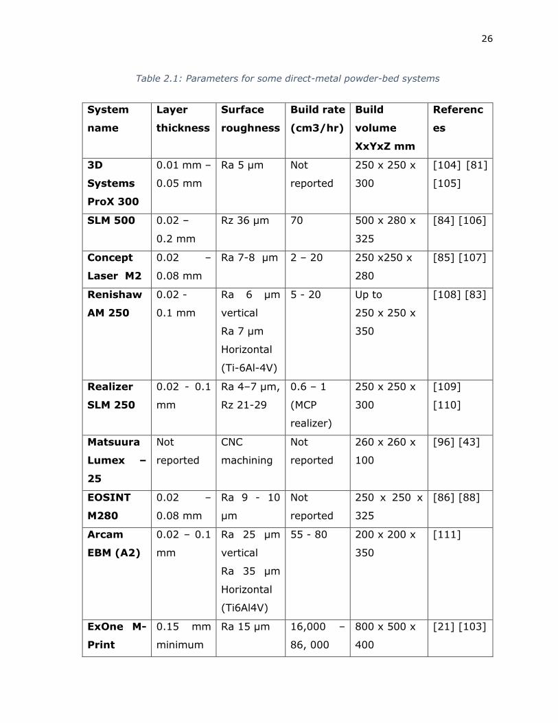
26

System

name

Layer

thickness

Surface

roughness

Build rate

(cm3/hr)

Build

volume

XxYxZ mm

Referenc

es

3D

Systems

ProX 300

0.01 mm –

0.05 mm

Ra 5 μm Not

reported

250 x 250 x

300

[104] [81]

[105]

SLM 500 0.02 –

0.2 mm

Rz 36 μm 70 500 x 280 x

325

[84] [106]

Concept

Laser M2

0.02 –

0.08 mm

Ra 7-8 μm 2 – 20 250 x250 x

280

[85] [107]

Renishaw

AM 250

0.02 -

0.1 mm

Ra 6 μm

vertical

Ra 7 μm

Horizontal

(Ti-6Al-4V)

5 - 20 Up to

250 x 250 x

350

[108] [83]

Realizer

SLM 250

0.02 - 0.1

mm

Ra 4–7 μm,

Rz 21-29

0.6 – 1

(MCP

realizer)

250 x 250 x

300

[109]

[110]

Matsuura

Lumex –

25

Not

reported

CNC

machining

Not

reported

260 x 260 x

100

[96] [43]

EOSINT

M280

0.02 –

0.08 mm

Ra 9 - 10

μm

Not

reported

250 x 250 x

325

[86] [88]

Arcam

EBM (A2)

0.02 – 0.1

mm

Ra 25 μm

vertical

Ra 35 μm

Horizontal

(Ti6Al4V)

55 - 80 200 x 200 x

350

[111]

ExOne M-

Print

0.15 mm

minimum

Ra 15 μm

16,000 –

86, 000

800 x 500 x

400

[21] [103]

Table 2.1: Parameters for some direct-metal powder-bed systems

27

2.2.3 Directed energy processes

Directed energy processes produce parts by fusing material to previously produced

layers (or to the build platform) by means of applied energy. The material can be supplied

by either a wire feed or as a powder in a carrier gas [59]. The energy source may take

the form of a Laser, Electron Beam or Plasma arc [62] [63] [64] [112].

Laser Directed energy deposition systems are related to laser cladding systems in

which a laser is used to produce a small melt pool on the substrate. Material is added to

the melt pool as a wire feed or by delivering metal powders in a carrier gas [113]. The

heat affected zone and global power input are small, leading to low overall heat distortions.

Laser cladding systems are used for both the production of near-net-shape parts and for

part repair [60] [114].

The laser cladding / directed energy deposition system(s) by Optomec [115],

referred to as Laser Engineered Net Shaping (LENS) is specifically designed for the

production of near net shape parts. In the LENS process material is delivered by co-axial

(to the laser head) feeding of metal powders in a carrier gas, allowing full 5 axis deposition

of material. In addition multiple materials may be fed in order to create functionally graded

parts with varying material and alloy compositions [116] [117] and the process may be

controlled for porosity and mechanical properties [118]. Material properties can match or

exceed the properties of traditionally produced parts [43] though other studies have

shown lower part strength compared to wrought parts [113]. Other laser based directed

energy deposition systems include the Direct Metal Deposition (DMD) process produced

by the POM group [119] and the EasyClad systems from BeAM systems [43] [120].

Several vendors of laser welding and cladding systems also market their products as being

capable of direct deposition manufacturing. Trumpf systems [121] produces systems

capable of additive part production as well as upgrade kits that enable additive part

production using systems originally designed for laser welding and cladding [43]. RPM

28

Innovations Inc. manufactures Laser deposition stations capable of cladding as well a

'Laser Freeform Manufacturing technology' (LFMT) [122]. These systems feature large

work envelopes, 3 – 4 kilowatt lasers and multiple powder feeds. Systems are also

manufactured by Mazak [123], MER [124], Irepa [125] and Huffman [126].

Laser based directed energy deposition systems are capable of producing surfaces

and material of comparable accuracy (50 to 100 µm) and roughness (near 10um Ra) to

SLS and SLM systems [127], though is subject to the specific materials and processes

used.

Plasma based directed energy deposition is largely confined to research applications.

Honeywell Aerospace manufactures a plasma based deposition system referred to as Ion

Fusion Formation (IFF) [43] [112] where the material is impelled into the workpiece by a

carrier gas plasma. The material is in the form of wire feedstock [128] and is atomized by

the ionized, high temperature carrier gas. The capability for powder feedstock has also

been reported [43]. Martina et al. have developed the ALM process which uses a plasma

torch to deposit Ti-6Al-4V in the form of a wire feed [64].

Electron beam based directed energy deposition systems are manufactured by Sciaki

Inc. [129]. The Sciaki process utilizes a wire-feed for material delivery and an electron

beam to provide heating and create the melt pool. The primary advantage of electron

beam vs laser heating is the greater power and efficiency of electron beam systems along

with higher absorbance. Electron beam deposition is capable of very large part sizes and

fast deposition – the VX-110 system features a build volume of 1854 x 1194 x 1600 mm

and Ruan et al [99] and Williams et al [130] report that deposition rates of over 150 inches

/ hour (3810 mm / hour) (length of wire per hour) are possible with electron beam

deposition. The Sciaki process is based on the EBFFF (EBF3) process developed by

Taminger and Hafley at NASA [63]. This system was developed as a potential

manufacturing system for outer space applications.

29

Several hybrid manufacturing efforts utilize directed energy deposition systems as

their additive component. These include the ArcHLM process by Karunakaran et al. [131]

[132] which utilize GMAW (gas metal arc welding), the HPDM process developed by Xiong

et al. [133] that uses plasma deposition and the work by Kerschbaumer and Ernst [134]

which utilizes 5 axis laser deposition. These efforts have so far been confined to research.

Commercial systems by Hybrid manufacturing technologies [135] and DMG MORI [136]

utilize laser based directed energy deposition with a powder feed. All of these systems are

discussed in detail in section 3 - Hybrid manufacturing.

2.2.4 Laminated object manufacturing

Ultrasonic additive manufacturing (USM) by Fabrisonic [71] is a laminated object

manufacturing method in which layers are formed by the ultrasonic welding of metal strips

to the substrate / previous layers. After the creation of a layer, the excess material is cut

out by means of an integrated CNC tool and removed by means of compressed air. The

primary advantages of the USM process are preservation of the material structure and

properties due to the low processing temperature, high processing speed (30 in3 / hour;

49160 mm3 / hour) and high accuracy (0.0005” ; 0.0127mm) due to the use of a CNC

machine in forming the layer contour [71] [99]. The USM process is capable of producing

parts from Aluminum, Copper, Titanium and other materials as well as producing

composite and laminate structures by bonding dissimilar structures [71].

2.3 Indirect manufacture of metal parts by additive manufacturing

The indirect production of metal parts by additive manufacturing takes two forms –

the additive manufacture of patterns for investment casting and the direct production of

sand molds for casting. The additive production of molds for injection molding and forming

as well as master patterns for the design of cores and molds comes under the ambit of

the term ‘Rapid Tooling’. Rapid tooling systems are geared towards the production of

larger batches of parts and are not the focus of this effort.

30

This section provides a brief review of the current state of indirect production of

metals by additive manufacturing, with a focus of currently available commercial systems.

2.3.1 Additive manufacture of patterns for investment casting

Fused Deposition Modelling systems have long been used for creating patterns for

investment casting both using standard materials (ABS) and specifically designed

thermoplastics [137] which feature low thermal expansion and cleaner burn-out. Stratasys

Inc. offers technical support and materials for the production of investment casting

patterns on their systems [138]. Binder jetting processes can be used with both

thermoplastics and starch for the production of investment casting patterns [17].

The Vat polymerization process has long been used for investment casting pattern

production. The QuickCast build style offered by 3D systems was among the first dedicated

SLA process for investment casting [139]. The QuickCast system involves a specific part

construction strategy that minimizes thermal expansion and cracking while encouraging

easy drainage. 3D Systems markets the CastPro resin [140], which is specifically designed

for investment casting. EnvisionTEC offers the Pres-e-Cast resin system [141] for the

production of patterns for jewelry and dental applications. Several casting specific resins

such as FireCast and Digitalwax are now available for the hobby market [142] [143], and

these enable the production of metal parts using relatively low cost additive manufacturing

machines.

Wax deposition systems produce parts out of thermoplastic waxes that are thermally

jetted (Material Jetting Process) to build up material. The waxes are specifically designed

for casting applications. Systems include the Stratasys FrameWorx and CrownWorx (WDM

Wax) .[144] [145], and 3D systems Projet CPX systems [146]. Wax deposition systems

are usually very accurate – capable of producing parts with better than 25-micron

accuracy and near mirror finish on the final cast part.

31

Both powder bed fusion and binder jetting processes have been used to produce

investment casting patterns. Currently 3D Systems offers the CastForm [147] material

for use with its SLS systems while EOS offers the Primecast Polystyrene material [148].

ZCorp (acquired by 3D Systems) machines have used both starch as well as dedicated

plastics [17] for the production of investment casting patterns.

2.3.2 Direct production of molds using additive manufacturing

Powder bed systems have been used for the direct production of sand and plaster

molds in which metals may be cast. This allows the full range of casting metals and alloys

to be used while still retaining much of the geometrical complexity and short lead times

of additive manufacturing.

ZCorp (acquired by 3D Systems) machines have been used to produce molds for

metal casting from both plaster for low temperature metals and dedicated sand casting

materials and binders for higher temperature metals [17]. Similarly, EOS systems has

offered materials (EOS DirectCast) that allow sand casting molds to be produced directly

on its laser sintering machines.

ExOne [149] and Voxeljet [150] both offer systems capable of directly producing

complex molds and cores for sand casting by binder jetting. These systems are capable

of producing large molds, over one cubic meter in volume.

2.4 Hybrid manufacturing

It is widely accepted that parts produced by current additive metal processes lack

the accuracy and precision required for direct end use without post processing [151]

[152]. Therefore, finishing operations are required in order for the part to meet the

required dimensional specifications. This involves the combination of two different

manufacturing methodologies on the same part surfaces, in order to exploit the

32

advantages of both additive and subtractive manufacturing. Such a combination comes

under the ambit of the term Hybrid manufacturing [153].

Hybrid manufacturing has been defined as the combination of two or more

manufacturing processes [153], a term broad enough to encompass most modern

manufacturing practices. In this section, the term hybrid manufacturing is limited to the

combination of additive and subtractive (CNC machining) processes on the same part

surfaces in order to create the final geometry. Several systems use subtractive processes

in order to create the final layer profile during deposition. Examples include Solidscape

Inc.’s modelmaker systems which use a rotating roller with blades to produce an extremely

even layer height and all LOM processes which use either a laser or mechanical (with a

milling cutter or a blade) means to remove extraneous sections after a layer has been

bonded. These processes are not considered hybrid manufacturing systems for the

purposes of this document and only systems where the layer creation mechanism and the

subtractive mechanism are distinct are reviewed.

2.4.1 Hybrid material deposition / subtraction in CNC machines

Many hybrid manufacturing systems in existence today (either commercial or

research systems) involve the retrofit of CNC machines with additive material deposition

systems. The CNC machine provides positioning and movement for the deposition head

as well as functioning as the subtractive component of the hybrid process. These systems

benefit from the accurate and precise motion capability offered by the commercial CNC

system. The creation of the near-net-shape part in the CNC machine space has the added

advantage of greatly simplifying the process of locating the workpiece in the CNC machine

for the final finishing steps – it is as simple as supplying the correct offset.

Several companies manufacture systems that integrate laser directed energy

deposition with CNC milling machines as an additional machine tool. Hybrid Manufacturing

Technologies [135] produces the AMBITTM multi-task system, based on work done by Jones

33

et al. [68], which integrates a laser directed-energy-deposition head into a wide variety

of CNC machine systems either integrated or as a retrofit. The laser deposition head is

deployed as an interchangeable tool in the CNC machine [135] and the operator may

switch between subtractive and additive deposition with little more than a tool change.

Deposition heads with different parameters may be present simultaneously in the

machine. Optomec now offers a similar retrofit option based on its LENS technology [154]

[155]. These systems are marketed as being capable of part repair and cladding as well

as part production. DMG Mori [136] manufacture the Lasertec 65 integrated laser cladding

/ deposition system and CNC machining center. The Lasertec 65 features a 2 kilowatt

diode laser and is reported to be able to add material between 10 and 20 times faster

than most powder bed machines [156] [157]. Most recently, Mazak have announced the

Integrex i-400AM ‘HYBRID Multi-Tasking Machine’ [123]. This system features multiple

deposition heads that can be stored in the tool change system and mounted in the machine

spindle. The deposition heads are powered by a fiber laser. These systems are integrated

with a Renishaw probing system that is able to determine the position and form of

deposited material relative to the part and thereby optimize the finish and blend milling

steps.

Retrofitted CNC machine have been used for hybrid manufacturing by several

research groups. Karunakaran et al have developed a system called ArcHLM that utilizes

a GMAW (gas metal arc welding, also known as MIG melding) system for material

deposition [158] [131]. The layers produced by the GMAW system have inconsistent

thickness as deposition is in the form of weld beads together with the presence of an oxide

layer and scale. In order to overcome this and provide an even surface for the deposition

of subsequent layers, each layer is face milled by the CNC machine after deposition. This

step has been identified as a major bottleneck in the process speed. After additive

manufacturing, the CNC machine may be used to generate finish machining tool-paths for

34

the entire part. This is subject to accessibility, parts with undercuts cannot be finished.

The ArcHLM system is currently restricted to the laboratory, with ongoing studies to

determine the microstructure and properties of the parts produced [159]. Song and Park

[132], have developed and studied a similar system and investigated its utility for the

creation of injection molds and composite metal structures. This effort followed work by

Choi et al. on a similar process which utilized laser welding of wire feed as the additive

component of the hybrid process [163].

Xiong et al. [133] have developed a system similar to ArcHLM that uses a plasma

deposition system mounted in parallel with the CNC machine spindle. In this system, the

plasma torch is used to produce a melt-pool and metallic powder is directed into it, in a

stream of carrier gas, to build up material. After deposition, each layer is face milled by

the CNC machining system in order to produce an even layer height for the deposition of

subsequent layers. When a set number of layers have been created, the CNC tool is used

to automatically generate a peripheral milling tool-path for finish machining the sides. The

primary advantages of the plasma deposition process are higher consistency and accuracy

compared to weld based deposition systems while being of significantly lower cost than

laser or electron beam systems. Subsequent work has been done demonstrating the utility

of this system for producing parts [160] and molds [161].

Liou et al. [162] in 2007 followed by Ren et al. [163] in 2010 have developed a

hybrid additive / subtractive system based on laser deposition called the LAMP process.

The CNC system is 5 axes, enabling both the deposition of material without support

structures as well as greater tool access for finishing. The system integrates process

planning routines that decompose the part into sections, each of which are produced in

the appropriate orientation and subsequently finish machined. Similar systems and

process planning efforts have been undertaken by Kerschbaumer et al. in 2004 [134]

[164].

35

Deposition and milling machines are not limited to metal systems. Most recently,

Lee et al. demonstrated a system capable of depositing plastics using fused deposition

modelling (fused filament fabrication) and showed improvements in surface accuracy by

five axis CNC machining [165].

Integrating deposition systems into CNC machines is one of the simplest and most

reliable methods for hybrid manufacturing, as evidenced by the large number of research

and commercial efforts that take this approach. However, there are several deficiencies

with this type of system. The foremost challenge is the inability of the CNC machine to

finish those surfaces occluded by overhanging material or by excessive tool lengths. This

may be overcome by either 5 axis systems or by finish machining the periphery of layers

as they are produced, either layer by layer or by sections. 5 axis systems must overcome

the challenges associated with process planning and are still not capable of machining all

required surfaces due to the limited range of motion afforded by CNC machines. This is

especially true of down-facing surfaces and the surfaces that are used to attach the part

to the build platform. However, research in this field is still active and ongoing [164] [166].

Milling every layer or section, before they are rendered inaccessible by further deposition,

is feasible. However, most of these deposition process mark nearby surfaces with slag,

excess melt or powder. This requires that care be taken to protect any surfaces that have

already been finished. In addition, it must be ensured that the part is always rigid enough

to withstand machining forces in any partial configuration. This usually requires that the

largest flat surface be used as the bottom surface (build platform –part interface), thereby

imposing additional constraints. In addition to these concerns, deposition systems are not

capable of producing many of the more intricate structures such as internal channels and

mesh structures that make additive manufacturing so attractive.

36

2.4.2 Hybrid manufacturing by with other additive processes

Matsuura produces the Lumex Avance-25, a hybrid powder bed fusion and CNC

machining system [96]. This system is geared towards the production of injection molding

dies. The integration of the CNC machine allows deep channels to be machined as they

are produced, thereby eliminating the need for electrode discharge machining and

generating considerable cost and time savings [156]. The Lumex features a SLS / SLM

system that utilizes a laser to fuse a 90% steel 10% copper mixture in order to produce

parts [88]. Every 5 to 10 layers, an integrated CNC machine tool is used to machine the

periphery of the part in order to improve the surface (flatness and finish) [87].

The Matsuura process’ inability to finish machine downward facing surfaces as well

as the attachment surface(s) between the part and the build platform render it less

suitable for general use. This does not impede the Lumex when producing injection molds

as these surface types are not encountered / critical in injection molding die applications.

Zak et al developed a hybrid deposition, stereolithography and CNC milling

manufacturing system for the production of fiber reinforced composite parts [167]. In

this system short fibers are mixed into a photo-curable resin and stored. The resin / fiber

mixture is deposited and then cured in the required pattern by an ultraviolet laser. In

order to smooth the layer contour and to remove any fibers that cross the layer boundary,

a CNC milling tool is used to mill the periphery of the layer. This process appears to be

limited to research and development and was not commercialized.

2.4.3 Hybrid manufacturing by stacking of machined sections

Several processes seek to utilize advanced process planning methods in order to

intelligently subdivide a part into sections that can each easily be machined from standard

stock. The machined sections are then joined together to form the desired part. This is

conceptually similar to laminated object manufacturing, however in these processes, each

‘layer’ is relatively thick and features significant 3D geometries.

37

In Stratoconception, a part is produced dividing it into sections and producing each

section by CNC machining standard stock material in the form of thick sheets [1] [168].

The final object is created by bonding the (machined) sheets by means of fasteners or by

brazing or welding. The sheets may be made of Foam, Plastic, Wood or Metal. Intelligent

software is used to split the part into sections, each of which is producible (accounting for

tool access and geometry) and to locate sites for fasteners. In many cases, each sheet is

machined from both directions in order to realize the complete geometry. Parts produced

by stratoconception feature high accuracy and smooth surfaces since they are all

essentially CNC machined from stock. Achieving true Free-Form geometry is challenging

due to limitations in process planning [169]. The primary uses for these systems is rapid

prototype design [170] [171] [172], though many systems attempt to produce functional

metal parts [169].

In shape deposition manufacturing [1], the stratoconception process is inverted.

Here, parts are produced by sequentially producing and filling mold sections. The mold is

divided into layers which can each be milled from a foam board or similar stock, accounting

for stock thickness and tool accessibility. The stock is fixtured to the build platform and a

cavity in the shape of the first part section is milled out. This cavity is filled with part

material and after the material sets, the top is leveled with the machine tool. This is

followed by fixturing another stock sheet on top of the mold / part and then repeating the

process until the part is complete. After the part material has completely set, the foam

board can be broken off to reveal the part. The shape deposition process was never

commercialized.

2.5 Automatic workpiece sensing and 3D Scanning

Probing systems, first described by McMurty [173] [174] have long been used to

automatically sense the position of workpieces in a CNC machine. Renishaw manufactures

several systems based on these patents [175]. Tactile probes are extremely effective at

38

measuring the position and form of some workpieces in the CNC machine space – the

probe is positioned near the surface to be measure and moved toward the work piece until

contact is made. The geometry of the probe and the (estimated) work piece geometry are

used to estimate the true point of contact. This procedure is repeated until the required

number of points, to locate all surfaces of interest, have been gathered.

The use of probes in CNC machines has been described by Grimson and Lozano-

Pérez [176]. Gunnarson and Prinz [177] describe the use of space point measurements

along with the CAD model of the workpiece for localization. Sculpted and organic surfaces

are more challenging to measure, algorithms and methods for measuring them have been

discussed by Sahoo and Menq [178] as well as Li et al. [179]. Chakraborthy et al. [180],

Xiong et al. [181] and more recently Sun et al. [182] describe methods for the localization

of workpieces using point data (as gathered via touch probes).

The process of selecting appropriate points for probing and generating the

associated tool-paths has not yet been completely automated. Current systems still

require human intervention and decision inputs. Research to address this is available in

the literature – by Spyridi and Requicha [183], Merat and Radack [184] and Zhu et al.

[185]. A domain specific method for the measurements of scallops left by rough milling is

discussed by Lasemi et al. [186]. These efforts have achieved considerable success in

domain specific applications and with simple geometries. The problem of completely

automatic measurement of general parts geometries in 4+ axis CNC environments when

constrained has still not been overcome. Additively manufactured surfaces are usually

rough and feature small crevices and peaks which poses an additional challenge. The

probe tip, being relatively large, cannot measure low points and the measurements display

a sampling bias in favor of peaks over valleys. In addition, the presence of this roughness

makes cosine compensation for the geometry of the workpiece extremely challenging.

39

These challenges make touch probing a less than ideal method for gathering automatic

surface measurement as required by this proposal.

These limitations can be overcome by optical measurement systems [187]. Optical

systems capable of generating three dimensional measurements of surfaces in their field

of view are sometimes referred to as ‘3D scanning’ systems. Several approaches to optical

scanning exist, but the most common system types in industrial use function by analyzing

observed distortions present in a projected pattern when that pattern is incident upon

workpiece surfaces. The pattern is mounted on a projection system offset from the sensing

camera and triangulation techniques are used to correlate distortion to position in 3D

space. The projected light pattern can take the form of a single point of laser light, a laser

stripe or a projected two dimensional fringe pattern. Laser point and stripe based systems

require a motion system in order to capture the entire workpiece surface while systems

relying on projected fringe patterns can capture all surfaces in their field of view. In all

cases, multiple scans of the object are required to capture all surfaces.

The output from these systems consists of point clouds – sets of points represented

as three dimensional Cartesian data in the scanner’s internal coordinate system. Each

point represents a single measured location on a surface within the scanner’s field of view.

In order to be useful for the task of locating and measuring a workpiece in a machining

center, two operations must be performed on this data. First, the scans should be aligned

to each other so that they represent the complete workpiece when combined. In this

research effort, a CNC machine will be used to process and modify the measured

workpiece surfaces. Therefore, the combined scan model must be moved from the scanner

reference frame to the CNC machine coordinate system, so that each measured point

represent a sampling of the corresponding surface in the CNC machine space. This located

scanned model may then be processed for decision making and tool-path generation.

40

These two problems – aligning scan data and locating a target within it, are referred to as

registration and localization.

41




[2] A. Standard, “F2792. 2012. Standard Terminology for Additive Manufacturing

Technologies,” ASTM F2792-10e1.

[3] C. W. Hull, “Apparatus for production of three-dimensional objects by

stereolithography,” US4575330 A, 11-Mar-1986.

[4] C. K. Chua, K. F. Leong, and C. S. Lim, Rapid prototyping: principles and applications.

World Scientific, 2010.

[5] D. I. H. John, “Perfactory®-A Rapid Prototyping system on the way to the‘ personal

factory’ for the end user.”

[6] K. Takahashi and J. Setoyama, “A UV-exposure system using DMD,” Electron.

Commun. Jpn. Part II Electron., vol. 83, no. 7, pp. 56–58, 2000.

[7] K. Ikuta, K. Hirowatari, and T. Ogata, “Three dimensional micro integrated fluid

systems (MIFS) fabricated by stereo lithography,” in Micro Electro Mechanical

Systems, 1994, MEMS’94, Proceedings, IEEE Workshop on, 1994, pp. 1–6.

[8] K. Ikuta, S. Maruo, and S. Kojima, “New micro stereo lithography for freely movable

3D micro structure-super IH process with submicron resolution,” in Micro Electro

Mechanical Systems, 1998. MEMS 98. Proceedings., The Eleventh Annual

International Workshop on, 1998, pp. 290–295.

[9] S. Maruo, O. Nakamura, and S. Kawata, “Three-dimensional microfabrication with

two-photon-absorbed photopolymerization,” Opt. Lett., vol. 22, no. 2, pp. 132–134,

1997.

[10] F. P. W. Melchels, J. Feijen, and D. W. Grijpma, “A review on stereolithography and

its applications in biomedical engineering,” Biomaterials, vol. 31, no. 24, pp. 6121–

6130, Aug. 2010.

[11] D. Bak, “Rapid prototyping or rapid production? 3D printing processes move industry

towards the latter,” Assem. Autom., vol. 23, no. 4, pp. 340–345, Dec. 2003.

[12] S. Kumar and J.-P. Kruth, “Composites by rapid prototyping technology,” Mater.

Des., vol. 31, no. 2, pp. 850–856, Feb. 2010.

42

[13] M. J. Cima, J. S. Haggerty, E. M. Sachs, and P. A. Williams, Three-dimensional

printing techniques. Google Patents, 1993.

[14] E. Sachs, M. Cima, P. Williams, D. Brancazio, and J. Cornie, “Three dimensional

printing: rapid tooling and prototypes directly from a CAD model,” J. Eng. Ind., vol.

114, no. 4, pp. 481–488, 1992.

[15] C. R. Rambo, N. Travitzky, K. Zimmermann, and P. Greil, “Synthesis of TiC/Ti–Cu

composites by pressureless reactive infiltration of TiCu alloy into carbon preforms

fabricated by 3D-printing,” Mater. Lett., vol. 59, no. 8, pp. 1028–1031, 2005.

[16] A. Rosochowski and A. Matuszak, “Rapid tooling: the state of the art,” J. Mater.

Process. Technol., vol. 106, no. 1–3, pp. 191–198, Oct. 2000.

[17] M. Chhabra and R. Singh, “Rapid casting solutions: a review,” Rapid Prototyp. J., vol.

17, no. 5, pp. 328–350, 2011.

[18] M. Stankiewicz, G. Budzik, M. Patrza\lek, M. Wieczorowski, M. Grzelka, H. Matysiak,

and J. Slota, “The scope of application of incremental rapid prototyping methods in

foundry engineering,” Arch. Foundry Eng., vol. 10, no. 1, pp. 405–410, 2010.

[19] S. Morvan, R. Hochsmann, and A. CARRARO, “Rapid Manufacturing finally delivers:

the Prometal RCT process, for the fabrication of complex sand molds and sand cores,”

in RPD Conference, 2004.

[20] “S-Max Furan.” [Online]. Available:

http://www.exone.com/en/materialization/systems/S-Max. [Accessed: 05-May-

2014].

[21] “Ex-One; What Is Digital Part Materialization; Metal.” [Online]. Available:

http://www.exone.com/en/materialization/what-is-digital-part-

materialization/metal. [Accessed: 05-May-2014].

[22] K. V. Wong and A. Hernandez, “A Review of Additive Manufacturing,” ISRN Mech.

Eng., vol. 2012, pp. 1–10, 2012.

[23] D. W. Lipke, Y. Zhang, Y. Liu, B. C. Church, and K. H. Sandhage, “Near net-

shape/net-dimension ZrC/W-based composites with complex geometries via rapid

prototyping and Displacive Compensation of Porosity,” J. Eur. Ceram. Soc., vol. 30,

no. 11, pp. 2265–2277, Aug. 2010.

43

[24] J. J. Beaman and C. R. Deckard, “Selective laser sintering with assisted powder

handling,” US4938816 A, 03-Jul-1990.

[25] J. J. Beaman, J. F. Darrah, and C. R. Deckard, “Method for selective laser sintering

with layerwise cross-scanning,” US5155324 A, 13-Oct-1992.

[26] M. W. Khaing, J. Y. H. Fuh, and L. Lu, “Direct metal laser sintering for rapid tooling:

processing and characterisation of EOS parts,” J. Mater. Process. Technol., vol. 113,

no. 1–3, pp. 269–272, Jun. 2001.

[27] C. Over, W. Meiners, K. Wissenbach, M. Lindemann, and G. Hammann, “Selective

laser melting: a new approach for the direct manufacturing of metal parts and tools,”

in Proceedings of the International Conferences on LANE, 2001, pp. 391–398.

[28] L. E. Murr, S. M. Gaytan, D. A. Ramirez, E. Martinez, J. Hernandez, K. N. Amato, P.

W. Shindo, F. R. Medina, and R. B. Wicker, “Metal Fabrication by Additive

Manufacturing Using Laser and Electron Beam Melting Technologies,” J. Mater. Sci.

Technol., vol. 28, no. 1, pp. 1–14, Jan. 2012.

[29] J.-P. Kruth, P. Mercelis, J. V. Vaerenbergh, L. Froyen, and M. Rombouts, “Binding

mechanisms in selective laser sintering and selective laser melting,” Rapid Prototyp.

J., vol. 11, no. 1, pp. 26–36, Feb. 2005.

[30] P. Fordrehase, K. McAlea, and R. Booth, “The development of an SLS composite

material,” in Proceedings of the Solid Freeform Fabrication Symposium, 1995, pp.

287–96.

[31] G. N. Levy, R. Schindel, and J. P. Kruth, “RAPID MANUFACTURING AND RAPID

TOOLING WITH LAYER MANUFACTURING (LM) TECHNOLOGIES, STATE OF THE ART

AND FUTURE PERSPECTIVES,” CIRP Ann. - Manuf. Technol., vol. 52, no. 2, pp. 589–

609, 2003.

[32] B.-J. de Gans, P. C. Duineveld, and U. S. Schubert, “Inkjet printing of polymers: state

of the art and future developments,” Adv. Mater., vol. 16, no. 3, pp. 203–213, 2004.

[33] B. King and M. Renn, “Aerosol Jet® Direct Write Printing for Mil-Aero Electronic

Applications,” in Palo Alto Colloquia, Lockheed Martin, 2009.

[34] B. Derby and N. Reis, “Inkjet Printing of Highly Loaded Particulate Suspensions,” MRS

Bull., vol. 28, no. 11, pp. 815–818, 2003.

44

[35] W. Cao and Y. Miyamoto, “Freeform fabrication of aluminum parts by direct

deposition of molten aluminum,” J. Mater. Process. Technol., vol. 173, no. 2, pp.

209–212, Apr. 2006.

[36] “Advanced composite materials used in 3D Printing | Stratasys.” [Online]. Available:

http://www.stratasys.com/materials/polyjet/digital-materials. [Accessed: 09-May-

2014].

[37] B. STUCKER, “Additive manufacturing technologies: technology introduction and

business implications,” in Frontiers of Engineering: Reports on Leading-Edge

Engineering from the 2011 Symposium, 2011, pp. 5–14.

[38] M. Hedges and A. B. Marin, “3D Aerosol Jet® Printing-Adding Electronics

Functionality to RP/RM,” in Proc. DDMC 2012 Conference Berlin, 2012.

[39] J.-H. Chun, C. H. Passow, and N. P. Suh, “Droplet-Based Manufacturing,” CIRP Ann.

- Manuf. Technol., vol. 42, no. 1, pp. 235–238, 1993.

[40] C.-A. Chen, J.-H. Chun, and G. Sohlenius, “Development of a Droplet-Based

Manufacturing Process for Free-Form Fabrication,” CIRP Ann. - Manuf. Technol., vol.

46, no. 1, pp. 131–134, 1997.

[41] Y. M. Zhang, P. Li, Y. Chen, and A. T. Male, “Automated system for welding-based

rapid prototyping,” Mechatronics, vol. 12, no. 1, pp. 37–53, Feb. 2002.

[42] Y. Zhang, Y. Chen, P. Li, and A. T. Male, “Weld deposition-based rapid prototyping:

a preliminary study,” J. Mater. Process. Technol., vol. 135, no. 2–3, pp. 347–357,

Apr. 2003.

[43] T. T. Wohlers, Wohlers Report 2013: Additive Manufacturing and 3D Printing State of

the Industry: Annual Worldwide Progress Report. 2013.

[44] S. S. Crump, “Apparatus and method for creating three-dimensional objects,”

US5121329 A, 09-Jun-1992.

[45] L. Novakova-Marcincinova, J. Novak-Marcincin, J. Barna, and J. Torok, “Special

materials used in FDM rapid prototyping technology application,” in 2012 IEEE 16th

International Conference on Intelligent Engineering Systems (INES), 2012, pp. 73–

76.

45

[46] K. Elkins, H. Nordby, C. Janak, R. W. Gray, J. H. Bøhn, and D. G. Baird, “Soft

elastomers for fused deposition modeling,” in Proc. 8th Solid Freeform Fabrication

Symposium, 1997, pp. 441–448.

[47] J. Horvath, “Material Considerations,” in Mastering 3D Printing, Apress, 2014, pp.

77–87.

[48] C. San Marchi, M. Kouzeli, R. Rao, J. A. Lewis, and D. C. Dunand, “Alumina–aluminum

interpenetrating-phase composites with three-dimensional periodic architecture,”

Scr. Mater., vol. 49, no. 9, pp. 861–866, Nov. 2003.

[49] M. A. Jafari, W. Han, F. Mohammadi, A. Safari, S. C. Danforth, and N. Langrana, “A

novel system for fused deposition of advanced multiple ceramics,” Rapid Prototyp.

J., vol. 6, no. 3, pp. 161–175, 2000.

[50] S. H. Masood and W. Q. Song, “Development of new metal/polymer materials for

rapid tooling using Fused deposition modelling,” Mater. Des., vol. 25, no. 7, pp. 587–

594, Oct. 2004.

[51] R. A. Buswell, R. C. Soar, A. G. Gibb, and A. Thorpe, “Freeform construction: mega-

scale rapid manufacturing for construction,” Autom. Constr., vol. 16, no. 2, pp. 224–

231, 2007.

[52] B. Khoshnevis, “Automated construction by contour crafting—related robotics and

information technologies,” Autom. Constr., vol. 13, no. 1, pp. 5–19, Jan. 2004.

[53] T. T. Le, S. A. Austin, S. Lim, R. A. Buswell, R. Law, A. G. F. Gibb, and T. Thorpe,

“Hardened properties of high-performance printing concrete,” Cem. Concr. Res., vol.

42, no. 3, pp. 558–566, Mar. 2012.

[54] S. Khalil, J. Nam, and W. Sun, “Multi-nozzle deposition for construction of 3D

biopolymer tissue scaffolds,” Rapid Prototyp. J., vol. 11, no. 1, pp. 9–17, Feb. 2005.

[55] S. Park, G. Kim, Y. C. Jeon, Y. Koh, and W. Kim, “3D polycaprolactone scaffolds with

controlled pore structure using a rapid prototyping system,” J. Mater. Sci. Mater.

Med., vol. 20, no. 1, pp. 229–234, Jan. 2009.

[56] J. Lipton, D. Arnold, F. Nigl, N. Lopez, D. L. Cohen, N. Norén, and H. Lipson, “Multi-

material food printing with complex internal structure suitable for conventional post-

processing,” in Solid Freeform Fabrication Symposium, 2010.

46

[57] G. R. Mitchell and F. J. Davis, “Direct Writing of Conductive Polymer tracks as part of

an additive manufacturing process,” in High Value Manufacturing: Advanced

Research in Virtual and Rapid Prototyping: Proceedings of the 6th International

Conference on Advanced Research in Virtual and Rapid Prototyping, Leiria, Portugal,

1-5 October, 2013, 2013, p. 15.

[58] M.-S. Kim, W.-S. Chu, Y.-M. Kim, A. P. G. Avila, and S.-H. Ahn, “Direct metal printing

of 3D electrical circuit using rapid prototyping,” Int. J. Precis. Eng. Manuf., vol. 10,

no. 5, pp. 147–150, Dec. 2009.

[59] W. U. H. Syed, A. J. Pinkerton, and L. Li, “A comparative study of wire feeding and

powder feeding in direct diode laser deposition for rapid prototyping,” Appl. Surf.

Sci., vol. 247, no. 1–4, pp. 268–276, Jul. 2005.

[60] S. Nowotny, S. Scharek, E. Beyer, and K.-H. Richter, “Laser Beam Build-Up Welding:

Precision in Repair, Surface Cladding, and Direct 3D Metal Deposition,” J. Therm.

Spray Technol., vol. 16, no. 3, pp. 344–348, Sep. 2007.

[61] B. Baufeld, E. Brandl, and O. van der Biest, “Wire based additive layer manufacturing:

Comparison of microstructure and mechanical properties of Ti–6Al–4V components

fabricated by laser-beam deposition and shaped metal deposition,” J. Mater. Process.

Technol., vol. 211, no. 6, pp. 1146–1158, Jun. 2011.

[62] R. M. Miranda, G. Lopes, L. Quintino, J. P. Rodrigues, and S. Williams, “Rapid

prototyping with high power fiber lasers,” Mater. Des., vol. 29, no. 10, pp. 2072–

2075, Dec. 2008.

[63] K. M. Taminger and R. A. Hafley, “Electron beam freeform fabrication: a rapid metal

deposition process,” in Proceedings of the 3rd Annual Automotive Composites

Conference, 2003, pp. 9–10.

[64] F. Martina, J. Mehnen, S. W. Williams, P. Colegrove, and F. Wang, “Investigation of

the benefits of plasma deposition for the additive layer manufacture of Ti–6Al–4V,”

J. Mater. Process. Technol., vol. 212, no. 6, pp. 1377–1386, Jun. 2012.

[65] M. L. Griffith, D. M. Keicher, C. L. Atwood, J. A. Romero, J. E. Smugeresky, L. D.

Harwell, and D. L. Greene, “Free form fabrication of metallic components using laser

engineered net shaping (LENS),” in Solid Freeform Fabrication Proceedings, 1996,

vol. 9, pp. 125–131.

[66] C. Atwood, M. Ensz, D. Greene, M. Griffith, L. Harwell, D. Reckaway, T. Romero, E.

Schlienger, and J. Smugeresky, “Laser engineered net shaping (LENS (TM)): A tool

for direct fabrication of metal parts,” Sandia National Laboratories, Albuquerque, NM,

and Livermore, CA, 1998.

47

[67] G. P. Dinda, A. K. Dasgupta, and J. Mazumder, “Laser aided direct metal deposition

of Inconel 625 superalloy: Microstructural evolution and thermal stability,” Mater.

Sci. Eng. A, vol. 509, no. 1–2, pp. 98–104, May 2009.

[68] J. B. Jones, P. McNutt, R. Tosi, C. Perry, and D. I. Wimpenny, “Remanufacture of

turbine blades by laser cladding, machining and in-process scanning in a single

machine,” Aug. 2012.

[69] Y. T. Pei and J. T. M. De Hosson, “Functionally graded materials produced by laser

cladding,” Acta Mater., vol. 48, no. 10, pp. 2617–2624, 2000.

[70] M. Feygin, Apparatus and method for forming an integral object from laminations.

Google Patents, 1988.

[71] “Ultrasonic Additive Manufacturing Overview : Technology : Fabrisonic.” [Online].

Available: http://www.fabrisonic.com/ultrasonic_additive_overview.html.

[Accessed: 12-May-2014].

[72] “MCOR | 3D Printing and Rapid Prototyping,” Mcor Technologies. [Online]. Available:

http://mcortechnologies.com. [Accessed: 11-Nov-2014].

[73] C. R. Deckard, “Method and apparatus for producing parts by selective sintering,”

US4863538 A, 05-Sep-1989.

[74] J. P. Kruth, X. Wang, T. Laoui, and L. Froyen, “Lasers and materials in selective laser

sintering,” Assem. Autom., vol. 23, no. 4, pp. 357–371, Dec. 2003.

[75] J.-P. Kruth, G. Levy, F. Klocke, and T. H. C. Childs, “Consolidation phenomena in

laser and powder-bed based layered manufacturing,” CIRP Ann. - Manuf. Technol.,

vol. 56, no. 2, pp. 730–759, 2007.

[76] N. Tolochko, S. Mozzharov, T. Laoui, and L. Froyen, “Selective laser sintering of

single- and two-component metal powders,” Rapid Prototyp. J., vol. 9, no. 2, pp. 68–

78, May 2003.

[77] “Selective Laser Sintering, Birth of an Industry.” [Online]. Available:

http://www.me.utexas.edu/news/2012/0712_sls_history.php. [Accessed: 15-May-

2014].

[78] M. Agarwala, D. Bourell, J. Beaman, H. Marcus, and J. Barlow, “Post-processing of

selective laser sintered metal parts,” Rapid Prototyp. J., vol. 1, no. 2, pp. 36–44, Jun.

1995.

48

[79] D. T. Pham, S. S. Dimov, and F. Lacan, “The RapidTool process: Technical capabilities

and applications,” Proc. Inst. Mech. Eng. Part B J. Eng. Manuf., vol. 214, no. 2, pp.

107–116, Feb. 2000.

[80] N. P. Karapatis, J. P. S. van Griethuysen, and R. Glardon, “Direct rapid tooling: a

review of current research,” Rapid Prototyp. J., vol. 4, no. 2, pp. 77–89, Jun. 1998.

[81] “ProXTM 300 | www.3dsystems.com.” [Online]. Available:

http://www.3dsystems.com/3d-printers/production/prox-300. [Accessed: 15-May-

2014].

[82] “3D systems; Direct Metal Brochure.” [Online]. Available:

http://www.3dsystems.com/sites/www.3dsystems.com/files/direct-metal-brochure-

1013-usen-web_0.pdf. [Accessed: 15-May-2014].

[83] Renishaw, “AM250 laser melting (metal 3D printing) machine,” 2014. [Online].

Available: http://www.renishaw.com/en/am250-laser-melting-metal-3d-printing-

machine--15253. [Accessed: 15-May-2014].

[84] “SLM Solutions GmbH | SLM 500.” [Online]. Available: http://stage.slm-

solutions.com/index.php?slm-500_en. [Accessed: 16-May-2014].

[85] “Laser Melting Metal Systems, 3-D Printing Metal for Aerospace Industry - Concept

Laser.” [Online]. Available: http://www.concept-

laser.de/en/industry/aerospace/machines.html. [Accessed: 17-May-2014].

[86] “EOSINT M 280 – Additive Manufacturing of metal parts – EOS.” [Online]. Available:

http://www.eos.info/systems_solutions/metal/systems_equipment/eosint_m280.

[Accessed: 11-Jun-2014].

[87] E. C. Santos, M. Shiomi, K. Osakada, and T. Laoui, “Rapid manufacturing of metal

components by laser forming,” Int. J. Mach. Tools Manuf., vol. 46, no. 12–13, pp.

1459–1468, Oct. 2006.

[88] K. p. Karunakaran, A. Bernard, S. Suryakumar, L. Dembinski, and G. Taillandier,

“Rapid manufacturing of metallic objects,” Rapid Prototyp. J., vol. 18, no. 4, pp. 264–

280, Jun. 2012.

[89] P. Mercelis and J.-P. Kruth, “Residual stresses in selective laser sintering and selective

laser melting,” Rapid Prototyp. J., vol. 12, no. 5, pp. 254–265, 2006.

49

[90] J. P. Kruth, L. Froyen, J. Van Vaerenbergh, P. Mercelis, M. Rombouts, and B. Lauwers,

“Selective laser melting of iron-based powder,” J. Mater. Process. Technol., vol. 149,

no. 1–3, pp. 616–622, Jun. 2004.

[91] D. D. Gu, W. Meiners, K. Wissenbach, and R. Poprawe, “Laser additive manufacturing

of metallic components: materials, processes and mechanisms,” Int. Mater. Rev.,

vol. 57, no. 3, pp. 133–164, May 2012.

[92] M. F. Zaeh and G. Branner, “Investigations on residual stresses and deformations in

selective laser melting,” Prod. Eng., vol. 4, no. 1, pp. 35–45, Feb. 2010.

[93] K. Osakada and M. Shiomi, “Flexible manufacturing of metallic products by selective

laser melting of powder,” Int. J. Mach. Tools Manuf., vol. 46, no. 11, pp. 1188–1193,

Sep. 2006.

[94] “Direct Metal Laser Sintering | Design Guidelines,” Solid Concepts Inc. [Online].

Available: http://www.solidconcepts.com/resources/design-guidelines/dmls-design-

guidelines/. [Accessed: 18-May-2014].

[95] P. J. da S. Bartolo, A. C. S. de Lemos, A. M. H. Pereira, A. J. D. S. Mateus, C. Ramos,

C. D. Santos, D. Oliveira, E. Pinto, F. Craveiro, H. M. C. da R. T. G. Bartolo, H. de A.

Almeida, I. Sousa, J. M. Matias, L. Durao, M. Gaspar, N. M. F. Alves, P. Carreira, T.

Ferreira, and T. Marques, High Value Manufacturing: Advanced Research in Virtual

and Rapid Prototyping: Proceedings of the 6th International Conference on Advanced

Research in Virtual and Rapid Prototyping, Leiria, Portugal, 1-5 October, 2013. CRC

Press, 2013.

[96] “Matsuura Machinery Corporation｜LUMEX Avance-25.” [Online]. Available:

http://www.matsuura.co.jp/english/contents/products/lumex.html. [Accessed: 11-

Jun-2014].

[97] L. E. Murr, E. V. Esquivel, S. A. Quinones, S. M. Gaytan, M. I. Lopez, E. Y. Martinez,

F. Medina, D. H. Hernandez, E. Martinez, J. L. Martinez, S. W. Stafford, D. K. Brown,

T. Hoppe, W. Meyers, U. Lindhe, and R. B. Wicker, “Microstructures and mechanical

properties of electron beam-rapid manufactured Ti–6Al–4V biomedical prototypes

compared to wrought Ti–6Al–4V,” Mater. Charact., vol. 60, no. 2, pp. 96–105, Feb.

2009.

[98] S. Kumar and S. Pityana, “Laser-based Additive Manufacturing of Metals,” Adv.

Mater. Res., vol. 227, pp. 92–95, 2011.

[99] J. Ruan, T. E. Sparks, Z. Fan, J. K. Stroble, A. Panackal, and F. Liou, “A review of

layer based manufacturing processes for metals,” in Solid Freeform Fabrication

Symposium, 2006, pp. 233–245.

50

[100] D. Cormier, O. Harrysson, and H. West, “Characterization of H13 steel produced

via electron beam melting,” Rapid Prototyp. J., vol. 10, no. 1, pp. 35–41, Feb. 2004.

[101] D. Cormier, O. Harrysson, T. Mahale, and H. West, “Freeform Fabrication of

Titanium Aluminide via Electron Beam Melting Using Prealloyed and Blended

Powders,” Adv. Mater. Sci. Eng., vol. 2007, p. e34737, Jan. 2008.

[102] J. Schwerdtfeger and C. Körner, “Selective electron beam melting of Ti–48Al–2Nb–

2Cr: Microstructure and aluminium loss,” Intermetallics, vol. 49, pp. 29–35, Jun.

2014.

[103] “M-Print | ExOne.” [Online]. Available:

http://www.exone.com/en/materialization/systems/M-Print. [Accessed: 19-May-

2014].

[104] R. Adams, “Ion Fusion Formation: An Alternative Additive Manufacturing

Approach,” SAE International, Warrendale, PA, SAE Technical Paper 2008-01-2323,

Sep. 2008.

[105] I. Tabernero, A. Lamikiz, S. Martínez, E. Ukar, and J. Figueras, “Evaluation of the

mechanical properties of Inconel 718 components built by laser cladding,” Int. J.

Mach. Tools Manuf., vol. 51, no. 6, pp. 465–470, Jun. 2011.

[106] A. Calleja, I. Tabernero, A. Fernández, A. Celaya, A. Lamikiz, and L. N. López de

Lacalle, “Improvement of strategies and parameters for multi-axis laser cladding

operations,” Opt. Lasers Eng., vol. 56, pp. 113–120, May 2014.

[107] Optomec, “Optomec,” Optomec Additive Manufacturing. [Online]. Available:

http://www.optomec.com/. [Accessed: 29-Oct-2014].

[108] S. Gopagoni, J. Y. Hwang, A. R. P. Singh, B. A. Mensah, N. Bunce, J. Tiley, T. W.

Scharf, and R. Banerjee, “Microstructural evolution in laser deposited nickel–

titanium–carbon in situ metal matrix composites,” J. Alloys Compd., vol. 509, no. 4,

pp. 1255–1260, Jan. 2011.

[109] V. K. Balla, P. D. DeVasConCellos, W. Xue, S. Bose, and A. Bandyopadhyay,

“Fabrication of compositionally and structurally graded Ti–TiO2 structures using laser

engineered net shaping (LENS),” Acta Biomater., vol. 5, no. 5, pp. 1831–1837, Jun.

2009.

[110] A. Bandyopadhyay, B. V. Krishna, W. Xue, and S. Bose, “Application of Laser

Engineered Net Shaping (LENS) to manufacture porous and functionally graded

51

structures for load bearing implants,” J. Mater. Sci. Mater. Med., vol. 20, no. 1, pp.

29–34, Dec. 2009.

[111] “DM3D Technology.” [Online]. Available: http://www.pomgroup.com/. [Accessed:

29-Oct-2014].

[112] “Beam Machines : laser metallic deposition.” [Online]. Available:

http://www.beam-machines.fr/uk/en/. [Accessed: 29-Oct-2014].

[113] “TruLaser Cell Series 7000 - TRUMPF Laser Technology.” [Online]. Available:

http://www.trumpf-laser.com/en/products/laser-systems/3d-laser-processing-

systems/trulaser-cell-series-7000.html. [Accessed: 01-Nov-2014].

[114] “Laser Deposition Technology - Additive Manufacturing | Innovative Solutions.”

[Online]. Available: http://www.rpm-innovations.com/laser_deposition_technology.

[Accessed: 03-Nov-2014].

[115] “MAZAK | INTEGREX i AM.” [Online]. Available:

https://www.mazakusa.com/machines/series/integrex-i-am/. [Accessed: 09-Nov-

2014].

[116] “MER Holdings - Our Technology.” [Online]. Available:

http://www.merholdings.com/ourtech.html. [Accessed: 09-Nov-2014].

[117] “Laser processes | Irepa Laser.” [Online]. Available: http://www.irepa-

laser.com/en/laser-processes. [Accessed: 09-Nov-2014].

[118] “Huffman – Laser Cladding (LPF).” [Online]. Available: http://huffman-

llc.com/Laser-Cladding-Welding.aspx?sid=17&pid=15&red=yes. [Accessed: 09-Nov-

2014].

[119] K. P. Karunakaran, S. Suryakumar, V. Pushpa, and S. Akula, “Low cost integration

of additive and subtractive processes for hybrid layered manufacturing,” Robot.

Comput.-Integr. Manuf., vol. 26, no. 5, pp. 490–499, Oct. 2010.

[120] R. Adams, “System for creating part comprising plasma torch emitting plasma

stream creating melt pool deposition point in work surface, feeder feeding feedstock

into plasma path and into melt pool, positioning system controlling deposition point,”

US6680456 B2, 20-Jan-2004.

[121] “Additive Manufacturing | Direct Manufacturing | Sciaky, Inc.” [Online]. Available:

http://www.sciaky.com/additive_manufacturing.html. [Accessed: 29-Jul-2014].

52

[122] C. B. Williams, F. Mistree, and D. W. Rosen, “Towards the Design of a layer-based

additive manufacturing process for the realization of metal parts of designed

mesostructure,” in 16th Solid Freeform Fabrication Symposium, 2005, pp. 217–230.

[123] K. P. Karunakaran, S. Suryakumar, V. Pushpa, and S. Akula, “Retrofitment of a

CNC machine for hybrid layered manufacturing,” Int. J. Adv. Manuf. Technol., vol.

45, no. 7–8, pp. 690–703, Dec. 2009.

[124] Y.-A. Song and S. Park, “Experimental investigations into rapid prototyping of

composites by novel hybrid deposition process,” J. Mater. Process. Technol., vol. 171,

no. 1, pp. 35–40, Jan. 2006.

[125] X. Xiong, H. Zhang, and G. Wang, “Metal direct prototyping by using hybrid plasma

deposition and milling,” J. Mater. Process. Technol., vol. 209, no. 1, pp. 124–130,

Jan. 2009.

[126] M. Kerschbaumer and G. Ernst, “Hybrid manufacturing process for rapid high

performance tooling combining high speed milling and laser cladding,” in Proceedings

of the 23rd International Congress on Applications of Lasers and Electro-Optics

(ICALEO), San Francisco, CA, 2004, vol. 97, pp. 1710–1720.

[127] “Hybrid Manufacturing Technologies | Technology,” Hybrid Manufacturing

Technologies. [Online]. Available:

http://www.hybridmanutech.com/technology.html. [Accessed: 14-Jun-2014].

[128] “DMG MORI Showroom : Additive Manufacturing.” [Online]. Available:

http://www.additivemanufacturinginsight.com/suppliers/mori. [Accessed: 03-Nov-

2014].

[129] P. Kumar, I. P. S. Ahuja, and R. Singh, “Application of fusion deposition modelling

for rapid investment casting – a review,” Int. J. Mater. Eng. Innov., vol. 3, no. 3, pp.

204–227, Jan. 2012.

[130] “3D Printing (FDM) Investment Casting Solutions | Stratasys.” [Online]. Available:

http://www.stratasys.com/solutions-applications/digital-

manufacturing/tooling/investment-casting. [Accessed: 12-Nov-2014].

[131] kim.johnson, “3D systems | QuickCastTM Patterns,” www.3dsystems.com, 25-Nov-

2013. [Online]. Available: http://www.3dsystems.com/de/quickparts/investment-

casting-patterns/quickcast-patterns. [Accessed: 12-Nov-2014].

53

[132] admin, “Accura® CastPro,” www.3dsystems.com, 15-Oct-2012. [Online].

Available: http://www.3dsystems.com/materials/accurar-castpro. [Accessed: 12-

Nov-2014].

[133] “EnvisionTEC | Press-E-Cast M Wax 3d Printer Photopolymer,” EnvisionTEC.

[Online]. Available: http://envisiontec.com/press-e-cast-m-3d-printer-material/.


[134] “FireCast Resin - Investment Casting Resin for 3D Printers.” [Online]. Available:

http://madesolid.com/fire-cast-resin.html. [Accessed: 12-Nov-2014].

[135] “DigitalWax DC550 Casting Resin for Rapid Prototyping.” [Online]. Available:

http://www.riogrande.com/Product/DigitalWax-DC550-Casting-Resin-for-Rapid-

Prototyping/700967. [Accessed: 12-Nov-2014].

[136] “WDM Wax 3D Printing Technology for Dental Labs | Stratasys.” [Online].

Available: http://www.stratasys.com/3d-printers/technologies/wdm-technology.


[137] “FrameWorx 3D Printer for Precise Dental Wax-Ups | Stratasys.” [Online].

Available: http://www.stratasys.com/3d-printers/dental-series/frameworx.


[138] 3D Systems, “ProJet® 3510 CPX,” www.3dsystems.com, 18-Nov-2012. [Online].

Available: http://www.3dsystems.com/3d-printers/professional/projet-3500-cpx.


[139] 3D Systems, “CastFormTM PS,” www.3dsystems.com, 15-Oct-2012. [Online].

Available: http://www.3dsystems.com/materials/castformtm-ps. [Accessed: 12-

Nov-2014].

[140] “EOS Materials.” [Online]. Available: http://www.eos.info/material-m. [Accessed:

12-Nov-2014].

[141] “EX-ONE | S-Print.” [Online]. Available:

http://www.exone.com/en/materialization/systems/S-Print. [Accessed: 12-Nov-

2014].

[142] Voxeljet, “industrial 3D printers | voxeljet SYSTEMS.” [Online]. Available:

http://www.voxeljet.de/en/systems/. [Accessed: 12-Nov-2014].

54

[143] M. B. Bauza, S. P. Moylan, R. M. Panas, S. C. Burke, H. E. Martz, J. S. Taylor, P.

Alexander, R. H. Knebel, R. Bhogaraju, M. T. O’Connell, and others, “Study of

accuracy of parts produced using additive manufacturing,” Lawrence Livermore

National Laboratory (LLNL), Livermore, CA, 2014.

[144] P.-H. Lee, H. Chung, S. W. Lee, J. Yoo, and J. Ko, “Review: Dimensional Accuracy

in Additive Manufacturing Processes,” in ASME 2014 International Manufacturing

Science and Engineering Conference collocated with the JSME 2014 International

Conference on Materials and Processing and the 42nd North American Manufacturing

Research Conference, 2014, pp. V001T04A045–V001T04A045.

[145] Z. Zhu, V. G. Dhokia, A. Nassehi, and S. T. Newman, “A review of hybrid

manufacturing processes – state of the art and future perspectives,” Int. J. Comput.

Integr. Manuf., vol. 26, no. 7, pp. 596–615, 2013.

[146] “RAPID 2014: Hybrid Manufacturing Steals the Show | Technology content from

IndustryWeek.” [Online]. Available:

http://www.industryweek.com/technology/rapid-2014-hybrid-manufacturing-

steals-show?page=3. [Accessed: 12-Nov-2014].

[147] “LENS Print Engine - Optomec Additive Manufacturing.” [Online]. Available:

http://www.optomec.com/3d-printed-metals/lens-printers/hybrid-cnc-machine-

tool-and-3d-printer/. [Accessed: 12-Nov-2014].

[148] J. Lorincz, “Additive Joins Subtractive on Advanced All-in-One Machines,” Manuf.

Eng., vol. 152, no. 4, p. 67–+, 2014.

[149] “LASERTEC- AdditiveManufacturing series by DMG MORI.” [Online]. Available:

http://us.dmgmori.com/products/lasertec/lasertec-additivemanufacturing/lasertec-

65-3d. [Accessed: 12-Nov-2014].

[150] S. Akula and K. P. Karunakaran, “Hybrid adaptive layer manufacturing: An

Intelligent art of direct metal rapid tooling process,” Robot. Comput.-Integr. Manuf.,

vol. 22, no. 2, pp. 113–123, Apr. 2006.

[151] H. V. Yagani, P. M. Kulkarni, K. P. Karunakaran, D. Rana, and A. Tewari,

“Characterization of Additive Manufactured Objects,” in Proceedings of the World

Congress on Engineering, 2014, vol. 2.

[152] X. Xinhong, Z. Haiou, W. Guilan, and W. Guoxian, “Hybrid plasma deposition and

milling for an aeroengine double helix integral impeller made of superalloy,” Robot.

Comput.-Integr. Manuf., vol. 26, no. 4, pp. 291–295, Aug. 2010.

55

[153] X. H. Xiong, J. L. Chen, and D. M. Quan, “Directly Manufacturing Mouse Mold by

Plasma Deposition Manufacturing,” Adv. Mater. Res., vol. 941–944, pp. 2190–2193,

Jun. 2014.

[154] F. Liou, K. Slattery, M. Kinsella, J. Newkirk, H.-N. Chou, and R. Landers,

“Applications of a hybrid manufacturing process for fabrication of metallic structures,”

Rapid Prototyp. J., vol. 13, no. 4, pp. 236–244, Aug. 2007.

[155] L. Ren, T. Sparks, J. Ruan, and F. Liou, “Integrated Process Planning for a Multiaxis

Hybrid Manufacturing System,” J. Manuf. Sci. Eng., vol. 132, no. 2, pp. 021006–

021006, Mar. 2010.

[156] M. Kerschbaumer, G. Ernst, and P. O’Leary, “Tool path generation for 5-axis laser

cladding,” Proc. LANE 2004 Erlangen Ger., vol. 2, pp. 831–42, 2004.

[157] W. Lee, C. Wei, and S.-C. Chung, “Development of a Hybrid Rapid Prototyping

System Using Low-Cost Fused Deposition Modeling and Five-Axis Machining,” J.

Mater. Process. Technol., 2014.

[158] J. Francis, T. E. Sparks, J. Ruan, and F. Liou, “Multi-axis tool path generation for

surface finish machining of a rapid manufacturing process,” Int. J. Rapid Manuf., vol.

4, no. 1, pp. 66–80, Jan. 2014.

[159] G. Zak, M. S. C. Park, and B. Benhabib, “A Layered-Manufacturing process for the

fabrication of glass-fffier-reinforced composites.”

[160] J. Hur, K. Lee, Zhu-hu, and J. Kim, “Hybrid rapid prototyping system using

machining and deposition,” Comput.-Aided Des., vol. 34, no. 10, pp. 741–754, Sep.

2002.

[161] T. Salloum, B. Anselmetti, and K. Mawussi, “Design and manufacturing of parts for

functional prototypes on five-axis milling machines,” Int. J. Adv. Manuf. Technol.,

vol. 45, no. 7–8, pp. 666–678, Dec. 2009.

[162] Hadley Brooks and David Aitchison, “A review of state‐of‐the‐art large‐sized foam

cutting rapid prototyping and manufacturing technologies,” Rapid Prototyp. J., vol.

16, no. 5, pp. 318–327, Aug. 2010.

[163] J. J. Beaman, C. Atwood, T. L. Bergman, D. Bourell, S. Hollister, and D. Rosen,

“Additive/subtractive manufacturing research and development in Europe,” DTIC

Document, 2004.

56

[164] J. Thabourey, C. Barlier, F. Bilteryst, M. Lazard, and J. L. Batoz, “Stratoconception

contribution for rapid tooling in die casting: from the design to experiments,” Adv.

Prod. Eng. Manag., vol. 5, no. 2, 2010.


[166] D. R. McMurtry, “Coordinate measuring machine,” 4333238, 08-Jun-1982.

[167] Renishaw, “Renishaw | Probing systems and software,” 2014. [Online]. Available:

http://www.renishaw.com/en/probing-systems-and-software--12466. [Accessed:

13-Nov-2014].

[168] W. E. L. Grimson and T. Lozano-Pérez, “Model-Based Recognition and Localization

from Sparse Range or Tactile Data,” Int. J. Robot. Res., vol. 3, no. 3, pp. 3–35, Sep.

1984.

[169] K. T. Gunnarsson and F. B. Prinz, “Cad Model-Based Localization of Parts in

Manufacturing,” Comput. U. S., vol. 20:8, Aug. 1987.

[170] K. Sahoo and C.-H. Menq, “Localization of 3-D Objects Having Complex Sculptured

Surfaces Using Tactile Sensing and Surface,” J. Eng. Ind., vol. 113, p. 85, 1991.

[171] Z. Li, J. Gou, and Y. Chu, “Geometric algorithms for workpiece localization,” IEEE

Trans. Robot. Autom., vol. 14, no. 6, pp. 864–878, 1998.

[172] D. Chakraborty, E. C. De Meter, and P. S. Szuba, “Part location algorithms for an

intelligent fixturing system part 1: system description and algorithm development,”

J. Manuf. Syst., vol. 20, no. 2, pp. 124–134, 2001.

[173] Z. H. Xiong, Y. X. Chu, G. F. Liu, and Z. X. Li, “Workpiece localization and computer

aided setup system,” in Intelligent Robots and Systems, 2001. Proceedings. 2001

IEEE/RSJ International Conference on, 2001, vol. 2, pp. 1141–1146.

[174] S. Yuwen, J. Xu, D. Guo, and Z. Jia, “A unified localization approach for machining

allowance optimization of complex curved surfaces,” Precis. Eng., vol. 33, no. 4, pp.

516–523, Oct. 2009.

[175] A. J. Spyridi and A. A. G. Requicha, “Accessibility analysis for the automatic

inspection of mechanical parts by coordinate measuring machines,” in , 1990 IEEE

International Conference on Robotics and Automation, 1990. Proceedings, 1990, pp.

1284–1289 vol.2.

57

[176] F. L. Merat and G. M. Radack, “Automatic inspection planning within a feature-

based CAD system,” Robot. Comput.-Integr. Manuf., vol. 9, no. 1, pp. 61–69, 1992.

[177] L. Zhu, H. Luo, and H. Ding, “Optimal Design of Measurement Point Layout for

Workpiece Localization,” J. Manuf. Sci. Eng., vol. 131, no. 1, 2008.

[178] A. Lasemi, D. Xue, and P. Gu, “Tool path re-planning in free-form surface

machining for compensation of process-related errors,” Int. J. Prod. Res., vol. 52,

no. 20, pp. 5913–5931, Feb. 2014.

[179] A. Persson, M. Andersson, A. Oden, and G. Sandborgh-Englund, “A three-

dimensional evaluation of a laser scanner and a touch-probe scanner,” J. Prosthet.

Dent., vol. 95, no. 3, pp. 194–200, Mar. 2006.

58

Chapter 3

AMF FILE FORMAT WITH EXTENSIONS FOR GD&T

This chapter details the AMF file format used in this research with extensions for

GD&T, as a basis for the remaining work described in this dissertation and the DASH

Manufacturing Process. An introduction to manufacturing file formats and their importance

is first presented. This is followed by a literature survey of the current state of the art,

with an emphasis on analysis of requirements. The literature survey is followed by a

presentation of the synthesis of needs and a discussion of the current AMF file standard.

An extension to the AMF standard that aims to address the identified requirements and

deficiencies is then presented, together with reasoning for the design choices made.

Finally, possible future avenues for the extension of this work are described and a

conclusion is provided.

3.1 Background

3.1.1 File formats and their role in manufacturing

A manufacturing system must produce parts that meet their design intent. In order

to achieve this objective, the design intent must be taken into account when planning the

sequence of steps required in order to make the part. Since the specific means of

manufacturing a part vary based on required batch size and available equipment, it is

important to specify the designer’s intent in an unambiguous format that is independent

of a specific manufacturing method.

In order to plan the manufacture of a mechanical part, two key pieces of information

must be available to the planning system (manual or automated). The first is an

unambiguous representation of the desired part geometry. The second is information on

59

the composition of the part. Part composition consists of a specification of material

together with a specification of meso-scale geometry, such as mesh structures, if

necessary. In addition, information on desired color and texture may also be provided.

The geometry of the part must consist of both a nominal geometry as well as a

specification of the range of acceptable deviations from this nominal, within which the

design intent is preserved. This additional information takes the form of metadata, often

referred to as product and manufacturing information (PMI). When any of this PMI is

omitted, the implication is that the nominal defaults of the manufacturing system are

acceptable – leading to the potential for invalidating the design intent.

Based on this specified geometry, material, available equipment and required lot

size, a process plan for the production of the part is created. A process plan consists of a

sequence of steps in which energy (thermal, mechanical, chemical etc.) and/or materials

are applied to part surfaces in order to change the geometry and composition. The process

may begin with raw material or with commonly available base components. In many cases,

the process plan may also be for the creation of a final geometry given existing material.

To aid this sequence, the process plan may call for the creation of tooling – jigs, fixtures,

and transfer systems. These will aid in fixturing the workpiece in order to withstand the

applied manufacturing forces, present specific surfaces to manufacturing systems, guide

the path taken by tools as well as moving the workpiece from processing station to

processing station.

Traditionally, 2D drawings were used as the standard exchange format for

manufacturing information used as a basis for the creation of such a process plan. These

drawings consist of 2D projections of a part together with dimensional and tolerance

information. Material specifications in 2D drawings are provided as a part of the ‘Title

Block’. With 2-D paper drawings, the process plan must necessarily be created manually.

60

With the drawings for guidance, tool-paths are created manually, though some automation

may be used by the use of predesigned routines (macros).

Due to the increasing requirements for intricate geometries and tolerances required

in today’s complex mechanical parts, modern manufacturing has become dependent on

computer aided design and manufacturing (CAD and CAM). CAD systems assist in the

design of complicated geometries by allowing the designer to use powerful computer aided

tools for geometry specification and sculpting. While 2D CAD systems are important,

especially historically and in many domains (architecture and civil planning) modern

mechanical CAD design is usually performed in a 3-D space more directly representative

of the actual part geometry. With CAM systems, rather than manual input, an operator

selects regions (geometry) of interest on the part CAD model and inputs specific

parameters related to the selected processing method. The CAM system uses this

information to generate tool paths automatically. This approach enables the creation of

geometries too complicated for creation by direct human input as well as significantly

improved productivity. While CAD and CAM based approaches enable significantly greater

automation by the inclusion of relevant metadata embedded in the CAD format, the state-

of-the-art is still largely based around human input for both the selection and ordering of

operations as well as the exchange of many classes of metadata (which must be manually

input at each point of electronic processing).

The increased prevalence and importance of CAM and CAD systems, together with

modern requirements for collaboration and agile product development necessitates an

information exchange format that is compatible across varying systems (for example, CAM

systems specialized for different processing methodologies). Such a format would allow

for the rapid development of part designs and manufacturing processes across

heterogeneous systems. Historically, vendors of CAD and CAM applications have specified

custom and proprietary file formats with limited interoperability across a wide variety of

61

systems. While these file formats have in many ways been successful, many modern CAD

and CAM applications have (limited) interoperability across a variety of formats. They

serve as an impediment to the creation of interconnected systems that can function

together to produce parts in today’s increasingly demanding markets. While attempts have

been made to address this with both domain-specific and generalized approaches, the

dominant means of exchange remains the de-facto standard 2-D drawing. This digitized

form, sometimes together with basic CAD models, lacks the required metadata to directly

drive automated CAM systems. This leaves actual process planning dependent upon

human input at nearly all points of the manufacturing process, leading to increased costs

and decreased chances for success.

3.1.1.1 In additive manufacturing

In additive manufacturing, a part is produced by the addition of material layer by

layer, each layer forming a cross-section of the part. While the specific method used to

create each layer varies from process to process, all current additive manufacturing

approaches share this methodology. The specific geometry of a single layer is generated

by ‘slicing’ a 3-D model of the part. Each slice is processed to generate the sequence of

‘moves' required to produce that layer. These AM methods can take the form of mechanical

tool paths, beam trajectories, deposition patterns or the generation of a photomask among

other methods and hybrids thereof. Necessarily, the complexity involved in this process

requires both a 3-D model for the driving geometry as well as computer aided process

planning.

The defacto standard file format is the Stereolithography file format (STL),

sometimes also referred to as Standard Tessellation Language [1]. The STL format

describes the part geometry as a sequence of triangles that are defined by specifying their

three vertices. Due to the tessellated geometric structure, the STL file format necessarily

contains an inexact geometry of the part for nonplanar surfaces. Additionally, the STL file

62

format (apart from vendor specific modifications) has very little support for details such

as color, texture, material and tolerance information. In common practice, this is

circumvented as design and development for additive manufacturing is not performed in

the STL file format but in standard CAD applications [2]. In these cases, STL files are

exported for the final stage of planning and manufacture and any metadata such as color

and material is manually inserted at the final process planning stage - where slices and

per slice tool paths are generated. Despite these limitations the STL file format has

remained dominant - true CAD formats are challenging to process for AM applications and

have not become prevalent despite several attempts documented in the literature [3]. This

causes obvious challenges in communicating specifications for part manufacture across

manufacturing systems and between facilities, especially for end-use applications where

such metadata provides critical information that is necessary for proper process planning.

3.1.2 The AMF format

In order to overcome the deficiencies in current AM file formats, the additive

manufacturing file format (AMF) has been developed. The AMF file format is an ASTM

standard (ISO / ASTM52915 – 13) [4] file format which, while following the basic approach

of STL (triangle based tessellated structure), incorporates specifications for additional

manufacturing information. Examples include the ability to include colors and material as

well as more advanced geometries such as mesh structures and curved triangles. The AMF

file format is also specified using XML, which renders it particularly suitable for simplified

processing.

The increased information available in the AMF file format simplifies the challenge of

transmitting a part design to the point of manufacture. The design intent can be conveyed

in a standardized structure and is not subject to inaccurate reinterpretation by a person.

The presence of data in a computer-parseable format also enables more sophisticated

decision making and process planning by the software (toolpath) planning system at the

63

point of manufacture. However, the current form of the AMF file format does not satisfy

the requirements of systems that are geared towards the manufacture of parts for end

use in high performance applications. Specifically, the AMF file format does not incorporate

the concept of part tolerances - for specifying the required characteristics of functional

surfaces as well as the acceptable deviations from the nominal in geometry that may be

present in a manufactured part. This information is critical in planning the specific

processing approach required to manufacture the part to the design intent and customer’s

needs.

In the context of the DASH process, feature and tolerance information are needed

for the fixture-support planning, machining allowance generation, localization and toolpath

planning. The successful creation and deployment of such a system depends upon an

effective digital thread that can link these varied automated processing systems. The AMF

file format is a natural candidate, having many of the required characteristics for the AM

stage, but requiring the addition of feature and tolerance information in order to support

these additional stages for the production of finished part through the DASH process.

The Additive Manufacturing File format is a standardized effort aimed at addressing

many of the deficiencies currently plaguing the STL file format, which is the geometric

basis for additive manufacturing. As an accepted ASTM/ISO standard that is gaining

significant traction in industry, it is a suitable basis for a file format that supports the

requirements of systems aimed at the production of finished components – by

incorporating features and tolerances. In addition, the XML based construction of the AMF

format renders it particularly suitable for simplified processing and ease of integration in

a variety of systems.

The specific details of the structure of the AMF file are laid out in [4]. The objective

of this section is to summarize some of that material, as a primer to the proposed

extensions to AMF for supporting GD&T and the justifications for the design choices made.

64

An AMF file consists of one or more ‘objects', demarcated by <object> tags. Each

object represents a single part. Multiple objects may be arranged in ‘constellations' in

order to in order to lay them out as a ‘build tray' for printing, an assembly or other uses.

Each object may have an associated material, color, surface texture as well as any other

arbitrary metadata. An object contains a list of vertices, specified as X, Y, and Z

coordinates. Vertices have an implicit index based on their relative ordering in the object.

As such, the insertion or removal of vertices can change the meaning of any structures

that refer to vertices by this implicit index. An AMF object’s geometry is described by one

or more ‘volumes', demarcated by <volume> tags. A single volume defines a closed,

manifold section of the part and may have material, color and surface texture assignments

that differ from the other volumes as well as from the overlying object. Multiple volumes

may not legally intersect, but their surfaces may be coincident. Each volume consists of a

sequence of triangles that define its geometry. Each triangle is defined by referencing

three vertices by index, with the order of vertices (anticlockwise) defining the orientation

of the normal at that triangle. The basic XML structure of a single object in the AMF file is

shown in Figure 3.1. No explicit or implicit ordering or indexing for volumes or the triangles

contained therein is specified by the current standard of the AMF format. The implication

of this is that significant changes to the XML layout of an AMF file – in the order of indices,

the order of triangles and the order of volumes may or may not represent an actual change

in the geometry of the part. Software packages are free to make such changes based on

their needs without violating the standard specification.

65

In an effort to mitigate the inaccuracies and large file size inherent to tessellated file

formats, the AMF standard also specifies a formulation for curved triangles. However, no

Figure 3.1: Core structure of the AMF document – showing geometry,

material specification and metadata

66

current software packages support this feature. The AMF Standard specifies a subdivision

algorithm for the generation of an arbitrary number of flat triangles from a single curved

triangle. All actual processing of geometries, for example for slicing, is expected to be

performed on flat triangles generated through this procedure. Therefore, any extension to

AMF must account for the fact that triangles may be combined into, and subdivided from

curved triangles, thereby changing the structure of the XML file while not significantly

altering the underlying geometry.

3.1.3 Features and Tolerances

Fundamentally, tolerances may be broken down into tolerances of size, form, and

pose, with pose further consisting of position and orientation. The act of tolerancing

specifies limits that the surfaces of the as-produced part must meet (fall within). This is

embodied in the ASME Y 14.5 2009 [5] standard (and largely paralleled both by the ISO

10303 and the DMIS approaches). The associated ASME Y14.41 [6] standard covers the

representation of ASME Y 14.5 tolerances for digital display and representation and the

ASME Y14.5.1 standard provides an equivalent definition of GD&T based on vector

mathematics rather than gauging principles. Since both of these standards deal with

interpretation of GD&T rather than representation, they are secondary to the work

presented here.

In the ASME Y 14.5 standard, tolerancing is achieved by constraining ‘features’ on

the part geometry by assigning tolerances zones to them. A tolerance zone consists of a

pair of virtual surfaces within which the actual, as-produced, surface geometry must lie in

order for the feature associated with that surface to be considered ‘in-tolerance’. The

geometry of a tolerance zone is specified by means of a ‘callout’ that describes how the

tolerance zone is constructed. Some callout types generate tolerance zones that are

dependent solely upon the geometry of the feature (surface) in question and constrain the

acceptable limits of form for that feature. Examples include cylindricity and planarity.

67

When the tolerance zone of the surface must be constructed with reference to other

surfaces in that part geometry, in order to specify the relative behavior of those surfaces,

an appropriate callout may be used in conjunction with a specification of one or more

datum surfaces. This formulation controls both the limits of form as well as limits of

position. Appropriate modifiers may be provided to indicate that a tolerance specification

is specified at a specific material condition of the feature in question and/or the datums

with respect to the tolerance zone. When either the feature or the datums are

manufactured (within tolerance of form and size) to a form or size different from the

material condition to which the tolerance is specified, the material condition modifier

determines how the tolerance zone may change.

The ASME Y14.5 2009 standard has several acknowledged deficiencies when used for the

tolerancing of AM parts. The ASME F42 committee is currently investigating a suitable

extension to address known challenges [7]. However, the current form of the standard

remains powerful and valuable in many use cases, across many domains. As such, this

work will attempt to add features and tolerances to the AMF file format in accordance with

the ASME Y 14.5 standard.

3.2 Literature Review

The objective of this literature review is to provide a basis for assessing the

requirements of an improved file format that can represent the required PMI information.

In addition, it will also serves as a basis for the reasoning behind the approaches taken

and decisions made in designing this file format.

3.2.1 Analysis of requirements

Several authors have presented analyses of the current status of manufacturing file

formats and data exchange, and have put forward their views and observations on the

requirements for modern manufacturing. A review of the pertinent literature is used as a

68

basis for understanding the domain and the requirements that must be met, as well as a

source of tools that may be used to analyze the solution proposed later in the chapter.

In the field of additive manufacturing, Kim et al [8] have indicated that the

development of integrated data systems that can carry pertinent manufacturing

information is critical in order for AM to be responsive to industry needs. The terms ‘digital

spectrum’ and ‘digital thread’ were defined as referring to the information that is captured

and transferred in the manufacturing of a part, for interoperability across multiple

industries, domains, and across geography. The authors then proceed to lay out the

components and sequence of steps that comprise the additive manufacturing digital

spectrum. The following specific commonalities and areas for improvement across AM

systems are identified: metrics/models, modularity, interoperability, composability and

verification, and validation.

‘Models/metrics’ is defined as to the opportunity for recreation of a single set of

unambiguously interpretable metrics for key parameters that determine part

suitability.

‘Modularity and interoperability’ is defined as the requirement for data structures and

formats to be usable across various systems in the additive manufacturing toolchain

so that information that can affect or help the process is available and necessary, and

is in a format suitable for processing.

‘Composability’ is defined as the ability for such modular and interoperable information

to be combined and composed to address the requirements of processes and systems

that have not necessarily been defined as explicit consumers of the given data.

Finally, ‘verification and validation’ is defined by the authors as the availability of data

in the digital thread, that may be used to validate the process as well as a single

instance of part production. This includes the concept of traceability across processes,

machines, and geography.

69

The authors propose the need for an open ‘federated architecture’ consisting of well-

designed data structures meeting the above criteria as a requisite for the development of

new, flexible and agile systems. Geometric representation and design rationale is explicitly

identified as important information that must be conveyed for selection of processes and

process planning, especially important in the light of topology optimization, thermal and

stress analysis, and post-processing technologies.

Ahmed and Han [9] state the need for model-based definition (MBD) to enable and

expedite design, manufacturing and inspection by directly integrating PMI into geometry

models. The core information for a MBD system includes GD&T as well as notes and other

annotations. The authors identify ‘Features’, ‘feature attributes’, ‘design intent’, ‘semantic

mismatch’, ‘non-technical information’, and ‘tolerance information’ as important semantic

constructs. Several prior works were analyzed for suitability and support for these

attributes. The authors propose an ontology-based approach to prevent semantic

mismatch and promote interoperability between heterogeneous systems. This is further

expanded on in [10]. These works provide a taxonomy for a Feature-Attribute ontology

that the authors consider a critical necessity in a file/data format.

Monzon et al. [11], conducted a survey of standardization activities in additive

manufacturing. Based on feedback from stakeholders they determined that there is an

urgent need for AM standards. They report that the NIST workshop in December 2012

[12] has identified AM modeling and simulation as a high priority space for standards,

specifically for consistent data inputs to modeling and simulation as well as process

planning optimization and validation systems. This work also specifically highlights the

creation of the AMF 1.1 standard by the F42 committee as an important step.

Lu et al. [13] studied the landscape in data and formats for additive manufacturing

and proposed an integrated scheme for capturing and maintaining information over the

entire AM process sequence. The ‘information sharing’ model presented is split into

70

requirements and roles over the sequence of process activities. In a survey of AM related

data standards the (well-known) deficiencies of STL are again highlighted, AMF is

discussed together with the competing 3MF standard [14], and machine level standards –

STEP-NC and ISO 6983 (G code) are discussed and the functional objectives and

deficiencies of these approaches are tabulated. Specifically, relevant to this work, the

inability of the current AMF to support process planning is noted while simultaneously

highlighting its potential as a cross-platform solution. A conceptual model of an integrated

AM data scheme is presented. In this scheme the ‘amDesign’ process subtype covers

design purpose and design rules while the ‘amProduct’ entity covers the representation

including geometry and customer requirements together with the results from systems

such as finite element analysis. These are the domains that this work attempts to address

and demonstrate. The model presented here stores all data in the XML format.

Recognizing these requirements across both the additive manufacturing spectrum

as well as the wider world of manufacturing, the National Institute for Standards and

Technology (NIST) together with the Digital Manufacturing and Design Innovation

Institute (DMDII) are leading the Digital Thread for Smart Manufacturing initiative [15].

This effort attempts to generate new standards and industry consensus in order to

minimize waste due to duplication of information as well as the current inability to transmit

design intent correctly downstream as well as results of analyses of production and

inspection back upstream to design and process planning.

In addition to these requirements, a survey of the literature on process planning

systems for AM and Hybrid applications reveals the need for a data format that can support

process planning. For example, Cheng et al. [16] describe a multi objective system for

build orientation optimization in Steriolithography that requires weights for specific

surfaces based on their importance. Lynn et al. [17], [18] developed response surface

methodologies for optimizing parameters build parameters in an SLA on a per feature

71

basis, using part GD&T information to determine required accuracy. More recently, Paul

and Anand [19] describe a system for satisfying tolerances per surface while minimizing

support material usage by varying part orientation in the AM build chamber.

Finally, 2013 AMF [4] standard recognizes these identified needs, and lists ‘X2.1.1

Future Provisions for Dimensional and Geometric Tolerances’ and ‘X2.1.2 future

provisions for surface roughness’ as potential extensions for incorporation into a

future version of the standard.

From these examples, there is a clear need for feature and tolerance information in

process planning for AM systems. However, due to the lack of appropriate information in

the dominant STL file format, these systems are difficult to integrate into the AM tool-

chain.

3.2.2 Approaches toward the solution and allied works

Several efforts have been made to address this recognized deficiency in the

prevalent, open, manufacturing file formats. This section of the literature review serves

as a survey of other efforts aimed at addressing the challenges of feature and tolerance

information sharing in related domains.

The Standard for the Exchange of Product model data (STEP), ISO 10303, is a family

of standard schemes, file formats, and approaches towards representation of CAD, CAM

and PMI data in a model based approach. STEP Application Protocol (AP) 203 [20] defines

a method of describing a solid model of a single part or assembly. STEP AP 214 [21]

defines methods for describing GD&T and other PMI information, originally targeted at

automotive design, but since adapted for general purpose use. STEP AP 224 defines a

basis for a feature based process planning, and the closely allied STEP-AP 238 [22]

standard defines a feature based system for CNC machine control to supersede the G and

M codes, delivering a method for CNC machines to interact with CAD and CAM systems in

72

a bidirectional manner. STEP AP 203 and 214 have recently been combined into STEP AP

242 [23], a system that defined a managed, model based manufacturing data structure

that supersedes both previous approaches [24]. The STEP format was conceived as a

replacement for the prior IGES format and has seen significant success as a neutral file

exchange system between CAD as well as CAM packages.

However, there are several challenges associated with the use of step for direct

processing in AM as well as hybrid systems. First and foremost, this step standard is

considered highly complicated and challenging to implement in a complete manner [2].

This is in addition to the fact that step geometry is not directly amenable to slicing as

required by AM systems [25].

Identifying some of the same weakness in AM formats outlined in the introduction

to this chapter, Lynn and Rosen [17], [18] developed the STA file format (STL, Annotated)

that supports a more modern point triangle representation, similar to AMF, as well as

features (surfaces) and GD&T. This work represents the nearest approach to the solution

presented in this chapter. However, it falls short in several respects and was never

adopted widely.

In addition to these formats designed for manufacturing, there also exist several

formats that serve a similar purpose in the field of inspection. The most prominent of

these is the current work by the National Institute of Standards and Technology (NIST)

and an industry consortium for a unified format that carries tolerance, model and other

PMI data in a single unified format – the Quality Information Framework (QIF) [26]. QIF

is XML-based and uses ASME Y 14.5 as a basis for representing GD&T. The primary

purpose of the QIF format is not for the conveyance of model information prior to

manufacture; however, in solving the needs of inspection, it also satisfies many of the

requirements for a unified manufacturing file format. As such, due to its qualities as well

as its status as an important future system, it is important that the QIF structure and

73

format be studied and incorporated in an attempt to address the current gap in

manufacturing file formats.

Identifying the need for a vendor neutral representation of GD&T that is computer

interpretable and meets the requirements of varied domains in manufacturing, Zhao et al.

[27] developed an XML Schema for defining the structure of an XML representation of a

tolerance callout. Their approach involved comprehensive modeling and ontology

development of the structure of tolerances in ASME Y14.5, STEP (AP 224 and others), and

DMIS. This analysis was synthesized in EXPRESS-G and was used to develop a structure

for schemas that can represent individual tolerance types. It is expected that the XML

Schema, referenced in the structure of a concrete XML tolerance instance will be

interpreted and translated at the point of end use, as appropriate.

Finally, several authors have presented work on schemas and formats aimed at

solving some of the many challenges currently facing additive manufacturing. These

approaches attempt to address domain specific challenges in PMI representation and

transference as well as in standardized storage and interoperability for data gathered at

many stages of the AM design and production process. Identifying the lack of a standard

method for recording and transmitting build-time information gathered in AM systems,

Nassar and Reutzel [28] have proposed a family of formats based upon the AMF XML

structure. While not intended to be included in the core AMF specification, these formats

follow a similar logic in solving a similar problem in a closely related domain,

demonstrating the utility of using the AMF format as a basis.

3.3 Synthesis of requirements

From the literature review presented above, it is clear that there is a need for a file

format that can hold and transfer design intent and other manufacturing related

information in the additive manufacturing digital spectrum. Such a file format must serve

the needs of process planning in AM – simplified slicing, portability, ease of processing

74

while containing sufficient information for effective process planning for subsequent post-

processing and inspection stages. In order to be effective such a format must also be

based on accepted standards in both representation as well as the scheme used for

capturing this PMI.

Such a format must contain a representation of geometry in a manner that it may

be processed directly by an AM ‘slicing’ system, together with information on color and

material. This requirement is already met by the current AMF standard. More modern

process planning systems also require information on which surfaces are critical to the

performance of the end product and the tolerances the surfaces must meet to serve their

function – that is, they must contain a representation of manufacturing features and

associated GD&T. This information is used for orientation planning as well as, in topology

optimization systems, for the modification of geometry to better serve the end-use as well

as to improve ‘printability’.

From the analysis of requirements, it is also clear that a format to drive a modern

AM/ Hybrid system must also contain information on manufacturing notes, information for

traceability and non-technical manufacturing information. Such a format must also be

composeable and interoperable – able to be used in varied systems as well as for activities

and approaches that the file format was not necessarily intended for use.

Note: Throughout the following sections ‘schema’ does not refer to the W3C XML

Schema standard. When necessary, a reference to this standard will be specifically

indicated

The current AMF standard is well-suited for these requirements:

The AMF file format is an accepted ASTM/ISO standard that has already been

adopted at least in part by a wide variety of stakeholders.

75

The use of XML as a basis for the format renders it easily extensible and easily

processable

The AMF format supports a large hierarchy of information – for example, volumes

can be used to represent different aspects of the part geometry, and objects and

constellations may be used to represent configurations and assemblies.

Most levels of the AMF hierarchy support the inclusion of metadata. Driven by a

suitable ontology and schema, this metadata may be used to store information

pertinent to a given process.

However, the current AMF schema does not include a means for demarcating

features and assigning tolerances. This last point, as identified from the literature

survey, is a critical need that must be addressed.

3.4 Proposed structure of Feature and Tolerance extensions to

AMF

The proposed solution to the requirements synthesized in the preceding section is

an extension of the AMF standard (the extension of the AMF XML scheme) to support the

notion of features and associated tolerances.

Due to the fact that AMF is an existing standard already adopted by several major

software vendors and stakeholders, it is necessary that any successful proposal extending

AMF be minimally disruptive. This means that any schema that attempts to add features

and tolerances to AMF must not impinge upon the algorithms, routines, and approaches

taken by systems that may already exist. The rest of this section details a proposed

structure for such a scheme, referred to as AMF-TOL.

There are many methods described in the literature for describing features and

assigning tolerances [29]. While several of these, for example the work by Anwer et al.

[30], might be more suitable for a tessellated surface models such as AMF, the current,

76

accepted, industry standard approach is Geometric Dimensioning and Tolerancing (GD&T),

as embodied in the ASME Y14.5 2009 standard [5]. As this work deals with an extension

to an existing standard (AMF) and is aimed at easing the challenges faced in transference

of tolerance information between stakeholders, it is the author’s opinion that the existing

standard industry practice be adopted.

The following sections contained the proposed specification for an extension to the

AMF standard that supports features and tolerances.

3.4.1 Feature designation

In order to incorporate the concept of features into a tessellated format like AMF,

the following approach is used:

1. A feature is an aspect of a single object, across all its volumes.

2. Each feature will be associated with and designated by a single positive integer

feature ID. Feature ID 0 will be reserved as referring to ‘no feature’ (i.e. all surfaces

with no associated feature).

3. A feature is a demarcated surface on the geometry of the part. Since AMF

represents surfaces and geometry using triangles, in this approach, a feature will consist

of a set of triangles that are demarcated as composing a single feature. This is performed

Figure 3.2: AMF triangle, designated as a part of a feature with id ‘2’

77

by adding a <featureid> element containing the integer feature riding that triangle is

associated with. The XML formulation for this approach is shown in Figure 3.2.

It should be noted that this approach to designating triangles, as opposed to

enumerating triangles by implicit or explicit index is far less invasive – systems are free

to reorder volumes or the triangles contained therein without affecting feature

demarcations, with no additional processing required. This is particularly useful when

using software packages that are not ‘aware’ of the AMF-TOL scheme. While this approach

does force an algorithm dealing with the triangle information to parse the entire AMF tree

in order to extract a feature (set of triangles); this cost is, in practice, negligible. The use

of this scheme also allows features to span volumes. Triangle feature associations and the

ability for a single feature to span volumes is depicted in Figure 3.3: Features by assigning

feature id to triangles. Also shown is the designation of a single feature across multiple

volumes

Figure 3.3: Features by assigning feature id to triangles. Also shown is

the designation of a single feature across multiple volumes

78

3.4.2 Feature Properties

Features and feature properties are specified at the object level. This is achieved by

the creation of a new element at the same level as <mesh> and <vertices> - <features>.

The <features> tag encapsulates a structure containing the information pertaining to one

or more features, each demarcated by a <feature> tag and identified with an “id” attribute

holding the uniquely identifying (unsigned integer) feature id. This approach is similar to

the approach used for materials specification in the existing AMF standard specification.

Figure 3.4: XML of AMF with <features>, <feature>, id and

feature information. Extensions to AMF are shown in Red

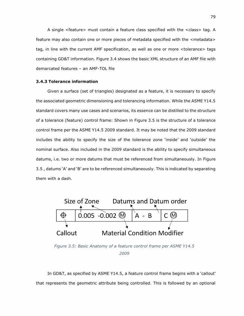
79

A single <feature> must contain a feature class specified with the <class> tag. A

feature may also contain one or more pieces of metadata specified with the <metadata>

tag, in line with the current AMF specification, as well as one or more <tolerance> tags

containing GD&T information. Figure 3.4 shows the basic XML structure of an AMF file with

demarcated features – an AMF-TOL file

3.4.3 Tolerance information

Given a surface (set of triangles) designated as a feature, it is necessary to specify

the associated geometric dimensioning and tolerancing information. While the ASME Y14.5

standard covers many use cases and scenarios, its essence can be distilled to the structure

of a tolerance (feature) control frame: Shown in Figure 3.5 is the structure of a tolerance

control frame per the ASME Y14.5 2009 standard. It may be noted that the 2009 standard

includes the ability to specify the size of the tolerance zone ‘inside’ and ‘outside’ the

nominal surface. Also included in the 2009 standard is the ability to specify simultaneous

datums, i.e. two or more datums that must be referenced from simultaneously. In Figure

3.5 , datums ‘A’ and ‘B’ are to be referenced simultaneously. This is indicated by separating

them with a dash.

In GD&T, as specified by ASME Y14.5, a feature control frame begins with a ‘callout’

that represents the geometric attribute being controlled. This is followed by an optional

Figure 3.5: Basic Anatomy of a feature control frame per ASME Y14.5

2009

80

specification of the specific form of that attribute, for example spherical versus cylindrical

diameter, and the size of the tolerance zone that the as–produced part surfaces must fall

within. The tolerance zone may be bidirectional, with the same deviation allowed both

inward and outward from the nominal surface, or with specific allowable deviations

depending on the side. The size of the zone may be augmented with a material condition

modifier – Maximum Material Condition (MMC), Least Material Condition (LMC), and

Regardless of Feature Size (RFS). If no material condition modifier is present, RFS is

implied. A material condition modifier modifies the allowable size of the tolerance zone

based on the as-produced size of the feature. A feature control frame that specifies a

tolerance of orientation or position must include one or more datums. In ASME Y 14.5, a

datum is specified by a capital letter, ‘A’ onward, that is attached to a feature, the datum

feature. Datum may themselves be toleranced with respect to other (datums) features,

creating a ‘tolerance chain’.

Tolerances of form and pose (position and orientation) in AMF-TOL are added to

features by means of the <tolerance> tag. Each <tolerance> tag captures a single feature

control frame. A tolerance element must contain a “callout" attribute. The required callout

attribute holds a string describing the tolerance callout. Examples include orientation,

cylindricity, and planarity. It is the responsibility of the user / software generating an AMF-

TOL file to ensure the callout is compatible with the feature class. In order to convey

information not necessarily covered by the ASME Y 14.5 system, tolerances of size such

as ‘diameter’ and surface quality such as ‘Ra’ may also be used as callouts.

The size of the tolerance zone is specified by means of a required <maximum> and

optional <minimum> tag, each holding a single floating point value. If minimum is not

present, the value present in the <maximum> tag is interpreted as the size of the

bidirectional tolerance zone. If both <maximum> and <minimum> are present, the value

in <maximum> represents the portion of the tolerance zone outside the nominal surface

81

and the value in <minimum> represents the portion of the tolerance zone inside the

nominal surface. This approach deviates from ASME Y14.5 2009 but is equivalent and

more in line with industry practice. When the tolerance callout represents size, maximum

and minimum are interpreted as limits on the size directly. As with callout, it is up to the

user/software system creating an AMF-TOL file to ensure that maximum and minimum

values have logical meaning. For example, a minimum value is not generally applicable

for flatness or cylindricity callouts.

If a material condition modifier is specified for the tolerance, it is provided by means

of a “condition” attribute in the <tolerance> element. As with ASME Y14.5, the omission

of the material condition implies regardless of feature size (RFS).

Datums are specified within a tolerance by means of one or more <datum> tags.

Each datum must contain an “id” attribute, which holds the AMF-TOL feature id of the

Figure 3.6: Interpretation of tolerance zone from <maximum> and

<minimum> tags. Top showing interpretation if both tags are

present, bottom showing interpretation if <minimum> is omitted

82

datum feature. Unlike ASME Y 14.5 datums are specified by simply providing their ID and

not with a capital letter. If a letter designating a datum is required, it may be provided in

metadata in the datum feature. Apart from the datum ID a <datum> element may also

contain optional “condition” and “primacy” attributes. The “condition” attribute, specifies

the material condition off the datum feature at which the tolerance applies, as specified

by ASME Y 14.5. The “primacy” attribute holds a Boolean true / false value to specify

whether the datum is primary, secondary or tertiary in the following manner:

Datums are always interpreted in the order in which they are specified in the

<tolerance> element.

If a datum contains a “primacy” value of true, its order with respect to the other

datums is considered fixed. A missing “primacy” attribute is considered equivalent

to a “primacy” of false.

Figure 3.7: Cylinder feature showing callout examples

83

3.4.4 Nominal size

It should be noted that the AMF-TOL scheme does not include a specification for

nominal dimensions or other parameters of size or position. These dimensions must be

extracted directly from the underlying tessellated geometry. This design choice was made

in order to prevent potential conflicts between specified size parameters and the actual

geometry of the part. This forces systems which require nominal size information to

expend additional effort. However, since algorithms for performing these computations

are prevalent in the literature, omitting nominal size information in AMF-TOL was

considered an acceptable tradeoff.

84

3.4.5 Elements added to the AMF Specification

Table 3.1 contains a list of XML tags and attributes added to the AMF Standard

specification. This table is an extension to Table A 1.1 AMF Elements of the AMF Standard

specification. Figure 3.8 shows these extensions in a UML format

Table 3.1: AMF-TOL Elements.

Element Parent

Element(s)

Attributes Multi

Elements?

Description

<features> <object> No Container for all

features

<feature> <features> id

(integer)

Yes Container for all

information pertaining

to a single feature

<featureid> <triangle> No id of the feature the

triangle is associated

with

<class> <feature> No Class of the feature

<tolerance> <feature> Callout

condition

Yes A tolerance frame of

the feature

<datum> <tolerance Featureid

condition

primacy

Yes A datum for the

tolerance callout

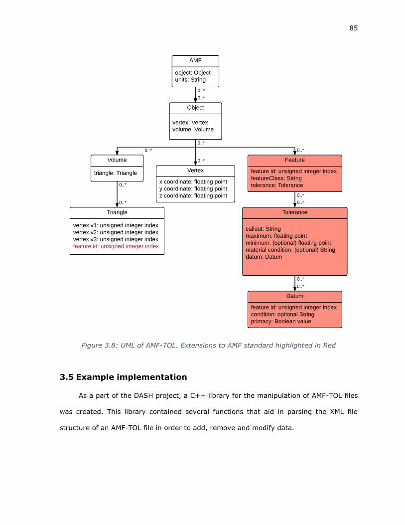
85

3.5 Example implementation

As a part of the DASH project, a C++ library for the manipulation of AMF-TOL files

was created. This library contained several functions that aid in parsing the XML file

structure of an AMF-TOL file in order to add, remove and modify data.

Figure 3.8: UML of AMF-TOL. Extensions to AMF standard highlighted in Red

86

The C++ library was used as a basis of the ‘AMFCreator’ software package Figure

3.9. This software package provides a graphic user interface in which a user may import

tessellated geometry into an AMF file, mark triangles, and associated them with features.

The software also allows for GD&T and the information to be added to these features.

3.6 Observations

The approach presented here, the AMF-TOL specification, has several attributes and

trade-offs. Most importantly, this approach imposes very few requirements on any

software dealing with either of the AMF-TOL scheme or with the base AMF specification.

The software need not track nominal geometry size, enforce part orientation (all

tolerances are with respect to other features and not with respect to any global coordinate

system) or the order of volumes and the triangles contained therein. In fact, software

schemes completely unaware of the AMF-TOL approach may load and modify files without

Figure 3.9: AMF Creator software showing ability to manipulate AMF-TOL files

87

impacting AMF-TOL specific data, if these systems preserve unrecognized structures in

the XML document.

Composability and reusability, as identified in the synthesis of requirements, is

enabled by the simplified and extensible XML structure, by the minimal requirements

imposed by this extension, and by the presence of a scheme for adding arbitrary quantities

of metadata upon which a suitable ontology may act to encode pertinent information.

Of particular interest is the suitability of the AMF-TOL format for finite element

analysis and topology optimization systems since such systems require tessellated

geometry as input. Currently, in order to utilize such systems as a part of the AM/Hybrid

process planning chain, information on functional surfaces as well as operating conditions

must be manually input. Since AMF-TOL includes information on features and tolerances

along with metadata that may hold application notes in a structured manner, it may serve

as a possible basis for the automated application of these advanced techniques as a part

of a process planning system. This would enable the analysis and modification of the part

geometry for maximal performance and minimal cost based on the specific system

selected for its manufacture, while still preserving the design intent as encapsulated in

AMF-TOL.

One primary deficiency in utilizing AMF as a geometric model format is the inexact

nature of tessellated geometry. While this is mitigated to a large extent by the inclusion

of curved triangles in AMF, exact geometry as present in solid modeling formats will always

be more precise. However, since the object of the manufacturing system used to produce

parts to within a tolerance specification, it is likely sufficient for the vast majority of

conceivable applications to simply provide a tessellated geometry representation that is

sufficiently precise.

88

3.6.1 Future developments

3.6.1.1 Ontology:

The AMF-TOL extension defines an XML structure for demarcating features and

structuring tolerances (feature control frame) in a format that is simple to process and

read by both users and software. However, for correct processing across a variety of

software systems, an ontology of terms for defining feature classes, tolerance callouts and

other strings, must be developed. Such an ontology must also include a basis for defining

new terms as required by varied processing systems in order to accommodate needs that

have not yet been anticipated. These terms must not conflict with existing terminology

and structured information.

A wide variety of tolerance and feature ontologies are available to draw from in the

literature [31]–[35]. Perhaps the best strategy would be to adopt a scheme from an allied

standard such as QIF, thereby improving compatibility and minimizing the need for

translation between schemes when applications intersect.

3.6.1.2 Standardized parameter extraction:

As indicated, the AMF-TOL scheme does not include nominal dimensions of features.

In order for many types of processing, for example subtractive finish machining, the

nominal feature dimensions must be extracted from the geometry. If different applications

use different approaches for performing this operation, given the inexact nature of

tessellated geometry, different results may be obtained leading to conflicts and potential

errors. To mitigate this, a future development might include a standard specification for a

parameter extraction algorithm based on, for example principal component analysis and

gauging principles. This is similar to the existing AMF standard specifying an algorithm for

the subdivision of curved triangles.

89

3.6.1.3 Compliance with ASME Y 14.5

The current form of the tolerance specification in AMF-TOL covers a majority of cases

encountered in common practice. However, several important aspects of ASME Y 14.5

cannot be addressed with the current scheme.

Projected tolerance zones: projected tolerance zones are a method used to

specify tolerances when the geometry of the feature must control the extents of a

mating structure, away from the geometry off the feature itself. The most common

example is a hole constraining the location of a pin that must fit within a corresponding

hole in a mating part. Specification of projected tolerance zones requires an

unambiguous specification of the direction ‘away’ from the feature geometry in which

the projected tolerance applies. An unambiguous way of representing this has not yet

been developed. Such a strategy may be developed as a part of the standardized

extraction procedure for nominal part geometry. Upon the development of such a

system a projected tolerance zone specification may be developed.

Meta features: 'meta-features’ are features associated with geometry not directly

associated with surfaces, but as a mathematical abstraction of the relationship of

multiple surfaces. Examples include a line formed by the intersection of two planes, a

point formed by the intersection of a cylinder axis and the plane or a midplane defined

by two parallel regions. A specification that can represent meta-features and

associated tolerances will help capture a wider variety of cases encountered in industry

practice.

Compound features: compound features are features that consist of multiple

distinct basic feature types. For example, a slot consists of three surfaces – two walls

and a base (the wall may be planes or surfaces). For completeness and compliance

with industry practice, a scheme for representing a feature composed of multiple

existing features is required. Much of these requirements can be met by demarcating

90

each of the components of a compound feature separately and applying appropriate

tolerances between them. However, this is cumbersome and a true compound feature

definition schema would greatly simplify these use cases.

3.6.1.4 Compliance with other emerging standards

While ASME Y 14.5 style tolerances cover the vast majority of uses required in

manufacturing industrial parts, this standard is largely geared towards prismatic,

orthogonal geometries. To address the more organic geometries that AM systems are

increasingly being required to produce, the ASME F 42 committee is developing ASME Y

14.46 approach for tolerancing geometries. A future version of AMF-TOL may include

tolerances as specified by the standard and also those specified by other emerging

schemes such as step AP 242 and the QIF standard.

3.7 Conclusions

This chapter presented an analysis of the deficiencies plaguing modern

manufacturing, specifically in the representation of geometry for process planning in

additive and hybrid manufacturing contexts. By analyzing requirements as extracted from

a review of the literature and recognizing the advantages proposed by utilizing existing

standards, an extension to the AMF file format that includes features and tolerances has

been developed and presented. This format contains the required basis for greatly

simplified transference of information between the stages of a manufacturing system that

requires varied process planning strategies.

In the context of the DASH process, the AMF stall scheme contains all information

required for the selection of critical surfaces, for addition of machining allowances and

subsequent localization and finish machining. This satisfies at least one instance in which

the utility of this scheme is proven. It is hoped that wider adoption of this scheme or

development thereof will create opportunities for a wide variety of intelligent process

91

planning and analysis systems to interact correctly and in a simplified manner and thereby

deliver greater value.

92




[2] J. Hiller and H. Lipson, “STL 2.0: a proposal for a universal multi-material Additive

Manufacturing File format,” in Proc. Solid Freeform Fabrication Symposium (SFF’09),

Austin, Texas, 2009, pp. 266–278.

[3] B. Starly, A. Lau, W. Sun, W. Lau, and T. Bradbury, “Direct slicing of STEP based

NURBS models for layered manufacturing,” Comput.-Aided Des., vol. 37, no. 4, pp.

387–397, Apr. 2005.

[4] ASTM, “Additive Manufacturing File Format (AMF) 1.1,” ISO/ASTM 52915:2013.

[5] “ASME Y14.5 - Dimensioning and Tolerancing.” [Online]. Available:

https://www.asme.org/products/codes-standards/y145-2009-dimensioning-and-

tolerancing. [Accessed: 22-Mar-2016].

[6] “ASME Y14.41 - Digital Product Definition Data Practices.” [Online]. Available:

https://www.asme.org/products/codes-standards/y1441-2012-digital-product-

definition-data. [Accessed: 22-Mar-2016].

[7] “Committee F42 on Additive Manufacturing Technologies.” [Online]. Available:

http://www.astm.org/COMMITTEE/F42.htm. [Accessed: 15-Apr-2016].

[8] D. B. Kim, P. Witherell, R. Lipman, and S. C. Feng, “Streamlining the additive

manufacturing digital spectrum: A systems approach,” Addit. Manuf., vol. 5, pp. 20–

30, Jan. 2015.

[9] F. Ahmed and S. Han, “Semantic Mismatches for Interoperability of Product and

Manufacturing Information,” Int. J. CADCAM, vol. 13, no. 2, Jul. 2013.

[10] F. Ahmed and S. Han, “Interoperability of product and manufacturing information

using ontology,” Concurr. Eng., vol. 23, no. 3, pp. 265–278, Sep. 2015.

[11] M. D. Monzón, Z. Ortega, A. Martínez, and F. Ortega, “Standardization in additive

manufacturing: activities carried out by international organizations and projects,” Int.

J. Adv. Manuf. Technol., pp. 1–11, Sep. 2014.

[12] K. Jurrens, “NIST measurement science for additive manufacturing,” in National

Institute for Standards in Technology. Presentation for PDES, Inc., workshop, 2013.

93

[13] Y. Lu, S. Choi, and P. Witherell, “Towards an Integrated Data Schema Design for

Additive Manufacturing: Conceptual Modeling,” in ASME 2015 International Design

Engineering Technical Conferences and Computers and Information in Engineering

Conference, 2015, pp. V01AT02A032–V01AT02A032.

[14] “3MF | 3MF Specification.” .

[15] N. US Department of Commerce, “Digital Thread for Smart Manufacturing.” [Online].

Available: http://www.nist.gov/el/msid/syseng/dtsm.cfm. [Accessed: 20-Mar-

2016].

[16] W. Cheng, J. y. h. Fuh, A. y. c. Nee, Y. s. Wong, H. t. Loh, and T. Miyazawa, “Multi‐objective optimization of part‐ building orientation in stereolithography,” Rapid

Prototyp. J., vol. 1, no. 4, pp. 12–23, Dec. 1995.

[17] C. M. Lynn, A. West, and D. W. Rosen, “A process planning method and data format

for achieving tolerances in stereolithography,” in Proceedings from the 1998 Solid

Freeform Fabrication Symposium, Austin, TX, 1998.

[18] C. Lynn‐Charney and D. W. Rosen, “Usage of accuracy models in stereolithography

process planning,” Rapid Prototyp. J., vol. 6, no. 2, pp. 77–87, Jun. 2000.

[19] R. Paul and S. Anand, “Optimization of layered manufacturing process for reducing

form errors with minimal support structures,” J. Manuf. Syst., 2014.

[20] “ISO 10303-203:2011 - Industrial automation systems and integration -- Product

data representation and exchange -- Part 203: Application protocol: Configuration

controlled 3D design of mechanical parts and assemblies.” [Online]. Available:

http://www.iso.org/iso/iso_catalogue/catalogue_tc/catalogue_detail.htm?csnumber

=44305. [Accessed: 18-Mar-2016].


data representation and exchange -- Part 214: Application protocol: Core data for

automotive mechanical design processes.” [Online]. Available:

http://www.iso.org/iso/iso_catalogue/catalogue_ics/catalogue_detail_ics.htm?csnu

mber=43669. [Accessed: 18-Mar-2016].


data representation and exchange -- Part 238: Application protocol: Application

interpreted model for computerized numerical controllers.” [Online]. Available:

http://www.iso.org/iso/iso_catalogue/catalogue_tc/catalogue_detail.htm?csnumber

=38036. [Accessed: 20-Mar-2016].

94


data representation and exchange -- Part 242: Application protocol: Managed model-

based 3D engineering.” [Online]. Available:

http://www.iso.org/iso/home/store/catalogue_ics/catalogue_detail_ics.htm?csnum

ber=57620. [Accessed: 18-Mar-2016].

[24] A. B. Feeney, S. P. Frechette, and V. Srinivasan, “A portrait of an ISO STEP

tolerancing standard as an enabler of smart manufacturing systems,” J. Comput. Inf.

Sci. Eng., vol. 15, no. 2, p. 021001, 2015.

[25] R. Paul and S. Anand, “A new Steiner patch based file format for Additive

Manufacturing processes,” Comput.-Aided Des., vol. 63, pp. 86–100, Jun. 2015.

[26] Y. F. Zhao, J. A. Horst, T. R. Kramer, W. Rippey, and R. Brown, “Quality Information

Framework–Integrating Metrology Processes,” in Information Control Problems in

Manufacturing, 2012, vol. 14, pp. 1301–1308.

[27] X. Zhao, T. M. Kethara Pasupathy, and R. G. Wilhelm, “Modeling and representation

of geometric tolerances information in integrated measurement processes,” Comput.

Ind., vol. 57, no. 4, pp. 319–330, May 2006.

[28] A. R. Nassar and E. W. Reutzel, “A proposed digital thread for additive

manufacturing,” in International Solid Freeform Fabrication Symposium, Austin,

Texas.[Online]. http://utwired. engr. utexas. edu/lff/symposium/proceedingsarchiv

e/pubs/Manuscripts/2013/2013-02-Nassar. pdf [Accessed: 10-Feb-2015], 2013.

[29] Y. S. Hong and T. C. Chang, “A comprehensive review of tolerancing research,” Int.

J. Prod. Res., vol. 40, no. 11, pp. 2425–2459, Jan. 2002.

[30] N. Anwer, B. Schleich, L. Mathieu, and S. Wartzack, “From solid modelling to skin

model shapes: Shifting paradigms in computer-aided tolerancing,” CIRP Ann. -

Manuf. Technol., vol. 63, no. 1, pp. 137–140, 2014.

[31] J. Wang, L. Zhang, L. Duan, and R. X. Gao, “A new paradigm of cloud-based

predictive maintenance for intelligent manufacturing,” J. Intell. Manuf., pp. 1–13,

Mar. 2015.

[32] D. Wu, D. W. Rosen, L. Wang, and D. Schaefer, “Cloud-based design and

manufacturing: A new paradigm in digital manufacturing and design innovation,”

Comput.-Aided Des., vol. 59, pp. 1–14, Feb. 2015.

95

[33] L. Zhang, Y. Luo, F. Tao, B. H. Li, L. Ren, X. Zhang, H. Guo, Y. Cheng, A. Hu, and Y.

Liu, “Cloud manufacturing: a new manufacturing paradigm,” Enterp. Inf. Syst., vol.

8, no. 2, pp. 167–187, Mar. 2014.

[34] R. T. Chaparala, N. W. Hartman, and J. Springer, “Examining CAD Interoperability

through the Use of Ontologies,” Comput.-Aided Des. Appl., vol. 10, no. 1, pp. 83–

96, Jan. 2013.

[35] H. Panetto, M. Dassisti, and A. Tursi, “ONTO-PDM: Product-driven ONTOlogy for

Product Data Management interoperability within manufacturing process

environment,” Adv. Eng. Inform., vol. 26, no. 2, pp. 334–348, Apr. 2012.

96

Chapter 4

AUTOMATIC MESH OFFSET FOR THE GENERATION OF

MACHINING ALLOWANCES

Finish machining is a process by which material is removed from a near-net shape

workpiece by means of a CNC machine tool, in order to obtain the specified final part

geometry to the required surface accuracy and tolerances. For this to be successfully

achieved, the initial part must have additional material present over all surfaces that are

to be subtractively processed, to account for defects in the near-net production process,

as well as to account for the requirements of the subtractive methodology. In order to

achieve this requirement, prior to production in the near-net system, the nominal part

geometry on all surfaces to be finished is ‘overgrown’, i.e. offset in the direction ‘outside’

the geometry.

The purpose of this chapter is to present a methodology for the addition of machining

allowances to an AMF-TOL file, following the scheme presented in Chapter 3. The following

sections provide a background and motivation, followed by a literature review on the

automatic addition of machining allowances, and mesh deformation. A methodology for

offsetting vertices and generating machining allowance ‘volumes’ is then presented,

followed by an analysis of the scheme and conclusions.

4.1 Background and Motivation

In current manufacturing practice many parts are created by processes in which a

near net shape process is used to create an approximate geometry followed by a

subtractive process that generates final surfaces with the required dimensions and

tolerances. Examples include casting and forging processes followed by finish machining.

97

In many cases, only the functional regions of a cast or forged part are finished machined.

The remainder of the part surfaces are left unfinished.

In order to successfully finish machine a part, sufficient excess material must be

present over all required feature surfaces. A workpiece that meets this requirement is

sometimes referred to as ‘steel safe’. This requirement for excess material is modeled by

backward planning from the final model, which represents the design intent, and

generating a series of models representing the target of each stage of manufacturing.

Each target model accounts for the requirements (machining allowances) for each the

subsequent downstream process. This step is performed manually in a CAD package,

based on the experience of the process planner together with any standards and best

practices established by the specific industry.

In this approach, machining allowances are not added to a model so much as models

are created accounting for any allowances required by downstream processes. This

process is time consuming and slow, and contributes to high costs and time-to-market.

When required part quantities are low, these effects are quite pronounced.

In order to aid this, several automated process planning systems for casting and

forging have been developed. For example, In [1], Kulon et al. present a knowledge-based

model for the generation of a process plan for forging. In this work machining allowances

are a simple surface offset applied to the entire solid geometry model. A specific algorithm

for the surface offset is not presented, with the implication that it may be generated using

the underlying geometry kernel of a solid modeling package. The BS 4114 standard is

used as a basis for deciding exact quantity of surface offset/machining allowance. Caporalli

et al. [2] present an expert planning system for flashless forging in which machining

allowances are designated to be added to surfaces that require finish machining. However,

the actual part modification is not performed automatically, instead requiring a user to

perform this step manually in CAD software, following the directions of the expert system.

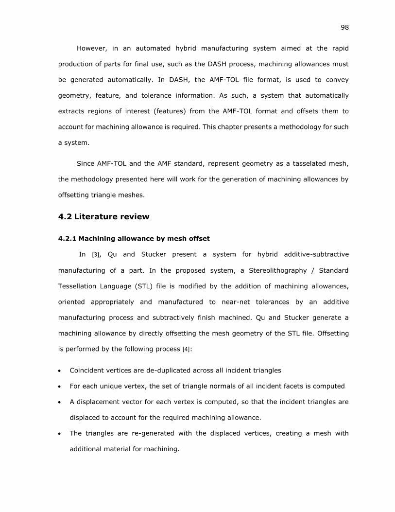
98

However, in an automated hybrid manufacturing system aimed at the rapid

production of parts for final use, such as the DASH process, machining allowances must

be generated automatically. In DASH, the AMF-TOL file format, is used to convey

geometry, feature, and tolerance information. As such, a system that automatically

extracts regions of interest (features) from the AMF-TOL format and offsets them to

account for machining allowance is required. This chapter presents a methodology for such

a system.

Since AMF-TOL and the AMF standard, represent geometry as a tasselated mesh,

the methodology presented here will work for the generation of machining allowances by

offsetting triangle meshes.

4.2 Literature review

4.2.1 Machining allowance by mesh offset

In [3], Qu and Stucker present a system for hybrid additive-subtractive

manufacturing of a part. In the proposed system, a Stereolithography / Standard

Tessellation Language (STL) file is modified by the addition of machining allowances,

oriented appropriately and manufactured to near-net tolerances by an additive

manufacturing process and subtractively finish machined. Qu and Stucker generate a

machining allowance by directly offsetting the mesh geometry of the STL file. Offsetting

is performed by the following process [4]:

Coincident vertices are de-duplicated across all incident triangles

For each unique vertex, the set of triangle normals of all incident facets is computed

A displacement vector for each vertex is computed, so that the incident triangles are

displaced to account for the required machining allowance.

The triangles are re-generated with the displaced vertices, creating a mesh with

additional material for machining.

99

Figure 4.1 shows the approach taken By Qu and Stucker [3], [4] in generating vertex

displacement vectors for generation of machining allowances. The displacement vector is

generated such that it projects onto all incident normal vectors, which have been scaled

to match the required machining allowance, as shown in Figure 4.2. If the number of

indecent triangles is exactly three, this displacement vector can be solved for directly, as

seen in Equation ( 1 ).

( 1 )

In Equation ( 1 ), on the LHS, [i j k]’ 1 through 3 represent the indecent triangle

normals and [id jd kd]’ is the desired displacement vector. On the RHS, ‘A’ is the desired

allowance. The displacement vector may be solved for directly.

Figure 4.1: Projection of displacement vector onto incident

triangle normals

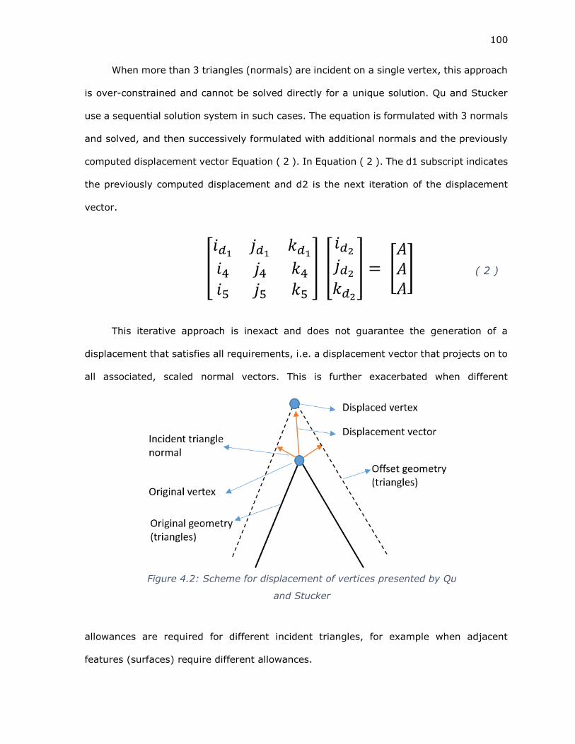
100

When more than 3 triangles (normals) are incident on a single vertex, this approach

is over-constrained and cannot be solved directly for a unique solution. Qu and Stucker

use a sequential solution system in such cases. The equation is formulated with 3 normals

and solved, and then successively formulated with additional normals and the previously

computed displacement vector Equation ( 2 ). In Equation ( 2 ). The d1 subscript indicates

the previously computed displacement and d2 is the next iteration of the displacement

vector.

( 2 )

This iterative approach is inexact and does not guarantee the generation of a

displacement that satisfies all requirements, i.e. a displacement vector that projects on to

all associated, scaled normal vectors. This is further exacerbated when different

allowances are required for different incident triangles, for example when adjacent

features (surfaces) require different allowances.

Figure 4.2: Scheme for displacement of vertices presented by Qu

and Stucker

101

This deficiency necessitates the creation of an improved algorithm for the generation

of the displacement vector, that can better account for the needs imposed by the presence

of multiple incident triangles each requiring different machining allowances. Several other

schemes that address this challenge have been presented in the literature.

Kim et al. [5] present a scheme for offsetting meshes by the multiple normal vectors

of a vertex. In this scheme an iterative averaging scheme is presented for the computation

of a displacement vector for incident triangle normals that are well aligned. Alignment is

measured by testing the magnitude of vector cross products against a threshold. For

normal vectors that are not well aligned, the vertex is duplicated and displaced in multiple

directions and the resulting gap is filled with a blend surface. Similar to the approach

presented by Qu and Stucker [4], this method is inexact.

Chen et al. [6], identifying the potential for mesh errors vertex displacement

schemes that are applied with large offset numbers, present a point based mesh offset

scheme. In this scheme, offsets are generated by sampling the mesh, offsetting the

sampled points and generating a new offset by re-meshing the offset points by means of

an iso-surface. This approach has the potential to be slow and requires the use of mesh-

reduction algorithms to reduce the numbers of triangles.

Finally, modern editions of Materialise Magics ™ mesh processing software have a

tool for generating ‘Milling offsets’ on selected part surfaces.

4.2.2 Other approaches to machining allowance in Hybrid systems

Several authors have presented hybrid manufacturing systems in which a deposition

based AM system such as Directed Energy Deposition (DED) or Fused Deposition Modelling

(FDM) AM system is integrated into a CNC system already capable of subtractive

processing. The AM system is used to additively generate near-net-shape geometries,

either completely afresh or starting with a pre-existing part that requires rework, followed

102

by subtractive finishing by the CNC system. Such systems also require the addition of a

machining allowance prior to the deposition of material.

The Arc-HLM (Hybrid Layer Manufacturing) system presented by Karunakaran et al.

[7] a Gas Metal Arc Welding (GMAW, also known as Metal Inert-Gas, MIG) welding system

is mounted in parallel to a CNC milling head. The GMAW system is used to rapidly deposit

material and the CNC machine is used to both smooth layers during manufacture as well

as to finish machine all part surfaces after deposition is completed. In this system,

allowances are added at the slicing and tool-path generation level, as a distance beyond

the slice boundary to which the tool-paths for weld deposition are generated [8].

While these approaches may prove successful in their respective domains, their

utility in a Hybrid process in which existing AM and SM systems are tied together with

software, such as DASH, is limited due to the lack of direct control over slicing and tool-

paths.

4.3 Problem description

A part model represented in the AMF-TOL format contains several features, each

consisting of multiple demarcated triangles. In order to add a machining allowance,

surfaces must be generated parallel to and at an offset from each feature surface, at a

Figure 4.3: Offset with multiple features

103

displacement equal to the required machining allowance. Additionally, the regions

bordering multiple features must be offset appropriately accounting for the different

required machining allowances. This is illustrated in Figure 4.3. In addition, the edges of

the offset surfaces must be ‘stitched’ back to the original model, in order to create a closed

surface, suitable for processing by AM software systems, as seen in Figure 4.4.

4.4 Methodology

From the literature review and given the requirements of adding machining

allowances to parts represented in the AMF-TOL file format, the approach selected is the

generation of an offset by the displacement of vertices. Displacing vertices changes the

geometry of the incident triangles while keeping their topology intact.

The AMF file format (and AMF-TOL) supports the concept of volumes – closed

manifold surfaces each representing a distinct section of the part. Instead of directly

modifying the underlying part geometry, we generate a volume representing the

Figure 4.4: Stitching edges together to form a closed volume

104

machining allowance that sits directly coincident with the features of interest. In this way

a combined (Boolean union) volume may be exported for printing while still preserving

the original geometry for further processing, if necessary. This approach is illustrated in

Figure 4.5.

The following procedure is used to generate a volume representing the machining

allowance:

1. Extract the set of triangles that require a machining allowance.

2. Compute the normal vectors of the triangles as specified by the AMF standard.

a. Scale the magnitude normals to match the required allowance.

3. Extract the set of vertices referred to by the set of feature triangles and associate

each vertex with the scaled normals (from step #2) of each incident triangle

4. Compute a displacement vector for each vertex such that all incident triangles are

offset by the required allowance. The procedure for this displacement computation

is detailed in Section 4.4.1

5. Duplicate each vertex and offset the duplicates by the associated, computed,

displacement.

6. Generate triangles to form the machining allowance

a. Duplicate the set of feature triangles and replace each vertex with the

corresponding displaced vertex. This effectively displaces each triangle by

the required machining allowance.

b. Duplicate the set of feature triangles again and reverse their direction by

reordering their vertices.

c. Detect the open edges of the two sets of triangles – displaced and reversed

(from steps 6.a and 6.b) and generate triangles together that stitch the

edges together. This procedure is discussed in section 4.4.2

105

7. Create a new volume in the AMF object, to represent the machining allowance, and

add the triangles from 6a through c to it.

4.4.1 Procedure for computing vertex displacement vector

As indicated in Figure 4.1, the displacement vector must project onto all incident

triangle normals, each scaled by the required machining allowance. When different

allowances are required for each feature, this may be formulated as in Equation ( 3 ). In

Equation ( 3 ), �⃗⃗� is the desired vertex displacement vector, A1 through Ak and 𝑁1⃗⃗ ⃗⃗ through

𝑁𝑚⃗⃗⃗⃗⃗⃗ are, respectively, the desired machining allowances and normals of all incident

triangles

Each equation in Equation ( 3 ) mathematically states the displacement vector

must project exactly onto all incident triangle normals.

Figure 4.5: Machining allowance as a volume in the AMF object. (a) shows an AMF

file with a feature highlighted, (b) shows the machining allowance as a closed

volume, and (c) depicts the machining allowance together with the original file

106

( 3 )

The formulation in Equation ( 3 ) is in general unsolvable when there are more than

three incident triangle normals, requiring iterative solution schemes as in Qu and Stucker

[4]. However, it may be reformulated as a minimization problem, as in Equation ( 4 ). The

length of the Displacement vector is minimized while ensuring that the projection onto

each, scaled, incident normal is greater than 0. In other words, Equation ( 4 ) states ‘find

the smallest displacement vector such that each incident triangle has at least the

required allowance’. In the limiting case, this problem reduces to the exact projection

from Equation ( 3 ).

With this reformulation, the computation of the vertex displacement vector takes

the following form:

1. Extract the set of vertices to be offset

2. Associate each vertex with the set of incident triangle normals, each scaled

to the required allowance

3. Construct a non-linear optimization (minimization) system in three variables

iD, jD and kD, the components of the displacement vector �⃗⃗� s.t.

a. Minimizing || [iD, jD and kD] ||

b. Subject to (𝑖𝐷𝑖𝑛𝑁𝐴𝑛 + 𝑗𝐷𝑗𝑛

𝑁𝐴𝑛 + 𝑘𝐷𝑘𝑛𝑁𝐴𝑛) ≥ 0 for each incident normal

where 𝑖𝑛𝑁 is the ‘i’ component of the nth incident triangle normal and

𝐴𝑛 is the associated required allowance (magnitude)

4. Solve for �⃗⃗� . This is the required displacement vector for the vertex

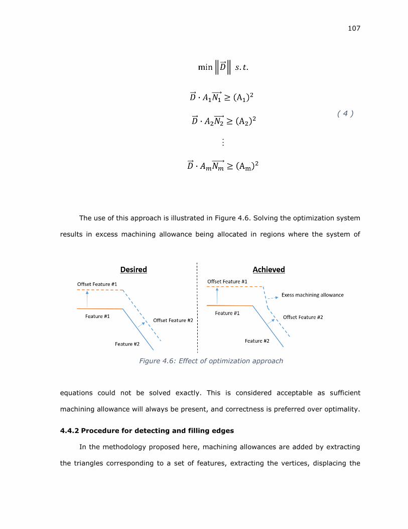
107

( 4 )

The use of this approach is illustrated in Figure 4.6. Solving the optimization system

results in excess machining allowance being allocated in regions where the system of

equations could not be solved exactly. This is considered acceptable as sufficient

machining allowance will always be present, and correctness is preferred over optimality.

4.4.2 Procedure for detecting and filling edges

In the methodology proposed here, machining allowances are added by extracting

the triangles corresponding to a set of features, extracting the vertices, displacing the

Figure 4.6: Effect of optimization approach

108

vertices and re-creating the triangles with these displaced vertices. However, the

displaced triangles will now no longer be part of a closed, manifold, volume. This included

volume must be created in order for the AMF file to be invalid. The opposite face of the

required volume can be created in duplicating the original triangles again, and reversing

their direction. This leaves the task of closing the open edges between the displaced and

the reversed triangles.

The first step is detecting the open edges. We use the observation that any given

pair of vertices is shared by two triangles. This is analogous to a ‘half-edge’ data structure

common in many computational geometry applications. Any edge, i.e. pair of vertices that

is present in only one triangle denotes an open edge. The following steps can therefore

be used to extract a set of open edges:

1. Assign unique IDs to each triangle in the original set of feature triangles. If stored

in an array, array indices are sufficient.

2. Construct a data structure which associates the vertex index with the unique IDs

of each triangle that refers to that vertex.

3. For each triangle, for each pair of vertices, use the data structure from step #2

to search for the set of triangles that referred to both vertices. i.e.

a. Given the vertices of a triangle 𝑉𝑎 , 𝑉𝑏 , 𝑉𝑐 with pairs [𝑉𝑎𝑉𝑏] ; [𝑉𝑏𝑉𝑐] ; [𝑉𝑐𝑉𝑎]

b. Extract the sets of triangles 𝑇𝑎 , 𝑇𝑏 , 𝑎𝑛𝑑 𝑇𝑐 that contain 𝑉𝑎 , 𝑉𝑏 𝑎𝑛𝑑 𝑉𝑐

respectively

c. Compute set intersections 𝑇𝑎 ∩ 𝑇𝑏 , 𝑇𝑏 ∩ 𝑇𝑐 𝑎𝑛𝑑 𝑇𝑐 ∩ 𝑇𝑎

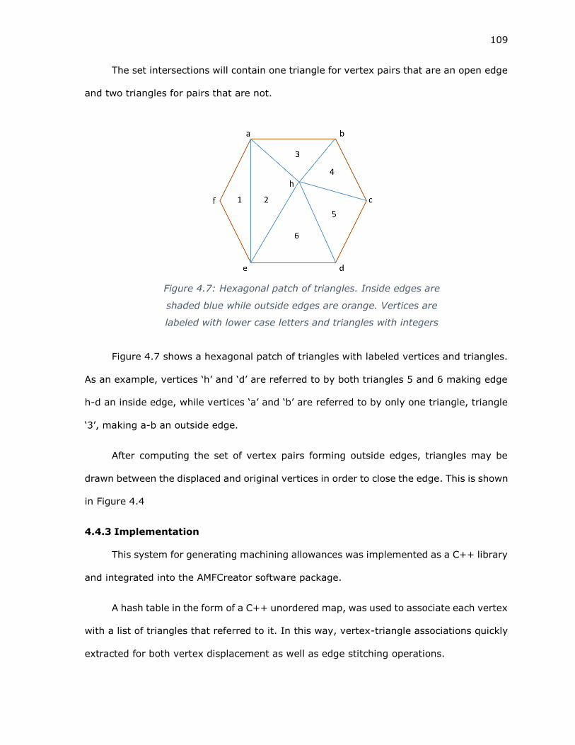
109

The set intersections will contain one triangle for vertex pairs that are an open edge

and two triangles for pairs that are not.

Figure 4.7 shows a hexagonal patch of triangles with labeled vertices and triangles.

As an example, vertices ‘h’ and ‘d’ are referred to by both triangles 5 and 6 making edge

h-d an inside edge, while vertices ‘a’ and ‘b’ are referred to by only one triangle, triangle

‘3’, making a-b an outside edge.

After computing the set of vertex pairs forming outside edges, triangles may be

drawn between the displaced and original vertices in order to close the edge. This is shown

in Figure 4.4

4.4.3 Implementation

This system for generating machining allowances was implemented as a C++ library

and integrated into the AMFCreator software package.

A hash table in the form of a C++ unordered map, was used to associate each vertex

with a list of triangles that referred to it. In this way, vertex-triangle associations quickly

extracted for both vertex displacement as well as edge stitching operations.

Figure 4.7: Hexagonal patch of triangles. Inside edges are

shaded blue while outside edges are orange. Vertices are

labeled with lower case letters and triangles with integers

110

The NLOPT library [9] was used to perform the optimization, specifically the SLSQP

(Sequential Least Squares Quadratic Programming) algorithm in this library. While a much

simpler algorithm might prove suitable for the given problem formulation, NLOPT-SLSQP

was still used in order to exploit the robustness that may be realized with a well-tested,

popular library.

Figure 4.8: Five features in an example ‘Bracket’ part. Images (a) and (e) show hole

features, while images (b), (c) and (d) show planes

Figure 4.9: Allowance added to features highlighted in Figure 4.8

111

Figure 4.8 through Figure 4.12 show the working of this system within the

AMFCreator software package. In Figure 4.8, five features in the AMF file showing a

‘Bracket’ part are shown highlighted - two cylinders and three planes. The part is

approximately 90mm long, 20mm wide and 40mm tall. Allowances of 1mm to cylinder

feature in (a), 2mm to plane feature in (b), 1mm to plane feature in (c), 5mm to plane

feature in (d) and 3mm to cylinder feature in (e) were generated. The results of this

operation are presented in Figure 4.9. The excess allowance added at the boundary of

features (c) and (d) is clearly seen.

Figure 4.10: GE Bracket part. Features are highlighted in different

colors

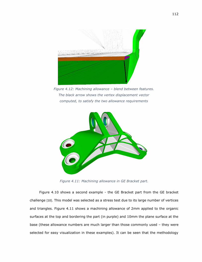
112

Figure 4.10 shows a second example - the GE Bracket part from the GE bracket

challenge [10]. This model was selected as a stress test due to its large number of vertices

and triangles. Figure 4.11 shows a machining allowance of 2mm applied to the organic

surfaces at the top and bordering the part (in purple) and 10mm the plane surface at the

base (these allowance numbers are much larger than those commonly used – they were

selected for easy visualization in these examples). It can be seen that the methodology

Figure 4.11: Machining allowance in GE Bracket part.

Figure 4.12: Machining allowance – blend between features.

The black arrow shows the vertex displacement vector

computed, to satisfy the two allowance requirements

113

presented here functions well for curved, organic surfaces as well. In Figure 4.12, a cross-

section of the machining allowance shows the relationship between the original surfaces

and the machining allowance, specifically indicating the displacement vector computed to

accommodate the two different machining allowance requirements on the two features.

4.5 Observations, future work, and conclusions

The approach for adding machining allowances presented in this chapter describes

a methodology for per-feature stock addition to a part model represented in the AMF-TOL

file format. A new vertex displacement calculation method is presented, that improves

correctness and suitability when compared to methods found in the literature.

Testing shows that this approach is sufficiently fast for use in process planning

operations. For example, the addition of machining allowances to the GE Bracket part

depicted in Figure 4.11, for example, took approximately seven seconds despite the very

large number of vertices and triangles present. This is comparable to many mesh

deformation algorithms in commercial mesh processing software packages.

The approach presented here has several weaknesses, however – handling local and

global self-intersections. Local self-intersections are caused when concave regions of a

part are offset by more than the local (concave) radius of curvature. When this happens,

the displaced triangles are often inverted and self-intersecting. A system that tracks the

topology and geometry of triangle edges before and after offsetting, and which collapses

‘bad’ edges and triangles may be able to detect and rectify this issue. Global self-

intersections are caused when the allowance added to one region of a part intersects with

another, completely separate, region. Addressing this will require a system which tracks

triangle intersections globally. In practice, this is not a major issue as machining

allowances are normally small in relation with part dimensions.

114

In addition to these challenges, several improvements may be made to the current

implementation of the algorithm. Most notably, a custom optimization solver more suitable

for this class of problem would be preferable.

In conclusion, the system presented here provides a suitable approach for the

offsetting of mesh geometries and thereby the generation of machining allowances directly

in an AMF-TOL file.

115


[1] J. Kulon, D. J. Mynors, and P. Broomhead, “A knowledge-based engineering design

tool for metal forging,” J. Mater. Process. Technol., vol. 177, no. 1–3, pp. 331–335,

Jul. 2006.

[2] Â. Caporalli, L. A. Gileno, and S. T. Button, “Expert system for hot forging design,”

J. Mater. Process. Technol., vol. 80–81, pp. 131–135, Aug. 1998.

[3] Brent Stucker and Xiuzhi Qu, “A finish machining strategy for rapid manufactured

parts and tools,” Rapid Prototyp. J., vol. 9, no. 4, pp. 194–200, Oct. 2003.

[4] Xiuzhi Qu and Brent Stucker, “A 3D surface offset method for STL‐format models,”

Rapid Prototyp. J., vol. 9, no. 3, pp. 133–141, Aug. 2003.

[5] S.-J. Kim, D.-Y. Lee, and M.-Y. Yang, “Offset Triangular Mesh Using the Multiple

Normal Vectors of a Vertex,” Comput.-Aided Des. Appl., vol. 1, no. 1–4, pp. 285–

291, Jan. 2004.

[6] Y. Chen, H. Wang, D. W. Rosen, and J. Rossignac, “A point-based offsetting method

of polygonal meshes,” ASME J. Comput. Inf. Sci. Eng. Rev., 2005.

[7] K. P. Karunakaran, S. Suryakumar, V. Pushpa, and S. Akula, “Retrofitment of a CNC

machine for hybrid layered manufacturing,” Int. J. Adv. Manuf. Technol., vol. 45, no.

7–8, pp. 690–703, Dec. 2009.

[8] S. Akula and K. P. Karunakaran, “Hybrid adaptive layer manufacturing: An Intelligent

art of direct metal rapid tooling process,” Robot. Comput.-Integr. Manuf., vol. 22,

no. 2, pp. 113–123, Apr. 2006.

[9] S. G. Johnson, The NLopt nonlinear-optimization package. 2014.

[10] “GE jet engine bracket challenge - GrabCAD.” [Online]. Available:

https://grabcad.com/challenges/ge-jet-engine-bracket-challenge/results.

[Accessed: 05-Apr-2016].

[11] J. R. Rossignac and A. A. Requicha, “Offsetting operations in solid modelling,”

Comput. Aided Geom. Des., vol. 3, no. 2, pp. 129–148, 1986.

116

Chapter 5

AUTOMATIC REGISTRATION OF SCAN DATA TO

MACHINE COORDINATE SYSTEM

3D Scanning systems produce data in the form of point clouds – sets of points

located in 3D space in the scanner’s coordinate system. In order to be useful for planning

and localization, the point data must be transformed to a coordinate system attached to

the workspace. In the context of the DASH system, toolpath planning is performed within

a CNC machine (workspace), based on a work offset (workspace coordinate system).

There are several methods that may be used to determine the transformation from

the scanner coordinate system to the workpiece coordinate system. In this chapter, a new

method of computing this transform by automatically locating and measuring datum

surfaces in scan data is presented.

5.1 Background

5.1.1 Part localization

Prior to processing in a subtractive CNC system, a workpiece must be securely

mounted and located in the CNC machine’s workspace. The activities associated with

determining the location and orientation of the workpiece in the CNC machine (workspace)

coordinate system are referred to as localization. In traditional manufacturing,

localization is performed by one of two methods – manually by a machinist or by means

of Jigs and Fixtures.

When lot size requirements are low workpieces are generally located manually - a

skilled operator uses various instruments and gauges to locate and align the datums of

the workpiece with respect to the CNC machine coordinate system, or with respect to

117

standard fixtures, such as vises and chucks already mounted and located in the machine.

This is a time consuming event and requires considerable skill and experience.

When lot size requirements are larger, Jigs and Fixtures may be used. Fixtures are

parts specifically manufactured to hold a workpiece geometry in order to present specific

workpiece surfaces to the machine tool as well as to hold the workpiece against any cutting

forces. The production of a single part may require several fixtures, each locating and

orienting the part for the production of an aspect of its final geometry. Jigs are similar to

fixtures, except that they are used to guide the tool to the part, rather than locating the

part with respect to the tool. The use of fixtures can significantly speed up the process of

mounting a part in a CNC machine – normally, the act of clamping the part in the fixture

also positions and orients it appropriately, due to the interaction between the fixture and

part geometries under clamping forces.

Jigs and Fixtures must be produced to significantly greater accuracy than the part,

often feature complicated geometry, and must themselves must be manually located in

the machine. This makes Jigs and Fixtures time consuming and expensive to produce.

Lead times of weeks to months for their production and installation are common.

Due to the relatively low accuracy of modern AM systems, especially metal AM

systems, these parts must be finish machined. However, parts manufactured by AM

systems usually feature complex geometries and small lot sizes and therefore require

considerable time to mount and locate in a CNC machine. This negates the ability of AM

systems to produce parts on-demand with short lead times. What is required is the ability

to mount a workpiece at an approximate location, measure all its surfaces, and compute

the in-machine position and orientation of the workpiece from these measurements.

118

5.1.2 Current in-machine sensing systems

The most common automated sensing system employed in a CNC machine is the

touch probe [1] [2]. In use, a touch probe is mounted in the spindle of a CNC machine,

much like a tool. The touch probe incorporates a shaft with a precision ground tip (usually

Ruby or a similar material) that is connected to a sensing and signaling apparatus. The

CNC system is used to move the probe and the sensing and signaling system signals the

CNC controller whenever the probe makes contact with the workpiece. The position of the

machine at the instant of contact is offset based on the probe’s geometry to give the

contact location on the workpiece, and recorded. Each contact of the probe tip with the

workpiece generates a single coordinate measurement on the workpiece.

In current practice, an NC program is used to guide the path taken by the probe and

to gather measurements of critical areas on the workpiece. These measurements are used

to determine the size, form, and pose (position and orientation) of the workpiece material

present.

Programming a probing routine is challenging and time consuming, even with the

aid of modern probe routing planning systems. In addition, since each touch generates a

single measurement, the measurement of an AM geometry with complicated surfaces,

which might require many thousands of samples, can be quite time consuming. Touch

probes are also limited by reach and access issues – the probe can only measure surfaces

‘visible’ to the probe/spindle and within reach of the probe shaft.

More recently scanning probes have been developed which can generate high

density measurements by continuously sampling the part surface as the probe is moved

while continuously in contact with the part. However, the challenges posed by of visibility,

access and programming time are not negated by scanning probes.

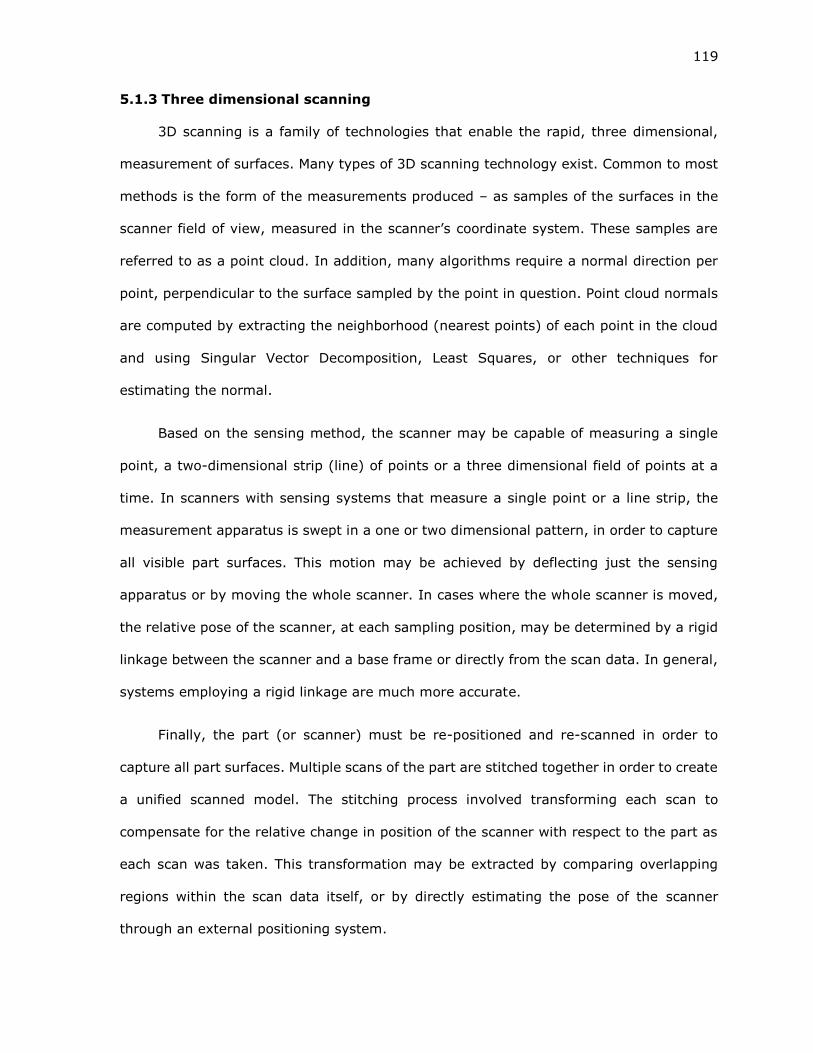
119

5.1.3 Three dimensional scanning

3D scanning is a family of technologies that enable the rapid, three dimensional,

measurement of surfaces. Many types of 3D scanning technology exist. Common to most

methods is the form of the measurements produced – as samples of the surfaces in the

scanner field of view, measured in the scanner’s coordinate system. These samples are

referred to as a point cloud. In addition, many algorithms require a normal direction per

point, perpendicular to the surface sampled by the point in question. Point cloud normals

are computed by extracting the neighborhood (nearest points) of each point in the cloud

and using Singular Vector Decomposition, Least Squares, or other techniques for

estimating the normal.

Based on the sensing method, the scanner may be capable of measuring a single

point, a two-dimensional strip (line) of points or a three dimensional field of points at a

time. In scanners with sensing systems that measure a single point or a line strip, the

measurement apparatus is swept in a one or two dimensional pattern, in order to capture

all visible part surfaces. This motion may be achieved by deflecting just the sensing

apparatus or by moving the whole scanner. In cases where the whole scanner is moved,

the relative pose of the scanner, at each sampling position, may be determined by a rigid

linkage between the scanner and a base frame or directly from the scan data. In general,

systems employing a rigid linkage are much more accurate.

Finally, the part (or scanner) must be re-positioned and re-scanned in order to

capture all part surfaces. Multiple scans of the part are stitched together in order to create

a unified scanned model. The stitching process involved transforming each scan to

compensate for the relative change in position of the scanner with respect to the part as

each scan was taken. This transformation may be extracted by comparing overlapping

regions within the scan data itself, or by directly estimating the pose of the scanner

through an external positioning system.

120

3D scanning systems possess the accuracy, flexibility and sampling density to serve

as an effective means of rapidly measuring AM parts in a CNC machine. However, since

the scan data (point cloud) is located in the scanner coordinate system, it must first be

transformed into the CNC machine coordinate system before it can be used for planning.

This transformation must account for both the relative pose of the scanner with respect

to the CNC coordinate system, as well as the translation and rotation of the CNC machine

at the time of scanning, away from the zero position. The process of transforming 3D scan

data from the base frame of the scanner to the workspace coordinate system is known as

registration.

5.2 Literature Review

5.2.1 Scan matching systems

The purpose of this literature review is to present a survey of the state-of-the art in

registration of scan data to a workspace coordinate system.

3D scans are commonly registered to each other, in order to generate a complete

model, by means of least squares point matching algorithms. Of these algorithms,

Iterative Closest Points (ICP) by [3] and its many derivatives are commonly used. These

algorithms align point clouds by a two-step process - correspondence estimation and least-

squares minimization. In the correspondence estimation step, two point clouds (or a point

cloud and a part model) are compared to determine matching sets of samples such that

they likely correspond to the same positions on the real-world object. A least squares

technique is then used to determine the rigid transform from that minimizes the total

deviation (error) between these correspondences.

Many techniques for estimating correspondences exist. If the point clouds are

already closely aligned, a nearest neighbor matching may be sufficient. In cases where

this is insufficient, an initial alignment may be performed manually by the operator or by

121

using one of the many global registration algorithms presented in the literature [4]–[6] In

general, global registration algorithms function by first detecting regions with identifiable

properties in each point cloud, then identifying correspondences between detected regions

across the point clouds, and finally generating a transformation that minimizes the

distance between these correspondences.

These approaches are designed to register multiple scans together, in order to create

a unified model of the part. They do not, however, register scan data to specified

workspace coordinate system. In addition, as each point cloud is incrementally registered

to the previous one, any error in a single alignment may accumulate over additional

registration steps, leading to large errors in the final, unified point cloud.

What is required instead is a system that registers each scan to a ‘global’ workspace

coordinate system. In this way, incremental alignment errors are avoided and the final

model is directly usable for planning, without any further transformation.

5.2.2 Registration of point cloud data to a defined coordinate system

Several works in the literature describe systems which use 3D scan data for

localization – to determine the position and form of a workpiece. Necessarily, these

systems must also contain a method for transforming the captured data to a workspace

coordinate system.

In many approaches, the 3D scanning apparatus is mounted on a robotic arm, which

is used to position the scanner precisely with respect to the workspace coordinate system.

The scanner to workspace transform is computed by using the currently commanded

position of the robotic arm and the scanner to arm transform is manually calibrated.

Following this approach, Gordon and Seering [7] describe a system in which a light stripe

sensor mounted on an end-effector was used to locate shapes for assembly tasks.

Biegelbauer and Vincze [8] describe a system that used a 3D laser scanner to detect and

122

extract the location of bore-holes for endoscopic inspection. Skotheim et al. [9] present a

system that uses a laser line scanner mounted on a robotic arm for detection of workpieces

for manipulation by a robotic arm in assembly operations. More recently, Rajaraman et

al. [10] describe a system in which a 3D scanner mounted on a welding robot was used

to automatically find and localize workpieces for welding. While suitable for a range of

applications, the use of a high performance positioning system imposes additional costs

and might not be compatible with the layout of the workspace (the CNC machine).

Avoiding the need for a robotic positioning system, Okarma and Grudzinski [11]

present a system in which multiple 3D scanners are arranged around the workspace,

carefully calibrated to each other as well as to the workspace coordinate system and used

to measure workpieces. In this way, the need for a positioning system is avoided, at the

cost of the requirement for multiple scanning systems. A similar approach is taken in the

lumber industry for the planning of sawing, bucking and debarking operations [12]–[14]. In

these systems, multiple sensors are used together with existing log transport mechanisms

(such as conveyor belts) to capture a log model in a coordinate frame attached to the

machine.

Apart from the added cost of incorporating a motion system or multiple scanners,

these systems also require that each system have a dedicated scanner, calibrated to its

coordinate system. This may be partially addressed with standardized scanner mounting

fixtures. However, such an approach comes at the cost of the added effort and expense

of creating such fixtures.

5.2.3 Automatic estimation of scanner pose

A large body of work exists on the automatic detection of scanner pose from scan

data for mobile robot applications. Much of this work falls under the ambit of Simultaneous

Localization And Mapping (SLAM). In SLAM systems, real-world data is continuously

gathered and processed to create a map of the environment as a mobile robot moves

123

through it. When the mobile robot encounters an environment that it has already

incorporated into the map, the SLAM system is able to extract the robot’s pose with respect

to its environment by matching a scan to the map. These activities are carried out

simultaneously, allowing the robot to maintain awareness of its position and orientation

at all times. Most relevant to the task of registering scan data to a CNC machine work

coordinate system are SLAM systems that perform their function by the automatic

detection of geometric features in the captured data.

Pathak et al. [15], [16] describe a system for the localization of a mobile robot in a

variety of challenging scenarios by automatically extracting plane features in scan data,

and constructing a global map. Planes extracted in subsequent scans are used to

determine the pose of the robot by efficiently computing the best fit of visible planes to

the map. The plane extraction algorithm is detailed in [17]. Similar to this work, Trevor

et al. [18] use the Random Sample Consensus (RANSAC) algorithm to extract the set of

planes from a point cloud generated as a mobile robot is driven around its intended

workspace (say, a house). Subsequent to this, the stored plane information is used to

extract the robot’s pose by comparison of data gathered by either a 3D scanning system

or a laser light stripe range sensor mounted on the robot.

5.2.4 Summary

Modern 3D scanning systems uniquely possess the accuracy, scan density and

flexibility for measuring AM parts as-built and as-mounted in a CNC machine. However,

scan data must be registered to the CNC machine coordinate system before it can be used

for processing. Most current efforts carefully mount and locate the scanner and manually

compute the transform from scanner to workspace frames. This approach, while valid,

imposes added costs and constraints. Some efforts in the SLAM domain point a way toward

a solution though – the automatic detection and measurement of known datum features

in scan data.

124

5.3 Description of setup

This section provides a description of the physical hardware setup, together with the

various coordinate frames and definitions for any associated nomenclature.

A note on coordinate systems: Throughout this document the R-G-B convention

is used for coordinate system axes. Red is used to denote the X Axis, Green is used to

denote the Y axis and Blue the Z axis, following the right hand rule. Coordinate system

labels are denoted by a capital ‘O’ letter. A superscript is used to denote a specific

coordinate system. For example, in Figure 5.1, OS denotes the Scanner coordinate system.

Transformations between coordinate systems are denoted by a capital ‘T’ with the

coordinate system labels separated by an arrow ‘→’. For example, a transform between

two coordinate systems labeled OA and OB is TA->B

Figure 5.1: HAAS VF3SSYT machining center. FARO Arm and associated

coordinate system OS, Controller, Tool Changer are shown

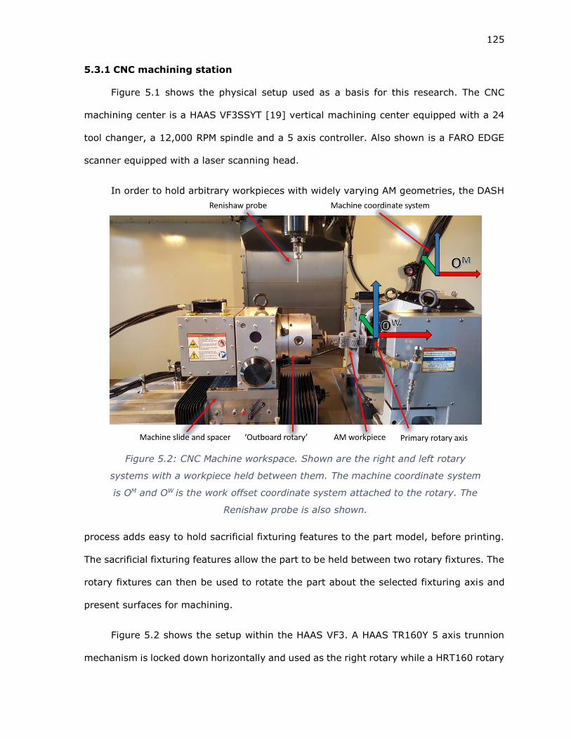
125

5.3.1 CNC machining station

Figure 5.1 shows the physical setup used as a basis for this research. The CNC

machining center is a HAAS VF3SSYT [19] vertical machining center equipped with a 24

tool changer, a 12,000 RPM spindle and a 5 axis controller. Also shown is a FARO EDGE

scanner equipped with a laser scanning head.

In order to hold arbitrary workpieces with widely varying AM geometries, the DASH

process adds easy to hold sacrificial fixturing features to the part model, before printing.

The sacrificial fixturing features allow the part to be held between two rotary fixtures. The

rotary fixtures can then be used to rotate the part about the selected fixturing axis and

present surfaces for machining.

Figure 5.2 shows the setup within the HAAS VF3. A HAAS TR160Y 5 axis trunnion

mechanism is locked down horizontally and used as the right rotary while a HRT160 rotary

Figure 5.2: CNC Machine workspace. Shown are the right and left rotary

systems with a workpiece held between them. The machine coordinate system

is OM and OW is the work offset coordinate system attached to the rotary. The

Renishaw probe is also shown.

126

axis is used as the outboard support. In an earlier version of this setup shown in Figure

5.5, a passive rotary was used as the outboard rotary axis. The outboard support may be

moved along the X axis to enable workpieces of varying lengths to be accommodated. The

two rotary axis were carefully aligned to be coaxial by means of spacer blocks, shims and

manual alignment. Figure 5.2 also shows the machine coordinate system OM as well as

the work offset coordinate system OW

5.3.2 3D Scanning systems

Two separate 3D scanning systems were employed in this effort. A FARO Edge Arm

[20] as shown in Figure 5.1, as well as a NextEngine HD [21], shown in Figure 5.3. The

NextEngine scanner is a relatively low end laser line scanning system with a specified

accuracy of ± 0.38 𝑚𝑚 [ ±0.015𝑖𝑛 ]. The laser emitter array in the NextEngine is panned in

order to capture surfaces in its field of view. The FARO Edge arm + scanner is a mid-range

system which also employs a laser line scanner as its sensing system. The scanning head

is connected to the main body of the scanner, containing the scanner’s coordinate system,

Figure 5.3: Setup with NextEngine HD mounted in CNC machine

127

by means of an articulated arm with 7 degrees of freedom. The scanning head must be

manually tracked across in order to capture a part’s surfaces. The articulated arm allows

for scanning within a hemisphere measuring 6 feet (1800 mm) across. The stated

repeatable accuracy of the FARO scanner is 0.034mm (0.0013in) over the entire

measurement hemisphere.

5.4 Approach

In order to generate a model of the workpiece as built and as mounted in the CNC

machine, multiple scans of the part must be transformed from the scanner coordinate

system to the work offset coordinate system corresponding to the fixture the workpiece

is affixed to. In the case of the setup described in Section 5.3A transform OS to OW, TS->W,

must be generated. In order to do this, we adopt the following approach:

a. Identify one or more fiducial features in the CNC machine coordinate system

Fiducial features may be formed by surfaces already in the CNC machine or

parts with fiducial features may be mounted in the CNC workspace, specifically

for this purpose.

Fiducial features must have simple geometries that are easy to localize by

traditional means

b. The geometry of a fiducial feature must uniquely define a coordinate system, OF

c. Measure and accurately locate the fiducial feature in the CNC machine workspace, in

the traditional manner.

This measurement is used to establish a transformation from the machine

coordinate system to the fiducial feature coordinate system TM->F

d. Mount the scanner at a position and orientation suitable for scanning both the part and

the fiducial feature.

The specific position is arbitrary and may be changed between parts or runs.

128

e. Scan both the fiducial feature as well as the part surfaces. If the CNC machine’s

position must be moved in order for all part surfaces to be scanned, record the CNC

machine position at which each scan is taken.

f. Use a suitable system to automatically detect the fiducial feature in the scan data and

compute the relative transformation from the scanner coordinate system to the fiducial

feature coordinate system, TS->F

g. The transformation from the scanner coordinate system to the machine coordinate

system can now be computed as TS->M = (TF->M) x (TS->F)

TF->M is simply the inverse of TM->F , (TM->F)-1, established in step #2.

TM->F may vary based on the commanded position of the CNC machine. For

example, if OF is attached to a rotary axis.

The transform from the machine coordinate system to the workspace coordinate

system, TM->W, is usually well known. The scanner to workspace transform TS->W can then

be established by applying TM->W by pre-multiplication The final form of the transformation

equation is given in Equation ( 5 ). Figure 5.4: Coordinate system transform sequence

shows the coordinate system transforms, overlaid over an image of the setup.

𝑇𝑆→𝑊 = 𝑇𝑀→𝑊 × (𝑇𝑀→𝐹)−1 × 𝑇𝑆→𝐹 ( 5 )

In Equation ( 5 ):

S denotes the scanner coordinate system

W denotes the workspace coordinate system

M denotes the machine coordinate system

F denotes the fiducial feature coordinate system

Based on the characteristics of the scanning system, this approach may be applied

in one of two ways. In the first method, registration is performed on a per scan basis. For

each captured scan, the fiducial features are detected, the registration transform is

129

computed and the scan is transformed to the workspace coordinate system. This method

is suitable for scanners that must be repositioned in order to capture a part’s surfaces,

such as the NextEngine.

In the second method, the scanner is fixed at suitable location and a scan is taken

of the fiducial feature. The registration transform, Equation ( 5 ), is extracted from this

scan. Multiple scans of the part are then taken and this same registration transformation

is applied to each of them in order to register them to the workspace coordinate system.

This approach is suitable for scanning systems such as the FARO Edge Arm, which need

not be moved to scan part surfaces due to the reach offered by the articulated arm.

Both methods were implemented, the first with the NextEngine scanner and the

second with the FARO Arm. The following sections describe the implementation of these

two approaches. Section 5.5 deals with a per-scan automatic registration system while

5.6 presents a system for registration by locating a fixed scanner by the measurement of

datum surfaces in the CNC machine. Each section contains a description of the system

Figure 5.4: Coordinate system transform sequence

130

and the algorithms used as well as experiments carried out to test each system’s ability

to successfully register scans.

5.5 Per-Scan Registration

The NextEngine 3D scanner can only capture objects in its field of view and must

therefore be repeatedly repositioned in order to capture all part surfaces. An

implementation of the strategy outlined in Section 5.4was developed to suit these

requirements.

The work described in this section is reproduced from a published paper entitled

“Automatic Part Localization in a CNC Machine Coordinate System by Means of 3D Scans.”

In the International Journal of Advanced Manufacturing Technology [22].

5.5.1 Fiducial Features

As the NextEngine scanner must be re-positioned in order to capture scans, a fiducial

feature may be occluded by the setup or the workpiece, depending on the position. In

order to address this, multiple fiducial features are mounted in the setup and the

processing software is designed to automatically detect the best candidate feature that is

visible in the scan. Figure 5.5 shows the setup in the CNC Machine with two prismatic

blocks that each have a fiducial feature machined into them.

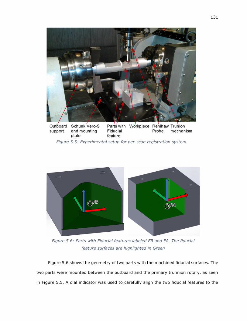
131

Figure 5.6 shows the geometry of two parts with the machined fiducial surfaces. The

two parts were mounted between the outboard and the primary trunnion rotary, as seen

in Figure 5.5. A dial indicator was used to carefully align the two fiducial features to the

Figure 5.5: Experimental setup for per-scan registration system

Figure 5.6: Parts with Fiducial features labeled FB and FA. The fiducial

feature surfaces are highlighted in Green

132

axes of the CNC machine and their positions were recorded by probing the three planes

that form each fiducial feature. In order to improve visibility to the scanner and to reduce

reflections, both fiducial features were sand-blasted.

5.5.2 Registration algorithm

The software for automatically detecting the fiducial features and computing the

transforms is written in C++ with the aid of the PCL library [23].

In this system, the fiducial features are detected in the scan data by attempting to

find and fit a model of the fiducial feature, located in its own coordinate system to the

scan data. If the fit is successful, the transformation that resulted in the fit is TF->S. The

transformation from the fiducial feature coordinate system to the scanner coordinate

system. TS->F, required for Equation ( 5 ) is simply (TF->S)-1.

The software system requires point models (point clouds) of the fiducial features for

this fitting procedure. The point models were created using Meshlab [24] by extracting

and sampling the cad model surfaces using a Poisson Disc Sampling filter, with a sampling

radius of 0.5mm, i.e. the mean distance between sampled points was 0.5mm.

A two stage system for fitting the sampled point models of the fiducial features to

the scan data is used. In the first stage, the Sample Consensus Initial Alignment (SAC-

IA) algorithm from the PCL library [25] is used to approximately fit the model to the scan

data. Following this, the Iterative Closest Points algorithm (ICP) is used to refine the fit.

Figure 5.7 shows the two stage fit process. The point model of the fiducial features is in

Red and the scanned point cloud is in Grey.

133

5.5.2.1 Selection of best fiducial feature

Since multiple fiducial features are present in the scan data, it is necessary to select

the best fiducial feature to fit against, accounting for occlusions and visibility from the

scanner’s current pose. This is performed by successively attempting to fit each fiducial

feature model to the scan data and computing a metric representing the success of a fit.

Fiducial feature models that successfully fit to the scan data will score highly on this metric,

while a poor score indicates a bad fit. Equation ( 6 ) shows the metric used to measure

the success of the fit.

Nf

∑(𝑃𝑓𝑃𝑠𝑓)

( 6 )

Figure 5.7: Two stage fit process. (a) shows the sampled point model of the

fiducial feature in Red. (b) shows a sample of a scan taken by the NextEngine in

Grey. (c) shows the approximate fit using SAC-IA (d) shows the refined fit using

the ICP algorithm.

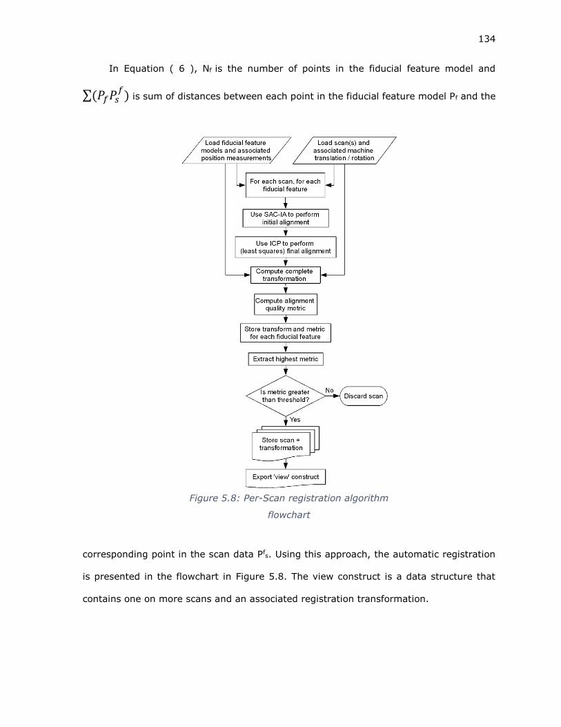
134

In Equation ( 6 ), Nf is the number of points in the fiducial feature model and

∑(𝑃𝑓𝑃𝑠𝑓) is sum of distances between each point in the fiducial feature model Pf and the

corresponding point in the scan data Pfs. Using this approach, the automatic registration

is presented in the flowchart in Figure 5.8. The view construct is a data structure that

contains one on more scans and an associated registration transformation.

Figure 5.8: Per-Scan registration algorithm

flowchart

135

5.5.3 Experimental design

In order to test the ability of the system described here to successfully register

scans, a machined test workpiece, shown in Figure 5.9, was manufactured and mounted

between centers in the CNC machine. The test workpiece was shimmed to simulate

misalignment due to rough AM surfaces. Six scans were taken of the part, at chuck

rotations of 0, 45 and 90 degrees from two scanner poses. These scans were automatically

stitched together taken using the system described in section 5.5.2. The combined point

model from these six scans was clipped and down-sampled to reduce the density of the

scan data, and generate a combined point model of the workpiece as built and as it is

mounted in the CNC machine, seen in Figure 5.10.

Figure 5.9: Test workpiece. Image on right shows shims to simulate

misalignment as well as Renishaw probe, used to measure workpiece test

surfaces.

Figure 5.10: Combined point cloud

136

The test workpiece was manufactured to have a set of reference surfaces shown

and highlighted in Figure 5.11. In order to measure the in-machine location and position

of this workspace coordinate system, a point model of the reference surfaces was

generated and transformed to fit the combined scan model from Figure 5.10. This was

performed using the ICP algorithm. No initial alignment was necessary as the deviation

from nominal to as-mounted location in the CNC machine was sufficiently small. The

flowchart in Figure 5.12 shows the sequence of steps followed.

This procedure was performed 5 times, with the workpiece shimmed differently each

time, simulating the varying misalignments. After each test, the ‘true’ position of the test

workpiece reference surfaces were measured by means of the Renishaw Probe, as seen in

Figure 5.9. Since the Renishaw probe has a significantly better accuracy rating than the

laser scanner, the position estimated through probing was treated as the ‘true’ position.

Figure 5.11: Test workpiece with reference surfaces

highlighted in green. The coordinate system OP is attached

to and constructed from the reference surfaces

137

5.5.4 Results

The results of the 5 experimental tests are presented in Table 5.1. Table 5.2 shows

the mean and standard deviation of the registration error in the three cardinal directions

as well as the overall 2-norm of the error - the distance between the origins of OP as-

probed and as-scanned.

Figure 5.12: Sequence of steps used to create a

combined model of the test workpiece and to

extract its true position in the CNC machine

138

The errors recorded here are in line with the stated accuracy of the scanner. This

shows that the per-scan registration scheme presented here is capable of registering data

to the accuracy of the underlying scan data.

5.6 Registration through estimation of fixed scanner pose

5.6.1 Observations from Per-Scan Registration system

While the per-scan registration system described in the previous section has been

demonstrated to be successful, several challenges remain to be solved. The first challenge

is the accuracy of the overall system. This is driven primarily by the scanner performance,

and can be solved with a scanning system that meets the required accuracy specification.

The second challenge is the requirement for parts with fiducial feature geometries to be

mounted in the CNC machine space. In many machine configurations, there is no

Table 5.1: Experimental results. XM etc refer to measured (true) coordinates while

XL etc refer to the coordinates as located by the scan based localization system. All

units are in mm

Test # XM XL YM YL ZM ZL αM αL βM βL γM γL

1 -77.47 -77.52 -12.79 -13.00 20.67 20.99 0.5 0.7 -0.1 0.0 0.0 0.2

2 -80.06 -80.13 -10.41 -10.95 21.08 21.49 -6.8 -6.6 0.1 0.2 0.0 0.0

3 -78.81 -78.91 -12.16 -12.44 20.31 20.63 -1.9 -1.9 0.3 0.4 0.0 0.0

4 -80.90 -80.97 -11.59 -12.01 21.71 22.11 -3.1 -3.0 0.0 0.0 0.0 0.1

5 -78.78 -78.85 -13.86 -14.16 19.75 20.03 4.0 4.2 0.0 0.0 0.0 0.3

Dimension Average Error (mm) Standard deviation

X 0.07 0.6

Y 0.35 0.13

Z 0.35 0.02

||X ,Y, Z|| 0.502 0.12

Table 5.2: Mean system performance

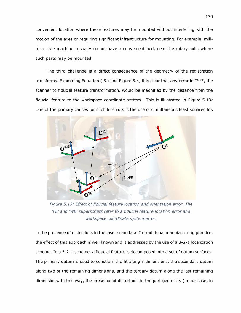
139

convenient location where these features may be mounted without interfering with the

motion of the axes or requiring significant infrastructure for mounting. For example, mill-

turn style machines usually do not have a convenient bed, near the rotary axis, where

such parts may be mounted.

The third challenge is a direct consequence of the geometry of the registration

transforms. Examining Equation ( 5 ) and Figure 5.4, it is clear that any error in TS->F, the

scanner to fiducial feature transformation, would be magnified by the distance from the

fiducial feature to the workspace coordinate system. This is illustrated in Figure 5.13/

One of the primary causes for such fit errors is the use of simultaneous least squares fits

in the presence of distortions in the laser scan data. In traditional manufacturing practice,

the effect of this approach is well known and is addressed by the use of a 3-2-1 localization

scheme. In a 3-2-1 scheme, a fiducial feature is decomposed into a set of datum surfaces.

The primary datum is used to constrain the fit along 3 dimensions, the secondary datum

along two of the remaining dimensions, and the tertiary datum along the last remaining

dimensions. In this way, the presence of distortions in the part geometry (in our case, in

Figure 5.13: Effect of fiducial feature location and orientation error. The

‘FE’ and ‘WE’ superscripts refer to a fiducial feature location error and

workspace coordinate system error.

140

the scan data) do not cause the fit system to ‘fight itself’ – where a better fit to one surface

reduced the quality of the fit to another.

Combining these three Observations, the following approach is adopted for a new

registration scheme.

a. The NextEngine scanner is replaced with the FARO Edge ScanArm

b. The chuck body is used as a fiducial feature

c. Instead of a simultaneous ‘best-fit’ with a point model of the fiducial feature, each

datum surface of the chuck is extracted and used to constrain appropriate degrees of

freedom, similar to a 3-2-1 fitting system.

5.6.2 Chuck geometry and datums

Figure 5.14 shows a model of a generic 3 jaw chuck and the associated axes, as the

chuck is mounted in the setup. Figure 5.15 shows the datum surfaces on the chuck. The

cylindrical body of the chuck is the primary datum and is used to constrain the Y and Z

Figure 5.14: Chuck and axes

141

positions as well as the X axis of the work coordinate system attached to the chuck. The

face of the chuck is the secondary datum, and is used to constrain the X coordinate. The

Y axis of the coordinate system is defined as being simultaneously perpendicular to the X

axis and parallel to the plane defined by the face of Jaw #1. The Z axis is constructed

from the X and Y axes using the right hand rule.

In practice, the chuck is mounted in the CNC machine and carefully aligned to lie

parallel to the CNC machine axes. This fixes the X and Y axis of the chuck. The body of

the chuck is then used to ensure that the chuck and rotary axis are coincident, by moving

the chuck to eliminate any runout. The chuck face is then measured to determine the X

coordinate of the work offset attached to the chuck. The chuck is then rotated until the

top face of Jaw #1 lies parallel to the XY plane. This rotation is recorded as the Alpha 0 of

the work offset. Finally, the center of rotation of the chuck is measured and recorded as

Figure 5.15: Chuck datums. The Chuck Body Cylinder is the primary

Datum, colored Red; The Chuck Face is the secondary datum, in green;

Jaw #1 Face is tertiary datum, colored blue. Jaws #2 and #3 are hidden,

for clarity

142

the Y and Z position of the work offset, in the CNC machine coordinate system. In many

cases the work offset is moved along X to sit at the face of a jaw.

5.6.3 Registration algorithm

5.6.3.1 Registration transform from chuck coordinate system

In order to determine TS->FC, the transform from the scanner coordinate system to

the chuck coordinate system (FC = fiducial feature, chuck) the origin and axis of the

coordinate system formed by the chuck datum surfaces must be extracted in the scanner

coordinate system, from the scan data.

Given the orthogonal unit vectors corresponding to the X, Y and Z axis and the origin

O of the chuck work offset coordinate system, as observed in the scanner frame of

reference, the registration transformation is simply the inverted matrix shown in Equation

( 7 ). In Equation ( 7 ), the superscript ‘c’ is used to denote ‘chuck’.

[ Xi

c 𝑌𝑖𝑐 𝑍𝑖

𝑐 𝑂𝑥𝑐

X𝑗c 𝑌𝑗

𝑐 𝑍𝑗𝑐 𝑂𝑦

𝑐

𝑋𝑘𝑐 𝑌𝑘

𝑐 𝑍𝑘𝑐 𝑂𝑧

𝑐

0 0 0 1 ] −1

( 7 )

The challenge then is to extract this information from the scan data.

5.6.3.2 Extraction of geometric models from point clouds – RANSAC

Extracting geometrical shapes from noisy real world scan data (point clouds) can be

performed by many means. One of the most popular techniques is the RANdom SAmple

Consensus algorithm (RANSAC) [26]. The RANSAC algorithm functions by attempting to

divide an input dataset into two subsets – a set of ‘inliers’ that correspond to a geometrical

shape present in the input data and a set of ‘outliers’ that do not.

The RANSAC algorithm requires a model construct of the required geometry that is

capable of performing two functions:

143

a. Given a set of points in space, compute the parameters of a geometric model

that fits those points.

The RANSAC model must specify the number of points required. For

example, a RANSAC Plane model will require three points in order to

compute a unique plane

The RANSAC model may also indicate that a suitable model could not be

constructed from the given data. For example, if the three points provided

to a RANSAC plane model are collinear or the diameter of a cylinder

computed by a RANSAC cylinder model falls outside the acceptable limits.

b. Given a model and a data set, to compute the subset of points that are

considered inliers.

Given such a model, the RANSAC algorithm performs the following sequence of steps:

a. From a given data set, a set of samples is selected at random.

The number of samples equals the number required by the RANSAC

model being used

b. The RANSAC model is then used to test the validity of the selected samples and

compute a candidate geometric model.

c. Given a successfully computed geometry model, the number of points in the

full data set that are considered ‘inliers’ is counted

d. The sequence of steps 1 through 3 is repeated many times. The candidate

model that resulted in the greatest number of inliers is considered to be the

model that best fits the data set.

In common practice, a least squares fit against the entire set of inliers is used to

refine the candidate model. Subsequent to this, the set of inliers is removed from the data

set and the data set may be further processed to find other geometries that may be

present in it.

144

5.6.4 RANSAC Implementation

This system was implemented in C++ with the aid of the PCL and Eigen libraries

[27]. The pcl::RandomSampleConsensus implementation of the RANSAC algorithm was

used, together with several RANSAC model types, detailed in the following subsections.

5.6.4.1 Chuck body extraction

In order to extract the chuck Body, a cylinder RANSAC model from the PCL library,

pcl::SampleConsensusModelCylinder is used. This model requires two points (with

normals) to compute a candidate cylinder model. This model also supports the

specification of maximum and minimum acceptable diameters, in order to limit the

candidate set of cylinders detected to those actually being searched for.

The pcl::SampleConsensusModelCylinder RANCAC model selects inliers by testing a

combination of distance from the surface of the candidate cylinder as well as the angular

deviation of the test point normal from the radial vector of the candidate cylinder. Equation

( 8 ) shows the inlier acceptance metric used by this RANSAC model. 𝐷𝜃 is the angle

between the point normal and the vector from the point to its projection on the cylinder

axis. 𝐷𝑒 is the distance from the point position to the candidate cylinder surface? ‘w’ is a

weighing factor 0 ≤ 𝑤 ≤ 1 between angular and positional distances. The library default w

value of 0.1 was used throughout this work.

𝑤 × 𝐷𝜃 + (1 − 𝑤) × 𝐷𝑒 < 𝑡ℎ𝑟𝑒𝑠ℎ𝑜𝑙𝑑 ( 8 )

Subsequent to the extraction of the set on inliers, the cylinder model is refined by

performing a least squares fit with the entire set of inliers.

5.6.4.2 Extraction of Chuck Face and Jaw

When using a 3-2-1 fit in traditional practice, the primary datum may be found using

all available degrees of freedom. The secondary datum must be located and measured

145

while constrained to be perpendicular to the primary datum. The tertiary datum must be

located and measured while constrained to be perpendicular to the primary datum.

Since the chuck face and jaw are secondary and tertiary datums, respectively, it is

necessary to force the RANSAC system to search exclusively for appropriately constrained

plane features in the scan data. In order to perform this, a custom RANSAC model was

developed – the directed normal plane.

The directed normal plane requires three sample points in order to compute a

candidate plane model. The normal direction of the candidate plane model is flipped to

match the average normal direction of the three samples.

The directed normal plane has two modes for testing validity – normal parallel and

normal perpendicular. In both cases the model is provided with a desired axis and a

threshold angle. In the normal parallel case, the model is considered valid if the candidate

model plane normal is within ‘threshold degrees’ of the desired axis, in the normal

perpendicular case, the model is considered valid only if the plane normal is within

‘threshold degrees’ of an axis perpendicular to the candidate axis.

Once a valid candidate model has been created, inliers are selected based on both

position and normal direction criteria. For a point to be an inlier, it must (a) lie within a

selected threshold distance of the candidate plane model and (b) the point normal must

be within a threshold of the plane normal.

While the datum surfaces of a chuck are precision ground and suitable as a basis for

registration, they often feature embossed or debossed writing of manufacturer

information, serial number etc stamped onto their surfaces. When manually locating a

chuck, an operator can easily avoid these regions by visual inspection, in order to prevent

erroneous measurements. When automatically detecting geometric features in point cloud

data, however, this must be performed algorithmically. The rejection of writing on chuck

146

datum surfaces is achieved in the directed normal plane RANSAC model by means of the

normal angle threshold in inlier selection. Since point cloud normals are computed by

analyzing a point neighborhood, any points near a distorted surface, due to embossing or

debossing, will have a normal direction that deviates from plane normal and will

consequently be rejected.

Subsequent to the extraction of the set on inliers, the plane model is refined by

performing a least squares fit with the entire set of inliers.

5.6.5 Procedure for Chuck Pose detection

In order to detect the chuck datum surfaces a scan is taken of the chuck, that

includes the chuck body, the chuck face and Jaw #1. Since the RANSAC algorithm searches

for models with the maximum number of inliers, care should be taken to minimize the

presence of extraneous surfaces such as faces on the part, other fixtures in the CNC

machine or Jaw side surfaces other than the selected datum in the scan data. Figure 5.16

shows the sequence of steps used to detect the features of the chuck. At each stage, the

inliers found for the final detected candidate model, are removed from the scanned point

cloud prior to searching for the next geometric shape.

The Y and Z coordinates of the cylinder axis point (a point-direction-radius scheme

is used to define the cylinder) are used as the Y and Z coordinates of the chuck coordinate

system. The chuck axis direction is used as the X axis. The X coordinate is computed as

the intersection of the chuck face plane with the A axis. In order to compute the Y axis,

the cross producer of the Jaw plane normal with the A axis is taken. This gives us a Y axis

that is constrained to lie perpendicular to the A axis as well as the Jaw plane. Finally, the

Z axis is computed by the cross product of the extracted X and Y axes. The axis and

147

coordinate information is used to construct the registration transformation, as shown in

Equation ( 7 )

Figure 5.16: Algorithm for chuck pose extractions

148

Figure 5.17 shows an example chuck scan with 1.07 million points. Care was taken

to ensure that datum surfaces were preferred over non-datum surfaces when scanning

was performed. Figure 5.19 shows the extracted datum surfaces (set of inliers) and a

constructed coordinate system. The extracted chuck body has ~400,000 points, the

extracted chuck face ~200,000 points and the extracted jaw ~100,000 points. Figure 5.18

shows the rejection of ‘bad’ regions on the datum surfaces, corresponding to writing or

bolts holes.

Figure 5.17: Example scan of chuck with 1.07 million points.

149

Figure 5.19: Extracted Datums. Chuck Body Cylinder in Red, Chuck

Face in Green and Jaw in Blue.

Figure 5.18: Rejection of ‘bad’ regions. Regions circled in

white represent regions on the datum surfaces where points

were rejected by the RANSAC system

150

5.6.6 Experimental design

The following approach is traditionally used to validate the accuracy of a chuck’s

measured position in a CNC machine:

a. A piece of stock is mounted in the chuck

b. The CNC machine is used to machine a flat plane in the stock, parallel to the YZ plane

and at a fixed offset, O, from the chuck axis.

c. The chuck is rotated 180 degrees and a similar flat plane is again cut in the stock, at

the same fixed offset O.

d. The true plane – plane distance, M, is measured.

The error in the located position of the chuck is (O – M/2).

Building on this technique, the following approach is taken to conduct a preliminary

validation of the performance this registration system.

The chuck datums are detected and the registration transform is computed in the

manner described above.

Figure 5.20: Procedure for measuring the accuracy with which a chuck is located.

True axis and Expected planes are shown in green, the measured axis and planes as

produced are shown in orange

151

1. Two precision ground, anti-parallel, planar surfaces, attached to the chuck are

scanned at rotations 180 degrees apart

2. The registration transformation is used to reconstruct a combined point cloud

incorporating both planar surfaces at as located with respect to the chuck

coordinate system

3. Geometric plane models are fit to the registered planes

4. The positional error, between the two plane surfaces is measured

5. As with the traditional approach, the positional inaccuracy is half the difference

between the true and as-scanned plane-plane distance.

The ground surfaces selected for this experiment were the parallel surfaces of chuck

jaw #2. Figure 5.22 through Figure 5.25 show this procedure. Prior to testing, the chuck

was carefully aligned with the rotary axis in order to ensure that all observed errors were

purely the result of inaccuracy in scanning.

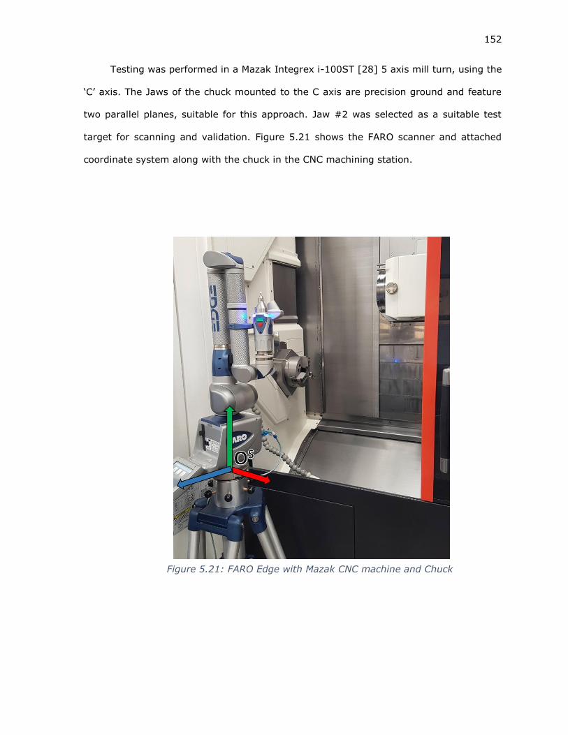
152

Testing was performed in a Mazak Integrex i-100ST [28] 5 axis mill turn, using the

‘C’ axis. The Jaws of the chuck mounted to the C axis are precision ground and feature

two parallel planes, suitable for this approach. Jaw #2 was selected as a suitable test

target for scanning and validation. Figure 5.21 shows the FARO scanner and attached

coordinate system along with the chuck in the CNC machining station.

Figure 5.21: FARO Edge with Mazak CNC machine and Chuck

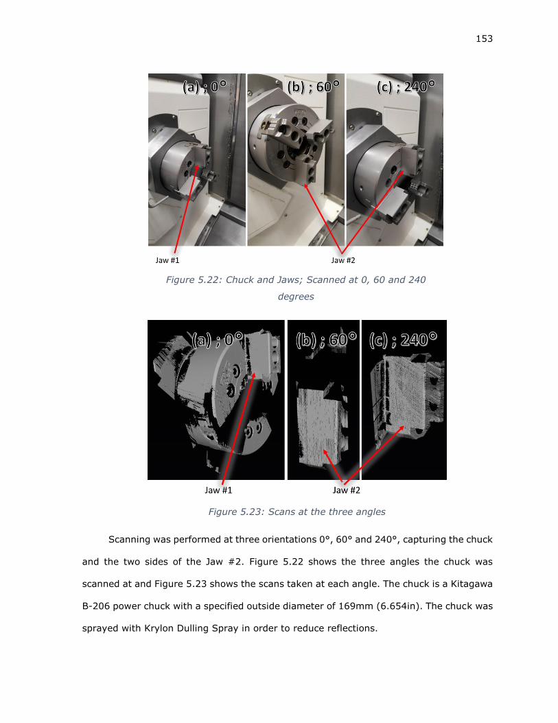
153

Scanning was performed at three orientations 0°, 60° and 240°, capturing the chuck

and the two sides of the Jaw #2. Figure 5.22 shows the three angles the chuck was

scanned at and Figure 5.23 shows the scans taken at each angle. The chuck is a Kitagawa

B-206 power chuck with a specified outside diameter of 169mm (6.654in). The chuck was

sprayed with Krylon Dulling Spray in order to reduce reflections.

Figure 5.22: Chuck and Jaws; Scanned at 0, 60 and 240

degrees

Figure 5.23: Scans at the three angles

154

Using the registration system presented, the chuck datum surfaces were extracted,

a registration transformation was created and the two scans of the jaws were registered

to the chuck coordinate system (and, in effect, to each other). Figure 5.24 shows a

combined, registered model.

The two parallel sides of the Jaw were then analyzed, and the plane-plane distance

as well as angle was extracted. This procedure was repeated 4 times. Table 5.3 shows the

critical dimensions of the chuck and jaw, as well as the RANSAC and Scanning parameters

used.

Figure 5.24: Combined model of Jaw #2, Registered to

the chuck coordinate system

155

The wall to wall width of the Jaw in each combined scan was measured by fitting

parallel planes to the point cloud using Geomagic Qualify 2012. Acceptable deviation

threshold parameters of 0.004” inches (0.10 mm) and 2 degrees were used for the fit.

Figure 5.25 Shows the fitting of two parallel planes to the walls of the scanned Jaw.

Figure 5.25: Fitting of parallel planes to Jaw in Geomagic

Qualify 2013

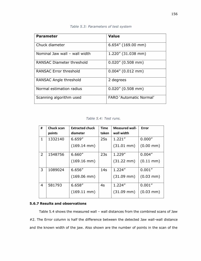
156

5.6.7 Results and observations

Table 5.4 shows the measured wall – wall distances from the combined scans of Jaw

#2. The Error column is half the difference between the detected Jaw wall-wall distance

and the known width of the jaw. Also shown are the number of points in the scan of the

Table 5.3: Parameters of test system

Parameter Value

Chuck diameter 6.654” (169.00 mm)

Nominal Jaw wall – wall width 1.220” (31.038 mm)

RANSAC Diameter threshold 0.020” (0.508 mm)

RANSAC Error threshold 0.004” (0.012 mm)

RANSAC Angle threshold 2 degrees

Normal estimation radius 0.020” (0.508 mm)

Scanning algorithm used FARO ‘Automatic Normal’

Table 5.4: Test runs.

# Chuck scan

points

Extracted chuck

diameter

Time

taken

Measured wall-

wall width

Error

1 1332140 6.659”

(169.14 mm)

25s 1.221”

(31.01 mm)

0.000”

(0.00 mm)

2 1548756 6.660”

(169.16 mm)

23s 1.229”

(31.22 mm)

0.004”

(0.11 mm)

3 1089024 6.656”

(169.06 mm)

14s 1.224”

(31.09 mm)

0.001”

(0.03 mm)

4 581793 6.658”

(169.11 mm)

4s 1.224”

(31.09 mm)

0.001”

(0.03 mm)

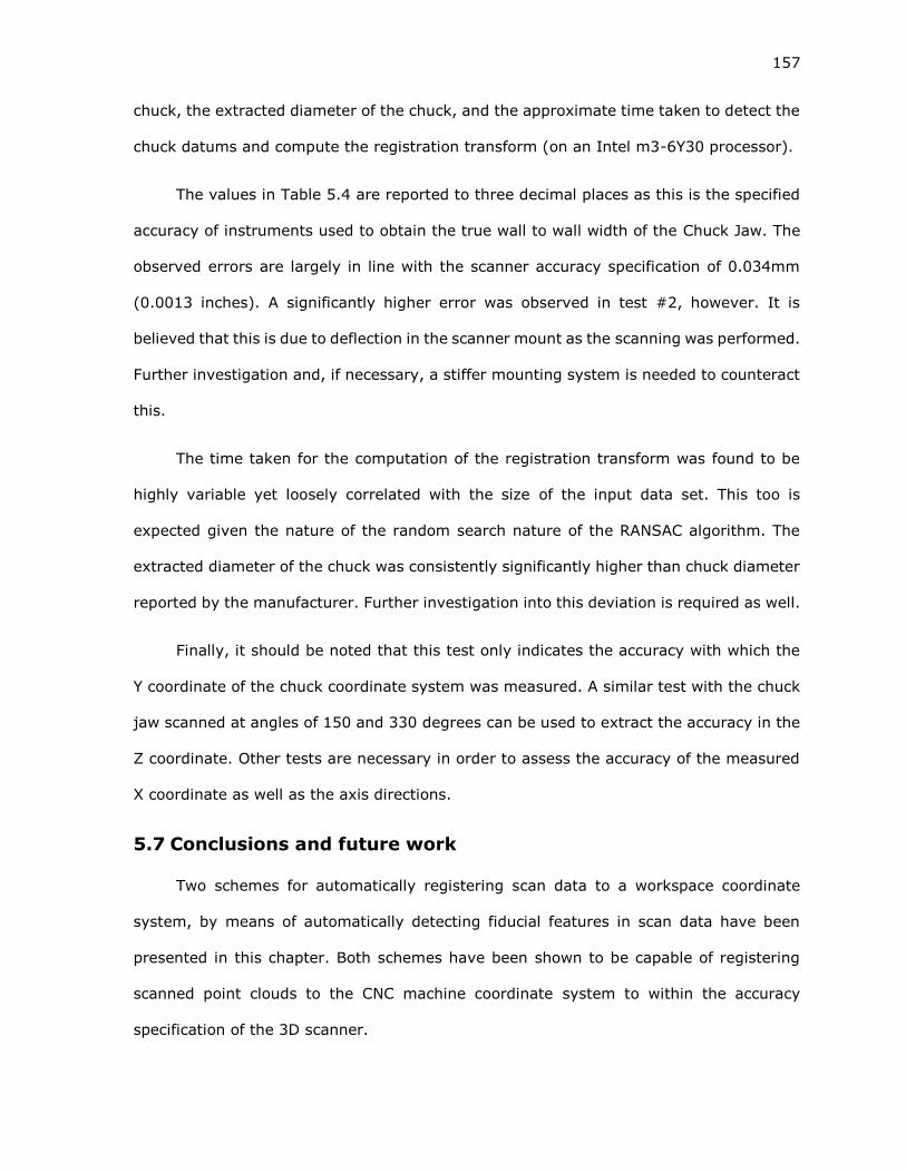
157

chuck, the extracted diameter of the chuck, and the approximate time taken to detect the

chuck datums and compute the registration transform (on an Intel m3-6Y30 processor).

The values in Table 5.4 are reported to three decimal places as this is the specified

accuracy of instruments used to obtain the true wall to wall width of the Chuck Jaw. The

observed errors are largely in line with the scanner accuracy specification of 0.034mm

(0.0013 inches). A significantly higher error was observed in test #2, however. It is

believed that this is due to deflection in the scanner mount as the scanning was performed.

Further investigation and, if necessary, a stiffer mounting system is needed to counteract

this.

The time taken for the computation of the registration transform was found to be

highly variable yet loosely correlated with the size of the input data set. This too is

expected given the nature of the random search nature of the RANSAC algorithm. The

extracted diameter of the chuck was consistently significantly higher than chuck diameter

reported by the manufacturer. Further investigation into this deviation is required as well.

Finally, it should be noted that this test only indicates the accuracy with which the

Y coordinate of the chuck coordinate system was measured. A similar test with the chuck

jaw scanned at angles of 150 and 330 degrees can be used to extract the accuracy in the

Z coordinate. Other tests are necessary in order to assess the accuracy of the measured

X coordinate as well as the axis directions.

5.7 Conclusions and future work

Two schemes for automatically registering scan data to a workspace coordinate

system, by means of automatically detecting fiducial features in scan data have been

presented in this chapter. Both schemes have been shown to be capable of registering

scanned point clouds to the CNC machine coordinate system to within the accuracy

specification of the 3D scanner.

158

This approach for registering scan data has utility wherever a scanning system may

be used to detect the geometry and pose of a workpiece in a workspace coordinate system.

Examples include the finish machining of castings and forgings as well as in high

performance metrology systems such as Coordinate Measuring Machines and industrial

XRay system, to provide a preliminary geometry model for targeted inspection planning.

5.7.1 Future work

The most important future work necessary is the creation of a comprehensive

mathematical model for the propagation of errors in scanning, datum extraction and

registration. Such a system would need to be capable of quickly analyzing the data

gathered together with the extracted datums and assessing the quality of the generated

registration transformation. This performance analysis could then be used provide

feedback to the operator and perhaps to indicate if further scanning is required for a

sufficiently accurate transform.

Improvements to the performance of the extraction algorithm are also an important

future goal. While the current system is fast enough for practical use (under one minute

on a laptop with a consumer grade intel processor), a significantly faster system would

enable real-time feedback and refinement of fit. This would in turn reduce the required

operator skill levels when a manually operated scanning system like the FARO arm is

employed.

The current system requires the programmatic specification of datum surfaces and

the sequence in which they must be extracted and used. A graphic user environment

which allows users to specify geometric features, expected to be present in scan data, as

datums for automatic detection is necessary for the deployment of this system in industry.

159



[2] Renishaw, “Renishaw | Probing systems and software,” 2014. [Online]. Available:

http://www.renishaw.com/en/probing-systems-and-software--12466. [Accessed:

13-Nov-2014].

[3] P. J. Besl and N. D. McKay, “Method for registration of 3-D shapes,” presented at the

SPIE, 1992, vol. 1611, pp. 586–606.

[4] R. B. Rusu, “Semantic 3D object maps for everyday manipulation in human living

environments,” KI-Künstl. Intell., vol. 24, no. 4, pp. 345–348, 2010.

[5] N. Gelfand, N. J. Mitra, L. J. Guibas, and H. Pottmann, “Robust Global Registration.,”

in Symposium on geometry processing, 2005, vol. 2, p. 5.

[6] R. L. Aman, “A Minimal Surface Perturbation Method for Global Surface Registration

of Unstructured Point Cloud Data.,” 2004.

[7] S. J. Gordon and W. P. Seering, “Real-time part position sensing,” IEEE Trans. Pattern

Anal. Mach. Intell., vol. 10, no. 3, pp. 374–386, 1988.

[8] G. Biegelbauer and M. Vincze, “3D Vision-Guided Bore Inspection System,” in IEEE

International Conference on Computer Vision Systems, 2006 ICVS ’06, 2006, pp. 22–

22.

[9] O. Skotheim, M. Lind, P. Ystgaard, and S. A. Fjerdingen, “A flexible 3D object

localization system for industrial part handling,” in 2012 IEEE/RSJ International

Conference on Intelligent Robots and Systems (IROS), 2012, pp. 3326–3333.

[10] M. Rajaraman, M. Dawson-Haggerty, K. Shimada, and D. Bourne, “Automated

workpiece localization for robotic welding,” in 2013 IEEE International Conference on

Automation Science and Engineering (CASE), 2013, pp. 681–686.

[11] K. Okarma and M. Grudzinski, “The 3D scanning system for the machine vision based

positioning of workpieces on the CNC machine tools,” in 2012 17th International

Conference on Methods and Models in Automation and Robotics (MMAR), 2012, pp.

85–90.

[12] D. Starr, “Method and apparatus for singulating, debarking, scanning and

automatically ...,” 6539993, 01-Apr-2003.

160

[13] J. R. McCown and J. R. Firth, “Small log bucking system,” 4468993, 04-Sep-1984.

[14] J. E. Hards, “Sweep-data-responsive, high-speed, continuous-log-travel bucking

apparatus,” 4640160, 03-Feb-1987.

[15] K. Pathak, N. Vaskevicius, J. Poppinga, M. Pfingsthorn, S. Schwertfeger, and A. Birk,

“Fast 3D mapping by matching planes extracted from range sensor point-clouds,” in

IEEE/RSJ International Conference on Intelligent Robots and Systems, 2009. IROS

2009, 2009, pp. 1150–1155.

[16] K. Pathak, A. Birk, N. Vaskevicius, M. Pfingsthorn, S. Schwertfeger, and J. Poppinga,

“Online three-dimensional SLAM by registration of large planar surface segments and

closed-form pose-graph relaxation,” J. Field Robot., vol. 27, no. 1, pp. 52–84, Jan.

2010.

[17] J. Poppinga, N. Vaskevicius, A. Birk, and K. Pathak, “Fast plane detection and

polygonalization in noisy 3D range images,” in Intelligent Robots and Systems, 2008.

IROS 2008. IEEE/RSJ International Conference on, 2008, pp. 3378–3383.

[18] A. J. B. Trevor, J. G. Rogers, and H. I. Christensen, “Planar surface SLAM with 3D

and 2D sensors,” in 2012 IEEE International Conference on Robotics and Automation

(ICRA), 2012, pp. 3041–3048.

[19] Haas, “Haas VF-3 | Haas Automation®, Inc. | CNC Machine Tools,” 2014. [Online].

Available: http://www.haascnc.com/mt_spec1.asp?id=VF-

3&webID=40_TAPER_STD_VMC#gsc.tab=0. [Accessed: 01-Jul-2014].

[20] “Portable CMMs - Metrology Solutions from FARO.” [Online]. Available:

http://www.faro.com/products/metrology. [Accessed: 12-Apr-2016].

[21] NextEngine, “NextEngine 3D Laser Scanner,” 2014. [Online]. Available:

http://www.nextengine.com/. [Accessed: 01-Jul-2014].

[22] H. Srinivasan, O. L. A. Harrysson, and R. A. Wysk, “Automatic part localization in a

CNC machine coordinate system by means of 3D scans,” Int. J. Adv. Manuf. Technol.,

vol. 81, no. 5–8, pp. 1127–1138, May 2015.

[23] R. B. Rusu and S. Cousins, “3d is here: Point cloud library (pcl),” in Robotics and

Automation (ICRA), 2011 IEEE International Conference on, 2011, pp. 1–4.

[24] Visual Computing Lab ISTI - CNR, MeshLab. .

161

[25] R. B. Rusu, N. Blodow, and M. Beetz, “Fast Point Feature Histograms (FPFH) for 3D

registration,” in IEEE International Conference on Robotics and Automation, 2009.

ICRA ’09, 2009, pp. 3212–3217.

[26] M. A. Fischler and R. C. Bolles, “Random sample consensus: a paradigm for model

fitting with applications to image analysis and automated cartography,” Commun.

ACM, vol. 24, no. 6, pp. 381–395, 1981.

[27] G. Guennebaud and J. B. Eigen, A C++ template library for linear algebra. 2015.

[28] “INTEGREX i-100ST.” [Online]. Available:

https://www.mazakusa.com/machines/integrex-i-100st/. [Accessed: 25-Apr-2016].

162

Chapter 6

AUTOMATIC FEATURE-BASED LOCALIZATION

A near net shape workpiece mounted in the CNC machine will sit at a position and

orientation differing from its nominal pose due to imperfections in its datum surfaces. This

poses a challenge to finish machining. Traditionally, this is solved by locating the part

manually, or with fixtures. However, neither approach is suitable for AM parts that may

feature complicated geometries and small lot sizes. The solution is to obtain a model of

the part as built and as it is mounted in the CNC machine, and to use this model to find

an offset that shifts the nominal part model ‘within’ the detected material. Chapter 5

presented a methodology for the automatic registration of 3D scan data to the CNC

machine work coordinate system and thereby the creation of such a model. The objective

of this chapter is to present a methodology for the generation of an appropriate offset,

that moves the target model to a position and orientation at which it may be successfully

‘harvested’ from the workpiece material present.

6.1 Background and Motivation

In traditional casting practice, allowances are added to a part model, prior to casting,

to account for shrinkage during the casting process as well as for finish machining. A part

model with these allowances and offsets is referred to as ‘steel safe’. Once the casting

process is complete, the cast part (workpiece) is mounted in a CNC machine for finish

machining. When lot sizes are too low for the creation of specialized fixtures, such as with

prototypes, datum surfaces on the cast part are identified and used to locate and orient

the workpiece in the CNC machine space. Subsequent to this, the material that is to be

removed is ‘marked out’ by means of a scribe and measuring blocks, gages, calipers and

other instruments. The process of marking out a workpiece effectively ‘finds the final,

163

desired part’ within the material present and allows the machinist to visualize the regions

that are to be machined and to ensure that sufficient material is present for the successful

production of the final part.

In the context of the DASH process, the model of the part is represented as a

toleranced AMF (AMF-TOL) file and the stock model is available as a registered combined

point cloud. The challenge is to find a transformation that moves the part model inside

the point cloud, such that the features that are to be finish machined lie sufficiently ‘below’

the corresponding surfaces in the point cloud.

6.2 Literature review

The challenge of automatically determining the offsets at which a part should be

produced has been addressed by several authors.

Li et al. [1] present a comprehensive underlying theory for workpiece localization

and allowance assignment. In [1], the Hybrid Localization / Envelopment problem is

formulated and solved as a constrained least squares problem.

Identifying the challenges posed by manually marking out of castings, especially in

the presence of large defects in the near-net-shape workpieces and complicated

geometries, Gessner et al. [2] presented a method for the determination of the pose at

which a part must be machined, within a given blank. Multiple scans of the workpiece were

combined into a model using a GOM Atos II scanner. Four methods for finding the required

pose of the target model were compared. The first two methods were variations on manual

offsetting, aided by the gathered data. The third and fourth methods were a model-scan

matching algorithm (an Iterative Closest Points variant) built into the GOM software and

a modified version of this algorithm that also attempts to minimize the maximum required

material that must be removed, i.e. frames the problem as a maximum-minimization

problem. This method has been patented by the authors [3].

164

Many authors have similarly followed the approach of framing the problem as a

maximum-minimization problem (also called ‘minimax’ in several works). The maximum-

minimization problem formulation is: find the pose of the target part such that the

maximum allowance is minimized, subject to a minimum required allowance is

present. Mathematically this is shown in Equation ( 6.1 ). In Equation ( 6.1 ), given ‘N’

samples of the near-net workpiece surface each denoted Pi, i = [0->N], the objective is

to minimize the maximum value of Pi Pim. This is the distance from a sampled point Pi to a

corresponding location on the model Pim. The minimization is performed subject to the

criteria that no (sampled) position has less than a minimum required stock allowance Amin.

Amin must account for all possible errors, including workpiece and machine tool deflection,

surface defects in the near net shape workpiece as well as measurement errors.

min(max(𝑃𝑖𝑃𝑚𝑖 ))

𝑠. 𝑡.

𝑎𝑙𝑙 𝑃𝑖𝑃𝑚𝑖 > 𝐴𝑚𝑖𝑛

( 6.1 )

Sysoev [4] shows the development of the min-max (minimax) formulation.

Chatelain and Fortin [5] present a version of the min-max approach in which any

deficiency in stock is assigned to preferred (less critical) areas on the part. The solution is

obtained by means of the simplex algorithm, despite the high computational cost. In

Chatelain [6], this is extended to address cases in which sufficient stock may not be

present, by assigning a penalty function that engages when any of the feasibility criteria

are violated. Yuwen et al. [7] partially address the challenge of high computational time

using an SQP (Sequential Quadratic Problem) formulation of the min-max problem.

Identifying several problems with the min-max approach, namely the selection of

Amin, Tan et al. [8] present an alternative max-min approach. In this approach the

minimum measured allowance value is maximized. The authors contend that such a

165

formulation better represents the requirements of assigning adequate machining

allowance. However, despite efforts at developing a fast solver, this approach is still

relatively slow (over 100 seconds to successfully localize a part with 18,000 sampled

points) and failed in several instances with real part geometries.

Rather than use every sampled location in the fit process, Li et al. [9] extract plane

features form the (sampled) workpiece model and fit them to plane surfaces extracted

from the CAD data. The use of plane features, commonly found in many traditional part

geometries, is faster, more automated and in some cases more robust than methods that

directly use the sampled data.

More recently, a shift back to using constrained least squares (rather than min-max

style formulations) can been seen in the literature. Yuwen et al. [10] have developed a

constrained least squares approach for determining the optimal pose of the part within

the stock. Dai et al. [11] apply the constrained approach in a feedback system for error

correction, especially useful for material removal strategies that are less deterministic

(such as lapping and honing).

6.2.1 Conclusions

The localization problem is well studied in the literature and many formulations and

approaches to solving it have been presented. However, a persistent challenge remains

speed, especially with geometries which require many tens of thousands of samples to be

adequately represented.

6.3 Description of problem

In the context of the DASH system, a workpiece which incorporates machining

allowances is mounted in a CNC machine, between two centers, by means of the sacrificial

support structures. The sacrificial support structures (nominally) hold the workpiece at

the desired, computed, pose in the CNC machine, with respect to the work coordinate

166

system. However, due to several factors, including warping and rough fixturing surfaces,

the part sits at a position and orientation that deviates from the nominal. In addition, the

workpiece may have several AM support structures still attached to it. A model of the

workpiece as built and as it is mounted is captured by means of a 3D scanner and

reconstructed in the CNC machine work coordinate system.

The nominal workpiece geometry is represented as an AMF-TOL file which

incorporates demarcated features. This AMF-TOL model is located, with respect to the

model origin, at the correct manufacturing pose. Several features on the AMF-TOL file

require finish machining in order to meet their desired tolerances. The model must be

positioned such that sufficient machining allowances are present ‘above’ each feature, in

order for them to be successfully machined. However, due to the presence of distortions

and mounting errors in the workpiece, this criterion may not be met at the nominal model

pose. Therefore, the model must be shifted ‘into’ the workpiece such that sufficient

material is present ‘above’ each feature. In addition, the offset must be performed along

a restricted set of axes, in order to ensure that the part surfaces remain accessible and

producible with the selected machining strategy.

This is depicted pictorially in Figure 6.1. The nominal model, in Orange, is not

producible as its surfaces lie at or above the workpiece’s surfaces. To address this, the

model is shifted to the position shown in green, at which all surfaces lie sufficiently below

the workpiece material. While the position depicted by the dashed purple lines appears

feasible, the change in orientation renders the plane surfaces inaccessible orthogonally by

a tool oriented in the -Z direction, and is therefore infeasible.

167

The objective of this chapter is to present a methodology for the generation of an

offset that displaces the part model from its nominal pose ‘into’ the workpiece model so

that all required part surfaces may be ‘harvested’ successfully.

6.4 Approach

The inputs to the localization system are 1) a point cloud representation of the

workpiece as-built and as-it-is-mounted in the machine, and 2) an AMF-TOL model of the

part with several sets of triangles each designated as a feature. Machining allowances

were added to one or more the AMF-TOL features, prior to printing, as per Chapter 4. The

challenge is to compute a set of displacements and rotations for the AMF model, such that

at the displaced pose, the AMF feature surfaces lie ‘below’ the corresponding scanned

points, by a distance greater than the minimum required machining allowance.

Figure 6.1: Depiction of localization problem. Blue dots depict the 3D scanned

measurements of the workpiece as built and as mounted. The arrows attached to

each point show the normal direction, oriented ‘outwards’. The nominal part pose is

shown in Orange, the Optimal part pose is shown in Green and an infeasible pose is

shown dashed in purple. Coordinate system shown as per convention – Blue is Z

axis and X is in Red.

168

In addition, it may be required to simultaneously ensure that one or more features

on the AMF-TOL file match the measured workpiece model. i.e. the displacements applied

to the AMF model must also ensure that some features lie coincident to the corresponding

points. This is necessary when one or more critical features, in their final form, are present

in the AM part and must be aligned with the features produced by the finishing process.

Several requirements can immediately be identified:

1. Determination of Correspondences – each point in the cloud must be associated

with a corresponding feature in the AMF file.

In addition, each point must be associated with an appropriate triangle of that

feature, in order to correctly compute feature-point displacement.

2. A method to compute triangle-point displacement

3. An optimization method, by which the AMF model may be moved to the correct

position and displacement, with respect to the point cloud

In addition, in a real world situation, it is necessary for the optimization scheme to

be fast and computationally inexpensive. This is made more significant as input datasets

are necessarily large. For example, a point sampling density of just 0.02 (0.5mm) inches

results in 2,500 points per square inch. Reconstructed models may easily consist of tens

of thousands of points. Several works in the literature describe systems for which

optimization times run into the tens of minutes. This is untenable as it involves a waste

of CNC machine and operator time, as well as making it more difficult for the operator to

make changes to the fit parameters and assess the resulting target pose.

Due to this requirement for speed, some of the implementation details of this

localization scheme cannot be divorced from the underlying logical sequence. For this

reason, the following sections include many aspects of the algorithm implementation as

well. All software was implemented in C++

169

6.4.1 Preparation of data

6.4.1.1 Point cloud

A point cloud is stored as a contiguous array of points (using a std::vector) with

each point consisting of a position and a normal direction. Prior to localization the point

cloud is down-sampled to reduce the size of the data set (a raw combined cloud from the

registration system, Chapter 5, may have several million points).

Down-sampling is performed by the following two steps.

1. A 3D grid consisting of cubical volumes, referred to as ‘boxes’, is constructed over

the point cloud.

The grid associates each point with a box number. The box number is a tuple

of three integer values, representing the box position along the axes directions

The box number that a point is associated with, is computed simply as the

quotient of the point position coordinates divided by the selected grid density

The grid is stored in an associative map (std::map) which associates each box

number with an array of points (array indices) that fall within that grid box. The

map structure allows fast (logarithmic time) access to its elements.

2. For each box in the grid, if the box contains more than a fixed number of points, a

single point is selected. See Figure 6.2.

This procedure has two effects. Firstly, as only one point is selected per grid box,

the entire point cloud is down-sampled to the selected grid box density. For example, if

the grid is created with a density of 0.02 inches, a box is constructed every 0.02 inches,

and a single point is selected every 0.02 inches. Secondly, as a point is selected only if a

grid box contains more than a specified threshold number of points, any isolated points,

170

which likely represent noise in the 3D scan are eliminated. Figure 6.2 shows the down-

sampling sequence.

This procedure is very fast - taking on the order of 100 milliseconds for input

datasets with up to tens of millions of points on a laptop grade intel processor.

6.4.1.2 AMF-TOL file

To prepare for the following stages, the feature triangles from the AMF file were

extracted and stored in an array (std::vector) of ‘Facets’. Each facet corresponds to a

single triangle and stores:

The triangle vertex positions

The triangle normal (computed as per the AMF specification)

The feature (feature id) associated with the triangle

The offset allowance required for the feature

A per feature, user supplied weight value

As this information is required repeatedly for this localization scheme, the pre-

computation of this information and storage in a fast data structure (a contiguous array)

greatly speeds up the localization process.

Figure 6.2: Down-sampling. From left to right we have the initial cloud, the grid and

the final selected points. The output points are selected from the grid boxes with more

than a threshold number of points (3, in this case), shown in Green. Red boxes were

rejected and white boxes were never constructed as they contain no points.

171

6.4.2 Correspondence determination

In order to fit the model to the point set, it is necessary to first determine which

triangles (in the form of Facets) correspond to which points (in the down-sampled point

cloud). This is the objective of the correspondence computation module.

In systems which attempt to fit point clouds to surfaces, i.e. to minimize the surface-

cloud deviation it is sufficient to determine which triangle corresponds to each point by

selecting the triangle which is closest to the point. In these cases, as the fit progresses

and becomes more accurate, the surfaces move closer to the points, improving the

effectiveness of the closest triangle method. However, in a localization scheme which

involves moving the part surfaces ‘below’ the sampled workpiece model (as represented

by the point cloud) it is instead necessary to determine which triangles the points best

project onto, along the point’s normal direction. This is illustrated in Figure 6.3.

In Figure 6.3, two features are shown in orange and green with the nominal offset

geometry shown dashed. Points and normals are shown in blue. A dashed blue line from

Figure 6.3: Projection based correspondence estimation. The dashed lines are rays,

oriented along the point normal, from the point to the nearest triangle

172

each point, along the direction of the point normal, shows the projection of each point

onto a surface.

Determining which triangle a point projects onto is a matter of computing the

intersection of a ray, starting at the point and oriented along the point vector, with the

triangle plane. If the intersection lies within the triangle, the point can be said to project

onto the triangle. This is illustrated in Figure 6.4. If a ray projects on to multiple triangles,

the closest triangle is used

Testing the intersection of a ray and a triangle is a well-known problem in computer

graphics. One of the most common, fast, algorithms for solving this problem is the Moller-

Trumbore algorithm [12]. This algorithm can be used to test if a point-normal ‘ray’

intersects a triangle, as well as to compute the distance from the point to the triangle,

along the ray (also shown in Figure 6.4).

Figure 6.4: Ray-triangle intersection. Projection vectors are collinear with the

point normal. The projected points lie on the triangle plane, either inside or

outside the triangle.

173

Despite the relative speed of Moller-Trumbore (compared to other algorithms), since

it (effectively) involves the inversion of a matrix, it is still relatively computationally

expensive. In this work, three tests are used to eliminate points that would not result in

a proper correspondence before the Moller-Trumbore test is applied. These cases are

1. Points that intersect at a very shallow angle

2. Points that are too far away

3. Point with a normal direction opposite to the triangle

This is illustrated in Figure 6.5, which shows criteria for point rejection (regardless

of successful ray triangle intersection). Criteria 1 and three can be integrated into a single

test for angle.

Figure 6.5: Rejected correspondences. Point (a) is rejected as its angle is

too ‘shallow’. (b) is rejected as it lies further away than a specified distance

from the triangle (c) is rejected as its normal is not aligned with the triangle

174

Each point is tested against each triangle (in the array of ‘Facets’ data structure) to

determine the point – triangle correspondence. The algorithm for this procedure is

illustrated in Figure 6.6.

Point-Triangle correspondences are stored as an array (std::vector) of point and

Facet indices.

6.4.3 Optimization

For simplicity and speed, rather than a constrained min-max or least squares

formulation, an unconstrained least squares formulation is used.

Figure 6.6: Point-triangle correspondence computation. Each set of

braces represents a (nested) loop.

175

The Eigen [13] library implementation of the Levenberg Marquardt minimization

algorithm was used to solve this least squares problem. Numerical differentiation, also

performed using the Eigen library was used to compute the Jacobian.

6.4.3.1 Optimizer structure

The optimization is performed over parameters ∆𝑋, ∆𝑌, ∆𝑍, ∆𝑎, ∆𝑏, ∆𝑔: displacements

along and rotations about the X, Y and Z axes, respectively. Given these parameters,

Equation ( 6.2 ) may be used to compute the resulting overall transformation matrix.

𝑇∆𝑎, 𝑇∆𝑏 and 𝑇∆𝑔 are transformations representing rotations of a, b and g degrees

about the X, Y and Z axis, respectively. 𝑇∆(𝑋𝑌𝑍) is a displacement.

Toverall = 𝑇∆𝑔 × 𝑇∆𝑏 × 𝑇∆𝑎 × 𝑇∆(𝑋𝑌𝑍)

( 6.2

)

If all six degrees of freedom are not available for optimization, the Eigen Levenberg

Marquardt algorithm is configured to use a subset of the parameters and Equation ( 6.2 )

is modified by replacing the transforms corresponding to the unused parameters with

identity.

The residuals (errors) are computed as follows:

1. Given a test set of parameters by the optimization system, compute the Toverall

transformation

2. Copy and transform the triangles (the Facets data structure) by this transformation

3. For each correspondence, compute the distance from the facet to the point, along

the facet normal

4. For each correspondence displacement, compute the error

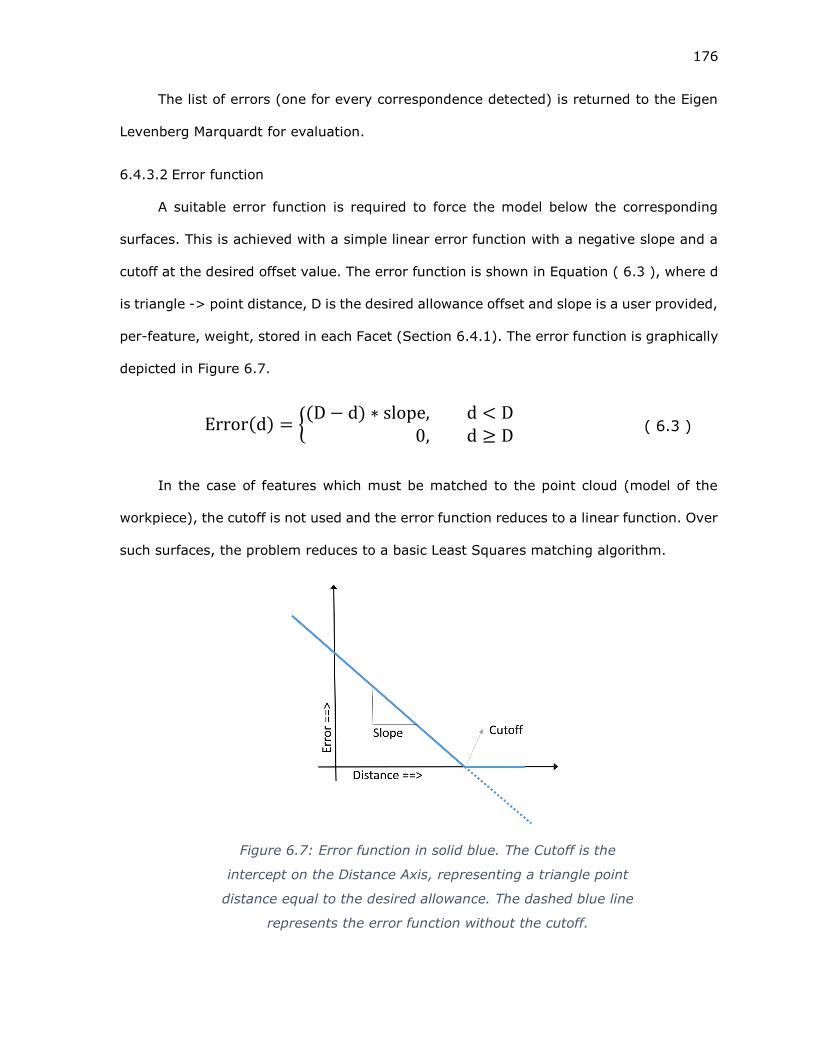
176

The list of errors (one for every correspondence detected) is returned to the Eigen

Levenberg Marquardt for evaluation.

6.4.3.2 Error function

A suitable error function is required to force the model below the corresponding

surfaces. This is achieved with a simple linear error function with a negative slope and a

cutoff at the desired offset value. The error function is shown in Equation ( 6.3 ), where d

is triangle -> point distance, D is the desired allowance offset and slope is a user provided,

per-feature, weight, stored in each Facet (Section 6.4.1). The error function is graphically

depicted in Figure 6.7.

Error(d) = {(D − d) ∗ slope, d < D

0, d ≥ D ( 6.3 )

In the case of features which must be matched to the point cloud (model of the

workpiece), the cutoff is not used and the error function reduces to a linear function. Over

such surfaces, the problem reduces to a basic Least Squares matching algorithm.

Figure 6.7: Error function in solid blue. The Cutoff is the

intercept on the Distance Axis, representing a triangle point

distance equal to the desired allowance. The dashed blue line

represents the error function without the cutoff.

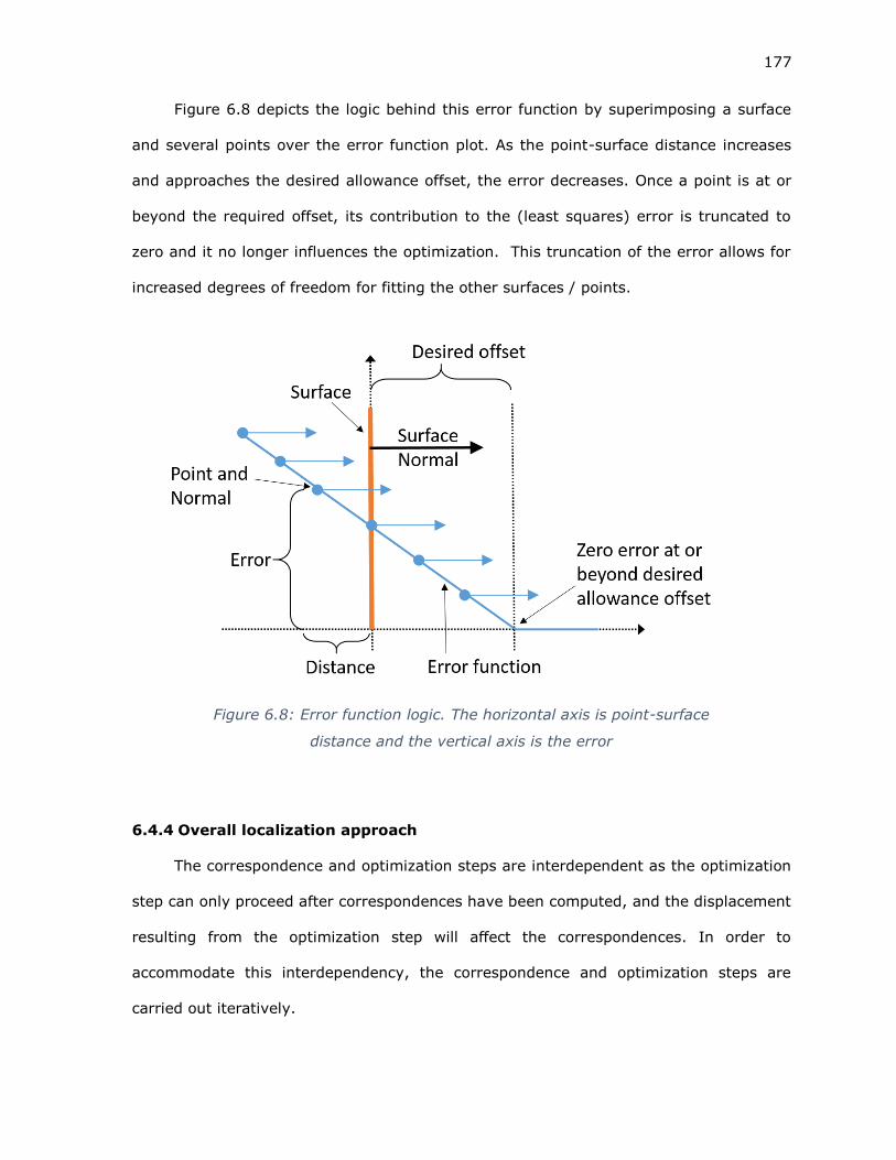
177

Figure 6.8 depicts the logic behind this error function by superimposing a surface

and several points over the error function plot. As the point-surface distance increases

and approaches the desired allowance offset, the error decreases. Once a point is at or

beyond the required offset, its contribution to the (least squares) error is truncated to

zero and it no longer influences the optimization. This truncation of the error allows for

increased degrees of freedom for fitting the other surfaces / points.

6.4.4 Overall localization approach

The correspondence and optimization steps are interdependent as the optimization

step can only proceed after correspondences have been computed, and the displacement

resulting from the optimization step will affect the correspondences. In order to

accommodate this interdependency, the correspondence and optimization steps are

carried out iteratively.

Figure 6.8: Error function logic. The horizontal axis is point-surface

distance and the vertical axis is the error

178

1. The AMF-TOL model and the target point cloud are loaded

2. The list of desired feature weights is accepted from the operator

3. The list of feature allowance offsets is accepted from the operator

4. The ‘Facets’ data structure is generated from the AMF-TOL model

5. The Point cloud is down-sampled

6. The degrees of freedom that the fit must be performed in is accepted from the

operator

7. An initial fit displacement, if provided by the operator is used to displace the model

8. The Point-Facet correspondences are computed

9. The Optimization algorithm is used to fit the model within the material present

10. Steps 8 and 9 are sequentially performed a given number of times, resulting in a

transform that fits the model to the point cloud

179

6.5 Example

The optimization system was integrated into a GUI system for the localization of

models. This user interface is illustrated in Figure 6.9.

For demonstration and visualization, a large initial error was simulated by providing

the system with a large initial error of 0.5 inches (12.7mm) in X and Y as well as an error

of 5 degrees about the X axis.

Figure 6.10 shows the sequence of displacements generated over three iterations of

the procedure. For each iteration, the correspondence estimation took approximately 620

milliseconds and the optimization step between 15 and 31 milliseconds (on a laptop grade

intel m3-6y30 processor). The input data set had 52,019 points after down-sampling with

a grid box size of 0.02 inches. The AMF model had 4,746 triangles. 11 features on the

AMF file were used in the fit. Each of the 11 features has 0.40 inches (1mm) of machining

allowance added prior to additive manufacture. A weight (slope) of ‘5’ was used for each

feature and desired allowance value of 0.03inches (0.762mm) was set for each feature.

Figure 6.9: Best-Fit system UI

180

Subsequent to each iteration the mean offset distance for all point-triangle

correspondence pairs, across each feature, is computed. Figure 6.11 shows these fit

statistics. It can be seen that while most features have adequate allowance, features #4,

#8 and #9 have relatively low machining allowance allocated to them. However, the

allocations are still positive and the overall fit is therefore acceptable.

Figure 6.10: Fit steps. (a) shows initial displacement, (b), (c) and (d) show the

alignment after 1, 2 and 3 iterations respectively

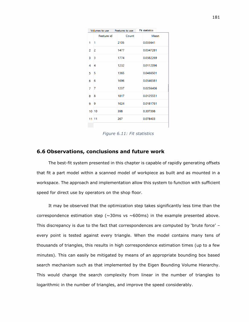
181

6.6 Observations, conclusions and future work

The best-fit system presented in this chapter is capable of rapidly generating offsets

that fit a part model within a scanned model of workpiece as built and as mounted in a

workspace. The approach and implementation allow this system to function with sufficient

speed for direct use by operators on the shop floor.

It may be observed that the optimization step takes significantly less time than the

correspondence estimation step (~30ms vs ~600ms) in the example presented above.

This discrepancy is due to the fact that correspondences are computed by ‘brute force’ –

every point is tested against every triangle. When the model contains many tens of

thousands of triangles, this results in high correspondence estimation times (up to a few

minutes). This can easily be mitigated by means of an appropriate bounding box based

search mechanism such as that implemented by the Eigen Bounding Volume Hierarchy.

This would change the search complexity from linear in the number of triangles to

logarithmic in the number of triangles, and improve the speed considerably.

Figure 6.11: Fit statistics

182

Another challenge is the current lack of a means for automatic determination of the

success of the operation. While statistics are computed, it is left to the operator to interpret

these values and adjust the fit parameters to improve the fit result. The incorporation of

a system that can dynamically analyses the fit statistics and adjust the fit parameters

would provide increased automation and free the operator for other tasks.

183


[1] Z. Li, J. Gou, and Y. Chu, “Geometric algorithms for workpiece localization,” IEEE

Trans. Robot. Autom., vol. 14, no. 6, pp. 864–878, 1998.

[2] A. Gessner, R. Staniek, and T. Bartkowiak, “Computer-aided alignment of castings

and machining optimization,” Proc. Inst. Mech. Eng. Part C J. Mech. Eng. Sci., vol.

229, no. 3, pp. 485–492, Feb. 2015.

[3] A. Gessner, “Patent application nr P-390852 (31.03. 2010),” Method Prep. Cast Iron

Mach. Minimized Mach. Allow.

[4] Y. S. Sysoev, “Positioning, Machining Allowances, and Monitoring the Shape of

Blanks,” Meas. Tech., vol. 44, no. 9, pp. 918–923, Sep. 2001.

[5] J. F. Chatelain and C. Fortin, “A balancing technique for optimal blank part

machining,” Precis. Eng., vol. 25, no. 1, pp. 13–23, Jan. 2001.

[6] J.-F. Chatelain, “A level-based optimization algorithm for complex part localization,”

Precis. Eng., vol. 29, no. 2, pp. 197–207, Apr. 2005.

[7] S. Yuwen, W. Xiaoming, G. Dongming, and L. Jian, “Machining localization and quality

evaluation of parts with sculptured surfaces using SQP method,” Int. J. Adv. Manuf.

Technol., vol. 42, no. 11–12, pp. 1131–1139, Jun. 2009.

[8] G. Tan, L. Zhang, S. Liu, and N. Ye, “An unconstrained approach to blank localization

with allowance assurance for machining complex parts,” Int. J. Adv. Manuf. Technol.,

vol. 73, no. 5–8, pp. 647–658, Jul. 2014.

[9] X. Li, W. Li, H. Jiang, and H. Zhao, “Automatic evaluation of machining allowance of

precision castings based on plane features from 3D point cloud,” Comput. Ind., vol.

64, no. 9, pp. 1129–1137, Dec. 2013.

[10] S. Yuwen, J. Xu, D. Guo, and Z. Jia, “A unified localization approach for machining

allowance optimization of complex curved surfaces,” Precis. Eng., vol. 33, no. 4, pp.

516–523, Oct. 2009.

[11] Y. Dai, S. Chen, N. Kang, and S. Li, “Error calculation for corrective machining with

allowance requirements,” Int. J. Adv. Manuf. Technol., vol. 49, no. 5–8, pp. 635–

641, Nov. 2009.

184

[12] T. Möller and B. Trumbore, “Fast, Minimum Storage Ray/Triangle Intersection,” in

ACM SIGGRAPH 2005 Courses, New York, NY, USA, 2005.


185

Chapter 7

SOFTWARE SYSTEMS

This Chapter contains descriptions of the software systems that contain and utilize

the methodologies described in Chapters 3 through 6.

7.1 AMFCreator

The AMFCreator Graphic User Interface (GUI) software allows an operator to create

and manipulate AMF Files. Functionalities present in AMFCreator include

1. Importing and exporting to and from STL and PLY files

2. Selecting surfaces and associating them with features

3. Adding tolerance information to features

4. Adding machining allowances

5. Computing feature parameters

6. Creating sacrificial support geometry for the DASH process

7.1.1 AMFCreator UI

AMFCreator was written in C++ with the QT [1] widget toolkit and the VTK [2]

visualization system. XML I/O was performed with the TinyXML2 library [3]. The UI

consists of two sections, as seen in Figure 7.1. To the left is a window in which the AMF

model is displayed. Models displayed in this window can be scrolled and panned similar to

any CAD package. The window is also used to demarcate surfaces for association with a

feature, and as a means for selecting volumes and surfaces.

186

To the right of the display window is a list that displays either the set of features or

the set of volumes in the AMF file. The selection is made using radio buttons at the top of

the list. Surface selection controls are present below the list and the feature information

controls, including Metadata is to the right of the list.

7.1.2 Creating an AMF File

A new AMF file can be created by selecting File->Create New AMF in the menus.

Subsequent to this, a new object must be added and then selected as the current object

being worked on. This is performed by selecting the Manage->Add Object menu item.

After the creation of a new object, the object selection UI is automatically launched. The

creation of a new object and its selection is shown in Figure 7.2. AMF files are edited

Figure 7.1: AMFCreator software. Major sections are labeled

187

exclusively in memory. If a file is opened and edited without saving it, no changes will be

preserved. Existing AMF files can be opened and saved via the File menu.

7.1.2.1 Importing tasselated geometry

Once a valid object is selected, tasselated geometry in the form of an ASCII STL or

PLY file may be imported (Binary files are unsupported at this stage) through the Manage

menu. When importing either file type, a threshold distance must be entered by the user.

Any vertices closer than this distance to each other will be combined into a single vertex.

This is necessary when importing STL files as STL duplicates vertices across triangles. The

threshold dialog default value was calibrated to work well across a wide verity of STL/PLY

densities and accuracies. The tasselated geometry is imported as a new volume of the

AMF file. Tasselated geometry imported as an AMF volume is shown in Figure 7.3.

Figure 7.2: Creating and selecting an object

188

The value present in the first metadata element with key equaling “name”, in any

structure, is used as the structure’s name throughout all UI systems.

7.1.3 Creation and management of features

Features may be added to the AMF file by means of the Add button as shown in

Figure 7.4. They may be deleted by selecting a feature in the list and pressing delete.

Figure 7.3: Tasselated geometry imported as volume

Figure 7.4: Adding features

189

When a feature is selected, by clicking on the list item, the feature parameter

controls are enabled. Feature class, id, tolerances and metadata may be added, changed

or removed, as permitted by the AMF-TOL specification. Feature controls are shown in

Figure 7.5. Any metadata associated with a feature is displayed in the Metadata list.

Metadata key value pairs can be edited based on the user’s needs. Metadata elements

may be added by means of the Add button (top right in Figure 7.5) and deleted by using

the delete (‘X’) button attached to each metadata item.

Once a feature’s data has been edited, it must be associated with the feature by

clicking the ‘Set’ button, as shown in Figure 7.4. If another feature is selected before ‘Set’

is clicked, all changes and edits will be lost. In addition, when a feature is selected, all

triangles associated with it are highlighted in the display window.

Figure 7.5: Feature controls

190

7.1.4 Triangle selection

Surfaces are selected by clicking on them in the AMF display. The selection controls

determine the extents of the selection. In AMFCreator, surface selection is performed

based on a region-growing algorithm. The first triangle clicked on is always selected.

Triangles that neighbor this triangle are selected if their angles (comparing triangle

normals) are within a specified threshold. Following this, the triangles that now neighbor

the newly selected triangles, i.e. on the edges of the selected region, are tested and

selected. The set of selected triangles is continuously grown until no more triangles are

available to test and select.

The angle threshold may be specified as either a relative threshold or as an absolute

value, by selecting the absolute checkbox. When relative (non-absolute) thresholding is

used, each triangle on the edge of the selected region is selected if its angle with respect

to one of its already selected neighbors is within the selection threshold. If an absolute

threshold is used, each triangle on the edge is tested against the first triangle that was

selected. If the deselect box is checked, triangles that meet the threshold criteria are de-

selected instead. The clear button can be used to deselect all triangles.

Figure 7.6: Selection parameter controls

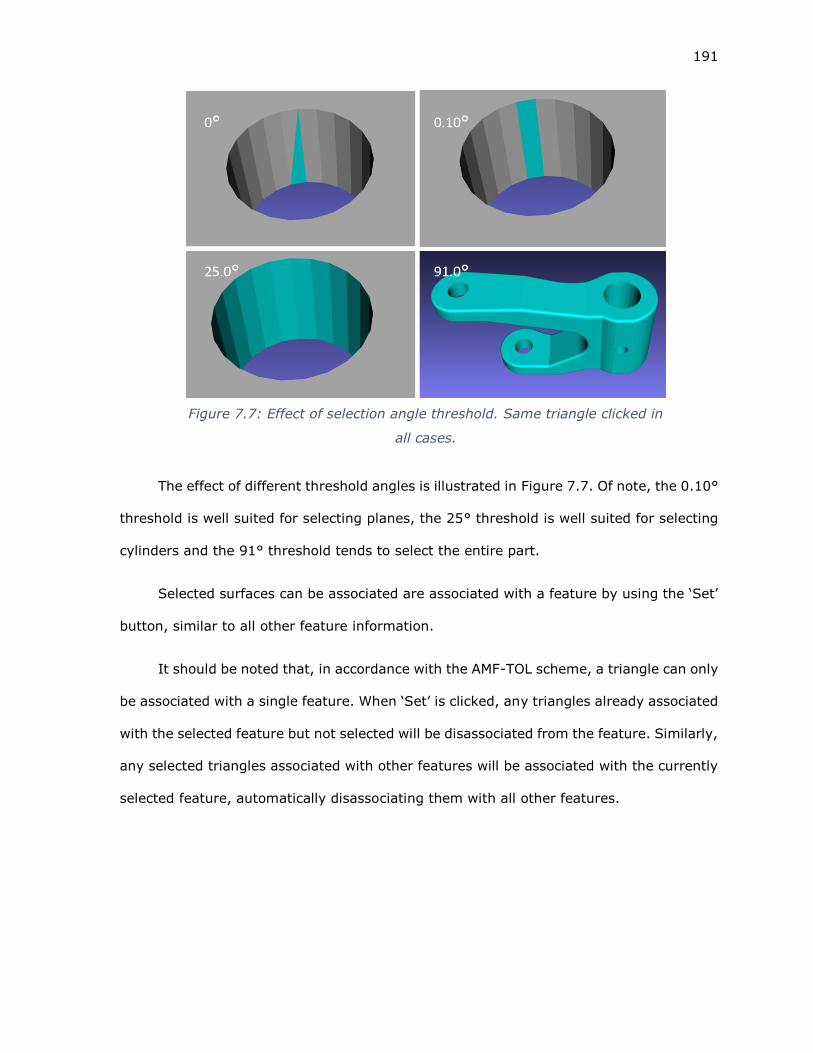
191

The effect of different threshold angles is illustrated in Figure 7.7. Of note, the 0.10°

threshold is well suited for selecting planes, the 25° threshold is well suited for selecting

cylinders and the 91° threshold tends to select the entire part.

Selected surfaces can be associated are associated with a feature by using the ‘Set’

button, similar to all other feature information.

It should be noted that, in accordance with the AMF-TOL scheme, a triangle can only

be associated with a single feature. When ‘Set’ is clicked, any triangles already associated

with the selected feature but not selected will be disassociated from the feature. Similarly,

any selected triangles associated with other features will be associated with the currently

selected feature, automatically disassociating them with all other features.

Figure 7.7: Effect of selection angle threshold. Same triangle clicked in

all cases.

192

7.1.5 Volume management

Volumes of the AMF file are managed similarly to features. The volumes of the AMF

file may be managed by selecting the ‘Volumes’ aspect radio button. Selecting a volume

in the list highlights the volume in the display window, as seen in Figure 7.8. The set of

visible volumes may be changed by means of the View->Select Volumes menu item. This

displays the select volumes dialog, shown in Figure 7.9 AMFCreator is capable of

intelligently removing vertices when volumes are deleted - all vertices that are referred

to be triangles in the volume, but not by triangles in other volumes are deleted along with

the volume. All other vertices are preserved.

Figure 7.8: Volume management. Seen is volume list with selected

volume. Selected volume highlighted in the display window.

Figure 7.9: Volume visibility dialog box.

193

7.1.6 Computation of feature parameters

Feature parameters include parameters of Size, Orientation, and position.

AMFCreator includes methods for the computation of parameters for plane and cylinder

features. Parameters are computed through the DASH->Compute Parameters menu item.

This triggers parameter computation for all features in the AMF file.

7.1.6.1 Plane features

For a feature marked as a plane, the feature parameter extraction routine extracts

the plane centroid and normal. The centroid is computed as the area-weighted centroid of

all triangles comprising the plane. The plane normal is, similarly, the area-weighted

average normal of all triangle normals comprising the plane.

7.1.6.2 Cylinder features

For a cylinder feature, a least squares fit (using the Eigen library’s Levenberg

Marquardt algorithm [4]) is performed to estimate the cylinder parameters. Triangle

vertices and centroids are both used to perform the best fit, in order to compute the best

fit cylinder rather than the circumscribing cylinder. Once the cylinder parameters have

been extracted (axis point, axis direction and diameter). The ‘top’ and ‘bottom’ of the

cylinder are computed by projecting all cylinder points onto the axis.

In addition to the cylinder parameters, the parameter system also checks if a

cylinder is a hole or a boss and checks if a hole cylinder is ‘blind’ or ‘through’. The ‘top’

and ‘bottom’ positions are flipped, if necessary, to make them consistent with a blind hole.

Computed parameters are stored as feature metadata, illustrated in Figure 7.10

194

7.1.7 Addition of machining allowances

Machining allowance can be added to a part through the DASH->Add Machining

Allowance menu item. This triggers a dialog for addition of machining allowances, shown

Figure 7.10: Cylinder feature and extracted parameters. Parameters

displayed as metadata

Figure 7.11: Addition of machining allowances. Resulting allowance highlighted in

display window.

195

in Figure 7.11. The allowance dialog allows a user to add and select the set of features to

add machining allowance to and how much allowance to add. The ‘overall’ item allows

machining allowance to be added to non-feature surfaces. Chapter 4 contains a complete

description of the machining allowance generation system.

Machining allowances are added to a part as a separate volume. The parameters

used to generate the machining allowance are added to the volume as metadata.

7.1.8 Creation of sacrificial support geometry

The DASH Sacrificial support geometry consists of two fixturing features each

attached to the part by two struts. The part must be moved to its manufacturing pose

before the support geometry is added. The full procedure is as follows:

Load transformation and sacrificial support information

1. Transform the AMF file by the provided transform

2. Create and add four struts

3. Load the geometry for the support structure

4. Stretch the geometry for the support structure to encompass the struts

5. Mirror add a second support structure at the other end of the part

This sequence is illustrated in Figure 7.12

196

Support generation is triggered by selecting the DASH->Transform+Supports Menu

Item. This displays the support generation UI, shown in Figure 7.13.

To the left and right of the support UI are fields where a user can enter the strut

parameters – position, length and diameter. The Center of the UI contains 12 input fields

where the user can provide a transformation matrix. Also in the central column are inputs

for a user to enter a quaternion transform (angle and axis) that can be used to populate

the transformation matrix by using the ‘Set’ button. Strut and transform information can

be loaded from DASH XML files by means of the ‘Load Struts XML’ and the ‘Load Transform

XML buttons’, respectively. Once all parameters have been entered, the Transform +

generate button is used to perform the sequence of operations.

Figure 7.12: Support geometry generation stages. (a) is initial geometry (b)

transformation to manufacturing position (c) support struts (d) fixturing features

197

7.1.8.1 Transformation

The transformation of the AMF geometry is achieved by applying the transformation

matrix to each vertex

7.1.8.2 Struts

The struts are each generated by creating 8 vertices and 12 triangles to form a strut

with a square cross section. The diameter parameter is used for the diagonal of the cross

section. Struts are saved as a separate volume.

7.1.8.3 Fixturing features

The Support Generation expects the user to open a specially prepared AMF file

holding the support geometry. The AMF file must be the ‘right side support’ positioned

with the strut attachment surface plane coincident with the YZ plane and the ‘disk edge’

must be demarcated as a feature with id #1. In addition, the support file must be saved

in mm units. Left and right are as seen in Figure 7.12.

Subsequent to selecting an AMF file containing the support geometry, the system

queries the user on the initial diameter of the disk (always in mm) and based on the strut

Figure 7.13: Support Generation UI

198

positions and diameters, suggests a stretched size for the disk (in file units). Two sacrificial

support structures are added to the part. The ‘left side support’ is generated by rotating

the ‘right side support’ 180° about the Y axis. The supports are added at the extents of

the part + struts. i.e. The right side support is added at the maximum X and the left side

at the minimum X. Figure 7.12 illustrates the stages of support generation.

7.2 SCANUI

The SCANUI software package includes routines for scan management, interfacing

with the HAAS VF3 and implementations of the registration and localization systems. The

SCANUI user interface is shown in Figure 7.14. Similar to AMFCreator, SCANUI was written

with the QT toolkit and the VTK display library. The left side of the SCANUI interface is

dominated by a display window. To the right of the display window is a list of the point

clouds that are currently open/loaded. To the right of this list are tabs that switch between

the scan management, registration and localization controls.

Figure 7.14: SCANUI interface elements

199

7.2.1 Scan management

SCANUI assigns a unique number to each point cloud. Selecting a cloud causes it to

be rendered in the display window. In addition, SCANUI can perform several scan-

management functions.

Most operations in SCANUI are asynchronous. As computations are performed, the

user may continue to perform other tasks. Thread synchronous checks are used to ensure

that the user cannot accidentally invalidate data. For example, by deleting a scan while it

is still being loaded.

7.2.1.1 Loading and Saving files

Scans can be saved as ASCII ‘.xyz’ or ‘.asc’ files by selecting a scan and clicking

save. Scans are loaded by clicking the ‘Load Files’ button. Multiple files may be selected

when loading scans.

7.2.1.2 Clipping scans

Scans may be clipped along the X axis. As seen in Figure 7.14, two clip planes are

displayed in the display window. When the Clip Scan button is clicked, all points between

the two clip planes are copied into a new point cloud. This is shown in Figure 7.15

The clip planes can be positioned or hidden using controls in the display management

section of the SCNUI interface.

Figure 7.15: Point cloud on right created by clipping the point cloud on the left

200

7.2.1.3 Down-sampling scans

As described in Chapter 6, down-sampling is required to produce a noise-free point

cloud with even spacing for the localization algorithm. Down-sampled point clouds are also

required for reconstruction of a mesh model. Figure 7.16 shows the down-sampling

process. The cloud to the left contained 39661 points and was down-sampled with a box

size of 0.05 inches and a filter threshold of 4 points per box resulting in a scan with 4006

points, on the right. Down-Sampling is triggered by selecting the scan in the scan list and

clicking the Down-Sample Button.

7.2.1.4 Creating a mesh model

Mesh models can be created from a point cloud by using the ‘Make Stock Model’

button. The stock models are created using the Poisson Surface Reconstruction [5] routine

in the PCL [6] library. This is illustrated in Figure 7.18. The point cloud on the left was

meshed to create the STL model on the right. The mesh creation system in SCANUI

includes the ability to overgrow (increase the size) of a mesh by offsetting all points along

their normal directions.

Figure 7.16: Down-sampling of scans

201

7.2.2 Interface with FARO scanner

The SCANUI software can fetch point clouds directly from a FARO Edge Arm + Laser

scanner. This is accomplished by connecting the FARO Arm to the PC, on which SCANUI

is running, via USB and opening a new connection by means of the ‘Refresh Connection’

button in the ‘Faro scanner control’ group. The ‘Refresh Connection’ button will indicate if

a connection was successfully made and will report if the connection was lost. When an

active connection is present, a new scan can be triggered by pressing the ‘New Scan’

button.

Figure 7.18: Meshing of point cloud

Figure 7.17: Faro scanner control options

202

When scanning, the scan may be paused/resumed with button #1 (Green) on the

FARO scanner and stopped with button #2 (Red). Scanning may also be stopped by

pressing the ‘New Scan’ button. The text of this button is changed to ‘SCANNING – Press

to Stop’ to reflect this. By default, data is gathered in inch units. The ‘Use Millimeters’

checkbox can be used to collect data in millimeters. The ‘Enable Reference Dialog’

checkbox enables and disables the FARO Reference Dialog and the ‘Scanner Settings’ and

‘Faro Hardware Config’ buttons open the corresponding dialogs from the FARO software

drivers.

When Scanning, enabling the ‘Track arm position’ checkbox causes the display to

track a virtual camera ‘attached’ to the scanning head on the FARO Arm. When disabled,

the display must be moved and positioned manually. As the scanner collects points, the

display is updated to display the newly acquired points. The ‘Display Refresh Multiplier’

value controls the fractional rate at which the display is refreshed relative to the scanning

rate. For example, a value of 5 causes the display to refresh every 5 ‘sets’ of points taken

by the scanner.

7.2.2.1 Computation of normals

Since many algorithms described in this Dissertation require point normal

information, point normals must be computed when scanning is completed. Computation

of normals is initiated automatically, when scanning is stopped.

Figure 7.19: Approximate point normal

203

Point normal computation is performed in two stages. When the scan is being taken,

point normals are set to a vector aligned along the negative of the scanner view vector at

the instant the point was captured. This is illustrated in Figure 7.19.

When scanning is completed, a grid data structure, similar to the grid used in down-

sampling, is used to extract the neighbors of a point within a specified distance (specified

in the ‘Normal Computation Radius’ control). Singular Vector Decomposition is performed

on the positions of these neighbors and the third largest singular vector is used as the

normal at that point. If the ‘Reject Bad Normals’ checkbox is selected, all points with fewer

than 9 other points within the specified radius, or with a computed normal more than 45°

away from the approximate point normal are deleted from the scan.

7.2.3 Interface with CNC Machine

The Registration system, described in Chapter 5, requires the transform from the

machine position at which the datums were detected and the machine position at which

each part scan is taken. To do this, the alpha position of the rotary axis must be recorded

as each scan is taken.

While the angle may be recorded manually, SCANUI includes a system for direct

retrieval of machine position information from the HAAS, over a serial port. To retrieve

the current position of the rotary axis, two values must be read from the HAAS – the axis

position in ‘machine coordinates’ and the current value of the work offset. The axis position

in the work offset is computed by subtracting the work offset from the machine position.

The SCANUI serial port interface includes input fields where the appropriate

variables, COM port and Baud Rate may be specified. If the ‘Fetch position’ box is checked,

the Position and Offset values are fetched from the HAAS whenever a new scan is started.

The computed axis position is associated with the scan.

204

7.2.4 Registration

Registration of scans (Chapter 5) in SCANUI is performed in a two stage process –

computing the transform and stitching scans together. An operator must scan the chuck

and take as many scans of the part as required. If the Serial Port system is not used to

automatically detect the chuck axis position at each scan, the operator must record these

values. Care must be taken to keep the positions of the scanner and CNC machine fixed

throughout the scanning process.

7.2.4.1 Computing transforms

The registration transform is computed by selecting a scan of a chuck, and extracting

the chuck datums as descried in Chapter 5. The datum extraction parameters can be

entered in the input fields, shown in the top half of Figure 7.21. The ‘Faces -veX?’ check

box is used to inform the system that the fiducial chuck faces the negative X direction.

The ‘Angle at scan’ parameter is used to inform the system if the chuck was scanned at a

rotation angle other than 0°. If the serial port system is enabled, this parameter is

populated automatically. The ‘Chuck Face Offset’ field is used to specify the offset, along

the chuck axis of the chuck face from the work offset coordinate system. All other

parameters are as described in Chapter 5.

Figure 7.20: Serial port controls

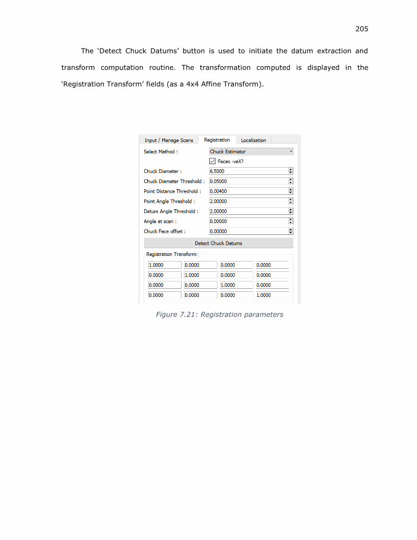
205

The ‘Detect Chuck Datums’ button is used to initiate the datum extraction and

transform computation routine. The transformation computed is displayed in the

‘Registration Transform’ fields (as a 4x4 Affine Transform).

Figure 7.21: Registration parameters

206

7.2.4.2 Model Reconstruction

Figure 7.22 shows the system for stitching scans together. The ‘Add scan to list’

button is used to add rows to the list. The ‘X’ button can be used to remove rows. Each

row contains a dropdown list that can be used to select scans by unique id. Each row also

contains an input field for the chuck axis angle at which a scan was taken. If the serial

port system is used, the chuck axis angle values are populated automatically. Figure 7.22

also shows the computed registration transform.

Figure 7.22: Stitching scans together. Shown are the combined extracted datums

and four scans to be stitched together.

207

When the ‘Register Selected Scans’ button is pressed, the computed transform and

angle information is used to stitch the selected scans into a combined model. Figure 7.23

shows the combined, registered scan resulting from the parameters and selections shown

in Figure 7.22.

7.2.5 Localization

The localization system is described in Chapter 6. The following systems describe

the implementation of this methodology in SCANUI.

7.2.5.1 Loading a part model

In DASH, part models are represented as toleranced AMF files (AMF-TOL). In

SCANUI, an AMF-TOL file is loaded by means of the ‘Load AMF’ button in the Localization

Tab. When an AMF file is loaded, the user is presented with a dialog for selecting the AMF

object (by id). To display the AMF, the ‘Display AMF’ checkbox must be selected along

with the desired volumes, in the ‘Volumes to use’ section. This is shown in Figure 7.24.

Figure 7.23: Combined, registered scan

208

7.2.5.2 Features and feature parameters

The set of features against which localization is performed can be selected in the

‘Features to use’ tab within the ‘Localization’ tab. The ‘Features to use’ tab is shown in

Figure 7.26. The list of features is automatically populated from the AMF file. Each row in

the list represents a single feature. Features are identified by id and the value of a ‘name’

metadata field, if present.

Figure 7.24: Localization controls

209

Each row also has fields for setting the ‘weight’ and offset (see Chapter 6) that is

used for each feature. A checkbox to the right of each row can be used by the operator to

indicate if the feature should be used or not. Any features for which machining allowances

have been added, are automatically selected and the machining allowance offset value is

used to populate the ‘Offset’ field. The corresponding surfaces of a selected feature are

highlighted in the display window, illustrated in Figure 7.25.

Figure 7.26: Features to use

Figure 7.25: Model with selected features highlighted

210

7.2.5.3 Localization

The offsets group, also shown in Figure 7.24 has fields for the model displacement.

These fields can be populated by the operator and are updated automatically by the

Localization system. When the ‘Transform Displayed AMF’ Checkbox is selected, the offset

values are applied to the displayed AMF model. When the offset fields are updated by the

software, a model position update is automatically triggered. If they are updated by the

operator, the ‘Transform Displayed AMF’ must be toggled to trigger a model update. The

‘Angle Cutoff’ and ‘Distance Cutoff’ fields allow the operator to specify the correspondence

estimation threshold values, as specified in Chapter 6.

7.2.5.4 Statistics

Based on the correspondence system described in Chapter 6, the mean and variance

of the point-surface distances over each feature is computed and updated in the ‘Fit

Statistics’ tab as shown in Figure 7.27. These values help the operator to assess the quality

of the fit.

Figure 7.27: Fit and associated statistics

211

7.3 Conclusions

This Chapter provides descriptions of the software systems that incorporate the

methodologies developed in Chapters 3 through 6. AMFCreator and SCANUI enable an

operator to:

1. Create a toleranced AMF file (AMF-TOL)

2. Automatically Add machining allowances

3. Add sacrificial supports

4. Scan a part in a CNC machine

5. Register scans, to create an as built and as it is mounted model of a workpiece

6. Automatically determine the offsets at which to harvest a part from the material

present

212


[1] “Qt - Home,” Qt. [Online]. Available: https://www.qt.io/. [Accessed: 24-Apr-2016].

[2] “VTK - The Visualization Toolkit.” .

[3] “TinyXML-2.” [Online]. Available: http://www.grinninglizard.com/tinyxml2/.



[5] M. Kazhdan, M. Bolitho, and H. Hoppe, “Poisson surface reconstruction,” in

Proceedings of the fourth Eurographics symposium on Geometry processing, 2006,

vol. 7.

[6] R. B. Rusu and S. Cousins, “3d is here: Point cloud library (pcl),” in Robotics and

Automation (ICRA), 2011 IEEE International Conference on, 2011, pp. 1–4.

213

Chapter 8

SUMMARY AND FUTURE WORK

This chapter contains a broad summary of the systems and methodologies

developed in this dissertation. As specific conclusions and avenues for future work are

included in the chapters dedicated to each of these systems, this chapter focusses on

assessing these systems as a whole, rather than as individual components.

The DASH system was developed as a means for the rapid production of a part that

meets the required tolerance specifications from a digital model. In order to achieve this,

four components, required by the DASH process, were developed in this dissertation.

1. A file format which includes Product and Manufacturing Information (PMI) in the

form of the AMF-TOL format

2. A system for the automated, feature based, addition of machining offsets

3. An in-process sensing system capable of automatically detecting datum surfaces

and constructing a part model as built and as it is mounted in a CNC machine

4. A system for automatically computing machining offsets for harvesting a part from

a workpiece geometry model

AMF-TOL represents a bottom-up approach towards integrating PMI into a geometry

model and thereby creating a Model Based Definition (MBD) that can drive the many

stages of the DASH process. Compared to formats such as STEP, AMF-TOL’s primary

advantages are flexibility, simplicity and extensibility, though this comes at the lack of

support for exact geometry.

214

MBD is required for both process planning and geometry modification. The DASH

process incorporates two geometry modification systems – machining allowance

generation and sacrificial support addition. The machining allowance generation system,

presented in Chapter 4, creates machining allowance ‘volumes’ by offsetting the vertices

of the AMF mesh structure. While several prior works utilized vertex displacement methods

for mesh offset, their approaches suffered from deficiencies in the solution method for the

offset vector. This was addressed by the development of an optimization based approach

for displacement vector computation.

In current practice, fixture planning is a time consuming and expensive process.

DASH addresses this by incorporating standardized fixturing features into the part

geometry prior to the production of the near-net-shape workpiece in an AM system. The

PMI information, as encapsulated in the AMF-TOL MBD is used to plan the position and

orientation of these fixturing features and they are generated directly in the AMF-TOL

mesh model.

Part localization, the act of determining the position at which a part must be

machined, is another aspect of modern manufacturing practice that is time consuming and

expensive. Chapters 5 and 6 contain a novel methodology for automatic part localization

to address this in the DASH system. In Chapter 5, a system that can automatically register

3D scans to a workspace coordinate system, by detecting fiducial features in scan data,

was developed. This system can generate a model of the workpiece as built and as it is

mounted in a CNC machine. This is invaluable to process planning. In Chapter 6, a system

for generating offsets that move the part model, from its nominal pose ‘into’ the workpiece

material was presented. At the offset pose, the model may be ‘harvested’ from the

workpiece material by finish machining. This localization system, again relies on the MBD

provided by the AMF-TOL file.

215

DASH functions by following a fixed formula for the production of parts. Rather than

modifying the process to suit a part, the part is modified to suit the process. This imposes

some limitations on the geometries that may be produced, largely as a product of the

fixturing and finishing strategy employed (fixturing between centers and island / waterline

milling, respectively). Geometries such as mesh structures and internal channels cannot

be finish machined by DASH (or by any other conventional machining strategy).

Despite this lack of generality, DASH is a concrete implementation of an automated

digital manufacturing system. The subsystems of DASH embody nearly all aspects of the

digital manufacturing system - MBD, automatic geometry modification, automatic process

planning and in-machine sensing. These components can be composed and extended to

incorporate more aspects of a complete part production system, and thereby improve the

ability of DASH to add value.

Many parts require grinding and other post-finishing operations in order to meet

the tolerances required of them. In the DASH process, in its current form, a model of the

part which includes grinding allowances must be created manually. A future version of the

DASH process may include a hierarchy of features and machining allowances. Each level

in the hierarchy represents the target of an upstream process and the expected (nominal)

stock model for a downstream process. This would enable, for example, a system in which

finish machining must be followed by grinding and honing.

As the DASH process already includes a part model with features and tolerances,

together with an in-process sensing system, including in-process inspection is a feasible

and valuable future goal. A scan of the part after completion of each finishing operation

can be used to determine if a part is within specification. If the finished geometry falls

outside the acceptable range, a rework strategy may be formulated. If no rework strategy

is viable, the part can be rejected early, before further time and resources are wasted.

216

The proposed grinding and inspection systems leverage the AMF-TOL MBD. This can

be further leveraged by incorporating the models and other data generated by in-machine

sensing systems into the AMF-TOL. Such a file would include the as-produced (and

measured) geometry together with the desired geometry at each stage of the hierarchical

production process, and would form a digital twin, of the part. This would prove invaluable

for tractability, inspection and analysis.

etd.pdf - NCSU Repository

Documents