Estudio de las propiedades fractales de árboles …paguirre.mat.utfsm.cl/mat288-2016-1/PresentacionRoger.pdf · Estudio de las propiedades fractales de árboles eléctricos y de

Estudio de las propiedades fractales de árboles eléctricos y de la dinámica de las descargas parciales involucradas

en la degradación de aislamientos eléctricos

1

Roger SchurchDepartamento de Ingeniería Eléctrica

Presentación (adaptada) para asignatura Laboratorio de Modelación MAT-2884 de abril de 2016

TEMA 1

Propiedades fractales de árboles eléctricos

2

Overview

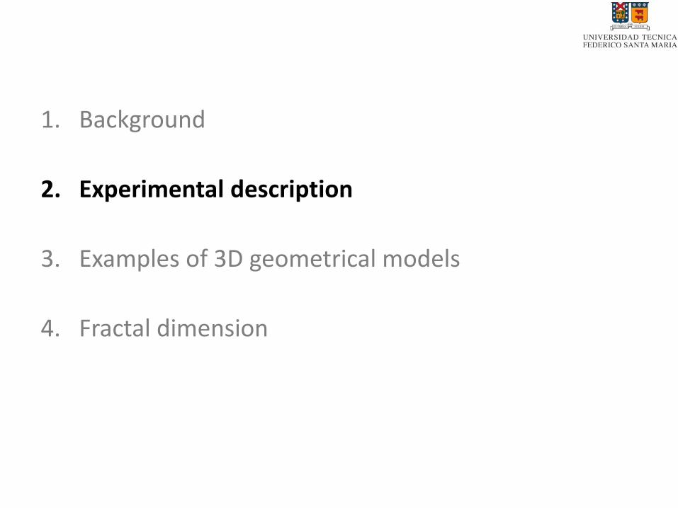
1. Background

2. Experimental description

3. Examples of 3D geometrical models

4. Fractal dimension

1. Background

2. Experimental description

3. Examples of 3D geometrical models

4. Fractal dimension

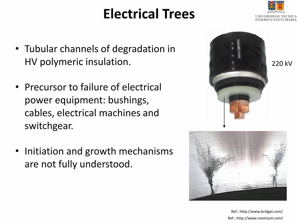
Electrical Trees

• Tubular channels of degradation in HV polymeric insulation.

• Precursor to failure of electrical power equipment: bushings, cables, electrical machines and switchgear.

• Initiation and growth mechanisms are not fully understood.

220 kV

Ref.: http://www.bridgat.com/

Ref.: http://www.novinium.com/

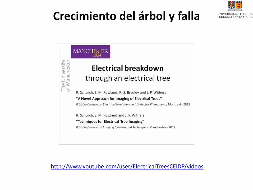
Crecimiento del árbol y falla

http://www.youtube.com/user/ElectricalTreesCEIDP/videos

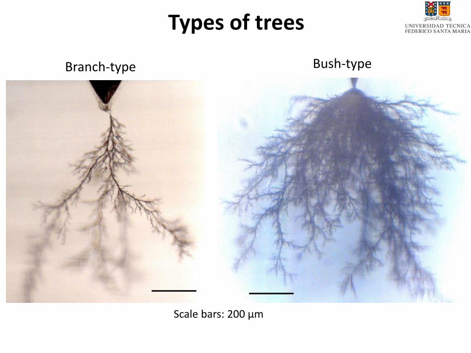
Types of trees

Scale bars: 200 µm

Branch-type Bush-type

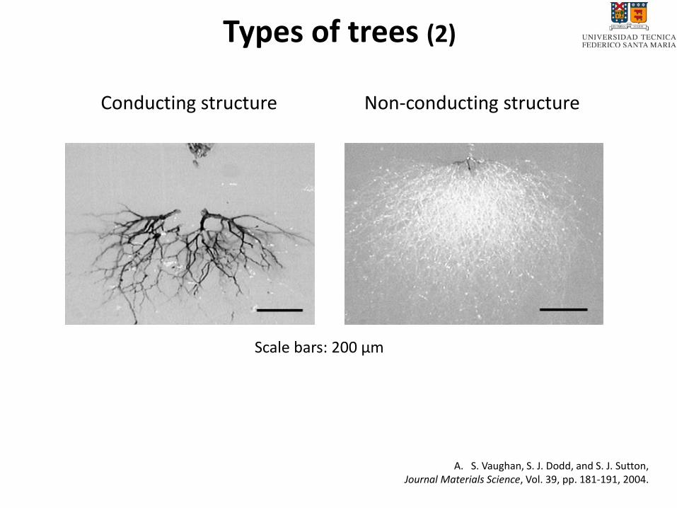
Types of trees (2)

A. S. Vaughan, S. J. Dodd, and S. J. Sutton,Journal Materials Science, Vol. 39, pp. 181-191, 2004.

Conducting structure

Scale bars: 200 µm

Non-conducting structure

Importance of studying Electrical Trees

• Study the mechanisms involved in the phenomena

• Lead to improved insulation design and asset management

→ increase reliability of power networks

→ achieve challenges of new requirements of plant compaction and energy loss reduction

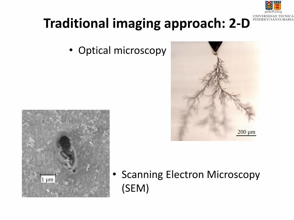
Traditional imaging approach: 2-D

• Optical microscopy

• Scanning Electron Microscopy (SEM)

200 µm

1 µm

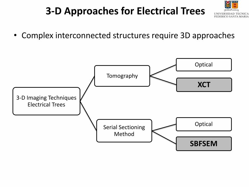
3-D Approaches for Electrical Trees

3-D Imaging Techniques Electrical Trees

Serial Sectioning Method

Optical

SBFSEM

Tomography

Optical

XCT

• Complex interconnected structures require 3D approaches

1. Background

2. Experimental description

3. Examples of 3D geometrical models

4. Fractal dimension

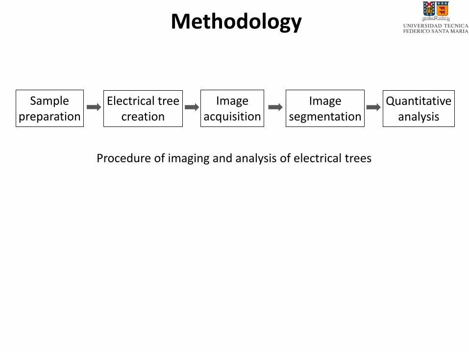
Methodology

Samplepreparation

Electrical treecreation

Imageacquisition

Imagesegmentation

Quantitativeanalysis

Procedure of imaging and analysis of electrical trees

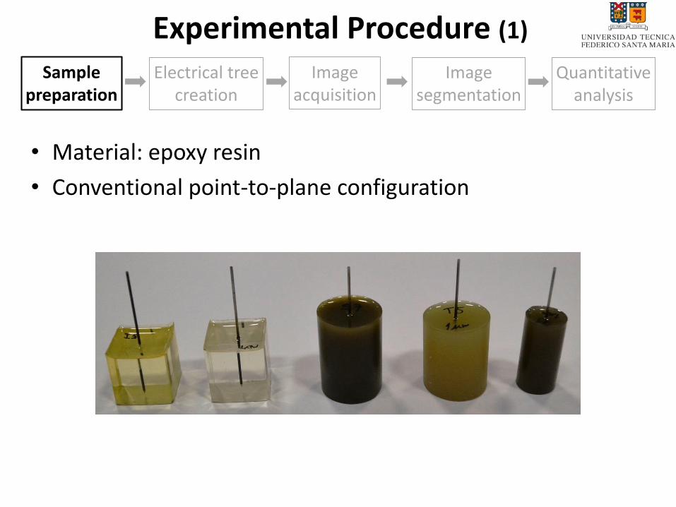
Experimental Procedure (1)

Samplepreparation

Electrical treecreation

Imageacquisition

Imagesegmentation

Quantitativeanalysis

• Material: epoxy resin

• Conventional point-to-plane configuration

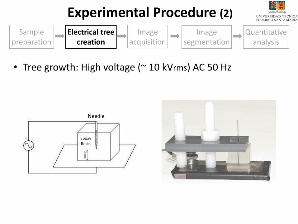
Experimental Procedure (2)

Samplepreparation

Electrical treecreation

Imageacquisition

Imagesegmentation

Quantitativeanalysis

Needle

EpoxyResin

• Tree growth: High voltage (~ 10 kVrms) AC 50 Hz

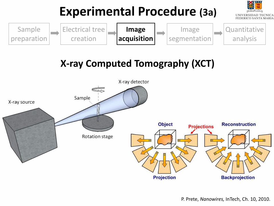
Experimental Procedure (3a)

Samplepreparation

Electrical treecreation

Imageacquisition

Imagesegmentation

Quantitativeanalysis

P. Prete, Nanowires, InTech, Ch. 10, 2010.

X-ray Computed Tomography (XCT)

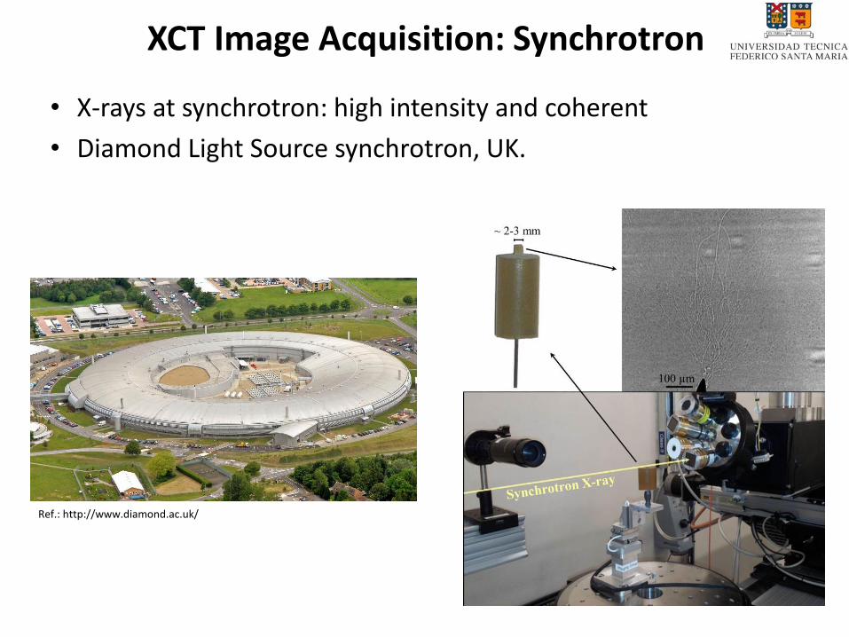
XCT Image Acquisition: Synchrotron

• X-rays at synchrotron: high intensity and coherent

• Diamond Light Source synchrotron, UK.

Ref.: http://www.diamond.ac.uk/

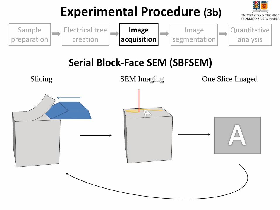
Experimental Procedure (3b)

Samplepreparation

Electrical treecreation

Imageacquisition

Imagesegmentation

Quantitativeanalysis

Serial Block-Face SEM (SBFSEM)

Slicing SEM Imaging One Slice Imaged

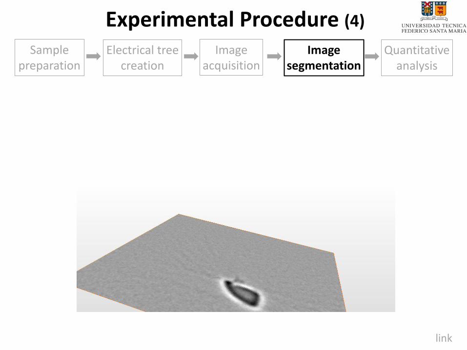
Experimental Procedure (4)

Samplepreparation

Electrical treecreation

Imageacquisition

Imagesegmentation

Quantitativeanalysis

link

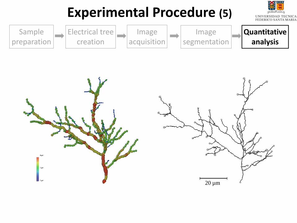
Experimental Procedure (5)

Samplepreparation

Electrical treecreation

Imageacquisition

Imagesegmentation

Quantitativeanalysis

20 µm

1. Background

2. Experimental description

3. Examples of 3D geometrical models

4. Fractal dimension

Algunos ejemplos de la data disponible

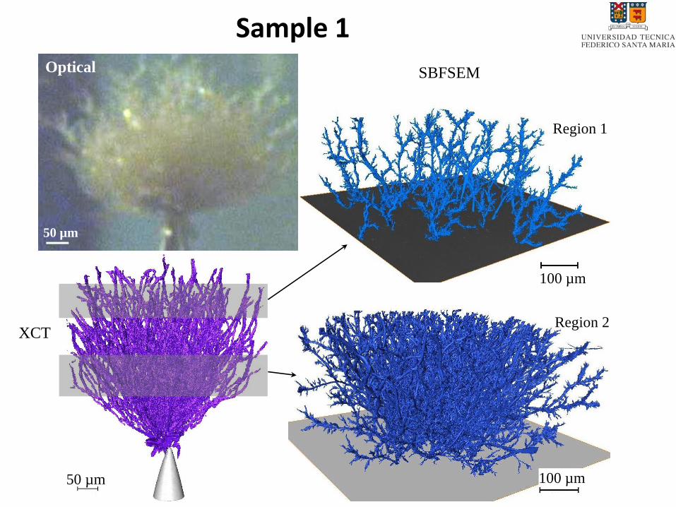
Sample 1

XCT

SBFSEMOptical

50 µm

Region 1

Region 2

50 µm

100 µm

100 µm

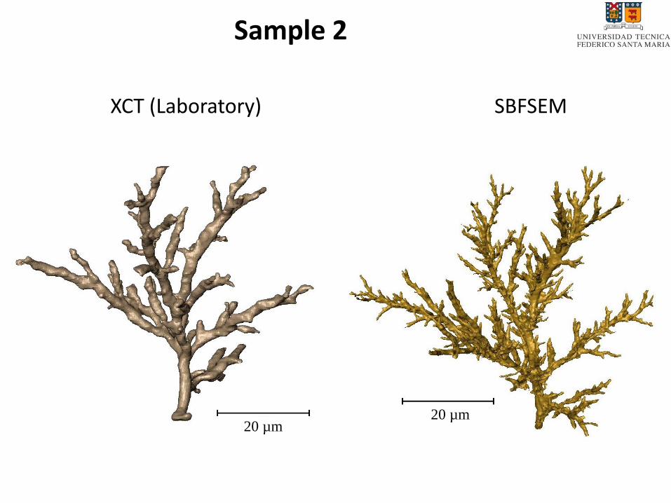
XCT (Laboratory) SBFSEM

20 µm20 µm

Sample 2

link

Sample 3 (animation)

La data disponible es una pila de imágenes 2D ya segmentadas

1. Background

2. Experimental description

3. 3D geometrical model creation

4. Fractal dimension

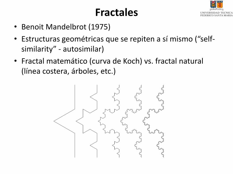
Fractales• Benoit Mandelbrot (1975)

• Estructuras geométricas que se repiten a sí mismo (“self-similarity” - autosimilar)

• Fractal matemático (curva de Koch) vs. fractal natural (línea costera, árboles, etc.)

Árboles eléctricos y dimensión fractal

• Árboles eléctricos poseen estructura compleja que noes posible de describir analíticamente.

• La forma de los árboles eléctricos se describe a través de su dimensión fractal.

• Algunos modelos matemáticos de crecimiento de árboles eléctricos utilizan la dimensión fractal como uno de sus parámetros fundamentales.

• Árboles de dimensión fractal más pequeña crecen más rápido (son más peligrosos)

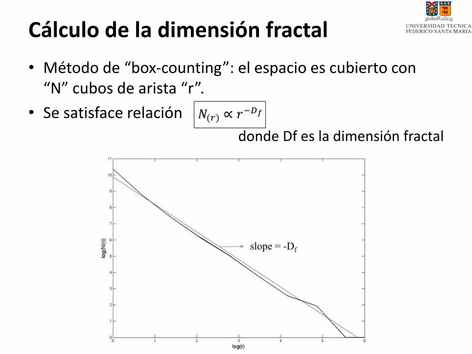
Cálculo de la dimensión fractal

• Método de “box-counting”: el espacio es cubierto con “N” cubos de arista “r”.

• Se satisface relación

donde Df es la dimensión fractal

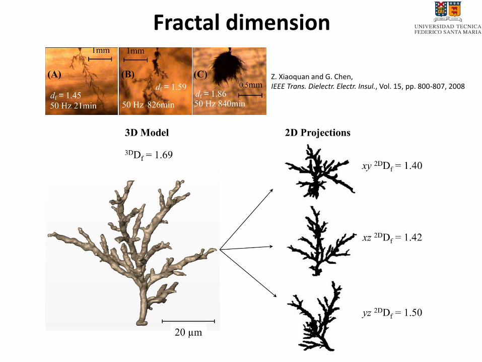
Fractal dimension

Z. Xiaoquan and G. Chen, IEEE Trans. Dielectr. Electr. Insul., Vol. 15, pp. 800-807, 2008

Algunas preguntas a investigar

• ¿Son los árboles eléctricos estructuras que podemos categorizar como fractales?

• ¿Es la dimensión fractal el mejor parámetro que caracteriza la forma de un árbol eléctrico?

• ¿Cuál es el mejor método para la estimación de la dimensión fractal en árboles eléctricos?

• ¿Cuál es la relación entre la dimensión fractal estimada desde una imagen 2D y la del objeto real 3D?

• ¿En qué error estaban incurriendo los investigadores al estimarla desde imágenes proyectadas 2D?

Extra:Caracterización

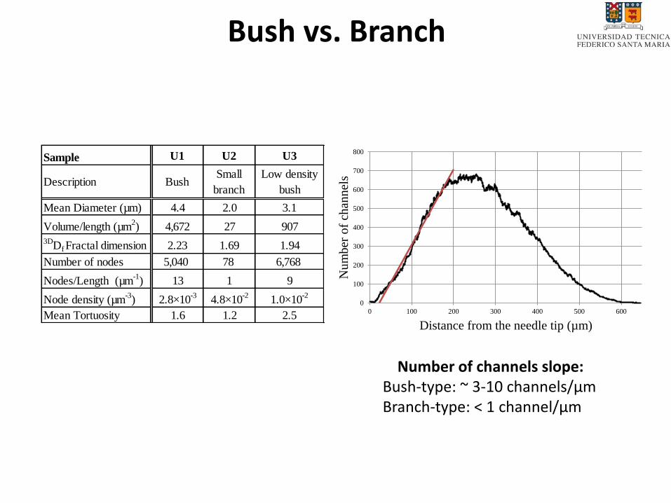
Bush vs. Branch

Sample U1 U2 U3

Description BushSmall

branch

Low density

bush

Mean Diameter (µm) 4.4 2.0 3.1

Volume/length (µm2) 4,672 27 907

3DDf Fractal dimension 2.23 1.69 1.94

Number of nodes 5,040 78 6,768

Nodes/Length (µm-1

) 13 1 9

Node density (µm-3

) 2.8×10-3

4.8×10-2

1.0×10-2

Mean Tortuosity 1.6 1.2 2.5

0

100

200

300

400

500

600

700

800

0 100 200 300 400 500 600

Nu

mb

er o

f ch

ann

els

Distance from the needle tip (µm)

Number of channels slope:Bush-type: ~ 3-10 channels/µmBranch-type: < 1 channel/µm

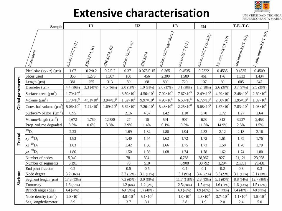
Extensive characterisationSample U4 T.E.-T.GU1 U2 U3

Inst

rum

ent

mic

ro-X

CT

(v1

)

SB

FS

EM

_R

1

SB

FS

EM

_R

2

mic

ro-X

CT

(v2

)

SB

FS

EM

mic

ro-X

CT

(sy

nch

rot.

)

mic

ro-X

CT

(v2

)

mic

ro-X

CT

(v2

-40

X)

1st

mic

ro-X

CT

(v

2)

2nd

mic

ro-X

CT

(v

2)

2_i

mp

mic

ro-X

CT

(v2

)

Glo

ba

l p

ara

mete

rs

Pixel size (xy / z) (µm) 1.07 0.2/0.2 0.2/0.2 0.371 0.075/0.15 0.365 0.4535 0.2322 0.4535 0.4535 0.4509

Slices used 356 1,273 1,567 160 456 2,300 1,589 461 176 1,333 1,434

Length (µm) 381 255 313 59 68 839 720 107 80 605 647

Diameter (µm) 4.4 (39%) 3.3 (45%) 4.5 (56%) 2.0 (18%) 1.0 (31%) 2.6 (37%) 3.1 (38%) 1.2 (28%) 2.6 (38%) 3.7 (37%) 2.5 (25%)

Surface area (µm2) 1.70×10

63.50×10

34.56×10

37.02×10

57.67×10

52.49×10

54.29×10

42.48×10

62.60×10

6

Volume (µm3) 1.78×10

64.51×10

53.94×10

61.62×10

39.97×10

24.96×10

56.53×10

56.72×10

42.50×10

41.95×10

61.59×10

6

Conv. hull volume (µm3) 5.06×10

77.41×10

71.09×10

85.62×10

47.26×10

45.48×10

82.25×10

85.68×10

51.67×10

57.83×10

71.03×10

8

Surface/Volume (µm-1

) 0.95 2.16 4.57 1.42 1.18 3.70 1.72 1.27 1.64

Volume/length (µm2) 4,672 1,769 12,588 27 15 591 907 628 313 3,227 2,453

Prop. volume degraded 3.5% 0.6% 3.6% 2.9% 1.4% 0.1% 0.3% 11.8% 14.9% 2.5% 1.5%

3DDf 2.23 1.69 1.84 1.80 1.94 2.33 2.12 2.18 2.16

xy 2D

Df 1.83 1.40 1.54 1.62 1.72 1.72 1.61 1.75 1.76

xz 2D

Df 1.83 1.42 1.58 1.66 1.75 1.73 1.58 1.76 1.79

yz 2D

Df 1.86 1.50 1.56 1.68 1.74 1.78 1.62 1.74 1.80

Number of nodes 5,040 78 504 6,768 28,967 927 21,121 23,028

Number of segments 6,191 78 510 6,908 38,792 1,294 21,051 29,431

End point fraction 0.2 0.5 0.5 0.4 0.1 0.2 0.3 0.3

Node degree 3.2 (16%) 3.2 (12%) 3.1 (11%) 3.1 (9%) 3.4 (22%) 3.3 (20%) 3.1 (11%) 3.1 (10%)

Segment length (µm) 17.3 (93%) 7.3 (60%) 3.0 (63%) 11.7 (118%) 2.3 (63%) 5.1 (60%) 8.8 (94%) 12.7 (86%)

Tortuosity 1.6 (37%) 1.2 (6%) 1.2 (7%) 2.5 (38%) 1.5 (6%) 1.6 (11%) 1.6 (13%) 1.5 (12%)

Branch angle (deg) 64 (47%) 69 (39%) 57 (48%) 63 (49%) 69 (46%) 67 (43%) 64 (47%) 60 (45%)

Node density (µm-3

) 2.8×10-3

4.8×10-2

5.1×10-1

1.0×10-2

4.3×10-1

3.7×10-2

1.1×10-2

1.5×10-2

Seg. length/diameter 3.9 3.7 3.1 3.8 1.9 2.0 2.4 5.0

Glo

ba

l p

ara

mete

rs

Fra

cta

lS

kele

ton

TEMA 2

La dinámica de las descargas parciales

36

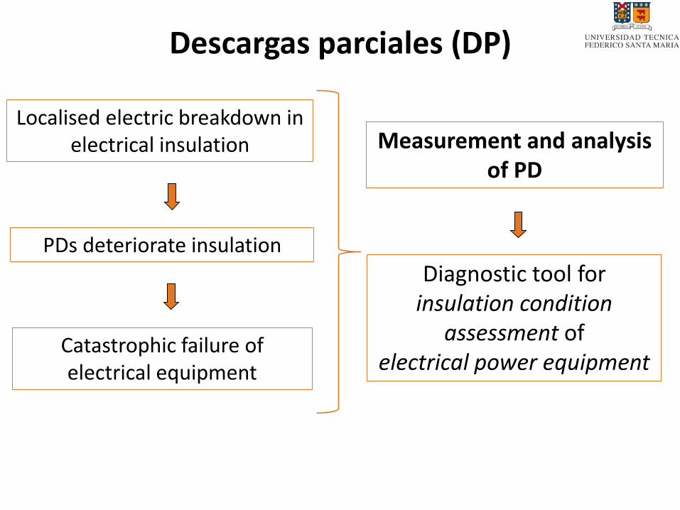
Descargas parciales (DP)

Localised electric breakdown in electrical insulation

PDs deteriorate insulation

Catastrophic failure of electrical equipment

Measurement and analysis of PD

Diagnostic tool forinsulation condition

assessment ofelectrical power equipment

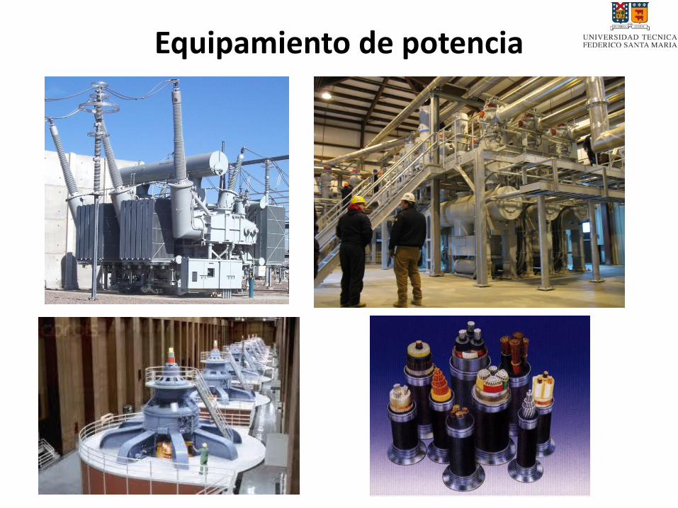
Equipamiento de potencia

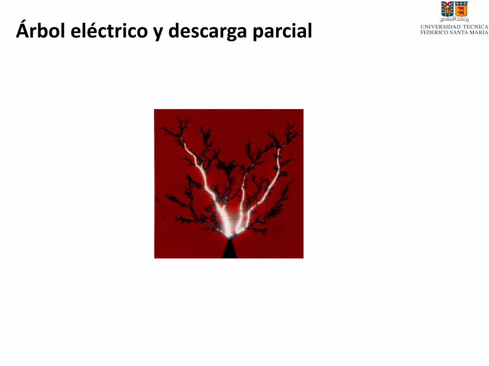
Árbol eléctrico y descarga parcial

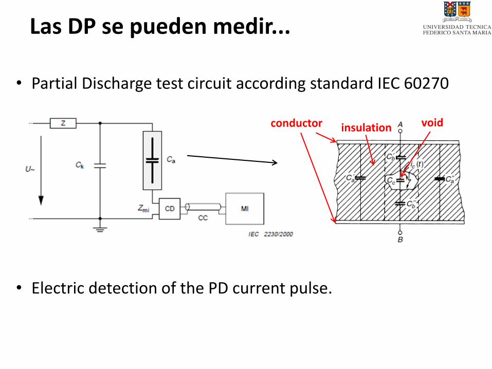
Las DP se pueden medir...

• Partial Discharge test circuit according standard IEC 60270

• Electric detection of the PD current pulse.

voidinsulationconductor

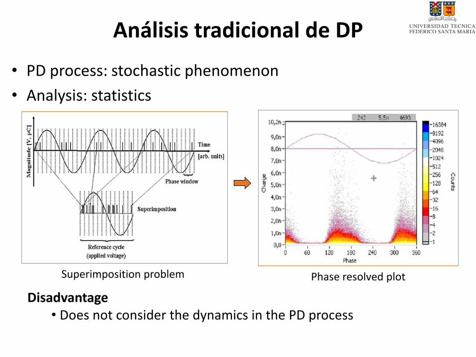
Análisis tradicional de DP

Phase resolved plot

Disadvantage• Does not consider the dynamics in the PD process

• PD process: stochastic phenomenon

• Analysis: statistics

Superimposition problem

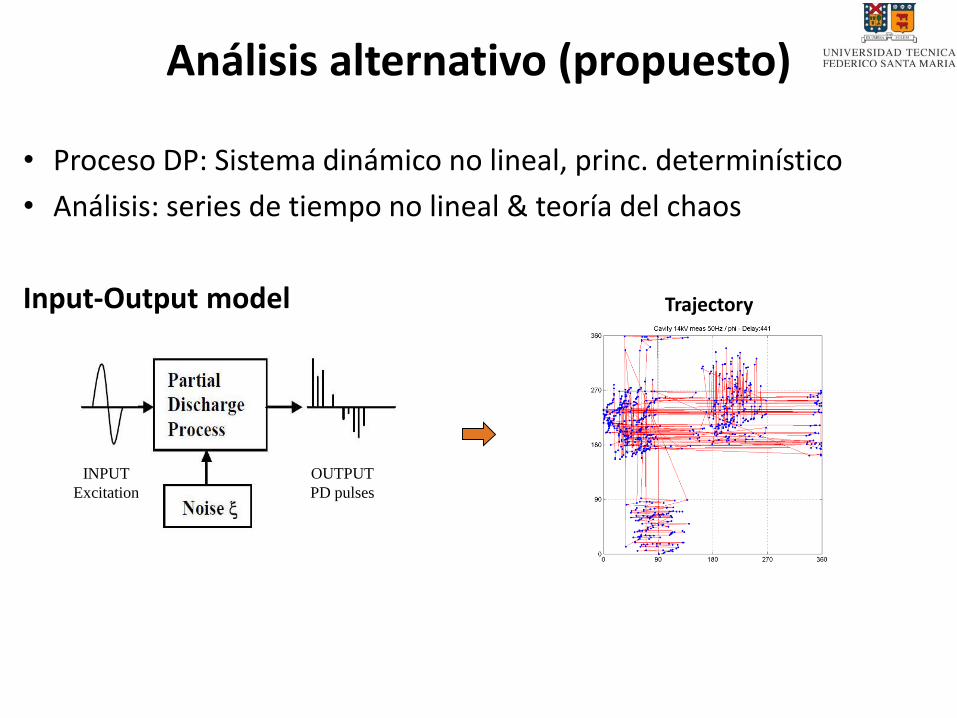
Análisis alternativo (propuesto)

INPUT

Excitation

OUTPUT

PD pulses

Trajectory

• Proceso DP: Sistema dinámico no lineal, princ. determinístico

• Análisis: series de tiempo no lineal & teoría del chaos

Input-Output model

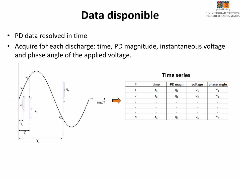
Data disponible

• PD data resolved in time

• Acquire for each discharge: time, PD magnitude, instantaneous voltage and phase angle of the applied voltage.

Time series

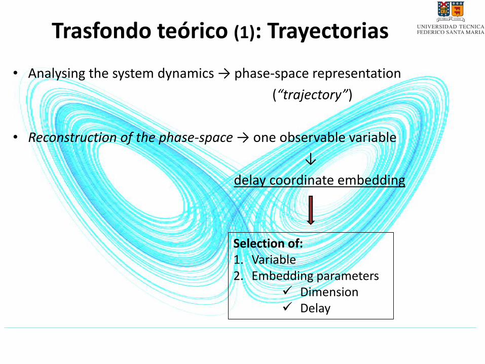
Trasfondo teórico (1): Trayectorias

• Analysing the system dynamics → phase-space representation

(“trajectory”)

• Reconstruction of the phase-space → one observable variable

↓

delay coordinate embedding

Selection of:1. Variable2. Embedding parameters

Dimension Delay

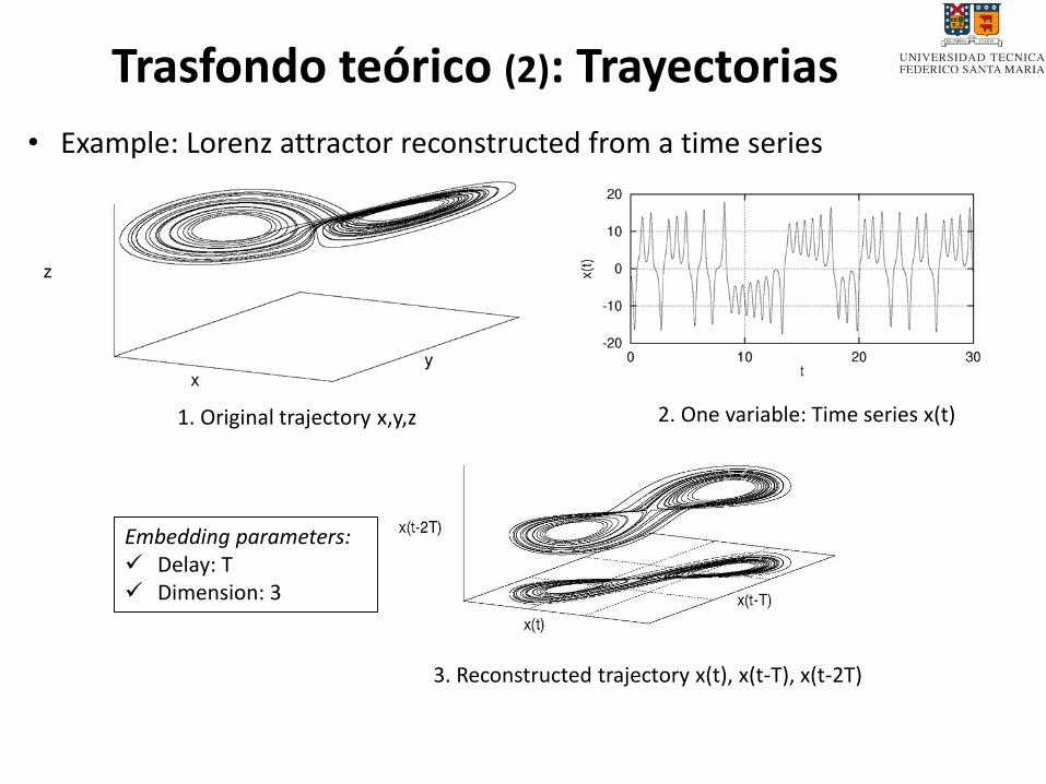
• Example: Lorenz attractor reconstructed from a time series

1. Original trajectory x,y,z 2. One variable: Time series x(t)

3. Reconstructed trajectory x(t), x(t-T), x(t-2T)

Embedding parameters: Delay: T Dimension: 3

Trasfondo teórico (2): Trayectorias

Objetivos del estudio

GRAL: Estudiar el comportamiento dinámico de las DP

• Relacionar defectos de DP con patrones de DP

• Evaluar la potencialidad del método propuesto

• Evaluar la capacidad del método para:

Identificar fuentes de DP simultáneas

usarlo para el diagnóstico del envejecimiento del aislamiento eléctrico

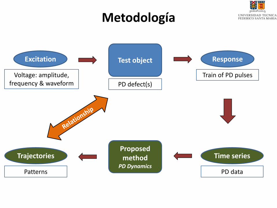
Metodología

Excitation Test object

Voltage: amplitude, frequency & waveform

Response

PD defect(s)

Train of PD pulses

TrajectoriesProposed method

PD DynamicsPatterns

Time series

PD data

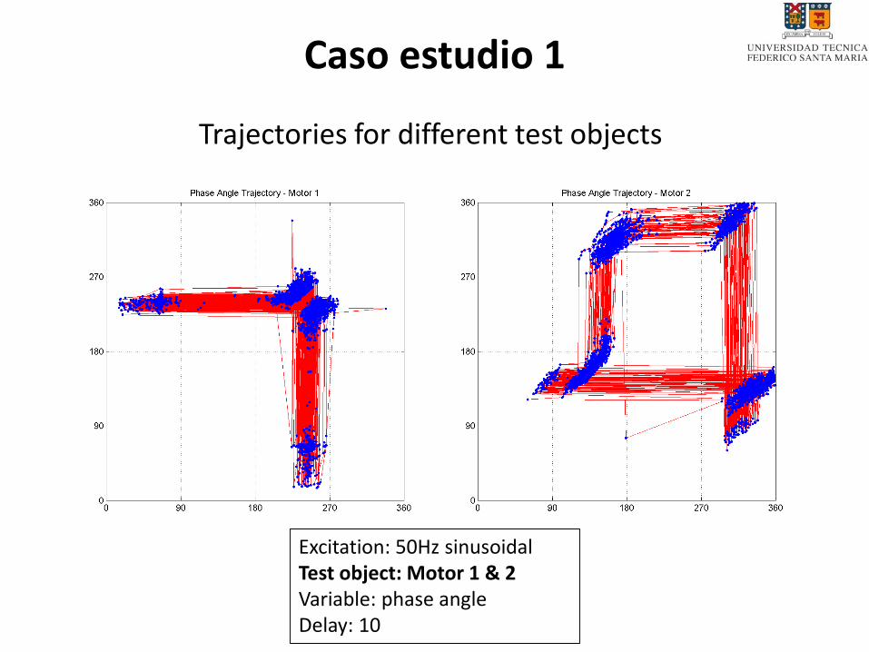
Caso estudio 1

Trajectories for different test objects

Excitation: 50Hz sinusoidalTest object: Motor 1 & 2Variable: phase angleDelay: 10

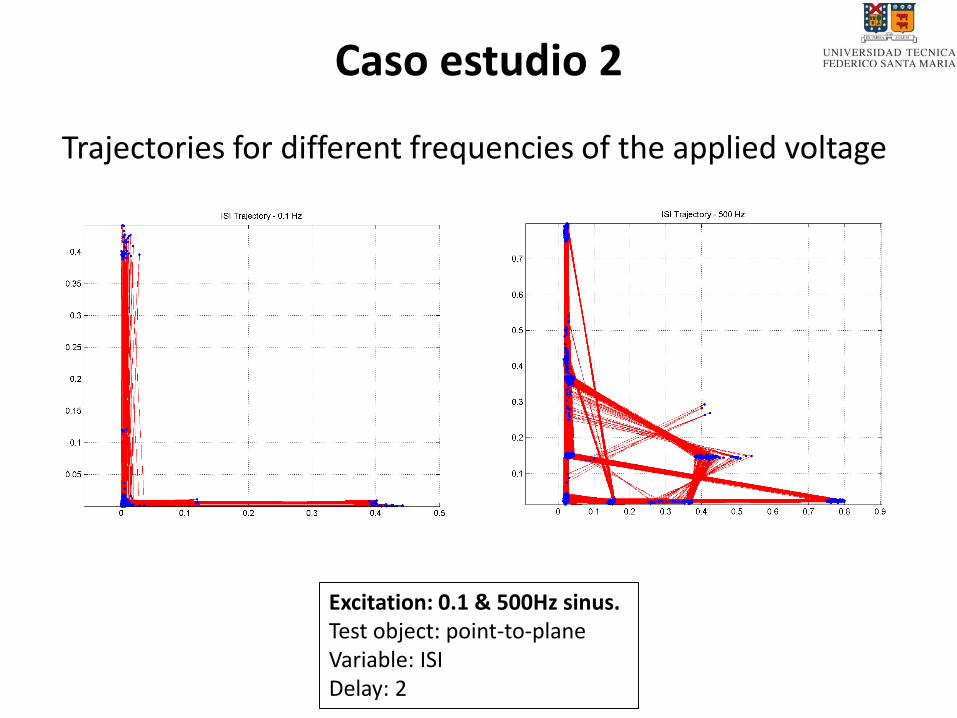
Caso estudio 2

Trajectories for different frequencies of the applied voltage

Excitation: 0.1 & 500Hz sinus.Test object: point-to-planeVariable: ISIDelay: 2

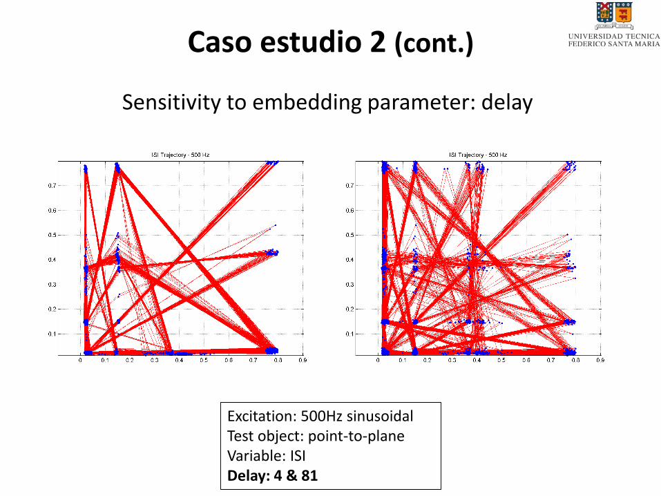
Caso estudio 2 (cont.)

Sensitivity to embedding parameter: delay

Excitation: 500Hz sinusoidalTest object: point-to-planeVariable: ISIDelay: 4 & 81

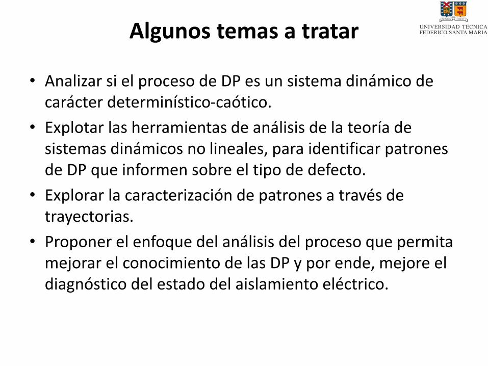
Algunos temas a tratar

• Analizar si el proceso de DP es un sistema dinámico de carácter determinístico-caótico.

• Explotar las herramientas de análisis de la teoría de sistemas dinámicos no lineales, para identificar patrones de DP que informen sobre el tipo de defecto.

• Explorar la caracterización de patrones a través de trayectorias.

• Proponer el enfoque del análisis del proceso que permita mejorar el conocimiento de las DP y por ende, mejore el diagnóstico del estado del aislamiento eléctrico.

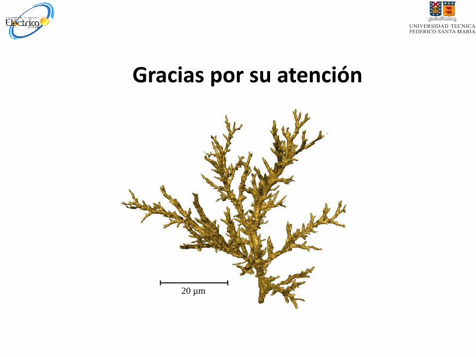
Gracias por su atención

20 µm

Extra slides

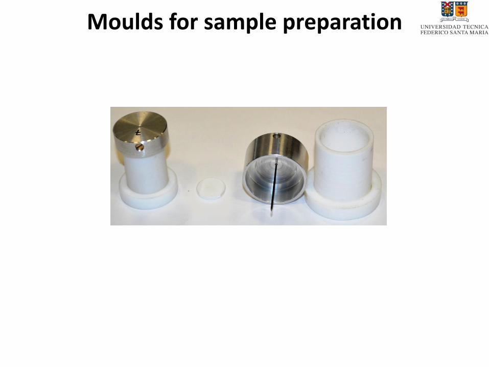
Moulds for sample preparation

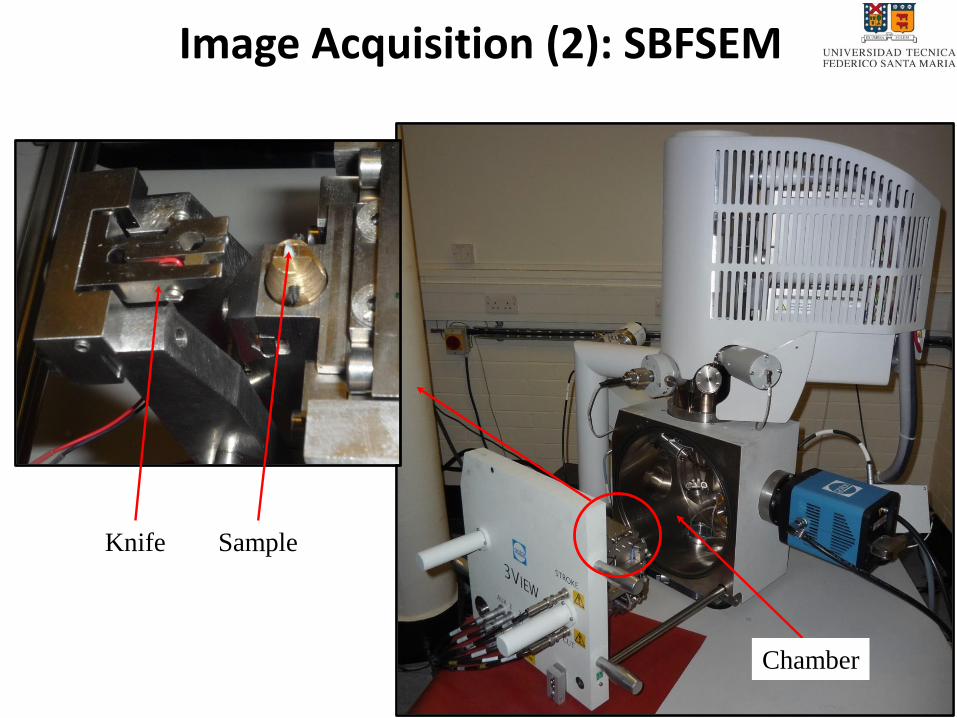
Image Acquisition (2): SBFSEM

SampleKnife

Chamber

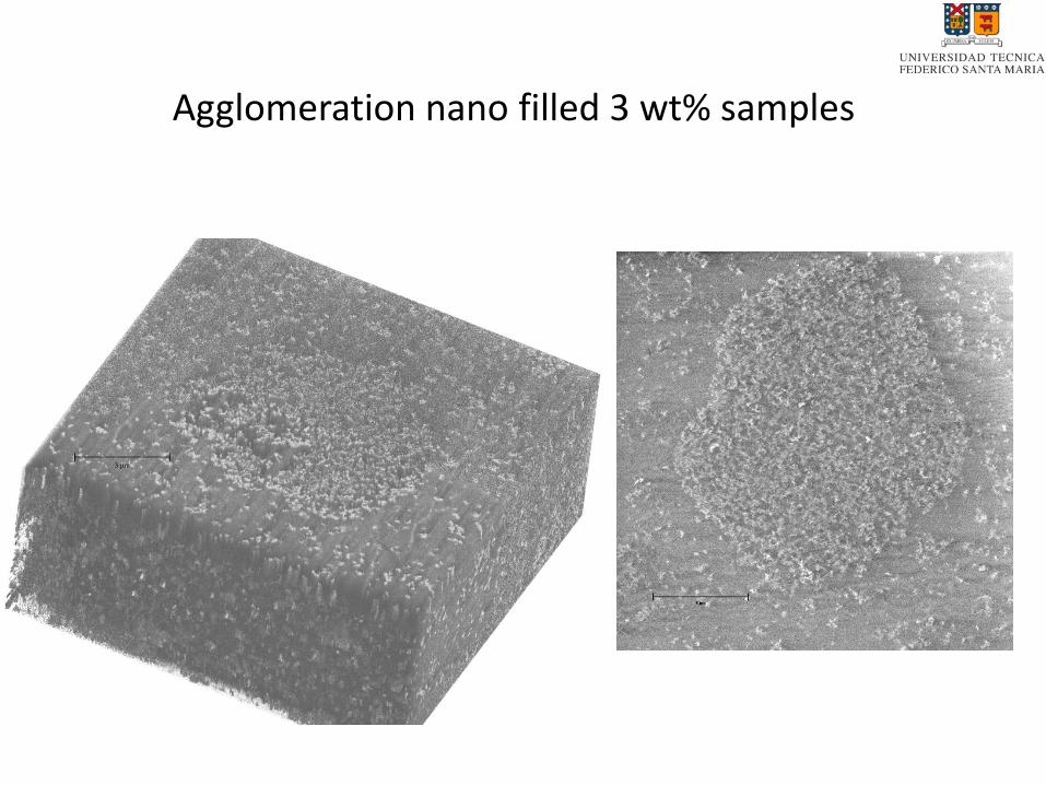
Agglomeration nano filled 3 wt% samples

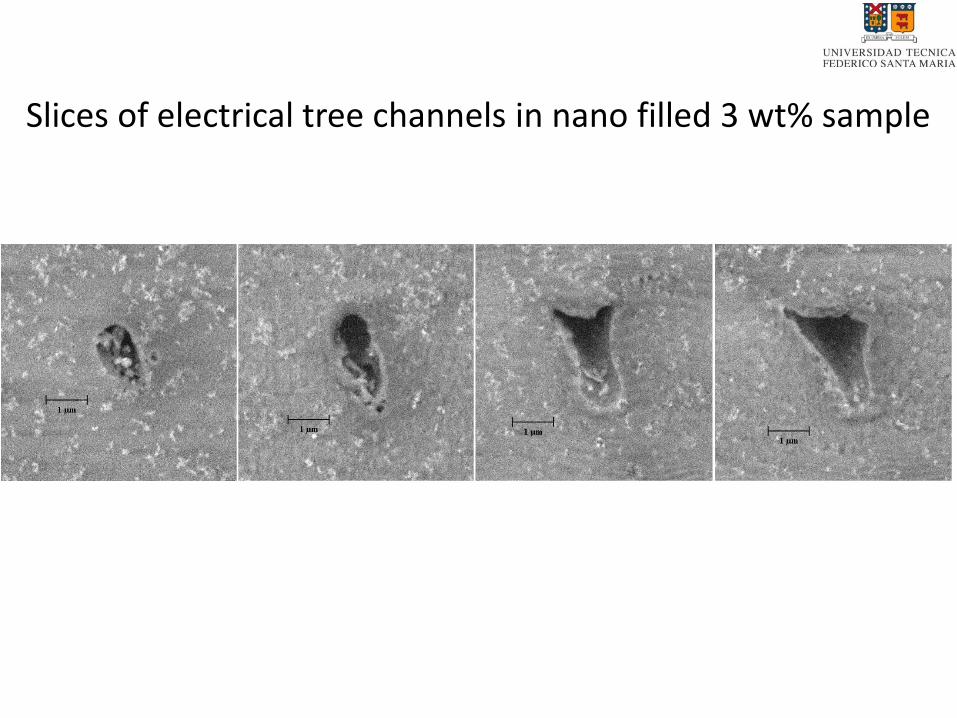
Slices of electrical tree channels in nano filled 3 wt% sample

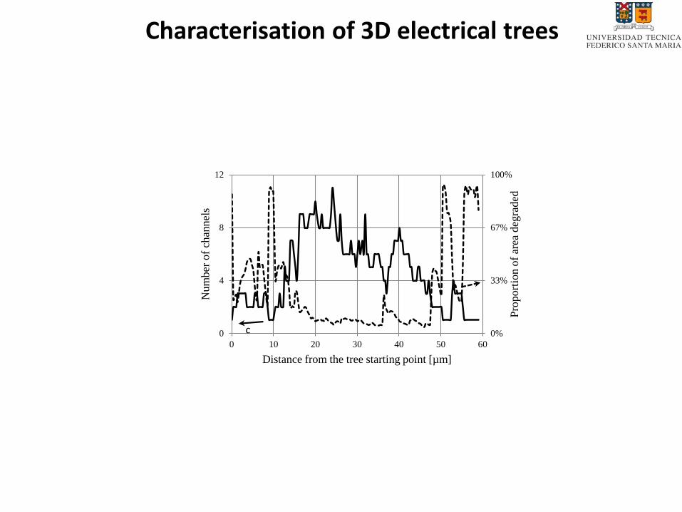
Characterisation of 3D electrical trees

0%

33%

67%

100%

0

4

8

12

0 10 20 30 40 50 60

Pro

port

ion o

f ar

ea d

egra

ded

Num

ber

of

chan

nel

s

Distance from the tree starting point [µm]

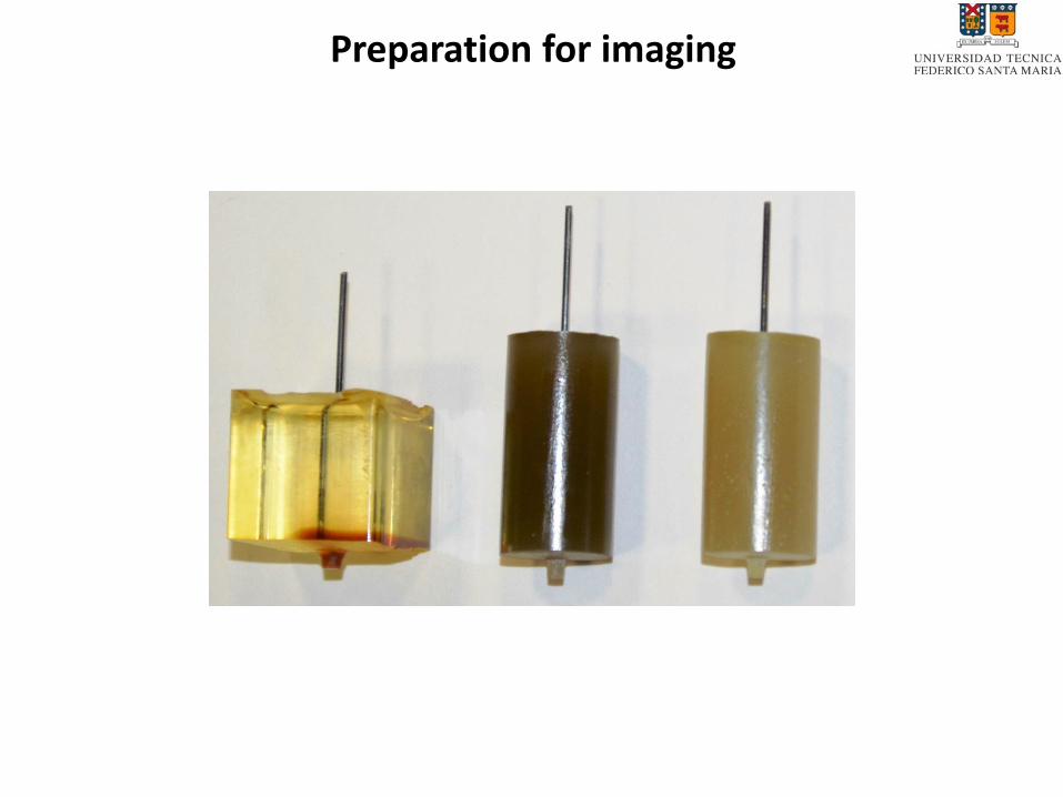
Preparation for imaging

End