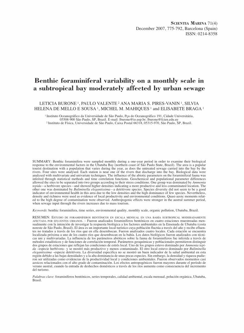
Estudio de foraminífiros bentónicos en escala mensual en una bahía subtropical moderadamente afectada por efluentes urbanos

SCIENTIA MARINA 71(4)December 2007, 775-792, Barcelona (Spain)

ISSN: 0214-8358

Benthic foraminiferal variability on a monthly scale ina subtropical bay moderately affected by urban sewage

LETICIA BURONE 1, PAULO VALENTE 2 ANA MARIA S. PIRES-VANIN 1, SILVIAHELENA DE MELLO E SOUSA 1, MICHEL M. MAHIQUES 1 and ELISABETE BRAGA 1

1 Instituto Oceanográfico da Universidade de São Paulo, Pça do Oceanográfico 191, Cidade Universitária, 05508-900 São Paulo, SP, Brazil. E-mail: [email protected]; [email protected]

2 Instituto de Física, Universidade de São Paulo, Caixa Postal 66318, 05315-970, São Paulo, SP, Brazil.

SUMMARY: Benthic foraminifera were sampled monthly during a one-year period in order to examine their biologicalresponse to the environmental factors in the Ubatuba Bay (northern coast of São Paulo State, Brazil). The area is a populartourist destination with a population that varies during the year, as does the untreated sewage carried into the bay by therivers. Four sites were analysed. Each station is near one of the rivers that discharge into the bay. Biological data wereanalysed with multivariate and univariate techniques. The influence of the abiotic parameters on the foraminiferal fauna wasinferred through statistical methods and time correlation functions. Geochemical and populational parameter differencesallowed the sites to be separated into two groups according to their stress conditions. One group was dominated by Ammoniatepida—a herbivore species—and showed higher densities indicating a more productive and less contaminated location. Theother one was dominated by Buliminella elegantissima—a detritivore species. Species diversity did not seem to be a goodindicator of environmental health in this area due to the low densities and the high dominance of few species. Nevertheless,density and richness were used as evidence of local productivity and environmental conditions. Quasi-azoic moments relat-ed to the high degree of contamination were observed. Anthropogenic effects were stronger in the austral summer period,when sewage input through the rivers increases due to mass tourism.

Keywords: benthic foraminifera, time series, environmental quality, monthly scale, organic pollution, Ubatuba, Brazil.

RESUMEN: ESTUDIO DE FORAMINÍFEROS BENTÓNICOS EN ESCALA MENSUAL EN UNA BAHÍA SUBTROPICAL MODERADAMENTEAFECTADA POR EFLUENTES URBANOS. – Fueron analizados foraminíferos bentónicos en cuatro estaciones muestreadas men-sualmente con la intención de investigar la respuesta biológica a los factores ambientales en la Ensenada de Ubatuba (costanoreste de São Paulo, Brasil). El área es un importante local turístico cuya población fluctúa a través del año y recibe efluen-tes no tratados a través de los ríos que en ella desembocan. Fueron analizados cuatro locales. Cada estación se encuentralocalizada próxima a uno de los cuatro ríos que desembocan en la bahía. Los datos biológicos fueron analizados con técni-cas uni y multivariadas. La influencia de los parámetros abióticos sobre la fauna de foraminíferos fue inferida a través demétodos estadísticos y de funciones de correlación temporal. Parámetros geoquímicas y poblacionales permitieron distinguirdos grupos de estaciones que reflejan las condiciones de estrés local. Uno de los grupos estuvo dominado por Ammonia tepi-da –especie herbívora– y se mostró más productivo y menos contaminado. El otro local estuvo dominado por Buliminellaelegantissima –especie detritívora. La diversidad especifica no se mostró un buen indicador de la salud ambiental en estaregión debido a las bajas densidades y a la alta dominancia de unas pocas especies. Sin embargo, la densidad y riqueza pudie-ron ser utilizadas como evidencias de la productividad local y condiciones ambientales. Fueron observados momentos casiazoicos relacionados con el alto grado de contaminación. Los efectos antropogénicos fueron mayores durante el período deverano austral, cuando la entrada de deshechos domésticos a través de los ríos aumenta como consecuencia del incrementodel turismo.

Palabras clave: foraminíferos bentónicos, series temporales, calidad ambiental, escala mensual, polución orgánica, Ubatuba,Brasil.

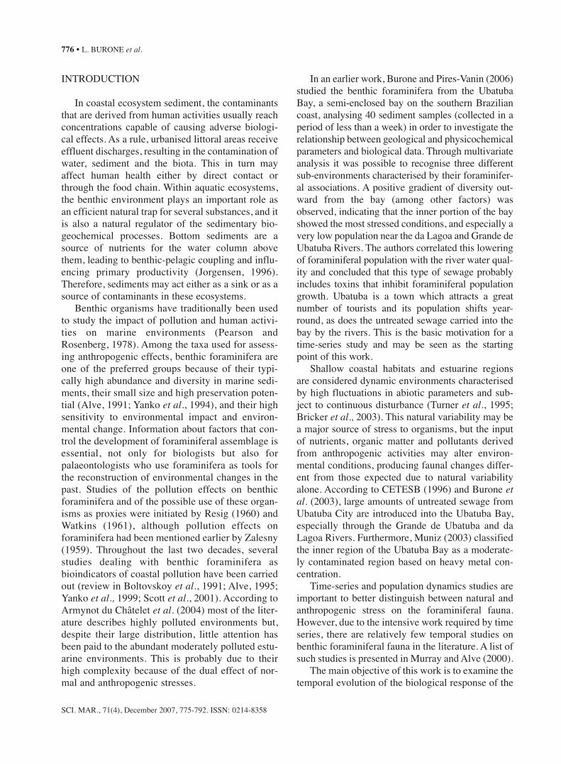
INTRODUCTION

In coastal ecosystem sediment, the contaminantsthat are derived from human activities usually reachconcentrations capable of causing adverse biologi-cal effects. As a rule, urbanised littoral areas receiveeffluent discharges, resulting in the contamination ofwater, sediment and the biota. This in turn mayaffect human health either by direct contact orthrough the food chain. Within aquatic ecosystems,the benthic environment plays an important role asan efficient natural trap for several substances, and itis also a natural regulator of the sedimentary bio-geochemical processes. Bottom sediments are asource of nutrients for the water column abovethem, leading to benthic-pelagic coupling and influ-encing primary productivity (Jorgensen, 1996).Therefore, sediments may act either as a sink or as asource of contaminants in these ecosystems.

Benthic organisms have traditionally been usedto study the impact of pollution and human activi-ties on marine environments (Pearson andRosenberg, 1978). Among the taxa used for assess-ing anthropogenic effects, benthic foraminifera areone of the preferred groups because of their typi-cally high abundance and diversity in marine sedi-ments, their small size and high preservation poten-tial (Alve, 1991; Yanko et al., 1994), and their highsensitivity to environmental impact and environ-mental change. Information about factors that con-trol the development of foraminiferal assemblage isessential, not only for biologists but also forpalaeontologists who use foraminifera as tools forthe reconstruction of environmental changes in thepast. Studies of the pollution effects on benthicforaminifera and of the possible use of these organ-isms as proxies were initiated by Resig (1960) andWatkins (1961), although pollution effects onforaminifera had been mentioned earlier by Zalesny(1959). Throughout the last two decades, severalstudies dealing with benthic foraminifera asbioindicators of coastal pollution have been carriedout (review in Boltovskoy et al., 1991; Alve, 1995;Yanko et al., 1999; Scott et al., 2001). According toArmynot du Châtelet et al. (2004) most of the liter-ature describes highly polluted environments but,despite their large distribution, little attention hasbeen paid to the abundant moderately polluted estu-arine environments. This is probably due to theirhigh complexity because of the dual effect of nor-mal and anthropogenic stresses.

In an earlier work, Burone and Pires-Vanin (2006)studied the benthic foraminifera from the UbatubaBay, a semi-enclosed bay on the southern Braziliancoast, analysing 40 sediment samples (collected in aperiod of less than a week) in order to investigate therelationship between geological and physicochemicalparameters and biological data. Through multivariateanalysis it was possible to recognise three differentsub-environments characterised by their foraminifer-al associations. A positive gradient of diversity out-ward from the bay (among other factors) wasobserved, indicating that the inner portion of the bayshowed the most stressed conditions, and especially avery low population near the da Lagoa and Grande deUbatuba Rivers. The authors correlated this loweringof foraminiferal population with the river water qual-ity and concluded that this type of sewage probablyincludes toxins that inhibit foraminiferal populationgrowth. Ubatuba is a town which attracts a greatnumber of tourists and its population shifts year-round, as does the untreated sewage carried into thebay by the rivers. This is the basic motivation for atime-series study and may be seen as the startingpoint of this work.

Shallow coastal habitats and estuarine regionsare considered dynamic environments characterisedby high fluctuations in abiotic parameters and sub-ject to continuous disturbance (Turner et al., 1995;Bricker et al., 2003). This natural variability may bea major source of stress to organisms, but the inputof nutrients, organic matter and pollutants derivedfrom anthropogenic activities may alter environ-mental conditions, producing faunal changes differ-ent from those expected due to natural variabilityalone. According to CETESB (1996) and Burone etal. (2003), large amounts of untreated sewage fromUbatuba City are introduced into the Ubatuba Bay,especially through the Grande de Ubatuba and daLagoa Rivers. Furthermore, Muniz (2003) classifiedthe inner region of the Ubatuba Bay as a moderate-ly contaminated region based on heavy metal con-centration.

Time-series and population dynamics studies areimportant to better distinguish between natural andanthropogenic stress on the foraminiferal fauna.However, due to the intensive work required by timeseries, there are relatively few temporal studies onbenthic foraminiferal fauna in the literature. A list ofsuch studies is presented in Murray and Alve (2000).

The main objective of this work is to examine thetemporal evolution of the biological response of the

SCI. MAR., 71(4), December 2007, 775-792. ISSN: 0214-8358

776 • L. BURONE et al.

benthic foraminifera to the environmental parameterchanges. Emphasis is given to a comparison of theexamined sites.

MATERIALS AND METHODS

Study Area

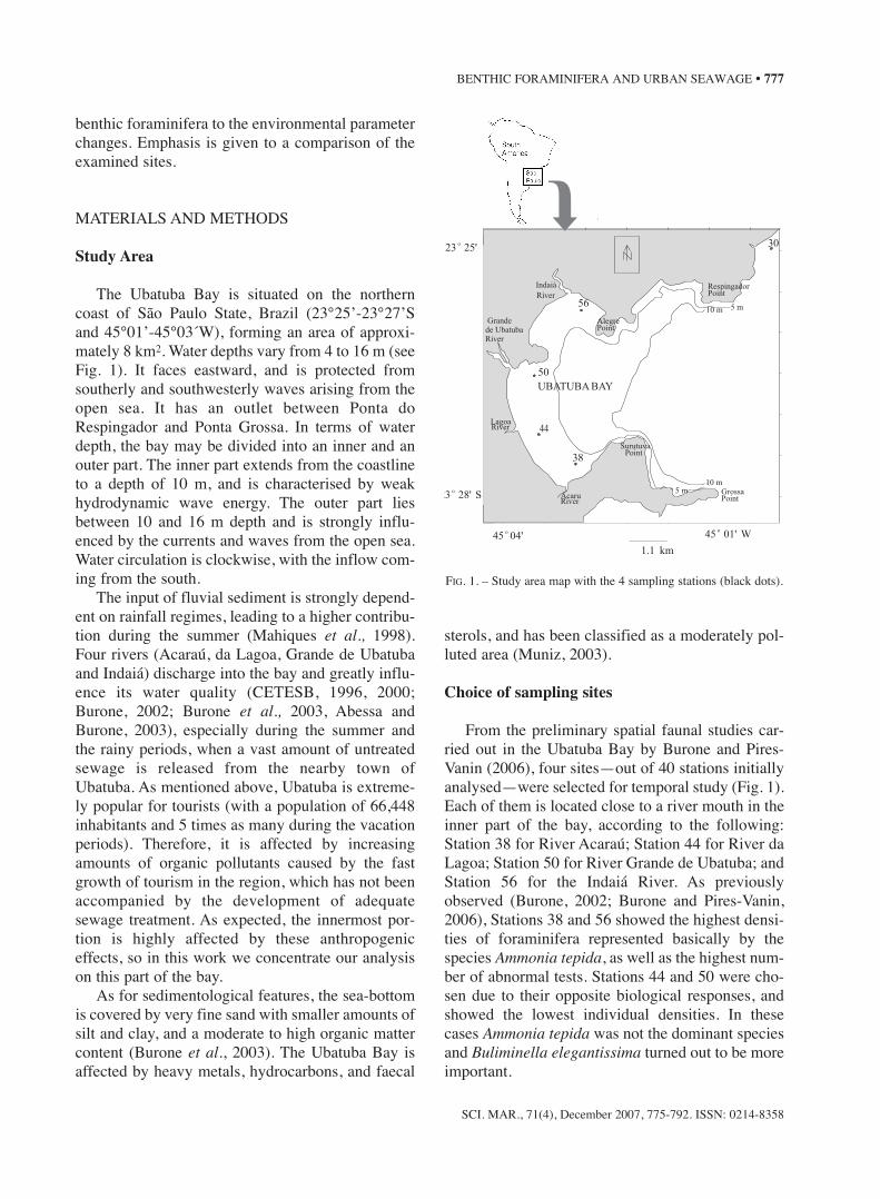
The Ubatuba Bay is situated on the northerncoast of São Paulo State, Brazil (23°25’-23°27’Sand 45°01’-45°03´W), forming an area of approxi-mately 8 km2. Water depths vary from 4 to 16 m (seeFig. 1). It faces eastward, and is protected fromsoutherly and southwesterly waves arising from theopen sea. It has an outlet between Ponta doRespingador and Ponta Grossa. In terms of waterdepth, the bay may be divided into an inner and anouter part. The inner part extends from the coastlineto a depth of 10 m, and is characterised by weakhydrodynamic wave energy. The outer part liesbetween 10 and 16 m depth and is strongly influ-enced by the currents and waves from the open sea.Water circulation is clockwise, with the inflow com-ing from the south.

The input of fluvial sediment is strongly depend-ent on rainfall regimes, leading to a higher contribu-tion during the summer (Mahiques et al., 1998).Four rivers (Acaraú, da Lagoa, Grande de Ubatubaand Indaiá) discharge into the bay and greatly influ-ence its water quality (CETESB, 1996, 2000;Burone, 2002; Burone et al., 2003, Abessa andBurone, 2003), especially during the summer andthe rainy periods, when a vast amount of untreatedsewage is released from the nearby town ofUbatuba. As mentioned above, Ubatuba is extreme-ly popular for tourists (with a population of 66,448inhabitants and 5 times as many during the vacationperiods). Therefore, it is affected by increasingamounts of organic pollutants caused by the fastgrowth of tourism in the region, which has not beenaccompanied by the development of adequatesewage treatment. As expected, the innermost por-tion is highly affected by these anthropogeniceffects, so in this work we concentrate our analysison this part of the bay.

As for sedimentological features, the sea-bottomis covered by very fine sand with smaller amounts ofsilt and clay, and a moderate to high organic mattercontent (Burone et al., 2003). The Ubatuba Bay isaffected by heavy metals, hydrocarbons, and faecal

sterols, and has been classified as a moderately pol-luted area (Muniz, 2003).

Choice of sampling sites

From the preliminary spatial faunal studies car-ried out in the Ubatuba Bay by Burone and Pires-Vanin (2006), four sites—out of 40 stations initiallyanalysed—were selected for temporal study (Fig. 1).Each of them is located close to a river mouth in theinner part of the bay, according to the following:Station 38 for River Acaraú; Station 44 for River daLagoa; Station 50 for River Grande de Ubatuba; andStation 56 for the Indaiá River. As previouslyobserved (Burone, 2002; Burone and Pires-Vanin,2006), Stations 38 and 56 showed the highest densi-ties of foraminifera represented basically by thespecies Ammonia tepida, as well as the highest num-ber of abnormal tests. Stations 44 and 50 were cho-sen due to their opposite biological responses, andshowed the lowest individual densities. In thesecases Ammonia tepida was not the dominant speciesand Buliminella elegantissima turned out to be moreimportant.


BENTHIC FORAMINIFERA AND URBAN SEAWAGE • 777

-45.07 -45.06 -45.05 -45.04 -45.03 -45.02 -45.01

-23.46

-23.45

-23.44

-23.43

-23.42

-23.41

-23.4030

38

50

56

UBATUBABAY

Indaiá

River

Grandede UbatubaRiver

LagoaRiver

AcaruRiver

GrossaPoint

RespingadorPoint

5 m10 m

5 m10 m

AlegrePoint

SurutuvaPoint

1.1 km

45 01' Wo

45 04'o

23 25'o

23 28' So

44

FIG. 1. – Study area map with the 4 sampling stations (black dots).

Sampling procedure

Sampling was performed monthly at Stations 38,44, 50 and 56 from October 1998 to October 1999.Sediment samples were taken with a Kajak-Brinkurst corer sampler (10 cm internal diameter,penetrating the sediment by gravity) on board theresearch vessel Veliger II.

To study the living benthic foraminiferal fauna,the uppermost 3 cm of the core was removed, form-ing a volume of about 230 cm3 per sample. All of thesamples had the same volume and all living individ-uals were sorted out. In order to differentiatebetween living and dead foraminifera the materialwas stained with buffered Bengal Rose dye (1 g ofBengal Rose in 1000 ml of distilled water) for 48hours (Walton, 1952). The wet samples were thencarefully washed in the laboratory through 0.500,0.250 and 0.062 mm sieves to segregate the sizefractions. After drying at 60°C, the remaining por-tion in the smaller sieve was submitted to flotationwith carbon trichloroethylene. The floated materialwas transferred to filter paper and air-dried. All theliving specimens in each sample were picked andidentified following the generic classification ofLoeblich and Tappan (1988). Species were classifiedby their feeding strategy according to Murray(1991).

Separate samples were taken for organic carbon,nitrogen and grain size analysis. Organic carbon andnitrogen were determined using 500 mg of freeze-dried and weighted sediment. The samples weredecarbonated with a 1 M solution of hydrochloricacid, washed 3 times with deionised water, freeze-dried and then analysed in a LECO CNS 2000.Granulometric composition was analysed using aMalvern 2000 low-angle laser light scattering(LALLS) instrument, and the size intervals wereclassified using the Wenthworth scale (Wentworth1922 in Suguio, 1973).

To study pore water ammonium (NH4+pw) and

phosphate (PO43- pw) ion concentrations, the sedi-

ment was placed inside a glove box installed onboard, filled with inert gas (N2) and completelysealed immediately after sampling. Then, the sedi-ment was stored in plastic bottles and kept at a tem-perature of –20°C until the pore water was extractedin the laboratory. The extraction was performed bysediment centrifugation and all of the analyses weremade in oxygen-free atmospheres as described byBurone et al. (2005). The ammonium analysis fol-

lowed the traditional colorimetric method describedin Tréguer and Le Corre (1975) and phosphate wasdetermined colorimetrically as presented inGrasshoff et al. (1983).

The chlorophyll a (Chl a) content of surface sed-iments was determined according to Lorenzen(1967) and Strickland and Parson (1968).Nevertheless, its composition is basically constantover the year, so it was disregarded in the temporalanalysis.

In addition to the sediment sampling, bottomwater samples were taken by means of Nansen bot-tles to study the following variables: temperature(T), dissolved oxygen content (O2), salinity (Sal),pH, and ammonium (NH4

+bw) and phosphate (PO43-

bw) concentrations. The temperature of the bottomwater was measured by means of reversing ther-mometers. Salinity was determined in the laboratoryby a salinometer using a PSU scale; pH was meas-ured on board using a Digimed model DM-2 pH-meter. Dissolved oxygen content was measured bythe Winkler titration method (Grasshoff et al.,1983). To determine the nutrients in the bottomwater, the samples were frozen to be analysed in thelaboratory. The phosphate concentration was deter-mined using a Technicon Auto-Analyzer II accord-ing to the recommendations described by Grasshoffet al. (1983), and the ammonium concentration wasdetermined following the method described byTréguer and Le Corre (1975).

Data analysis

In the laboratory all the living foraminiferal indi-viduals were counted. The data were analysed usingunivariate and multivariate methods. Diversity (H’)was calculated on a natural logarithmic basis (ln x)by the Shannon-Wiener index (Shannon and Weaver1963); the evenness (J’) was calculated according toPielou (1975); and species richness (S) was deter-mined as the total number of species.

A principal component analysis (PCA) was car-ried out for the ordination of sample locations forthe abiotic factors. A first matrix (previously nor-malised and centred) was constructed using the totalof variables measured. However, in order to avoidredundancy and perform a more realistic ordination,the variables with a low percentage of contributionwere eliminated. Therefore, a second matrix wasobtained using a total of 12 variables: total organiccarbon (C), fine sand (FS), very fine sand (VFS),



silt, Salinity, O2, pH, chlorophyll a (Chl a), ammo-nium dissolved in the water column (NH4

+bw),phosphate dissolved in the water column (PO4

3-bw),ammonium dissolved in the pore water (NH4

+pw)and phosphate dissolved in the pore water (PO4

3-pw).As a first approximation for the analysis of the

relation between the biotic and abiotic variables, aPearson correlation analysis was performed consid-ering p <0.05 as the significant level.

In order to analyse the temporal response of theforaminiferal community, we applied several statis-tical tools. At first we calculated the autocorrelationcoefficient for each station, defined by

, (1)

where yi is the data in the time i, y– is the mean value(averaged through the year), yi+τ is the data in thetime i+τ and τ is a lag time. We calculated the R(τ)coefficient for each data set (biotic and abioticparameters) and each station. Equation 1 wasreferred to as a Time Series Analysis (Wilson andDawe, 2006) and proved to be a useful tool for evi-dencing periodic behaviours in foraminiferal com-munities. The time profile of the R(τ) functionreveals the periodicity of the corresponding data set,if such periodicity exists. Similarly, we also calcu-lated the cross-correlation function for some chosenpairs of variables, defined by

, (2)

where y and z are two different variables. Because τis always a positive lag time, we chose y with careas an independent parameter (usually an abiotic one)and z as the dependent one. Thus, Ryz(τ) may give anestimate of the response time for the variable z as aresult of the action of y. For τ = 0, Ryz(τ = 0) corre-sponds to a usual linear correlation.

The possible seasonal environment effect and itsbiotic response over time were analysed using a non-metric multi-dimensional ordination (nMDS; Kruskaland Wish, 1978). This nMDS ordinates groups of sta-tions with similar foraminiferal fauna structure and

was performed using the abundance similarity matrix,where the Bray-Curtis similarity index was used (Brayand Curtis, 1957). Four seasonal matrix data wereconstructed, one for each season according to the def-inition: Spring (October, November and December),Summer (January, February and March); Autumn(April, May and June); and Winter (July, August andSeptember). Data were transformed by the square-roottransformation.

Once the temporal data had been obtained wecalculated the annual average values of the popula-tion parameters (H–’, J–’, S– and D–). Since J–’, S– andD– were calculated using simple arithmetic averages,H–’ was obtained with a geometric average, weight-ed by richness (Burone and Pires-Vannin, 2006)

, (3)

where H’ki and Ski are diversity and richness of thestation k at month i, respectively. This annual meangives a good characterisation of each studied site.

To perform uni- and multivariate techniques weused the Multivariate Statistical Package (MVSP)(Kovach, 1999) and the PRIMER package (version5.0, Clarke and Warwick, 2001).

RESULTS

Environmental variables

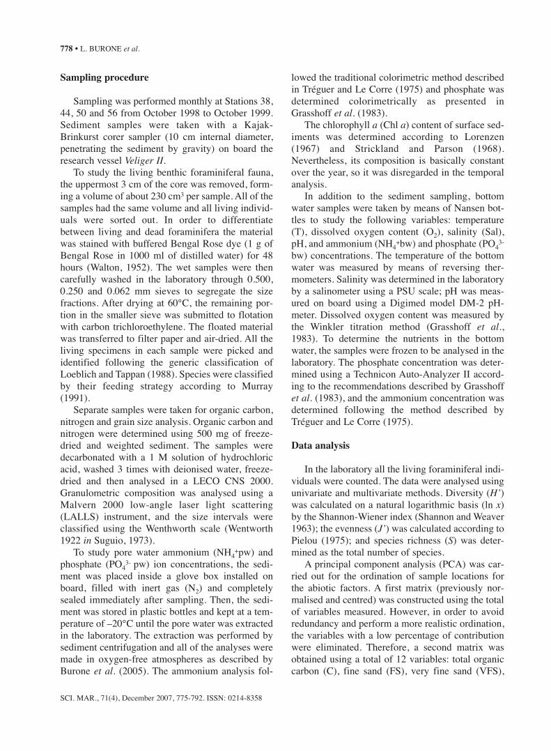
Water temperature (Fig. 2) ranged from 20.3 to30.3°C and showed maximum values in summer andminimum ones in winter, with an expected seasonalpattern. Salinity values ranged between 31.5 and 35.On average, the lowest values were registered atStation 50, as a consequence of the Grande deUbatuba River which, among the four tributary bayrivers, has the highest river discharge. In general, thepH values lay around 8.0, revealing slightly basicwater. Nevertheless, a highly acid condition (pH ≅6.0) was found at Station 50 for November,December and January. This may be related to thelow oxygen concentration registered at this station(3.2 and 3.9 ml/l) and to the maximum carbon con-centration shown below 1.44%.

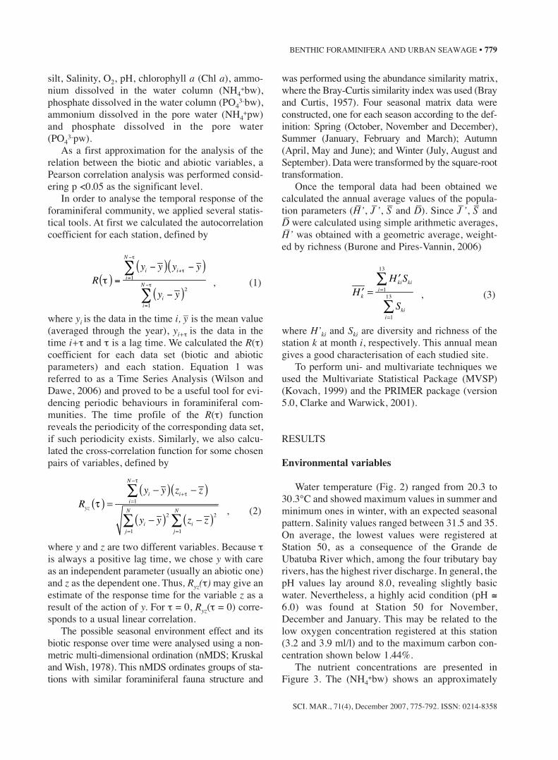
The nutrient concentrations are presented inFigure 3. The (NH4

+bw) shows an approximately

′Hk =′HkiSki

i=1

13

∑

Skii=1

13

∑

Ryz τ( ) =yi − y( ) zi+τ − z( )

i=1

N −τ

∑

yi − y( )2 zi − z( )2j=1

N

∑j=1

N

∑

R τ( ) =yi − y( ) yi+τ − y( )

i=1

N −τ

∑

yi − y( )2i=1

N −τ

∑





Octo

ber

Nov

embe

r

Dece

mber

Janua

ry

Feb

ruar

y

Mar

chApr

il

May

June

July

Aug

ust

Sep

tembe

r

Octo

ber

Octo

ber

Nov

embe

r

Dece

mber

Janua

ry

Feb

ruar

y

Mar

chApr

il

May

June

July

Aug

ust

Sep

tembe

r

Octo

ber

Octo

ber

Nov

embe

r

Dece

mber

Janua

ry

Feb

ruar

y

Mar

chApr

il

May

June

July

Aug

ust

Sep

tembe

r

Octo

ber

2

3

4

5

6

7

(c)

O2 (

ml / l )

5.5

6.0

6.5

7.0

7.5

8.0

8.5

(b)

pH

18

20

22

24

26

28

30

32

(a)

Te

er

mp

atu

re

oC

# 38

# 44

# 50

# 56

FIG. 2. – Time distribution of Temperature (a), pH (b) and Oxygen concentration (c) for the four analysed stations. Legend is shown in (a).

October

November

December

January

February

March

April

May

June Ju

ly

August

September

October

0

2

4

6

8

10

12

14

16 (d)

(PO

4

3- ) p

w (

μmol / l )

October

November

December

January

February

March

April

May

June Ju

ly

August

September

October

0

50

100

150

200

250

300

350

400

(c)

(NH4

+) pw (

μmol / l )

0.0

0.5

1.0

1.5

2.0

2.5

3.0

3.5

(b)

(PO

4

3- ) b

w (

μmol / l )

0.0

0.5

1.0

1.5

2.0

2.5

3.0

3.5

4.0

(a)

(NH4

+) bw (

μmol / l )

# 38 # 44 # 50 # 56

FIG. 3. – Time distribution of nutrient concentration for the four analysed stations. NH4+bw (a), PO4

-3bw (b) NH4+pw (c) and PO4

-3pw (d). Legend is shown in (a).

periodic behaviour, reaching its maxima inDecember/January, April/May and September, while(PO4

3-bw) has a more limited variation, althoughvery low values are present in March/April and attwo accentuated peaks in May (for Station 44) andSeptember (for Station 38). As expected, the(NH4

+pw) and (PO43-pw) concentrations were at

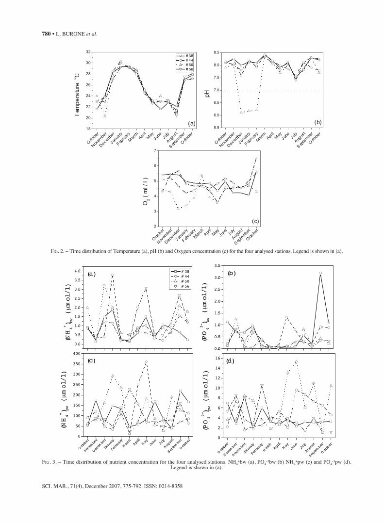
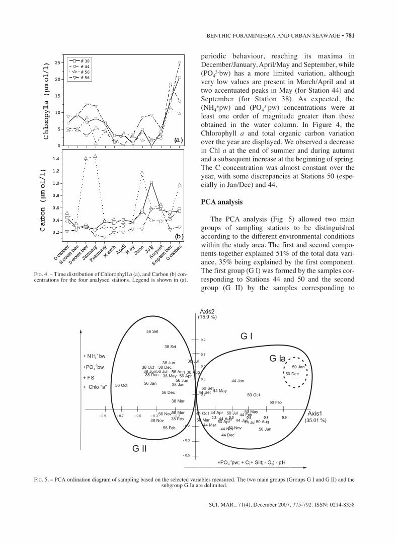
least one order of magnitude greater than thoseobtained in the water column. In Figure 4, theChlorophyll a and total organic carbon variationover the year are displayed. We observed a decreasein Chl a at the end of summer and during autumnand a subsequent increase at the beginning of spring.The C concentration was almost constant over theyear, with some discrepancies at Stations 50 (espe-cially in Jan/Dec) and 44.

PCA analysis

The PCA analysis (Fig. 5) allowed two maingroups of sampling stations to be distinguishedaccording to the different environmental conditionswithin the study area. The first and second compo-nents together explained 51% of the total data vari-ance, 35% being explained by the first component.The first group (G I) was formed by the samples cor-responding to Stations 44 and 50 and the secondgroup (G II) by the samples corresponding to



October

November

December

January

February

MarchAprilMayJune Ju

ly

August

September

October

0.2

0.4

0.6

0.8

1.0

1.2

1.4

(b)

Carbon (

μmol / l )

0

5

10

15

20

25

(a)Chloropyll a (

μmol / l )

# 38 # 44 # 50 # 56

0.2 0.3 0.5 0.7 0.90.2 0.3 0.5 0.7 0.9- 0.2- 0.3- 0.5- 0.7- 0.9

- 0.3

- 0.5

- 0.2

0.2

0.3

0.5

0.7

0.9

50 Jan

50 Dec

50 Oct

44 Jan

44 May50 Set

44 Set

44 Apr 50 Jul44 Oct

50 Mar

44 Mar

44 Aug50 Apr

50 Nov

44 Jun

50 May

50 Aug

50 Jun

56 Set

38 Set

38 Jul

38 Aug56 Aug38 May

38 Jun38 Dec38 Oct

56 Jul38 Jun38 Dec 56 Apr

56 Jun38 Jan56 Jan

56 Dec

56 Oct

38 Mar

56 Mar

38 Feb

56 Nov

38 Nov

56 Feb

G Ia

Axis2

G I

G II

Axis1(35.01 %)

(15.9 %)

+PO pw; + C;4

-3+ Silt; - O ; - pH2

+ N H bw4

+

+PO bw4

-3

+ FS

+ Chlo “a”

50 Feb

44 Feb

44 Nov

44 Dec

44 Jul

FIG. 4. – Time distribution of Chlorophyll a (a), and Carbon (b) con-centrations for the four analysed stations. Legend is shown in (a).

FIG. 5. – PCA ordination diagram of sampling based on the selected variables measured. The two main groups (Groups G I and G II) and the subgroup G Ia are delimited.

Stations 38 and 56. The first one was positivelyrelated to Axis I due to its high concentration of car-bon, silt and (PO4

3-pw), as well as the low oxygencontent and pH values in the bottom water. Withinthis group it was possible to observe a smaller sub-group (G Ia) formed by the months of December andJanuary of Station 50, which had low pH values andO2 content. On the other hand, G II was negativelylinked with Axis I, due to high concentrations of(NH4

+bw), (PO43-bw) and Chl a in the sediment, and

a high fine sand content

Fauna

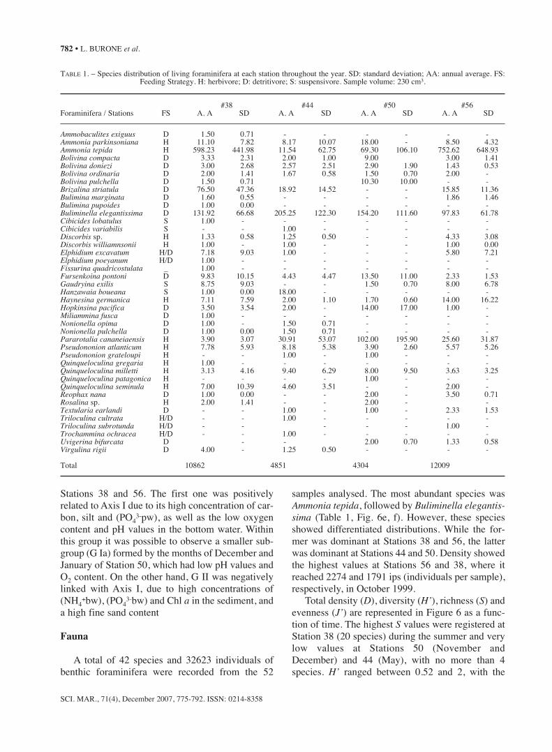
A total of 42 species and 32623 individuals ofbenthic foraminifera were recorded from the 52

samples analysed. The most abundant species wasAmmonia tepida, followed by Buliminella elegantis-sima (Table 1, Fig. 6e, f). However, these speciesshowed differentiated distributions. While the for-mer was dominant at Stations 38 and 56, the latterwas dominant at Stations 44 and 50. Density showedthe highest values at Stations 56 and 38, where itreached 2274 and 1791 ips (individuals per sample),respectively, in October 1999.

Total density (D), diversity (H’), richness (S) andevenness (J’) are represented in Figure 6 as a func-tion of time. The highest S values were registered atStation 38 (20 species) during the summer and verylow values at Stations 50 (November andDecember) and 44 (May), with no more than 4species. H’ ranged between 0.52 and 2, with the



TABLE 1. – Species distribution of living foraminifera at each station throughout the year. SD: standard deviation; AA: annual average. FS: Feeding Strategy. H: herbivore; D: detritivore; S: suspensivore. Sample volume: 230 cm3.

#38 #44 #50 #56Foraminifera / Stations FS A. A SD A. A SD A. A SD A. A SD

Ammobaculites exiguus D 1.50 0.71 - - - - - -Ammonia parkinsoniana H 11.10 7.82 8.17 10.07 18.00 - 8.50 4.32Ammonia tepida H 598.23 441.98 11.54 62.75 69.30 106.10 752.62 648.93Bolivina compacta D 3.33 2.31 2.00 1.00 9.00 3.00 1.41Bolivina doniezi D 3.00 2.68 2.57 2.51 2.90 1.90 1.43 0.53Bolivina ordinaria D 2.00 1.41 1.67 0.58 1.50 0.70 2.00 -Bolivina pulchella D 1.50 0.71 10.30 10.00 - -Brizalina striatula D 76.50 47.36 18.92 14.52 - - 15.85 11.36Bulimina marginata D 1.60 0.55 - - - - 1.86 1.46Bulimina pupoides D 1.00 0.00 - - - - - -Buliminella elegantissima D 131.92 66.68 205.25 122.30 154.20 111.60 97.83 61.78Cibicides lobatulus S 1.00 - - - - - - -Cibicides variabilis S - - 1.00 - - - - -Discorbis sp. H 1.33 0.58 1.25 0.50 - - 4.33 3.08Discorbis williamnsonii H 1.00 - 1.00 - - - 1.00 0.00Elphidium excavatum H/D 7.18 9.03 1.00 - - - 5.80 7.21Elphidium poeyanum H/D 1.00 - - - - - - -Fissurina quadricostulata _ 1.00 - - - - - - -Fursenkoina pontoni D 9.83 10.15 4.43 4.47 13.50 11.00 2.33 1.53Gaudryina exilis S 8.75 9.03 - - 1.50 0.70 8.00 6.78Hanzawaia boueana S 1.00 0.00 18.00 - - - - -Haynesina germanica H 7.11 7.59 2.00 1.10 1.70 0.60 14.00 16.22Hopkinsina pacifica D 3.50 3.54 2.00 - 14.00 17.00 1.00 -Miliammina fusca D 1.00 - - - - - - -Nonionella opima D 1.00 - 1.50 0.71 - - - -Nonionella pulchella D 1.00 0.00 1.50 0.71 - - - -Pararotalia cananeiaensis H 3.90 3.07 30.91 53.07 102.00 195.90 25.60 31.87Pseudononion atlanticum H 7.78 5.93 8.18 5.38 3.90 2.60 5.57 5.26Pseudononion grateloupi H - - 1.00 - 1.00 - - -Quinqueloculina gregaria H 1.00 - - - - - - -Quinqueloculina milletti H 3.13 4.16 9.40 6.29 8.00 9.50 3.63 3.25Quinqueloculina patagonica H - - - - 1.00 - - -Quinqueloculina seminula H 7.00 10.39 4.60 3.51 - - 2.00 -Reophax nana D 1.00 0.00 - - 2.00 - 3.50 0.71Rosalina sp. H 2.00 1.41 - - 2.00 - -Textularia earlandi D - - 1.00 - 1.00 - 2.33 1.53Triloculina cultrata H/D - - 1.00 - - - - -Triloculina subrotunda H/D - - - - - 1.00 -Trochammina ochracea H/D - - 1.00 - - - - -Uvigerina bifurcata D - - 2.00 0.70 1.33 0.58Virgulina rigii D 4.00 - 1.25 0.50 - - - -

Total 10862 4851 4304 12009

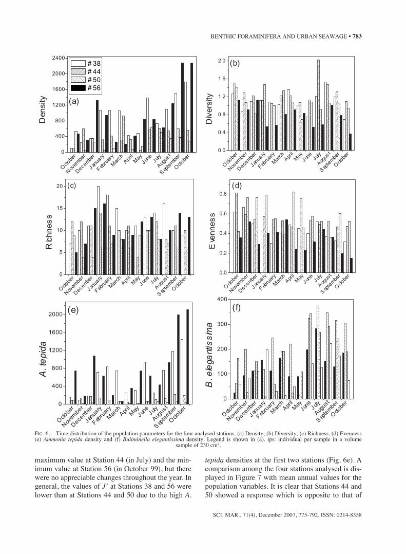
maximum value at Station 44 (in July) and the min-imum value at Station 56 (in October 99), but therewere no appreciable changes throughout the year. Ingeneral, the values of J’ at Stations 38 and 56 werelower than at Stations 44 and 50 due to the high A.

tepida densities at the first two stations (Fig. 6e). Acomparison among the four stations analysed is dis-played in Figure 7 with mean annual values for thepopulation variables. It is clear that Stations 44 and50 showed a response which is opposite to that of



Octo

ber

Nov

embe

r

Dece

mber

Janua

ry

Feb

ruar

y

Mar

chApr

il

May

June

July

Aug

ust

Sep

tembe

r

Octo

ber

0

100

200

300

400

(f)

B. e

lega

ntis

sima

Octo

ber

Nov

embe

r

Dece

mber

Janua

ry

Feb

ruar

y

Mar

chApr

il

May

June

July

Aug

ust

Sep

tembe

r

Octo

ber

0

400

800

1200

1600

2000(e)

A. t

epid

a

Octo

ber

Nov

embe

r

Dece

mber

Janua

ry

Feb

ruar

y

Mar

chApr

il

May

June

July

Aug

ust

Sep

tembe

r

Octo

ber

0.0

0.2

0.4

0.6

0.8

(d)

Eve

nn

es

s

Octo

ber

Nov

embe

r

Dece

mber

Janua

ry

Feb

ruar

y

Mar

chApr

il

May

June

July

Aug

ust

Sep

tembe

r

Octo

ber

0

5

10

15

20 (c)

Rich

nes

s

Octo

ber

Nov

embe

r

Dece

mber

Janua

ry

Feb

ruar

y

Mar

chApr

il

May

June

July

Aug

ust

Sep

tembe

r

Octo

ber

0.0

0.4

0.8

1.2

1.6

2.0 (b)

Div

ers

ity

Octo

ber

Nov

embe

r

Dece

mber

Janua

ry

Feb

ruar

y

Mar

chApr

il

May

June

July

Aug

ust

Sep

tembe

r

Octo

ber

0

400

800

1200

1600

2000

2400

(a)

Den

sity

# 38

# 44

# 50

# 56

FIG. 6. – Time distribution of the population parameters for the four analysed stations. (a) Density; (b) Diversity; (c) Richness, (d) Evenness(e) Ammonia tepida density and (f) Buliminella elegantissima density. Legend is shown in (a). ips: individual per sample in a volume

sample of 230 cm3.

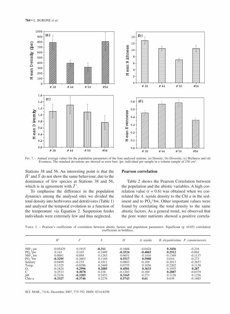
Stations 38 and 56. An interesting point is that theH–’ and S– do not show the same behaviour, due to thedominance of few species at Stations 38 and 56,which is in agreement with J–’.

To emphasise the difference in the populationdynamics among the analysed sites we divided thetotal density into herbivores and detritivores (Table 1)and analysed the temporal evolution as a function ofthe temperature via Equation 2. Suspension feederindividuals were extremely few and thus neglected.

Pearson correlation

Table 2 shows the Pearson Correlation betweenthe population and the abiotic variables. A high cor-relation value (r = 0.6) was obtained when we cor-related the A. tepida density to the Chl a in the sed-iment and to PO4

3-bw. Other important values werefound by correlating the total density to the sameabiotic factors. As a general trend, we observed thatthe pore water nutrients showed a positive correla-



# 38 # 44 # 50 #560

100

200

300

400

500

600

700

800

900

1000(a)

Mean Density (ips)

# 38 # 44 # 50 #560

2

4

6

8

10

12

14 (b)

Mean Richness

# 38 # 44 # 50 #560.0

0.2

0.4

0.6

0.8

1.0

1.2

1.4

1.6(c)

Mean Diversity

# 38 # 44 # 50 #560.0

0.1

0.2

0.3

0.4

0.5

0.6 (d)

Mean Evenness

FIG. 7. – Annual average values for the population parameters of the four analysed stations. (a) Density; (b) Diversity; (c) Richness and (d) Evenness. The standard deviations are showed as error bars. ips: individual per sample in a volume sample of 230 cm3.

TABLE 2. – Pearson’s coefficients of correlation between abiotic factors and population parameters. Significant (p <0.05) correlation coefficients in boldface.

H’ J’ S D A. tepida B. elegantissima P. cananeiaensis

NH+4 pw -0.05429 0.1915 -0.311 -0.1668 -0.0424 0.3456 -0.216

PO4-3pw 0.143 0.165 -0.2489 -0.3524 -0.4065 0.2912 -0.004

NH+4 bw -0.0681 -0.094 0.1263 0.0651 0.1416 -0.1369 -0.1137

PO4-3bw -0.3295 -0.2603 0.1169 0.5517 0.5988 0.016 -0.273

Salinity -0.0499 -0.155 0.1911 0.0803 -0.189 -0.2013 -0.2657Temp. 0.1325 -0.0296 0.2469 0.0755 0.1056 -0.2202 0.1138O2 -0.1824 0.2996 0.2885 0.4501 0.3633 0.1955 0.287C 0.2513 0.3078 -0.238 -0.1203 -0.189 0.2887 -0.0379pH -0.2336 -0.3205 0.2452 0.3165 0.273 0.1128 0.1226Chlo a -0.3327 -0.3746 0.2276 0.5743 0.61 0.039 -0.1885

tion with B. elegantissima, whereas PO43-bw was

positively correlated with A. tepida. A. tepida wasdominant at Stations 38 and 56, while B. elegantis-sima was dominant at Stations 44 and 50.

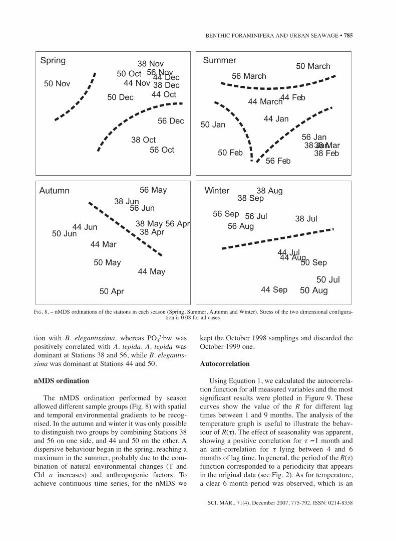
nMDS ordination

The nMDS ordination performed by seasonallowed different sample groups (Fig. 8) with spatialand temporal environmental gradients to be recog-nised. In the autumn and winter it was only possibleto distinguish two groups by combining Stations 38and 56 on one side, and 44 and 50 on the other. Adispersive behaviour began in the spring, reaching amaximum in the summer, probably due to the com-bination of natural environmental changes (T andChl a increases) and anthropogenic factors. Toachieve continuous time series, for the nMDS we

kept the October 1998 samplings and discarded theOctober 1999 one.

Autocorrelation

Using Equation 1, we calculated the autocorrela-tion function for all measured variables and the mostsignificant results were plotted in Figure 9. Thesecurves show the value of the R for different lagtimes between 1 and 9 months. The analysis of thetemperature graph is useful to illustrate the behav-iour of R(τ). The effect of seasonality was apparent,showing a positive correlation for τ =1 month andan anti-correlation for τ lying between 4 and 6months of lag time. In general, the period of the R(τ)function corresponded to a periodicity that appearsin the original data (see Fig. 2). As for temperature,a clear 6-month period was observed, which is an



50 Nov

38 Nov56 Nov50 Oct 44 Dec

38 Dec44 Nov

44 Oct50 Dec

56 Dec

38 Oct

56 Oct

Spring Summer50 March

56 March

44 Feb44 March

44 Jan50 Jan

50 Feb

56 Jan38 Jan38 Mar

38 Feb56 Feb

Autumn 56 May

38 Jun56 Jun

38 May 56 Apr38 Apr

44 Jun50 Jun

44 Mar

50 May44 May

50 Apr

Winter 38 Aug38 Sep

56 Sep 56 Jul

56 Aug38 Jul

44 Jul44 Aug

50 Sep

50 Jul

50 Aug44 Sep

FIG. 8. – nMDS ordinations of the stations in each season (Spring, Summer, Autumn and Winter). Stress of the two dimensional configura-tion is 0.08 for all cases.

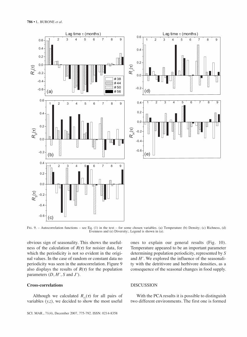
obvious sign of seasonality. This shows the useful-ness of the calculation of R(τ) for noisier data, forwhich the periodicity is not so evident in the origi-nal values. In the case of random or constant data noperiodicity was seen in the autocorrelation. Figure 9also displays the results of R(τ) for the populationparameters (D, H’, S and J’).

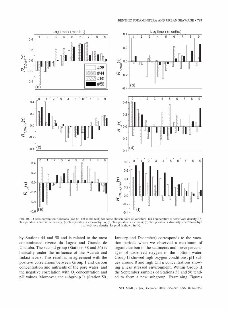
Cross-correlations

Although we calculated Ryz(τ) for all pairs ofvariables (y,z), we decided to show the most useful

ones to explain our general results (Fig. 10).Temperature appeared to be an important parameterdetermining population periodicity, represented by Sand H’. We explored the influence of the seasonali-ty with the detritivore and herbivore densities, as aconsequence of the seasonal changes in food supply.

DISCUSSION

With the PCA results it is possible to distinguishtwo different environments. The first one is formed



-0.6

-0.4

-0.2

0.0

0.2

0.4 1 2 3 4 5 6 7 8 9

(e)

RH

’(τ)

-0.2

0.0

0.2

0.4

0.61 2 3 4 5 6 7 8 9

(d)

RJ’(τ)

-0.6

-0.4

-0.2

0.0

0.2

0.41 2 3 4 5 6 7 8 9

(c)

RS(τ)

-0.2

0.0

0.2

0.4

0.61 2 3 4 5 6 7 8 9

(b)

RD( τ)

-0.6

-0.4

-0.2

0.0

0.2

0.4

0.6 1 2 3 4 5 6 7 8 9

(a)

Lag time τ (months) Lag time τ (months)R

T(τ)

# 38

# 44

# 50

# 56

FIG. 9. – Autocorrelation functions – see Eq. (1) in the text – for some chosen variables. (a) Temperature (b) Density; (c) Richness, (d) Evenness and (e) Diversity;. Legend is shown in (a).

by Stations 44 and 50 and is related to the mostcontaminated rivers: da Lagoa and Grande deUbatuba. The second group (Stations 38 and 56) isbasically under the influence of the Acaraú andIndaiá rivers. This result is in agreement with thepositive correlations between Group I and carbonconcentration and nutrients of the pore water; andthe negative correlation with O2 concentration andpH values. Moreover, the subgroup Ia (Station 50,

January and December) corresponds to the vaca-tion periods when we observed a maximum oforganic carbon in the sediments and lower percent-ages of dissolved oxygen in the bottom water.Group II showed high oxygen conditions, pH val-ues around 8 and high Chl a concentrations show-ing a less stressed environment. Within Group IIthe September samples of Stations 38 and 56 tend-ed to form a new subgroup. Examining Figures



-0.4

-0.2

0.0

0.2

0.4

0.6

0.8 0 1 2 3 4 5 6 7 8 9

(f)

(R

Chlo

a,H

erbτ)

-0.6

-0.4

-0.2

0.0

0.2

0.40 1 2 3 4 5 6 7 8 9

(e)

RT

,H’( τ)

-0.4

-0.2

0.0

0.2

0.4

0 1 2 3 4 5 6 7 8 9

(d)

R

T,S(τ)

-0.4

-0.2

0.0

0.2

0.40 1 2 3 4 5 6 7 8 9

(c)

RT

,Chlo

’a’(τ)

-0.4

-0.2

0.0

0.2

0.41 2 3 4 5 6 7 8 9

Lag time τ (months)

(b)

R

T,H

erb(

τ)

-0.4

-0.2

0.0

0.2

0.41 2 3 4 5 6 7 8 9

(a)

Lag time τ (months)

R

T,D

etri(

τ)

#38

#44

#50

#56

FIG. 10. – Cross-correlation functions (see Eq. (2) in the text) for some chosen pairs of variables. (a) Temperature x detritivore density; (b)Temperature x herbivore density; (c) Temperature x chlorophyll a; (d) Temperature x richness; (e) Temperature x diversity; (f) Chlorophyll

a x herbivore density. Legend is shown in (a).

3(a) and (b), we see an NH4+bw peak for Station 56

and a PO43-bw peak for Station 38, followed by a

general increase in Chl a, which is also noted in thelocation of the September samples of Stations 44and 50 in Group I. Furthermore, a considerableincrease in total foraminiferal density wasobserved at Stations 38 and 56. An interestingpoint is that Group I was basically dominated bydetritivore species (especially B. elegantissima, seeTable 1), probably due to carbon and pore waterphosphate enrichment, which was an importantcontribution in the first eigenvalue of PCA (axis I).Similarly, Group II was mostly populated by herbi-vore species (especially A. tepida, Murray (1991)),whereas the PCA showed a positive correlationwith Chl a and column water nutrients. The totalforaminiferal densities were in agreement with thissegregation, since Group II was much more popu-lated than Group I, which revealed the most stress-ful conditions.

Seasonally, the nMDS analysis segregated thestations into two or three main groups according tothe composition of the fauna throughout the studiedyear (see Fig. 8). This ordination analysis indicateda seasonal change in the station grouping based onforaminiferal distribution. A fairly homogeneousstation group appeared in the autumn/winter period.It is also possible to observe two group separationsthat are very similar to that seen in the PCA. A sig-nificant change appeared in the spring period. TheStation 50 in November is almost azoic, appearingisolated in the diagram. On the opposite diagonalside a group of three samples that are dominated byA. tepida can be seen. The middle group showed amore homogeneous species distribution. In summerthe nMDS diagram dispersion was quite evident.The January and February samples at Station 50showed very low densities, possibly as a conse-quence of low pH and O2 concentrations as well asthe high NH4

+ concentration in the pore water.According to Bricker et al. (2003), O2 concentra-tions >1.4 and ≤3.5 ml/L-1 may cause biologicalstress. Thus, the simultaneous action of these abiot-ic factors probably makes the environment inhos-pitable for foraminiferal fauna development. On theother side of the diagram, the samples of Stations 50and 56 of March share local blooms of Pararotaliacananeiaensis, positively correlated to the O2 con-centration (see Fig. 2c and Table 2). All of theseaspects are evidence of the rapid foraminiferalresponse to the abiotic disturbances.

As a rule, Stations 38 and 56 showed the highestdensities of foraminifera, represented basically byhyaline species and dominated by Ammonia tepida.The high density of A. tepida is consistent with theresults of other authors, who have pointed out itsability to tolerate lower salinities (Walton and Sloan,1990). Debenay et al. (2001) stated that the growthof this species may be favoured by a temporarydecrease in water salinity and by input of nutrients,which are both clearly observed at these stations(Table 1, Fig. 6e). Nevertheless, in this case, the lowsalinity is similar for all sites, and may not be usedto justify the different distribution among the fourstudied sites. It is known that an increase in nutrientconcentrations usually implies in an increase in pri-mary producers, which results in an important feed-ing source for herbivore foraminiferal fauna, such asA. tepida (Erskian and Lipps, 1987; Murray andAlve, 2000). A positive correlation between A. tepi-da densities and Chl a concentration was shown bythe Pearson correlation (0.61, see Table 2).According to Hohenegger et al (1989), A. tepidashows a strong preference for Cyanobacteria andavoids certain abundant diatoms. Similarly, a posi-tive correlation was also observed in the cross-cor-relation RChlo a,Herbivores(τ) at Stations 38, 44 and 56for lag times of at least 3 months. In contrast, Station50 was dominated by detritivore species, whichexplains its negative RChlo a,Herbivores(τ) coefficient.

Stations 44 and 50 contained mainly hyalinespecies, Buliminella elegantissima being the domi-nant one. However, other contributions of aggluti-nant and porcelanaceous species were also found. B.elegantissima showed a positive correlation withcarbon concentration and nutrient pore water con-centrations, indicating their preference for organicenriched environmental conditions, similarly to theobservations of Setty (1982), Murray (1991) Bonetti(2000), and Burone and Pires-Vanin (2006).

Figure 7 represents the mean annual behaviour ofthe analysed stations. Stations 38 and 56 showedlow diversity and evenness values, which are close-ly related to the A. tepida dominance. Although thisdominance appears to be almost constant year-round, there are a few A. tepida peaks (strongly con-tributing to D, see Figure 6 and Table 1) that werelinked to Chl a maximum concentrations. Althoughwe noticed the presence of juvenile individualsthroughout the year, their presence increased inmonths of higher temperature, which is in agree-ment with former observations (Jones and Ross,



1979). All these features may be seen as a result ofa high adaptability of A. tepida to survive in underunstable environments.

An interesting point is the fact that the meandiversity (Fig. 7) is approximately homogeneousamong all sites, and Stations 44 and 50 showedslightly higher mean diversity values than Stations38 and 56, despite their low densities. In fact, forStation 50 the density would be even lower if it werenot for a P. cananeiaensis peak in March. In thiscase, the high diversity does not lead to a healthyenvironment, since the extremely low foraminiferaldensities demonstrate harmful conditions for faunareproduction and growth. Actually, there were fewmoments with fewer than 50 individuals at Station50. The H’ index must therefore be used with care,because a sample with just a few individuals equal-ly distributed among few species has higher diversi-ty than a sample with many individuals of only onespecies, but the latter may be more appropriate forreproduction and growth (Burone et al. 2006). Thus,there is a major difference between the living domi-nant species of these two pairs of stations: Stations38-56 with the herbivore A. tepida and Stations 44-50 with the detritivore B. elegantissima. This evi-dences the organic enrichment at Stations 44 and 50.Furthermore, the abiotic factors measured also indi-cate higher anthropogenic contamination at Stations44 and 50 (see Fig. 5). These results are in agree-ment with Pearson and Rosenberg (1978), whoobserved that an excess supply of organic materialmay lead to a collapse of the benthic community.Most investigations have reported the presence of anazoic zone or an area with extremely low abundanceas a consequence of low oxygen and pH values(Clark, 1971; Boltovskoy and Wright, 1976; Alve,1995). In the literature, A. tepida and B. elegantissi-ma are considered resistant or tolerant to the pollu-tants (see for example Yanko et al., 1999). Ourresults show that B. elegantissima is more resistantthan A. tepida, indicating the spatial distribution ofboth dominant species.

We decided to calculate the cross-correlationfunction for T since it is a strong parameter thatvaries equally in time for all stations, so any differ-ences in the population responses among the stationsmust be attributed to other factors. In Figure 10(a) aseasonal behaviour of the detritivore density is clearfor all stations. We observe a negative maximum forsmall lag times and a positive maximum for a lagtime around 6 months. This is probably due to the

time needed for organic matter to decompose. Thebehaviour is almost opposite to that of herbivores,shown in Figure 10(b), but in this case the seasonali-ty is not so evident for all stations. As for Station 38,a periodicity of approximately 5 months is clear, butwith an opposite phase. The strong positive maxi-mum for τ = 0 means that an increase in T leads to anincrease in the herbivore species density at the sametime. This is a clear consequence of the Chl aincrease, as seen in Figure 10(c), which shows thecross-correlation between T x Chl a, demonstrating aclear periodicity of approximately 6 months, verysimilar to Figure 10(b). As expected, the Chl a fol-lows temperature changes, as a consequence of lightincidence. In the specific case of Ubatuba Bay, theincrease in T is concomitant to the vacation period,and consequently to an increase in nutrients comingfrom the rivers, which stimulate phytoplanktonorganisms. A similar response of the RT,Chlo a(τ) andRT,Herb(τ) observed at Station 38 would be expected innon-stressed environments. At Station 56 the behav-iour is approximately the same, but the correlationsare not so strong. Although this station is more con-fined and the Indaiá River is not so polluted, the bay’sclockwise water circulation may transport contami-nants from the other rivers. Nevertheless, Stations 44and 50 do not show a clear response to temperature(or to Chl a), due basically to the low-density popu-lations and high environmental instability.

Richness and diversity are also closely connect-ed to temperature. In general, regions close to theequator show higher diversity and number of speciesthan the poles (Odum, 1972). However, in ananthropogenic-affected environment this effect maybe masked. Furthermore, in micro-ecosystem analy-sis it is not possible to infer strong correlationsbetween T and S, and other factors must be takeninto account. In Figures 10(d) and (e) it is seen thatRT,S(τ) and RT,H’(τ) have an opposite phase for all sta-tions. Stations 38, 44 and 56 have a positive maxi-mum for τ≅0 in the RT,S(τ) curve, whereas Station 50has a negative maximum. Once more, Stations 38and 56 show a more evident seasonal pattern (of 4 or6 months), whereas Stations 44 and 50 show differ-ent responses to their stressing conditions, such asvery low pH and O2 content. The response of diver-sity to temperature occurs with the opposite phase,which is a consequence of the dominance of A. tep-ida and B. elegantissima. These results for the timeresponse analysis are in agreement with the meanannual results discussed above.



Completing our temporal analysis, we brieflydiscuss the results of the autocorrelation coefficientfor T, D, S, J’ and H’. Usually, for a good time seriesanalysis an observation time much longer than theperiod one wants to analyse is necessary. This con-dition implies a high statistical significance for alllag times within the period analysed. Unfortunately,our data set extends for just one year, which limitsour precision for high lag times. However, in caseswhere the observed data oscillate rapidly, it is possi-ble to distinguish periods of the order of 2 to 6months even in a short set of data such as ours. Aspointed out above, the 6-month period of RT(τ) isevidence of the periodic behaviour of the originaldata, basically due to seasonality. As seen in theother curves, no periodicity is found for the popula-tion parameters. This is due to the many differentabiotic parameters that are not correlated in time,and are acting on the foraminiferal fauna. It must beemphasised that non-periodic does not mean ran-dom, but simply a result of the out-of-phase inputsof the abiotic components.

CONCLUSIONS

In this work we have studied benthicforaminiferal variability over a period of thirteenmonths at four coastal stations, each of which isbasically influenced by one river. Geochemical andpopulation parameters allowed the sites to be sepa-rated into two groups according to their degree ofstress. Stations 38 and 56 were the most productive,having higher densities, with a high dominance of A.tepida and less stressful chemical conditions. Thesefeatures are a consequence of the nutrient enrich-ment from the less polluted rivers. The Acaraú andIndaiá Rivers do not cross the urban zone and arenot strongly affected by sewage. The high densityobserved at these stations is a biological effect thatis in agreement with previous studies on the influ-ence of domestic waste and organic enrichment onthe benthic foraminiferal population (Yanko et al.,1994; Samir and El-Din, 2001; Burone et. al., 2006).On the other hand, Stations 44 and 50 are less pro-ductive, having almost azoic moments, and are dom-inated by B. elegantissima, which is typical oforganic-enriched environments.

At Station 50, the low oxygen concentrations andpH values provide a high-stressed zone for the biotaestablishment. The low population density at

Stations 44 and 50 near the da Lagoa and Grande deUbatuba Rivers may be correlated to the rivers’water quality. The excess of organic matter andnutrients makes the environment uninhabitable formost foraminiferal species. As a natural conse-quence of organic matter degradation, the O2 rateconsumption and acidification are high. As a gener-al comparison, it was possible to identify thatStation 38 is less affected by environmental stress.This is due to its strong marine influence, since thewater circulation is clockwise and the Acaraú Riveris the least polluted one.

The dominance of Ammonia tepida at Stations 38and 56 is closely related to food abundance, asreflected in the Chl a content. In our study area, A.tepida did not show resistance to low O2 concentra-tions and extremely acid pH values. B. elegantissi-ma appeared as an opportunist species at Stations 44and 50, since it is naturally infaunal and detritivore,occupying the niche left by A. tepida. Although A.tepida and B. elegantissima are considered resistantto contamination, B. elegantissima appears to bemore opportunistic or resistant. A confirmation ofthese hypotheses will come from core analysis forthe same sites, which have been made and will bethe subject of further work.

As seen in the annual average values, the speciesdiversity did not seem to be a good indicator of envi-ronmental health in places with high dominances orlow densities, but density and richness could be usedas evidence of local productivity and environmentalconditions. The annual average results for the popu-lation parameters showed an interesting discrepancybetween richness and diversity, a consequence ofoccasional dominance of some opportunist species(e.g. A tepida and B. elegantissima), which wouldnot be observed in a single field sampling. It isimportant to note that the lack of replicate samplescould affect some interpretations concerning the dif-ferences among locations, since the replicates couldsmooth over possible patches in foraminiferal distri-bution.

The annual monitoring showed that the anthro-pogenic effect is stronger in the austral summer peri-od, when there is a massive increase in tourism, sothe sewage input by the rivers in the Ubatuba Bayalso increases.

It is clear that our results support the importanceof time series analysis. The use of the cross-correla-tion seems to be a good tool for analysing the influ-ence of abiotic parameters on the temporal evolution



of the foraminiferal fauna. Thus, this mathematicaltool complements other statistical analysis, likenMDS and PCA, bestowing more attention on sea-sonal environmental changes and the consequentseasonal biotic response. Thus, it is important forfuture monitoring work to extend through periodslonger than a single year. A possible future utilisa-tion of the cross-correlation function lies in theanalysis of the influence of the water circulationupon the foraminiferal population dynamics, sincethe contribution of one river may affect not only itscorresponding station, but others as well if sometime interval is considered.

ACKNOWLEDGEMENTS

This work was supported by the Fundação deAmparo à Pesquisa do Estado de São Paulo (FAPE-SP, Brazilian agency) through a doctoral fellowship(Proc. N° 97/12493-7) provided to L.B. Thanks areextended to the Oceanographic Institute of theUniversity of São Paulo for providing field and lab-oratory facilities.

REFERENCES

Abessa, D.M de S. and L. Burone. – 2003. Toxicity of sedimentsfrom the rivers situated in Ubatuba Bay (SP, Brazil). O Mundoda Saúde. 27(4): 564-569.

Alve, E. – 1991. Benthic foraminifera reflecting heavy metal pollu-tion in Sorjord, Western Norway. J. Foraminifer. Res., 34:1641-1652.

Alve, E. – 1995. Benthic foraminifera response to estuarine pollu-tion. A review. J. Foraminifer. Res., 25 (3): 190-203.

Armynot Du Châtelet, E., J-P. Debenay and R. Soulard. – 2004.Foraminiferal proxies for pollution monitoring in moderatelypolluted harbors. Mar. Pollut. Bull., 127: 27-40.

Boltovskoy, E., D.B Scott and F.S. Medioli. – 1991. Morphologicalvariations of benthic foraminiferal test in response to changes inecological parameters: a review. J. Paleontol., 65(2): 175- 185.

Boltovskoy, E. and R. Wright. – 1976. Recent Foraminífera. W.Junk (ed) The Hague.

Bonetti, C. – 2000. Foraminíferos como bioindicadores do gradi-ente de estresse ecológico em ambientes costeiros poluídos.Estudo aplicado ao sistema astuarino de Santos-São Vicente(SP, Brasil). Ph. D. thesis, Instituto Oceanográfico, Univ. deSão Paulo, São Paulo.

Bray, J.R. and J. T. Curtis. – 1957. An ordination of the upland for-est communities in southern Wisconsin. Ecol. Monogr., 27:325-349.

Bricker, S.B., J.G. Ferreira and T. Simas. – 2003. An integratedmethodology for assessment of estuarine trophic status. Ecol.Model. 169: 39-60.

Burone, L., 2002. Foraminíferos Bentônicos e Parâmetros físico-químicos da Enseada de Ubatuba, São Paulo: EstudoEcológico em uma área com Poluição Orgânica. Ph. D thesis,Instituto Oceanográfico, Univ. de São Paulo, São Paulo.

Burone, L., E. Braga, P. Valente and A.M.S. Pires-Vanin. – 2005.A Chemical Analysis of sediment pore water in oxygen-freeatmosphere: application to a contaminated area. Braz. J.Oceanogr. 53(1-2): 69-74.

Burone, L., P. Muniz, A.M.S. Pires-Vanin and M. Rodrigues. –2003. Spatial distribution of organic matter in the surface sedi-ments of Ubatuba Bay (Southeastern - Brazil). An. Acad. Bras.Ciênc. 75(1): 1-14.

Burone, L. and A.M. S. Pires-Vanin. – 2006. Foraminiferal assem-blages in the Ubatuba Bay, Southeastern Brazilian coast. Sci.Mar., 70(2): 203-217.

Burone, L., N. Venturini, P. Sprechmann, P. Valente and P. Muniz. –2006. Foraminiferal responses to polluted sediments in theMontevideo coastal zone, Uruguay. Mar. Pollut. Bull. 52: 61-73.

CETESB (Companhia de Tecnologia de Saneamento Ambiental). –1996. Relatório de Balneabilidade das Praias Paulistas, 1995.Secretaria do Meio Ambiente, São Paulo, Brazil.

CETESB (Companhia de Tecnologia de Saneamento Ambiental). –2000. Relatório de Balneabilidade das Praias Paulistas, 1999.Secretaria do Meio Ambiente, São Paulo, Brazil.

Clark, D.F. – 1971. Effects of aquaculture outfall on benthonicforaminifera in Clam Bay, Nova Scotia: Marit. Sedim., 7: 76-84.

Clarke K.R. and R.M. Warwick. – 2001. Change in marine com-munities: an approach to statistical analysis and interpretation.Plymouth Marine Laboratory, Plymouth.

Debenay, J.P., E. Geslin, B.B. Eichler, W. Duleba, F. Sylvestre andP. Eichler. – 2001. Foraminiferal assemblages in a hypersalinelagoon Araruama (RJ) Brazil. J. Foraminifer. Res., 31(2): 133-151.

Erskian, M.G. and J.U.H. Lipps.- 1987. Population dynamics of theforaminiferan Glabratella ornatissima (Cushman) in northernCalifornia: J. Foraminifer. Res., 17: 240-256.

Grasshoff, K., M. Ehrhardt and K.V. Kremeling. – 1983. Methodsof seawater analysis. Verlag Chemie, Weinheim.

Hohenegger, J., W. Piller and C. Baal. – 1989. Reasons for spatialmicrodistributions of foraminifers in an intertidal pool(Northern Adriatic Sea). Mar. Ecol., 10(1): 43-78.

Jones, G.D. and C.A. Ross. – 1979. Seasonal distribution offoraminifera in Samish Bay, Washington. J. Paleont., 53:245- 257.

Jorgensen, B. – 1996. Material flux in the sediment. In: Coastal andestuarine studies, (ed.), By B. Jorgensen and K. Richardson.American Geophysical Union.

Kovach, W.L. – 1999. MVSP – A multivariate statistical packagefor windows, ver. 3.1. Kovach Computing Services, Pentraeth,Wales.

Kruskal, J.B. and M. Wish. 1978. Multidimensional scaling.California Sage, Beverly Hills.

Loeblich, A.R. and H. Tappan. 1988. Foraminiferal Genera andtheir Classification: Van Nostrand Reinhold, New York.

Lorenzen, C.J. – 1967. Determination of chlorophyll and pheopig-ments: Spectrofotometric equations. Limnol. Oceanogr., 12:343- 346.

Mahiques, M.M., M.G. Tessler and V.V. Furtado. – 1998.Characterization of energy gradient in enclosed bays ofUbatuba region, South-eastern, Brazil. Est. Coast. Shelf Sci.,47: 431-446.

Muniz, P. – 2003. Comunidades macrobênticas como indicadorasda qualidade ambiental de ecossistemas costeiros rasos: estu-do de caso – Enseada de Ubatuba (SP, Brasil). Ph. D. thesis,Instituto Oceanográfico, Univ. de São Paulo, São Paulo.

Murray, J.W. – 1991. Ecology and Paleoecology of BenthicForaminifera. Longman, Harlow.

Murray, J.W. and E. Alve. – 2000. Major aspects of foraminiferalvariability (standing crop and biomass) on a monthly scale in anintertidal zone. J. Foraminifer. Res., 30 (3): 177-191.

Odum, E.P. – 1972. Ecología. Editora Nueva EditorialInteramericana, S. A., México.

Pearson, T.H. and R. Rosenberg. – 1978. Macrobenthic successionin relation to organic enrichment and pollution of marine envi-ronment. Oceanogr. Mar. Biol Annu Rev., 16: 229-311.

Pielou, E.C. – 1975. Ecological diversity. John Wiley, New York.Reisig, J.M. – 1960. Foraminiferal ecology around ocean outfalls

off southern California. Waste Disposal in the MarineEnvironment. Pergamon Press. London.

Samir, A.M. and A.B. El-Din. – 2001. Benthic foraminiferal assem-blages and morphological abnormalities as pollution proxies intwo Egyptian bays. Mar. Micropaleontol., 41: 193-227.

Scott, D.B., F.S. Medioli, C.T. Shafer. – 2001. Monitoring ofCoastal environments using Foraminifera and Thecamoebianindicators. Cambridge University Press.



Setty, M.G.A.P. – 1982. Pollution effects monitoring withforaminifera as indices in the Thana Creek, Bombay area:Indian J. Mar. Sci., 18: 205-209.

Shannon, C.E. and W.W. Weaver. – 1963. The mathematical theo-ry of communication. University of Illinois Press, Urbana.

Strickland, J.D.H. and T.R. Parsons. – 1968. A practical handbook ofsea-water analysis. Bull. Fish. Res., Board, Canada., 169: 1-311.

Suguio, K. – 1973. Introdução à sedimentologia. São Paulo, EdgarBlücher/ Editora da Universidade de São Paulo (EDUSP).

Tréguer, P. and P. Le Corre. – 1975. Manuel d’ analysis des selsnutritifs dans l’eau de mer. 2ème éd. Brest, Université deBretagne Occidentale.

Turner, S.J., S.F. Thrush, R.D. Pridmore, J.E. Hewitt, V.J.Cummings, and M. Maskery. – 1995. Are soft-sediment com-munities stable? An example from a windy harbour. Mar. Ecol.Prog. Ser., 120: 219-230.

Walton, W.R. – 1952. Techniques for recognition of livingforaminifera. Contrib. Cushman Found. Foram. Res., 3: 56-60.

Walton, W.R. and B. Sloan. – 1990. The genus Ammonia Brünnich.1972: its geographic distribution and morphological variability.

J. Foraminif. Res., 20: 128-156.Watkins, J.G. – 1961. Foraminiferal ecology around the Orange

County, California, ocean sewer outfall. Micropaleontology, 7:199-206.

Wilson, B. and R.A. Dawe. – 2006. Detecting seasonality usingtime series analysis: comparing foraminiferal populationdynamics with rainfall data. J. Foraminif. Res., 36:108-115.

Yanko, V., A. Arnold and W. Parker. – 1999. Effect of marine pol-lution on benthic foraminifera. In: B.K. Sen Gupta (ed.),Modern Foraminifera, pp. 217-235. Kluwer AcademicPublishers, Dordrecht.

Yanko, V., J. Kronfeld and A. Flexer. – 1994. Response of benthicforaminifera to various pollution sources: implications for pol-lution monitoring. J. Foraminif. Res., 24(1): 1-17.

Zalesny, E.R. – 1959. Foraminiferal ecology of Santa Monica Bay.California. Micropaleontology, 5: 101- 126.

Scient. ed.: M.P. Olivar.Received February 12, 2007. Accepted September 3, 2007.Published online November 9, 2007.



Estudio de foraminífiros bentónicos en escala mensual en una bahía subtropical moderadamente afectada por efluentes urbanos

Documents