Estuarine, Coastal and Shelf Scienceweb.iitd.ac.in/~adrao/publications/2016_3.pdf · 27 October 2016 Accepted 28 October ... One of the unique features of the BoB is the different

lable at ScienceDirect

Estuarine, Coastal and Shelf Science 184 (2017) 21e29

Contents lists avai

Estuarine, Coastal and Shelf Science

journal homepage: www.elsevier .com/locate/ecss

Redistribution of low-salinity pools off east coast of India duringsouthwest monsoon season

D.K. Mahapatra a, *, A.D. Rao b

a National Centre for Medium Range Weather Forecasting, Ministry of Earth Sciences, A-50, Institutional Area, Sector-62, Noida 201309, Uttar Pradesh, Indiab Centre for Atmospheric Sciences, Indian Institute of Technology Delhi, Hauz Khas, New Delhi 110 016, India

a r t i c l e i n f o

Article history:Received 2 January 2014Received in revised form27 October 2016Accepted 28 October 2016Available online 31 October 2016

Keywords:Ocean currentsOcean circulationWaterSaline intrusionJets

* Corresponding author.E-mail address: [email protected] (D.K. Mahap

http://dx.doi.org/10.1016/j.ecss.2016.10.0370272-7714/© 2016 Elsevier Ltd. All rights reserved.

a b s t r a c t

The east coast of India receives significant inputs of fresh water into the Bay of Bengal during thesouthwest monsoon in comparison with the lower influx seen on the west coast. However, in situ ob-servations made off the east coast suggest that in some years low-salinity pools appear offshore, asopposed to where the river discharge actually takes place. To date, no studies have offered any plausiblereason for this anomaly. In an attempt to understand the processes involved, we used numericalmodelling to elucidate the causes and mechanisms underlying the appearance of offshore low salinitypools. The model uses temperature and salinity information from the World Ocean Atlas 2001 as initialconditions, and is forced using wind stress derived from the weekly wind for July 2002 and 2010 fromthe NCEP FNL Operational Global Analysis, because of the need to validate the model using more recentobservations. It was found that the formation of a low-salinity pool to the south of 16�N and its migrationto an offshore region is a result of (i) coastal orientation, (ii) surface circulation supported by a weak EastIndia Coastal Current that redistributes fresh water from two rivers, the Krishna and Godavari, and (iii) aninflux of low salinity from the much larger river system to the north, resulting in anomalous pool(s) oflow-salinity waters away from the coast. These findings are corroborated by CTD data, ARGO data, andOcean Surface Current Analysis Real-Time currents.

© 2016 Elsevier Ltd. All rights reserved.

1. Introduction

The Indian Ocean differs from the Atlantic and the Pacific in itslimited northward extent to only 25�N.With its unique exposure tothe monsoons, it represents an area of marked seasonal variability.The essential parts of the North Indian Ocean (NIO) are the ArabianSea in the west and the Bay of Bengal (BoB) in the east. Although,the two are bound by nearly the same latitudes, they have verydistinct basic characteristics. The BoB has significantly low-salinities because all major rivers in India discharge here andconsequently, is distinguished by strong near-surface stratification.The seasonally reversing winds, together with the freshwater gainduring the SW monsoon and the intense air-sea interaction,particularly; during the depression or cyclone development stages,make up the basic physical forcing that brings about large spatialand temporal variations of the surface waters that regulate theupper ocean circulation and the ensuing temperature and salinity

atra).

fields. Differential distribution of salinity and temperature inducehorizontal pressure gradients that alter the circulation. The ArabianSea, on the other hand, is an area of high evaporation that receiveslittle freshwater from the continental land mass and hence, is moresaline.

The wind stress has a direct bearing on the upper layers of theocean. It is, therefore, pertinent here to have an overview of thewind field, the physical processes, and circulation during the pre-monsoon and monsoon months, essentially because the windsystems are very similar right through, although the ocean circu-lation patterns are different. FromMarch to May, the wind picks upstrength and becomes more southerly. The observed wind drivencoastal surface current is northward. Earlier studies by Rao et al.(1986) and Rao and Rao (1989) discuss temperature, salinity, andalongshore current structures over the inner shelf off Visakha-patnam along the east coast of India. FromMay, the winds begin toblow from the SW over most of the NIO. Over the bay, the Ekmandrift is essentially eastward. The direction remains the same fromJune through September, although it peaks in July. Coastal oceancirculation in the BoB during the pre-monsoon months follows the

Fig. 1. Model domain and bathymetry (m).

D.K. Mahapatra, A.D. Rao / Estuarine, Coastal and Shelf Science 184 (2017) 21e2922

wind pattern because there is no significant freshwater flow.Rainfall exceeds evaporation during the monsoon and there is afreshwater influx from the river system over the bay and east coastof India. One of the unique features of the BoB is the different re-gions experiencing, upwelling and downwelling in different sea-sons along the coast, which has been reported by severalresearchers. Upwelling has been reported off Visakhapatnam(Murty and Varadachari, 1968) from February to May (Rao et al.,1986). The surface waters in the bay have low-salinity, and strati-fication in the upper layers is dominated by salinity gradients(Shetye et al., 1991b). Recent observations in the western bay(Shetye et al., 1991a, 1993, 1996) and the ship-drift information(Cutler and Swallow, 1984) show a distinct seasonal cycle of surfacecirculation. There is no evidence of upwelling north of 17�N, in spiteof the local prevailing southwesterly upwelling favourable winds.The local absence of upwelling in the north is attributed to thesouthward flow of surface freshwater that suppresses the offshoreEkman transport expected in case of surfacewind stress only (Johnset al., 1992). Thus, the seasonally reversing monsoon winds affectthe BoB circulation significantly (Cutler and Swallow, 1984;Hastenrath and Greischar, 1989). The semi-enclosed nature of thebay with an enormous quantity of freshwater discharge from thehead bay river system results in a very intricate and intriguingcirculation in this region. The available data is not adequate tounderstand the circulation and its variability. Hence, modellingstudies are necessary to supplement and substantiate the obser-vations. As upwelling is a transient phenomenon on a time-scale ofabout 4e5 days (Bowden, 1983; Liu et al., 2012; Babu et al., 2008), itis interesting to study the evolution of the processes on a weeklyscale. The oceanic circulation and the associated physical processesare quite complex and so are the modelling tools to study the same.

The river discharge of the SWmonsoon remains in the northernBoB and surges southward along the east coast only during thenortheast (NE) monsoon (Shetye et al., 1996). Therefore, under-standing the distribution of freshwater plume in the BoB is a veryimportant aspect of the NIO. As the Ganga-Brahmaputra low-salinity water cascades down along the coast, it may not be sur-prising that the plumes skirt the coast, thereby showing low-salinewaters a little away from the coast. However, when the riversdischarge freshwater in their estuarine region, one intuitively ex-pects low-salinity in the region of freshwater input closer to thecoast than offshore. In contrast, the available in situ observations donot indicate the same. The outright explanation may be that thecirculation around the river discharge must be strong and condu-cive to deport the freshwater offshore. The freshwater received bythe bay in large amounts during the southwest monsoon throughriver discharges get redistributed and eventually mixed up,affecting the hydrography of the surrounding ocean. Similar fea-tures are observed along the east coast of India where two majorrivers, Krishna (16.0�N, 81�E) and Govdavari (16.5�N, 82�E), releasea large quantity of freshwater into the BoB but an anomalous LSP isobserved offshore from the CTD data in certain years. This neces-sitates studying this novel feature of occurrence and migration ofLSP in a more detailed systematic manner. Here one point which isworth noting is that the northern side of the model domain isdominated by tides of the order of 80e100 cm which has a verylittle effect on the southern side of the order of 15e30 cm (Raoet al., 2010). Hence, the effect of tide is not considered here in thepresent study.

The hypothesis for the formation of anomalous pool(s) of low-salinity waters away from the coast rather than at the riverdischarge points are (i) coastal orientation, (ii) the surface circula-tion supported by a weak East India Coastal Current which re-distributes the freshwater from the two rivers, Krishna andGodavari, and (iii) the low-salinity influx from the huge river

system from the north which is established in the present studyand the experiments are designed in such a way that the resultswould unequivocally establish the facts given in support of thedistribution of freshwater discharge from two perennial rivers,Krishna and Godavari, into the BoB on the east coast of India duringthe southwest monsoon. The analysis region, salinity distributionand in situ observations during southwestmonsoon are shown herefor completeness of the present study. The following section de-scribes the detailed model and experimental set-up and method-ology adopted and then discussion of results and analysis andfinally conclusions.

2(i) Model set-up and input fields

(a) Model Domain: Princeton Ocean Model (POM) has beenimplemented and configured on a curvilinear orthogonal grid tostudy the variability in circulation and salinity distribution off theeast coast of India for August 2002 and 2010 (Blumberg and Mellor(1987) and Ezer and Mellor (1994)). The analysis area of the modelextends from approximately 9�N to 22�N of the east coast of India,covering an alongshore extent of about 1200 km. The breadth of theregion (distance from the coastline to the eastern open seaboundary) is about 500 km, approximately parallel to the coast asshown in Fig. 1 which shows the model domain and bathymetry.

(b) Horizontal and vertical resolution: Themodel incorporatesa higher resolution near the coast, and in the vertical, a terrain-following sigma coordinate is used, having finer resolution nearthe surface and bottom and relatively coarse resolution in themiddle. There are 200 (east-west) � 100 (north-south) grid pointsin the horizontal plane and 26 levels in the vertical, comprising200 � 100 � 26 computational grid points. The resolution in the x-direction varies from 1.3 km to 3.7 km, finer near the coast. How-ever, the resolution in the y-direction varies from 11.3 km to13.8 km. The time steps are based on the CFL condition, according to

Fig. 2. WOA01 climatological sea surface salinity of July.

D.K. Mahapatra, A.D. Rao / Estuarine, Coastal and Shelf Science 184 (2017) 21e29 23

which the two-dimensional external mode has a shorter time stepof 10 s and the internal mode a longer time step of 150 s, dependingon the associated external and internal wave speeds, respectively.An implicit numerical scheme in the vertical direction and a mode-splitting technique in time are adopted for computational effi-ciency. The horizontal finite difference scheme is staggered.

(c) Input Fields: The initial fields of inputs are described in thefollowing section. A bilinear interpolation has been used to obtainall the input data (i.e., temperature, salinity, winds, and bathyme-try) at computational grid points. The smoothed topographic gra-dients are used by the model which could have otherwise causedspurious along-slope currents in a sigma coordinate model (Haney,1991). A mathematical tool SEAGRID (http://woodshole.er.usgs.gov/operations/modeling/seagrid/seagrid.html) for MATLAB isused to convert the rectangular grid to an orthogonal curvilineargrid, which can enhance the model resolution at the selected re-gions. The model is then integrated with the use of wind stressforcing to capture the transient coastal circulation feature. Themethodology for model integration is described briefly in thefollowing section. For details of the model set up and the meth-odology one can also refer to Babu et al. (2008). The data used inthis study are as follows:

Bathymetry: The bathymetry is derived from the modifiedETOPO2 (Sindhu et al., 2007), which is shown in Fig. 1. Themodifieddata set is more accurate in depths less than 200 m and thereforeimproves the performance of the numerical models in the coastalzone. Bilinear interpolation has been used to obtain depths atcomputational grid points to smoothen the topographic gradientsas stated earlier.

Temperature and salinity: The model uses initial data fields oftemperature and salinity as initial density field derived from theWorld Ocean Atlas 2001 (WOA01), of National Oceanographic DataCentre, (http://ingrid.ldeo.columbia.edu/SOURCES/.NOAA/.NODC/.WOA01/.Grid-1x1/.Monthly/.an/). The objectively analyzed clima-tological monthly mean fields, available at 24 standard depths up to1500 m are used.

Winds: The model is forced with mean monthly climatologicalwind stress, inferred from Comprehensive Ocean Atmosphere DataSet (COADS) winds (da Silva et al., 1994) available at 1� resolutionfor the diagnostic runs. However, for the prognostic runs windfields from the weekly averaged wind of July 2002 and 2010 areused from the NCEP FNL (Final) Operational Global Analysis data on1� � 1� grids (http://dss.ucar.edu/datasets/ds083.2/). This productis from the Global Data Assimilation System (GDAS), whichcontinuously collects observational data from the Global Tele-communications System (GTS), and other sources, for many ana-lyses. The FNLs are made with the same model which NCEP uses inthe Global Forecast System (GFS).

Surface heat fluxes: The air-sea heat flux climatology has beenobtained from the Southampton Oceanography Centre (SOC),available from (http://ingrid.ldeo.columbia.edu/SOURCES/.SOC/.GASC97/). In generating the climatology, estimates of the fluxeshave been obtained from the in situ reports within the COADS 1a, aglobal dataset comprising about 30 million surface observationsfrom ships and buoys collected over the period 1980e1993. Thereported meteorological variables, used to calculate the fluxes havebeen corrected for various observational biases using additionalinformation about measurement procedures, which has beenblended in from the WMO47 list of ships.

Before, we go ahead with model simulations; it is worthwhile tohave an overview of the initial surface salinities of July/August.Fig. 2 shows the surface salinity of the monthly climatology of Julyin the latitudinal belt of 14�N to 18�N. A tongue of relatively high-saline waters sandwiched between the low-salinity zones can beobserved arising from the major river systems of the north and the

low-salinity pool from the two rivers, Krishna and Godavari. Thistongue extends from Gopalpur to the offshores of Visakhapatnam.The initial salinity distribution in August is similar to that of July.However, with the advancement of the southwest monsoon andthe encroachment of the low-saline waters on either side, thetongue of relatively high-salinity recedes and confines only to theregion off Visakhapatnam. This gives an indication that dependingon the performance of the monsoon, the extent of the tongue ofhigh-salinity might be undulating between the two low-salinitysources. It is interesting to find relatively higher salinity near thecoast, compared to offshore at the latitudinal zone of about 16.5�N.The same feature is also evident from the August salinity fieldexcept for the fact that the salinity is low compared to that of theJuly values.

(d) Initial condition: The initial condition for the model inputsvaries from the diagnostic to the prognostic mode model integra-tion. For the diagnostic mode the July WOA01 temperature andsalinity is used and the model is forced with the COADS climato-logical wind. The model used a transition period of 1.5 days goingfrom diagnostic to prognostic runs. During the prognostic runs themodel is integrated with July WOA01 temperature and salinity andforced with NCEP FNL wind stress of August 2002 and 2010.

(e) Open boundary conditions: The boundary conditions forvelocities include radiation conditions at the lateral open bound-aries. The inputs used in the model are described in the followingsection.

2(ii) Model experiments

Table 1 shows the salinity off 15�N and 16�N during CTD surveysduring July 2002 and August 1984. Real-time wind information for1984 is not available. Thus, the model has been run and forced withthe latest August 2002 and 2010 wind, respectively; because wewant to validate the model simulated surface current with near-real time ocean surface currents data from www.oscar.noaa.gov/datadisplay/that determines the location of the LSP. Although, theOSCAR current information is available for 2002 as well, the latestcurrent information is with finer resolution with expanded lat-itudinal extent. This enables us to show relatively more coastalzone information, which is all the more relevant and important inthe present context.

As mentioned above, we utilized available CTD and OSCAR datato validate the model results by simulating the anomalous

Table 1Salinity data from CTD surveys.

Date Time Latitude (�N) Longitude (�E) Location Salinity (PSU)

25-Jul-2002 11:01:00 a.m. 15.00 82.00 S1 33.7226-Jul-2002 04:08:00 a.m. 15.00 84.00 S2 32.6920-Aug-1984 09:54:00 p.m. 16.00 81.50 S1 33.0820-Aug-1984 06:03:00 p.m. 16.00 82.09 S1 32.9420-Aug-1984 11:13:00 a.m. 15.96 83.00 S2 31.7520-Aug-1984 02:38:00 a.m. 16.03 84.00 S2 29.70

Source: Mahapatra (2012).

Table 2Statistical analysis for east coast of India for August 2002 and 2010.

Month Bias Fractional bias RMSE Correlation coefficient

Current Speed (ms¡1)August 2002 0.28 0.01 0.12 0.83August 2010 0.13 0.00 0.11 0.86Current Direction (

�)

August 2002 25.43 0.31 22.45 0.71August 2010 18.25 0.28 25.64 0.63Sea Surface Temperature (

�C)

August 2002 0.35 0.07 0.75 0.75

D.K. Mahapatra, A.D. Rao / Estuarine, Coastal and Shelf Science 184 (2017) 21e2924

distribution of salinity offshore. Therefore, modelling is carried outto ascertain salinity observations only qualitatively. It may be notedin the data (Table 1) that low-salinities are observed offshore,compared to the coastal zone, despite the fact that large freshwaterdischarge prevails between 15�N and 16.5�N. However, this featureis not evident in the climatology; may be due to the fact that theextent of the low-salinity pool is less than 50 km radius. Further, theinter-seasonal and intra-annual variability on the temporal andspatial scales of the meandering mini-pools of low-salinity pre-clude the feature from finding room in climatology.

(a) Spin up: After the model parameters of temperature andsalinity (density) are set as initial values, we need to have thestarting values for sea level and velocity as well. To accomplish this,the model was spun up with constant forcing, keeping the tem-perature and salinity same until it reached a steady-state. Thismeans that the model ocean is initialized with the present oceanstate and is integrated forward until the circulation is consistentwith the prescribed water mass structure. In other words, it adjustsgeostrophically to its initial state. In general, basin scale and globalcirculationmodels require long years of integration to reach this so-called quasi steady-state. However, if one is concerned with thewind-driven flows, including that arising from sea surface slopesresulting from Ekman pumping, a spin-up time of the order of days,say twoweeks to 20 days has been found to be adequate (Blumbergand Mellor, 1983; Ezer et al., 2004 and Holland and Hirschman,1972) for a fairly large region. The diagnostic approach not onlyprovides a powerful tool for deducing circulation but also permits aconsistent way of initializing a prognostic mode.

(b) Prognostic run: In the prognostic mode, the momentumequations as well as equations governing the temperature andsalinity distributions are integrated as an initial value problem.Initialized by the diagnostic results the model is run in prognosticmode for a month. As mentioned above we have used a transitiontime of 1.5 days to switch from diagnostic to prognostic run to givethe model a smooth transition. The above-configured east coastmodel's performance is demonstrated in simulating the variabilityin the circulation and the associated processes during the pre-monsoon season and is discussed in the following section.

(c) Smoothed coastline run: One of our arguments for theanomalous distribution of low salinity pool offshore is that of thecurvature of the coastline. To ascertain this, an experimental set-upis done keeping in viewof the following facts. The orientation of thecoastline south of 15�N is north-south and north of 16�N is inclinedapproximately 45� to the true north. The transition in between,leading to curvature of the coastline seems to play an importantrole in the circulation, which in turn leaves a definite bearing on thedistribution of surface waters. Therefore, the above experimentsare also carried out by smoothing out the coastline and the resultsare presented subsequently.

3. Model results and analysis

(a) Model validation

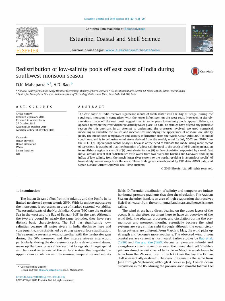
The model is time-integrated for thirty days in prognostic modeas discussed earlier. The model sea surface currents are validatedagainst the corresponding OSCAR currents data of August 2010. Asargued before the current data of August 2002 is similar to that ofAugust 2010 and the validation results are presented in Table 2. Thetable shows some selected statistical parameters for the corre-sponding grid points between the model and OSCAR currents forspeed and direction for 15 August 2002 and 2010. The table alsoshows validation for model SST against Modis/Terra, AVHRR5 SSTfrom http://podaac-w10n.jpl.nasa.gov/w10n/allData/for August2002 and 2010. The SSS data were validated against Argo data. Asnapshot is shown in Fig. 3 for Model and Modis/terra SST forAugust 2002. The AVHRR5 SST is only used to validate SST data for2002 as it is available only up to 2009 and hence not shown here. Itshould be noted that the RMSE is large for SST and SSS as it is validfor the entire analysis region which includes the head bay regionalso. This is due to the large river system discharge at the head bayregion which results in large variations of temperature and salinitythere. As it is evident from the table the model data compares wellwith the observation as far as model produced circulation featuresare concerned. However, the sea surface current direction shows alarge deviation except for the fact that it produced the divergentfeatures of the current around 16.5�N latitudinal belt. The sameOSCAR data will be referred while discussing the results of anom-alous distribution of the low salinity pools to an offshore regionduring August 2010.

(b) Current and salinity distribution: Fig. 4 depict the gradualevolution of surface current (vectors) and salinity (contours) for 7(i.e., 8th August), 14 (i.e., 15th August) and 21 (i.e., 22nd August)days respectively of the model integration for August 2002 andAugust 2010. The coastal circulation from 15�N to 17�N after 7 daysis strong, northeastwards along the coast and the low-salinitydischarge from the two rivers in the coastal zone is retained at

August 2010 0.23 0.05 0.56 0.79Sea Surface SalinityAugust 2002 0.34 0.02 1.1 0.67August 2010 0.42 0.04 1.5 0.65

Fig. 3. (a) Model and (b) Modis/Terra SST (�C) for August 2002.

D.K. Mahapatra, A.D. Rao / Estuarine, Coastal and Shelf Science 184 (2017) 21e29 25

the discharge point which is evident from the 8th August 2002 and2010 of Fig. 4 (Shankar et al., 1996; Durand et al., 2009 andMukherjee et al., 2014). A narrow elongated eddy formed along thecoast around day 15 (the 15th August 2002 and 2010 of Fig. 4) andthe low-salinity pool has migrated away from the coast, signifi-cantly rising the coastal salinity at the discharge location. Further,the insurgence from the north and the curvature of the coastlinehas widened the anticyclonic eddy that led to the shifting of thelow-salinity pool from north to south of 15�N (the 22nd August2002 and 2010 of Fig. 4). The width of the anticyclonic eddy tendsto be more wide when it develops at the lower limb of the curva-ture (15�N) of the coastline than when it forms at the higher one,say, 16.5�N. The salinity at 15.5�N and 16�N is low offshorecompared to the coastal value (Vinayachandran et al., 2015). At15�N however, the coastal and offshore salinity values are nearlysame, with a low-salinity pool prevailing around 81.5�E longitude.It is relevant to recall here that the coastline takes a curvature be-tween 15�N and 16.5�N. As the surface current flows northwardalong the coast, the curvature forces a clock-wise flow and conse-quently deport the low-saline waters offshore. The wind fieldduring the southwest monsoon period is southwesterly and it tendsto beget a northward flow near the coast. Thus, the curvature of thecoastline around 16�N, the southward flowing LSP in the north andthe strong southwesterly winds all culminate in producing an an-ticyclonic tendency in the vicinity. The circulation and the eddy(s)formations are in accordance with the wind stress forcing and theinflux from the north (Benshila et al., 2014 and references therein).

Another important fact which should be noted here is that Fig. 4shows themodel results for two contrastingmonsoon years of 2002which was a week monsoon years having �20% anomaly of LongPeriod Average (LPA) and 2010 which was a normal monsoon yearshaving þ2% anomaly of LPA. In both the cases the net result is samethat is, migration of low salinity pools away from the coast. Thecurrent distribution, the genesis and migration of low salinity poolin both the cases are similar but the salinity distribution andstrength of the low salinity pool vary in both the cases which may

be due to the distribution of southwesterly winds and may also berelated to the dry and wet spell on the pentad scale.

In the absence of more in situ data for surface salinity validation,we made an attempt to validate the model simulated surface cur-rent with near-real time OSCAR ocean surface currents. This isbecause it is believed that the surface circulation has a strongbearing on the distribution of surface waters. In doing so, theemphasis is placed on the surface jet embedded between thesouthward flowing LSP and thewind forced northward current. Theundulations of the jet may be assumed to govern the location of theLSP. In Fig. 4, it may be noticed that the northward flowing surfacejet near the coast tends to get detached at the northern limb, givingway partially to the LSP. As the in situ data shown in Table 1 is forlate July and mid-August, we opted to show the OSCAR current forthat period only, which is depicted in Fig. 5. Thus, Fig. 5 depicts the5-day interval ocean surface current centered on (a) August 8 and(b) August 15 respectively. It may be noticed that the eastwardflowing surface current is squeezed by southward flowing LSP andthe wind driven northward flow from south. It can also be noticedthat the formation of anticyclonic eddy around 15�N is well simu-lated by the model as confirmed by the OSCAR current. The strongoffshore currents of magnitude 50e60 cms-1 between 16 and 17�Nare also endorsed by both model ocean and OSCAR currents whichis mainly responsible for driving the low-salinity pool to anoffshore point (Lucas et al., 2016).

It has been observed that the core of the freshwater plume islocated at a distance of about 100 km from the coast(Vinayachandran and Kurian, 2007) and the insurgence is confinedto north of 17�N. Fig. 6 depicts the Hovmoller diagram for surfacesalinity off 15�N for August 2010 from live access server of IndianNational Centre for Ocean Information Services (http://las.incois.gov.in) which contains ARGO data. The figure shows formation oflow-salinity pool(s) around 10e15 August and there are multiplepools forming and getting advected and dispersed with the strongdivergent current as seen by the OSCAR currents. The low-salinitypools reached as low as 32.8 for these occurrences. From Figs. 5

Fig. 4. Surface current (vectors) and salinity (contours) after 7 days, 14 days and 21 days of model integration for August 2002 (lower panel) and August 2010 (upper panel).

D.K.M

ahapatra,A.D.Rao

/Estuarine,Coastal

andShelf

Science184

(2017)21

e29

26

Fig. 5. 5-day mean ocean surface current (m/s) centered on (a) 8 August 2010 and (b) 15th August 2010 from near real-time ocean surface currents (OSCAR - Ocean Surface CurrentAnalysis-Real-time).

Fig. 6. Hovmoller diagram showing ARGO data with low-salinity pool appearing at an offshore region.[Source: INCOIS LAS server].

D.K. Mahapatra, A.D. Rao / Estuarine, Coastal and Shelf Science 184 (2017) 21e29 27

and 6 it is also evident that the EICC plays a major role in the for-mation, advection and dispersion of these LSPs. The divergentcurrent is strong around 17�N, which may be causing the drifting ofLSPs to offshore points. The OSCAR current shows there is a for-mation and dissipation of eddies near the coast which may beresponsible for shifting the LSPs southward near the coast which isevident in the Hovmoller diagram.

In order to validate the above ARGO data against model resultsof the insurgence of low salinity pool which is confined to north of17�N, the temporal variation of salinity at five locations, viz., 15�N,15.5�N, 16�N, 17�N and 18� N at nearly 100 km from the coast isshown in Fig. 7. It may be seen that at 18�N there is a significant

initial drop of salinity of about 1.8 soon after model integration,indicating the extent of the LSP up to that latitude. There is a steadyrise in salinity at all other locations. It is interesting to note thatalthough the southward flowing surface coastal current is right upto 17�N and beyond, the drop in salinity due to incursion at thecoast is confined to the north of 17�N only. The tongue of relativelyhigh-salinity from about 18.5�N to the offshore of Machilipatnam(16.5�N)may be neutralizing the dilution and hence not reflected inthemodel simulations as well as in-situ hydrographic data. The risein the coastal salinity from 15�N to 16�N is because of the gradualdeporting of the river discharge offshore. The rise at 17�N in salinityoff Kakinada is because of the ensuing offshore transport due to the

Fig. 7. Model simulated temporal evolution of surface salinity near the coast.

D.K. Mahapatra, A.D. Rao / Estuarine, Coastal and Shelf Science 184 (2017) 21e2928

convergence of the coastal currents and the consequent upbringingof the high-saline waters from below. Bathymetry is also contrib-uting anomalous surface salinity fields as the barotropic compo-nent of circulation follows contours of bottom topography withstronger flows being associated with areas over steeper bottomslope.

(c) Influence of coastline curvature: Fig. 8(a and b) depicts thecurrent and salinity after 7 and 14 days of model integration,respectively when the coastline is smoothened out to emphasizethe effect of coastline curvature in driving the low-salinity pooloffshore. The figure clearly indicates due to straight coastline thecurrent structure becomes parallel to coast hampering the forma-tion of anticyclonic eddy and hence, the low-salinity pool getsdispersed as the model integration advances.

Fig. 8. Surface current (vectors) and salinity (contours) after (a) 7 days and (b) 14 days of(Source: Mahapatra, 2012).

4. Summary and conclusion

To understand and comprehend the intriguing fact that low-salinity pool(s) appear offshore compared to the discharge pointof the two perennial rivers, Krishna and Godavari at the east coastof India, numerical modelling has been carried out using realisticwind. The model simulations are validated with in situ CTD andOSCAR data. From the model simulated circulation it is evident thatthe coastal circulation during the southwest monsoon is regulatedby several factors and is complex due to (i) the northward blowingsouthwesterly winds, (ii) the southward influx of low-salinity wa-ters from the north (iii) the freshwater discharge from the tworivers, in the coastal zone, north of 16�N and (iv) the relatively high-saline waters between Gopalpur and Kakinada which hinders thesouthward flowing EICC. It is also assisted favorably by the orien-tation of the coast in the 14�-17�N belt. The curvature of the

model integration with straight coastline.

D.K. Mahapatra, A.D. Rao / Estuarine, Coastal and Shelf Science 184 (2017) 21e29 29

coastline is forcing undulation of the anticyclonic eddy offshore andthe confluence of LSP on either side gradually wears down thetongue of relatively high-salinity between Gopalpur and Kakinada.The study intends to highlight the importance of numericalmodelling to understand coastal circulation and dynamics which isalso dependent on large scale phenomena like monsoon. System-atic numerical modelling approach is required to arrive at somedefinite conclusion. The present study is also useful for policymakers to chalk out plans for identifying potential fishing zonesand their behavior according to seasons.

References

Babu, S.V., Rao, A.D., Mahapatra, D.K., 2008. Pre-monsoon variability of coastalocean processes along the east coast of India. J. Coast. Res. 24, 628e639.

Benshila, R., Durand, F., Masson, S., Bourdall�e-Badie, R., de Boyer, M.C., Papa, F.,Madec, G., 2014. The upper Bay of Bengal salinity structure in a high-resolutionmodel. Ocean. Model. 74, 36e52, 2014.

Blumberg, A.F., Mellor, G.L., 1983. Diagnostic and prognostic numerical circulationstudies of the south Atlantic Bight. J. Geophys. Res. 88, 4579e4592.

Blumberg, A.F., Mellor, G.L., 1987. A description of a three-dimensional coastal oceancirculation model, in Three-Dimensional Coastal Ocean Models. In: Heaps, N.S.(Ed.), Coastal Estuarine Ser, vol. 4. AGU, Washington, D.C, pp. 1e16.

Bowden, K.F., 1983. Physical Oceanography of Coastal Waters. Ellis Horwood Ltd.,Halsted Press, Chichester, UK, p. 302.

Cutler, A.N., Swallow, J.C., 1984. Surface Currents of the Indian Ocean (to 25�S,100�E). Compiled from Historical Data Archived by the Meteorological Office,Bracknel, UK. Report 187. Institute of Oceanographic Sciences, Wormley, UK, pp8 and 36 charts.

Durand, F., Shankar, D., Birol, F., Shenoi, S.S.C., 2009. Spatio-temporal structure ofthe East India coastal current from satellite altimetry. J. Geophys. Res. (C:Oceans) 114 (2), 18. http://dx.doi.org/10.1029/2008JC004807, 2009.

Ezer, T., Mellor, G.L., 1994. Diagnostic and prognostic calculations of the NorthAtlantic circulation and sea level using a sigma coordinate ocean model.J. Geophys. Res. 99 (C7), 14159e14171.

Ezer, T., Thattai, D., Kjerfve, B., 2004. Simulations of the Influence of the WestCaribbean Sea Circulation and Eddies on the Meso-American Barrier Reef Sys-tem. PECS 2004-MERIDA, MEXICO.

Haney, R.L., 1991. On the pressure gradient force over step topography in sigmacoordinate models. J. Phys. Oceanogr. 21, 610e619.

Hastenrath, S., Greischar, L.L., 1989. Climate Atlas of the Indian Ocean, Part-III, UpperOcean Structure, 247 charts. The University of Wisconsin Press.

Holland, W.R., Hirschman, A.D., 1972. A numerical calculation of the circulation inthe North Atlantic Ocean. J. Phys. Oceanogr. 2, 336e354.

Johns, B., Rao, A.D., Rao, G.S., 1992. On the occurrence of upwelling along the eastcoast of India. Estuarine. Coast. Shelf Sci. 35, 75e90.

Liu, X., Wang, J., Cheng, X., Du, Y., 2012. Abnormal upwelling and chlorophyll aconcentration off South Vietnam in summer 2007. J. Geophys. Res. 117 (C07021),10. http://dx.doi.org/10.1029/2012jc008052.

Lucas, A.J., Nash, J.D., Pinkel, R., MacKinnon, J.A., Tandon, A., Mahadevan, A.,Omand, M.M., Freilich, M., Sengupta, D., Ravichandran, M., Le Boyer, A., 2016.Adrift upon a salinity-stratified sea: a view of upper-ocean processes in the Bayof Bengal during the southwest monsoon. Oceanography 29 (2), 134e145.http://dx.doi.org/10.5670/oceanog.2016.46.

Mahapatra, D.K., 2012. Modelling of Coastal Ocean Processes along the IndianCoasts. Ph.D Thesis. IITDelhi, New Delhi, India.

Mukherjee, A., Shankar, D., Fernando, V., et al., 2014. Observed seasonal andintraseasonal variability of the East India Coastal Current on the continentalslope. J. Earth Syst. Sci. 123, 1197. http://dx.doi.org/10.1007/s12040-014-0471-7.

Murty, C.S., Varadachari, V.V.R., 1968. Upwelling along the east coast of India. Bull.Natl. Inst. Sci. India 36, 80e86.

Rao, A.D., Babu, S.V., Prasad, K.V.S.R., Ramana Murty, T.V., Sadhuram, Y.,Mahapatra, D.K., 2010. Investigation of the generation and propagation of lowfrequency internal waves: a case study for the east coast of India, Estuarine.Coast. Shelf Sci. 88, 143e152.

Rao, T.V.N., Rao, B.P., Raju, V.S.R., 1986. Upwelling and sinking along the Visakha-patnam coast. Indian J. Mar. Sci. 15, 84e87.

Rao, T.V.N., Rao, B.P., 1989. Alongshore velocity field off Visakhapatnam, east coastof India during pre-monsoon season. Indian J. Mar. Sci. 18, 46e49.

Shankar, D., McCreary, J.P., Han, W., Shetye, S.R., 1996. Dynamics of the East IndiaCoastal Current - 1. Analytic solutions forced by interior Ekman pumping andlocal alongshore winds. J. Geophys. Res. 101 (C6), 13,975e13,991.

Shetye, S.R., Gouveia, A.D., Shenoi, S.S.C., Michael, G.S., Sundar, D., Almeida, A.M.,Santanam, K., 1991a. The coastal current off western India during the northeastmonsoon. Deep-Sea Reserach 38, 1517e1529.

Shetye, S.R., Shenoi, S.S.C., Gouveia, A.D., Michael, G.S., Sundar, D., Nampoothiri, G.,1991b. Wind-driven coastal upwelling along the western boundary of the Bayof Bengal during the southwest monsoon. Cont. Shelf Res. 11, 1397e1408.

Shetye, S.R., Gouveia, A.D., Shenoi, S.S.C., Sundar, D., Michael, G.S., Nampoothiri, G.,1993. The western boundary current of the seasonal subtropical gyre in the Bayof Bengal. J. Geophys. Res. 98, 945e954.

Shetye, S.R., Gouveia, A.D., Shankar, D., Shenoi, S.S.C., Vinayachandran, P.N.,Sundar, D., Michael, G.S., Nampoothiri, G., 1996. Hydrography and circulation inthe western Bay of Bengal during the northeast monsoon. J. Geophys. Res. 101,14011e14025.

da Silva, A., Young, C., Levitus, S., 1994. 199). Atlas of Surface Marine Data. In: NOAAAtlas NESDIS, vols. 1e5. U.S. Department of Commerce, Washington, pp. 6e10.

Sindhu, B., Suresh, I., Unikrishnan, A.S., Bhatkar, N.V., Neetu, S., Michael, G.S., 2007.Improved bathymetric datasets for the shallow water regions in the IndianOcean. J. Earth Syst. Sci. 116 (3), 261e274.

Vinayachandran, P.N., Jahfer, S., Nanjundiah, R.S., 2015. Impact of river runoff intothe ocean on Indian summer monsoon. Environ. Res. Lett. 10 (5) http://dx.doi.org/10.1088/1748-9326/10/5/054008.

Vinayachandran, P.N., Kurian, J., 2007. Hydrographic observations and modelsimulation of the Bay of Bengal freshwater plume. Deep-Sea Res. I 54, 471e486.