Estimation of the molecular weight distribution in batch polymerization

Estimation of the Molecular Weight Distribution in Batch Polymerization

A filtering technique is proposed for on-line estimation of the temper- ature, monomer conversion, initiator conversion, and the entire molecu- lar weight distribution in a batch methyl methacrylate polymerization reactor. The technique uses a detailed polymerization model combined with on-line measurements of conversion, temperature, and the molecu- lar weight distribution, taken at different discrete time intervals. The polymerization model includes a chain-length-dependent termination rate constant which allows the prediction of the molecular weight distri- bution for common free-radical polymerization conditions. Comparisons between modeling and experimental results show that the polymeriza- tion model gives good predictions of the monomer conversion and the molecular weight distribution in the polymerization system. The perfor- mance of the estimation scheme is tested for cases of strong gel effect conditions leading to a bimodal molecular weight distribution, and poor initial conditions. Finally, off-line experimental data are used to test the algorithm under actual reactor operating conditions.

Mark F. Ellis Department of Chemical Engineering

and Materials Science University of Minnesota Minneapolis, MN 55455

Tad W. Taylor 3M Company

St. Paul, MN 55144

Victor Gonzalez, Klavs F. Jensen Department of Chemical Engineering

and Materials Science University of Minnesota Minneapolis, MN 55455

Introduction

A key polymer property that directly influences the end-use characteristics of the polymer is the molecular weight distribu- tion (MWD). For example, the MWD affects the processing characteristics of the polymer through the melting point and the flow properties of the melted polymer. Also, the molecular weight distribution determines many of the mechanical proper- ties of the processed product, such as its strength and impact resistance. Therefore, there is a strong incentive to be able to control the molecular weight distribution accurately during the course of a polymerization.

In the past, MWD control has been limited to controlling cer- tain average properties of the distribution. Control objectives such as obtaining a particular number-average molecular weight or minimizing the spread in the distribution have typi- cally been used. The control of only average MWD properties was necessary because of limitations in the understanding of polymerization kinetics and on-line polymer property measuring devices. However, control algorithms based on average M W D characteristics (the leading moments of the MWD) are likely to be inaccurate for bimodal and highly skewed distributions. This is unfortunate since bimodal distributions can commonly occur due to phenomena such as the gel effect in free-radical polymer- ization. Balke and Hamielec (1973) and Bogunjoko and Brooks (1 983) have reported experimental observations of bimodal dis-

tributions in methyl methacrylate polymerization. Reichert (1986) has also observed bimodal MWD occurring in isother- mal vinyl acetate polymerization. There may be cases where it is desirable to control a polymerization to achieve a multimodal or skewed distribution, but unless the control scheme can detect the formation of these types of distributions, a reliable control algorithm for this purpose is not possible.

Recent advances in the understanding of the polymerization kinetics for some systems combined with the continuing increases in the computing power of low-cost digital computers, and improved on-line polymer property measuring devices are making the on-line control of the entire M W D feasible. There are still some difficulties associated with the on-line measure- ment of polymer properties which must be solved to control accurately the molecular weight distribution shape. For exam- ple, reliable on-line gel permeation chromatographs (GPC) which provide direct measurements of the MWD have recently become available, but the measurements are plagued by time delays. In addition, certain measurements may be corrupted by noise, and a desired, but unmeasurable polymer property may need to be inferred from other measurements. Kalman filtering is a way to overcome such dificulties and is therefore becoming an area of increasing interest in the polymerization reactor engi- neering literature.

Jo and Bankoff (1976) have applied an extended Kalman fil- ter (EKF) algorithm to a vinyl acetate free radical polymeriza-

AIChE Journal August 1988 Vol. 34, No. 8 1341

tion carried out in a CSTR. Monomer conversion and the weight-average molecular weight of the polymer were estimated by using temperature, refractive index, and impeller torque (correlated with the reaction media solution viscosity) as mea- surements. The estimation was accomplished by means of em- pirical relations which related refractive index with monomer conversion and viscosity with the weight-average molecular weight. The estimator provided good performance in the face of disturbances in the process model and measurements. Hyun et al. (1976) considered the application of the EKF in the continu- ous polymerization of vinyl acetate with low chain branching. In this simulation study, an empirical equation which related the pressure drop of the reacting mixture in a capillary tube to the conversion and molecular weight was used for the on-line detec- tion of process drifts (inhibitor feed rate and residence time vari- ations). The filter was found to be quite robust despite some dif- ficulties in the detection of inhibitor drifts.

Schuler and coworkers (Schuler, 1980; Schuler and Suzhen, 1985; Schuler and Papadopoulou, 1986) developed a decoupled nonlinear estimator based on an EKF for the real-time estima- tion of the chain-length distribution and conversions in a batch polystyrene reactor. The filter used temperature and refractive index measurements. The work by Schuler and Papadopoulou demonstrated the experimental application of the approach. These initial studies did not include the possibility of using on- line GPC measurements and thus errors in the prediction of the chain-length distribution due to disturbances and model errors could not be corrected.

Papadopoulou and Gilles (1 986) and Gilles (1986) later mod- ified this decoupled estimation scheme to include time lagged, discrete gel permeation chromatography measurements in the second portion of the algorithm where the chain-length distribu- tion is estimated. Inclusion of the GPC measurements improved the estimations of the chain-length distribution. The efficiency of the filter was tested for the cases of errors in the initial condi- tions and time varying operating conditions. In this decoupled estimation approach, the chain length distribution (molecular weight distribution) is not fed back to the first part of the esti- mator; therefore it is necessary to assume that the polymer reac- tions rates are independent of chain length. This assumption is not required with the filtering technique presented in this paper.

In this work, we consider the measurement aspect of control- ling the molecular weight distribution shape in a batch methyl methacrylate (MMA) polymerization reactor. We develop a two time scale filter, based on the extended Kalman filter, to estimate monomer and initiator conversions as well as the poly- mer molecular weight distribution from on-line measurements of temperature, monomer conversion, and gel permeation chro- matography. The estimator uses the kinetic model developed by Tulig and Tirrefi (1981) for M M A polymerization which pre- dicts the entire molecular weight distribution, even in the region of strong gel effect conditions.

The estimation scheme, developed to use this detailed poly- merization model in an on-line manner is a departure from pre- vious control-type work. As more powerful computing devices become available for on-line control purposes, the use of com- plex process models in control algorithms is expected to con- tinue. The use of this detailed model in the estimation scheme allows the estimation of the entire M W D rather than only the leading moments of the MWD.

The estimation technique is tested under strong gel effect con- ditions and bimodal distributions. Also, the feasibility of using the filtering algorithm is tested by using off-line experimental measurements of conversion, temperature, and the weight frac- tion of dead polymer to estimate the MWD, monomer conver- sion, initiator conversion, and temperature.

Kinetic Model Development Given the kinetic scheme presented in Table 1, the species

balances incorporating the chain-length dependence of the ter- mination rate constant (assuming no concentration or tempera- ture gradients in the reacting medium) are as follows:

-- 1 d ( R V ) = - k i R M + 2 f k d I V d t

-kdI 1 d ( I V ) --= v d t

rn

- P. k,(n, rn) P,,, (for n > 1) ( 6 ) m-1

--= d(Dn ') k,,s P. S + k,,,,, Pn M + P. 2 k,(n, rn) P,,, (7)

V d t m-1

Table 1. Reactions Known to Occur in the Free-Radical Polymerization of MMA*

k d Initiation 1-2212

k M + R - P ,

k P

ktm

Pn + M - 0, + PI

km P" + s- 0" + PI

Propagation P,, + M - P"+l

Transfer to Monomer

Transfer to Solvent

Termination by Disproportionation

*Termination by combination has been included in the model (Ellis et al., 1987). but was neglected in the work presented here since termination by disproprtiona- tion is the predominant mode of termination in MMA polymerization (Odian, 198 1) and including it caused poorer agreement between predicted and experimen- tal weight- and number-average molecular weight data.

1342 August 1988 Vol. 34, No. 8 AIChE Journal

Here Vdenotes the volume of the reacting mixture, Z is the ini- tiator concentration, R represents the initiated radical concen- tration, and P,, and D, are the polymer concentrations for poly- mer of chain lengths n for live and dead polymer.

To include the effect of the volume change due to polymeriza- tion, the following linear correlation (Tirrell et al., 1987) between volume and monomer conversion is assumed:

Here c - +,,, (p, - pp)/p,, and 4, is the volume fraction of monomer at the start of reaction.

At high monomer conversions an apparent auto-acceleration of the reaction rate occurs, termed the “gel” effect or the Trommsdorff effect. The gel effect model selected was the form used by Coyle et al. (1985), originally developed by Tulig and Tirrell (1981). This model has its origins in the reptation model of polymer diffusion and is given by:

(9)

Here the relation betweenf(n, m, C) and the termination rate constant is:

km( T) is an overall apparent termination rate constant at zero conversion. In this gel effect model the proportionality constant K in Eq. 9 is selected such thatf (1, 1, Ccril) = 1. Before termina- tion becomes strongly diffusion controlled, x, 5 xmrit, the termi- nation rate is assumed to be independent of the chain-lengths of the reacting species and constant.

To determine the critical monomer conversion, xmlit, the fol- lowing relation (Tulig and Tirrell, 1981) has been used:

where xPrit = C,,/M0 ( M o = initial concentration of mono- mer).

At very high conversion levels, for polymerizations with small solvent fractions, the propagation reactions become diffusion controlled, causing a slowing of the rate of polymerization. This phenomenon, the glass propagation effect, was included in the MMA polymerization model (Taylor et al., 1986) by using the correlation of Ross and Laurence (1976) extended for the solu- tion polymerization of MMA, with ethyl acetate as the solvent, by Schmidt and Ray (1981).

To simplify the solution of Eqs. 1 to 7, the continuous variable transformation (Zeman and Amundson, 1963, 1965a,b) was applied in the manner used by Coyle et al. (1985). In order to scale and nondimensionalize the equations, the dimensionless variable formulas presented in Table 2 were used and yielded the following set of nonlinear partial integro-differential equa- tions:

= (1 - dx, dr

dx, dx, d r d7

- = € -

Table 2. Dimensionless Variables and Change of Variable Formulas

Monomer Conversion: x, = (MoVo - MV)/(MoVo) Initiator Conversion: x, - (IoVo - IV)/(IoVo) Reactant Volume: x, - V/Vo Volume Change: e - $,,,(p, - pp)/pm Dead Polymer: x, = DJM, Solvent: x, - S/Mo Living Polymer: xp = Pn/a*, where a* - [ (kd(To)~o)/k,(To)]o’5 Time: 7 - kp( To)a*r Temperature and Rate Constants:

u = TITO

Here C,,, is the critical polymer concentration which corre- sponds to the onset of polymer entanglement, Mn is the number- average molecular weight, and K, and a are constants to be determined from experimental data. The values used for K, and a were determined from data given by Tulig and Tirrell (1981) and found to be a - 0.19 and K, = 2.35 x lo4 where C&t has units of mo1/m3.

The approach proposed by Tulig and Tirrell was developed for bulk polymerization of MMA. For our case involving the solution polymerization of MMA, the value of M,, used for eval- uating C,,, was selected to be the value of M,, when the com- puted conversion x, is equal to 0.20/4,. The validity of using Eq. 9 and this method of determining C,,, for solution polymer- ization of MMA is suggested by polymer solution theory (Tir- rell, 1985). This approximation has been found to produce C, - k,lkD(To), C,,, - k,,Jk,(TJ _ - . . results which are reasonable in MMA solution po1yme;ization. Once C,,, is determined, xMt is obtained from the relation:

a, - [(k,k,l0)/(k:M:)j0.’, all evaluated at T - To

AIChE Journal August 1988 Vol. 34, No. 8 1343

where x,, xI, xu, x,, xp(n) , and xD(n) are dimensionless monomer conversion, initiator conversion, reacting mixture vol- ume, solvent concentration, and live and dead polymer concen- trations for polymer of chain length n. The boundary conditions associated with Eq. 18 are

xp(m) = 0 (19)

and

The second boundary condition above results from applying the pseudosteady-state approximation (PSSA) to initiated radicals Rand live polymer of chain length unity in combination with the long chain hypothesis (i.e., neglecting monomer consumption by initiation relative to that consumed by propagation).

Numerical Solution of the Kinetic Model In order to simplify the solution procedure for the modeling

equations and the evaluation of the integrals appearing in them, the infinite domain of chain lengths involved was replaced with a finite one having a large upper bound, 8. The value of 8 = lo6 was found to be suitable for this system since increasing E fur- ther had a negligible effect on the solution of the modeling equa- tions.

The dead polymer concentration differential equations were solved at discrete chain-length points. The discretization points

were spaced within finite elements a t the zeros of Jacobi orthog- onal polynomials, and the finite elements were equally distrib- uted over the transformed chain length space. Radau quadra- ture weights were used to evaluate the integrals numerically over each finite element. The zeros of the Jacobi polynomials and the Radau quadrature weights were obtained in the manner described by Villadsen and Michelsen (1978).

A transformation given by the relation n = e' was used to con- vert the chain length domain to a logarithmic scale. This was done to have the discretization points spaced more densely in the lower end of the chain length range, where most of the variation in the polymer properties is expected to occur. In addition, one more change of variables, p = PN q, was performed to transform the logarithmic chain length scale to cover the range 0 to 1 to perform numerical integrations using the Radau quadrature weights. These change of variable transformations resulted in the integrals involved being converted to the following forms:

Here Wi are the Radau quadrature weights, xpi represent the dimensionless live polymer concentrations at the chain lengths which correspond to the discretization points (and endpoints of finite elements), ti is the transformed chain length (0 5 q 5 l ) , and N T is the total number of discretization points over the transformed chain length space (the values of N T used are dis- cussed below).

The live polymer concentrations were obtained as the solution to the partial integro-differential equation, Eq. 18. A pseudo- steady-state assumption was invoked to remove the derivative of xp with respect to time in this equation. This approximation has been shown to be valid for MMA polymerization by Tulig (1983) and Coyle et al. (1985). In particular, in the work of Tulig (1983) and Coyle et al. (1985), MMA bulk polymeriza- tion equations with and without the PSSA were solved with only slight differences occurring in the solutions obtained. These dif- ferences were less than those that can be measured experimen- tally.

The resulting equation (after invoking the PSSA) is a second- order ordinary differential equation (ODE). Before the gel effect onset (xm I x,,~,) the integrals wI and w, in Eqs. 18 and 20 can be approximated (Ray, 1972) by [(2fFd(1 - x l ) ) / ( X , F ~ ) ] " ~ ; here f is the efficiency factor for the initiation reac- tion. For this case, the ODE has constant coefficients and has an analytical solution depending on the chain length n, tempera- ture, x,, xu, x,, and xrr which is given by:

1344 August 1988 Vol. 34, No. 8 AICbE Journal

For the case of significant gel effect present (x, > X,~~), the live polymer concentrations cannot be obtained directly using Eq. 23. This is because the approximation made to evaluate inte- grals w , and w2 does not apply after the gel effect onset. The values of xp were obtained by applying the method of successive substitution to Eq. 23 with satisfactory convergence properties.

After applying the above transformations and approxima- tions the resulting set of coupled ODE'S was integrated in time using EPISODE (Hindmarsh and Byrne, 1975).

The number of differential equations to be solved is depen- dent on the number of finite elements and the number ,of discre- tization points distributed within each element. If there are NDZS discretization points within NE finite elements, there will be N T = [ NE( NDZS + I)] dead polymer equations to be inte- grated (the endpoints of each finite element are included except for the last endpoint of the last finite element since this point is taken to be infinity in our formulation and is defined by Eq. 19). Also, there is one differential equation for the monomer mass balance and one more for the initiator mass balance (the solu- tion to the differential equation for the solvent concentration, Eq. 16, was approximated by x, = xa/xD). This therefore gives a total of [NE(NDZS + 1) + 21 modeling equations to be inte- grated for a particular simulation.

Appropriate choices for NE and NDIS have been determined to be NE = 15 and NDZS = 2 (Ellis, 1989), giving 47 differen- tial equations to be solved. This selection provided adequate resolution of the polymer concentrations to perform the numer- ical integrations required in solving the modeling equations. Increasing NDIS or NE had no appreciable effect on the pre- dicted conversions or MWD, but escalated the computation time. On the other hand, ten finite elements and two interior dis- cretization points were not sufficient to resolve the MWD; the average molecular weight properties deviated from those calcu- lated with more finite elements. For all simulation and estima- tion results presented in this paper, two discretization points dis- tributed within 15 finite elements were used.

As an alternate to the procedure described above for solving the modeling equations, orthogonal collocation on finite ele- ments was also used. The first and second order derivatives of xp with respect to n in Eq. 18 were approximated using the approaches outlined by Finlayson (1980) and Villadsen and Michelsen (1978). The derivative of x, with respect to 7 was neglected by using the pseudosteady-state approximation de- scribed above. The resulting set of nonlinear algebraic equations was solved using the Newton-Raphson method. The remainder of the solution procedure was the same as already described. It was found that the orthogonal collocation procedure was less efficient and less accurate than the method described above, and therefore abandoned.

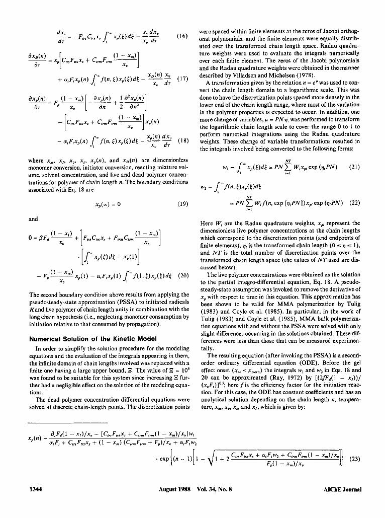
Experimental System Figure 1 depicts the schematic diagram for the methyl meth-

acrylate polymerization system. As illustrated in the figure, some portions of this diagram are still under development, but the entire system has been shown to illustrate the assumed con- figuration for the estimation results presented below. A 1.5 x lo-' m3 jacketed glass reactor was used for batch solution polymerizations. The solvent was ethyl acetate (anhydrous, GR grade from EM Science) and the initiator was azobisisobutyro-

AIChE Journal August 1988

cold wsta

EMCON - m CONTROL COMPUTER

Figure 1. MMA batch reactor system (the portion en- closed by the box is under development).

nitrile (AIBN), supplied by DuPont. The methyl methacrylate, supplied by Rohm and Haas, contained hydroquinone inhibitor to prevent polymerization during storage. The inhibitor was removed by passing the MMA through an amberlyst ion exchange resin and then further purified by vacuum distillation (298-308 K). Polymerizations were performed after purging the monomer and solvent of oxygen (a reaction inhibitor) by bubbling nitrogen through them for approximately a half hour. The nitrogen purge was also continued during the polymeriza- tions. The reaction media was stirred using a paddle stirrer (0.09 m in diameter and 0.03 m in height) at 250 RPM. All GPC mea- surement results presented were obtained in an off-line manner using a Waters chromatograph (model 150-C ALC/GPC) with Polymer Labs columns (lo3, lo4, and lo5 A). Off-line monomer conversion measurements were obtained by using gravimetric methods.

Three recirculation loops are associated with the reaction sys- tem. One loop is used for computer-controlled heating and cool- ing of the reaction media. The second loop, which is under devel- opment, pumps the reaction fluid through a Mettler-Paar on- line densitometer. The densitometer will be used to determine the monomer conversion during polymerization. Since the den- sity of polymer in MMA polymerization is greater than that of the monomer, a mass balance relation (Ponnuswamy, 1984; Ponnuswamy et al., 1986) has been used with good success for inferring monomer conversion from density measurements (El- lis et al., 1988). Schork and Ray (1981) and Ponnuswamy et al. (1986) have reported accurate, reproducible results using the same type of densitometer for monomer conversion determina- tion. The third loop, also under development, is designed for pumping the batch reactor's contents through an Applied Auto- mation on-line GPC for periodic on-line MWD measurements.

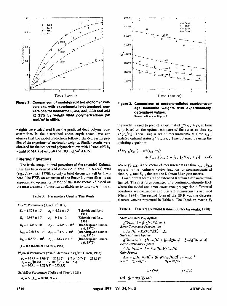
Model Validation Figure 2 presents a comparison between experimental

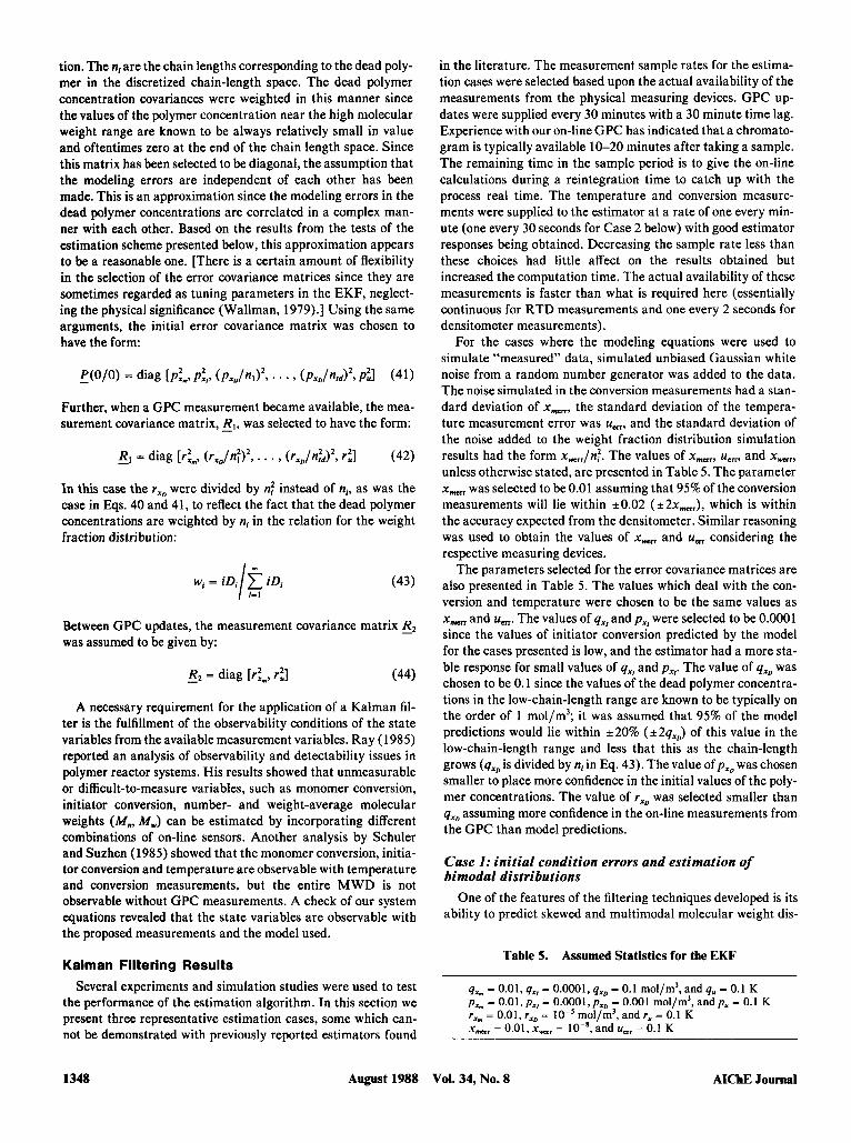
monomer conversion values and model predictions v. time for a 25% by weight MMA polymerization (50 mol/m3 AIBN) car- ried out at different reaction temperatures. The agreement is quite good considering that no parameters have been fitted (model parameters used in the simulations appear in Table 3). Figure 3 shows the corresponding experimental and predicted number-average molecular weights for the polymerization re- sults in Figure 2. The simulated number-average molecular

Vol. 34, No. 8 1345

o - 323K + 0 - - 338K 3333 o - 3433 /A

0.

Time (hours)

Figure 2. Comparison of model-predicted monomer con- versions with experimentally-determined con- versions for isothermal (323,333,338 and 343 K) 25% by weight MMA polymerizations (50 mol/m3 In AIBN).

weights were calculated from the predicted dead polymer con- centrations in the discretized chain-length space. We can observe that the model predictions followed the decreasing pro- files of the experimental molecular weights. Similar results were obtained for the isothermal polymerizations with 10 and 40% by weight MMA and with 50 and 100 mol/m' AIBN.

Filtering Equations The basic computational procedure of the extended Kalman

filter has been derived and discussed in detail in several texts (e.g., Jazwinski, 1970), so only a brief discussion will be given here. The EKF, an extension of the linear Kalman filter, is an approximate optimal estimator of the state vector x* based on the measurement information available up to time T ~ . At time T~

Table 3. Parameters Used in This Work

Kinetic Parameters (J, mol, m', K, s) Ep - 1.824 x lo4

El = 2.937 x 10'

Ed - 1.228 x Id

E,,,,, ... 7.513 x lo4

A, - 4.92 x 10'

A, - 9.8 x lo'

Ad - 1.2525 x lOI4

A,,,,, - 7.177 x lo6

(Schmidt and Ray,

(Schmidt and Ray,

(Brandrup and Immer-

(Brandrupand Immer-

1981)

1981)

gut, 1975)

gut, 19%) Elm - 6.570 x lo4 A,,, - 4.673 x lo5 (Brandrup and Immer-

gut, 1975) f- 0.5 (Schmidt and Ray, 1981)

Physical Parameters (Tin K , densities in kg/m'; Clinch, 1983)

P,,, - 965.4 - 1.09(T - 273.15) - 9.7 x IO-'(T - 273.15)2 pp - pm/[0.754 - 9 x lOW4(T - 343.15)] pz - 925.0 - 1.237(T - 273.15)

Gel Efect Parameters (Tulig and Tirrell, 198 1)

N, - 5 0 . f ~ . - 0.001,B - 2

i 0 - 323K + - 333K 0 - 338K - 343K

70000

10000 -

Time (hours)

Figure 3. Comparison of model-predicted number-aver- age molecular weights with experimentally- determined values. Same conditions as Figure 2.

the model is used to predict an estimated ~ * ( T ~ + ~ / T ~ ) , at time T ~ + ~ , based on the optimal estimate of the states at time T ~ ,

x * ( T ~ / T ~ ) . Then using a set of measurements at time T ~ + ~ ,

updated optimal states x* ( T ~ + ~ / T ~ + ~ ) are obtained by using the updating algorithm:

- X* (~t+i/~t+i) = X* (7t+i/~d + Kk+11Y(Tk+I) - !,+I [ ~ * ( ~ t + 1 / . , ) 1 1 (24)

where Z ( T ~ + ~ ) is the vector of measurements at time T ~ + ~ , 4+, represents the nonlinear vector function for measurements at time T ~ + ~ , and &+, denotes the Kalman filter gain matrix.

Two different forms of the extended Kalman filter were inves- tigated. The first form consisted of a continuous-discrete EKF where the model and error covariance propagation differential equations are continuous and discrete measurements are used (Gelb, 1974). The second form of the EKF was the discrete- discrete version presented in Table 4. The Jacobian matrix Ek Table 4. Discrete Extended Kalman Filter (Jazwinski, 1970)

1346 August 1988 VoI. 34, No. 8 AIChE Journal

required for these two EKF schemes was evaluated as described by Ellis (1989). To use the discrete-discrete EKF the continuous model equations, Eqs. 13 to 17, were discretized by integrating the model equations and approximating the nonlinearities of the system as constant over the time interval Ark (sampling time). That is, the portions of Eqs. 13 to 17 appearing as a,, a2, and a3 in Eqs. 28 to 30 below were assumed constant over a sampling interval, allowing the analytical integration of Eqs. 13 to 17. This procedure yielded the following prediction equations:

where

conversion measurements and the slow time scale is used to accommodate MWD measurements. When a GPC measure- ment is available, the system and filter equations are reinitial- ized to the original GPC sample time and then reintegrated to the process real time. For the reintegraton, the old values of measured temperature and conversion (stored in the estimation algorithm) are used as the measurements. Thus the reintegra- tion provides improved estimates of temperature and conver- sions using the most recent GPC update, and the molecular weight distribution is predicted until the next GPC update becomes available.

When a GPC measurement is incorporated in the estimator, the temperature, conversion, and GPC measurements are de- scribed by:

A F d (29)

Here Xm(Tk+l/Tk)r x , ( T ~ + I / T ~ ) and z ~ ( T ~ + , / T ~ ) are the predicted estimates of monomer conversion, initiator conversion, and dead polymer concentrations evaluated at time T ~ + , given the optimal state estimates at time T k . The temperature was estimated as a measurable model parameter. Therefore, the set of continuous prediction equations were augmented with ti = 0 and the dis- crete prediction equations, Eqs. 25 to 30, were augmented with the equation u ( T ~ + ~ / 7 k ) = u ( T k / r k ) .

The continuous-discrete estimator gave a good response, but

Here y , is the temperature measurement corrupted by the error T~ and y 2 is the conversion measurement with measurement error v 2 . wf = [wJ,, . . . , wJNTIT where w/., are the dead polymer weight frzctions at the chain lengths corresponding to the points in the discretized chain length space, r d is the time delay involved in the GPC characterization, and ?,is the error in the GPC measurement. ~ $ 7 ~ ) = [v1v2y/T] is a white measurement noise characterized by:

In between GPC updates, the measurement equations are given by Eqs. 32 and 33. For this case the measurement statistics and the measurement error covariance matrix, R2, are described by:

was computationally slow for on-line estimations (taking on the order of days to simulate a four-hour estimation using an Apollo DN3000 Workstation). The discrete-discrete version gave es- sentially the same results as the continuous-discrete form while

and

(37) E{[vl(~k)v2(Tk)lT1 = 2 keeping the computation time within bounds for use in a real- time, on-line state estimation. That is, a simulated four-hour Gaussian white noise with statistics given by:

estimation required less than two hours using an Apollo DN3000. For all estimation studies presented below, the dis- Crete-discrete EKF was used.

The states to be estimated are the monomer conversion x,, the initiator conversion x,, the dead polymer concentrations at

are used to represent model uncertainties in a s . 25 to 30. Simi- larly, initial statistics of the state variables are given by:

chain lengths which correspond to the discretization points in the dead polymer discretization x,, and the reaction tempera- ture. The vector of states has the following form:

E ( : ( o ) ~ ~ ( o ) l = p ( O / O ) and E{x(O)l = x0 (39)

The measurement and modeling errors were assumed to be uncorrelated with time. The modeling error covariance matrix was chosen to have the form: (31) = [xmx,&4]

where 50 = 1XD.l xD.2 . . . XD,NTI T* Measurements of Drocess states are available onlv at discrete

times. Since GPC measurements are generally available at a slower rate than the conversion and temperature measurements, and they are time delayed, the standard Kalman filter approach was modified to operate on two time scales in the following man- ner. The first time scale is for the relatively fast temperature and

Here qx,, qx,, qy are the standard deviations assumed for the modeling errors of monomer conversion, initiator conversion, and temperature, respectively. qx,,/ni are the assumed standard deviations for the modeling errors of dead polymer concentra-

AIChE Journal August 1988 Vol. 34, No. 8 1347

tion. The n, are the chain lengths corresponding to the dead poly- mer in the discretized chain-length space. The dead polymer concentration covariances were weighted in this manner since the values of the polymer concentration near the high molecular weight range are known to be always relatively small in value and oftentimes zero a t the end of the chain length space. Since this matrix has been selected to be diagonal, the assumption that the modeling errors are independent of each other has been made. This is an approximation since the modeling errors in the dead polymer concentrations are correlated in a complex man- ner with each other. Based on the results from the tests of the estimation scheme presented below, this approximation appears to be a reasonable one. [There is a certain amount of flexibility in the selection of the error covariance matrices since they are sometimes regarded as tuning parameters in the EKF, neglect- ing the physical significance (Wallman, 1979).] Using the same arguments, the initial error covariance matrix was chosen to have the form:

Further, when a GPC measurement became available, the mea- surement covariance matrix, El, was selected to have the form:

In this case the r,, were divided by nf instead of n,, as was the case in Eqs. 40 and 41, to reflect the fact that the dead polymer concentrations are weighted by n, in the relation for the weight fraction distribution:

wi = iD, iD, / (43)

Between GPC updates, the measurement covariance matrix E2 was assumed to be given by:

- R2 = diag [r:,, r t ] (44)

A necessary requirement for the application of a Kalman fil- ter is the fulfillment of the observability conditions of the state variables from the available measurement variables. Ray (1985) reported an analysis of observability and detectability issues in polymer reactor systems. His results showed that unmeasurable or difficult-to-measure variables, such as monomer conversion, initiator conversion, number- and weight-average molecular weights (M,,, M,,,) can be estimated by incorporating different combinations of on-line sensors. Another analysis by Schuler and Suzhen (1985) showed that the monomer conversion, initia- tor conversion and temperature are observable with temperature and conversion measurements, but the entire M W D is not observable without GPC measurements. A check of our system equations revealed that the state variables are observable with the proposed measurements and the model used.

Kalman Filtering Results Several experiments and simulation studies were used to test

the performance of the estimation algorithm. In this section we present three representative estimation cases, some which can- not be demonstrated with previously reported estimators found

in the literature. The measurement sample rates for the estima- tion cases were selected based upon the actual availability of the measurements from the physical measuring devices. GPC up- dates were supplied every 30 minutes with a 30 minute time lag. Experience with our on-line GPC has indicated that a chromato- gram is typically available 10-20 minutes after taking a sample. The remaining time in the sample period is to give the on-line calculations during a reintegration time to catch up with the process real time. The temperature and conversion measure- ments were supplied to the estimator a t a rate of one every min- ute (one every 30 seconds for Case 2 below) with good estimator responses being obtained. Decreasing the sample rate less than these choices had little affect on the results obtained but increased the computation time. The actual availability of these measurements is faster than what is required here (essentially continuous for RTD measurements and one every 2 seconds for densitometer measurements).

For the cases where the modeling equations were used to simulate “measured” data, simulated unbiased Gaussian white noise from a random number generator was added to the data. The noise simulated in the conversion measurements had a stan- dard deviation of x,,, the standard deviation of the tempera- ture measurement error was uc,, and the standard deviation of the noise added to the weight fraction distribution simulation results had the form x,, /nf. The values of x,,,,,, uerr, and x,,, unless otherwise stated, are presented in Table 5. The parameter x,, was selected to be 0.01 assuming that 95% of the conversion measurements will lie within k0.02 (c~x,,,), which is within the accuracy expected from the densitometer. Similar reasoning was used to obtain the values of x,, and u,, considering the respective measuring devices.

The parameters selected for the error covariance matrices are also presented in Table 5. The values which deal with the con- version and temperature were chosen to be the same values as x,, and u,,,. The values of q,, and pxr were selected to be 0.0001 since the values of initiator conversion predicted by the model for the cases presented is low, and the estimator had a more sta- ble response for small values of qx, and pxl. The value of qxo was chosen to be 0.1 since the values of the dead polymer concentra- tions in the low-chain-length range are known to be typically on the order of 1 mol/m3; it was assumed that 95% of the model predictions would lie within ~ 2 0 % (~2q,,) of this value in the low-chain-length range and less that this as the chain-length grows (qx, is divided by n, in Eq. 43). The value ofp,, was chosen smaller to place more confidence in the initial values of the poly- mer concentrations. The value of rxD was selected smaller than qxo assuming more confidence in the on-line measurements from the GPC than model predictions.

Case I : initial condition errors and estimation of bimodal distributions

One of the features of the filtering techniques developed is its ability to predict skewed and multimodal molecular weight dis-

Table 5. Assumed Statistics for the EKF

qx, = 0.01, qxl = 0.0001, qxo = 0.1 mol/m’, and q. = 0.1 K p,-0.01,p,,-0.0001,p,,,=0.001 mol/m3,andp,=0.1 K rxm = 0.01, rxD - lo-’ mol/m’, and r, = 0.1 K x,, - 0.01, x, = lo-*, and u., = 0.1 K

1348 August 1988 Vol. 34, No. 8 AIChE Journal

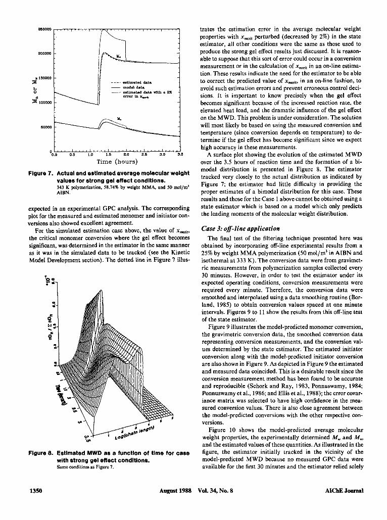
tributions. Figures 4 to 6 show estimation results were a small amount of low-molecular-weight polymer was initially present in the reactor but unknown to the estimator. This possibility could occur if the reactor was improperly cleaned after the pre- vious polymerization. The low-molecular-weight polymer ini- tially present in the reactor was from a simulated three-minute polymerization with operating conditions consisting of MMA with a weight fraction of 0.019, isothermal a t 363 K and 50 mol/ m3 in AIBN. The conditions for the 12 hour polymerization were 323 K isothermal, AIBN initially 50 mol/m3, and MMA with an initial weight fraction of 0.4172.

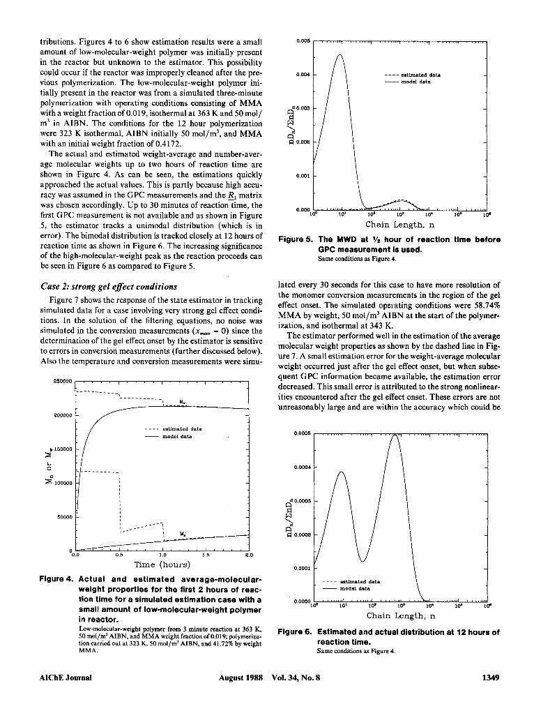
The actual and estimated weight-average and number-aver- age molecular weights up to two hours of reaction time are shown in Figure 4. As can be seen, the estimations quickly approached the actual values. This is partly because high accu- racy was assumed in the GPC measurements and the El matrix was chosen accordingly. Up to 30 minutes of reaction time, the first GPC measurement is not available and as shown in Figure 5, the estimator tracks a unimodal distribution (which is in error). The bimodal distribution is tracked closely at 12 hours of reaction time as shown in Figure 6. The increasing significance of the high-molecular-weight peak as the reaction proceeds can be seen in Figure 6 as compared to Figure 5.

Case 2: strong gel eflect conditions Figure 7 shows the response of the state estimator in tracking

simulated data for a case involving very strong gel effect condi- tions. In the solution of the filtering equations, no noise was simulated in the conversion measurements (x,,, = 0) since the determination of the gel effect onset by the estimator is sensitive to errors in conversion measurements (further discussed below). Also the temperature and conversion measurements were simu-

200000

# 150000 s

50000 [ II ' ~ - - - - - - i

I _ - -

I &-

0.5 1.0 1.5 2.0

Time (hours)

Figure 4. Actual and estimated average-molecular- weight properties for the first 2 hours of reac- tion time for a simulated estimation case with a small amount of low-molecular-weight polymer in reactor. Low-molecular-weight polymer from 3 minute reaction at 363 K, 50 mol/m' AIBN, and MMA weight fraction of 0.019; polymeriza- tion carried out at 323 K, 50 mol/m' AIBN, and 41.72% by weight MMA.

AIChE Journal August 1988

O.Ool 5 estimated data _ _ _ _

- model data 0.004

0.003

d 3 d 0.002

0.001

0.000 1 00 10' 1 0' 1 0' 1 0' 10'

Chain Length, n

Figure5. The MWD at hour of reaction time before GPC measurement is used. Same conditions as Figure 4.

lated every 30 seconds for this case to have more resolution of the monomer conversion measurements in the region of the gel effect onset. The simulated operating conditions were 58.74% MMA by weight, 50 mol/m' AIBN at the start of the polymer- ization, and isothermal a t 343 K.

The estimator performed well in the estimation of the average molecular weight properties as shown by the dashed line in Fig- ure 7. A small estimation error for the weight-average molecular weight occurred just after the gel effect onset, but when subse- quent GPC information became available, the estimation error decreased. This small error is attributed to the strong nonlinear- ities encountered after the gel effect onset. These errors are not unreasonably large and are within the accuracy which could be

0.0001

0.0004

a" 0.0°03 d W

-2 d 0.0002

0.0001

0.0000

_ _ - _ estlmatsd data - model data

I , ,,,,,,,I , , , , 1 1 1 1 1 I I , , (I , 1 1 1 1 1 1 1 1 I , ' Y

10' 1 0' 10' 104 10'

Chain Length, n

Flgure 6. Estimated and actual distribution at 12 hours of reaction time. Same conditions as Figure 4.

Vol. 34, No. 8 1349

trates the estimation error in the average molecular weight properties with xmrit perturbed (decreased by 2%) in the state estimator, all other conditions were the same as those used to produce the strong gel effect results just discussed. It is reason- able to suppose that this sort of error could occur in a conversion measurement or in the calculation of xmriI in an on-line estima- tion. These results indicate the need for the estimator to be able to correct the predicted value of xmit, in an on-line fashion, to avoid such estimation errors and prevent erroneous control deci-

becomes significant because of the increased reaction rate, the elevated heat load, and the dramatic influence of the gel effect on the MWD. This problem is under consideration. The solution will most likely be based on using the measured conversion and temperature (since conversion depends on temperature) to de- termine if the gel effect has become significant since we expect

200000

estimated data

error in q.,,,,

2 lsOOOO

emtimated data with a 2% h 0

0 sions. It is important to know precisely when the gel effect z 100000

60000

1, , , I I , , , , I , , , , I , , , , I , , , , I , , I , I , , , , j high accuracy in these measurements. '0.0 0.6 1.0 1.5 2.0 2.5 3.0 3.6 A surface plot showing the evolution of the estimated MWD

Time (hours) over the 3.5 hours of reaction time and the formation of a bi- modal distribution is presented in Figure 8. The estimator tracked very closely to the actual distribution as indicated by Figure 7; the estimator had little difficulty in providing the proper estimates of a bimodal distribution for this case. These

Figure 7. Actual and estimated average molecular weight values for strong gel effect conditions. 343 58.,4x by weight MMA, and mol,ml AIBN.

expected in an experimental GPC analysis. The corresponding plot for the measured and estimated monomer and initiator con- versions also showed excellent agreement.

For the simulated estimation case above, the value of xdtr the critical monomer conversion where the gel effect becomes significant, was determined in the estimator in the same manner as it was in the simulated data to be tracked (see the Kinetic Model Development section). The dotted line in Figure I illus-

Figure 8. Estimated MWD as a function of time for case with strong gel effect conditions. Same conditions as Figure 7.

results and those for the Case 1 above cannot be obtained using a state estimator which is based on a model which only predicts the leading moments of the molecular weight distribution.

Case 3: 08-line application The final test of the filtering technique presented here was

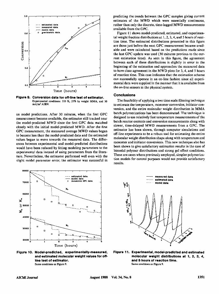
obtained by incorporating off-line experimental results from a 25% by weight MMA polymerization (50 mol/m' in AIBN and isothermal at 333 K). The conversion data were from gravimet- ric measurements from polymerization samples collected every 30 minutes. However, in order to test the estimator under its expected operating conditions, conversion measurements were required every minute. Therefore, the conversion data were smoothed and interpolated using a data smoothing routine (Bor- land, 1985) to obtain conversion values spaced at one minute intervals. Figures 9 to 1 1 show the results from this off-line test of the state estimator.

Figure 9 illustrates the model-predicted monomer conversion, the gravimetric conversion data, the smoothed conversion data representing conversion measurements, and the conversion val- ues determined by the state estimator. The estimated initiator conversion along with the model-predicted initiator conversion are also shown in Figure 9. As depicted in Figure 9 the estimated and measured data coincided. This is a desirable result since the conversion measurement method has been found to be accurate and reproducible (Schork and Ray, 1983, Ponnuswamy, 1984; Ponnuswamy et al., 1986; and Ellis et al., 1988); the error covar- iance matrix was selected to have high confidence in the mea- sured conversion values. There is also close agreement between the model-predicted conversions with the other respective con- versions.

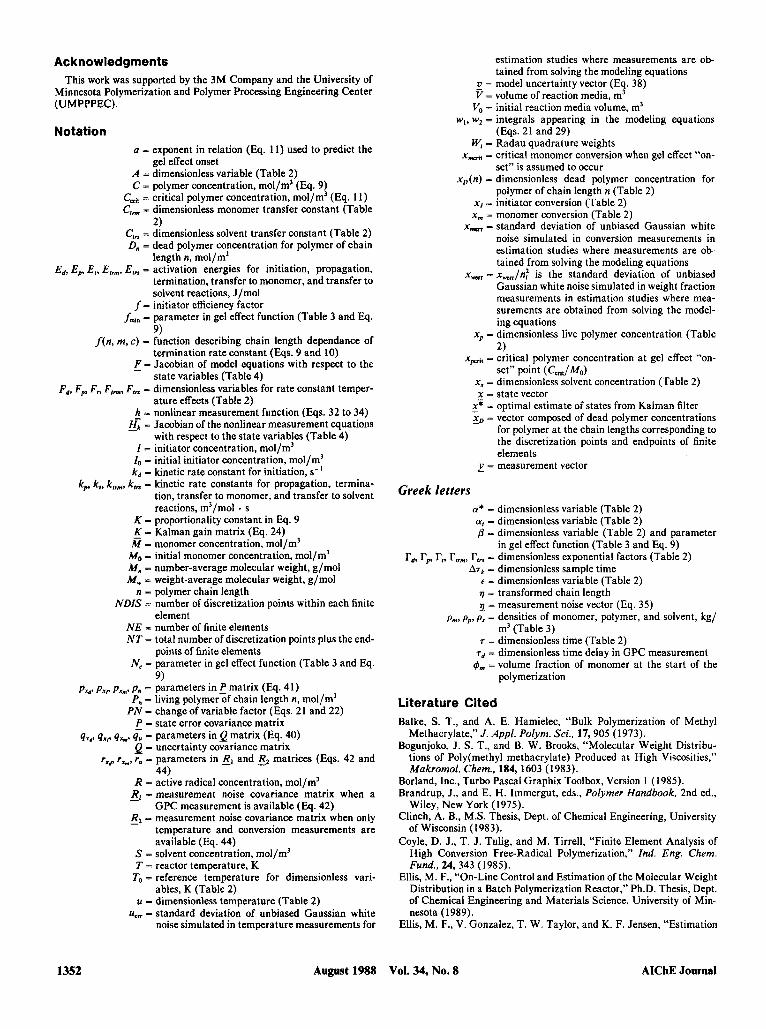
Figure 10 shows the model-predicted average molecular weight properties, the experimentally determined M , and M,, and the estimated values of these quantities. As illustrated in the figure, the estimator initially tracked in the vicinity of the model-predicted MWD because no measured GPC data were available for the first 30 minutes and the estimator relied solely

1350 August 1988 Vol. 34, No. 8 AICbE Journai

0.8

- - - eatimated data measured data

o gradmetric data 0.8

E

E

.A vl

0.4 * V

0.2

0.0 1 2 3 4 6

Time (hours)

Figure 9. Conversion data for off-line test of estimator.

mo1/m3 AIBN. Experimental conditions: 333 K, 25% by weight MMA, and 50

on model predictions. After 30 minutes, when the first GPC measurement became available, the estimator still tracked near the model-predicted MWD since the first GPC data matched closely with the initial model-predicted MWD. After the first GPC measurement, the measured average MWD values began to become less than the model-predicted data and the estimated values began to move towards the measured data. The differ- ences between experimental and model-predicted distributions would have been reduced by fitting modeling parameters to the experimental data instead of using parameters from the litera- ture. Nevertheless, the estimator performed well even with the slight model parameter error; the estimator was successful in

BOO00

70000

80000

2 60000

9 40000

30000

20000

, 0

1

Time (hours)

Figure 10. Model-predicted, experimentally-measured, and estimated molecular weight values for off- line test of estimator. Same conditions as Figure 9.

predicting the trends between the GPC samples giving current estimates of the MWD which were essentially continuous, rather than only the discrete, time-lagged MWD measurements available from the GPC.

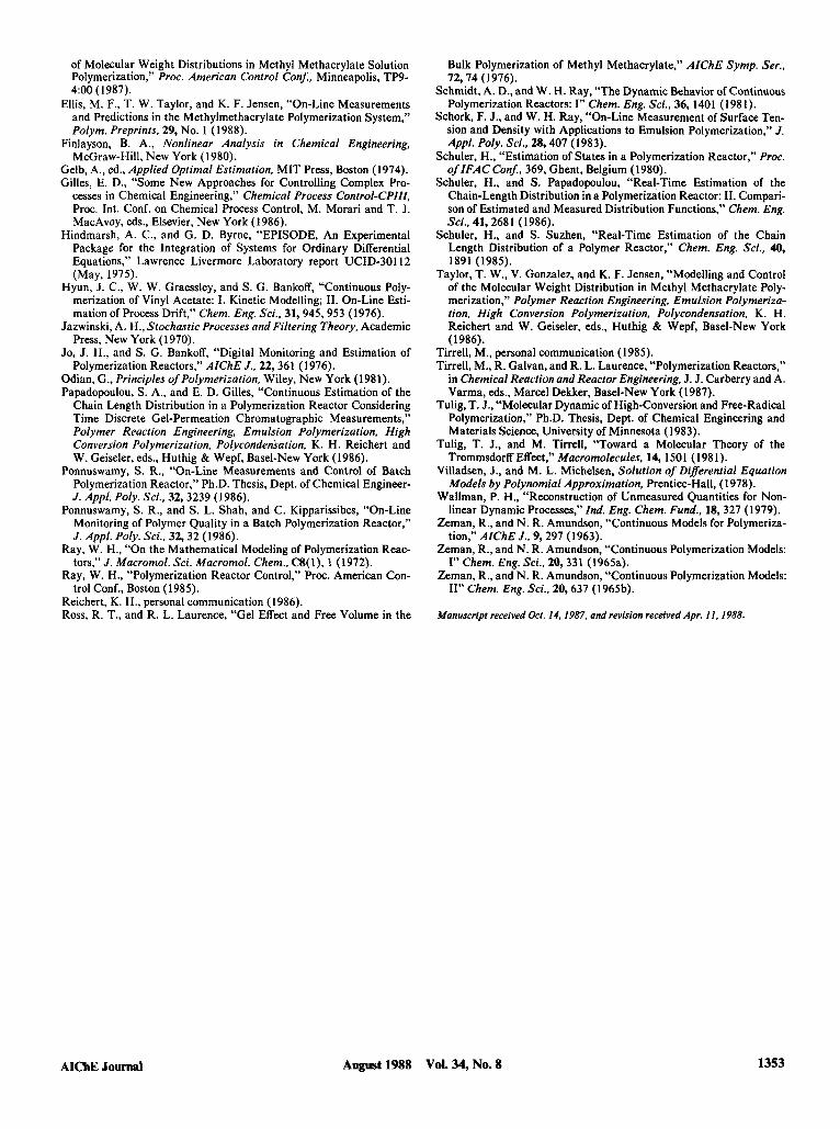
Figure 1 1 shows model-predicted, estimated, and experimen- tal weight fraction distributions at 1,2,3,4, and 5 hours of reac- tion time. The estimated distributions presented in this figure are those just before the next GPC measurement became avail- able and were calculated based on the predictions made since the last GPC update was used (30 minutes previous to the cur- rent estimation time). As seen in this figure, the agreement between each of these distributions is slightly in error in the beginning of the estimation and approaches the measured data to have close agreement in the MWD plots for 3,4, and 5 hours of reaction time. This case indicates that the estimation scheme can successfully operate in an on-line fashion since all experi- mental data were supplied in the manner that it is available from the on-line sensors in the physical system.

Conclusions The feasibility of applying a two time scale filtering technique

to estimate the temperature, monomer conversion, initiator con- version, and the entire molecular weight distribution in MMA batch polymerizations has been demonstrated. The technique is designed to use relatively fast temperature measurements of the batch reactor contents and conversion measurements along with slower, time-delayed MWD measurements from a GPC. The estimator has been shown, through computer simulations and off-line experiments to be a robust tool for estimating the entire molecular weight distribution shape along with temperature and monomer and initiator conversions. This new technique also has been shown to give satisfactory estimation results in the case of bimodal polymer distributions and strong gel effect conditions. These are cases where previously employed, simpler polymeriza- tion models for control purposes would not provide satisfactory results.

maarured data ertlmatad data modal data

- . . .. .. . . .

6

Figure 1 1. Experimental, model-predicted and estimated molecular weight distributions at 1, 2, 3, 4, and 5 hours of reaction time. Same conditions as Figure 9.

AIChE Journal August 1988 Vol. 34, No. 8 1351

Acknowledgments This work was supported by the 3M Company and the University of

Minnesota Polymerization and Polymer Processing Engineering Center (UMPPPEC).

Notation a - exponent in relation (Eq. 11) used to predict the

A = dimensionless variable (Table 2) C = polymer concentration, mol/m3 (Eq. 9)

gel effect onset

Cdt = critical polymer concentration, mol/m3 (Eq. 11) C,, = dimensionless monomer transfer constant (Table

2) C,, = dimensionless solvent transfer constant (Table 2) Dm = dead polymer concentration for polymer of chain

length n, mol/m3 Ed, E,,, E,, Elm, El,* = activation energies for initiation, propagation,

termination, transfer to monomer, and transfer to solvent reactions, J/mol

f = initiator efficiency factor fmin = parameter in gel effect function (Table 3 and Eq.

f ( n , m, c) = function describing chain length dependance of

= Jacobian of model equations with respect to the

Fdr F,,, Fl, F,,, F,,, - dimensionless variables for rate constant temper-

9)

termination rate constant (Eqs. 9 and 10)

state variables (Table 4)

ature effects (Table 2) h = nonlinear measurement function (Eqs. 32 to 34)

gy - Jacobian of the nonlinear measurement equations with respect to the state variables (Table 4)

I = initiator concentration, moI/m3 z0 = initial initiator concentration, moI/m3 kd = kinetic rate constant for initiation, s-’

k,,, k,, k,, k,, - kinetic rate constants for propagation, termina- tion, transfer to monomer, and transfer to solvent reactions, m3/mo1 . s

K - proportionality constant in Eq. 9 K = Kalman gain matrix (Eq. 24) Zi = monomer concentration, mo1/m3

M~ - initial monomer concentration, moI/m3 M. = number-average molecular weight, g/mol M, = weight-average molecular weight, g/mol

n - polymer chain length NDIS = number of discretization points within each finite

element N E = number of finite elements N T = total number of discretization points plus the end-

N, = parameter in gel effect function (Table 3 and Eq. points of finite elements

9) pxd, p,,, pIm, p. = parameters in f matrix (Eq. 41)

P. = living polymer of chain length n, mol/m3 PN = change of variable factor (Eqs. 21 and 22) P - state error covariance matrix

Q = uncertainty covariance matrix

R = active radical concentration, mol/m3

- qx. qlp qs, q. - parameters in Q matrix (Eq. 40)

rx8 r.,, ru - parameters in R, and RZ matrices (Eqs. 42 and 44)

El - measurement noise covariance matrix when a GPC measurement is available (Eq. 42)

- R2 - measurement noise covariance matrix when only temperature and conversion measurements are available (Eq. 44)

S = solvent concentration, moI/m3 T = reactor temperature, K

To = reference temperature for dimensionless vari- ables, K (Table 2)

u = dimensionless temperature (Table 2) u, - standard deviation of unbiased Gaussian white

noise simulated in temperature measurements for

estimation studies where measurements are ob- tained from solving the modeling equations

u = model uncertainty vector (Eq. 38) v = volume of reaction media, m3 Vo = initial reaction media volume, m3

w,, w, = integrals appearing in the modeling equations (Eqs. 21 and 29)

W, = Radau quadrature weights x-, - critical monomer conversion when gel effect “on-

x,(n) = dimensionless dead polymer concentration for set” is assumed to occur

polymer of chain length n (Table 2) x, - initiator conversion (Table 2) x, - monomer conversion (Table 2)

x,, = standard deviation of unbiased Gaussian white noise simulated in conversion measurements in estimation studies where measurements are ob- tained from solving the modeling equations

x, = x,/nf is the standard deviation of unbiased Gaussian white noise simulated in weight fraction measurements in estimation studies where mea- surements are obtained from solving the model- ing equations

x,, = dimensionless live polymer concentration (Table 2)

xpfit = critical polymer concentration at gel effect “on- set” point (Ccrit/Mo)

x, = dimensionless solvent concentration (Table 2) x = state vector - x* - optimal estimate of states from Kalman filter xD = vector composed of dead polymer concentrations

for polymer at the chain lengths corresponding to the discretization points and endpoints of finite elements

-

)! = measurement vector

Greek letters a* = dimensionless variable (Table 2) a, = dimensionless variable (Table 2) j3 = dimensionless variable (Table 2) and parameter

in gel effect function (Table 3 and Eq. 9) r,, rp, r,, r,,,,,, r,, - dimensionless exponential factors (Table 2)

AT^ = dimensionless sample time 6 = dimensionless variable (Table 2) 7 = transformed chain length 9 = measurement noise vector (Eq. 35)

p,,,, pp, ps = densities of monomer, polymer, and solvent, kg/ m3 (Table 3)

7 = dimensionless time (Table 2) T, = dimensionless time delay in GPC measurement $,,, = volume fraction of monomer at the start of the

polymerization

Literature Cited Balke, S. T., and A. E. Hamielec, “Bulk Polymerization of Methyl

Methacrylate,” J. Appl. Polym. Sci.. 17,905 (1973). Bogunjoko, J. S. T., and B. W. Brooks, “Molecular Weight Distribu-

tions of Poly(methy1 methacrylate) Produced at High Viscosities,” Makromol. Chem., 184,1603 (1983).

Borland, Inc., Turbo Pascal Graphix Toolbox, Version 1 (1985). Brandrup, J., and E. H. Immergut, eds., Polymer Handbook, 2nd ed.,

Wiley, New York (1975). Clinch, A. B., M.S. Thesis, Dept. of Chemical Engineering, University

of Wisconsin (1983). Coyle, D. J., T. J. Tulig, and M. Tirrell, “Finite Element Analysis of

High Conversion Free-Radical Polymerization,” Ind. Eng. Chem. Fund.. 24,343 (1985).

Ellis, M. F., “On-Line Control and Estimation of the Molecular Weight Distribution in a Batch Polymerization Reactor,” Ph.D. Thesis, Dept. of Chemical Engineering and Materials Science, University of Min- nesota (1989).

Ellis, M. F., V. Gonzalez, T. W. Taylor, and K. F. Jensen, “Estimation

1352 August 1988 Vol. 34, No. 8 AIChE Journal

of Molecular Weight Distributions in Methyl Methacrylate Solution Polymerization,” Proc. American Control Conf., Minneapolis, TP9- 4:OO (1987).

Ellis, M. F., T. W. Taylor, and K. F. Jensen, “On-Line Measurements and Predictions in the Methylmethacrylate Polymerization System,” Polym. Preprints. 29, No. 1 (1988).

Finlayson, B. A., Nonlinear Analysis in Chemical Engineering, McGraw-Hill, New York (1980).

Gelb, A,, ed., Applied Optimal Estimation, MIT Press, Boston (1974). Gilles, E. D., “Some New Approaches for Controlling Complex Pro-

cesses in Chemical Engineering,” Chemical Process Control-CPIII, Proc. Int. Conf. on Chemical Process Control, M. Morari and T. J. MacAvoy, eds., Elsevier, New York (1986).

Hindmarsh, A. C., and G. D. Byrne, “EPISODE, An Experimental Package for the Integration of Systems for Ordinary Differential Equations,” Lawrence Livermore Laboratory report UCID-30112 (May, 1975).

Hyun, J. C., W. W. Graessley, and S. G. Bankoff, “Continuous Poly- merization of Vinyl Acetate: I. Kinetic Modelling; 11. On-Line Esti- mation of Process Drift,” Chem. Eng. Sci., 31,945, 953 (1976).

Jazwinski, A. H., Stochastic Processes and Filtering Theory, Academic Press, New York (1970).

Jo, J. H., and S. G. Bankoff, “Digital Monitoring and Estimation of Polymerization Reactors,” AIChE J., 22, 361 (1976).

Odian, G., Principles of Polymerization, Wiley, New York (1981). Papadopoulou, S. A,, and E. D. Gilles, “Continuous Estimation of the

Chain Length Distribution in a Polymerization Reactor Considering Time Discrete Gel-Permeation Chromatographic Measurements,” Polymer Reaction Engineering, Emulsion Polymerization, High Conversion Polymerization. Polycondenkation, K. H. Reichert and W. Geiseler, eds., Huthig & Wepf, Basel-New York (1986).

Ponnuswamy, S . R., “On-Line Measurements and Control of Batch Polymerization Reactor,” Ph.D. Thesis, Dept. of Chemical Engineer- J. Appl. Poly. Sci., 32, 3239 (1986).

Ponnuswamy, S. R., and S. L. Shah, and C. Kipparissibes, “On-Line Monitoring of Polymer Quality in a Batch Polymerization Reactor,” J . Appl. Poly. Sci.. 32,32 (1986).

Ray, W. H., “On the Mathematical Modeling of Polymerization Reac- tors,” J . Macromol. Sci. Macromol. Chem.. C8(1), 1 (1972).

Ray, W. H., “Polymerization Reactor Control,” Proc. American Con- trol Conf., Boston (1985).

Reichert, K. H., personal communication (1986). Ross, R. T., and R. L. Laurence, “Gel Effect and Free Volume in the

Bulk Polymerization of Methyl Methacrylate,” AIChE Symp. Ser., 72,74 (1976).

Schmidt, A. D., and W. H. Ray, “The Dynamic Behavior of Continuous Polymerization Reactors: I” Chem. Eng. Sci., 36, 1401 (1981).

Schork, F. J., and W. H. Ray, “On-Line Measurement of Surface Ten- sion and Density with Applications to Emulsion Polymerization,” J . Appl. Poly. Sci.. 28,407 (1983).

Schuler, H., “Estimation of States in a Polymerization Reactor,” Proc. ofIFAC Conf., 369, Ghent, Belgium (1980).

Schuler, H., and S. Papadopoulou, “Real-Time Estimation of the Chain-Length Distribution in a Polymerization Reactor: 11. Compari- son of Estimated and Measured Distribution Functions,” Chem. Eng. Sci., 41,2681 (1986).

Schuler, H., and S. Suzhen, “Real-Time Estimation of the Chain Length Distribution of a Polymer Reactor,” Chem. Eng. Sci., 40, 1891 (1985).

Taylor, T. W., V. Gonzalez, and K. F. Jensen, “Modelling and Control of the Molecular Weight Distribution in Methyl Methacrylate Poly- merization,” Polymer Reaction Engineering. Emulsion Polymeriza- tion, High Conversion Polymerization, Polycondensation, K. H. Reichert and W. Geiseler, eds., Huthig & Wepf, Basel-New York (1986).

Tirrell, M., personal communication (1985). Tirrell, M., R. Galvan, and R. L. Laurence, “Polymerization Reactors,”

in Chemical Reaction and Reactor Engineering, J. J. Carberry and A. Varma, eds., Marcel Dekker, Basel-New York (1987).

Tulig, T. J., “Molecular Dynamic of High-Conversion and Free-Radical Polymerization,” Ph.D. Thesis, Dept. of Chemical Engineering and Materials Science, University of Minnesota (1983).

Tulig, T. J., and M. Tirrell, “Toward a Molecular Theory of the Trommsdorff Effect,” Macromolecules, 14, 1501 (1981).

Villadsen, J., and M. L. Michelsen, Solution of Diferential Equation Models by Polynomial Approximation, Prentice-Hall, (1 978).

Wallman, P. H., “Reconstruction of Unmeasured Quantities for Non- linear Dynamic Processes,” Ind. Eng. Chem. Fund., IS, 327 (1979).

Zeman, R., and N. R. Amundson, “Continuous Models for Polymeriza- tion,” AIChE J.. 9,297 (1963).

Zeman, R., and N. R. Amundson, “Continuous Polymerization Models: I” Chem. Eng. Sci., 20,331 (1965a).

Zeman, R., and N. R. Amundson, “Continuous Polymerization Models: 11” Chem. Eng. Sci., 20,637 (1965b).

Manuscript received &I. 14,1987, and revision received Apr. 1 I , 1988.

AIChE Journal August 1988 Vol. 34, No. 8 1353