Estimation of Periodic Water Balance Components and Generation of Geo-Spatial Hydrological Products at Uniform Grid-Wise at National Scale April 2016 Water Resources Monitoring & Assessment Division Water Resources Group, RS Applications Area National Remote Sensing Centre Hyderabad

Welcome message from author
This document is posted to help you gain knowledge. Please leave a comment to let me know what you think about it! Share it to your friends and learn new things together.
Transcript

Estimation of Periodic Water Balance Components
and
Generation of Geo-Spatial Hydrological Products at
Uniform Grid-Wise at National Scale
April 2016
Water Resources Monitoring & Assessment Division
Water Resources Group, RS Applications Area
National Remote Sensing Centre
Hyderabad

i
Document Control Sheet
1 Security Classification Un-Restricted
2 Distribution Internal use by NRSC
3 Report / Document version
(a) Issue no. 1 (b) Revision & Date
0 & 25-Apr-16
4 Report / Document Type Internal Project Report
5 Document Control Number NRSC-RSAA-WRG-WRM&AD-TR-841
6 Title Estimation of Grid-wise, Periodic Water Balance
Components at National Level
7 Particulars of collation Pages
51 Figures
27 Tables
08 References
20
8 Author(s) Saksham Joshi, K Abdul Hakeem & P.V. Raju
9 Affiliation of authors Water Resources Monitoring & Assessment Division, Water Resources Group, RSAA
10 Scrutiny mechanism
Compiled by Saksham Joshi Annie M. Issac
Reviewed by
Head, WRM&AD/ GD, WRG
Approved / Controlled by DD (RSAA)
11 Originating unit
Water Resources Monitoring & Assessment Division, Water Resources Group, Remote Sensing Applications Area
12 Date of Project Initiation Apr-2013
13 Date of Publication 25-Apr-2016
14 Abstract (with Keywords) : This document presents the details work carried out for development of national level hydrological modelling framework for estimating in-season hydrological fluxes. The document describes methodology adopted, data sets used, validation and outputs derived from the modelling framework. The geo-spatial products of hydrological fluxes (Surface Runoff, Soil Moisture, and Evapotranspiration) are published through Bhuvan Web-Portal. Keywords: VIC, Hydrology, Water Balance Components
ii
Contents S No. Title Page No.
List of Tables
List of Figures
1 Introduction 1
2 Study Objectives 1
3 Hydrological Modeling 2
3.1 VIC Land Surface Model 2
3.2 Routing Model 3
4 Model Inputs 4
5 Methodology 5
5.1 National Geographic Framework Grid 6
5.2 Basin/Catchment Routing Parameter 7
5.3 Soil Parameter 8
5.4 Vegetation Parameter and Vegetation Library 13
5.5 Meteorological Forcing 21
5.6 Model Development, Calibration and Validation 23
6 Current Status of 9 minute Hydrological Modeling 33
7 3 minute Hydrological modeling setup 39
8 Further/Ongoing Work 42
References
43
Annexure 1 Early Warning of High Surface/River
Runoff – Hudhud Cyclone
45
Annexure 2 Retrospective Analysis of Kashmir
Floods
50

iii
List of Tables
Table 1: Data sets are used for generating the model specific inputs
5
Table 2: Contents of VIC Soil parameter file
10
Table 3: Hydraulic properties of the various soil types used in the study
11
Table 4: Contents of Vegetation Parameter file
13
Table 5: Contents of Vegetation Library file
18
Table 6: Vegetation Library file prepared for the model
19
Table 7: Meteorological data used
23
Table 8: NSE Coefficients for different basins
28

iv
List of Figures
Figure 1:Schematic representation of VIC hydrological model 2
Figure 2: Schematic representation of VIC Routing model 4
Figure 3: Methodological framework of VIC Hydrological modelling 6
Figure 4: 9min x 9min Grid Framework for India (13709 grids) 7
Figure 5: Area fraction and flow direction matrix of a typical sub-catchment for flow routing 8
Figure 6: Soil Textural Map (USDA Class) used for the Study 9
Figure 7: Soil Parameter (extract) prepared for the model 12
Figure 8: Land use/Land cover map – Year 2007-08(source: NRSC) 14
Figure 9: Reclassification of LULC agricultural area into crop specific dominant areas using time- series LAI data
15
Figure 10: Integrated vegetation (LULC and Crop Type) – Year 2007-08 16
Figure 11: Extract of Vegetation Parameter file prepared for the model 17
Figure 12: Software tool for generating VIC model specific meteorological forcing data files
21
Figure 13: Typical forcing data ASCII file 22
Figure 14: Extract of Global Parameter file 24
Figure 15: Typical VIC output file for a grid 26
Figure 16: Comparison of model derived river discharge with field observed for Godavari and Mahanadi river basins.
28
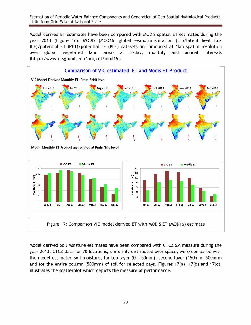
Figure 17: Comparison VIC model derived ET with MODIS ET (MOD16) estimate 29
Figure 18: Comparison of is Field observed field SM with VIC modeled SM on a day with rainfall distributed uniformly over space
30
Figure 19: Comparison of is Field observed field SM with VIC modeled SM on a day with localized rainfall occurrences
31
Figure 20: Comparison of trend in SM variation from June to October (Modeled and Field observed) in at Station 1
32
Figure 21: Comparison of trend in SM variation from June to October (Modeled and Field observed) in at Station 2
33
Figure 22: Long-term hydrological fluxes estimated at 9min grid level for the entire country
35

v
Figure 23: Seasonal water balance components (Jun-Oct) during 2013 and 2014 as estimated
from hydrological modeling
36
Figure 24: Daily water balance components published on Bhuvan web portal 37
Figure 25: Standardized Runoff Index generated from the hydrological model outputs
38
Figure 26: 3min Grid level water balance components 40
Figure 27: Hydrological model (3min) derivatives for Mahanadi river basin 41
Estimation of Periodic Water Balance Components and Generation of Geo-Spatial Hydrological
Products at Uniform Grid-Wise at National Scale
1
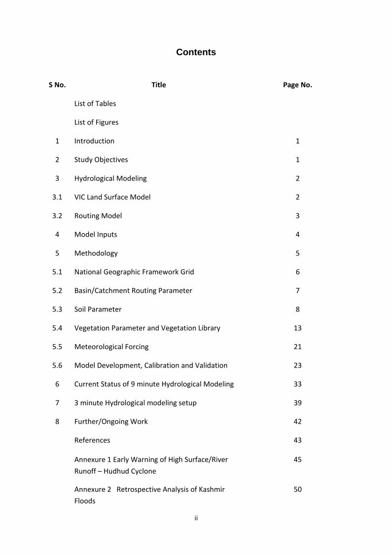
1 INTRODUCTION
Description of terrestrial water flux components in terms of their geographical distribution
and chronological variation is useful for water resources assessment, management and
climate related research. Water resources availability and its controlling parameters are
spatially distributed and show significant temporal variability. Hydrological response has a
functional dependency of many dynamic and stationary parameters. Spatial heterogeneity
and time variant behavior of these parameters are critical inputs into Hydrological models.
Earth Observation (EO) data from multitude platforms providing enormous contribution for
the creation of spatially distributed parameters relevant for hydrological budgeting and
modeling. Repeatability of observations allows the generation of a time-series account of
dynamic terrain parameters and provides capability to quantify and forecast the
hydrological variables and water balance components.
The EOAM study being executed under Earth Observation Application Mission (EOAM)
programme of ISRO. The objective is to establish a national level hybrid modelling
framework, where the major hydrological processes are modeled through integration of
geo-spatial data sets with hydro-meteorological data. The diverse modules are based on
conceptual, empirical and process based approaches. The focus is on quantifying the
spatial and temporal distribution of water balance components and to provide orderly
description hydrological fluxes through geo-spatial products at regular periodicity. The
model derived fluxes are useful for quantifying spatial and temporal variation in
basin/sub-basin scale water resources, periodical water budgeting and form vital inputs
for studies on topics ranging from water resources management to land-atmosphere
interactions including climate change.
2 STUDY OBJECTIVES
The scope of the study is to generate grid-wise periodic water balance components at
using distributed hydrological modelling using geo-spatial and hydro-meteorological data.
The specific objectives are
I. To develop and setup frame work for generation of grid-wise, water balance
components covering all the river basins of the country using geo-spatial and
hydro-meteorological data sets using macro-scale hydrological model
II. To conduct field experimentation for calibration and validation of model outputs
III. To generate periodic geo-spatial products describing grid-wise water balance
components for the entire country

Estimation of Periodic Water Balance Components and Generation of Geo-Spatial Hydrological
Products at Uniform Grid-Wise at National Scale
2
3 HYDROLOGICAL MODEL
Among the many hydrological models developed world wide, Variable Infiltration Capacity
(VIC) model is extensively used by earth observation scientific fraternity for its methodical
rationale, inclusion of bio-physical processes that govern water-energy exchanges and
adoptability to different regions. VIC model is extensively used in studies on topics ranging
from water resources management to land-atmosphere interactions and climate change.
3.1 VIC Land Surface Model
The Variable Infiltration Capacity (VIC), a semi distributed & physically based hydrological
model that solves both the water balance and the energy balance (Figure 1). VIC is an
open source research model, its various forms has been applied to many watersheds
including the Fraser River, Columbia River, the Ohio River, the Arkansas-Red Rivers, and
the Upper Mississippi Rivers. Employing the infiltration and surface runoff scheme in
Xianjiang model (Zhao, 1980), VIC was first described as a single soil layer model by
(Wood, 1992) and implemented in the GFDL and Max-Planck-Institute (MPI) GCMs.
Figure 1: Schematic representation of VIC hydrological model
VIC is capable of partitioning incoming (solar and long wave) radiation at the land surface
into latent and sensible heat, and the partitioning of precipitation (or snowmelt) into
direct runoff and infiltration. It utilizes a soil–vegetation–atmosphere transfer scheme that
accounts for the influence of vegetation and soil moisture on land–atmosphere
interactions. The model handles the subsurface into multiple soil layers. Each layer
characterizes soil hydrological response such as bulk density, infiltration capacity,
saturated hydraulic conductivity, soil layer depths, and soil moisture diffusion parameters.

Estimation of Periodic Water Balance Components and Generation of Geo-Spatial Hydrological
Products at Uniform Grid-Wise at National Scale
3
VIC explicitly represents sub-grid heterogeneity in land cover classes taking their
phenological changes into account such as their leaf area index (LAI), albedo, canopy
resistance, and relative fraction of roots in each of the soil layers. The evapotranspiration
from each land cover type is simulated using vegetation-class specific potential
evapotranspiration, canopy resistance, aerodynamic resistance to the transport of water,
and architectural resistance coefficients as defined in Penman-Monteith equation. In this
model, the ET includes evaporation from the canopy layer of each vegetation class,
transpiration from each vegetation class, and evaporation from bare soil. Total
evapotranspiration ET over each grid cell is calculated as the area weighted sum of these
three components. VIC uses the infiltration mechanism used in Xinanjang model (Zhao,
1992) to generate runoff from precipitation in excess of available infiltration capacity and
base flow is computed using Arno model conceptualization (Todini, 1996).
In the model, soil moisture distribution, infiltration, drainage between soil layers, surface
runoff, and subsurface runoff are all calculated for each land cover tile at each time step.
Then for each grid cell, the total heat fluxes (latent heat, sensible heat, and ground
heat), effective surface temperature, and the total surface and subsurface runoff are
obtained by summing over all the land cover tiles weighted by fractional coverage.
Routing Model
In the VIC model, each grid cell is modeled independently without horizontal water flow.
The grid-based VIC model simulates the time series of runoff only for each grid cell, which
is non-uniformly distributed within the cell. In the routing model, water is never allowed
to flow from the channel back into the grid cell. Once it reaches the channel, it is no
longer part of the water budget. A linear transfer function model characterized by its
internal impulse response function is used to calculate the within-cell routing. Then by
assuming all runoff exits a cell in a single flow direction, a channel routing based on the
linearized Saint-Venant equation is used to simulate the discharge at the basin outlet
(Figure 2). The routing model is described in detail by Lohmann et al. (1996, 1998a).

Estimation of Periodic Water Balance Components and Generation of Geo-Spatial Hydrological
Products at Uniform Grid-Wise at National Scale
4
Figure 2: Schematic representation of VIC Routing model
4 MODEL INPUTS
The VIC model requires several sets of input data and are broadly categorized into:
1. Meteorological Forcing Files: VIC can take daily or sub-daily time-series of
meteorological variables as inputs for each grid separately
2. Soil Parameter File: The soil parameter predominantly defines the grid-wise,
layer-wise soil hydraulic particulars and along with model control parameters.
The soil hydraulic parameters include saturated hydraulic conductivity, density,
maximum soil moisture holding capacity, etc.
3. Vegetation Parameter & Library File: Land cover types, fractional areas, rooting
depths, and seasonal LAIs of the various land cover tiles within each grid cell.
4. Global Parameter File: This is the main input file for VIC. It points VIC to the
locations of the other input/output files and sets parameters that govern the
simulation and model run
5. Routing Parameter File: Grid-wise elevation, direction of flow, slope, catchment
fraction, diffusion
Using the various geo-spatial data sources (Table 1), model specific inputs have been
prepared for the entire country and are detailed in the Methodology section.

Estimation of Periodic Water Balance Components and Generation of Geo-Spatial Hydrological
Products at Uniform Grid-Wise at National Scale
5
Table 1 Data sets are used for generating the model specific inputs
S. No. Parameter Data sources
1 Terrain Carosat-1 DEM
Aster DEM
SRTM DEM
2 Soil NBSS & LUP Soil Map of India (1:500,000 scale)
FAO Soil data series (5 Million scale)
Field data / Literature / Experimentation
3 Vegetation Library LAI, Albedo (MODIS / NPOESS / JPSS)
Physical parameters (Field data / Literature /
Experimentation)
4 Vegetation cover LULC (NRC-250k)
5 Irrigation Irrigation command maps (India-WRIS)
6 Meteorological data IMD surface / Gridded data (historic, Real-time,
and forecast)
IMD / ISRO AWS
Satellite meteorological products (TRMM, CPC,
MOSDAC, ...)
7 River discharge CWC River discharge data (Historic/real-time)
8 Reservoir data Storage, Rating curves, Releases
5 METHODOLOGY
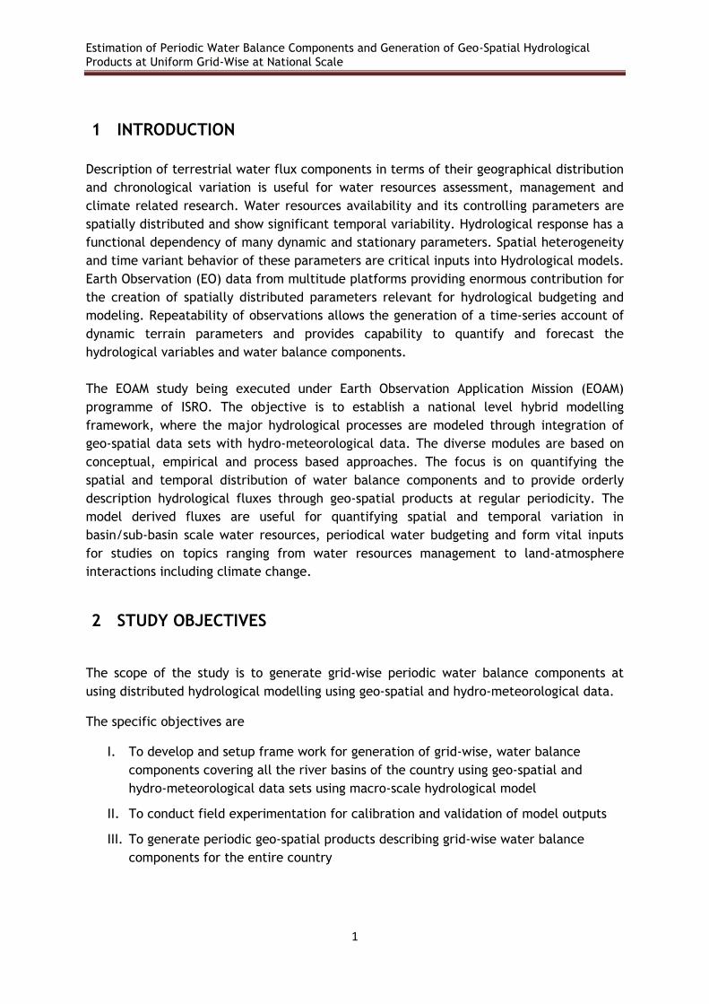
Brief methodological steps (Figure 3) involved are as under:
• Geographical framework setup at 9min (~16.5km) grid level
• Catchment delineation for CWC Discharge sites using DEM
• Preparation Routing Parameters file (grid-wise fraction, flow direction)
• Preparation of model specific parameters on Soil, Vegetation and Routing using
geo-spatial data sets (DEM, Land Use/Land Cover, Soil, Albedo, LAI, etc.)
• Preparation Soil Parameter file for each catchment (soil type, layer-wise depth,
hydraulic properties)
• Preparation of vegetation parameter (Vegetation type, fraction)
• Preparation of Vegetation library (Monthly LAI, Albedo, Canopy resistance factors,
Displacement height)
• Meteorological forcing data preparation and generation grid-wise forcing data Ascii
files
• VIC Model setup and Run
Estimation of Periodic Water Balance Components and Generation of Geo-Spatial Hydrological
Products at Uniform Grid-Wise at National Scale
6
• Routing Model Run
• Calibration of simulated discharge with observed discharge for selected historic
years
• Model computations with calibrated parameterization using historic climate data
and in-season climate data
• Generation of grid-wise daily water balance components
• Integration and Conversion of grid-wise VIC outputs into geo-spatial data sets /
products and web publishing
Figure 3: Methodological framework of VIC Hydrological modelling
5.1 National Geographic Framework Grid
The entire VIC model operations are grid-centric, with each grid is independently handled
for water/energy balance computations. The various parameters (soil, vegetation,
meteorological, routing) are indexed through grid unique numbering and sub-routines
perform the required computations through reading various parameter files.
Estimation of Periodic Water Balance Components and Generation of Geo-Spatial Hydrological
Products at Uniform Grid-Wise at National Scale
7
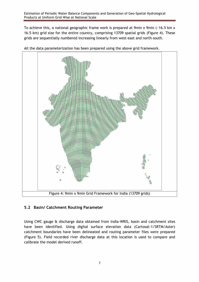
To achieve this, a national geographic frame work is prepared at 9min x 9min (~16.5 km x
16.5 km) grid size for the entire country, comprising 13709 spatial grids (Figure 4). These
grids are sequentially numbered increasing linearly from west-east and north-south.
All the data parameterization has been prepared using the above grid framework.
Figure 4: 9min x 9min Grid Framework for India (13709 grids)
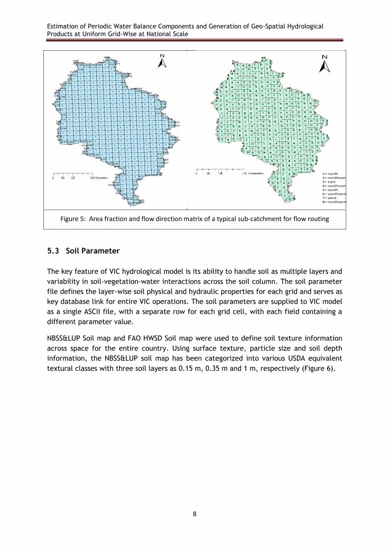
5.2 Basin/ Catchment Routing Parameter
Using CWC gauge & discharge data obtained from India-WRIS, basin and catchment sites
have been identified. Using digital surface elevation data (Cartosat-1/SRTM/Aster)
catchment boundaries have been delineated and routing parameter files were prepared
(Figure 5). Field recorded river discharge data at this location is used to compare and
calibrate the model derived runoff.
Estimation of Periodic Water Balance Components and Generation of Geo-Spatial Hydrological
Products at Uniform Grid-Wise at National Scale
8
Figure 5: Area fraction and flow direction matrix of a typical sub-catchment for flow routing
5.3 Soil Parameter
The key feature of VIC hydrological model is its ability to handle soil as multiple layers and
variability in soil-vegetation-water interactions across the soil column. The soil parameter
file defines the layer-wise soil physical and hydraulic properties for each grid and serves as
key database link for entire VIC operations. The soil parameters are supplied to VIC model
as a single ASCII file, with a separate row for each grid cell, with each field containing a
different parameter value.
NBSS&LUP Soil map and FAO HWSD Soil map were used to define soil texture information
across space for the entire country. Using surface texture, particle size and soil depth
information, the NBSS&LUP soil map has been categorized into various USDA equivalent
textural classes with three soil layers as 0.15 m, 0.35 m and 1 m, respectively (Figure 6).
1= north2= northeast3= east4= southeast5= south6= southwest7= west8= northwest

Estimation of Periodic Water Balance Components and Generation of Geo-Spatial Hydrological Products at Uniform Grid-Wise at National Scale
9
Layer 1 (0-15 cm) Layer 2 (15-50 cm) Layer 3 (50-150 cm)
Figure 6: Soil Textural Map (USDA Class) used for the Study
Estimation of Periodic Water Balance Components and Generation of Geo-Spatial Hydrological Products
at Uniform Grid-Wise at National Scale
10
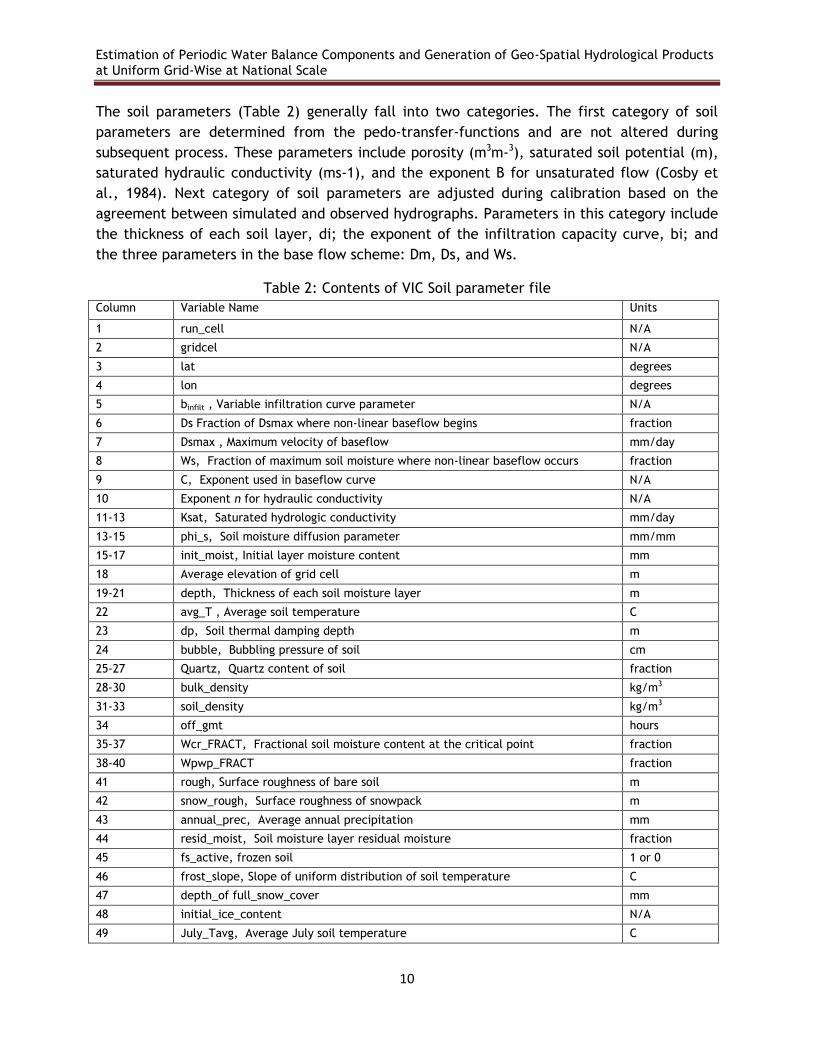
The soil parameters (Table 2) generally fall into two categories. The first category of soil
parameters are determined from the pedo-transfer-functions and are not altered during
subsequent process. These parameters include porosity (m3m-3), saturated soil potential (m),
saturated hydraulic conductivity (ms-1), and the exponent B for unsaturated flow (Cosby et
al., 1984). Next category of soil parameters are adjusted during calibration based on the
agreement between simulated and observed hydrographs. Parameters in this category include
the thickness of each soil layer, di; the exponent of the infiltration capacity curve, bi; and
the three parameters in the base flow scheme: Dm, Ds, and Ws.
Table 2: Contents of VIC Soil parameter file
Column Variable Name Units
1 run_cell N/A
2 gridcel N/A
3 lat degrees
4 lon degrees
5 binfilt , Variable infiltration curve parameter N/A
6 Ds Fraction of Dsmax where non-linear baseflow begins fraction
7 Dsmax , Maximum velocity of baseflow mm/day
8 Ws, Fraction of maximum soil moisture where non-linear baseflow occurs fraction
9 C, Exponent used in baseflow curve N/A
10 Exponent n for hydraulic conductivity N/A
11-13 Ksat, Saturated hydrologic conductivity mm/day
13-15 phi_s, Soil moisture diffusion parameter mm/mm
15-17 init_moist, Initial layer moisture content mm
18 Average elevation of grid cell m
19-21 depth, Thickness of each soil moisture layer m
22 avg_T , Average soil temperature C
23 dp, Soil thermal damping depth m
24 bubble, Bubbling pressure of soil cm
25-27 Quartz, Quartz content of soil fraction
28-30 bulk_density kg/m3
31-33 soil_density kg/m3
34 off_gmt hours
35-37 Wcr_FRACT, Fractional soil moisture content at the critical point fraction
38-40 Wpwp_FRACT fraction
41 rough, Surface roughness of bare soil m
42 snow_rough, Surface roughness of snowpack m
43 annual_prec, Average annual precipitation mm
44 resid_moist, Soil moisture layer residual moisture fraction
45 fs_active, frozen soil 1 or 0
46 frost_slope, Slope of uniform distribution of soil temperature C
47 depth_of full_snow_cover mm
48 initial_ice_content N/A
49 July_Tavg, Average July soil temperature C
Estimation of Periodic Water Balance Components and Generation of Geo-Spatial Hydrological Products
at Uniform Grid-Wise at National Scale
11
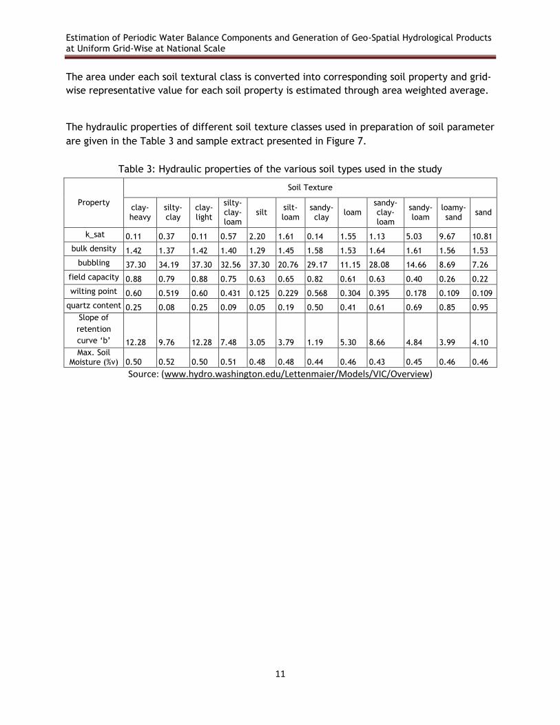
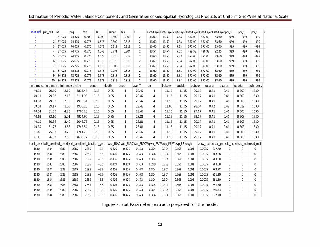
The area under each soil textural class is converted into corresponding soil property and grid-
wise representative value for each soil property is estimated through area weighted average.
The hydraulic properties of different soil texture classes used in preparation of soil parameter
are given in the Table 3 and sample extract presented in Figure 7.
Table 3: Hydraulic properties of the various soil types used in the study
Property
Soil Texture
clay-heavy
silty-clay
clay-light
silty-clay-loam
silt silt-loam
sandy-clay
loam sandy-clay-loam
sandy-loam
loamy-sand
sand
k_sat 0.11 0.37 0.11 0.57 2.20 1.61 0.14 1.55 1.13 5.03 9.67 10.81
bulk density 1.42 1.37 1.42 1.40 1.29 1.45 1.58 1.53 1.64 1.61 1.56 1.53
bubbling 37.30 34.19 37.30 32.56 37.30 20.76 29.17 11.15 28.08 14.66 8.69 7.26
field capacity 0.88 0.79 0.88 0.75 0.63 0.65 0.82 0.61 0.63 0.40 0.26 0.22
wilting point 0.60 0.519 0.60 0.431 0.125 0.229 0.568 0.304 0.395 0.178 0.109 0.109
quartz content 0.25 0.08 0.25 0.09 0.05 0.19 0.50 0.41 0.61 0.69 0.85 0.95
Slope of
retention
curve ‘b’ 12.28 9.76 12.28 7.48 3.05 3.79 1.19 5.30 8.66 4.84 3.99 4.10
Max. Soil Moisture (%v) 0.50 0.52 0.50 0.51 0.48 0.48 0.44 0.46 0.43 0.45 0.46 0.46
Source: (www.hydro.washington.edu/Lettenmaier/Models/VIC/Overview)
Estimation of Periodic Water Balance Components and Generation of Geo-Spatial Hydrological Products at Uniform Grid-Wise at National Scale
12
Figure 7: Soil Parameter (extract) prepared for the model
#run_cell grid_cell lat long infilt Ds Dsmax Ws c expt-Layer1expt-Layer2expt-Layer3Ksat-Layer1Ksat-Layer2Ksat-Layer3phi_s phi_s phi_s init_moist init_moist init_moist elev depth depth depth avg_T dp bubble bubble bubble quartz quartz quartz bulk_density (kg/m3)bulk_density (kg/m3)bulk_density (kg/m3)soil_density soil_density soil_density off_gmt Wcr_FRACT Wcr_FRACT Wcr_FRACT Wpwp_FRACTWpwp_FRACTWpwp_FRACTrough snow_roughannual_precresid_moist resid_moist resid_moist fs_active frost_slopedepth_full_snow_coverinitial_ice_contentJuly_Tavg
1 1 37.025 74.325 0.300 0.000 0.309 0.000 2 13.60 13.60 5.38 372.00 372.00 33.60 -999 -999 -999 40.31 79.69 2.19 4833.45 0.15 0.35 1 29.42 4 11.15 11.15 29.17 0.41 0.41 0.503 1530 1530 1584 2685 2685 2685 +5.5 0.426 0.426 0.573 0.304 0.304 0.568 0.001 0.0005 637.70 0 0 0 0
1 2 37.025 74.475 0.275 0.573 0.309 0.818 2 13.60 13.60 5.38 372.00 372.00 33.60 -999 -999 -999 40.11 79.32 2.16 5111.93 0.15 0.35 1 29.42 4 11.15 11.15 29.17 0.41 0.41 0.503 1530 1530 1584 2685 2685 2685 +5.5 0.426 0.426 0.573 0.304 0.304 0.568 0.001 0.0005 763.58 0 0 0 0
1 3 37.025 74.625 0.275 0.573 0.312 0.818 2 13.60 13.60 5.38 372.00 372.00 33.60 -999 -999 -999 40.33 79.82 2.50 4976.31 0.15 0.35 1 29.42 4 11.15 11.15 29.17 0.41 0.41 0.503 1530 1530 1584 2685 2685 2685 +5.5 0.426 0.426 0.573 0.304 0.304 0.568 0.001 0.0005 763.58 0 0 0 0
1 4 37.025 74.775 0.275 0.563 0.781 0.804 2 13.54 13.54 5.52 428.98 428.98 92.25 -999 -999 -999 39.33 79.17 1.60 4920.28 0.15 0.35 1 29.42 4 11.05 11.05 28.64 0.42 0.42 0.512 1530 1530 1583 2685 2685 2685 +5.5 0.419 0.419 0.563 0.299 0.299 0.556 0.001 0.0005 763.58 0 0 0 0
1 5 37.025 74.925 0.275 0.573 0.326 0.818 2 13.60 13.60 5.38 372.00 372.00 33.60 -999 -999 -999 40.54 81.65 4.93 4760.28 0.15 0.35 1 29.42 4 11.15 11.15 29.17 0.41 0.41 0.503 1530 1530 1584 2685 2685 2685 +5.5 0.426 0.426 0.573 0.304 0.304 0.568 0.001 0.0005 763.58 0 0 0 0
1 6 37.025 75.075 0.275 0.573 0.326 0.818 2 13.60 13.60 5.38 372.00 372.00 33.60 -999 -999 -999 40.69 82.10 5.01 4924.90 0.15 0.35 1 28.86 4 11.15 11.15 29.17 0.41 0.41 0.503 1530 1530 1584 2685 2685 2685 +5.5 0.426 0.426 0.573 0.304 0.304 0.568 0.001 0.0005 851.30 0 0 0 0
1 7 37.025 75.225 0.275 0.573 0.308 0.818 2 13.60 13.60 5.38 372.00 372.00 33.60 -999 -999 -999 40.19 80.84 3.40 5046.75 0.15 0.35 1 28.86 4 11.15 11.15 29.17 0.41 0.41 0.503 1530 1530 1584 2685 2685 2685 +5.5 0.426 0.426 0.573 0.304 0.304 0.568 0.001 0.0005 851.30 0 0 0 0
1 8 37.025 75.375 0.275 0.573 0.295 0.818 2 13.60 13.60 5.38 372.00 372.00 33.60 -999 -999 -999 40.39 81.77 3.86 4745.54 0.15 0.35 1 28.86 4 11.15 11.15 29.17 0.41 0.41 0.503 1530 1530 1584 2685 2685 2685 +5.5 0.426 0.426 0.573 0.304 0.304 0.568 0.001 0.0005 851.30 0 0 0 0
1 9 36.875 73.725 0.275 0.573 0.318 0.818 2 13.60 13.60 5.38 372.00 372.00 33.60 -999 -999 -999 0.02 75.97 3.79 4761.78 0.15 0.35 1 29.42 4 11.15 11.15 29.17 0.41 0.41 0.503 1530 1530 1584 2685 2685 2685 +5.5 0.426 0.426 0.573 0.304 0.304 0.568 0.001 0.0005 390.33 0 0 0 0
1 10 36.875 73.875 0.275 0.573 0.336 0.818 2 13.60 13.60 5.38 372.00 372.00 33.60 -999 -999 -999 0.03 76.33 2.89 4630.72 0.15 0.35 1 29.42 4 11.15 11.15 29.17 0.41 0.41 0.503 1530 1530 1584 2685 2685 2685 +5.5 0.426 0.426 0.573 0.304 0.304 0.568 0.001 0.0005 637.70 0 0 0 0
Estimation of Periodic Water Balance Components and Generation of Geo-Spatial Hydrological Products
at Uniform Grid-Wise at National Scale
13
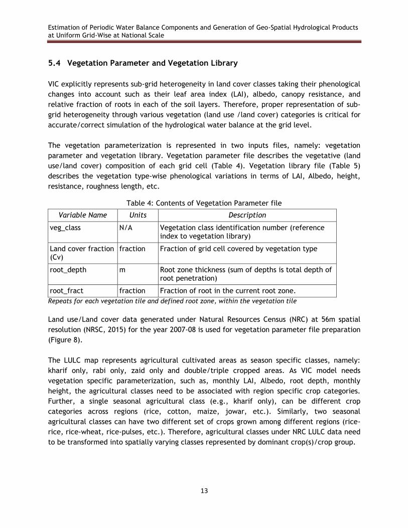
5.4 Vegetation Parameter and Vegetation Library
VIC explicitly represents sub-grid heterogeneity in land cover classes taking their phenological
changes into account such as their leaf area index (LAI), albedo, canopy resistance, and
relative fraction of roots in each of the soil layers. Therefore, proper representation of sub-
grid heterogeneity through various vegetation (land use /land cover) categories is critical for
accurate/correct simulation of the hydrological water balance at the grid level.
The vegetation parameterization is represented in two inputs files, namely: vegetation
parameter and vegetation library. Vegetation parameter file describes the vegetative (land
use/land cover) composition of each grid cell (Table 4). Vegetation library file (Table 5)
describes the vegetation type-wise phenological variations in terms of LAI, Albedo, height,
resistance, roughness length, etc.
Table 4: Contents of Vegetation Parameter file
Variable Name Units Description
veg_class N/A Vegetation class identification number (reference index to vegetation library)
Land cover fraction (Cv)
fraction Fraction of grid cell covered by vegetation type
root_depth m Root zone thickness (sum of depths is total depth of root penetration)
root_fract fraction Fraction of root in the current root zone.
Repeats for each vegetation tile and defined root zone, within the vegetation tile
Land use/Land cover data generated under Natural Resources Census (NRC) at 56m spatial
resolution (NRSC, 2015) for the year 2007-08 is used for vegetation parameter file preparation
(Figure 8).
The LULC map represents agricultural cultivated areas as season specific classes, namely:
kharif only, rabi only, zaid only and double/triple cropped areas. As VIC model needs
vegetation specific parameterization, such as, monthly LAI, Albedo, root depth, monthly
height, the agricultural classes need to be associated with region specific crop categories.
Further, a single seasonal agricultural class (e.g., kharif only), can be different crop
categories across regions (rice, cotton, maize, jowar, etc.). Similarly, two seasonal
agricultural classes can have two different set of crops grown among different regions (rice-
rice, rice-wheat, rice-pulses, etc.). Therefore, agricultural classes under NRC LULC data need
to be transformed into spatially varying classes represented by dominant crop(s)/crop group.

Estimation of Periodic Water Balance Components and Generation of Geo-Spatial Hydrological Products
at Uniform Grid-Wise at National Scale
14
Figure 8: Land use/Land cover map – Year 2007-08
(source: NRSC)
Leaf area index (LAI) is dimensionless and is defined as the one sided green leaf area per unit
ground area. Vegetation, specifically agricultural crops, exhibit significant seasonal and intra-
seasonal variation in LAI resulting from type, growth stage and seasonal variations. Son et. al.
(2014) demonstrated the usefulness of phenology-based classification approach to derive
information of rice growing areas. Global products of vegetation green Leaf Area
Index (LAI) are being operationally produced from Terra and Aqua Moderate Resolution
Imaging Spectroradiometer (MODIS) at 1-km resolution and eight-day frequency (MOD15A2;
www.modisland.gsfc.nasa.gov)
2007-08 year 8-day LAI data were downloaded for Indian region and time-series stacked image
was prepared. Using the agricultural mask from LULC map, the time-series LAI stacked image
was categorized into multiple classes representing spatially and temporally varying LAI
profiles using iso-data clustering technique. By comparing with field district/state
agricultural statistics, LAI classes were related with agricultural crop dominant areas and
entire agricultural area has been converted into major/dominant crop type map. The
schematic representation of the above approach is presented Figure 9.

Estimation of Periodic Water Balance Components and Generation of Geo-Spatial Hydrological Products
at Uniform Grid-Wise at National Scale
15
Figure 9: Reclassification of LULC agricultural area into crop specific dominant areas using
time-series LAI data
The other land use/land cover classes (forest, water bodies, urban, etc.) were adopted
directly from LULC map and an integrated vegetation map has been prepared for 2007-08 year
(Figure 10). This exercise enabled improved definition of vegetation parameterization for
entire India, incorporating the region specific crop parameterization.
Using 9min grid shape file and vegetation map, 9min grid-wise vegetation composition is
extracted to arrive at model specific vegetation parameter file (Figure 11).

Estimation of Periodic Water Balance Components and Generation of Geo-Spatial Hydrological Products
at Uniform Grid-Wise at National Scale
16
Legend
Figure 10: Integrated vegetation (LULC and Crop Type) – Year 2007-08
Build up Plantation/orchard Evergreen forest Deciduous forest Scrub/Deg. forest Littoral swamp Grassland Other wasteland Gullied Scrubland Water bodies Snow covered Rann Cotton-Wheat Rice-Wheat(pnb) Rice-Wheat(UP) Rice-Rice Rice Maize/Bajra Soyabean Rice Aman Paddy Bajra Jowar Coconut Rice(TN) Ragi
Legend
india_state_new
0
1
2
3
4
5
6
7
8
9
10
11
12
13
14
15
16
17
18
19
20
21
22
23
24
25
26
27
28
29
30
31
32
33
34
Legend
india_state_new
0
1
2
3
4
5
6
7
8
9
10
11
12
13
14
15
16
17
18
19
20
21
22
23
24
25
26
27
28
29
30
31
32
33
34
Legend
india_state_new
0
1
2
3
4
5
6
7
8
9
10
11
12
13
14
15
16
17
18
19
20
21
22
23
24
25
26
27
28
29
30
31
32
33
34
Legend
india_state_new
0
1
2
3
4
5
6
7
8
9
10
11
12
13
14
15
16
17
18
19
20
21
22
23
24
25
26
27
28
29
30
31
32
33
34

Estimation of Periodic Water Balance Components and Generation of Geo-Spatial Hydrological Products
at Uniform Grid-Wise at National Scale
17
1 4
1 0.5915 0.150 0.250 0.350 0.650 1.000 0.100
13 0.0628 0.150 0.200 0.350 0.600 1.000 0.200
16 0.0693 0.150 0.600 0.350 0.400 1.000 0.000
19 0.2763 0.150 0.400 0.350 0.500 1.000 0.100
2 4
1 0.2787 0.150 0.250 0.350 0.650 1.000 0.100
4 0.1519 0.150 0.600 0.350 0.300 1.000 0.100
5 0.0730 0.150 0.600 0.350 0.300 1.000 0.100
19 0.4964 0.150 0.400 0.350 0.500 1.000 0.100
3 4
1 0.3496 0.150 0.250 0.350 0.650 1.000 0.100
3 0.0563 0.150 0.250 0.350 0.600 1.000 0.150
4 0.0617 0.150 0.600 0.350 0.300 1.000 0.100
19 0.5325 0.150 0.400 0.350 0.500 1.000 0.100
4 4
1 0.2072 0.150 0.250 0.350 0.650 1.000 0.100
16 0.1126 0.150 0.600 0.350 0.400 1.000 0.000
18 0.0797 0.150 0.200 0.350 0.600 1.000 0.200
19 0.6004 0.150 0.400 0.350 0.500 1.000 0.100
5 5
1 0.0901 0.150 0.250 0.350 0.650 1.000 0.100
4 0.0691 0.150 0.600 0.350 0.300 1.000 0.100
16 0.1874 0.150 0.600 0.350 0.400 1.000 0.000
18 0.3194 0.150 0.200 0.350 0.600 1.000 0.200
19 0.3340 0.150 0.400 0.350 0.500 1.000 0.100
6 4
1 0.0826 0.150 0.250 0.350 0.650 1.000 0.100
5 0.1127 0.150 0.600 0.350 0.300 1.000 0.100
18 0.6545 0.150 0.200 0.350 0.600 1.000 0.200
19 0.1502 0.150 0.400 0.350 0.500 1.000 0.100
7 2
1 0.7626 0.150 0.250 0.350 0.650 1.000 0.100
16 0.2374 0.150 0.600 0.350 0.400 1.000 0.000
8 4
1 0.6209 0.150 0.250 0.350 0.650 1.000 0.100
4 0.0527 0.150 0.600 0.350 0.300 1.000 0.100
16 0.0981 0.150 0.600 0.350 0.400 1.000 0.000
19 0.2283 0.150 0.400 0.350 0.500 1.000 0.100
9 3
1 0.6153 0.150 0.250 0.350 0.650 1.000 0.100
16 0.0776 0.150 0.600 0.350 0.400 1.000 0.000
19 0.3071 0.150 0.400 0.350 0.500 1.000 0.100
10 3
1 0.2677 0.150 0.250 0.350 0.650 1.000 0.100
16 0.2306 0.150 0.600 0.350 0.400 1.000 0.000
19 0.5017 0.150 0.400 0.350 0.500 1.000 0.100
Figure 11: Extract of Vegetation Parameter file prepared for the model
Estimation of Periodic Water Balance Components and Generation of Geo-Spatial Hydrological Products
at Uniform Grid-Wise at National Scale
18
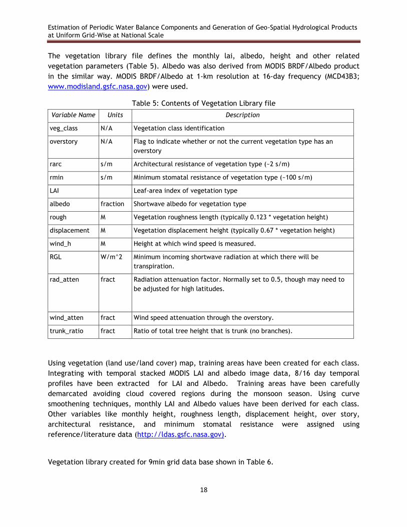
The vegetation library file defines the monthly lai, albedo, height and other related
vegetation parameters (Table 5). Albedo was also derived from MODIS BRDF/Albedo product
in the similar way. MODIS BRDF/Albedo at 1-km resolution at 16-day frequency (MCD43B3;
www.modisland.gsfc.nasa.gov) were used.
Table 5: Contents of Vegetation Library file
Variable Name Units Description
veg_class N/A Vegetation class identification
overstory N/A Flag to indicate whether or not the current vegetation type has an
overstory
rarc s/m Architectural resistance of vegetation type (~2 s/m)
rmin s/m Minimum stomatal resistance of vegetation type (~100 s/m)
LAI Leaf-area index of vegetation type
albedo fraction Shortwave albedo for vegetation type
rough M Vegetation roughness length (typically 0.123 * vegetation height)
displacement M Vegetation displacement height (typically 0.67 * vegetation height)
wind_h M Height at which wind speed is measured.
RGL W/m^2 Minimum incoming shortwave radiation at which there will be
transpiration.
rad_atten fract Radiation attenuation factor. Normally set to 0.5, though may need to
be adjusted for high latitudes.
wind_atten fract Wind speed attenuation through the overstory.
trunk_ratio fract Ratio of total tree height that is trunk (no branches).
Using vegetation (land use/land cover) map, training areas have been created for each class.
Integrating with temporal stacked MODIS LAI and albedo image data, 8/16 day temporal
profiles have been extracted for LAI and Albedo. Training areas have been carefully
demarcated avoiding cloud covered regions during the monsoon season. Using curve
smoothening techniques, monthly LAI and Albedo values have been derived for each class.
Other variables like monthly height, roughness length, displacement height, over story,
architectural resistance, and minimum stomatal resistance were assigned using
reference/literature data (http://ldas.gsfc.nasa.gov).
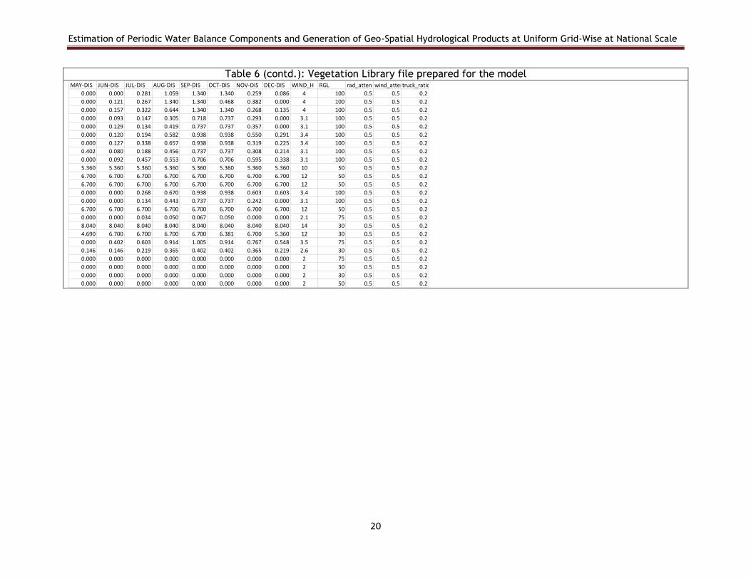
Vegetation library created for 9min grid data base shown in Table 6.

Estimation of Periodic Water Balance Components and Generation of Geo-Spatial Hydrological Products at Uniform Grid-Wise at National Scale
19
Table 6: Vegetation Library file prepared for the model
#Class OvrStry Rarc Rmin JAN-LAI FEB-LAI MAR-LAI APR-LAI MAY-LAI JUN-LAI JUL-LAI AUG-LAI SEP-LAI OCT-LAI NOV-LAI DEC-LAI JAN-ALB FEB_ALB MAR-ALB APR-ALB MAY-ALB JUN-ALB JUL-ALB AUG-ALB SEP-ALB OCT-ALB NOV-ALB DEC-ALB JAN-ROU FEB-ROU MAR-ROU APR-ROU MAY-ROU JUN-ROU JUL-ROU AUG-ROU SEP-ROU OCT-ROU NOV-ROU DEC-ROU JAN-DIS FEB-DIS MAR-DIS APR-DIS MAY-DIS JUN-DIS JUL-DIS AUG-DIS SEP-DIS OCT-DIS NOV-DIS DEC-DIS WIND_H RGL rad_atten wind_attentruck_ratio
1 0 25 80 0.00 0.00 0.00 0.00 0.00 0.00 0.65 2.45 3.10 1.35 0.60 0.20 0.160 0.160 0.160 0.160 0.160 0.139 0.128 0.125 0.124 0.136 0.148 0.160 0.000 0.000 0.000 0.000 0.000 0.000 0.052 0.194 0.246 0.246 0.048 0.016 0.000 0.000 0.000 0.000 0.000 0.000 0.281 1.059 1.340 1.340 0.259 0.086 4 100 0.5 0.5 0.2
2 0 25 80 0.00 0.00 0.00 0.00 0.00 0.27 0.60 3.01 2.26 1.05 0.86 0.00 0.142 0.141 0.140 0.140 0.140 0.120 0.115 0.115 0.122 0.135 0.135 0.140 0.000 0.000 0.000 0.000 0.000 0.022 0.049 0.246 0.246 0.086 0.070 0.000 0.000 0.000 0.000 0.000 0.000 0.121 0.267 1.340 1.340 0.468 0.382 0.000 4 100 0.5 0.5 0.2
3 0 25 80 0.00 0.00 0.00 0.00 0.00 0.27 0.55 1.10 2.09 2.29 1.15 0.23 0.152 0.148 0.148 0.148 0.148 0.118 0.115 0.115 0.115 0.130 0.139 0.145 0.000 0.000 0.000 0.000 0.000 0.029 0.059 0.118 0.246 0.246 0.049 0.025 0.000 0.000 0.000 0.000 0.000 0.157 0.322 0.644 1.340 1.340 0.268 0.135 4 100 0.5 0.5 0.2
4 0 25 80 0.00 0.00 0.00 0.00 0.00 0.38 0.60 1.25 2.94 3.02 1.20 0.00 0.145 0.141 0.141 0.145 0.145 0.130 0.110 0.110 0.110 0.120 0.130 0.143 0.000 0.000 0.000 0.000 0.000 0.017 0.027 0.056 0.132 0.135 0.054 0.000 0.000 0.000 0.000 0.000 0.000 0.093 0.147 0.305 0.718 0.737 0.293 0.000 3.1 100 0.5 0.5 0.2
5 0 25 80 0.00 0.00 0.00 0.00 0.00 0.61 0.95 2.00 3.51 3.15 1.70 0.00 0.137 0.137 0.137 0.137 0.144 0.130 0.105 0.100 0.100 0.110 0.135 0.137 0.000 0.000 0.000 0.000 0.000 0.024 0.025 0.077 0.135 0.135 0.065 0.000 0.000 0.000 0.000 0.000 0.000 0.129 0.134 0.419 0.737 0.737 0.357 0.000 3.1 100 0.5 0.5 0.2
6 0 25 80 0.00 0.00 0.00 0.00 0.00 0.37 0.60 1.80 2.45 2.90 1.70 0.90 0.159 0.150 0.149 0.150 0.150 0.135 0.125 0.120 0.120 0.120 0.140 0.158 0.000 0.000 0.000 0.000 0.000 0.022 0.036 0.107 0.172 0.172 0.101 0.053 0.000 0.000 0.000 0.000 0.000 0.120 0.194 0.582 0.938 0.938 0.550 0.291 3.4 100 0.5 0.5 0.2
7 0 25 80 0.00 0.00 0.00 0.00 0.00 0.34 0.90 1.75 2.25 2.50 0.85 0.60 0.151 0.150 0.150 0.150 0.150 0.130 0.120 0.120 0.120 0.120 0.147 0.151 0.000 0.000 0.000 0.000 0.000 0.023 0.062 0.121 0.172 0.172 0.059 0.041 0.000 0.000 0.000 0.000 0.000 0.127 0.338 0.657 0.938 0.938 0.319 0.225 3.4 100 0.5 0.5 0.2
8 0 25 80 0.00 0.00 0.70 1.20 1.50 0.30 0.70 1.70 2.50 2.75 1.15 0.80 0.150 0.140 0.135 0.130 0.130 0.130 0.125 0.110 0.110 0.125 0.147 0.149 0.000 0.000 0.034 0.059 0.074 0.015 0.034 0.084 0.135 0.135 0.057 0.039 0.000 0.000 0.188 0.322 0.402 0.080 0.188 0.456 0.737 0.737 0.308 0.214 3.1 100 0.5 0.5 0.2
9 0 25 80 0.00 0.00 0.00 0.00 0.00 0.30 1.49 1.80 2.30 2.40 1.94 1.10 0.143 0.143 0.145 0.145 0.145 0.130 0.125 0.125 0.125 0.125 0.135 0.143 0.000 0.000 0.000 0.000 0.000 0.017 0.084 0.101 0.130 0.130 0.109 0.062 0.000 0.000 0.000 0.000 0.000 0.092 0.457 0.553 0.706 0.706 0.595 0.338 3.1 100 0.5 0.5 0.2
10 1 60 100 1.44 1.35 1.35 1.30 1.28 1.18 2.30 2.95 3.60 4.46 3.20 1.90 0.130 0.130 0.130 0.130 0.132 0.130 0.125 0.120 0.115 0.115 0.125 0.130 0.984 0.984 0.984 0.984 0.984 0.984 0.984 0.984 0.984 0.984 0.984 0.984 5.360 5.360 5.360 5.360 5.360 5.360 5.360 5.360 5.360 5.360 5.360 5.360 10 50 0.5 0.5 0.2
11 1 60 100 2.50 1.80 1.50 1.70 2.55 2.82 3.00 3.50 4.00 4.40 4.00 3.00 0.120 0.120 0.120 0.120 0.115 0.110 0.105 0.105 0.105 0.105 0.112 0.118 1.230 1.230 1.230 1.230 1.230 1.230 1.230 1.230 1.230 1.230 1.230 1.230 6.700 6.700 6.700 6.700 6.700 6.700 6.700 6.700 6.700 6.700 6.700 6.700 12 50 0.5 0.5 0.2
12 1 60 100 4.80 4.05 3.75 3.20 3.10 3.20 4.05 6.05 6.35 6.20 5.70 5.30 0.115 0.115 0.115 0.115 0.115 0.110 0.105 0.105 0.105 0.105 0.110 0.115 1.230 1.230 1.230 1.230 1.230 1.230 1.230 1.230 1.230 1.230 1.230 1.230 6.700 6.700 6.700 6.700 6.700 6.700 6.700 6.700 6.700 6.700 6.700 6.700 12 50 0.5 0.5 0.2
13 0 25 80 1.10 1.50 2.20 0.50 0.00 0.00 1.00 2.50 3.50 3.00 2.00 1.50 0.130 0.125 0.125 0.135 0.130 0.130 0.120 0.105 0.105 0.115 0.120 0.130 0.148 0.148 0.108 0.025 0.000 0.000 0.049 0.123 0.172 0.172 0.111 0.111 0.804 0.804 0.590 0.134 0.000 0.000 0.268 0.670 0.938 0.938 0.603 0.603 3.4 100 0.5 0.5 0.2
14 0 25 80 0.90 3.50 3.66 1.30 0.00 0.00 1.20 2.20 3.17 2.65 1.20 0.00 0.135 0.110 0.110 0.125 0.140 0.140 0.125 0.110 0.110 0.125 0.140 0.145 0.012 0.086 0.135 0.135 0.000 0.000 0.025 0.081 0.135 0.135 0.044 0.000 0.067 0.469 0.737 0.737 0.000 0.000 0.134 0.443 0.737 0.737 0.242 0.000 3.1 100 0.5 0.5 0.2
15 1 60 100 5.70 6.10 6.40 5.40 5.43 5.53 5.53 5.94 6.20 6.55 5.98 5.70 0.130 0.125 0.125 0.125 0.125 0.120 0.120 0.120 0.120 0.120 0.125 0.130 1.230 1.230 1.230 1.230 1.230 1.230 1.230 1.230 1.230 1.230 1.230 1.230 6.700 6.700 6.700 6.700 6.700 6.700 6.700 6.700 6.700 6.700 6.700 6.700 12 50 0.5 0.5 0.2
16 0 25 80 0.00 0.00 0.00 0.00 0.00 0.00 0.80 1.20 1.60 1.20 0.00 0.00 0.160 0.160 0.160 0.160 0.160 0.150 0.140 0.130 0.130 0.144 0.154 0.165 0.000 0.000 0.000 0.000 0.000 0.000 0.006 0.009 0.012 0.009 0.000 0.000 0.000 0.000 0.000 0.000 0.000 0.000 0.034 0.050 0.067 0.050 0.000 0.000 2.1 75 0.5 0.5 0.2
17 1 60 120 3.40 3.40 3.30 3.20 3.00 3.00 3.50 4.50 5.20 4.80 4.20 3.50 0.125 0.125 0.125 0.125 0.125 0.123 0.120 0.120 0.120 0.125 0.125 0.125 1.476 1.476 1.476 1.476 1.476 1.476 1.476 1.476 1.476 1.476 1.476 1.476 8.040 8.040 8.040 8.040 8.040 8.040 8.040 8.040 8.040 8.040 8.040 8.040 14 30 0.5 0.5 0.2
18 1 50 120 2.50 2.20 1.80 1.20 1.20 1.76 2.65 3.20 4.20 4.00 3.50 3.20 0.135 0.135 0.140 0.140 0.150 0.150 0.135 0.125 0.125 0.125 0.130 0.135 0.861 0.861 0.861 0.861 0.861 1.230 1.230 1.230 1.230 1.171 1.230 0.984 4.690 4.690 4.690 4.690 4.690 6.700 6.700 6.700 6.700 6.381 6.700 5.360 12 30 0.5 0.5 0.2
19 0 50 120 0.00 0.00 0.00 0.00 0.00 1.10 1.65 2.50 2.75 2.50 2.10 1.50 0.140 0.140 0.150 0.150 0.150 0.140 0.135 0.130 0.125 0.130 0.135 0.140 0.000 0.000 0.000 0.000 0.000 0.074 0.111 0.168 0.185 0.168 0.141 0.101 0.000 0.000 0.000 0.000 0.000 0.402 0.603 0.914 1.005 0.914 0.767 0.548 3.5 75 0.5 0.5 0.2
20 0 25 80 1.25 1.00 1.00 1.00 1.00 1.00 1.50 2.50 2.75 2.75 2.50 1.50 0.130 0.130 0.130 0.130 0.130 0.120 0.120 0.120 0.120 0.120 0.125 0.130 0.034 0.027 0.027 0.027 0.027 0.027 0.040 0.067 0.074 0.074 0.067 0.040 0.183 0.146 0.146 0.146 0.146 0.146 0.219 0.365 0.402 0.402 0.365 0.219 2.6 30 0.5 0.5 0.2
21 0 0 150 0.00 0.00 0.00 0.00 0.00 0.00 0.00 0.00 0.00 0.00 0.00 0.00 0.230 0.230 0.240 0.250 0.250 0.250 0.200 0.200 0.200 0.200 0.220 0.230 0.000 0.000 0.000 0.000 0.000 0.000 0.000 0.000 0.000 0.000 0.000 0.000 0.000 0.000 0.000 0.000 0.000 0.000 0.000 0.000 0.000 0.000 0.000 0.000 2 75 0.5 0.5 0.2
22 0 0 175 0.00 0.00 0.00 0.00 0.00 0.00 0.00 0.00 0.00 0.00 0.00 0.00 0.025 0.025 0.025 0.025 0.025 0.025 0.025 0.025 0.025 0.025 0.025 0.025 0.000 0.000 0.000 0.000 0.000 0.000 0.000 0.000 0.000 0.000 0.000 0.000 0.000 0.000 0.000 0.000 0.000 0.000 0.000 0.000 0.000 0.000 0.000 0.000 2 30 0.5 0.5 0.2
23 0 0 175 0.00 0.00 0.00 0.00 0.00 0.00 0.00 0.00 0.00 0.00 0.00 0.00 0.025 0.025 0.025 0.025 0.025 0.025 0.025 0.025 0.025 0.025 0.025 0.025 0.000 0.000 0.000 0.000 0.000 0.000 0.000 0.000 0.000 0.000 0.000 0.000 0.000 0.000 0.000 0.000 0.000 0.000 0.000 0.000 0.000 0.000 0.000 0.000 2 30 0.5 0.5 0.2
24 0 0 150 0.00 0.00 0.00 0.00 0.00 0.00 0.00 0.00 0.00 0.00 0.00 0.00 0.140 0.140 0.140 0.140 0.140 0.140 0.140 0.140 0.140 0.140 0.140 0.140 0.000 0.000 0.000 0.000 0.000 0.000 0.000 0.000 0.000 0.000 0.000 0.000 0.000 0.000 0.000 0.000 0.000 0.000 0.000 0.000 0.000 0.000 0.000 0.000 2 50 0.5 0.5 0.2
Estimation of Periodic Water Balance Components and Generation of Geo-Spatial Hydrological Products at Uniform Grid-Wise at National Scale
20
Table 6 (contd.): Vegetation Library file prepared for the model
#Class OvrStry Rarc Rmin JAN-LAI FEB-LAI MAR-LAI APR-LAI MAY-LAI JUN-LAI JUL-LAI AUG-LAI SEP-LAI OCT-LAI NOV-LAI DEC-LAI JAN-ALB FEB_ALB MAR-ALB APR-ALB MAY-ALB JUN-ALB JUL-ALB AUG-ALB SEP-ALB OCT-ALB NOV-ALB DEC-ALB JAN-ROU FEB-ROU MAR-ROU APR-ROU MAY-ROU JUN-ROU JUL-ROU AUG-ROU SEP-ROU OCT-ROU NOV-ROU DEC-ROU JAN-DIS FEB-DIS MAR-DIS APR-DIS MAY-DIS JUN-DIS JUL-DIS AUG-DIS SEP-DIS OCT-DIS NOV-DIS DEC-DIS WIND_H RGL rad_atten wind_attentruck_ratio
1 0 25 80 0.00 0.00 0.00 0.00 0.00 0.00 0.65 2.45 3.10 1.35 0.60 0.20 0.160 0.160 0.160 0.160 0.160 0.139 0.128 0.125 0.124 0.136 0.148 0.160 0.000 0.000 0.000 0.000 0.000 0.000 0.052 0.194 0.246 0.246 0.048 0.016 0.000 0.000 0.000 0.000 0.000 0.000 0.281 1.059 1.340 1.340 0.259 0.086 4 100 0.5 0.5 0.2
2 0 25 80 0.00 0.00 0.00 0.00 0.00 0.27 0.60 3.01 2.26 1.05 0.86 0.00 0.142 0.141 0.140 0.140 0.140 0.120 0.115 0.115 0.122 0.135 0.135 0.140 0.000 0.000 0.000 0.000 0.000 0.022 0.049 0.246 0.246 0.086 0.070 0.000 0.000 0.000 0.000 0.000 0.000 0.121 0.267 1.340 1.340 0.468 0.382 0.000 4 100 0.5 0.5 0.2
3 0 25 80 0.00 0.00 0.00 0.00 0.00 0.27 0.55 1.10 2.09 2.29 1.15 0.23 0.152 0.148 0.148 0.148 0.148 0.118 0.115 0.115 0.115 0.130 0.139 0.145 0.000 0.000 0.000 0.000 0.000 0.029 0.059 0.118 0.246 0.246 0.049 0.025 0.000 0.000 0.000 0.000 0.000 0.157 0.322 0.644 1.340 1.340 0.268 0.135 4 100 0.5 0.5 0.2
4 0 25 80 0.00 0.00 0.00 0.00 0.00 0.38 0.60 1.25 2.94 3.02 1.20 0.00 0.145 0.141 0.141 0.145 0.145 0.130 0.110 0.110 0.110 0.120 0.130 0.143 0.000 0.000 0.000 0.000 0.000 0.017 0.027 0.056 0.132 0.135 0.054 0.000 0.000 0.000 0.000 0.000 0.000 0.093 0.147 0.305 0.718 0.737 0.293 0.000 3.1 100 0.5 0.5 0.2
5 0 25 80 0.00 0.00 0.00 0.00 0.00 0.61 0.95 2.00 3.51 3.15 1.70 0.00 0.137 0.137 0.137 0.137 0.144 0.130 0.105 0.100 0.100 0.110 0.135 0.137 0.000 0.000 0.000 0.000 0.000 0.024 0.025 0.077 0.135 0.135 0.065 0.000 0.000 0.000 0.000 0.000 0.000 0.129 0.134 0.419 0.737 0.737 0.357 0.000 3.1 100 0.5 0.5 0.2
6 0 25 80 0.00 0.00 0.00 0.00 0.00 0.37 0.60 1.80 2.45 2.90 1.70 0.90 0.159 0.150 0.149 0.150 0.150 0.135 0.125 0.120 0.120 0.120 0.140 0.158 0.000 0.000 0.000 0.000 0.000 0.022 0.036 0.107 0.172 0.172 0.101 0.053 0.000 0.000 0.000 0.000 0.000 0.120 0.194 0.582 0.938 0.938 0.550 0.291 3.4 100 0.5 0.5 0.2
7 0 25 80 0.00 0.00 0.00 0.00 0.00 0.34 0.90 1.75 2.25 2.50 0.85 0.60 0.151 0.150 0.150 0.150 0.150 0.130 0.120 0.120 0.120 0.120 0.147 0.151 0.000 0.000 0.000 0.000 0.000 0.023 0.062 0.121 0.172 0.172 0.059 0.041 0.000 0.000 0.000 0.000 0.000 0.127 0.338 0.657 0.938 0.938 0.319 0.225 3.4 100 0.5 0.5 0.2
8 0 25 80 0.00 0.00 0.70 1.20 1.50 0.30 0.70 1.70 2.50 2.75 1.15 0.80 0.150 0.140 0.135 0.130 0.130 0.130 0.125 0.110 0.110 0.125 0.147 0.149 0.000 0.000 0.034 0.059 0.074 0.015 0.034 0.084 0.135 0.135 0.057 0.039 0.000 0.000 0.188 0.322 0.402 0.080 0.188 0.456 0.737 0.737 0.308 0.214 3.1 100 0.5 0.5 0.2
9 0 25 80 0.00 0.00 0.00 0.00 0.00 0.30 1.49 1.80 2.30 2.40 1.94 1.10 0.143 0.143 0.145 0.145 0.145 0.130 0.125 0.125 0.125 0.125 0.135 0.143 0.000 0.000 0.000 0.000 0.000 0.017 0.084 0.101 0.130 0.130 0.109 0.062 0.000 0.000 0.000 0.000 0.000 0.092 0.457 0.553 0.706 0.706 0.595 0.338 3.1 100 0.5 0.5 0.2
10 1 60 100 1.44 1.35 1.35 1.30 1.28 1.18 2.30 2.95 3.60 4.46 3.20 1.90 0.130 0.130 0.130 0.130 0.132 0.130 0.125 0.120 0.115 0.115 0.125 0.130 0.984 0.984 0.984 0.984 0.984 0.984 0.984 0.984 0.984 0.984 0.984 0.984 5.360 5.360 5.360 5.360 5.360 5.360 5.360 5.360 5.360 5.360 5.360 5.360 10 50 0.5 0.5 0.2
11 1 60 100 2.50 1.80 1.50 1.70 2.55 2.82 3.00 3.50 4.00 4.40 4.00 3.00 0.120 0.120 0.120 0.120 0.115 0.110 0.105 0.105 0.105 0.105 0.112 0.118 1.230 1.230 1.230 1.230 1.230 1.230 1.230 1.230 1.230 1.230 1.230 1.230 6.700 6.700 6.700 6.700 6.700 6.700 6.700 6.700 6.700 6.700 6.700 6.700 12 50 0.5 0.5 0.2
12 1 60 100 4.80 4.05 3.75 3.20 3.10 3.20 4.05 6.05 6.35 6.20 5.70 5.30 0.115 0.115 0.115 0.115 0.115 0.110 0.105 0.105 0.105 0.105 0.110 0.115 1.230 1.230 1.230 1.230 1.230 1.230 1.230 1.230 1.230 1.230 1.230 1.230 6.700 6.700 6.700 6.700 6.700 6.700 6.700 6.700 6.700 6.700 6.700 6.700 12 50 0.5 0.5 0.2
13 0 25 80 1.10 1.50 2.20 0.50 0.00 0.00 1.00 2.50 3.50 3.00 2.00 1.50 0.130 0.125 0.125 0.135 0.130 0.130 0.120 0.105 0.105 0.115 0.120 0.130 0.148 0.148 0.108 0.025 0.000 0.000 0.049 0.123 0.172 0.172 0.111 0.111 0.804 0.804 0.590 0.134 0.000 0.000 0.268 0.670 0.938 0.938 0.603 0.603 3.4 100 0.5 0.5 0.2
14 0 25 80 0.90 3.50 3.66 1.30 0.00 0.00 1.20 2.20 3.17 2.65 1.20 0.00 0.135 0.110 0.110 0.125 0.140 0.140 0.125 0.110 0.110 0.125 0.140 0.145 0.012 0.086 0.135 0.135 0.000 0.000 0.025 0.081 0.135 0.135 0.044 0.000 0.067 0.469 0.737 0.737 0.000 0.000 0.134 0.443 0.737 0.737 0.242 0.000 3.1 100 0.5 0.5 0.2
15 1 60 100 5.70 6.10 6.40 5.40 5.43 5.53 5.53 5.94 6.20 6.55 5.98 5.70 0.130 0.125 0.125 0.125 0.125 0.120 0.120 0.120 0.120 0.120 0.125 0.130 1.230 1.230 1.230 1.230 1.230 1.230 1.230 1.230 1.230 1.230 1.230 1.230 6.700 6.700 6.700 6.700 6.700 6.700 6.700 6.700 6.700 6.700 6.700 6.700 12 50 0.5 0.5 0.2
16 0 25 80 0.00 0.00 0.00 0.00 0.00 0.00 0.80 1.20 1.60 1.20 0.00 0.00 0.160 0.160 0.160 0.160 0.160 0.150 0.140 0.130 0.130 0.144 0.154 0.165 0.000 0.000 0.000 0.000 0.000 0.000 0.006 0.009 0.012 0.009 0.000 0.000 0.000 0.000 0.000 0.000 0.000 0.000 0.034 0.050 0.067 0.050 0.000 0.000 2.1 75 0.5 0.5 0.2
17 1 60 120 3.40 3.40 3.30 3.20 3.00 3.00 3.50 4.50 5.20 4.80 4.20 3.50 0.125 0.125 0.125 0.125 0.125 0.123 0.120 0.120 0.120 0.125 0.125 0.125 1.476 1.476 1.476 1.476 1.476 1.476 1.476 1.476 1.476 1.476 1.476 1.476 8.040 8.040 8.040 8.040 8.040 8.040 8.040 8.040 8.040 8.040 8.040 8.040 14 30 0.5 0.5 0.2
18 1 50 120 2.50 2.20 1.80 1.20 1.20 1.76 2.65 3.20 4.20 4.00 3.50 3.20 0.135 0.135 0.140 0.140 0.150 0.150 0.135 0.125 0.125 0.125 0.130 0.135 0.861 0.861 0.861 0.861 0.861 1.230 1.230 1.230 1.230 1.171 1.230 0.984 4.690 4.690 4.690 4.690 4.690 6.700 6.700 6.700 6.700 6.381 6.700 5.360 12 30 0.5 0.5 0.2
19 0 50 120 0.00 0.00 0.00 0.00 0.00 1.10 1.65 2.50 2.75 2.50 2.10 1.50 0.140 0.140 0.150 0.150 0.150 0.140 0.135 0.130 0.125 0.130 0.135 0.140 0.000 0.000 0.000 0.000 0.000 0.074 0.111 0.168 0.185 0.168 0.141 0.101 0.000 0.000 0.000 0.000 0.000 0.402 0.603 0.914 1.005 0.914 0.767 0.548 3.5 75 0.5 0.5 0.2
20 0 25 80 1.25 1.00 1.00 1.00 1.00 1.00 1.50 2.50 2.75 2.75 2.50 1.50 0.130 0.130 0.130 0.130 0.130 0.120 0.120 0.120 0.120 0.120 0.125 0.130 0.034 0.027 0.027 0.027 0.027 0.027 0.040 0.067 0.074 0.074 0.067 0.040 0.183 0.146 0.146 0.146 0.146 0.146 0.219 0.365 0.402 0.402 0.365 0.219 2.6 30 0.5 0.5 0.2
21 0 0 150 0.00 0.00 0.00 0.00 0.00 0.00 0.00 0.00 0.00 0.00 0.00 0.00 0.230 0.230 0.240 0.250 0.250 0.250 0.200 0.200 0.200 0.200 0.220 0.230 0.000 0.000 0.000 0.000 0.000 0.000 0.000 0.000 0.000 0.000 0.000 0.000 0.000 0.000 0.000 0.000 0.000 0.000 0.000 0.000 0.000 0.000 0.000 0.000 2 75 0.5 0.5 0.2
22 0 0 175 0.00 0.00 0.00 0.00 0.00 0.00 0.00 0.00 0.00 0.00 0.00 0.00 0.025 0.025 0.025 0.025 0.025 0.025 0.025 0.025 0.025 0.025 0.025 0.025 0.000 0.000 0.000 0.000 0.000 0.000 0.000 0.000 0.000 0.000 0.000 0.000 0.000 0.000 0.000 0.000 0.000 0.000 0.000 0.000 0.000 0.000 0.000 0.000 2 30 0.5 0.5 0.2
23 0 0 175 0.00 0.00 0.00 0.00 0.00 0.00 0.00 0.00 0.00 0.00 0.00 0.00 0.025 0.025 0.025 0.025 0.025 0.025 0.025 0.025 0.025 0.025 0.025 0.025 0.000 0.000 0.000 0.000 0.000 0.000 0.000 0.000 0.000 0.000 0.000 0.000 0.000 0.000 0.000 0.000 0.000 0.000 0.000 0.000 0.000 0.000 0.000 0.000 2 30 0.5 0.5 0.2
24 0 0 150 0.00 0.00 0.00 0.00 0.00 0.00 0.00 0.00 0.00 0.00 0.00 0.00 0.140 0.140 0.140 0.140 0.140 0.140 0.140 0.140 0.140 0.140 0.140 0.140 0.000 0.000 0.000 0.000 0.000 0.000 0.000 0.000 0.000 0.000 0.000 0.000 0.000 0.000 0.000 0.000 0.000 0.000 0.000 0.000 0.000 0.000 0.000 0.000 2 50 0.5 0.5 0.2

Estimation of Periodic Water Balance Components and Generation of Geo-Spatial Hydrological Products
at Uniform Grid-Wise at National Scale
21
5.5 Meteorological Forcing
VIC meteorological forcing data includes daily maximum temperature (C), minimum
temperature, precipitation (mm), wind speed (m/s) and optional parameters : surface albedo
(fraction), atmospheric density (kg/m3), atmospheric pressure (kPa), shortwave radiation
(W/m2), (C), atmospheric vapor pressure (kPa),.
The model prescribes specific file structure for the meteorological data inputs. A separate file
for each grid needs to be generated in ascii/binary format, with columns representing each
parameter and rows representing the time-step (daily/sub-daily). The file name for each grid
is to be suffixed with grid center lat-long coordinates in degree-decimals. Accordingly a
software tool has been written, which creates the requisite forcing data files using
meteorological data in netcdf format and grid lat-long ascii data (Figure 11 & Figure 12).
Figure 12: Software tool for generating VIC model specific meteorological forcing data files

Estimation of Periodic Water Balance Components and Generation of Geo-Spatial Hydrological Products
at Uniform Grid-Wise at National Scale
22
Figure 13: Typical forcing data ASCII file
Various sources are used for meteorological data (Table 7) for the preparation of forcing
parameterization.
Historical data sets (2001-2013) data were used for model development, calibration
and validation.
Long-term data (1951-2013) are used to generate historical mean/max/min state of
water balance components.
Since 01 Jan 2014, near-real-time data (TRMM/CPC/IMD-AWS/GEFS(R) are being used
for in-season model computations.

Estimation of Periodic Water Balance Components and Generation of Geo-Spatial Hydrological Products
at Uniform Grid-Wise at National Scale
23
GEFS(R) Five day forecast and WRF three day forecast (IMD/SAC/NARL) is used to
forecast hydrological components
Table 7: Meteorological data used
S.
No.
Sourc
e
Data specifications Time period
1 IMD
0.25 Degree gridded daily rainfall 1901-2013
1 Degree gridded daily Max/Min Temperature 1971-2008
http://www.imd.gov.in
2 CPC 0.1 Degree gridded daily rainfall
01 Jan 2014 –
till date
http://www.cpc.ncep.noaa.gov
3 TRMM 0.25 Degree gridded daily rainfall
01 Jan 2014 – 31
Mar 2015
http://mirador.gsfc.nasa.gov
4 GEFS
(R)
0.5 Degree gridded daily rainfall, Max/Min
Temperature, Wind speed
01 Jan 1985 –
till date and
+3 days forecast
http://www.esrl.noaa.gov/psd/forecasts/reforecast2/download.html
5 VIC
0.5 Degree gridded daily rainfall, Max/Min
Temperature, Wind speed 1948-2007
http://vic.readthedocs.org/en/master/Datasets/Datasets
5.6 Model Development, Calibration and Validation
VIC model version 4.1 (VIC-3L) has been installed and configured in Linux environment. Global
parameter is the main input/control file for VIC operations. It points VIC to the locations of
the other input/output files and sets parameters that govern the simulation (e.g., start/end
dates, modes of operation). Figure 13 provides the extract of Global parameter file created.
Using the soil parameter file, vegetation parameter file, vegetation library file and
meteorological forcing data, the model computations were carried out in water balance mode
at daily time-step. VIC computations are grid-centric and each grid is independently handled
with grid to grid interactions. The outputs from model are independent for each grid in ASCII
format and include: surface runoff, evapotranspiration, base flow, and layer-wise soil
moisture and energy fluxes. Typical VIC output file for grid is presented in Figure 14.
Software tools have been written to convert independent grid-wise fluxes into geo-spatial
format to represent spatial patterns of fluxes (ET, Runoff, Soil moisture). Routing model has
been used to compute stream flow at basin outlet at daily time-step.

Estimation of Periodic Water Balance Components and Generation of Geo-Spatial Hydrological Products
at Uniform Grid-Wise at National Scale
24
Figure 14: Extract of Global Parameter file

Estimation of Periodic Water Balance Components and Generation of Geo-Spatial Hydrological Products
at Uniform Grid-Wise at National Scale
25
Figure 14 (Contd.): Extract of Global Parameter file

Estimation of Periodic Water Balance Components and Generation of Geo-Spatial Hydrological Products
at Uniform Grid-Wise at National Scale
26
Figure 15: Typical VIC output file for a grid

Estimation of Periodic Water Balance Components and Generation of Geo-Spatial Hydrological Products
at Uniform Grid-Wise at National Scale
27
Like most physically based hydrologic models, the VIC model has many parameters to be optimized for obtaining best agreement between modeled and field observed. However, most of the parameters can be derived from in situ measurement and remote sensing observation. The main calibration parameters are:
a) bi, the infiltration parameter, which controls the partitioning of rainfall (or snowmelt) into infiltration and direct runoff
b) Dsmax, the maximum baseflow velocity
c) Ds, the fraction of maximum baseflow velocity
d) Ws, the fraction of maximum soil moisture content of the third soil layer at which non-linear baseflow occurs
e) Second and third soil layer thicknesses
Few general guidelines to VIC model calibration: 1. Ds - [>0 to 1] this is the fraction of Dsmax where non-linear (rapidly increasing)
baseflow begins. With a higher value of Ds, the baseflow will be higher at lower water content in the lowest soil layer.
2. Dsmax - [>0 to ~30, depends on hydraulic conductivity] this is the maximum baseflow
that can occur from the lowest soil layer (in mm/day). 3. Ws - [>0 to 1] this is the fraction of the maximum soil moisture (of the lowest soil
layer) where non-linear baseflow occurs. This is analogous to Ds. A higher value of Ws will raise the water content required for rapidly increasing, non-linear baseflow, which will tend to delay runoff peaks.
4. bi - [>0 to ~0.4] This parameter defines the shape of the Variable Infiltration Capacity
curve. It describes the amount of available infiltration capacity as a function of relative saturated grid cell area. A higher value of bi gives lower infiltration and yields
higher surface runoff.
Basin wise model is calibrated for the water years between 1976 and 1985 and validation
conducted for the water years between 1986 and 2005 using the observed stream flow data of
CWC at the selected basins outlet. Calibration of a hydrological model is an iterative process
which involves changing the values of model parameters to obtain best fit between the
observed and simulated values. Nash-Sutcliffe efficiency (NSE), performance measuring
criteria was considered for calibration purposes. The model parameters were optimized till
best fit between observed and modeled is obtained. Figure 15 shows the comparison river
discharge hydrograph estimated from VIC model and its comparison with field observed for
Godavari and Mahanadi river basins.
The values of performance of the model for the daily stream flow simulation based on
performance measuring criteria is tabulated for calibration periods in Table 8, which satisfy
the recommended values suggested in literature.

Estimation of Periodic Water Balance Components and Generation of Geo-Spatial Hydrological Products
at Uniform Grid-Wise at National Scale
28
Figure 16: Comparison of model derived river discharge with field observed for Godavari and
Mahanadi river basins.
Table 8: NSE Coefficients for different basins
S.no River Basin Gauge Site NSE
1 Godavari Polavaram 0.73
2 Mahanadi Tikarapara 0.64
3 Krishna Vijayawada 0.59
4 Narmada Gurudeshwar 0.77
5 Subarnarekha Ghatsila 0.68
Estimation of Periodic Water Balance Components and Generation of Geo-Spatial Hydrological Products
at Uniform Grid-Wise at National Scale
29
Model derived ET estimates have been compared with MODIS spatial ET estimates during the
year 2013 (Figure 16). MODIS (MOD16) global evapotranspiration (ET)/latent heat flux
(LE)/potential ET (PET)/potential LE (PLE) datasets are produced at 1km spatial resolution
over global vegetated land areas at 8-day, monthly and annual intervals
(http://www.ntsg.umt.edu/project/mod16).
Figure 17: Comparison VIC model derived ET with MODIS ET (MOD16) estimate
Model derived Soil Moisture estimates have been compared with CTCZ SM measure during the
year 2013. CTCZ data for 70 locations, uniformly distributed over space, were compared with
the model estimated soil moisture, for top layer (0- 150mm), second layer (150mm -500mm)
and for the entire column (500mm) of soil for selected days. Figures 17(a), 17(b) and 17(c),
illustrates the scatterplot which depicts the measure of performance.

Estimation of Periodic Water Balance Components and Generation of Geo-Spatial Hydrological Products
at Uniform Grid-Wise at National Scale
30
Figure 18(a): Comparison of is Field observed field SM with VIC modeled SM for layer 1
on a day with rainfall distributed uniformly over space
Figure 18(b): Comparison of is Field observed field SM with VIC modeled SM for layer 2
on a day with rainfall distributed uniformly over space
Figure 18(c): Comparison of is Field observed field SM with VIC modeled SM for entire
column on a day with rainfall distributed uniformly over space

Estimation of Periodic Water Balance Components and Generation of Geo-Spatial Hydrological Products
at Uniform Grid-Wise at National Scale
31
It can be seen that, the model generated SM value is in good match with the field observed
values with a regression value of approximately 0.6 in all the layers. It was also seen that, on
comparison of field observed values with model generated values for 70 locations on a day of
Figure 19(a): Comparison of is Field observed field SM with VIC modeled SM for layer
1 on a day with localized rainfall occurrences
Figure 19(b): Comparison of is Field observed field SM with VIC modeled SM for layer
2 on a day with localized rainfall occurrences
Figure 19(c): Comparison of is Field observed field SM with VIC modeled SM for entire
column on a day with localized rainfall occurrences

Estimation of Periodic Water Balance Components and Generation of Geo-Spatial Hydrological Products
at Uniform Grid-Wise at National Scale
32
regionalized rainfall, the regression value in all the three cases was observed to be around 0.3,
as demonstrated in Figure 18(a,b,c).
Figure 19 and Figure 20 demonstrates the trend in soil moisture variations at two station
points. Station point 1 is located in a nonagricultural area and Station point 2 is located in an
agriculture dominated area.
Figure 20: Comparison of trend in SM variation from June to October (Modeled and Field observed) in at Station
1

Estimation of Periodic Water Balance Components and Generation of Geo-Spatial Hydrological Products
at Uniform Grid-Wise at National Scale
33
Figure 21: Comparison of trend in SM variation from June to October (Modeled and Field observed) in at Station
2
It can be observed from the above comparison that, in station 1, located in a non-agricultural
area the model generated output captures the exact trend as that of field observed. The soil
moisture in this location is due to the rainfall. But the at station point 2 the variation in field
observed soil moisture shows a sudden increase on certain days as compared to the trend
followed by model generated soil moisture values, this variation in trend can be attributed to
the irrigation intervention which is not accounted in the model.
6 Current Status of 9 minute Hydrological modeling
Hydrological modeling (Variable Infiltration Capacity Model) framework has been setup
at 9min (~16.5km & 13709 grids) grid level for the entire country.
Model specific input parameters (Soil, Vegetation, Routing) are prepared for the entire
country at 9min grid level
Historical meteorological data has been organized (1951-2013) from various sources
and VIC model specific meteorological inputs are prepared
The model performance has been optimized through calibration of model estimated
runoff with measured stream discharge (CWC) using historic gridded meteorological
products from IMD (1976-2005) for selected river basins.

Estimation of Periodic Water Balance Components and Generation of Geo-Spatial Hydrological Products
at Uniform Grid-Wise at National Scale
34
Long-term (1951-2013) hydrological fluxes (Surface runoff, Evapotranspiration and Soil
moisture) have been generated at 9min grid level for the entire country (Figure 21)
Since 1st Jun 2014, near-real-time meteorological data (Rainfall, Temperature, etc.)
are collected and processed on daily basis and model computations are being carried
out at daily time-step.
National scale, 9min grid-wise surface runoff, evapotranspiration, soil moisture are
being estimated with two-day time lag since 01 Jan 2014 (Figure 22)
Geo-spatial products of the daily water balance components are being published
through NRSC/Bhuvan website (http://bhuvan.nrsc.gov.in/nices/) (Figure 23)
Deviations of current seasonal conditions from historic mean conditions are being
generated through Standardized Runoff Index (SRI) – Figure 24
Weather forecast data are integrated into the hydrological modeling framework and
advance forecast (T+3 days) of hydrological variables are being estimated
Under Disaster events (Hudhud cyclone) forecast products are generated and published
on Bhuvan portal (Annexure 1 and 2)
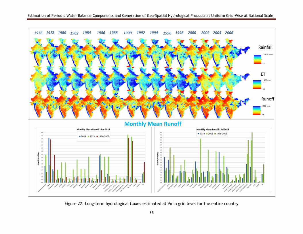
Estimation of Periodic Water Balance Components and Generation of Geo-Spatial Hydrological Products at Uniform Grid-Wise at National Scale
35
Figure 22: Long-term hydrological fluxes estimated at 9min grid level for the entire country
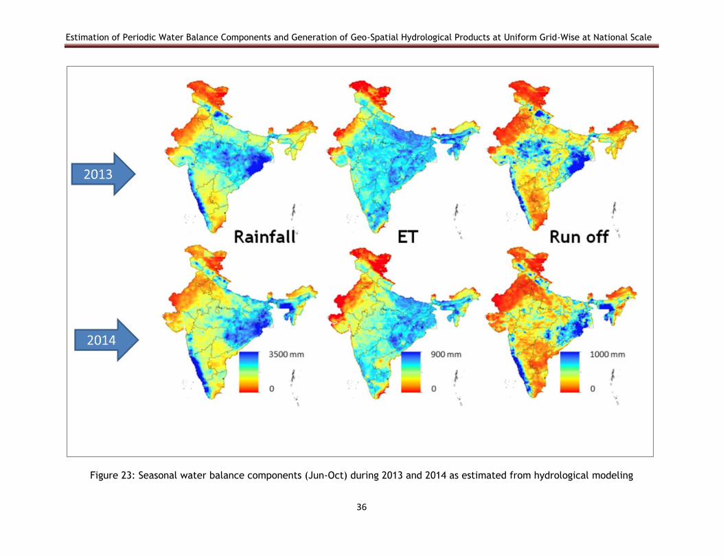
Estimation of Periodic Water Balance Components and Generation of Geo-Spatial Hydrological Products at Uniform Grid-Wise at National Scale
36
Figure 23: Seasonal water balance components (Jun-Oct) during 2013 and 2014 as estimated from hydrological modeling

Estimation of Periodic Water Balance Components and Generation of Geo-Spatial Hydrological Products at Uniform Grid-Wise at National Scale
37
Figure 24: Daily water balance components published on Bhuvan web portal
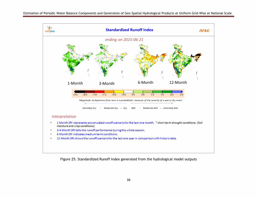
Estimation of Periodic Water Balance Components and Generation of Geo-Spatial Hydrological Products at Uniform Grid-Wise at National Scale
38
Figure 25: Standardized Runoff Index generated from the hydrological model outputs
Estimation of Periodic Water Balance Components and Generation of Geo-Spatial Hydrological Products
at Uniform Grid-Wise at National Scale
39
7. 3 minute Hydrological modeling setup
Hydrological modeling (Variable Infiltration Capacity Model) framework has been setup
at 3min (~5.5km) grid level for the Godavari, Mahanadi, Mahi and Lower Ganga basins.
Model specific input parameters (Soil, Vegetation, Routing) are prepared for the above
basins
Historical meteorological data has been organized (2001-2013) from various sources
and VIC model specific meteorological inputs are prepared
The model performance has been optimized through calibration of model estimated
runoff with measured stream discharge (CWC) using historic gridded meteorological
products from IMD (2001-2013) for selected river basins.
Long-term (1976-2013) hydrological fluxes (Surface runoff, Evapotranspiration and Soil
moisture) have been generated at 3min grid level for the Godavari and Mahanadi river
basins (Figures 25 & 26)

Estimation of Periodic Water Balance Components and Generation of Geo-Spatial Hydrological Products
at Uniform Grid-Wise at National Scale
40
2000
2005
2010
Seasonal Evapotranspiration (Jun-Oct) at 3min grid level over Godavari river basin
Seasonal Evapotranspiration (Jun-Oct) at 3min grid level over Mahanadi river basin
Figure 26: 3min Grid level water balance components

Estimation of Periodic Water Balance Components and Generation of Geo-Spatial Hydrological Products
at Uniform Grid-Wise at National Scale
41
Figure 27: Hydrological model (3min) derivatives for Mahanadi river basin
Estimation of Periodic Water Balance Components and Generation of Geo-Spatial Hydrological Products
at Uniform Grid-Wise at National Scale
42
8 FURTHER/ONGOING WORK
To operationalize Web-enabled National level hydrological modeling for in season
hydrological water balance components for the entire country at 3min grid level
To incorporate in-season satellite data based vegetation/crop information for
computing near-real-time fluxes
To estimate interventional river discharge using reservoir storage information under
WBIS
To develop and establish a comprehensive field experimentation setup for calibration
and validation of Soil Moisture, ET
Operationalization of hydrological fluxes forecasting using IMD & SAC (WRF) forecast
product
Operationalization of early warning systems (Current season deviations/extremes)
Estimation of Periodic Water Balance Components and Generation of Geo-Spatial Hydrological Products
at Uniform Grid-Wise at National Scale
43
References
1. Variable Infiltration Capacity (VIC) Macroscale Hydrologic Model, University of Washington, accessed on 13 June 2013, <http://www.hydro.washington.edu/Lettenmaier/Models/VIC/Overview/Model Overview.html >.
2. Dadhwal VK, SP Aggarwal, Nidhi Mishra (2010), ‘Hydrological Simulation of Mahanadi River Basin and Impact of land use / land cover change on surface runoff using a macro scale hydrological model’ - ISPRS Archives– Volume XXXVIII - Part 7B, ISPRS Technical Commission VII Symposium.
3. Hurkmans, R. T. W. L., De Moel, H., Aerts, J. C. J. H., and Troch, P. A. (2008). ‘Water balance versus land surface model in the simulation of Rhine river discharges’. Water Resources Research, 44(1).
4. Jha, M. K. (2011). ‘Evaluating hydrologic response of an agricultural watershed for watershed analyses. Water, 3(2), 604-617.
5. Lettenmaier D.P (2001), ‘Macroscale Hydrology: Challenges and Opportunities’ Present and Future of Modeling Global Environmental Change: Toward Integrated Modeling, pp. 111–136.
6. Liang, X., Lettenmaier, D. P., Wood, E. F. and Burges, S. J., (1994), ‘A simple hydrologically based model of land surface water and energy fluxes for general circulation models’, J. Geophys. Res., 99, 14415–14428.
7. Lohmann, D., et al. (1996), A large scale horizontal routing model to be coupled to land surface parameterization schemes, Tellus (48A), 708-721.
8. Lohmann, D., E. Raschke, B. Nijssen, and D. P. Lettenmaier (1998a), Regional scale hydrology, Part II: Application of the VIC-2L model to the Weser River, Germany, Hydrol. Sci. J., 43(1), 143–158.
9. Lohmann, D., et al. (1998b), The Project for Intercomparison of Land-Surface Parameterization Schemes (PILPS) Phase-2(c) Red-Arkansas River Basin Experiment: 3. Spatial and temporal analysis of water fluxes, J. Global Planet. Change, 19, 161–179.
10. Moriasi, D. N., Arnold, J. G., Van Liew, M. W., Bingner, R. L., Harmel, R. D., and Veith, T. L. 2007.Model evaluation guidelines for systematic quantification of accuracy in watershed simulations. Trans. ASABE, 50(3), 885-900.
11. Roy C. Ward, Robinson Mark (2000), ‘Principles of Hydrology’ McGraw-Hill 2000.
12. Suoquan Zhou, Xu Liang, Jing Chen and Peng Gong (2004), ‘An Assessment of the VIC- 3L Hydrological Model for the Baohe River Basin on RS’, Can. J. Remote Sensing, Vol. 30,No.5, pp.840–853.
13. Ven Te Chow, David R. Maidment and Larry W. Mays (1988), ‘Applied Hydrology’, pp 3-4.

Estimation of Periodic Water Balance Components and Generation of Geo-Spatial Hydrological Products
at Uniform Grid-Wise at National Scale
44
14. Xie, Z., Yuan, F., Duan, Q., Zheng, J., Liang, M., and Chen, F. (2007). Regional Parameter Estimation of the VIC Land Surface Model: Methodology and Application to River Basins in China. Journal of Hydrometeorology, 8(3).
15. Zhao, RJ., Zhuang, Y.L., Fang, L.R., Liu, X.R. and Zhang, Q.S., (1980). The Xinanjiang model. In: Hydrological Forecasting, Proceedings of the Oxford Symposium, April 1980. IAHS Publ. No. 129.
16. Laiolo. P et.al, 2016, Impact of different soil moisture products on predictions of a continuous distributed hydrological model, International Journal of Applied Earth Observation and Geo Information, 48, 131-145
17. Nash, J.E., Sutcliffe, J.V., 1970. River flow forecasting through conceptual models.
Part 1: A discussion of principles. Journal of Hydrology, 10, 282–290. 18. Todini E., 1996, The ARNO rainfall-runoff model, Journal of Hydrology, 175, 339-382 19. Zhao J., Y.-L. Zhang, L.-R. Fang, X.-R. Liu, Q.-S. Zhang, The Xinanjiang Model,
Hydrological Forecasting Proceedings Oxford Symposium, IASH, 129 (1980), pp. 351–356
20. Zhao, R., 1992. The Xinanjiang model applied in China. J. Hydrol. 135, 371 – 381

Estimation of Periodic Water Balance Components and Generation of Geo-Spatial Hydrological Products
at Uniform Grid-Wise at National Scale
45
Annexure 1
Early Warning of High Surface/River Runoff –
Hudhud Cyclone

Estimation of Periodic Water Balance Components and Generation of Geo-Spatial Hydrological Products
at Uniform Grid-Wise at National Scale
46
Experimental Surface and River Runoff forecast for Cyclone Hudhud in Catchment
areas of Nagavali and Vamsadhara rivers
As part of Operational Hydrological Products & Services, surface runoff conditions are
predicted for next three days across the country using weather forecast data. Currently, NRSC
uses NOAA Global Ensemble Forecast System Reforecast (GEFS/R) data, which provides
weather forecast for next 8 days (3hr/6hr time-step) at 0.5deg resolution
(ftp://ftp.cdc.noaa.gov/Projects/Reforecast2).
Surface Runoff Forecast
After tracking and assimilating the information on Hudhud cyclone as early as 08th Oct, 2014,
using GEFS/R weather forecast data daily surface runoff was forecasted over AP and Orissa
coast, where Cyclone was predicted to make landfall. The forecasted surface runoff
conditions were hosted on Bhuvan web portal (Figure 1).
Figure 1: Bhuvan portal depicting the surface runoff forecast on 12 Oct, 2014 for Cyclone
Hudhud using GEFS/R weather forecast data of 09 Oct, 2014
Using daily weather forecast from GEFS/R, the surface runoff forecast updated on daily basis
(Figure 2).

Estimation of Periodic Water Balance Components and Generation of Geo-Spatial Hydrological Products
at Uniform Grid-Wise at National Scale
47
08th Oct, 2014 Forecast
09th Oct, 2014 Forecast
10th Oct, 2014 Forecast
11th Oct, 2014 Forecast
0500hrs 12th Oct, 2014 Forecast
Figure 2: Daily Surface runoff forecast for Hudhud Cyclone using GEFS/R weather forecast
(Note: Date of forecast denotes the GEFS(R) forecast generation date)
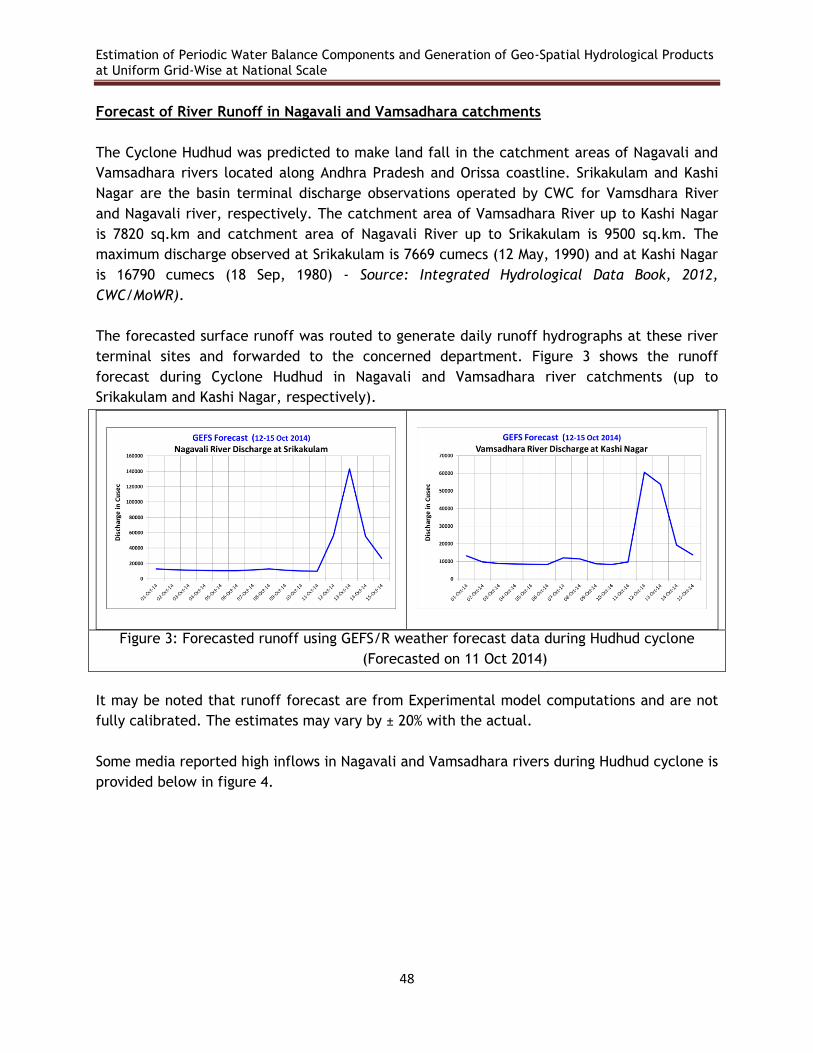
Estimation of Periodic Water Balance Components and Generation of Geo-Spatial Hydrological Products
at Uniform Grid-Wise at National Scale
48
Forecast of River Runoff in Nagavali and Vamsadhara catchments
The Cyclone Hudhud was predicted to make land fall in the catchment areas of Nagavali and
Vamsadhara rivers located along Andhra Pradesh and Orissa coastline. Srikakulam and Kashi
Nagar are the basin terminal discharge observations operated by CWC for Vamsdhara River
and Nagavali river, respectively. The catchment area of Vamsadhara River up to Kashi Nagar
is 7820 sq.km and catchment area of Nagavali River up to Srikakulam is 9500 sq.km. The
maximum discharge observed at Srikakulam is 7669 cumecs (12 May, 1990) and at Kashi Nagar
is 16790 cumecs (18 Sep, 1980) - Source: Integrated Hydrological Data Book, 2012,
CWC/MoWR).
The forecasted surface runoff was routed to generate daily runoff hydrographs at these river
terminal sites and forwarded to the concerned department. Figure 3 shows the runoff
forecast during Cyclone Hudhud in Nagavali and Vamsadhara river catchments (up to
Srikakulam and Kashi Nagar, respectively).
Figure 3: Forecasted runoff using GEFS/R weather forecast data during Hudhud cyclone
(Forecasted on 11 Oct 2014)
It may be noted that runoff forecast are from Experimental model computations and are not
fully calibrated. The estimates may vary by ± 20% with the actual.
Some media reported high inflows in Nagavali and Vamsadhara rivers during Hudhud cyclone is
provided below in figure 4.

Estimation of Periodic Water Balance Components and Generation of Geo-Spatial Hydrological Products
at Uniform Grid-Wise at National Scale
49
Figure 4: Media report depicting high runoff inflow in Nagavali and Vamsadhara river
during Hudhud cyclone.
Estimation of Periodic Water Balance Components and Generation of Geo-Spatial Hydrological Products
at Uniform Grid-Wise at National Scale
50
Annexure 2
Retrospective Analysis of Kashmir Floods

Estimation of Periodic Water Balance Components and Generation of Geo-Spatial Hydrological Products
at Uniform Grid-Wise at National Scale
51
Figure 5: Daily Runoff Estimated along Jhelum River during Kashmir flood and
comparison with historical conditions
Related Documents