ETH Library Estimation of Parameter Sensitivities for Stochastic Reaction Networks Using Tau- Leap Simulations Journal Article Author(s): Gupta, Ankit; Rathinam, Muruhan; Khammash, Mustafa Hani Publication date: 2018 Permanent link: https://doi.org/10.3929/ethz-b-000265134 Rights / license: In Copyright - Non-Commercial Use Permitted Originally published in: SIAM Journal on Numerical Analysis 56(2), https://doi.org/10.1137/17M1119445 This page was generated automatically upon download from the ETH Zurich Research Collection . For more information, please consult the Terms of use .

Welcome message from author
This document is posted to help you gain knowledge. Please leave a comment to let me know what you think about it! Share it to your friends and learn new things together.
Transcript
ETH Library
Estimation of ParameterSensitivities for StochasticReaction Networks Using Tau-Leap Simulations
Journal Article
Author(s):Gupta, Ankit; Rathinam, Muruhan; Khammash, Mustafa Hani
Publication date:2018
Permanent link:https://doi.org/10.3929/ethz-b-000265134
Rights / license:In Copyright - Non-Commercial Use Permitted
Originally published in:SIAM Journal on Numerical Analysis 56(2), https://doi.org/10.1137/17M1119445
This page was generated automatically upon download from the ETH Zurich Research Collection.For more information, please consult the Terms of use.
SIAM J. NUMER. ANAL. c\bigcirc 2018 Ankit Gupta, Muruhan Rathinam, and Mustafa KhammashVol. 56, No. 2, pp. 1134--1167
ESTIMATION OF PARAMETER SENSITIVITIES FOR STOCHASTICREACTION NETWORKS USING TAU-LEAP SIMULATIONS\ast
ANKIT GUPTA\dagger , MURUHAN RATHINAM\ddagger , AND MUSTAFA KHAMMASH\dagger
Abstract. We consider the important problem of estimating parameter sensitivities for stochas-tic models of reaction networks that describe the dynamics as a continuous time Markov process overa discrete lattice. These sensitivity values are useful for understanding network properties, validatingtheir design, and identifying the pivotal model parameters. Many methods for sensitivity estimationhave been developed, but their computational feasibility suffers from the critical bottleneck of re-quiring time-consuming Monte Carlo simulations of the exact reaction dynamics. To circumvent thisproblem, one needs to devise methods that speed up the computations while suffering acceptableand quantifiable loss of accuracy. We develop such a method by first deriving a novel integral repre-sentation of parameter sensitivity and then demonstrating that this integral may be approximatedby any convergent tau-leap method. Our method is easy to implement and works with any tau-leapsimulation scheme, and its accuracy is proved to be similar to that of the underlying tau-leap scheme.We demonstrate the efficiency of our methods through numerical examples. We also compare ourmethod with the tau-leap versions of certain finite difference schemes that are commonly used forsensitivity estimations.
Key words. parameter sensitivity, reaction networks, Markov process, tau-leap simulations
AMS subject classifications. 60J22, 60J27, 60H35, 65C05
DOI. 10.1137/17M1119445
1. Introduction. The study of chemical reaction networks is an essential com-ponent of the emerging fields of systems and synthetic biology [1, 43, 17]. Traditionallychemical reaction networks were modeled in the deterministic setting, where the dy-namics is represented by a set of ODEs or PDEs. In the study of intracellular chemicalreactions, some chemical species are present in low copy numbers. Since the behaviorof individual molecules is best described by a stochastic process, in the low molecularcopy number regime, the copy numbers of the molecular species itself are better mod-eled by a stochastic process than by ODEs [19]. Only in the limit of large molecularcopy numbers, one expects the deterministic models to be accurate [3]. While ourwork in this paper is focused on biochemical reaction networks as primary examples,we emphasize that the mathematical framework of reaction networks can also be usedto describe a wide range of other phenomena in fields such as epidemiology [27] andecology [8].
Suppose \theta is a parameter (like ambient temperature, cell volume, ATP concen-tration, etc.) that influences the rate of firing of reactions. Let (X\theta (t))t\geq 0 be the\theta -dependent Markov process representing the reaction dynamics, and suppose thatfor some real-valued function f and observation time T , our output of interest isf(X\theta (T )). This output is a random variable, and we are interested in determin-ing the sensitivity of its expectation \BbbE (f(X\theta (T ))) w.r.t. infinitesimal changes in theparameter \theta . We define this sensitivity value, denoted by S\theta (f, T ), as the partial
\ast Received by the editors March 3, 2017; accepted for publication (in revised form) February 13,2018; published electronically April 24, 2018.
http://www.siam.org/journals/sinum/56-2/M111944.html\dagger Department of Biosystems Science and Engineering, ETH Zurich, 4058 Basel, Switzerland
([email protected], [email protected]).\ddagger Department of Mathematics and Statistics, University of Maryland Baltimore County, Baltimore,
MD 21250 ([email protected]).
1134
c\bigcirc 2018 Ankit Gupta, Muruhan Rathinam, and Mustafa Khammash
Dow
nloa
ded
03/0
8/19
to 1
29.1
32.1
80.6
1. R
edis
trib
utio
n su
bjec
t to
SIA
M li
cens
e or
cop
yrig
ht; s
ee h
ttp://
ww
w.s
iam
.org
/jour
nals
/ojs
a.ph
p

SENSITIVITY ESTIMATION USING TAU-LEAP SIMULATIONS 1135
derivative
S\theta (f, T ) :=\partial
\partial \theta \BbbE (f(X\theta (T ))).(1)
Determining these parametric-sensitivity values are useful in many applications, suchas understanding network design and its robustness properties [41], identifying criticalreaction components, inferring model parameters [16], and fine-tuning a system'sbehavior [15].
Generally, the sensitivities of the form (1) cannot be directly evaluated, but in-stead, they need to be estimated with Monte Carlo simulations of the dynamics(X\theta (t))t\geq 0. Many methods have been developed for this task [23, 32, 39, 40, 2, 25, 26],but they all rely on exact simulations of (X\theta (t))t\geq 0 that can be performed usingschemes such as Gillespie's stochastic simulation algorithm (SSA) [19]. This severelyconstrains the computational feasibility of these sensitivity estimation methods be-cause these exact simulations become highly impractical if the rate of occurrence ofreactions is high [21], which is typically the case. The main difficulty is that that exactsimulation schemes keep track of each reaction event, which is very time consuming.To avoid this problem, tau-leaping methods have been developed that proceed by com-bining many reaction-firings over small time intervals [20]. Tau-leap methods havebeen shown to produce good approximations of the reaction dynamics, at a small frac-tion of the computational cost of exact simulations [20, 11, 35, 42, 5, 38, 46, 47, 28, 31].Their accuracy and stability have also been investigated theoretically in many papers[37, 30, 6, 34, 36].
Our goal in this paper is to develop a method that takes advantage of the compu-tational efficiency of tau-leap methods for the purpose of estimating sensitivity valuesof the form (1). Since tau-leap methods introduce a bias in the estimation, it is highlydesirable to start with an unbiased method for computing sensitivities (instead of bi-ased methods such as finite difference) and then replace exact SSA simulations by asuitable tau-leap method. Having only one form of bias, modulated by the tau-leapstep size, allows one to control the bias more effectively and also facilitates the designof multilevel strategies that eliminate or reduce the estimator bias and enhance itscomputational efficiency [7, 29, 31]. Among the existing methods in the literature,only the Girsanov transformation (GT) method [22, 32], the auxiliary path algorithm(APA) [25], and the Poisson path algorithm (PPA) [26] are unbiased. Since the GTmethod in general suffers from large variance [26, 2, 25, 39, 40, 44] and the APA/PPAmethods are not directly amenable to tau-leap approximation, we develop a variant ofthe PPA method in which exact SSA simulations are replaced by tau-leap simulations.Our method, called the tau integral path algorithm (\tau IPA), works with any under-lying tau-leap simulation scheme and it is based on a novel integral representationof parameter sensitivity S\theta (f, T ) that we derive in this paper. We provide computa-tional examples that show that using \tau IPA, we can often trade off a small amountof bias for large savings in the overall computational costs for sensitivity estimation.We prove that the bias incurred by \tau IPA depends on the step size in the same wayas the bias of the tau-leap scheme chosen for simulations. Moreover, if we substitutethe tau-leap simulations in \tau IPA with the exact SSA-generated simulations, then weobtain a new unbiased method for sensitivity estimation which we call the ``exact""IPA (eIPA), which is similar to the PPA method in [26]. Two main reasons for thehigh variance of the GT method that have been identified in the existing literature are(1) low magnitude of the sensitivity parameter \theta (see [26, 25]) and (2) large systemsize or volume under the classical volume scaling of the reaction network [44]. The
c\bigcirc 2018 Ankit Gupta, Muruhan Rathinam, and Mustafa Khammash
Dow
nloa
ded
03/0
8/19
to 1
29.1
32.1
80.6
1. R
edis
trib
utio
n su
bjec
t to
SIA
M li
cens
e or
cop
yrig
ht; s
ee h
ttp://
ww
w.s
iam
.org
/jour
nals
/ojs
a.ph
p
1136 A. GUPTA, M. RATHINAM, AND M. KHAMMASH
second issue is somewhat resolved by the centered Girsanov transformation (CGT)method [44, 51], and our numerical results indicate that the volume scaling behav-ior of eIPA is similar to CGT (see section 4.1). However, eIPA does not suffer fromhigh variance when the sensitivity parameter \theta is small. In addition, when \theta = 0,GT or CGT methods are not even applicable, while eIPA does not suffer from thisrestriction. These observations make eIPA more appealing than CGT for unbiasedestimation of parameter sensitivity.
For the sake of comparison, we use tau-leap versions of certain commonly usedfinite difference estimators (see [2, 39, 50]) that approximate the infinitesimal deriva-tive in (1) by a finite difference (see (11)). Such estimators are computationally fasterthan \tau IPA (in simulation time per trajectory), but they suffer from two sources of bias(finite differencing and tau-leap approximations) unlike \tau IPA, which only incurs biasfrom the latter source. We note that while in some examples the biases nearly canceleach other fortuitously, as a general principle one has no logical reason to expect suchcancellation.
This paper is organized as follows. In section 2 we describe the stochastic modelfor reaction dynamics and the sensitivity estimation problem. We also discuss the ex-isting sensitivity estimation methods and the tau-leap simulation schemes and explainthe rationale for using such simulations in sensitivity estimation. Section 3 containsthe main results of this paper, which include a novel integral representation of theexact sensitivity in section 3.2, a result on error bounds for the sensitivity estimatesof \tau IPA in section 3.3, and a novel tau-leap sensitivity estimation method, \tau IPA, insection 3.4. In section 4 we provide computational examples to compare our methodwith other methods, and finally in section 5 we conclude and provide directions forfuture research.
2. Preliminaries. Consider a reaction network with d species and K reactions.We describe its kinetics by a continuous time Markov process whose state at any timeis a vector in the nonnegative integer orthant \BbbN d
0 comprising the molecular counts ofall the d species. The state evolves due to transitions caused by the firing of reactions.We suppose that when the state is x, the rate of firing of the kth reaction is given bythe propensity function \lambda k(x) and the corresponding state-displacement is denoted bythe stoichiometric vector \zeta k \in \BbbZ d. There are several ways to represent the Markovprocess (X(t))t\geq 0 that describes the reaction kinetics under these assumptions. Wecan specify the generator (see Chapter 4 in [14]) of this process by the operator
\BbbA h(x) =K\sum
k=1
\lambda k(x) (h(x+ \zeta k) - h(x)) ,(2)
where h is any bounded real-valued function on \BbbN d0. Alternatively, we can express
the Markov process directly by its random time-change representation (see Chapter 7in [14]),
X(t) = X(0) +
K\sum k=1
Yk
\biggl( \int t
0
\lambda k(X(s))ds
\biggr) \zeta k,(3)
where \{ Yk : k = 1, . . . ,K\} is a family of independent unit rate Poisson processes. Sincethe process (X(t))t\geq 0 is Markovian, it can be equivalently specified by writing theKolmogorov forward equation for the evolution of its probability distribution pt(x) :=\BbbP (X(t) = x) at each state x:
c\bigcirc 2018 Ankit Gupta, Muruhan Rathinam, and Mustafa Khammash
Dow
nloa
ded
03/0
8/19
to 1
29.1
32.1
80.6
1. R
edis
trib
utio
n su
bjec
t to
SIA
M li
cens
e or
cop
yrig
ht; s
ee h
ttp://
ww
w.s
iam
.org
/jour
nals
/ojs
a.ph
p

SENSITIVITY ESTIMATION USING TAU-LEAP SIMULATIONS 1137
dpt(x)
dt=
K\sum k=1
pt(x - \zeta k)\lambda k(y - \zeta k) - pt(x)
K\sum k=1
\lambda k(x).(4)
This set of coupled ODEs is termed the chemical master equation (CME) in thebiological literature [3]. As the number of ODEs in this set is typically infinite,the CME is nearly impossible to solve directly, except in very restrictive cases. Acommon strategy is to estimate its solution using pathwise simulations of the process(X(t))t\geq 0 using Monte Carlo schemes such as Gillespie's SSA [19], the next reactionmethod [18], the modified next reaction method [4], and so on. While these schemesare easy to implement, they become computationally infeasible for even moderatelylarge networks because they account for each and every reaction event. To resolve thisissue, tau-leaping methods have been developed, which will be described, in greaterdetail in section 3.1.
We now assume that each propensity function \lambda k depends on a real-valued systemparameter \theta . To emphasize this dependence, we write the rate of firing of the kthreaction at state x as \lambda k(x, \theta ) instead of \lambda k(x). Let (X\theta (t))t\geq 0 be the Markov pro-cess representing the reaction dynamics with these parameter-dependent propensityfunctions. As stated in the introduction, for a function f : \BbbN d
0 \rightarrow \BbbR and an obser-vation time T \geq 0, our goal is to determine the sensitivity value S\theta (f, T ) defined by(1). This value cannot be computed directly for most examples of interest, and so weneed to find ways of estimating it using simulations of the process (X\theta (t))t\geq 0. Suchsimulation-based sensitivity estimation methods work by specifying the constructionof a random variable s\theta (f, T ) whose expected value is ``close"" to the true sensitivityvalue S\theta (f, T ), i.e.,
S\theta (f, T ) \approx \BbbE (s\theta (f, T )).(5)
Once such a construction is available, a large number (say N) of independent realiza-tions s1, . . . , sN of this random variable s\theta (f, T ) are obtained, and the sensitivity isestimated by computing their empirical mean \^\mu N as
\^\mu N =1
N
N\sum i=1
si.(6)
This estimator \^\mu N is a random variable with mean and variance
\mu = \BbbE (\^\mu N ) = \BbbE (s\theta (f, T )) and \sigma 2N = Var(\^\mu N ) =
\sigma 2
N,(7)
respectively, where \sigma 2 = Var(s\theta (f, T )). For a large sample size N , the distribution of\^\mu N is approximately Gaussian with mean \mu and variance \sigma 2
N due to the central limittheorem. The standard deviation \sigma N measures the statistical spread of the estimator\^\mu N that is inversely proportional to its statistical precision. The sample size N mustbe large enough to ensure that \sigma N is small relative to \mu ; i.e., for some small parameter\epsilon > 0, we should have
RSD\surd N\leq \epsilon ,(8)
where RSD := \sigma /| \mu | is the relative standard deviation of the random variable s\theta (f, T ).If such a condition holds, then \^\mu N is a reliable estimator for the true sensitivity value
c\bigcirc 2018 Ankit Gupta, Muruhan Rathinam, and Mustafa Khammash
Dow
nloa
ded
03/0
8/19
to 1
29.1
32.1
80.6
1. R
edis
trib
utio
n su
bjec
t to
SIA
M li
cens
e or
cop
yrig
ht; s
ee h
ttp://
ww
w.s
iam
.org
/jour
nals
/ojs
a.ph
p
1138 A. GUPTA, M. RATHINAM, AND M. KHAMMASH
S\theta (f, T ) because it is very likely to assume a value close to its mean \mu = \BbbE (s\theta (f, T )),which in turn is close to S\theta (f, T ) (see (5)). In practice, both \mu and \sigma are unknown,but we can estimate them as \mu \approx \^\mu N and \sigma \approx
\surd N \^\sigma N , where
\^\sigma N =1\sqrt{}
N(N - 1)
\sqrt{} N\sum i=1
(si - \^\mu N )2(9)
is the estimated standard deviation \sigma N of the estimator.The performance of any sensitivity estimation method (say \scrX ) depends on the fol-
lowing three key metrics that are based on the properties of random variable s\theta (f, T ):1. The bias \scrB (\scrX ) = \BbbE (s\theta (f, T )) - S\theta (f, T ), which is the error incurred by the
approximation (5).2. The variance \scrV (\scrX ) = Var(s\theta (f, T )) of random variable s\theta (f, T ).3. The computational cost \scrC (\scrX ) of generating one sample of s\theta (f, T ).
The bias \scrB (\scrX ) can be positive or negative, and its absolute value | \scrB (\scrX )| can be seenas the upper bound on the statistical accuracy that can be achieved with method\scrX by increasing the sample size N [9]. As mentioned before, the standard deviation\sigma (\scrX ) =
\sqrt{} \scrV (\scrX ) measures the statistical precision of the method \scrX , and its magnitude
relative to the mean \mu (\scrX ) = \BbbE (s\theta (f, T )) determines the number of samples N thatis needed to produce a reliable estimate. In particular, to satisfy condition (8) forthe relative standard deviation RSD(\scrX ) = \sigma (\scrX )/| \mu (\scrX )| , the number of samples N\epsilon
needed would be around N\epsilon := (RSD(\scrX ))2\epsilon - 2. Hence, the total cost of the estimationprocedure is
N\epsilon \scrC (\scrX ) \approx (RSD(\scrX ))2\scrC (\scrX )\epsilon - 2 =\scrV (\scrX )
(\mu (\scrX ))2\scrC (\scrX )\epsilon - 2,(10)
where \scrC (\scrX ) is the CPU time required for constructing one realization of s\theta (f, T ). Thegoal of a good estimation method is to simultaneously minimize the three quantities| \scrB (\scrX )| , \scrV (\scrX ), and \scrC (\scrX ). This creates various conflicts and trade-offs among theexisting sensitivity estimation methods as we now discuss.
2.1. Biased methods. A sensitivity estimation method \scrX is called biased if\scrB (\scrX ) \not = 0. The most commonly used biased methods are the finite difference schemeswhich approximate the infinitesimal derivative in the definition of parameter sensitiv-ity (see (1)) by a finite difference of the form
S\theta ,h(f, T ) =\BbbE (f(X\theta +h(T )) - f(X\theta (T )))
h(11)
for a small perturbation h. The processes X\theta and X\theta +h represent the Markovian re-action dynamics with values of the sensitive parameter set to \theta and \theta +h, respectively.These two processes can be simulated independently [23] but it is generally better tocouple them in order to reduce the variance of the associated estimator. The twocommonly used coupling strategies are called common reaction paths (CRP) [39] andcoupled finite differences (CFD) [2], and they are based on the random time-changerepresentation (3).
The finite difference approximation (11) for the true sensitivity value can beexpressed as the expectation \BbbE (s\theta ,h(f, T )) of the following random variable:
s\theta ,h(f, T ) =f(X\theta +h(T )) - f(X\theta (T ))
h.
c\bigcirc 2018 Ankit Gupta, Muruhan Rathinam, and Mustafa Khammash
Dow
nloa
ded
03/0
8/19
to 1
29.1
32.1
80.6
1. R
edis
trib
utio
n su
bjec
t to
SIA
M li
cens
e or
cop
yrig
ht; s
ee h
ttp://
ww
w.s
iam
.org
/jour
nals
/ojs
a.ph
p
SENSITIVITY ESTIMATION USING TAU-LEAP SIMULATIONS 1139
The three metrics (bias, variance, and computational cost) based on this randomvariable define the performance of CRP and CFD. Since both these methods estimatethe same quantity S\theta ,h(f, T ), they have the same bias (i.e., \scrB (CRP) = \scrB (CFD)).However, in many cases it is found that the CFD coupling is tighter than the CRPcoupling, resulting in a lower variance of s\theta ,h(f, T ) (i.e., \scrV (CFD) < \scrV (CRP)) (see[2]). For each realization of s\theta ,h(f, T ), both CRP and CFD require simulation of acoupled trajectory (X\theta , X\theta +h) in the time interval [0, T ]. The computational costs ofsuch a simulation is roughly 2\scrC 0, where \scrC 0 is the cost of exactly simulating the processX\theta using Gillespie's SSA [19] or a similar method.1
Finite difference schemes introduce a bias in the estimate whose size is propor-tional to the perturbation value h (i.e., \scrB (CRP) = \scrB (CFD) \propto h), but the constantof proportionality can be quite large in many cases, leading to significant errorseven for small values of h [26]. Unfortunately, we cannot circumvent this prob-lem by choosing a very small h because the variance is proportional to 1/h (i.e.,\scrV (CRP),\scrV (CFD) \propto 1/h). Therefore, if a very small h is selected, the variance will beenormous, and the sample size required to produce a statistically precise estimate willbe very large, imposing a heavy computational burden on the estimation procedure[26]. This trade-off between bias and variance is the main drawback of finite differenceschemes, and there does not exist a strategy for selecting h that optimally balancesthese two quantities. Note that unlike bias and variance, the computational cost ofgenerating a sample (i.e., \scrC (CRP) or \scrC (CFD)) does not change significantly with h,thereby ensuring that regardless of h, the total computational burden varies linearlywith the required number of samples N . Apart from finite difference schemes, thereexists another biased method, called the regularized pathwise-derivative method [40],for estimating the sensitivity value (1), but we do not discuss this approach in thispaper.
2.2. Unbiased methods. A sensitivity estimation method \scrX is called unbiasedif \scrB (\scrX ) = 0. The main advantage of unbiased methods is that the estimation can inprinciple be made as accurate as possible by increasing the sample size N . The firstunbiased method for sensitivity estimation is the GT method [22, 32], which works byestimating the \theta -derivative of the probability distribution of X\theta . The GT method iseasy to implement, and the computation cost of generating each sample is roughly \scrC 0---the cost of exact simulation of the process X\theta . The main issue with the GT methodis that generally the variance of its associated random variable s\theta (f, T ) is very large,and so the number of samples needed to obtain a statistically precise estimate is veryhigh [2, 39]. So far, two reasons have been identified for this behavior. First, it hasbeen shown that for mass-action models (see [3]), this variance can become unboundedwhen the magnitude of the sensitive reaction rate constant \theta approaches zero [26, 25].This is a serious issue because biological networks often consist of slow reactions,which are characterized by low values of the associated rate constants. Furthermore,the GT method does not allow one to estimate the sensitivity w.r.t. a rate constantset to zero. Such sensitivity values are useful for understanding network design, asit allows one to probe the effect of presence or absence of reactions. Another reasonfor the high variance of GT estimator was provided in [44], where it was theoreticallyestablished that this variance can grow boundlessly as the system expands in size;
1In fact, the cost of generating a realization of s\theta (f, T ) is usually smaller for CFD in comparisonto CRP (i.e., \scrC (CFD) < \scrC (CRP)) because the CFD coupling is such that if X\theta (t) = X\theta +h(t) forsome t < T , then this equality will hold for the remaining time interval [t, T ], allowing us to directlyset s\theta ,h(f, T ) = 0 without completing the simulation in the interval [t, T ].
c\bigcirc 2018 Ankit Gupta, Muruhan Rathinam, and Mustafa Khammash
Dow
nloa
ded
03/0
8/19
to 1
29.1
32.1
80.6
1. R
edis
trib
utio
n su
bjec
t to
SIA
M li
cens
e or
cop
yrig
ht; s
ee h
ttp://
ww
w.s
iam
.org
/jour
nals
/ojs
a.ph
p

1140 A. GUPTA, M. RATHINAM, AND M. KHAMMASH
Table 1Trade-off relationships among the bias \scrB (\scrX ), variance \scrV (\scrX ), and the computational cost \scrC (\scrX )
for existing sensitivity estimation methods. Here h is the perturbation size for finite differenceschemes [2, 39], and M0 quantifies the number of auxiliary paths for APA [25] and PPA [26]. Thecost of exactly simulating the underlying process is \scrC 0.
Type Method Trade-off Trade-off Preserved\scrX quantities parameter quantity
BiasedCRP \scrB (\scrX ) \& \scrV (\scrX ) h \scrC (\scrX ) \approx 2\scrC 0CFD
UnbiasedAPA \scrV (\scrX ) \& \scrC (\scrX ) M0 \scrB (\scrX ) = 0PPA
i.e., the system volume V tends to infinity. This issue is somewhat ameliorated bythe CGT method [51], but the problem with small reaction rate constants persists.
We now discuss a couple of unbiased methods that have been recently proposed.These methods are the APA [25] and the PPA [26], and they are based on exact rep-resentations of the form (5) for the parameter sensitivity (1). For both the methods,sampling the random variable s\theta (f, T ) requires simulation of a fixed number M0 ofadditional paths of the process X\theta . It was shown in [25] that in comparison to the GTmethod, the computational cost of generating each sample for APA is much higher(i.e., \scrC (APA)\gg \scrC (GT)), but this is often compensated by the fact that its variance ismuch lower (i.e., \scrV (APA)\ll \scrV (GT)), resulting in a smaller overall cost of estimation(10). The reason for the higher sampling cost for APA is that it needs estimates ofcertain unknown quantities at each jump time of the process X\theta in the time inter-val [0, T ], which can be very large in number even for small networks. In PPA, thisproblem is resolved by randomly selecting a small number of these unknown quanti-ties for estimation in such a way that the estimator remains unbiased. Due to thisextra randomness, the sample variance for PPA is generally greater than APA (i.e.,\scrV (PPA) > \scrV (APA)), but the computational cost for realizing each sample is muchlower (i.e., \scrC (PPA)\ll \scrC (APA)). Moreover, in comparison to APA, PPA is far easierto implement and has lower memory requirements, making it an attractive unbiasedmethod for sensitivity estimation. In [26], it is shown using many examples that fora given level of statistical accuracy, PPA can be more efficient than GT and also thefinite difference schemes CFD and CRP. The computational cost of generating eachsample in PPA is roughly (2M0+1)\scrC 0, where M0 is a small number that upper boundsthe expected number of unknown quantities that will be estimated using additionalpaths. For both APA and PPA, the parameter M0 serves as a trade-off factor betweenthe computational cost and the variance---as M0 increases, the cost also increases butthe variance decreases. However, both these methods remain unbiased for any choiceof M0.
The foregoing trade-off relationships for the existing sensitivity estimation meth-ods are summarized in Table 1.
2.3. Rationale for using tau-leap schemes for sensitivity estimation. Allthe existing sensitivity estimation methods suffer from a critical bottleneck---they areall based on exact simulations of the process X\theta . The computational cost \scrC 0 of gen-erating each trajectory of X\theta can be exorbitant even for moderately large networkswhen those networks have some molecular species in moderately large copy numbersand/or reactions firing at multiple time scales (stiff systems). One way to counterthis problem is to develop methods that can accurately estimate parameter sensi-tivities with approximate computationally inexpensive simulations of the process X\theta
c\bigcirc 2018 Ankit Gupta, Muruhan Rathinam, and Mustafa Khammash
Dow
nloa
ded
03/0
8/19
to 1
29.1
32.1
80.6
1. R
edis
trib
utio
n su
bjec
t to
SIA
M li
cens
e or
cop
yrig
ht; s
ee h
ttp://
ww
w.s
iam
.org
/jour
nals
/ojs
a.ph
p

SENSITIVITY ESTIMATION USING TAU-LEAP SIMULATIONS 1141
obtained with tau-leap methods. The use of tau-leap simulations provides a naturalway to trade off a small amount of error with a potentially large reduction in thecomputational costs.
The explicit tau-leap method with Poisson random numbers proposed by Gillespie[20] generally works well in nonstiff situations and when molecular copy numbers aremodestly large. The major drawback is that it becomes inefficient for stiff systemswhere vastly different time scales are present. The implicit tau-leap was proposedto remedy this weakness [35]. Many other tau-leap methods and step size selectionstrategies have been proposed to address stiffness and other issues [11, 42, 5, 38, 47,46, 31].
In the context of stiff systems, tau-leap methods have not been as successfulin maintaining accuracy while reducing computational cost in comparison with thesuccess of stiff solvers for deterministic differential equations. This is because stiffnessmanifests in a more complex manner in stochastic systems where stability is not theonly issue, but accurately capturing the asymptotic distribution of the fast variablesis also important [35, 36, 48, 49]. We shall limit our attention to nonstiff or modestlystiff systems in this paper.
Our goal in this paper is to develop a method that can estimate parameter sensi-tivity S\theta (f, T ) of the form (1) using only tau-leap simulations of the process X\theta . This
can be done by specifying a random variable s(\tau )\theta (f, T ) which can be constructed with
these tau-leap simulations and whose expected value is ``close"" to the true sensitivityvalue S\theta (f, T ), i.e.,
S\theta (f, T ) \approx \BbbE (s(\tau )\theta (f, T )).(12)
We propose such a random variable s(\tau )\theta (f, T ) in this paper and provide a simple
algorithm for generating the realizations of s(\tau )\theta (f, T ). We theoretically show that un-
der certain reasonable conditions, the associated estimator is tau-convergent, whichmeans that the bias incurred due to the approximation in (12) converges to 0, as themaximum step size \tau max or the coarseness of the time-discretization mesh goes to0. Hence, by making this mesh finer and finer, we can make the estimator as accu-rate as we desire, provided that we are willing to bear the increasing computationalcosts. In the context of estimating expected values \BbbE (f(X\theta (T ))), the property oftau-convergence along with the rate of convergence has already been established formany tau-leap schemes [37, 30, 6, 34]. We use these preexisting results and obtain asimilar tau-convergence result for our sensitivity estimation method. An importantfeature of our approach is that it is completely flexible as far as the choice of thetau-leap simulation method is concerned. Furthermore, the order of accuracy of oursensitivity estimation method is the same as the order of accuracy of the underlyingtau-leap method.
We end this section with observing that incorporating tau-leap schemes in sensi-tivity estimation opens up a new dimension in attacking this challenging problem. Inthe trade-off relationships for existing sensitivity estimation methods (see Table 1),parameters like h and M0 only allow us to explore one trade-off curve between thevariance \scrV (\scrX ) and some other metric like the bias \scrB (\scrX ) (for \scrX = CRP, CFD) or thecomputational cost \scrC (\scrX ) (for \scrX = APA, PPA). The main advantage of employingtau-leap schemes is that they provide a mechanism for exploring another trade-offcurve between the bias \scrB (\scrX ) and the computational cost \scrC (\scrX ) for the purpose of op-timizing the performance of a sensitivity estimation method. In section 4, we providenumerical examples to show that with tau-leap simulations, we can indeed trade off
c\bigcirc 2018 Ankit Gupta, Muruhan Rathinam, and Mustafa Khammash
Dow
nloa
ded
03/0
8/19
to 1
29.1
32.1
80.6
1. R
edis
trib
utio
n su
bjec
t to
SIA
M li
cens
e or
cop
yrig
ht; s
ee h
ttp://
ww
w.s
iam
.org
/jour
nals
/ojs
a.ph
p

1142 A. GUPTA, M. RATHINAM, AND M. KHAMMASH
a small amount of bias with large savings in the computational effort required forestimating parameter sensitivity. Moreover, this trade-off relationship appears to beindependent of existing trade-off relationships mentioned in Table 1 because replacingexact simulations in a sensitivity estimation method, with approximate tau-leap sim-ulations, usually does not alter the variance \scrV (\scrX ) significantly, at least when the taustep size is sufficiently small (see section 4). Of course, the computational advantageof tau-leap schemes can only be appropriated if we can incorporate them into existingsensitivity estimation methods. The main contribution of this paper is to developa method, similar to PPA, that works well with tau-leap schemes (see section 3).For the sake of comparison, we also provide tau-leap versions of the finite differenceschemes (CRP and CFD) in section 4.
3. Sensitivity estimation with tau-leap simulations. In this section, wepresent our approach for accurately estimating parameter sensitivities of the form (1)with only approximate tau-leap simulations of the dynamics. This approach is basedon an exact integral representation for parameter sensitivity given in section 3.2.With this representation at hand, we construct a tau-leap estimator for parametersensitivity and examine its convergence properties as the time-discretization meshgets finer and finer (see sections 3.3 and 3.4). Thereafter, in section 3.5 we present analgorithm that computes the tau-leap estimator for sensitivity estimation. We startwith the description of a generic tau-leap method that approximately simulates thestochastic reaction paths defined by the Markov process (X(x0, t))t\geq 0 with generator\BbbA (see (2)) and initial state x0.
3.1. A generic tau-leap method. For each reaction k = 1, . . . ,K, let Rk(t)be the number of firings of reaction k until time t. Due to (3), we can express eachRk(t) as
Rk(t) = Yk
\biggl( \int t
0
\lambda k(X(x0, s))ds
\biggr) \zeta k,
where \{ Yk : k = 1, . . . ,K\} is a family of independent unit rate Poisson processes.From now on, we refer to R(t) = (R1(t), . . . , RK(t)) as the reaction count vector.For any two time values s, t \geq 0 (with s < t), the states at these times satisfy
X(x0, t) = X(x0, s)+\sum K
k=1(Rk(t) - Rk(s))\zeta k. At any given time t and the computed(approximate) state x at time t, a tau-leap method entails taking a predetermined(random) step of size \tau > 0, based on the information available at time t, and thengenerating a sample from an approximating distribution for the state at time (t+ \tau ).This distribution is generally found by approximating the difference (R(t+ \tau ) - R(t))in the reaction count vector by a random variable \~R = ( \~R1, . . . , \~RK) whose probabil-ity distribution is easy to sample from. The most straightforward choice is given bythe simple (explicit) Euler method [20], which assumes that the propensities are ap-proximately constant in the time interval [t, t+\tau ) and conditioned on the informationat time t, each \~Rk being an independent Poisson random variable with rate \lambda k(x)\tau .Other distributions for \~R = ( \~R1, . . . , \~RK) have also been used in the literature toobtain better approximations and particularly to prevent the state components frombecoming negative [42]. The selection method for step size \tau also varies, with thesimplest being steps based on a deterministic mesh 0 = t0 < t1 \cdot \cdot \cdot < tn = T overthe observation time interval [0, T ]. To obtain better accuracy, several strategies havebeen proposed that randomly select \tau based on some criteria such as avoidance ofnegative state components or constancy of conditional propensities [11, 5, 31].
c\bigcirc 2018 Ankit Gupta, Muruhan Rathinam, and Mustafa Khammash
Dow
nloa
ded
03/0
8/19
to 1
29.1
32.1
80.6
1. R
edis
trib
utio
n su
bjec
t to
SIA
M li
cens
e or
cop
yrig
ht; s
ee h
ttp://
ww
w.s
iam
.org
/jour
nals
/ojs
a.ph
p
SENSITIVITY ESTIMATION USING TAU-LEAP SIMULATIONS 1143
To represent a generic tau-leap method, we shall use a pair of abstract labels \alpha and \beta , where \alpha denotes a method, i.e., a choice of distribution for \~R, and \beta denotesa step size selection strategy. We will use | \beta | as a (deterministic) parameter whichquantifies the coarseness of the time-discretization scheme \beta . For instance, \alpha maystand for the explicit Euler tau-leap method [20], and \beta may stand for a deterministicmesh 0 = t0 < t1 < \cdot \cdot \cdot < tn = T , and in this case the coarseness parameter is| \beta | = max(tj - tj - 1). Typically, tau-leap methods produce approximations of theunderlying process at certain leap times that are separated by the step size \tau , andone can interpolate these approximate state values at other time points. The mostobvious interpolation is the ``sample and hold"" method, where the tau-leap process isheld constant between the consecutive leap times. In circumstances such as the explicitEuler tau-leap method with Poisson updates, it is more natural to use interpolationstrategies based on the random time-change representation (3)---for example, see the``Poisson bridge"" approach in [28]. In the following discussion, we suppose that theinterpolation strategy is also determined by the label \alpha . We shall use (Z\alpha ,\beta (x0, t))t\geq 0
to denote the tau-leap process that approximates the exact dynamics (X(x0, t))t\geq 0
and that results from the application of a tau-leap method \alpha with step size selectionstrategy \beta . This process is defined by the prescription Z\alpha ,\beta (x0, t0) = x0 and
(13) Z\alpha ,\beta (x0, ti+1) = Z\alpha ,\beta (x0, ti) +
K\sum k=1
\zeta k \~Rk,i,\alpha ,\beta for i = 1, . . . , \mu ,
where \mu is the (possibly) random number of time points, 0 = t0 < t1 < \cdot \cdot \cdot < t\mu = T
are the (possibly) random leap times, and \~Rk,i,\alpha ,\beta for i = 1, . . . , \mu and k = 1, . . . ,Kare random variables whose distribution when conditioned on Z\alpha ,\beta (x, ti) is determinedby the method \alpha and step size strategy \beta .
Remark 3.1. Note that this generic tau-leap method reduces to Gillespie's SSA[19] if at state Z\alpha ,\beta (x0, ti) = z, the next step size \tau is an exponentially distributed
random variable with rate \lambda 0(z) :=\sum K
k=1 \lambda k(z) and each \~Rk,i,\alpha ,\beta is chosen as 1 ifk = \eta and 0 otherwise, where \eta is a discrete random variable which assumes the valuei \in \{ 1, . . . ,K\} with probability (\lambda i(z)/\lambda 0(z)).
Later we shall establish tau-convergence of our sensitivity estimator by showingthat for a fixed tau-leap method \alpha , the bias incurred by our estimator converges to0 as the coarseness | \beta | of the time-discretization scheme goes to 0. For this, we shallrequire (weak) convergence of all moments of the tau-leap process to those of theexact process. We now state this requirement more precisely and present a simplelemma that will be needed later. For p \geq 0, we say that a function f : \BbbN d
0 \rightarrow \BbbR is ofclass \scrC p if there exists a positive constant C such that
| f(x)| \leq C(1 + \| x\| p) for all x \in \BbbN d0.(14)
We shall require that a tau-leap method \alpha satisfies an order \gamma > 0 convergent errorbound. This is stated formally by Assumption 1, and it can be verified using theresults in [34].
Assumption 1. Given a tau-leap method \alpha , there exist \gamma > 0, \delta > 0 and amapping \xi : \BbbR + \rightarrow \BbbR + such that, for every p \geq 0 and every final time T > 0, thereexists a constant C1(p, T, \alpha ) satisfying
c\bigcirc 2018 Ankit Gupta, Muruhan Rathinam, and Mustafa Khammash
Dow
nloa
ded
03/0
8/19
to 1
29.1
32.1
80.6
1. R
edis
trib
utio
n su
bjec
t to
SIA
M li
cens
e or
cop
yrig
ht; s
ee h
ttp://
ww
w.s
iam
.org
/jour
nals
/ojs
a.ph
p

1144 A. GUPTA, M. RATHINAM, AND M. KHAMMASH
supt\in [0,T ]
| \BbbE (\| Z\alpha ,\beta (x0, t)\| p) - \BbbE (\| X(x0, t)\| p)|
\leq supt\in [0,T ]
\sum y\in \BbbN d
0
(1 + \| y\| p)| \BbbP (Z\alpha ,\beta (x0, t) = y) - \BbbP (X(t, x0) = y)|
\leq C1(p, T, \alpha )(1 + \| x0\| \xi (p))| \beta | \gamma
for any initial state x0 provided that | \beta | \leq \delta . Note that here the second inequalityis our assumption while the first inequality always holds. In above, we have assumed(\Omega , P ) and (\~\Omega , \~P ) to be probability spaces that carry the exact process X and thetau-leap process Z\alpha ,\beta .
Additionally, we will require Assumptions 2 and 3 on moment growth bounds ofthe exact process as well as the tau-leap process. These assumptions can be verifiedusing the results in [33, 24, 34].
Assumptions 2 and 3. Given a tau-leap method \alpha , there exists \delta > 0 such thatfor each T > 0 and p \geq 0, there exist constants C2(p, T ) and C3(p, T, \alpha ) satisfying
supt\in [0,T ]
(1 + \BbbE (\| X(x0, t)\| p)) \leq C2(p, T )(1 + \| x0\| p)
and supt\in [0,T ]
(1 + \BbbE (\| Z\alpha ,\beta (x0, t)\| p)) \leq C3(p, T, \alpha )(1 + \| x0\| p)(15)
for all t \in [0, T ] provided | \beta | \leq \delta .We emphasize that constants C1 and C3 in Assumptions 1 and 3 do not depend
on the step size selection strategy \beta , and all the three constants in these assumptionsmay be assumed to be monotonic in T without any loss of generality. The followinglemma follows readily from the above assumptions.
Lemma 3.2. Consider a function \phi : \BbbN d0 \times [0, T ] \rightarrow \BbbR , and suppose that there
exists a constant C > 0 such that supt\in [0,T ] | \phi (x, t)| \leq C(1 + \| x\| p) for all x \in \BbbN d0.
Then under Assumptions 1, 2, and 3, we have(16)
supt\in [0,T ]
| \BbbE (\phi (Z\alpha ,\beta (x0, t), t)) - \BbbE (\phi (X(x0, t), t))| \leq CC1(p, T, \alpha )(1 + \| x0\| \xi (p))| \beta | \gamma ,
supt\in [0,T ]
| \BbbE (\phi (X(x0, t), t))| \leq CC2(p, T )(1 + \| x0\| p)
and supt\in [0,T ]
| \BbbE (\phi (Z\alpha ,\beta (x0, t), t))| \leq CC3(p, T, \alpha )(1 + \| x0\| p)
provided | \beta | \leq \delta .
3.2. An integral formula for parameter sensitivity. Let (X\theta (t))t\geq 0 be theMarkov process representing reaction dynamics with initial state x0, and let \Psi \theta (x, f, t)be defined by
\Psi \theta (x, f, t) = \BbbE (f(X\theta (t))| X\theta (0) = x)(17)
for any state x \in \BbbN d0 and time t \geq 0. For any k = 1, . . . ,K and any function
h : \BbbN d0 \rightarrow \BbbR , let \Delta \zeta k , denote the difference operator given by
\Delta \zeta kh(x) = h(x+ \zeta k) - h(x).
The following theorem expresses the sensitivity value S\theta (f, T ) as the expectation ofa random variable which can be computed from the paths of the process (X\theta (t))t\geq 0
in the time interval [0, T ]. The proof of this theorem is provided in Appendix A.
c\bigcirc 2018 Ankit Gupta, Muruhan Rathinam, and Mustafa Khammash
Dow
nloa
ded
03/0
8/19
to 1
29.1
32.1
80.6
1. R
edis
trib
utio
n su
bjec
t to
SIA
M li
cens
e or
cop
yrig
ht; s
ee h
ttp://
ww
w.s
iam
.org
/jour
nals
/ojs
a.ph
p

SENSITIVITY ESTIMATION USING TAU-LEAP SIMULATIONS 1145
Theorem 3.3. Suppose (X\theta (t))t\geq 0 is the Markov process with generator \BbbA \theta andinitial state x0. Then the sensitivity value S\theta (f, T ) is given by
S\theta (f, T ) =\partial
\partial \theta \Psi \theta (x0, f, T ) =
K\sum k=1
\BbbE
\Biggl( \int T
0
\partial \lambda k(X\theta (t), \theta )
\partial \theta \Delta \zeta k\Psi \theta (X\theta (t), f, T - t)dt
\Biggr) .
Remark 3.4. This formula has the following simple interpretation. Due to aninfinitesimal perturbation of parameter \theta , the probability that the process (X\theta (t))t\geq 0
has an ``extra"" jump at time t in the direction \zeta k is proportional to
\partial \lambda k(X\theta (t), \theta )
\partial \theta .
Moreover, the change in the expectation of f(X\theta (T )) at time T due to this ``extra""jump at time t is just
\Delta \zeta k\Psi \theta (X\theta (t) + \zeta k, f, T - t).
The above result shows that the overall sensitivity of the expectation of f(X\theta (x, T ))is just the product of these two terms, integrated over the whole time interval [0, T ].
The rest of this section is devoted to the development of a tau-leap estimatorfor parameter sensitivity using this formula. To simplify our notations, we suppressthe dependence on parameter \theta and hence denote \lambda k(\cdot , \theta ) by \lambda k(\cdot ), \partial \lambda k/\partial \theta by \partial \lambda k,S\theta (f, T ) by S(f, T ), \Psi \theta (x, f, t) by \Psi (x, f, t), and the process (X\theta (t))t\geq 0 by (X(t))t\geq 0.Due to Theorem 3.3, the sensitivity value S(f, T ) can be expressed as
S(f, T ) =
K\sum k=1
\BbbE
\Biggl( \int T
0
\partial \lambda k(X(t))\Delta \zeta k\Psi (X(t), f, T - t)dt
\Biggr) .(18)
3.3. Sensitivity approximation with tau-leap simulations. In order toconstruct a tau-leap estimator for parameter sensitivity using formula (18), we needto replace both \partial \lambda k(X(t)) and \Delta \zeta k\Psi (X(t), f, T - t) with approximations derived withtau-leap simulations. Recall from section 3.1 that a generic tau-leap scheme can bedescribed by a pair of abstract labels \alpha and \beta , specifying the method and the stepsize selection strategy, respectively. Assuming such a tau-leap scheme is chosen, letthe corresponding tau-leap process (Z\alpha ,\beta (x, t))t\geq 0 (see (13)) be an approximation forthe exact dynamics starting at state x.
Suppose that we use the tau-leap method \alpha 0 with the step size selection strat-egy \beta 0 to approximate X(t) and possibly a different tau-leap method \alpha 1 with atime-dependent step size selection strategy \beta 1(t) to compute an approximation of\Delta \zeta k\Psi (X(t), f, T - t). This time dependence in step size selection is needed becausethe latter quantity requires simulation of auxiliary tau-leap paths in the interval[0, T - t], which varies with t. We discuss this in greater detail in the next section. Inthe following discussion, we will assume that both the tau-leap schemes (\alpha 0, \beta 0) and(\alpha 1, \beta 1(t)) satisfy Assumptions 1, 2, and 3, with common \gamma > 0, \delta > 0 and with | \beta | replaced by the supremum step size
\tau max = supt\in [0,T ]
\{ | \beta 0| , | \beta 1(t)| \} ,(19)
which is less than \delta . We define the tau-leap approximation of \Psi (x, f, t) (see (17)) by
(20) \~\Psi \alpha ,\beta (x, f, t) = \BbbE (f(Z\alpha ,\beta (x, t)))
c\bigcirc 2018 Ankit Gupta, Muruhan Rathinam, and Mustafa Khammash
Dow
nloa
ded
03/0
8/19
to 1
29.1
32.1
80.6
1. R
edis
trib
utio
n su
bjec
t to
SIA
M li
cens
e or
cop
yrig
ht; s
ee h
ttp://
ww
w.s
iam
.org
/jour
nals
/ojs
a.ph
p
1146 A. GUPTA, M. RATHINAM, AND M. KHAMMASH
and make the assumption that the step size selection strategy \beta 1(t) depends on t insuch a way that t \mapsto \rightarrow \~\Psi \alpha 1,\beta 1(t)(x, f, T - t) is a measurable function of t. Motivated byformula (18), we shall approximate the true sensitivity value S(f, t) by
\~S(f, T ) =
K\sum k=1
\BbbE
\Biggl( \int T
0
\partial \lambda k(Z\alpha 0,\beta 0(x0, t))\Delta \zeta k
\~\Psi \alpha 1,\beta 1(t)(Z\alpha 0,\beta 0(x0, t), f, T - t)dt
\Biggr) ,
(21)
where x0 is the starting state of the process (X(t))t\geq 0. The next theorem, proved inAppendix A, shows that the bias of this sensitivity approximation is similar to thebias of the underlying tau-leap scheme. In particular, if the tau-leap method satisfiesorder \gamma convergent error bound, then the same is true for the error incurred by thesensitivity approximation. Before we state the theorem, recall that for any p \geq 0, afunction f : \BbbN d
0 \rightarrow \BbbR is in class \scrC p if it satisfies (14) for some constant C \geq 0.
Theorem 3.5. Let f : \BbbN d0 \rightarrow \BbbR as well as \partial \lambda k for each k = 1, . . . ,K be of
class \scrC p for some p \geq 0. Suppose that a tau-leap approximation \~S(f, T ) of the exactsensitivity S(f, T ) is computed by (21), where a tau-leap method \alpha 0 with step sizestrategy \beta 0 is used to approximate the underlying process (X(t))t\geq 0 and possibly adifferent tau-leap method \alpha 1 with time-dependent step size strategy \beta 1(t) is used tocompute approximations \~\Psi \alpha 1,\beta 1(t)(x, f, T - t) of \Psi (x, f, T - t) at each t \in [0, T ]. Ifboth the tau-leap methods satisfy Assumptions 1, 2, and 3, with common \gamma > 0 and\delta > 0, then there exists a constant \~C(f, T ) such that
| \~S(f, T ) - S(f, T )| \leq \~C(f, T )\tau \gamma max,
where \tau max is given by (19) and it is less than \delta .
We remark that there are two forms of error analyses in the literature for tau-leapmethods. The first type is more conventional where the analysis is carried out for agiven system in an interval [0, T ] as \tau max \rightarrow 0. See [37, 30, 34]. An alternative analysisconsiders a family of systems parametrized by ``system size"" V , where step size \tau ischosen in relation to V as \tau = V - \beta (where \beta > 0) and the limit considered as V \rightarrow \infty [6]. As pointed out in [34], both analyses are useful. The first type of analysis withfixed system size is important in that if convergence or more importantly zero-stability(see [34]) does not hold in this conventional sense, then the computed solution canbe very erroneous not only when the step size \tau is too large but also when it is toosmall! On the other hand, the system size scaling analysis helps explains why tau-leapremains efficient while leaping over several reaction events. In the interest of space,we limit ourselves to the first type in this paper.
3.4. A tau-leap estimator for parameter sensitivity. We now come to theproblem of estimating the sensitivity approximation \~S(f, T ) using tau-leap simula-tions. Expression (21) shows that \~S(f, T ) is the expectation of the random variable\=s(f, T ) defined by
\=s(f, T ) =
K\sum k=1
\int T
0
\partial \lambda k(Z\alpha 0,\beta 0(x0, t))\Delta \zeta k\~\Psi \alpha 1,\beta 1(t)(Z\alpha 0,\beta 0(x0, t), f, T - t)dt.(22)
If we can generate samples of this random variable, then the estimation of \~S(f, T )would be quite straightforward using (6). However, this is not the case, as the randomvariable \=s(f, T ) is nearly impossible to generate. This is mainly because it requirescomputing quantities of the form
c\bigcirc 2018 Ankit Gupta, Muruhan Rathinam, and Mustafa Khammash
Dow
nloa
ded
03/0
8/19
to 1
29.1
32.1
80.6
1. R
edis
trib
utio
n su
bjec
t to
SIA
M li
cens
e or
cop
yrig
ht; s
ee h
ttp://
ww
w.s
iam
.org
/jour
nals
/ojs
a.ph
p
SENSITIVITY ESTIMATION USING TAU-LEAP SIMULATIONS 1147
\Delta \zeta k\~\Psi \alpha 1,\beta 1(t)(Z\alpha 0,\beta 0(x0, t), f, T - t)(23)
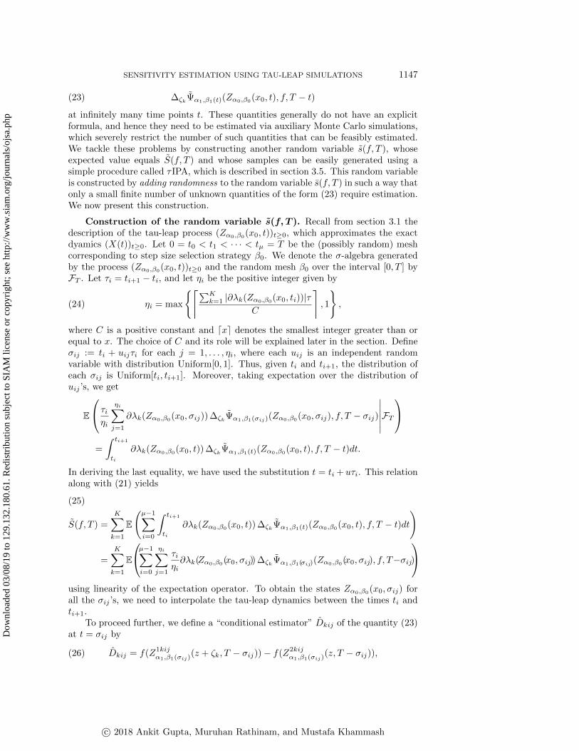
at infinitely many time points t. These quantities generally do not have an explicitformula, and hence they need to be estimated via auxiliary Monte Carlo simulations,which severely restrict the number of such quantities that can be feasibly estimated.We tackle these problems by constructing another random variable \~s(f, T ), whoseexpected value equals \~S(f, T ) and whose samples can be easily generated using asimple procedure called \tau IPA, which is described in section 3.5. This random variableis constructed by adding randomness to the random variable \=s(f, T ) in such a way thatonly a small finite number of unknown quantities of the form (23) require estimation.We now present this construction.
Construction of the random variable \~\bfits (\bfitf , \bfitT ). Recall from section 3.1 thedescription of the tau-leap process (Z\alpha 0,\beta 0
(x0, t))t\geq 0, which approximates the exactdyamics (X(t))t\geq 0. Let 0 = t0 < t1 < \cdot \cdot \cdot < t\mu = T be the (possibly random) meshcorresponding to step size selection strategy \beta 0. We denote the \sigma -algebra generatedby the process (Z\alpha 0,\beta 0
(x0, t))t\geq 0 and the random mesh \beta 0 over the interval [0, T ] by\scrF T . Let \tau i = ti+1 - ti, and let \eta i be the positive integer given by
\eta i = max
\Biggl\{ \Biggl\lceil \sum Kk=1 | \partial \lambda k(Z\alpha 0,\beta 0(x0, ti))| \tau
C
\Biggr\rceil , 1
\Biggr\} ,(24)
where C is a positive constant and \lceil x\rceil denotes the smallest integer greater than orequal to x. The choice of C and its role will be explained later in the section. Define\sigma ij := ti + uij\tau i for each j = 1, . . . , \eta i, where each uij is an independent randomvariable with distribution Uniform[0, 1]. Thus, given ti and ti+1, the distribution ofeach \sigma ij is Uniform[ti, ti+1]. Moreover, taking expectation over the distribution ofuij 's, we get
\BbbE
\left( \tau i\eta i
\eta i\sum j=1
\partial \lambda k(Z\alpha 0,\beta 0(x0, \sigma ij))\Delta \zeta k
\~\Psi \alpha 1,\beta 1(\sigma ij)(Z\alpha 0,\beta 0(x0, \sigma ij), f, T - \sigma ij)
\bigm| \bigm| \bigm| \bigm| \bigm| \bigm| \scrF T
\right) =
\int ti+1
ti
\partial \lambda k(Z\alpha 0,\beta 0(x0, t))\Delta \zeta k
\~\Psi \alpha 1,\beta 1(t)(Z\alpha 0,\beta 0(x0, t), f, T - t)dt.
In deriving the last equality, we have used the substitution t = ti + u\tau i. This relationalong with (21) yields
\~S(f, T ) =
K\sum k=1
\BbbE
\Biggl( \mu - 1\sum i=0
\int ti+1
ti
\partial \lambda k(Z\alpha 0,\beta 0(x0, t))\Delta \zeta k
\~\Psi \alpha 1,\beta 1(t)(Z\alpha 0,\beta 0(x0, t), f, T - t)dt
\Biggr) (25)
=
K\sum k=1
\BbbE
\left( \mu - 1\sum i=0
\eta i\sum j=1
\tau i\eta i\partial \lambda k(Z\alpha 0,\beta 0
(x0, \sigma ij))\Delta \zeta k\~\Psi \alpha 1,\beta 1(\sigma ij)(Z\alpha 0,\beta 0
(x0, \sigma ij), f, T - \sigma ij)
\right) using linearity of the expectation operator. To obtain the states Z\alpha 0,\beta 0(x0, \sigma ij) forall the \sigma ij 's, we need to interpolate the tau-leap dynamics between the times ti andti+1.
To proceed further, we define a ``conditional estimator"" \^Dkij of the quantity (23)at t = \sigma ij by
(26) \^Dkij = f(Z1kij\alpha 1,\beta 1(\sigma ij)
(z + \zeta k, T - \sigma ij)) - f(Z2kij\alpha 1,\beta 1(\sigma ij)
(z, T - \sigma ij)),
c\bigcirc 2018 Ankit Gupta, Muruhan Rathinam, and Mustafa Khammash
Dow
nloa
ded
03/0
8/19
to 1
29.1
32.1
80.6
1. R
edis
trib
utio
n su
bjec
t to
SIA
M li
cens
e or
cop
yrig
ht; s
ee h
ttp://
ww
w.s
iam
.org
/jour
nals
/ojs
a.ph
p

1148 A. GUPTA, M. RATHINAM, AND M. KHAMMASH
where z = Z\alpha 0,\beta 0(x0, \sigma ij) and Z1kij and Z2kij are instances of tau-leap approxima-
tions of the exact dynamics starting at initial states (z + \zeta k) and z, respectively.Both these tau-leap processes use the same method \alpha 1 and the same step size selec-tion strategy \beta 1(\sigma ij). Moreover, conditioned on Z\alpha 0,\beta 0(x0, \sigma ij) and \sigma ij , the processesZ1kij , Z2kij and the step size selection strategy \beta 1(\sigma ij) are independent of the processZ\alpha 0,\beta 0
and the step size selection strategy \beta 0. Therefore, it is immediate that
(27) \BbbE ( \^Dkij | Z\alpha 0,\beta 0(x0, \sigma ij), \sigma ij) = \Delta \zeta k\~\Psi \alpha 1,\beta 1(\sigma ij)(Z\alpha 0,\beta 0(x0, \sigma ij), f, T - \sigma ij),
and hence from (25), we obtain the following representation for \~S(f, T ):
\~S(f, T ) =
K\sum k=1
\BbbE
\left( \mu - 1\sum i=0
\eta i\sum j=1
\tau i\eta i\partial \lambda k(Z\alpha 0,\beta 0
(x0, \sigma ij)) \^Dkij
\right) .(28)
An estimator for \~S(f, T ) based on this formula can require several computations of\^Dkij . Since each evaluation of \^Dkij is computationally expensive, we would like tocontrol the total number of these evaluations by randomizing the decision of whether\^Dkij should be evaluated at time \sigma ij or not. Moreover, this randomization must beperformed without introducing a bias in the estimator. We now describe this process.
Define Rkij and Pkij by
Rkij = \partial \lambda k(Z\alpha 0,\beta 0(x0, \sigma ij))\tau i and Pkij =
\biggl( | Rkij | C\eta i
\biggr) \wedge 1,(29)
and let \rho kij be an independent \{ 0, 1\} -valued random variable whose distribution isBernoulli with parameter Pkij . Since \BbbE (\rho kij | Z\alpha 0,\beta 0
(x0, \sigma ij),\scrF T ) = Pkij , we have that
\~S(f, T ) =
K\sum k=1
\BbbE
\left( \mu - 1\sum i=0
\eta i\sum j=1
\biggl( Rkij
Pkij\eta i
\biggr) \rho kij \^Dkij
\right) ,(30)
where we define Rkij/Pkij to be 0 when Rkij = 0. This formula suggests that \~S(f, T )can be estimated, without any bias, using realizations of the random variable
\~s(f, T ) =
K\sum k=1
\mu - 1\sum i=0
\eta i\sum j=1
\biggl( Rkij
Pkij\eta i
\biggr) \rho kij \^Dkij .(31)
In generating each realization of \~s(f, T ), the computation of \^Dkij is only neededif the Bernoulli random variable \rho kij is 1. Therefore, if we can effectively controlthe number of such \rho kij 's, then we can efficiently generate realizations of \~s(f, T ).This can be achieved using the positive parameter C (see (24) and (29)) as we soonexplain. Based on the construction outlined above, we provide a method in section3.5 for obtaining realizations of the random variable \~s(f, T ). We call this method the\tau IPA to emphasize the fact that \~s(f, T ) is essentially an approximation of the integral(22). Using \tau IPA, we can efficiently generate realizations s1, s2, . . . , sN of \~s(f, T ) andapproximately estimate the parameter sensitivity \~S(f, T ) with the estimator (6).
Minimizing the variance of \~\bfits (\bfitf , \bfitT ). To improve the efficiency of \tau IPA, wemust minimize the additional variance due to the extra randomness that has beenadded to the random variable \=s(f, T ) (22) to obtain \~s(f, T ). Since \BbbE (\~s(f, T )| \scrF T ) =\=s(f, T ), this additional variance is equal to Var(\~s(f, T )| \scrF T ), and in order to reduce
c\bigcirc 2018 Ankit Gupta, Muruhan Rathinam, and Mustafa Khammash
Dow
nloa
ded
03/0
8/19
to 1
29.1
32.1
80.6
1. R
edis
trib
utio
n su
bjec
t to
SIA
M li
cens
e or
cop
yrig
ht; s
ee h
ttp://
ww
w.s
iam
.org
/jour
nals
/ojs
a.ph
p

SENSITIVITY ESTIMATION USING TAU-LEAP SIMULATIONS 1149
this quantity, we focus on reducing the conditional variance Var( \^Dkij | \scrF T ). Recall
that \^Dkij is given by (26), and for convenience, we abbreviate Zlkij\alpha 1,\beta 1(\sigma ij)
by Zl for
l = 1, 2. The reduction in this conditional variance can be accomplished by tightlycoupling the pair of processes (Z1, Z2). For this purpose, we use the split-coupling(see [2]) specified by
Z1(t) = (Z\alpha 0,\beta 0(x0, \sigma ij) + \zeta k) +
K\sum k=1
Yk
\biggl( \int t
0
\lambda k(Z1(\alpha (s)), \theta ) \wedge \lambda k(Z
2(\alpha (s)), \theta )ds
\biggr) \zeta k
(32)
+
K\sum k=1
Y(1)k
\biggl( \int t
0
\bigl( \lambda k(Z
1(\alpha ((s)), \theta ) - \lambda k(Z1(\alpha (s)), \theta ) \wedge \lambda k(Z
2(\alpha (s)), \theta )\bigr) ds
\biggr) \zeta k
Z2(t) = Z\alpha 0,\beta 0(x0, \sigma ij) +
K\sum k=1
Yk
\biggl( \int t
0
\lambda k(Z1(\alpha (s)), \theta ) \wedge \lambda k(Z
2(\alpha (s)), \theta )ds
\biggr) \zeta k
(33)
+
K\sum k=1
Y(2)k
\biggl( \int t
0
\bigl( \lambda k(Z
2(\alpha ((s)), \theta ) - \lambda k(Z1(\alpha (s)), \theta ) \wedge \lambda k(Z
2(\alpha (s)), \theta )\bigr) ds
\biggr) \zeta k
where \{ Yk, Y(1)k , Y
(2)k : k = 1, . . . ,K\} is an independent family of unit rate Poisson
processes. Here \alpha (s) = ti for ti \leq s < ti+1, and \{ t0, t1, t2, . . . \} is the sequence of leaptimes of the pair of processes (Z1, Z2) jointly simulated with the tau-leap scheme(\alpha 1, \beta 1(t)).
Controlling the number of nonzero \bfitrho \bfitk \bfiti \bfitj 's. We now discuss how the positiveparameter C can be selected to control the total number of \rho kij 's that assume the
value 1 in (31), which is \rho tot =\sum K
k=1
\sum \mu - 1i=1
\sum \eta i
j=1 \rho kij . This is the number of \^Dkij 'sthat are required to obtain a realization of \~s(f, T ). It is immediate that given thesigma field \scrF T , \rho tot is a \BbbN 0-valued random variable whose expectation is given by
\BbbE (\rho tot| \scrF T ) =
K\sum k=1
\mu - 1\sum i=1
\eta i\sum j=1
\BbbE (Pkij | \scrF T ) =
K\sum k=1
\mu - 1\sum i=1
\eta i\sum j=1
\BbbE \biggl[ \biggl( | Rkij | C\eta i
\biggr) \wedge 1
\bigm| \bigm| \bigm| \bigm| \scrF T
\biggr] .
Using a \wedge b \leq a and
\BbbE (| Rkij | | \scrF T ) =
\int ti+1
ti
| \partial \lambda k(Z\alpha 0,\beta 0(x0, t))| dt,
we obtain
\BbbE (\rho tot) = \BbbE (\BbbE (\rho tot| \scrF T )) \leq 1
C
K\sum k=1
\BbbE
\Biggl( \int T
0
| \partial \lambda k(Z\alpha 0,\beta 0(x0, t))| dt
\Biggr) .(34)
We choose a positive integer M0 and set
C =1
M0
K\sum k=1
\BbbE
\Biggl( \int T
0
| \partial \lambda k(Z\alpha 0,\beta 0(x0, t))| dt
\Biggr) ,(35)
where the expectation can be approximately estimated using N0 tau-leap simulationsof the dynamics in the time interval [0, T ]. Such a choice ensures that \rho tot is boundedabove by M0 on average. In most cases, we can expect that Rkij to be close to
c\bigcirc 2018 Ankit Gupta, Muruhan Rathinam, and Mustafa Khammash
Dow
nloa
ded
03/0
8/19
to 1
29.1
32.1
80.6
1. R
edis
trib
utio
n su
bjec
t to
SIA
M li
cens
e or
cop
yrig
ht; s
ee h
ttp://
ww
w.s
iam
.org
/jour
nals
/ojs
a.ph
p

1150 A. GUPTA, M. RATHINAM, AND M. KHAMMASH
\partial \lambda k(Z\alpha 0,\beta 0(x0, ti))\tau i, and so the choice of \eta i automatically ensures that | Rkij | \leq C\eta i.
Hence inequality (34) is almost exact, and with C chosen as (35), we have \BbbE (\rho tot) \approx M0. Therefore, M0 can be interpreted as the expected number of coupled auxiliarypaths (32)--(33) needed to obtain a realization of \~s(f, T ). This parameter is in thehands of the user, and it plays the same role as in PPA (see section 2.2); namely, itallows one to select the trade-off between the computational cost \scrC (\tau IPA) and thevariance \scrV (\tau IPA). A higher value of M0 reduces the variance while simultaneouslyincreasing the computational cost. Hence, it is difficult to ascertain the effect of M0
on the overall estimation cost, which depends on the product \scrC (\tau IPA)\scrV (\tau IPA) (see(10)). Numerical examples suggest that for low values of M0, the overall estimationcost decreases gradually with increase in M0, but this trend reverses for higher valuesof M0 (see section 4). More work is needed to examine if this pattern persists moregenerally and how one can select the optimal value of M0. Note, however, that \tau IPAwill provide an unbiased estimator for \~S(f, T ) (21) regardless of the choice of M0.Hence, the accuracy of \tau IPA does not vary much with M0, which is also seen in thenumerical examples.
3.5. \bfittau IPA. We now provide a detailed description of the method \tau IPA, whichproduces realizations of the random variable \~s(f, T ) defined by (31). Computingthe empirical mean (6) of these realizations estimates the approximate parametersensitivity \~S(f, T ). Throughout this section, we assume that the function rand()returns independent samples from the distribution Uniform[0, 1].
The method \tau IPA can be adapted to work with any tau-leap scheme, but for con-creteness, we assume that an explicit tau-leap scheme is used for all the simulations.This means that the current state z and time t are sufficient to determine the distri-butions of the next time step \tau and the vector of reaction firings \~R = ( \~R1, . . . , \~RK) inthe time interval [t, t+\tau ). We suppose that a sample from these two distributions canbe obtained using the methods GetTau(z, t, T )2 and GetReactionFirings(z, \tau ),respectively. If we use the simplest tau-leap scheme given in [20], then reaction firingscan be generated as
\~Rk = Poisson(\lambda k(z)\tau )(36)
for k = 1, . . . ,K, where the function Poisson(r) generates an independent Poissonrandom variable with mean r. Once we have the reaction firings \~R = ( \~R1, . . . , \~RK),
the state at time (t+ \tau ) is given by z\prime = (z +\sum K
k=1\~Rk\zeta k), and for any intermediate
time point \sigma \in (t, t + \tau ), the state \^z can be obtained using the ``Poisson bridge""interpolation (see [28]). However, this interpolation approach is equivalent to setting
\^z = (z+\sum K
k=1\~R(1)k \zeta k) and z\prime = (\^z+
\sum Kk=1
\~R(2)k \zeta k), where \~R(1) = ( \~R
(1)1 , . . . , \~R
(1)K ) and
\~R(2) = ( \~R(2)1 , . . . , \~R
(2)K ) are reaction firing vectors generated according to (36) with \tau
replaced by (\sigma - t) and (t+\tau - \sigma ), respectively. This idea can be easily generalized toobtain the interpolated states \^z1, . . . , \^z\eta at \eta intermediate times \sigma 1, . . . , \sigma \eta \in (t, t+ \tau )sorted in ascending order, i.e., \sigma 1 < \cdot \cdot \cdot < \sigma \eta .
Let Z denote the tau-leap process approximating the reaction dynamics with ini-tial state x0. Our first task is to select a normalization parameter C according to(35) by estimating the expectation in the formula using N0 simulations of the pro-cess Z. This is done using the function Select-Normalizing-Constant(x0,M0, T )
2We allow the step size selection to depend on both the current time t and the final time T . Thisis especially important for simulating the auxiliary paths that are required to compute the \^Dki's in(31) (see sections 3.3 and 3.4).
c\bigcirc 2018 Ankit Gupta, Muruhan Rathinam, and Mustafa Khammash
Dow
nloa
ded
03/0
8/19
to 1
29.1
32.1
80.6
1. R
edis
trib
utio
n su
bjec
t to
SIA
M li
cens
e or
cop
yrig
ht; s
ee h
ttp://
ww
w.s
iam
.org
/jour
nals
/ojs
a.ph
p
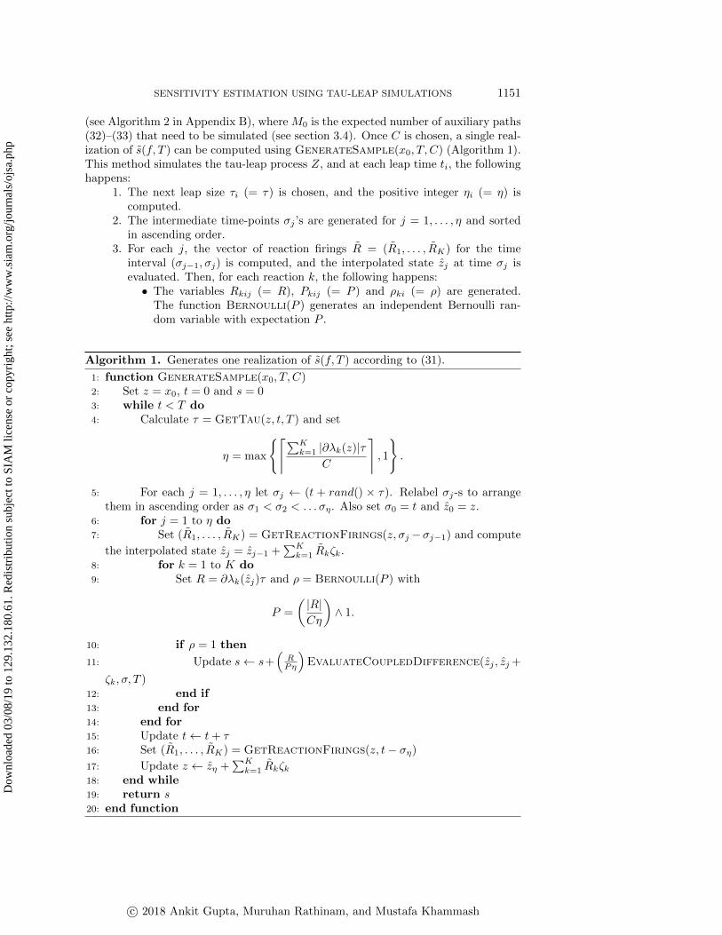
SENSITIVITY ESTIMATION USING TAU-LEAP SIMULATIONS 1151
(see Algorithm 2 in Appendix B), where M0 is the expected number of auxiliary paths(32)--(33) that need to be simulated (see section 3.4). Once C is chosen, a single real-ization of \~s(f, T ) can be computed using GenerateSample(x0, T, C) (Algorithm 1).This method simulates the tau-leap process Z, and at each leap time ti, the followinghappens:
1. The next leap size \tau i (= \tau ) is chosen, and the positive integer \eta i (= \eta ) iscomputed.
2. The intermediate time-points \sigma j 's are generated for j = 1, . . . , \eta and sortedin ascending order.
3. For each j, the vector of reaction firings \~R = ( \~R1, . . . , \~RK) for the timeinterval (\sigma j - 1, \sigma j) is computed, and the interpolated state \^zj at time \sigma j isevaluated. Then, for each reaction k, the following happens:\bullet The variables Rkij (= R), Pkij (= P ) and \rho ki (= \rho ) are generated.
The function Bernoulli(P ) generates an independent Bernoulli ran-dom variable with expectation P .
Algorithm 1. Generates one realization of \~s(f, T ) according to (31).
1: function GenerateSample(x0, T, C)2: Set z = x0, t = 0 and s = 03: while t < T do4: Calculate \tau = GetTau(z, t, T ) and set
\eta = max
\Biggl\{ \Biggl\lceil \sum Kk=1 | \partial \lambda k(z)| \tau
C
\Biggr\rceil , 1
\Biggr\} .
5: For each j = 1, . . . , \eta let \sigma j \leftarrow (t + rand() \times \tau ). Relabel \sigma j-s to arrangethem in ascending order as \sigma 1 < \sigma 2 < . . . \sigma \eta . Also set \sigma 0 = t and \^z0 = z.
6: for j = 1 to \eta do7: Set ( \~R1, . . . , \~RK) = GetReactionFirings(z, \sigma j - \sigma j - 1) and compute
the interpolated state \^zj = \^zj - 1 +\sum K
k=1\~Rk\zeta k.
8: for k = 1 to K do9: Set R = \partial \lambda k(\^zj)\tau and \rho = Bernoulli(P ) with
P =
\biggl( | R| C\eta
\biggr) \wedge 1.
10: if \rho = 1 then
11: Update s\leftarrow s+\Bigl(
RP\eta
\Bigr) EvaluateCoupledDifference(\^zj , \^zj+
\zeta k, \sigma , T )12: end if13: end for14: end for15: Update t\leftarrow t+ \tau 16: Set ( \~R1, . . . , \~RK) = GetReactionFirings(z, t - \sigma \eta )
17: Update z \leftarrow \^z\eta +\sum K
k=1\~Rk\zeta k
18: end while19: return s20: end function
c\bigcirc 2018 Ankit Gupta, Muruhan Rathinam, and Mustafa Khammash
Dow
nloa
ded
03/0
8/19
to 1
29.1
32.1
80.6
1. R
edis
trib
utio
n su
bjec
t to
SIA
M li
cens
e or
cop
yrig
ht; s
ee h
ttp://
ww
w.s
iam
.org
/jour
nals
/ojs
a.ph
p
1152 A. GUPTA, M. RATHINAM, AND M. KHAMMASH
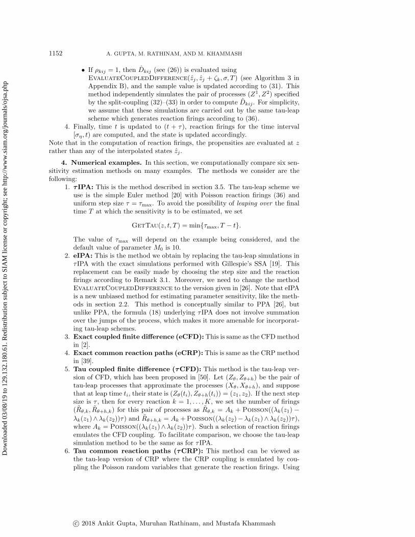
\bullet If \rho kij = 1, then \^Dkij (see (26)) is evaluated usingEvaluateCoupledDifference(\^zj , \^zj + \zeta k, \sigma , T ) (see Algorithm 3 inAppendix B), and the sample value is updated according to (31). Thismethod independently simulates the pair of processes (Z1, Z2) specifiedby the split-coupling (32)--(33) in order to compute \^Dkij . For simplicity,we assume that these simulations are carried out by the same tau-leapscheme which generates reaction firings according to (36).
4. Finally, time t is updated to (t + \tau ), reaction firings for the time interval[\sigma \eta , t) are computed, and the state is updated accordingly.
Note that in the computation of reaction firings, the propensities are evaluated at zrather than any of the interpolated states \^zj .
4. Numerical examples. In this section, we computationally compare six sen-sitivity estimation methods on many examples. The methods we consider are thefollowing:
1. \bfittau IPA: This is the method described in section 3.5. The tau-leap scheme weuse is the simple Euler method [20] with Poisson reaction firings (36) anduniform step size \tau = \tau max. To avoid the possibility of leaping over the finaltime T at which the sensitivity is to be estimated, we set
GetTau(z, t, T ) = min\{ \tau max, T - t\} .
The value of \tau max will depend on the example being considered, and thedefault value of parameter M0 is 10.
2. eIPA: This is the method we obtain by replacing the tau-leap simulations in\tau IPA with the exact simulations performed with Gillespie's SSA [19]. Thisreplacement can be easily made by choosing the step size and the reactionfirings according to Remark 3.1. Moreover, we need to change the methodEvaluateCoupledDifference to the version given in [26]. Note that eIPAis a new unbiased method for estimating parameter sensitivity, like the meth-ods in section 2.2. This method is conceptually similar to PPA [26], butunlike PPA, the formula (18) underlying \tau IPA does not involve summationover the jumps of the process, which makes it more amenable for incorporat-ing tau-leap schemes.
3. Exact coupled finite difference (eCFD): This is same as the CFDmethodin [2].
4. Exact common reaction paths (eCRP): This is same as the CRP methodin [39].
5. Tau coupled finite difference (\bfittau CFD): This method is the tau-leap ver-sion of CFD, which has been proposed in [50]. Let (Z\theta , Z\theta +h) be the pair oftau-leap processes that approximate the processes (X\theta , X\theta +h), and supposethat at leap time ti, their state is (Z\theta (ti), Z\theta +h(ti)) = (z1, z2). If the next stepsize is \tau , then for every reaction k = 1, . . . ,K, we set the number of firings( \~R\theta ,k, \~R\theta +h,k) for this pair of processes as \~R\theta ,k = Ak + Poisson((\lambda k(z1) - \lambda k(z1)\wedge \lambda k(z2))\tau ) and \~R\theta +h,k = Ak +Poisson((\lambda k(z2) - \lambda k(z1)\wedge \lambda k(z2))\tau ),where Ak = Poisson((\lambda k(z1)\wedge \lambda k(z2))\tau ). Such a selection of reaction firingsemulates the CFD coupling. To facilitate comparison, we choose the tau-leapsimulation method to be the same as for \tau IPA.
6. Tau common reaction paths (\bfittau CRP): This method can be viewed asthe tau-leap version of CRP where the CRP coupling is emulated by cou-pling the Poisson random variables that generate the reaction firings. Using
c\bigcirc 2018 Ankit Gupta, Muruhan Rathinam, and Mustafa Khammash
Dow
nloa
ded
03/0
8/19
to 1
29.1
32.1
80.6
1. R
edis
trib
utio
n su
bjec
t to
SIA
M li
cens
e or
cop
yrig
ht; s
ee h
ttp://
ww
w.s
iam
.org
/jour
nals
/ojs
a.ph
p

SENSITIVITY ESTIMATION USING TAU-LEAP SIMULATIONS 1153
the same notation as before, if (Z\theta (ti), Z\theta +h(ti)) = (z1, z2) and the nextstep size is \tau , then we set the number of firings ( \~R\theta ,k, \~R\theta +h,k) as \~R\theta ,k =
Poisson(\lambda k(z1)\tau , k) and \~R\theta +h,k = Poisson(\lambda k(z2)\tau , k) for every reactionk = 1, . . . ,K. Here we assume that there are K parallel streams of indepen-dent Uniform[0, 1] random variables (see [39]), and the method Poisson(r, k)uses the uniform random variable from the kth stream for generating thePoisson random variable with mean r. As for \tau CFD, the tau-leap simulationmethod is the same as for \tau IPA.
In all the finite difference schemes, we use perturbation size h = 0.1, and we centerthe parameter perturbations to obtain better accuracy. This centering can be easilyachieved by substituting \theta with (\theta - h/2) and (\theta +h) with (\theta +h/2) in the expression(11) and also in the definition of the coupled processes. Since we use Poisson randomvariables to generate the reaction firings for tau-leap simulations, it is possible thatsome state-components become negative during the simulation run. In this paper, wedeal with this problem rather crudely by setting the negative state-components to 0.We have checked that this does not cause a significant loss of accuracy because thestate-components become negative very rarely.
Note that among the methods considered here, eIPA is the only unbiased sensitivityestimation method. All the other methods are biased either due to a finite-differenceapproximation of the derivative (eCFD and eCRP) or due to tau-leap approxima-tion of the sample paths (\tau IPA) or due to both these reasons (\tau CFD and \tau CRP).In the examples, we apply each sensitivity estimation method \scrX with a sample sizeof N = 105 and compute the estimator mean \^\mu N (6), the standard deviation \^\sigma N
(9), the relative standard deviation RSD(\scrX ), and the computational cost per sample\scrC (\scrX ) (see section 2). Assume that the exact sensitivity value is s0, which is known.We compare the different estimation methods using the following two quantities---thepercentage relative error (RE) defined by
RE =
\bigm| \bigm| \bigm| \bigm| \^\mu N - s0s0
\bigm| \bigm| \bigm| \bigm| \times 100(37)
and the RSD adjusted computational cost (RSDCC) defined by
RSDCC = (RSD(\scrX ))2\scrC (\scrX ).(38)
The first quantity RE measures the accuracy of a method, while the second quan-tity RSDCC determines the overall computational time that will be required by themethod to yield an estimate with the desired statistical precision (see (10)).
Our numerical results will show that the exact schemes (eIPA, eCFD, and eCRP)usually have a higher RSDCC than their tau-leap counterparts (\tau IPA, \tau CFD, and\tau CRP), but expectedly their RE is lower. Generally, the RE for eIPA is smaller thanboth eCFD and eCRP because of its unbiasedness, and this advantage in accuracyoften persists when we compare \tau IPA with \tau CFD and \tau CRP. It can be seen that inmost of the cases, the sample variance \scrV (\scrX ) or the estimator standard deviation (9)remains of similar magnitude when we switch from an exact scheme to its tau-leapversion (see Appendix B). This supports our claim in section 2.3 that substitutingexact paths with tau-leap trajectories allows one to trade off bias with computationalcosts, and this trade-off relationship is somewhat ``orthogonal"" to other trade-offrelationships shown in Table 1.
In all the examples below, the propensity functions \lambda k's for all the reactions havethe mass-action form [3] unless stated otherwise. Also, \partial always denotes the partialderivative w.r.t. the designated sensitive parameter \theta .
c\bigcirc 2018 Ankit Gupta, Muruhan Rathinam, and Mustafa Khammash
Dow
nloa
ded
03/0
8/19
to 1
29.1
32.1
80.6
1. R
edis
trib
utio
n su
bjec
t to
SIA
M li
cens
e or
cop
yrig
ht; s
ee h
ttp://
ww
w.s
iam
.org
/jour
nals
/ojs
a.ph
p

1154 A. GUPTA, M. RATHINAM, AND M. KHAMMASH
4.1. Single-species birth-death model. Our first example is a simple birth-death model in which a single species \scrS is created and destroyed according to thefollowing two reactions:
\emptyset \theta 1 - \rightarrow \scrS \theta 2 - \rightarrow \emptyset .
Let \theta 1 = 10, \theta 2 = 0.1, and assume that the sensitive parameter is \theta = \theta 2. Let(X(t))t\geq 0 be the Markov process representing the reaction dynamics. Assume thatX(0) = 0. For f(x) = x, we wish to estimate
S\theta (f, T ) = \partial \BbbE (f(X(T ))) = \partial \BbbE (X(T ))
for T = 5 and T = 10. For this example, we set \tau max = 0.5. For each T , we estimatethe sensitivity using all the six methods, and the results are displayed in Table 3 inAppendix B. For this network, we can compute the sensitivity S\theta (f, T ) exactly asthe propensity functions are affine. These exact values are stated in the caption ofTable 3, and they allow us to compute the RE of a method according to (37). Wealso compute the RSDCC3 for each method using (38), and we compare these RE andRSDCC values for all the methods in Figure 1A. From these comparisons, we canmake the following observations: (1) The exact methods are typically more accuratethan the tau-leap methods, but they are usually more computationally demanding.(2) For T = 5, eCFD/eCRP are far more accurate than \tau CFD/\tau CRP, suggesting thatthe two sources of bias (finite difference and tau-leap approximations) are additivein nature. However, the same is not true for T = 10. (3) For both the cases T = 5and T = 10, \tau IPA outperforms \tau CFD/\tau CRP in terms of accuracy even though it isslightly more computationally expensive. The same is true when we compare eIPAwith eCFD/eCRP.
In Figure 1B, we numerically analyze the performance of \tau IPA w.r.t. its two keyparameters---the expected number of auxiliary paths M0 and the maximum tau-leapstep size \tau max. We see that RE is fairly insensitive to variations in M0, while RSDCCfirst decreases withM0 up to a certain point and then starts increasing withM0. As weare using a first-order explicit tau-leap scheme, it is unsurprising that RE increasesalmost linearly with \tau max. However, importantly, RSDCC decreases exponentiallywith \tau max, which makes it possible to use tau-leap simulations to trade off a smallamount of accuracy for a large gain in computational efficiency with \tau IPA.
Observe that if we scale the production rate \theta 1 by the system size or volumeparameter V , then the concentration process, derived by dividing the copy-numbercounts X(t) by V , converges to a deterministic ODE limit as V \rightarrow \infty (see Chapter 11in [14]). Often, it is of interest to determine how the performance of various sensitivityestimation methods scales with the volume parameter V . We investigate this issue forthe exact schemes (eIPA, eCFD, and eCRP) in Figure 2 by numerically examining thedependence of their RSD, RSDCC, and RE on V . Here we set the expected numberof auxiliary paths M0 for eIPA to be equal to V . Note that RSD for finite-differenceschemes (eCFD/eCRP) scales like 1/
\surd V as was proved in [44] and consequently their
RSDCC is of order 1 because the computational time per sample, which is proportionalto the number of reaction events per unit time interval, is of order V . Similar to thesefinite difference schemes, the RSD for eIPA also scales like 1/
\surd V , but its RSDCC is
of order V , as its computational time per sample is of order V 2 because to generate
3All the computations in this paper were performed using C++ programs on an Apple machinewith a 2.9-GHz Intel Core i5 processor.
c\bigcirc 2018 Ankit Gupta, Muruhan Rathinam, and Mustafa Khammash
Dow
nloa
ded
03/0
8/19
to 1
29.1
32.1
80.6
1. R
edis
trib
utio
n su
bjec
t to
SIA
M li
cens
e or
cop
yrig
ht; s
ee h
ttp://
ww
w.s
iam
.org
/jour
nals
/ojs
a.ph
p

SENSITIVITY ESTIMATION USING TAU-LEAP SIMULATIONS 1155
T = 5 T = 10A
BUnbiased UnbiasedeIPA IPA eCFD CFD eCRP CRP
0
1
2
3
4
5
RE%
10-7
10-6
10-5
RSD
CC
RE%RSDCC
eIPA IPA eCFD CFD eCRP CRP0
0.5
1
1.5
2
RE%
10-7
10-6
10-5
RSD
CC
RE%RSDCC
100 101 102 103M0
0
1
2
3
4
5
RE%
10-6
10-5
10-4RSD
CC
RE%RSDCC
0 0.2 0.4 0.6 0.8 1max
0
0.2
0.4
0.6
0.8
1
1.2
1.4
RE%
10-6
10-5
10-4
RSD
CC
RE%VACC
Fig. 1. Birth-death model: Panel A compares the various sensitivity estimation methods interms of the percentage relative error (RE) (calibrated with the left y-axis in linear scale) and therelative standard deviation adjusted computational cost (RSDCC) (calibrated with the right y-axisin log scale). The sensitivities are estimated for T = 5 and 10 using N = 105 samples. In panelB, we study how the performance of \tau IPA depends on parameters M0 (expected number of auxiliarypaths) and \tau max (maximum tau-leap step size) for the case T = 10.
100 101 102 103
Volume (V)
10-3
10-2
10-1
100
101
RSD
eIPAeCFDeCRP
100 101 102 103
Volume (V)
10-6
10-5
10-4
10-3
10-2
10-1
RSD
CC eIPA
eCFDeCRP
100 101 102 103
Volume (V)
0
0.5
1
1.5
2
2.5
RE%
eIPAeCFDeCRP
Fig. 2. Birth-death model: In this figure, we examine how the performance of the exact schemes(eIPA, eCFD, and eCRP) varies with the system size represented by volume V . We study thecase T = 10 by replacing the production rate \theta 1 by \theta 1V . For eIPA, we set the expected number ofauxiliary paths as M0 = V . The three plots compare the three exact schemes in terms of their relativestandard deviation (RSD), the relative standard deviation adjusted computational cost (RSDCC),and the percentage relative error (RE). Note that the x-axis for volume V is in log scale that andthe y-axis for RSD and RSDCC is in log scale but for RE is in linear scale.
each sample for eIPA, M0 = V auxiliary paths need to be simulated in addition to themain sample path. This computational disadvantage of eIPA is compensated by thefact that accuracy of eIPA improves with volume (i.e., RE decreases with volume),while for the finite difference schemes, it is almost a constant. These numerical results
c\bigcirc 2018 Ankit Gupta, Muruhan Rathinam, and Mustafa Khammash
Dow
nloa
ded
03/0
8/19
to 1
29.1
32.1
80.6
1. R
edis
trib
utio
n su
bjec
t to
SIA
M li
cens
e or
cop
yrig
ht; s
ee h
ttp://
ww
w.s
iam
.org
/jour
nals
/ojs
a.ph
p
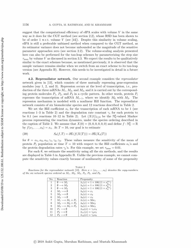
1156 A. GUPTA, M. RATHINAM, AND M. KHAMMASH
suggest that the computational efficiency of eIPA scales with volume V in the sameway as it does for the CGT method (see section 2.2), whose RSD has been shown tobe of order 1 w.r.t. volume V (see [44]). Despite this similarity in volume scaling,eIPA is still a preferable unbiased method when compared to the CGT method, asits estimator variance does not become unbounded as the magnitude of the sensitiveparameter approaches zero (see section 2.2). The volume-scaling analysis presentedhere can also be performed for the tau-leap schemes by parameterizing the step size\tau max by volume V as discussed in section 3.3. We expect the results to be qualitativelysimilar to the exact schemes because, as mentioned previously, it is observed that thesample variance remains similar when we switch from an exact scheme to its tau-leapversion (see Appendix B). However, this needs to be investigated in detail in a futurework.
4.2. Repressilator network. Our second example considers the repressilatornetwork given in [13], which consists of three mutually repressing gene-expressionmodules (say 1, 2, and 3). Repression occurs at the level of transcription, i.e., pro-duction of the three mRNAs M1, M2, and M3, and it is carried out by the correspond-ing protein molecules P1, P2, and P3 in a cyclic pattern. In other words, protein Pi
represses the transcription of mRNA Mi - 1, where we identify M0 with M3. Therepression mechanism is modeled with a nonlinear Hill function. The repressilatornetwork consists of six biomolecular species and 12 reactions described in Table 2.
We set the Hill coefficient \alpha i for the transcription of each mRNA to be 1 (seereactions 1--3 in Table 2) and the degradation rate constant \gamma i for each protein tobe 0.1 (see reactions 10--12 in Table 2). Let (X(t))t\geq 0 be the \BbbN 6
0-valued Markovprocess representing the reaction dynamics, under the species ordering described inthe caption of Table 2. We assume that X(0) = (0, 0, 0, 0, 0, 0) and define f : \BbbN 6
0 \rightarrow \BbbR by f(x1, . . . , x6) = x4. At T = 10, our goal is to estimate
S\theta (f, T ) = \partial \BbbE (f(X(T ))) = \partial \BbbE (X4(T ))(39)
for \theta = \alpha 1, \alpha 2, \alpha 3, \gamma 1, \gamma 2, \gamma 3. These values measure the sensitivity of the mean ofprotein P1 population at time T = 10 with respect to the Hill coefficients \alpha i's andthe protein degradation rates \gamma j 's. For this example, we set \tau max = 0.01.
For each \theta , we estimate the sensitivity using all the six methods, and the resultsare displayed in Table 5 in Appendix B. Unlike the previous example, we cannot com-pute the sensitivity values exactly because of nonlinearity of some of the propensity
Table 2Reactions for the repressilator network [13]. Here x = (x1, . . . , x6) denotes the copy-numbers
of the six network species ordered as M1, M2, M3, P4, P5, and P6.
No. Reaction Propensity1 \emptyset - \rightarrow M1 \lambda 1(x) = 1 + 100/(1 + x\alpha 1
5 )2 \emptyset - \rightarrow M2 \lambda 2(x) = 1 + 100/(1 + x\alpha 2
6 )3 \emptyset - \rightarrow M3 \lambda 3(x) = 1 + 100/(1 + x\alpha 3
4 )4 M1 - \rightarrow \emptyset \lambda 4(x) = x1
5 M2 - \rightarrow \emptyset \lambda 5(x) = x2
6 M3 - \rightarrow \emptyset \lambda 6(x) = x3
7 M1 - \rightarrow M1 + P1 \lambda 7(x) = 50x1
8 M2 - \rightarrow M2 + P2 \lambda 8(x) = 50x2
9 M3 - \rightarrow M3 + P3 \lambda 9(x) = 50x3
10 P1 - \rightarrow \emptyset \lambda 10(x) = \gamma 1x4
11 P2 - \rightarrow \emptyset \lambda 11(x) = \gamma 2x5
12 P3 - \rightarrow \emptyset \lambda 12(x) = \gamma 3x6
c\bigcirc 2018 Ankit Gupta, Muruhan Rathinam, and Mustafa Khammash
Dow
nloa
ded
03/0
8/19
to 1
29.1
32.1
80.6
1. R
edis
trib
utio
n su
bjec
t to
SIA
M li
cens
e or
cop
yrig
ht; s
ee h
ttp://
ww
w.s
iam
.org
/jour
nals
/ojs
a.ph
p

SENSITIVITY ESTIMATION USING TAU-LEAP SIMULATIONS 1157
Unbiased
𝜃 = 𝛂1 𝜃 = 𝛂3𝜃 = 𝛂2
Unbiased Unbiased
𝜃 = 𝛄1 𝜃 = 𝛄2 𝜃 = 𝛄3
Unbiased Unbiased Unbiased
eIPA IPA eCFD CFD eCRP CRP0
200
400
600
800
1000
RE%
10-3
10-2
10-1
100
101
RSD
CC
RE%RSDCC
eIPA IPA eCFD CFD eCRP CRP0
1
2
3
4
5
6
RE%
10-4
10-3
10-2
10-1
RSD
CC
RE%RSDCC
eIPA IPA eCFD CFD eCRP CRP0
50
100
150
RE%
10-2
10-1
100
101
RSD
CC
RE%RSDCC
eIPA IPA eCFD CFD eCRP CRP0
0.5
1
1.5
2
2.5
3
3.5
RE%
10-3
10-2
10-1
100
101
RSD
CC
RE%RSDCC
eIPA IPA eCFD CFD eCRP CRP0
20
40
60
80
100
RE%
10-2
10-1
100
101
102
RSD
CC
RE%RSDCC
eIPA IPA eCFD CFD eCRP CRP0
5
10
15
20
25
RE%
10-2
10-1
100
101
102
103
RSD
CC
RE%RSDCC
Fig. 3. Repressilator network: This figure compares the various sensitivity estimation methodsin terms of the percentage relative error (RE) (calibrated with the left y-axis in linear scale) and therelative standard deviation adjusted computational cost (RSDCC) (calibrated with the right y-axis inlog scale). The sensitivities are estimated for \theta = \alpha 1, \alpha 2, \alpha 3, \gamma 1, \gamma 2, and \gamma 3 using N = 105 samples.
functions. So we obtain accurate approximations of these values using the unbiasedestimator (eIPA) with a large sample size (N = 106), and they are provided in thecaption of Table 5. With these values, we can compute the REs (37), which are thencompared along with RSDCCs for all the methods in Figure 3. The results vary withthe choice of the sensitive parameter \theta , but one can clearly see that \tau IPA can be sev-eral times more accurate than \tau CFD /\tau CRP even though its RSDCC is of a similarmagnitude. This is especially observable for cases \theta = \alpha 1, \alpha 3, and \gamma 2. Most notably,for the case \theta = \alpha 1, the RE for finite difference schemes is around 800\%, while it is1.3\% for eIPA and 5\% for \tau IPA.
4.3. Genetic toggle switch. As our last example, we look at a simple networkwith nonlinear propensity functions. Consider the network of a genetic toggle switchproposed by Gardner et al. [17]. This network has two species \scrU and \scrV that interactthrough the following four reactions:
\emptyset \lambda 1 - \rightarrow \scrU , \scrU \lambda 2 - \rightarrow \emptyset , \emptyset \lambda 3 - \rightarrow \scrV and \scrV \lambda 4 - \rightarrow \emptyset ,
where the propensity functions \lambda i's are given by
\lambda 1(x1, x2) =\alpha 1
1 + x\beta 2
, \lambda 2(x1, x2) = x1, \lambda 3(x1, x2) =\alpha 2
1 + x\gamma 1
, and \lambda 4(x1, x2) = x2.
In the above expressions, x1 and x2 denote the number of molecules of \scrU and \scrV ,respectively. We set \alpha 1 = 50, \alpha 2 = 16, \beta = 2.5, and \gamma = 1. Let (X(t))t\geq 0 bethe \BbbN 2
0-valued Markov process representing the reaction dynamics with initial state(X1(0), X2(0)) = (0, 0). For T = 10 and f(x) = x1, our goal is to estimate
S\theta (f, T ) = \partial \BbbE (f(X(T ))) = \partial \BbbE (X1(T ))
c\bigcirc 2018 Ankit Gupta, Muruhan Rathinam, and Mustafa Khammash
Dow
nloa
ded
03/0
8/19
to 1
29.1
32.1
80.6
1. R
edis
trib
utio
n su
bjec
t to
SIA
M li
cens
e or
cop
yrig
ht; s
ee h
ttp://
ww
w.s
iam
.org
/jour
nals
/ojs
a.ph
p
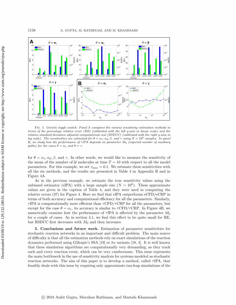
1158 A. GUPTA, M. RATHINAM, AND M. KHAMMASH
Unbiased
𝜃 = 𝛂2 𝜃 = β
𝜃 = 𝛄Unbiased Unbiased
Unbiased
A 𝜃 = 𝛂1
B 𝜃 = 𝛂1 𝜃 = 𝛄
eIPA IPA eCFD CFD eCRP CRP0
2
4
6
8
10
12
RE%
10-3
10-2
10-1
100
RSD
CC
RE%RSDCC
eIPA IPA eCFD CFD eCRP CRP0
5
10
15
20
25
30
RE%
10-4
10-3
10-2
10-1
100
RSD
CC
RE%RSDCC
eIPA IPA eCFD CFD eCRP CRP0
10
20
30
40
50
RE%
10-4
10-3
10-2
10-1
100
RSD
CC
RE%RSDCC
eIPA IPA eCFD CFD eCRP CRP0
2
4
6
8
10
12
RE%
10-4
10-3
10-2
RSD
CC
RE%RSDCC
100 101 102 103M0
0
2
4
6
8
10
RE%
10-4
10-3
10-2
10-1
RSD
CC
RE%RSDCC
100 101 102 103M0
0
5
10
15
20
RE%
10-4
10-3
10-2
RSD
CC
RE%RSDCC
Fig. 4. Genetic toggle switch: Panel A compares the various sensitivity estimation methods interms of the percentage relative error (RE) (calibrated with the left y-axis in linear scale) and therelative standard deviation adjusted computational cost (RSDCC) (calibrated with the right y-axis inlog scale). The sensitivities are estimated for \theta = \alpha 1, \alpha 2, \beta , and \gamma using N = 105 samples. In panelB, we study how the performance of \tau IPA depends on parameter M0 (expected number of auxiliarypaths) for the cases \theta = \alpha 1 and \theta = \gamma .
for \theta = \alpha 1, \alpha 2, \beta , and \gamma . In other words, we would like to measure the sensitivity ofthe mean of the number of \scrU molecules at time T = 10 with respect to all the modelparameters. For this example, we set \tau max = 0.1. We estimate these sensitivities withall the six methods, and the results are presented in Table 4 in Appendix B and inFigure 4A.
As in the previous example, we estimate the true sensitivity values using theunbiased estimator (eIPA) with a large sample size (N = 106). These approximatevalues are given in the caption of Table 4, and they were used in computing therelative errors (37) for Figure 4. Here we find that eIPA outperforms eCFD/eCRP interms of both accuracy and computational efficiency for all the parameters. Similarly,\tau IPA is computationally more efficient than \tau CFD/\tau CRP for all the parameters, butexcept for the case \theta = \alpha 1, its accuracy is similar to \tau CFD/\tau CRP. In Figure 4B, wenumerically examine how the performance of \tau IPA is affected by the parameter M0
for a couple of cases. As in section 4.1, we find this effect to be quite small for RE,but RSDCC first decreases with M0 and then increases.
5. Conclusions and future work. Estimation of parameter sensitivities forstochastic reaction networks in an important and difficult problem. The main sourceof difficulty is that all the estimation methods rely on exact simulations of the reactiondynamics performed using Gillespie's SSA [19] or its variants [18, 4]. It is well knownthat these simulation algorithms are computationally very demanding, as they trackeach and every reaction event, which can be very cumbersome. This issue representsthe main bottleneck in the use of sensitivity analysis for systems modeled as stochasticreaction networks. The aim of this paper is to develop a method, called \tau IPA, thatfeasibly deals with this issue by requiring only approximate tau-leap simulations of the
c\bigcirc 2018 Ankit Gupta, Muruhan Rathinam, and Mustafa Khammash
Dow
nloa
ded
03/0
8/19
to 1
29.1
32.1
80.6
1. R
edis
trib
utio
n su
bjec
t to
SIA
M li
cens
e or
cop
yrig
ht; s
ee h
ttp://
ww
w.s
iam
.org
/jour
nals
/ojs
a.ph
p
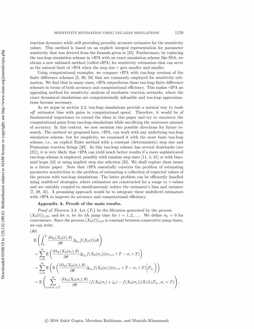
SENSITIVITY ESTIMATION USING TAU-LEAP SIMULATIONS 1159
reaction dynamics while still providing provably accurate estimates for the sensitivityvalues. This method is based on an explicit integral representation for parametersensitivity that was derived from the formula given in [25]. Furthermore, by replacingthe tau-leap simulation scheme in \tau IPA with an exact simulation scheme like SSA, weobtain a new unbiased method (called eIPA) for sensitivity estimation that can serveas the natural limit of \tau IPA when the step size \tau gets smaller and smaller.
Using computational examples, we compare \tau IPA with tau-leap versions of thefinite difference schemes [2, 39, 50] that are commonly employed for sensitivity esti-mation. We find that in many cases, \tau IPA outperforms these tau-leap finite differenceschemes in terms of both accuracy and computational efficiency. This makes \tau IPA anappealing method for sensitivity analysis of stochastic reaction networks, where theexact dynamical simulations are computationally infeasible and tau-leap approxima-tions become necessary.
As we argue in section 2.3, tau-leap simulations provide a natural way to tradeoff estimator bias with gains in computational speed. Therefore, it would be offundamental importance to extend the ideas in this paper and try to maximize thecomputational gains from tau-leap simulations while sacrificing the minimum amountof accuracy. In this context, we now mention two possible directions for future re-search. The method we proposed here, \tau IPA, can work with any underlying tau-leapsimulation scheme, but for simplicity, we examined it with the most basic tau-leapscheme, i.e., an explicit Euler method with a constant (deterministic) step size andPoissonian reaction firings [20]. As this tau-leap scheme has several drawbacks (see[21]), it is very likely that \tau IPA can yield much better results if a more sophisticatedtau-leap scheme is employed, possibly with random step sizes [11, 5, 31] or with bino-mial leaps [42] or using implicit step size selection [35]. We shall explore these issuesin a future paper. Note that \tau IPA essentially converts the problem of estimatingparameter sensitivities to the problem of estimating a collection of expected values ofthe process with tau-leap simulations. The latter problem can be efficiently handledusing multilevel strategies, where estimators are constructed for a range to \tau -valuesand are suitably coupled to simultaneously reduce the estimator's bias and variance[7, 29, 31]. A promising approach would be to integrate these multilevel estimatorswith \tau IPA to improve its accuracy and computational efficiency.
Appendix A. Proofs of the main results.
Proof of Theorem 3.3. Let \{ \scrF t\} be the filtration generated by the process(X\theta (t))t\geq 0, and let \sigma i be its ith jump time for i = 1, 2, . . . . We define \sigma 0 = 0 forconvenience. Since the process (X\theta (t))t\geq 0 is constant between consecutive jump times,we can write
\BbbE
\Biggl( \int T
0
\partial \lambda k(X\theta (t), \theta )
\partial \theta \Delta \zeta kf(X\theta (t))dt
\Biggr) (40)
=
\infty \sum i=0
\BbbE \biggl( \partial \lambda k(X\theta (\sigma i), \theta )
\partial \theta \Delta \zeta kf(X\theta (\sigma i))(\sigma i+1 \wedge T - \sigma i \wedge T )
\biggr)
=
\infty \sum i=0
\BbbE \biggl( \BbbE \biggl( \partial \lambda k(X\theta (\sigma i), \theta )
\partial \theta \Delta \zeta kf(X\theta (\sigma i))(\sigma i+1 \wedge T - \sigma i \wedge T )
\bigm| \bigm| \bigm| \bigm| \scrF \sigma i
\biggr) \biggr)
= \BbbE
\Biggl( \infty \sum i=0:\sigma i<T
\partial \lambda k(X\theta (\sigma i), \theta )
\partial \theta (f(X\theta (\sigma i) + \zeta k) - f(X\theta (\sigma i)))\BbbE (\delta i| \scrF \sigma i
, \sigma i < T )
\Biggr) ,
c\bigcirc 2018 Ankit Gupta, Muruhan Rathinam, and Mustafa Khammash
Dow
nloa
ded
03/0
8/19
to 1
29.1
32.1
80.6
1. R
edis
trib
utio
n su
bjec
t to
SIA
M li
cens
e or
cop
yrig
ht; s
ee h
ttp://
ww
w.s
iam
.org
/jour
nals
/ojs
a.ph
p
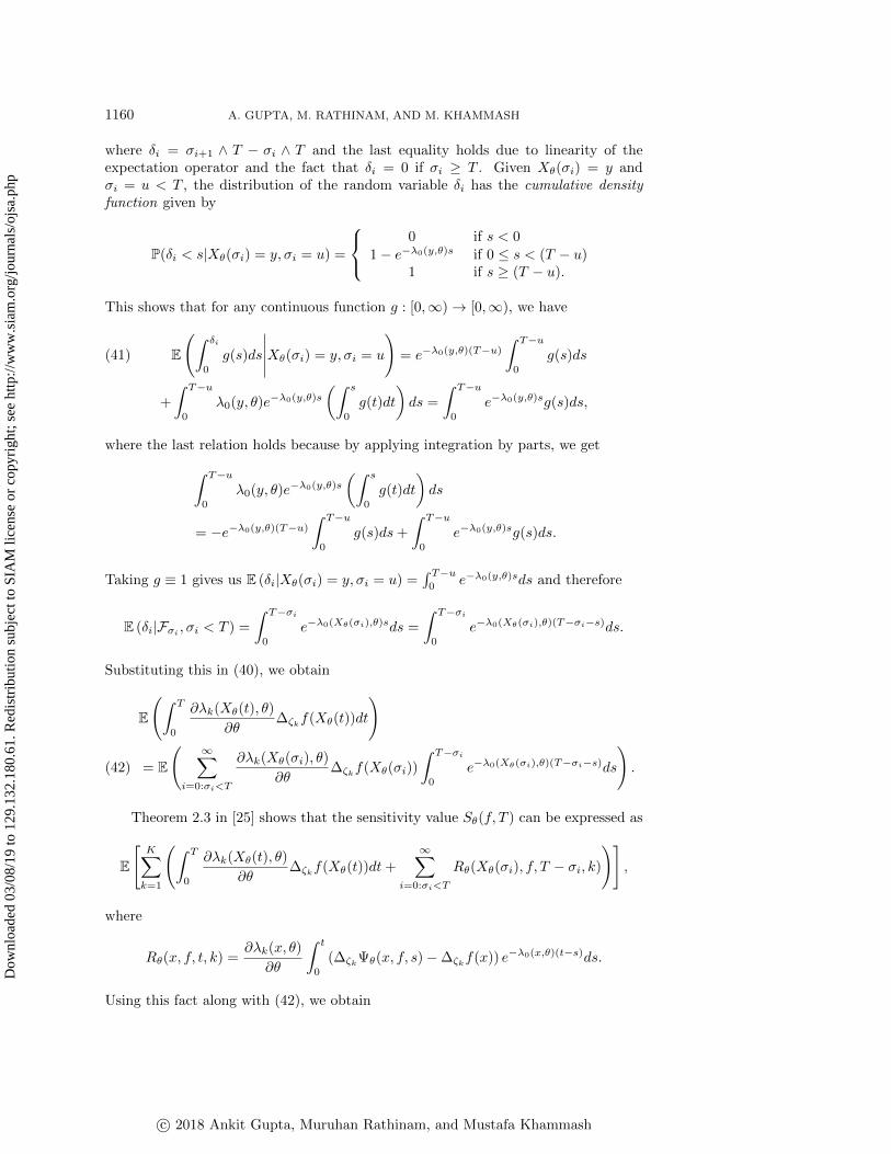
1160 A. GUPTA, M. RATHINAM, AND M. KHAMMASH
where \delta i = \sigma i+1 \wedge T - \sigma i \wedge T and the last equality holds due to linearity of theexpectation operator and the fact that \delta i = 0 if \sigma i \geq T . Given X\theta (\sigma i) = y and\sigma i = u < T , the distribution of the random variable \delta i has the cumulative densityfunction given by
\BbbP (\delta i < s| X\theta (\sigma i) = y, \sigma i = u) =
\left\{ 0 if s < 0
1 - e - \lambda 0(y,\theta )s if 0 \leq s < (T - u)1 if s \geq (T - u).
This shows that for any continuous function g : [0,\infty )\rightarrow [0,\infty ), we have
\BbbE
\Biggl( \int \delta i
0
g(s)ds
\bigm| \bigm| \bigm| \bigm| \bigm| X\theta (\sigma i) = y, \sigma i = u
\Biggr) = e - \lambda 0(y,\theta )(T - u)
\int T - u
0
g(s)ds(41)
+
\int T - u
0
\lambda 0(y, \theta )e - \lambda 0(y,\theta )s
\biggl( \int s
0
g(t)dt
\biggr) ds =
\int T - u
0
e - \lambda 0(y,\theta )sg(s)ds,
where the last relation holds because by applying integration by parts, we get\int T - u
0
\lambda 0(y, \theta )e - \lambda 0(y,\theta )s
\biggl( \int s
0
g(t)dt
\biggr) ds
= - e - \lambda 0(y,\theta )(T - u)
\int T - u
0
g(s)ds+
\int T - u
0
e - \lambda 0(y,\theta )sg(s)ds.
Taking g \equiv 1 gives us \BbbE (\delta i| X\theta (\sigma i) = y, \sigma i = u) =\int T - u
0e - \lambda 0(y,\theta )sds and therefore
\BbbE (\delta i| \scrF \sigma i , \sigma i < T ) =
\int T - \sigma i
0
e - \lambda 0(X\theta (\sigma i),\theta )sds =
\int T - \sigma i
0
e - \lambda 0(X\theta (\sigma i),\theta )(T - \sigma i - s)ds.
Substituting this in (40), we obtain
\BbbE
\Biggl( \int T
0
\partial \lambda k(X\theta (t), \theta )
\partial \theta \Delta \zeta kf(X\theta (t))dt
\Biggr)
= \BbbE
\Biggl( \infty \sum i=0:\sigma i<T
\partial \lambda k(X\theta (\sigma i), \theta )
\partial \theta \Delta \zeta kf(X\theta (\sigma i))
\int T - \sigma i
0
e - \lambda 0(X\theta (\sigma i),\theta )(T - \sigma i - s)ds
\Biggr) .(42)
Theorem 2.3 in [25] shows that the sensitivity value S\theta (f, T ) can be expressed as
\BbbE
\Biggl[ K\sum
k=1
\Biggl( \int T
0
\partial \lambda k(X\theta (t), \theta )
\partial \theta \Delta \zeta kf(X\theta (t))dt+
\infty \sum i=0:\sigma i<T
R\theta (X\theta (\sigma i), f, T - \sigma i, k)
\Biggr) \Biggr] ,
where
R\theta (x, f, t, k) =\partial \lambda k(x, \theta )
\partial \theta
\int t
0
(\Delta \zeta k\Psi \theta (x, f, s) - \Delta \zeta kf(x)) e - \lambda 0(x,\theta )(t - s)ds.
Using this fact along with (42), we obtain
c\bigcirc 2018 Ankit Gupta, Muruhan Rathinam, and Mustafa Khammash
Dow
nloa
ded
03/0
8/19
to 1
29.1
32.1
80.6
1. R
edis
trib
utio
n su
bjec
t to
SIA
M li
cens
e or
cop
yrig
ht; s
ee h
ttp://
ww
w.s
iam
.org
/jour
nals
/ojs
a.ph
p
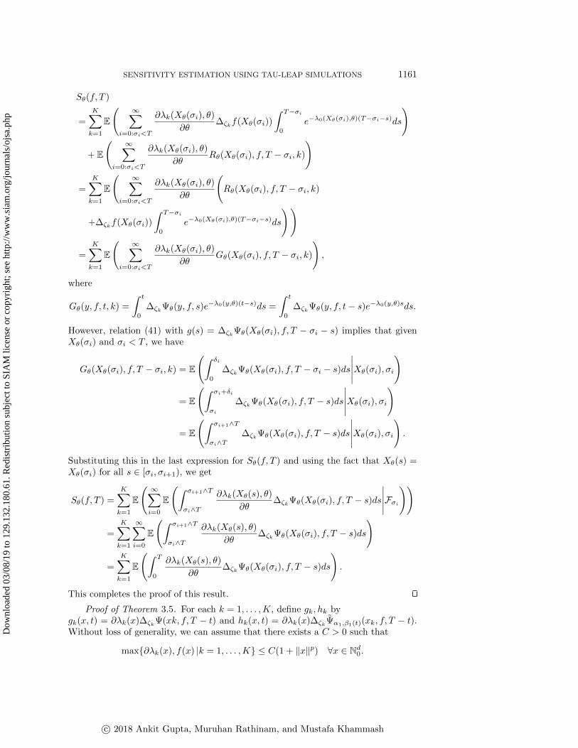
SENSITIVITY ESTIMATION USING TAU-LEAP SIMULATIONS 1161
S\theta (f, T )
=
K\sum k=1
\BbbE
\Biggl( \infty \sum i=0:\sigma i<T
\partial \lambda k(X\theta (\sigma i), \theta )
\partial \theta \Delta \zeta kf(X\theta (\sigma i))
\int T - \sigma i
0
e - \lambda 0(X\theta (\sigma i),\theta )(T - \sigma i - s)ds
\Biggr)
+ \BbbE
\Biggl( \infty \sum i=0:\sigma i<T
\partial \lambda k(X\theta (\sigma i), \theta )
\partial \theta R\theta (X\theta (\sigma i), f, T - \sigma i, k)
\Biggr)
=
K\sum k=1
\BbbE
\Biggl( \infty \sum i=0:\sigma i<T
\partial \lambda k(X\theta (\sigma i), \theta )
\partial \theta
\Biggl( R\theta (X\theta (\sigma i), f, T - \sigma i, k)
+\Delta \zeta kf(X\theta (\sigma i))
\int T - \sigma i
0
e - \lambda 0(X\theta (\sigma i),\theta )(T - \sigma i - s)ds
\Biggr) \Biggr)
=
K\sum k=1
\BbbE
\Biggl( \infty \sum i=0:\sigma i<T
\partial \lambda k(X\theta (\sigma i), \theta )
\partial \theta G\theta (X\theta (\sigma i), f, T - \sigma i, k)
\Biggr) ,
where
G\theta (y, f, t, k) =
\int t
0
\Delta \zeta k\Psi \theta (y, f, s)e - \lambda 0(y,\theta )(t - s)ds =
\int t
0
\Delta \zeta k\Psi \theta (y, f, t - s)e - \lambda 0(y,\theta )sds.
However, relation (41) with g(s) = \Delta \zeta k\Psi \theta (X\theta (\sigma i), f, T - \sigma i - s) implies that givenX\theta (\sigma i) and \sigma i < T , we have
G\theta (X\theta (\sigma i), f, T - \sigma i, k) = \BbbE
\Biggl( \int \delta i
0
\Delta \zeta k\Psi \theta (X\theta (\sigma i), f, T - \sigma i - s)ds
\bigm| \bigm| \bigm| \bigm| \bigm| X\theta (\sigma i), \sigma i
\Biggr)
= \BbbE
\Biggl( \int \sigma i+\delta i
\sigma i
\Delta \zeta k\Psi \theta (X\theta (\sigma i), f, T - s)ds
\bigm| \bigm| \bigm| \bigm| \bigm| X\theta (\sigma i), \sigma i
\Biggr)
= \BbbE
\Biggl( \int \sigma i+1\wedge T
\sigma i\wedge T
\Delta \zeta k\Psi \theta (X\theta (\sigma i), f, T - s)ds
\bigm| \bigm| \bigm| \bigm| \bigm| X\theta (\sigma i), \sigma i
\Biggr) .
Substituting this in the last expression for S\theta (f, T ) and using the fact that X\theta (s) =X\theta (\sigma i) for all s \in [\sigma i, \sigma i+1), we get
S\theta (f, T ) =
K\sum k=1
\BbbE
\Biggl( \infty \sum i=0
\BbbE
\Biggl( \int \sigma i+1\wedge T
\sigma i\wedge T
\partial \lambda k(X\theta (s), \theta )
\partial \theta \Delta \zeta k\Psi \theta (X\theta (\sigma i), f, T - s)ds
\bigm| \bigm| \bigm| \bigm| \bigm| \scrF \sigma i
\Biggr) \Biggr)
=
K\sum k=1
\infty \sum i=0
\BbbE
\Biggl( \int \sigma i+1\wedge T
\sigma i\wedge T
\partial \lambda k(X\theta (s), \theta )
\partial \theta \Delta \zeta k\Psi \theta (X\theta (\sigma i), f, T - s)ds
\Biggr)
=
K\sum k=1
\BbbE
\Biggl( \int T
0
\partial \lambda k(X\theta (s), \theta )
\partial \theta \Delta \zeta k\Psi \theta (X\theta (\sigma i), f, T - s)ds
\Biggr) .
This completes the proof of this result.
Proof of Theorem 3.5. For each k = 1, . . . ,K, define gk, hk bygk(x, t) = \partial \lambda k(x)\Delta \zeta k\Psi (xk, f, T - t) and hk(x, t) = \partial \lambda k(x)\Delta \zeta k
\~\Psi \alpha 1,\beta 1(t)(xk, f, T - t).Without loss of generality, we can assume that there exists a C > 0 such that
max\{ \partial \lambda k(x), f(x) | k = 1, . . . ,K\} \leq C(1 + \| x\| p) \forall x \in \BbbN d0.
c\bigcirc 2018 Ankit Gupta, Muruhan Rathinam, and Mustafa Khammash
Dow
nloa
ded
03/0
8/19
to 1
29.1
32.1
80.6
1. R
edis
trib
utio
n su
bjec
t to
SIA
M li
cens
e or
cop
yrig
ht; s
ee h
ttp://
ww
w.s
iam
.org
/jour
nals
/ojs
a.ph
p

1162 A. GUPTA, M. RATHINAM, AND M. KHAMMASH
Then, due to Lemma 3.2, we obtain
(43)
supt\in [0,T ]
| hk(x, t) - gk(x, t)|
\leq \partial \lambda k(x)CC1(p, T, \alpha 1)\Bigl( (1 + \| x\| \xi (p)) + (1 + \| x+ \zeta k\| \xi (p))
\Bigr) \tau \gamma max
\leq C2C1(p, T, \alpha 1)(1 + \| x\| p)\Bigl( (1 + \| x\| \xi (p)) + (1 + \| x+ \zeta k\| \xi (p))
\Bigr) \tau \gamma max
\leq c0(p)C2C1(p, T, \alpha 1)
\Bigl( 1 + \| x\| (p+\xi (p))
\Bigr) \tau \gamma max,
where c0(p) is a constant that depends only on p as well as \zeta 1, . . . , \zeta K . Lemma 3.2also shows that
(44)sup
t\in [0,T ]
| hk(x, t)| \leq \partial \lambda k(x)CC3(p, T, \alpha 1) ((1 + \| x\| p) + (1 + \| x+ \zeta k\| p))
\leq c1(p)C2C3(p, T, \alpha 1)(1 + \| x\| 2p)
and supt\in [0,T ] | gk(x, t)| \leq c1(p)C2C2(p, T )(1+ \| x\| 2p), where c1(p) is again a constant
that depends only on p and \zeta 1, . . . , \zeta K .From (44) and Lemma 3.2, it follows that
supt\in [0,T ]
| \BbbE (hk(Z\alpha 0,\beta 0(x0, t), t)) - \BbbE (hk(X(t), t))| (45)
\leq c1(p)C2C3(p, T, \alpha 1)C1(2p, T, \alpha 0)
\Bigl( 1 + \| x0\| \xi (2p)
\Bigr) \tau \gamma max.
Moreover, from (43), we get
\BbbE (| hk(X(t), t) - gk(X(t), t)| ) \leq c0(p)C2C1(p, T, \alpha 1)(1 + \BbbE (\| X(t)\| (p+\xi (p))))\tau \gamma max,
and hence using Assumption 2, we obtain
supt\in [0,T ]
\BbbE (| hk(X(t), t) - gk(X(t), t)| )(46)
\leq c0(p)C2C1(p, T, \alpha 1)C2(p+ \xi (p), T )
\Bigl( 1 + \| x0\| p+\xi (p)
\Bigr) \tau \gamma max.
Note that\bigm| \bigm| \bigm| \~S(f, T ) - S(f, T )\bigm| \bigm| \bigm| = \bigm| \bigm| \bigm| \bigm| \bigm|
K\sum k=1
\int T
0
(\BbbE (hk(Z\alpha 0,\beta 0(x0, t), t)) - \BbbE (gk(X(t), t))) dt
\bigm| \bigm| \bigm| \bigm| \bigm| \leq
K\sum k=1
\bigm| \bigm| \bigm| \int T
0
\BbbE (hk(Z\alpha 0,\beta 0(x0, t), t))dt -
\int T
0
\BbbE (gk(X(t), t))dt\bigm| \bigm| \bigm|
\leq K\sum
k=1
\int T
0
| \BbbE (hk(Z\alpha 0,\beta 0(x0, t), t)) - \BbbE (hk(X(t), t))| dt
+
K\sum k=1
\int T
0
| \BbbE (hk(X(t), t)) - \BbbE (gk(X(t), t))| dt.
Using (45) and (46), we obtain the bound
c\bigcirc 2018 Ankit Gupta, Muruhan Rathinam, and Mustafa Khammash
Dow
nloa
ded
03/0
8/19
to 1
29.1
32.1
80.6
1. R
edis
trib
utio
n su
bjec
t to
SIA
M li
cens
e or
cop
yrig
ht; s
ee h
ttp://
ww
w.s
iam
.org
/jour
nals
/ojs
a.ph
p

SENSITIVITY ESTIMATION USING TAU-LEAP SIMULATIONS 1163\bigm| \bigm| \bigm| \~S(f, T ) - S(f, T )\bigm| \bigm| \bigm| \leq KTc1(p)C
2C3(p, T, \alpha 1)C1(2p, T, \alpha 0)\Bigl( 1 + \| x0\| \xi (2p)
\Bigr) \tau \gamma max
+KTc0(p)C2C1(p, T, \alpha 1)C2(p+ \xi (p), T )
\Bigl( 1 + \| x0\| p+\xi (p)
\Bigr) \tau \gamma max,
which proves the theorem.
Appendix B. Supplementary tables and algorithms.
Table 3Birth-death model: Sensitivity estimation results for T = 5, 10. For all the methods, N = 105
are used to estimate the following quantities---the estimator mean (6), the standard deviation (9),the relative error (RE) percentage (37), and the relative standard deviation adjusted computationcost (RSDCC) (38) in seconds. The exact sensitivity values are - 90.204 for T = 5 and - 264.241for T = 10.
eIPA \tau IPAT Mean Std Dev RE\% RSDCC Mean Std Dev RE\% RSDCC
5 -90.079 0.093 0.139 0.379E-5 -90.938 0.078 0.813 0.121E-510 -264.5 0.309 0.099 0.97E-5 -266.34 0.243 0.793 0.247E-5
eCFD \tau CFDT Mean Std Dev RE\% RSDCC Mean Std Dev RE\% RSDCC
5 -90.632 0.088 0.4746 0.078E-5 -86.456 0.089 4.155 0.033E-510 -268.77 0.142 1.716 0.054E-5 -268.214 0.146 1.503 0.021E-5
eCRP \tau CRPT Mean Std Dev RE\% RSDCC Mean Std Dev RE\% RSDCC
5 -90.749 0.097 0.604 0.343E-5 -86.481 0.098 4.128 0.343E-510 -268.82 0.169 1.734 0.152E-5 -267.92 0.173 1.393 0.131E-5
Table 4Genetic toggle switch: Sensitivity estimation results w.r.t. all the model parameters \alpha 1, \alpha 2, \beta ,
and \gamma . For all the methods, N = 105 are used to estimate the following quantities---the estimatormean (6), the standard deviation (9), the relative error (RE) percentage (37), and the relativestandard deviation adjusted computation cost (RSDCC) (38) in seconds. The true sensitivity valuesare approximately 1.195\pm 0.009 for \theta = \alpha 1, - 2.1194\pm 0.01 for \theta = \alpha 2, - 5.9929\pm 0.035 for \theta = \beta ,and 54.5721 \pm 0.133 for \theta = \gamma . These values are estimated with eIPA using 106 samples, and theyare expressed in the form s0 \pm l, which signifies that the 99\% confidence interval is (s0 - l, s0 + l).
eIPA \tau IPA\theta Mean Std Dev RE\% RSDCC Mean Std Dev RE\% RSDCC
\alpha 1 1.202 0.0107 0.625 0.0046 1.185 0.0131 0.822 0.0023\alpha 2 -2.133 0.0132 0.663 0.0021 -2.3968 0.0148 13.087 0.0008\beta -5.924 0.0419 1.144 0.0020 -8.5372 0.0562 42.456 0.0008\gamma 54.372 0.1679 0.367 0.0009 60.156 0.191 10.232 0.0003
eCFD \tau CFD\theta Mean Std Dev RE\% RSDCC Mean Std Dev RE\% RSDCC
\alpha 1 1.053 0.11 11.883 0.1925 1.183 0.0491 1.021 0.0088\alpha 2 -2.007 0.267 5.305 0.3219 -2.734 0.0991 29.011 0.0066\beta -5.865 0.4535 2.1339 0.1053 -8.787 0.1813 46.617 0.0021\gamma 54.67 1.1589 0.1794 0.0080 59.431 0.3907 8.9044 0.0002
eCRP \tau CRP\theta Mean Std Dev RE\% RSDCC Mean Std Dev RE\% RSDCC
\alpha 1 1.158 0.0793 3.13 0.0919 1.129 0.0781 5.4895 0.0562\alpha 2 -1.999 0.1306 5.701 0.0823 -2.415 0.1109 13.9646 0.0254\beta -6.21 0.1777 3.625 0.0161 -8.853 0.2198 47.7203 0.0074\gamma 54.546 0.4756 0.0469 0.0015 59.807 0.4267 9.5925 0.0006
c\bigcirc 2018 Ankit Gupta, Muruhan Rathinam, and Mustafa Khammash
Dow
nloa
ded
03/0
8/19
to 1
29.1
32.1
80.6
1. R
edis
trib
utio
n su
bjec
t to
SIA
M li
cens
e or
cop
yrig
ht; s
ee h
ttp://
ww
w.s
iam
.org
/jour
nals
/ojs
a.ph
p
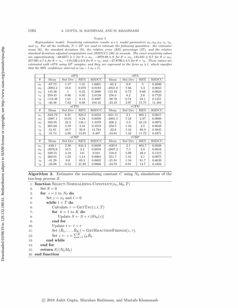
1164 A. GUPTA, M. RATHINAM, AND M. KHAMMASH
Table 5Repressilator model: Sensitivity estimation results w.r.t. model parameters \alpha 1, \alpha 2, \alpha 3, \gamma 1, \gamma 2,
and \gamma 3. For all the methods, N = 105 are used to estimate the following quantities---the estimatormean (6), the standard deviation (9), the relative error (RE) percentage (37), and the relativestandard deviation adjusted computation cost (RSDCC) (38) in seconds. The exact sensitivity valuesare approximately - 68.6271 \pm 1 for \theta = \alpha 1, - 2979.88 \pm 8 for \theta = \alpha 2, 145.041 \pm 0.7 for \theta = \alpha 3,257.091\pm 7.4 for \theta = \gamma 1, - 119.526\pm 0.9 for \theta = \gamma 2, and - 27.8796\pm 4.5 for \theta = \gamma 3. These values areestimated with eIPA using 106 samples, and they are expressed in the form s0 \pm l, which signifiesthat the 99\% confidence interval is (s0 - l, s0 + l).
eIPA \tau IPA\theta Mean Std Dev RE\% RSDCC Mean Std Dev RE\% RSDCC
\alpha 1 -67.73 1.17 1.31 1.6801 -65.2 0.8 5 0.2886\alpha 2 -2982.2 10.6 0.078 0.0193 -2821.8 7.66 5.3 0.0053\alpha 3 145.36 1 0.22 0.2880 131.04 0.73 9.66 0.0623\gamma 1 259.45 8.86 0.92 2.0139 250.4 8.2 2.6 0.7723\gamma 2 -119.38 1.01 0.13 0.4097 -90.78 0.74 24.1 0.1251\gamma 3 -30.38 7.82 8.98 104.45 -23.45 2.97 15.75 11.484
eCFD \tau CFD\theta Mean Std Dev RE\% RSDCC Mean Std Dev RE\% RSDCC
\alpha 1 -633.79 6.21 823.5 0.0334 -621.15 2.1 805.1 0.0017\alpha 2 -2987.1 10.01 0.24 0.0039 -2891.5 7.16 2.97 0.0009\alpha 3 356.95 22.3 146.1 1.3379 206.2 5.3 42.19 0.0972\gamma 1 265.69 4.59 3.34 0.1019 250.5 1.43 2.5 0.0048\gamma 2 -51.61 10.7 56.8 14.764 -22.8 1.16 80.9 0.3845\gamma 3 -31.74 4.98 13.85 8.407 -24.61 1.42 11.72 0.4871
eCRP \tau CRP\theta Mean Std Dev RE\% RSDCC Mean Std Dev RE\% RSDCC
\alpha 1 -648.1 2.38 844.3 0.0039 -620.9 2.1 804.7 0.0028\alpha 2 -3076.6 10.5 3.2 0.0033 -2897.2 7.5 2.8 0.0016\alpha 3 349.55 4.18 141 0.041 216.6 5.09 49.4 0.1315\gamma 1 260.01 1.23 1.14 0.0064 251.7 1.41 2.1 0.0075\gamma 2 -41.29 0.6 65.5 0.0602 -21.91 1.16 81.7 0.6639\gamma 3 -33.98 0.52 21.88 0.0666 -23.78 0.91 14.7 0.3494
Algorithm 2. Estimates the normalizing constant C using N0 simulations of thetau-leap process Z.
1: function Select-Normalizing-Constant(x0,M0, T )2: Set S = 03: for i = 1 to N0 do4: Set z = x0 and t = 05: while t < T do6: Calculate \tau = GetTau(z, t, T )7: for k = 1 to K do8: Update S \leftarrow S + \tau | \partial \lambda k(z)| 9: end for
10: Update t\leftarrow t+ \tau 11: Set ( \~R1, . . . , \~RK) = GetReactionFirings(z, \tau ).
12: Set z \leftarrow z +\sum K
k=1 \zeta k\~Rk.
13: end while14: end for15: return S/(N0M0)16: end function
c\bigcirc 2018 Ankit Gupta, Muruhan Rathinam, and Mustafa Khammash
Dow
nloa
ded
03/0
8/19
to 1
29.1
32.1
80.6
1. R
edis
trib
utio
n su
bjec
t to
SIA
M li
cens
e or
cop
yrig
ht; s
ee h
ttp://
ww
w.s
iam
.org
/jour
nals
/ojs
a.ph
p
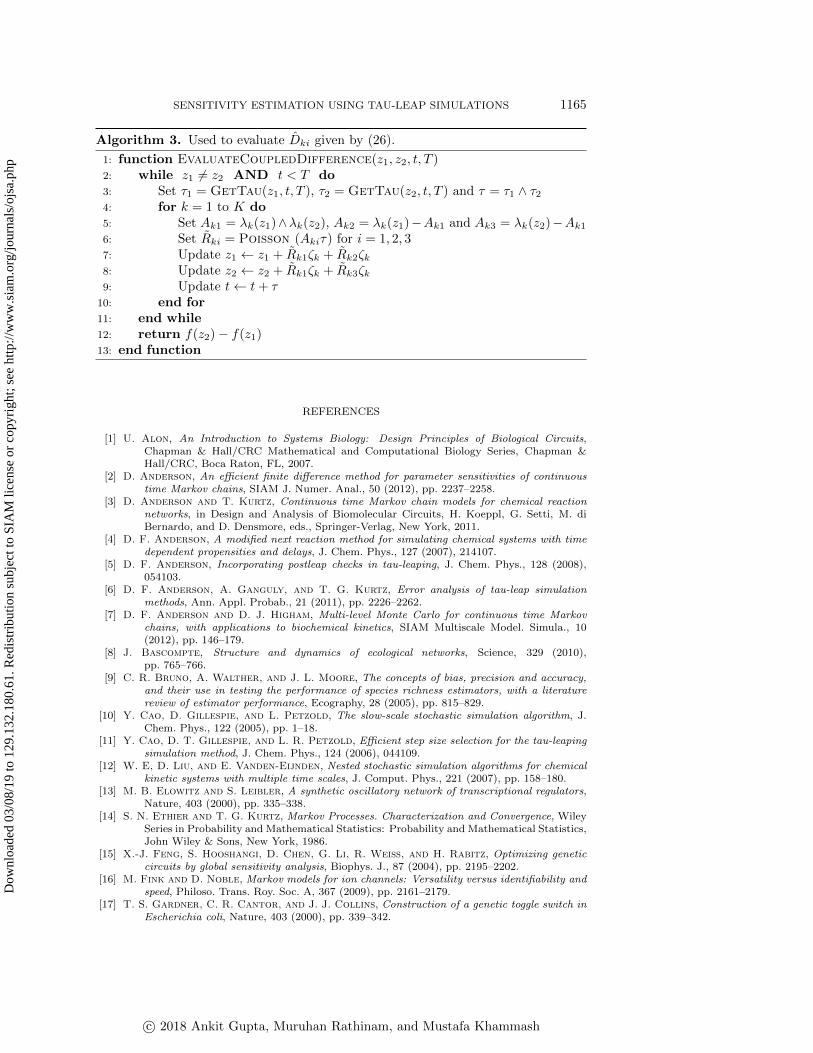
SENSITIVITY ESTIMATION USING TAU-LEAP SIMULATIONS 1165
Algorithm 3. Used to evaluate \^Dki given by (26).
1: function EvaluateCoupledDifference(z1, z2, t, T )2: while z1 \not = z2 AND t < T do3: Set \tau 1 = GetTau(z1, t, T ), \tau 2 = GetTau(z2, t, T ) and \tau = \tau 1 \wedge \tau 24: for k = 1 to K do5: Set Ak1 = \lambda k(z1)\wedge \lambda k(z2), Ak2 = \lambda k(z1) - Ak1 and Ak3 = \lambda k(z2) - Ak1
6: Set \~Rki = Poisson (Aki\tau ) for i = 1, 2, 37: Update z1 \leftarrow z1 + \~Rk1\zeta k + \~Rk2\zeta k8: Update z2 \leftarrow z2 + \~Rk1\zeta k + \~Rk3\zeta k9: Update t\leftarrow t+ \tau
10: end for11: end while12: return f(z2) - f(z1)13: end function
REFERENCES
[1] U. Alon, An Introduction to Systems Biology: Design Principles of Biological Circuits,Chapman \& Hall/CRC Mathematical and Computational Biology Series, Chapman \&Hall/CRC, Boca Raton, FL, 2007.
[2] D. Anderson, An efficient finite difference method for parameter sensitivities of continuoustime Markov chains, SIAM J. Numer. Anal., 50 (2012), pp. 2237--2258.
[3] D. Anderson and T. Kurtz, Continuous time Markov chain models for chemical reactionnetworks, in Design and Analysis of Biomolecular Circuits, H. Koeppl, G. Setti, M. diBernardo, and D. Densmore, eds., Springer-Verlag, New York, 2011.
[4] D. F. Anderson, A modified next reaction method for simulating chemical systems with timedependent propensities and delays, J. Chem. Phys., 127 (2007), 214107.
[5] D. F. Anderson, Incorporating postleap checks in tau-leaping, J. Chem. Phys., 128 (2008),054103.
[6] D. F. Anderson, A. Ganguly, and T. G. Kurtz, Error analysis of tau-leap simulationmethods, Ann. Appl. Probab., 21 (2011), pp. 2226--2262.
[7] D. F. Anderson and D. J. Higham, Multi-level Monte Carlo for continuous time Markovchains, with applications to biochemical kinetics, SIAM Multiscale Model. Simula., 10(2012), pp. 146--179.
[8] J. Bascompte, Structure and dynamics of ecological networks, Science, 329 (2010),pp. 765--766.
[9] C. R. Bruno, A. Walther, and J. L. Moore, The concepts of bias, precision and accuracy,and their use in testing the performance of species richness estimators, with a literaturereview of estimator performance, Ecography, 28 (2005), pp. 815--829.
[10] Y. Cao, D. Gillespie, and L. Petzold, The slow-scale stochastic simulation algorithm, J.Chem. Phys., 122 (2005), pp. 1--18.
[11] Y. Cao, D. T. Gillespie, and L. R. Petzold, Efficient step size selection for the tau-leapingsimulation method, J. Chem. Phys., 124 (2006), 044109.
[12] W. E, D. Liu, and E. Vanden-Eijnden, Nested stochastic simulation algorithms for chemicalkinetic systems with multiple time scales, J. Comput. Phys., 221 (2007), pp. 158--180.
[13] M. B. Elowitz and S. Leibler, A synthetic oscillatory network of transcriptional regulators,Nature, 403 (2000), pp. 335--338.
[14] S. N. Ethier and T. G. Kurtz, Markov Processes. Characterization and Convergence, WileySeries in Probability and Mathematical Statistics: Probability and Mathematical Statistics,John Wiley \& Sons, New York, 1986.
[15] X.-J. Feng, S. Hooshangi, D. Chen, G. Li, R. Weiss, and H. Rabitz, Optimizing geneticcircuits by global sensitivity analysis, Biophys. J., 87 (2004), pp. 2195--2202.
[16] M. Fink and D. Noble, Markov models for ion channels: Versatility versus identifiability andspeed, Philoso. Trans. Roy. Soc. A, 367 (2009), pp. 2161--2179.
[17] T. S. Gardner, C. R. Cantor, and J. J. Collins, Construction of a genetic toggle switch inEscherichia coli, Nature, 403 (2000), pp. 339--342.
c\bigcirc 2018 Ankit Gupta, Muruhan Rathinam, and Mustafa Khammash
Dow
nloa
ded
03/0
8/19
to 1
29.1
32.1
80.6
1. R
edis
trib
utio
n su
bjec
t to
SIA
M li
cens
e or
cop
yrig
ht; s
ee h
ttp://
ww
w.s
iam
.org
/jour
nals
/ojs
a.ph
p
1166 A. GUPTA, M. RATHINAM, AND M. KHAMMASH
[18] M. A. Gibson and J. Bruck, Efficient exact stochastic simulation of chemical systems withmany species and many channels, J. Phys. Chem. A, 104 (2000), pp. 1876--1889.
[19] D. T. Gillespie, Exact stochastic simulation of coupled chemical reactions, J. Phys. Chem.,81 (1977), pp. 2340--2361.
[20] D. T. Gillespie, Approximate accelerated stochastic simulation of chemically reacting systems,J. Chem. Phys., 115 (2001), pp. 1716--1733.
[21] D. T. Gillespie, Stochastic simulation of chemical kinetics, Annu. Revi. Phys. Chem., 58(2007), pp. 35--55.
[22] P. W. Glynn, Likelihood ratio gradient estimation for stochastic systems, Commun. ACM, 33(1990), pp. 75--84.
[23] R. Gunawan, Y. Cao, and F. Doyle, Sensitivity analysis of discrete stochastic systems,Biophys. J., 88 (2005), pp. 2530--2540.
[24] A. Gupta, C. Briat, and M. Khammash, A scalable computational framework for establish-ing long-term behavior of stochastic reaction networks, PLoS Comput. Biol., 10 (2014),e1003669.
[25] A. Gupta and M. Khammash, Unbiased estimation of parameter sensitivities for stochasticchemical reaction networks, SIAM J. Sci. Comput., 35 (2013), pp. A2598--A2620.
[26] A. Gupta and M. Khammash, An efficient and unbiased method for sensitivity analysis ofstochastic reaction networks, J. Roy. Soci. Interface, 11 (2014), 20140979.
[27] H. Hethcote, The mathematics of infectious diseases, SIAM Rev., 42 (2000), pp. 599--653.[28] J. Karlsson and R. Tempone, Towards automatic global error control: Computable weak
error expansion for the tau-leap method, Monte Carlo Methods Appl., 17 (2011),pp. 233--278.
[29] C. Lester, C. A. Yates, M. B. Giles, and R. E. Baker, An adaptive multi-level simulationalgorithm for stochastic biological systems, J. Chem. Phys., 142 (2015), 024113.
[30] T. Li, Analysis of explicit tau-leaping schemes for simulating chemically reacting systems,Multiscale Model. Simul., 6 (2007), pp. 417--436.
[31] A. Moraes, R. Tempone, and P. Vilanova, Hybrid Chernoff tau-leap, Multiscale Model.Simul., 12 (2014), pp. 581--615.
[32] S. Plyasunov and A. Arkin, Efficient stochastic sensitivity analysis of discrete event systems,J. Comput. Phys., 221 (2007), pp. 724--738.
[33] M. Rathinam, Moment growth bounds on continuous time Markov processes on non-negativeinteger lattices, Quart. Appl. Math., 73 (2015), pp. 347--364.
[34] M. Rathinam, Convergence of moments of tau leaping schemes for unbounded Markov pro-cesses on integer lattices, SIAM J. Numer. Anal., 54 (2016), pp. 415--439.
[35] M. Rathinam, L. R. Petzold, Y. Cao, and D. T. Gillespie, Stiffness in stochastic chem-ically reacting systems: The implicit tau-leaping method, J. Chem. Phys., 119 (2003),pp. 12784--12794.
[36] Y. Cao, L. R. Petzold, M. Rathinam, and D. T. Gillespie, The numerical stability ofleaping methods for stochastic simulation of chemically reacting systems, J. Chem. Phys.,121 (2004), pp. 12169--12178.
[37] M. Rathinam, L. R. Petzold, Y. Cao, and D. T. Gillespie, Consistency and stability oftau-leaping schemes for chemical reaction systems, Multiscale Model. Simul., 4 (2005),pp. 867--895.
[38] M. Rathinam and H. El Samad, Reversible-equivalent-monomolecular tau: A leaping methodfor ``small number and stiff"" stochastic chemical systems, J. Comput. Phys., 224 (2007),pp. 897--923.
[39] M. Rathinam, P. W. Sheppard, and M. Khammash, Efficient computation of parametersensitivities of discrete stochastic chemical reaction networks, J. Chem. Phys., 132 (2010),034103.
[40] P. W. Sheppard, M. Rathinam, and M. Khammash, A pathwise derivative approach to thecomputation of parameter sensitivities in discrete stochastic chemical systems, J. Chem.Phys., 136 (2012), 034115.
[41] J. Stelling, E. D. Gilles, and F. J. Doyle, Robustness properties of circadian clock archi-tectures, Proc. Natl. Acad. Sci. USA, 101 (2004), pp. 13210--13215.
[42] T. Tian and K. Burrage, Binomial leap methods for simulating stochastic chemical kinetics,J. Chem. Phys., 121 (2004), pp. 10356--10364.
[43] J. M. G. Vilar, H. Y. Kueh, N. Barkai, and S. Leibler, Mechanisms of noise-resistance ingenetic oscillator, Proc. Natl. Acad. Sci., 99 (2002), pp. 5988--5992.
[44] T. Wang and M. Rathinam, Efficiency of the Girsanov Transformation Approach for Para-metric Sensitivity Analysis of Stochastic Chemical Kinetics, preprint, arXiv:1412.1005,2016.
c\bigcirc 2018 Ankit Gupta, Muruhan Rathinam, and Mustafa Khammash
Dow
nloa
ded
03/0
8/19
to 1
29.1
32.1
80.6
1. R
edis
trib
utio
n su
bjec
t to
SIA
M li
cens
e or
cop
yrig
ht; s
ee h
ttp://
ww
w.s
iam
.org
/jour
nals
/ojs
a.ph
p
SENSITIVITY ESTIMATION USING TAU-LEAP SIMULATIONS 1167
[45] E. Weinan, D. Liu, and E. Vanden-Eijnden, Nested stochastic simulation algorithm forchemical kinetic systems with disparate rates, J. Chem. Phys., 123 (2005), pp. 1--8.
[46] Y. Yang and M. Rathinam, Tau leaping of stiff stochastic chemical systems via local centrallimit approximation, J. Comput. Phys., 242 (2013), pp. 581--606.
[47] Y. Yang, M. Rathinam, and J. Shen, Integral tau methods for stiff stochastic chemical sys-tems, J. Chem. Phys., 134 (2011), 044129.
[48] T. Li, A. Abdulle, and W. E, Effectiveness of implicit methods for stiff stochastic differentialequations, Commun. Comput. Phys., 3 (2008), pp. 295--307.
[49] I. Cipcigan and M. Rathinam, Uniform convergence of interlaced Euler method for stiffstochastic differential equations, Multiscale Model. Simul., 9 (2011), pp. 1217--1252.
[50] M. Morshed, B. Ingalls, and S. Ilie, An efficient finite-difference strategy for sensitivityanalysis of stochastic models of biochemical systems, Biosystems, 151 (2017), pp. 43--52.
[51] P. B. Warren and R. J. Allen, Steady-state parameter sensitivity in stochastic modeling viatrajectory reweighting, J. Chem. Phys., 136 (2012), 03B603.
c\bigcirc 2018 Ankit Gupta, Muruhan Rathinam, and Mustafa Khammash
Dow
nloa
ded
03/0
8/19
to 1
29.1
32.1
80.6
1. R
edis
trib
utio
n su
bjec
t to
SIA
M li
cens
e or
cop
yrig
ht; s
ee h
ttp://
ww
w.s
iam
.org
/jour
nals
/ojs
a.ph
p
Related Documents


![Student’s t Sensitivities: GreeksfortheGossetFormulaearXiv:1003.1344v2 [q-fin.PR] 16 Jul 2010 Student’st-DistributionBasedOption Sensitivities: GreeksfortheGossetFormulae Daniel](https://static.cupdf.com/doc/110x72/5fa1f5e65b7bfb78540e321a/studentas-t-sensitivities-greeksforthegossetformulae-arxiv10031344v2-q-finpr.jpg)