Estimation of Hydrogeological Parameters by Using Pumping ...

Citation: Akhter, G.; Ge, Y.;

Hasan, M.; Shang, Y. Estimation of

Hydrogeological Parameters by

Using Pumping, Laboratory Data,

Surface Resistivity and Thiessen

Technique in Lower Bari Doab

(Indus Basin), Pakistan. Appl. Sci.

2022, 12, 3055. https://doi.org/

10.3390/app12063055

Academic Editor: Ty P. A. Ferré

Received: 17 January 2022

Accepted: 10 March 2022

Published: 17 March 2022

Publisher’s Note: MDPI stays neutral

with regard to jurisdictional claims in

published maps and institutional affil-

iations.

Copyright: © 2022 by the authors.

Licensee MDPI, Basel, Switzerland.

This article is an open access article

distributed under the terms and

conditions of the Creative Commons

Attribution (CC BY) license (https://

creativecommons.org/licenses/by/

4.0/).

applied sciences

Article

Estimation of Hydrogeological Parameters by Using Pumping,Laboratory Data, Surface Resistivity and Thiessen Technique inLower Bari Doab (Indus Basin), PakistanGulraiz Akhter 1,2,* , Yonggang Ge 3,4,* , Muhammad Hasan 5,6,7 and Yanjun Shang 5,6,7

1 China-Pakistan Joint Research Center on Earth Sciences, CAS-HEC, Islamabad 45320, Pakistan2 Department of Earth Sciences, Quaid-i-Azam University, Islamabad 45320, Pakistan3 Institute of Mountain Hazards and Environment, Chinese Academy of Sciences, Chengdu 610041, China4 Key Laboratory of Mountain Hazards and Earth Surface Processes, Chinese Academy of Sciences,

Chengdu 610041, China5 Key Laboratory of Shale Gas and Geoengineering, Institute of Geology and Geophysics,

Chinese Academy of Sciences, Beijing 100029, China; [email protected] (M.H.);[email protected] (Y.S.)

6 Innovation Academy for Earth Science, Chinese Academy of Sciences, Beijing 100029, China7 College of Earth and Planetary Sciences, University of Chinese Academy of Sciences, Beijing 100049, China* Correspondence: [email protected] (G.A.); [email protected] (Y.G.)

Abstract: Determination of hydrological properties of the aquifer is of fundamental importancein hydrogeological and geotechnical studies. An attempt has been made to refine the hydraulicconductivity values computed from the pumping test by utilizing the hydraulic values computed inthe laboratory. This study uses hydraulic conductivity computed in the laboratory of rock samples,pumping test data in conjunction with the empirical equations, and vertical electric sounding (VES)to determine the hydraulic properties of Lower Bari Doab (LBD) in the Indus Basin of Pakistan.The utilized dataset comprises pumping test results (Kpump) from 17 water wells, hydraulic con-ductivity values (Klab) of different grain size subsurface lithologies, and 50 VES stations. To thisend, the investigated area is divided into 17 polygons by using the Thiessen technique, and equaldistribution/weight of conductivities values is assigned to 17 polygons (one polygon around eachwater well where pumping test is conducted). The true resistivity ranging from 20–90 ohm-m alongwith an average thickness of the aquifer is computed using the VES data for each polygon. A novelapproach has been developed to estimate the hydraulic conductivity of the aquifer by combininglaboratory data and pumping test which is used to compute the other hydraulic properties. The cal-culated hydraulic conductivity, transmissivity, and tortuosity values of the aquifer range from 4.4 to85.6 m/day, 674 to 8986 m2/day, and 13 to 20, respectively. The porosity ranges from 32 to 45% andthe formation factor values fall in the range 4 to 12. Higher hydraulic conductivities were encounteredin the southern portion of the area near the junction of the rivers, and it increases with an increase inporosity. The aquifer having T > 5700 m2/day and K > 40 m/day, yields a large quantity of waterwhereas the portion of an aquifer with T < 1100 m2/day and K < 13 m/day are combatively low yieldaquifer. The results of the resistivity method show that the subsurface geological material, as depictedfrom true resistivity, is composed of layers of sand, clay, and silt mixed with gravel/sand. This studyimproves the understanding of the aquifer and will help in the development and management ofgroundwater resources in the area including the prediction of future behavior of the aquifer.

Keywords: geophysical method; hydraulic conductivity; transmissivity; porosity; formation factor

1. Introduction

The Indus Basin of Pakistan is the main source of water supply in Pakistan for differentpurposes, such as agricultural, commercial, and residential use. The Indus Basin ground-water aquifer in Pakistan holds at least 80 times the water stored in the country’s three

Appl. Sci. 2022, 12, 3055. https://doi.org/10.3390/app12063055 https://www.mdpi.com/journal/applsci

Appl. Sci. 2022, 12, 3055 2 of 19

largest dams (Tarbela Dam, Mangla Dam, and Mirani Dam) but is under severe pressuredue to overexploitation that continues to occur due to the rapidly increasing populationthat has outpaced aquifer recharge. In 2020, Pakistan faced a huge groundwater crisisdue to large-scale extraction from the aquifer. About 62 billion m3 of water is annuallydrawn from the aquifer from the Indus Basin which is about 1/3rd of the total annual waterwithdrawal in Pakistan [1]. Huge pumpage has resulted in a rapid decline in water leveland as a result, groundwater availability and quality have substantially deteriorated [2–5].The rapid installation of tube-wells without any geotechnical or geophysical investigationhas lowered the groundwater level and has caused the salinity issue [6–10]. In the past, itwas reported [11] a rise of more than 0.2 m per year, and in the Bahawalpur area (adjacentto Lower Bari Doab), the rate was nearly 0.4572 m per year [12]. However, in recent years,the trend has reversed [13] showed a decline of 15 m in the water table of the Upper BariDoab since 1960. Mashadi and Mohammad [14] reported average change in the watertable for the last several decades, the rates are shown in Table 1. It was found [15] thatthe yearly decline had increased to 2 to 3 m. The uncontrolled withdrawals have put theaquifer under stress by causing an imbalance between recharge and abstraction. In addition,increasing population, unconstrained pumping for agricultural needs, and climate changehave disturbed the balance between water demand and supply. If groundwater depletioncontinues then the upper portion of the aquifer might run dry in the near future.

Table 1. Water table decline in the Upper Bari Doab area.

Period Rate of Decline (m/Year)

1960–1967 0.29871967–1973 0.54861973–1980 0.60041980–2000 0.6492

Aquifer depletion can be arrested with better understanding and proper utilizationof aquifer which in turn requires detailed groundwater profiling. Water flow and storagedepend on the hydraulic properties of the aquifers and affect the timing, locations, anddepletion of the aquifer which is important for hydrogeologists and policymakers toformulate appropriate management strategies and implementation of relevant interventionsrequired. For this purpose, it is essential to know the accurate hydraulic properties ofthe aquifer [16]. Grain size, lithology, and geomorphic nature of the deposited sedimentsare important agents for the development of clastic fluvial aquifers and their hydrauliccharacteristics [17,18]. Depending on the origin, transporting agent, and distance fromthe source to depositional place, the sediments may vary in size from very coarse alluvialfan gravels and channel deposits. The depression fill deposits act as an aquifer with highhydraulic conductivity, whereas fine lacustrine clays have low hydraulic conductivity.For modeling purposes, hydraulic conductivity plays an important role in determiningthe flow through pores. It is also used for designing retention ponds, roadbeds, and anysystem designed to capture runoff. Hence, the prediction of water mobility within theaquifer needs accurate values of hydraulic parameters. Being an underground resource,the measurement, monitoring, and management of groundwater are more difficult thansurface water. Using hydraulic properties, computer software such as Modflow, VisualMODFLOW, Feeflow, etc, estimate the rates, locations, and timing of streamflow depletionin response to groundwater pumping. Researchers have used various techniques includingempirical equations developed for the particular area using surface resistivity methods andpumping to estimate aquifer potential and hydraulic properties [19–24].

Hydraulic properties of an aquifer are conventionally determined using either rocksamples or pumping test results. Rock samples are taken from different depths and locationsand analyzed in the laboratory which is costly and is seldom available. On the other hand,a pumping test yields information and cannot capture aquifer heterogeneity. The purpose

Appl. Sci. 2022, 12, 3055 3 of 19

of this study is to provide the spatial distribution pattern of hydraulic properties of theaquifer in the Lower Bari Doab (LBD) in the Punjab Province.

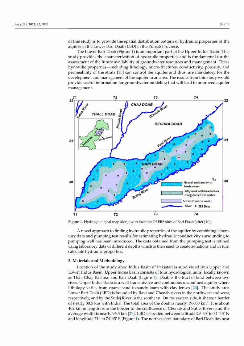
The Lower Bari Doab (Figure 1) is an important part of the Upper Indus Basin. Thisstudy provides the characterization of hydraulic properties and is fundamental for theassessment of the future availability of groundwater resources and management. Thesehydraulic properties—including lithology, micro-fractures, conductivity, porosity, andpermeability of the strata [25] can control the aquifer and thus, are mandatory for thedevelopment and management of the aquifer in an area. The results from this study wouldprovide useful information for groundwater modeling that will lead to improved aquifermanagement.

Figure 1. Hydrogeological map along with location Of ERS sites of Bari Doab (after [10]).

A novel approach to finding hydraulic properties of the aquifer by combining labora-tory data and pumping test results for estimating hydraulic conductivity surrounding topumping well has been introduced. The data obtained from the pumping test is refinedusing laboratory data of different depths which is then used to create zonations and in turncalculate hydraulic properties.

2. Materials and Methodology

Location of the study area: Indus Basin of Pakistan is subdivided into Upper andLower Indus Basin. Upper Indus Basin consists of four hydrological units, locally knownas Thal, Chaj, Rachna, and Bari Doab (Figure 1). Doab is the tract of land between tworives. Upper Indus Basin is a well-transmissive and continuous unconfined aquifer wherelithology varies from coarse sand to sandy loam with clay lenses [26]. The study areaLower Bari Doab (LBD) is bounded by Ravi and Chenab rivers in the northwest and west,respectively, and by the Sutlej River in the southeast. On the eastern side, it shares a borderof nearly 80.5 km with India. The total area of the doab is nearly 19,600 km2. It is about402 km in length from the border to the confluence of Chenab and Sutlej Rivers and theaverage width is nearly 96.5 km [27]. LBD is located between latitude 2930′ to 3145′ Nand longitude 71 to 7445′ E (Figure 1). The northeastern boundary of Bari Doab lies near

Appl. Sci. 2022, 12, 3055 4 of 19

the foothills of the Himalayan range and almost coincides with the Lahore district. LBD isa part of the Indus Basin Irrigation System and comprises a network of canals [28].

Climate: Agriculture is the principal occupation in Lower Bari Doab. There are twoseasons termed Kharif and Rabi. The Kharif season includes the monsoon months startingfrom 15 July to 15 September and the Rabi season is the relatively dry winter season from15 October to 15 April. The climate is arid to semi-arid, and the mean annual precipitationranges from 102 mm in the south to 508 mm in the north. Two-thirds of this precipitationoccurs in the four summer months. Maximum temperature ranges from about 20 C inDecember and January to about 41 C in May and June.

Hydrogeology: Lower Bari Doab is a part of the Indo-Gangetic Plain and is coveredby Quaternary alluvium, which presumably overlies semi-consolidated tertiary rocks ormetamorphic and igneous rocks of Precambrian age [29]. Several deep test holes rangingfrom 243.83 to 396.22 m depth were drilled to determine the thickness of the alluviumand the depth of the bedrock. In these test drills, the bedrock was encountered in onlythree holes at 381.59, 311.19, and 282.84 m in the northeastern part of the Bari Doab [29].Therefore, in the Lower Bari Doab area, the total thickness of the Quaternary alluvium andthe distribution of tertiary and older rocks were not found [30].

The subsurface lithology consists of mainly sand encountered in test holes and waterwells showed the water-bearing characteristic of the alluvial deposits, that form the aquiferof the Bari Doab. A comparative study of the lithological logs provided a fairly good ideaabout the texture and structure of the heterogeneous alluvium to the depth of 183 m. Thesubsurface lithologies inferred in the Quaternary alluvial complex consisted of clay, sandysilt, fine sand, fine-to-medium sand, medium-to-coarse sand, coarse sand, and gravel. Thealluvial material covering the study area formed part of the extensive heterogeneous andisotropic unconfined aquifer underlying the Indus Basin and was believed to be more than304.79 m thick. Geological evidence also indicated that the aquifer is unconfined [31]. Theaquifer yield varies from 100 to 300 m/h in Bari Doab [10] (Figure 1).

Electrical Resistivity Survey: The geoelectrical method measures the distribution ofthe subsurface resistivity which is a physical property depending on the characteristicsof the materials [32]. The principle of the electrical resistivity method is based uponinjection/passage of electric currents into the ground for the discovery of electrical featuresof the materials buried in the ground [33]. This method is quick and cost-effective andhas proven more successful for describing subsurface lithological and hydrogeologicalfeatures [34,35] and groundwater conditions and subsurface layers [36,37]. This method isalso used to estimate the hydrological parameters of the aquifer. Many researchers haveevaluated aquifer parameters using the resistivity method [38–40]. This method has beenutilized for indirect estimation of K and T, reducing the need to drill boreholes that wereused for pumping tests [41–43].

Electrical resistivity survey is a practical application of Ohm’s law, as shown in Equa-tion (1), to map the subsurface changes in earth resistivity and correlate them with thehidden geological formations.

R ∝ ∆V/I · · · or · · · R = K × (∆V/l) (1)

where R is apparent resistivity (ohmmeter); ∆V = Voltage (potential drop) measured inmilli-volt; I = current (milli-ampere); and K = Schlumberger constant of proportionality.

The apparent resistivity depends on the injected current I, measured potential V, andthe geometric factor K [33,44]. Current injected into the subsurface is affected by manyfeatures of the strata such as priority organic components, minerals such as silt, clay, packingof void spaces, fluid presence, etc. in subsurface strata [45]. This method is used profitablyto determine qualitatively the type of water-bearing formation, e.g., sand, sandstone, gravel,boulder provided conditions are favorable and not complicated by abrupt lateral changesin lithology. In resistivity surveys, a commuted direct current is introduced into the groundvia two electrodes (A & B). The potential difference is measured between the second pair ofelectrodes (M & N). The four electrodes are arranged in any of several possible patterns. The

Appl. Sci. 2022, 12, 3055 5 of 19

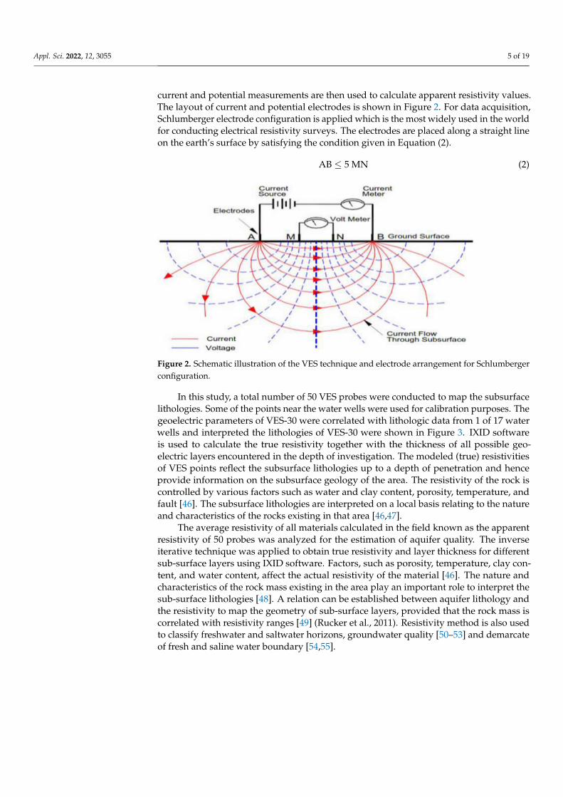
current and potential measurements are then used to calculate apparent resistivity values.The layout of current and potential electrodes is shown in Figure 2. For data acquisition,Schlumberger electrode configuration is applied which is the most widely used in the worldfor conducting electrical resistivity surveys. The electrodes are placed along a straight lineon the earth’s surface by satisfying the condition given in Equation (2).

AB ≤ 5 MN (2)

Figure 2. Schematic illustration of the VES technique and electrode arrangement for Schlumbergerconfiguration.

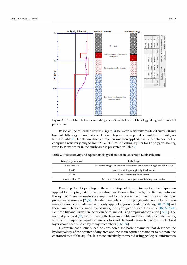
In this study, a total number of 50 VES probes were conducted to map the subsurfacelithologies. Some of the points near the water wells were used for calibration purposes. Thegeoelectric parameters of VES-30 were correlated with lithologic data from 1 of 17 waterwells and interpreted the lithologies of VES-30 were shown in Figure 3. IXID softwareis used to calculate the true resistivity together with the thickness of all possible geo-electric layers encountered in the depth of investigation. The modeled (true) resistivitiesof VES points reflect the subsurface lithologies up to a depth of penetration and henceprovide information on the subsurface geology of the area. The resistivity of the rock iscontrolled by various factors such as water and clay content, porosity, temperature, andfault [46]. The subsurface lithologies are interpreted on a local basis relating to the natureand characteristics of the rocks existing in that area [46,47].

The average resistivity of all materials calculated in the field known as the apparentresistivity of 50 probes was analyzed for the estimation of aquifer quality. The inverseiterative technique was applied to obtain true resistivity and layer thickness for differentsub-surface layers using IXID software. Factors, such as porosity, temperature, clay con-tent, and water content, affect the actual resistivity of the material [46]. The nature andcharacteristics of the rock mass existing in the area play an important role to interpret thesub-surface lithologies [48]. A relation can be established between aquifer lithology andthe resistivity to map the geometry of sub-surface layers, provided that the rock mass iscorrelated with resistivity ranges [49] (Rucker et al., 2011). Resistivity method is also usedto classify freshwater and saltwater horizons, groundwater quality [50–53] and demarcateof fresh and saline water boundary [54,55].

Appl. Sci. 2022, 12, 3055 6 of 19

Figure 3. Correlation between sounding curve-30 with test drill lithology along with modeledparameters.

Based on the calibrated results (Figure 3), between resistivity modeled curve-30 andborehole lithology, a standard correlation of layers was prepared separately for lithologieslisted in Table 2. This standardized correlation was then applied to all VES data points. Thecomputed resistivity ranged from 20 to 90 Ω-m, indicating aquifer for 17 polygons havingfresh to saline water in the study area is presented in Table 2.

Table 2. True resistivity and aquifer lithology calibration in Lower Bari Doab, Pakistan.

Resistivity (ohm-m) Lithology

Less than 20 Silt containing saline water; Dominant sand containing brackish water

20–40 Sand containing marginally fresh water

40–55 Sand containing fresh water

Greater than 55 Mixture of sand and minor gravel containing fresh water

Pumping Test: Depending on the nature/type of the aquifer, various techniques areapplied to pumping data (time drawdown vs. time) to find the hydraulic parameters ofthe aquifer. These parameters are important for the prediction of the future availability ofgroundwater reserves [23,56]. Aquifer parameters including hydraulic conductivity, trans-missivity, and storativity are commonly applied in groundwater modeling [40,57,58] andthese parameters are also estimated using the hydro-geophysical technique [16,56,59,60].Permeability and formation factor can be estimated using empirical correlation [39,61]. Themethod proposed [62] for estimating the transmissibility and storability of aquifers usingspecific well capacity. Aquifer characteristics and electrical parameters of the geoelectricallayers have been studied by many researchers [9,63–66].

Hydraulic conductivity can be considered the basic parameter that describes thehydrogeology of the aquifer of any area and the main aquifer parameter to estimate thecharacteristics of the aquifer. It is more effectively estimated using geological information

Appl. Sci. 2022, 12, 3055 7 of 19

extracted from drilled wells or test hole wells. It governs, along with other parameters, theflow of fluids and the migration of contaminants in the subsurface lithologies. Hydraulicconductivity is a measure of how easily water can pass through soil or rock: high valuesindicate permeable material through which water can pass easily and vice versa.

The Lower Bari Doab (LBD) is part of the Indus Basin is very important for thecharacterization of hydraulic properties, fundamental for the assessment of the futureavailability of groundwater resources and precise management.

To model the behavior of hydraulic conductivity in the aquifer, a grid consisting of66 columns by 26 rows is overlaid on the area with a spacing of 5000 m, both in X- andY-directions. For this purpose, test holes and water wells are used which had been drilledduring different exploration stages by WAPDA. The pumping test data and the hydrauliccharacteristics of these water wells were also studied [31,67,68].

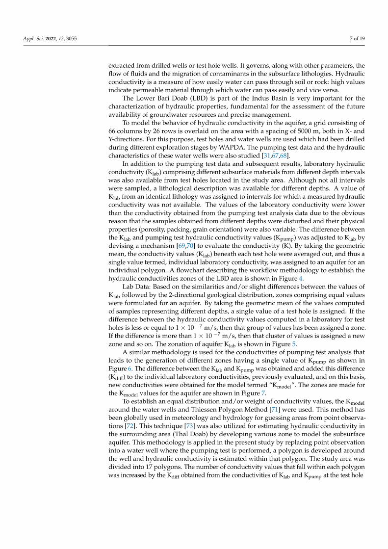
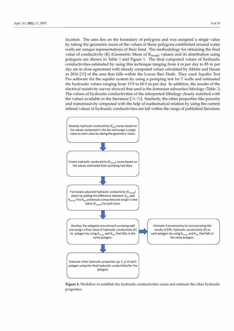
In addition to the pumping test data and subsequent results, laboratory hydraulicconductivity (Klab) comprising different subsurface materials from different depth intervalswas also available from test holes located in the study area. Although not all intervalswere sampled, a lithological description was available for different depths. A value ofKlab from an identical lithology was assigned to intervals for which a measured hydraulicconductivity was not available. The values of the laboratory conductivity were lowerthan the conductivity obtained from the pumping test analysis data due to the obviousreason that the samples obtained from different depths were disturbed and their physicalproperties (porosity, packing, grain orientation) were also variable. The difference betweenthe Klab and pumping test hydraulic conductivity values (Kpump) was adjusted to Klab bydevising a mechanism [69,70] to evaluate the conductivity (K). By taking the geometricmean, the conductivity values (Klab) beneath each test hole were averaged out, and thus asingle value termed, individual laboratory conductivity, was assigned to an aquifer for anindividual polygon. A flowchart describing the workflow methodology to establish thehydraulic conductivities zones of the LBD area is shown in Figure 4.

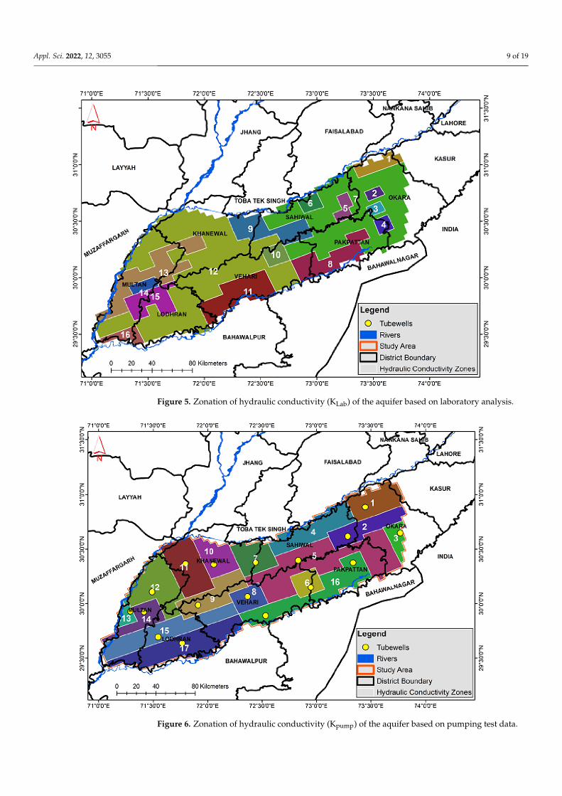
Lab Data: Based on the similarities and/or slight differences between the values ofKlab followed by the 2-directional geological distribution, zones comprising equal valueswere formulated for an aquifer. By taking the geometric mean of the values computedof samples representing different depths, a single value of a test hole is assigned. If thedifference between the hydraulic conductivity values computed in a laboratory for testholes is less or equal to 1 × 10 −7 m/s, then that group of values has been assigned a zone.If the difference is more than 1 × 10 −7 m/s, then that cluster of values is assigned a newzone and so on. The zonation of aquifer Klab is shown in Figure 5.

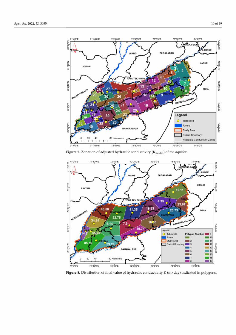
A similar methodology is used for the conductivities of pumping test analysis thatleads to the generation of different zones having a single value of Kpump as shown inFigure 6. The difference between the Klab and Kpump was obtained and added this difference(Kdiff) to the individual laboratory conductivities, previously evaluated, and on this basis,new conductivities were obtained for the model termed “Kmodel”. The zones are made forthe Kmodel values for the aquifer are shown in Figure 7.

To establish an equal distribution and/or weight of conductivity values, the Kmodelaround the water wells and Thiessen Polygon Method [71] were used. This method hasbeen globally used in meteorology and hydrology for guessing areas from point observa-tions [72]. This technique [73] was also utilized for estimating hydraulic conductivity inthe surrounding area (Thal Doab) by developing various zone to model the subsurfaceaquifer. This methodology is applied in the present study by replacing point observationinto a water well where the pumping test is performed, a polygon is developed aroundthe well and hydraulic conductivity is estimated within that polygon. The study area wasdivided into 17 polygons. The number of conductivity values that fall within each polygonwas increased by the Kdiff obtained from the conductivities of Klab and Kpump at the test hole

Appl. Sci. 2022, 12, 3055 8 of 19

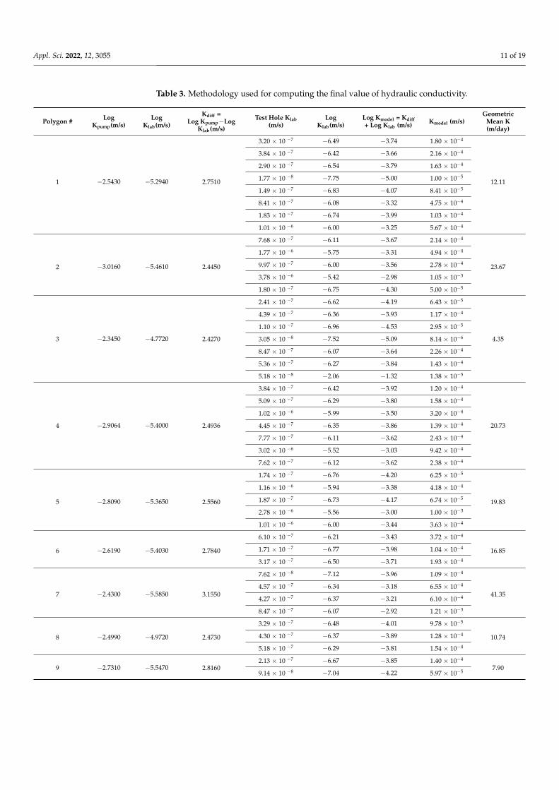
location. The area lies on the boundary of polygons and was assigned a single valueby taking the geometric mean of the values of those polygons established around waterwells are unique representations of their kind. The methodology for obtaining the finalvalue of conductivity (K) (Geometric Mean of Kmodel values) and its distribution usingpolygons are shown in Table 3 and Figure 8. The final computed values of hydraulicconductivities estimated by using this technique ranging from 4 m per day to 85 m perday are in close agreement with already computed values calculated by Akhter and Hasanin 2016 [58] of the area that falls within the Lower Bari Doab. They used Aquifer TestPro software for the aquifer system by using a pumping test for 7 wells and estimatedthe hydraulic values ranging from 15.9 to 60.9 m per day. In addition, the results of theelectrical resistivity survey showed that sand is the dominant subsurface lithology (Table 2).The values of hydraulic conductivities of the interpreted lithology closely matched withthe values available in the literature [74–76]. Similarly, the other properties like porosityand transmissivity computed with the help of mathematical relation by using the currentrefined values of hydraulic conductivities are fall within the range of published literature.

Figure 4. Workflow to establish the hydraulic conductivities zones and estimate the other hydraulicproperties.

Appl. Sci. 2022, 12, 3055 9 of 19

Figure 5. Zonation of hydraulic conductivity (KLab) of the aquifer based on laboratory analysis.

Figure 6. Zonation of hydraulic conductivity (Kpump) of the aquifer based on pumping test data.

Appl. Sci. 2022, 12, 3055 10 of 19

Figure 7. Zonation of adjusted hydraulic conductivity (Kmodel) of the aquifer.

Figure 8. Distribution of final value of hydraulic conductivity K (m/day) indicated in polygons.

Appl. Sci. 2022, 12, 3055 11 of 19

Table 3. Methodology used for computing the final value of hydraulic conductivity.

Polygon # LogKpump(m/s)

LogKlab(m/s)

Kdiff =Log Kpump−Log

Klab(m/s)

Test Hole Klab(m/s)

LogKlab(m/s)

Log Kmodel = Kdiff+ Log Klab (m/s) Kmodel (m/s)

GeometricMean K(m/day)

1 −2.5430 −5.2940 2.7510

3.20 × 10 −7 −6.49 −3.74 1.80 × 10−4

12.11

3.84 × 10 −7 −6.42 −3.66 2.16 × 10−4

2.90 × 10 −7 −6.54 −3.79 1.63 × 10−4

1.77 × 10 −8 −7.75 −5.00 1.00 × 10−5

1.49 × 10 −7 −6.83 −4.07 8.41 × 10−5

8.41 × 10 −7 −6.08 −3.32 4.75 × 10−4

1.83 × 10 −7 −6.74 −3.99 1.03 × 10−4

1.01 × 10 −6 −6.00 −3.25 5.67 × 10−4

2 −3.0160 −5.4610 2.4450

7.68 × 10 −7 −6.11 −3.67 2.14 × 10−4

23.67

1.77 × 10 −6 −5.75 −3.31 4.94 × 10−4

9.97 × 10 −7 −6.00 −3.56 2.78 × 10−4

3.78 × 10 −6 −5.42 −2.98 1.05 × 10−3

1.80 × 10 −7 −6.75 −4.30 5.00 × 10−5

3 −2.3450 −4.7720 2.4270

2.41 × 10 −7 −6.62 −4.19 6.43 × 10−5

4.35

4.39 × 10 −7 −6.36 −3.93 1.17 × 10−4

1.10 × 10 −7 −6.96 −4.53 2.95 × 10−5

3.05 × 10 −8 −7.52 −5.09 8.14 × 10−6

8.47 × 10 −7 −6.07 −3.64 2.26 × 10−4

5.36 × 10 −7 −6.27 −3.84 1.43 × 10−4

5.18 × 10 −8 −2.06 −1.32 1.38 × 10−5

4 −2.9064 −5.4000 2.4936

3.84 × 10 −7 −6.42 −3.92 1.20 × 10−4

20.73

5.09 × 10 −7 −6.29 −3.80 1.58 × 10−4

1.02 × 10 −6 −5.99 −3.50 3.20 × 10−4

4.45 × 10 −7 −6.35 −3.86 1.39 × 10−4

7.77 × 10 −7 −6.11 −3.62 2.43 × 10−4

3.02 × 10 −6 −5.52 −3.03 9.42 × 10−4

7.62 × 10 −7 −6.12 −3.62 2.38 × 10−4

5 −2.8090 −5.3650 2.5560

1.74 × 10 −7 −6.76 −4.20 6.25 × 10−5

19.83

1.16 × 10 −6 −5.94 −3.38 4.18 × 10−4

1.87 × 10 −7 −6.73 −4.17 6.74 × 10−5

2.78 × 10 −6 −5.56 −3.00 1.00 × 10−3

1.01 × 10 −6 −6.00 −3.44 3.63 × 10−4

6 −2.6190 −5.4030 2.7840

6.10 × 10 −7 −6.21 −3.43 3.72 × 10−4

16.851.71 × 10 −7 −6.77 −3.98 1.04 × 10−4

3.17 × 10 −7 −6.50 −3.71 1.93 × 10−4

7 −2.4300 −5.5850 3.1550

7.62 × 10 −8 −7.12 −3.96 1.09 × 10−4

41.354.57 × 10 −7 −6.34 −3.18 6.55 × 10−4

4.27 × 10 −7 −6.37 −3.21 6.10 × 10−4

8.47 × 10 −7 −6.07 −2.92 1.21 × 10−3

8 −2.4990 −4.9720 2.4730

3.29 × 10 −7 −6.48 −4.01 9.78 × 10−5

10.744.30 × 10 −7 −6.37 −3.89 1.28 × 10−4

5.18 × 10 −7 −6.29 −3.81 1.54 × 10−4

9 −2.7310 −5.5470 2.81602.13 × 10 −7 −6.67 −3.85 1.40 × 10−4

7.909.14 × 10 −8 −7.04 −4.22 5.97 × 10−5

Appl. Sci. 2022, 12, 3055 12 of 19

Table 3. Cont.

Polygon # LogKpump(m/s)

LogKlab(m/s)

Kdiff =Log Kpump−Log

Klab(m/s)

Test Hole Klab(m/s)

LogKlab(m/s)

Log Kmodel = Kdiff+ Log Klab (m/s) Kmodel (m/s)

GeometricMean K(m/day)

10 −2.6600 −5.2430 2.5830

2.13 × 10 −7 −6.67 −4.09 8.17 × 10−5

22.75

1.39 × 10 −6 −5.86 −3.27 5.33 × 10−4

4.54 × 10 −7 −6.34 −3.76 1.74 × 10−4

2.14 × 10 −6 −5.67 −3.09 8.17 × 10−4

5.36 × 10 −7 −6.27 −3.69 2.05 × 10−4

11 −2.9010 −5.5050 2.6040

9.14 × 10 −8 −7.04 −4.43 3.66 × 10−5

6.14

3.05 × 10 −8 −7.52 −4.91 1.23 × 10−5

3.81 × 10 −7 −6.42 −3.82 1.53 × 10−4

9.45 × 10 −7 −6.02 −3.42 3.81 × 10−4

1.74 × 10 −7 −6.76 −4.16 6.98 × 10−5

12 −2.9930 −5.6510 2.65802.33 × 10 −6 −5.63 −2.97 1.06 × 10−3

40.564.57 × 10 −7 −6.34 −3.68 2.08 × 10−4

13 −2.7770 −5.4480 2.6710

2.34 × 10 −6 −5.63 −2.96 1.10 × 10−3

34.24

7.01 × 10 −7 −6.15 −3.48 3.29 × 10−4

2.86 × 10 −7 −6.54 −3.87 1.34 × 10−4

5.64 × 10 −6 −5.25 −2.58 2.64 × 10−3

1.65 × 10 −7 −6.78 −4.11 7.71 × 10−5

14 −2.9000 −5.3100 2.41006.10 × 10 −7 −6.21 −3.80 1.57 × 10−4

39.245.15 × 10 −6 −5.29 −2.88 1.32 × 10−3

15 −1.8210 −6.0140 4.19303.05 × 10 −8 −7.52 −3.32 4.75 × 10−4

65.057.62 × 10 −8 −7.12 −2.93 1.19 × 10−3

16 −2.4260 −6.1510 3.7250

3.05 × 10 −8 −7.52 −3.79 1.62 × 10−4

85.593.90 × 10 −6 −5.41 −1.68 2.07 × 10−2

1.34 × 10 −7 −6.87 −3.15 7.13 × 10−4

7.62 × 10 −8 −7.12 −3.39 4.05 × 10−4

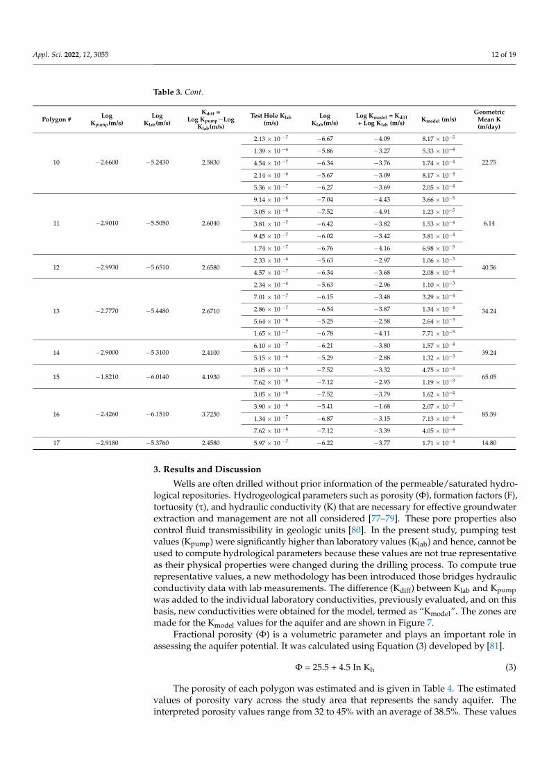
17 −2.9180 −5.3760 2.4580 5.97 × 10 −7 −6.22 −3.77 1.71 × 10−4 14.80

3. Results and Discussion

Wells are often drilled without prior information of the permeable/saturated hydro-logical repositories. Hydrogeological parameters such as porosity (Φ), formation factors (F),tortuosity (τ), and hydraulic conductivity (K) that are necessary for effective groundwaterextraction and management are not all considered [77–79]. These pore properties alsocontrol fluid transmissibility in geologic units [80]. In the present study, pumping testvalues (Kpump) were significantly higher than laboratory values (Klab) and hence, cannot beused to compute hydrological parameters because these values are not true representativeas their physical properties were changed during the drilling process. To compute truerepresentative values, a new methodology has been introduced those bridges hydraulicconductivity data with lab measurements. The difference (Kdiff) between Klab and Kpumpwas added to the individual laboratory conductivities, previously evaluated, and on thisbasis, new conductivities were obtained for the model, termed as “Kmodel”. The zones aremade for the Kmodel values for the aquifer and are shown in Figure 7.

Fractional porosity (Φ) is a volumetric parameter and plays an important role inassessing the aquifer potential. It was calculated using Equation (3) developed by [81].

Φ = 25.5 + 4.5 In Kh (3)

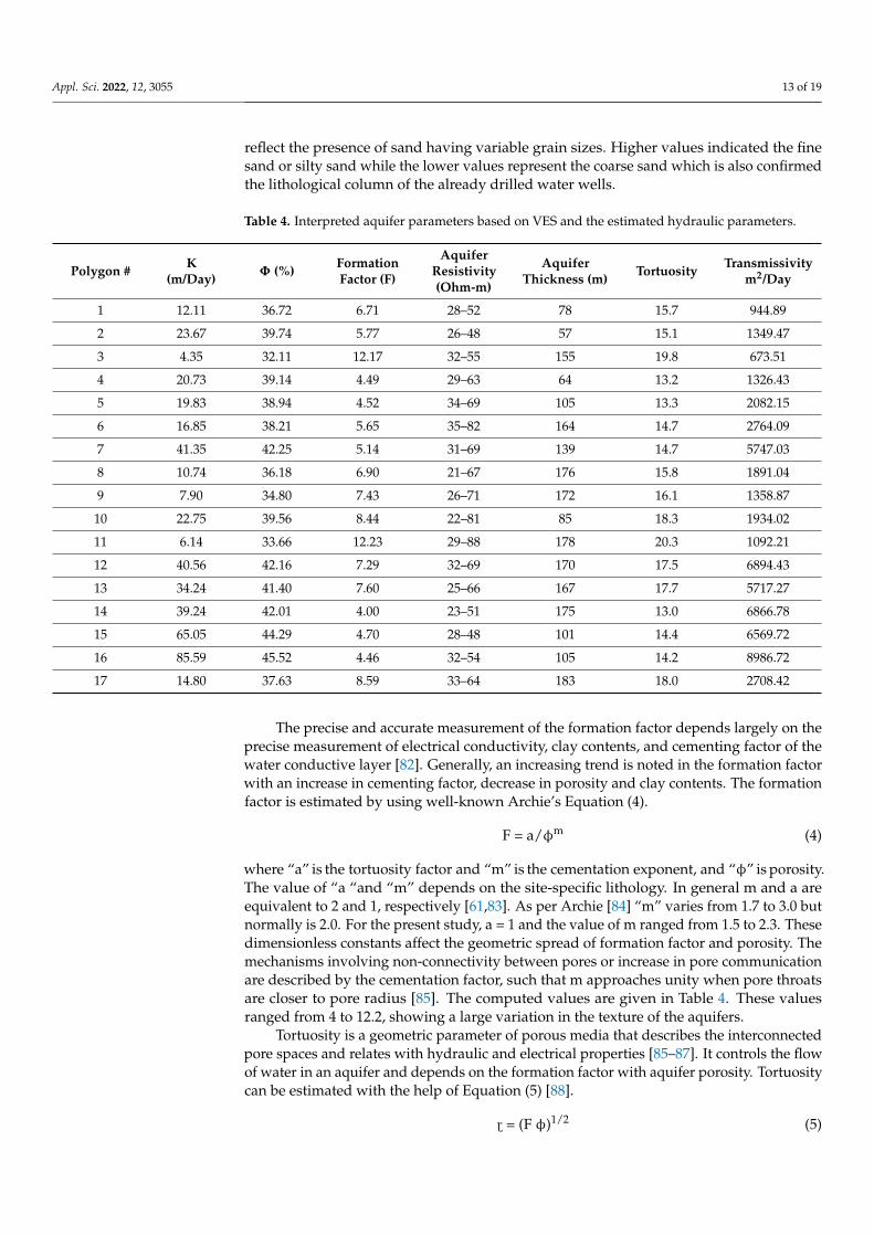
The porosity of each polygon was estimated and is given in Table 4. The estimatedvalues of porosity vary across the study area that represents the sandy aquifer. Theinterpreted porosity values range from 32 to 45% with an average of 38.5%. These values

Appl. Sci. 2022, 12, 3055 13 of 19

reflect the presence of sand having variable grain sizes. Higher values indicated the finesand or silty sand while the lower values represent the coarse sand which is also confirmedthe lithological column of the already drilled water wells.

Table 4. Interpreted aquifer parameters based on VES and the estimated hydraulic parameters.

Polygon # K(m/Day) Φ (%) Formation

Factor (F)

AquiferResistivity(Ohm-m)

AquiferThickness (m) Tortuosity Transmissivity

m2/Day

1 12.11 36.72 6.71 28–52 78 15.7 944.89

2 23.67 39.74 5.77 26–48 57 15.1 1349.47

3 4.35 32.11 12.17 32–55 155 19.8 673.51

4 20.73 39.14 4.49 29–63 64 13.2 1326.43

5 19.83 38.94 4.52 34–69 105 13.3 2082.15

6 16.85 38.21 5.65 35–82 164 14.7 2764.09

7 41.35 42.25 5.14 31–69 139 14.7 5747.03

8 10.74 36.18 6.90 21–67 176 15.8 1891.04

9 7.90 34.80 7.43 26–71 172 16.1 1358.87

10 22.75 39.56 8.44 22–81 85 18.3 1934.02

11 6.14 33.66 12.23 29–88 178 20.3 1092.21

12 40.56 42.16 7.29 32–69 170 17.5 6894.43

13 34.24 41.40 7.60 25–66 167 17.7 5717.27

14 39.24 42.01 4.00 23–51 175 13.0 6866.78

15 65.05 44.29 4.70 28–48 101 14.4 6569.72

16 85.59 45.52 4.46 32–54 105 14.2 8986.72

17 14.80 37.63 8.59 33–64 183 18.0 2708.42

The precise and accurate measurement of the formation factor depends largely on theprecise measurement of electrical conductivity, clay contents, and cementing factor of thewater conductive layer [82]. Generally, an increasing trend is noted in the formation factorwith an increase in cementing factor, decrease in porosity and clay contents. The formationfactor is estimated by using well-known Archie’s Equation (4).

F = a/φm (4)

where “a” is the tortuosity factor and “m” is the cementation exponent, and “φ” is porosity.The value of “a “and “m” depends on the site-specific lithology. In general m and a areequivalent to 2 and 1, respectively [61,83]. As per Archie [84] “m” varies from 1.7 to 3.0 butnormally is 2.0. For the present study, a = 1 and the value of m ranged from 1.5 to 2.3. Thesedimensionless constants affect the geometric spread of formation factor and porosity. Themechanisms involving non-connectivity between pores or increase in pore communicationare described by the cementation factor, such that m approaches unity when pore throatsare closer to pore radius [85]. The computed values are given in Table 4. These valuesranged from 4 to 12.2, showing a large variation in the texture of the aquifers.

Tortuosity is a geometric parameter of porous media that describes the interconnectedpore spaces and relates with hydraulic and electrical properties [85–87]. It controls the flowof water in an aquifer and depends on the formation factor with aquifer porosity. Tortuositycan be estimated with the help of Equation (5) [88].

ó = (F φ)1/2 (5)

Appl. Sci. 2022, 12, 3055 14 of 19

Tortuosity calculated for 17 polygons that represent the area is presented in Table 4.This indicates that high tortuosity corresponds to low porosity and affects aquifer transmis-sibility and pore connectivity. The computed final values of hydraulic conductivity variedfrom 4.5 to 85.6 m/day affect the natural flow of fluids in the aquifer while tortuosity valueranges from 13 to 20.

Transmissivity is an important parameter in assessing the aquifer potential and can becomputed by using Equation (6) [17,64]. It describes the capacity of the aquifer to transmitgroundwater wholly in its entire saturated thickness [89] (Omeje et al., 2021). It can also bedefined as the rate of flow of water through a vertical strip of the aquifer [90].

T = Kb (6)

where K is hydraulic conductivity (m/day) and b is the thickness of the aquifer measuredin meters. The thickness of the aquifer is estimated for each VES by using IXID softwarewhich is given in Table 4. The evaluated thickness of the aquifer varies from 57 to 183 m.The transmissivity values of the aquifer vary in a large range (674 to 8986 m2/day) due tostrong contrast in the aquifer lithology. The very low transmissivity, hydraulic conductivity,and formation factor are associated with fine-grain sediments. These fine-grain sedimentsare mainly sand with silt/minor clay and comprise the aquifer of sandy plain zones.

Apparent resistivity (ρa = ∆V/I* K) computed in the field at different depths is anaverage value of various subsurface layers and does not represent the true electricalcharacteristics of the individual subsurface layer. Since resistivity values exhibit largevariations with some repetition, the number of subsurface layers revealed by the resistivitysurvey do not often match with the results obtained by trial boring. Layers encounteredby trial boring shall be greater in number than layers interpreted by resistivity survey.Apparent resistivity values are not a true representation of the subsurface lithology untilthey are matched with the theoretical master curves drawn manually or through computermodeling. The VES data collected at 50 probes were modeled by using the IXID ComputerSoftware that gives the model interpretation of individual curves stating/reflecting thenumber of layers, their true resistivity values with thickness, and depth from the surface.From 50 points, some of the points are near the existing water well/test holes that wereused for calibration purposes to correlate the true resistivities with subsurface permeableand impervious layers. These standardized values were applied to the rest of the probesand interpreted the subsurface lithologies. Subsurface geological material as depictedfrom resistivity modeling was composed of layers of sand, clay, and silt mixed withgravel/sand. The dominant subsurface encountered at all sites (given in Table 1) consists ofsand containing fresh, saline, and brackish water. The sand formation containing freshwaterindicated high resistivity values as compared to sand containing saline water. The lowerresistivity values less than 20 ohm-m below the water table from comparatively the deeperhorizon indicated the sand containing brackish water whereas the same range of valuesnear the surface indicated the silt containing saline water. After drilling, the aquifer mustbe evaluated in other to determine the aquifer hydraulic properties. These parameters areevaluated with the help of pumping tests that help recommend the capacity of the pumpas well as the depth of installation to improve the life and stabilization of the aquifer. Thepumping test is conducted to examine the aquifer response, under controlled conditions, tothe abstraction of water

The results of the pumping test are considered accurate and are used to evaluate thehydraulic properties. In this study, the hydraulic conductivity of rock samples collected atdifferent depths from test holes was also available, but these values were lower than theconductivity obtained from the pumping test analysis due to the well-known factors thatthe samples obtained from different depths were disturbed and their physical properties(porosity, packing, grain orientation) also changed. To map the hydraulic conductivitylaterally of the investigated area, the values of hydraulic conductivities evaluated from thepumping test with laboratory analysis were utilized by converting the area into 17 polygonswhere the pumping test was conducted. The final values of hydraulic conductivities were

Appl. Sci. 2022, 12, 3055 15 of 19

estimated and are given in Table 3. The estimated hydraulic conductivities that representedthe area falls in the range of 4.4 to 85.6 m/day. The highest value is interpreted at thejunction of the Indus and Sutlej Rivers. This reflects the way they were deposited of thetransported material in nature by rivers. Later, the values of transmissivity have beenestimated by calculating the average thickness of the aquifer with the help of VES data foreach polygon that ranged from 674 to 8986 m2/day. The transmissivity values evaluated foreach polygon are shown in Table 4. Afterward, by using the already established relationshaving the same geological environments, the values of porosity, formation factor, andtortuosity were estimated of the whole investigated area. It is obvious from the results(Table 4) that the hydraulic conductivity increases with the increase in porosity indicatingthe high potential area. The higher values of the porosity are estimated towards thenorthern sides of the area where the Indus and Sutlej Rivers interest each other due to theobvious reason those maximum sediments are deposited at these places.

4. Conclusions

A total of 50 vertical electrical soundings (VES) were analyzed and true resistivitieswith the thickness of individuals have been identified. The results showed that resistivityvalues range from 20 to90 ohm-m with a minimum thickness of 57 m while the maximumthickness of 178 m of unconfined aquifer material consists of dominant sand containingfresh, marginally fresh, and brackish water. Further based on true resistivity values variousaquifer regions of fresh, brackish, and saline water were differentiated. The lithologyconsists of silt/clay having resistivity <20 ohm-m representing saline water. Sand con-taining marginally fresh water and freshwater having resistivity 20–40 and 40–55 ohm-m,respectively. Whereas a mixture of sand and gravel containing freshwater having resistivityvalues ranged from 55–90 ohmmeters. Based on this standardization (Table 2), the waterquality at different depths has been interpreted based on true resistivity values. Thiscalibration shows the intermixing of resistivity values for subsurface layers, which causeoverlapping of fresh–brackish and brackish–saline groundwater zones.

Hydraulic properties of the area were estimated by using the pumping test data, hy-draulic conductivities estimated in the lab, VES data, and previously established regressionequation. In the current study, the focus was to evaluate the hydraulic conductivity andafterward transmissivity, porosity, formation factor, and tortuosity based on the estimatedvalue of K. The estimated hydraulic conductivity, transmissivity, porosity, formation factor,and tortuosity values of the aquifer range from 4.4 to 85.6 m/day, 674 to 8986 m2/day,32 to 45 %, 4 to 12, and 13 to 20, respectively. Higher hydraulic conductivities were encoun-tered in the southern portion of the area near the junction of the river as compared to therest of the area. The porosity is also in an increasing trend. It is also concluded that thepolygons representing aquifer having T > 5700 m2/day and K > 40 m/day, are consideredexcellent aquifer which can yield a large quantity of water. On the other hand, the polygonswith T < 1100 m2/day and K < 13 m/day are considered combatively low yield aquifer.

Author Contributions: Conceptualization, G.A. and Y.G.; methodology, G.A.; software, G.A., M.H.;validation, G.A., Y.S. and Y.G.; formal analysis, M.H., G.A.; investigation, G.A. and Y.G.; resources, Y.G.and Y.S.; data curation, Y.S. and M.H.; writing—original draft preparation, M.H. and Y.G.; writing—review and editing, G.A. and Y.S.; visualization, G.A.; supervision, Y.G.; project administration, Y.G.;funding acquisition, Y.G. All authors have read and agreed to the published version of the manuscript.

Funding: This research is financially supported by the Chinese Academy of Sciences President’s Inter-national Fellowship Initiative (Grant No. 2021VCA0010) and the International Science & TechnologyCooperation Program of China (2018YFE0100100).

Institutional Review Board Statement: Not applicable.

Informed Consent Statement: Not applicable.

Data Availability Statement: Not applicable.

Appl. Sci. 2022, 12, 3055 16 of 19

Acknowledgments: The authors wish to acknowledge the Chinese Academy of Sciences President’sInternational Fellowship Initiative and the International Science & Technology Cooperation Programof China financially supported the current research. The authors would like to greatly acknowledgethe support extended by the Director (Hydrology) Of PCRWR. Special thanks of gratitude to theDirector and Executive Director of China-Pakistan Joint Research Centre (CPJRC) on Earth Sciencesfor their encouragement, support during the entire period of research.

Conflicts of Interest: No conflict of interest.

References1. Alam, U.; Sahota, P.; Jeffrey, P. Irrigation in the Indus basin: A history of unsustainability? Water Supply 2007, 7, 211–218.

[CrossRef]2. Watto, M.A. The Economics of Groundwater Irrigation in the Indus Basin, Pakistan: Tube-Well Adoption, Technical and Irrigation

Water Efficiency and Optimal Allocation. Ph.D. Thesis, University of Western Australia, Perth, Australia, 2015.3. Mondal, P.; Dalai, A.K. Sustainable Utilization of Natural Resources; CRC Press: Boca Raton, FL, USA, 2017. [CrossRef]4. Yu, W.H.; Yang, Y.-C.; Savitsky, A.; Alford, D.; Brown, C. The Indus Basin of Pakistan: The Impacts of Climate Risks on Water and

Agriculture; World Bank Publications: Herndon, VA, USA, 2013; Available online: http://hdl.handle.net/10986/13834 (accessedon 10 January 2022).

5. Mukherjee, A. Overview of the groundwater of South Asia. In Groundwater of South Asia; Springer Science and Business Media LLC:Dordrecht, The Netherlands, 2018; pp. 3–20. Available online: https://link.springer.com/chapter/10.1007/978-981-10-3889-1_1(accessed on 10 January 2022).

6. Bakhsh, A.; Awan, Q. Water issues in Pakistan and their remedies. In Proceedings of the National Symposium on Drought andWater Resources in Pakistan, Punjab, Pakistan, 16 March 2002; pp. 145–150.

7. Bakhsh, A.; Kanwar, R.S.; Pederson, C.; Bailey, T.B. N-Source Effects on Temporal Distribution of NO3-N Leaching Losses toSubsurface Drainage Water. Water Air Soil Pollut. 2007, 181, 35–50. [CrossRef]

8. Saeed, M. Skimming Wells; Higher Education Commission: Islamabad, Pakistan, 2008.9. Sikandar, P.; Christen, E.W. Geoelectrical Sounding for the Estimation of Hydraulic Conductivity of Alluvial Aquifers. Water

Resour. Manag. 2012, 26, 1201–1215. [CrossRef]10. Hasan, M.; Shang, Y.; Akhter, G.; Jin, W. Application of VES and ERT for delineation of fresh-saline interface in alluvial aquifers

of Lower Bari Doab, Pakistan. J. Appl. Geophys. 2019, 164, 200–213. [CrossRef]11. Greenman, D.; Swarzenski, W.; Bennett, G. Ground-Water Hydrology of the Punjab Region of West Pakistan, with Emphasis on Problems

Caused by Canal Irrigation; WASID Bulletin 6; West Pakistan Water and Power Development Authority: Punjab, Pakistan, 1967.Available online: https://pubs.er.usgs.gov/publication/wsp1608H (accessed on 10 January 2022).

12. Ahmad, N. Waterlogging and Salinity Problems in Pakistan; Government of Pakistan, Scientific and Technological Research Division,Irrigation, Drainage and Flood Control Research Council: Islamabad, Pakistan, 1974. Available online: https://books.google.com.sg/books/about/Waterlogging_and_Salinity_Problems_in_Pa.html?id=HD5EAAAAYAAJ&redir_esc=y (accessed on 10 January 2022).

13. Alam, K. A groundwater flow model of the Lahore City and its surroundings. In Proceedings of the Regional Workshop onArtificial Groundwater Recharge, Quetta, Pakistan, 10–14 June 1996; pp. 10–14.

14. Mashadi, S.; Mohammad, A. Recharge the depleting aquifer of Lahore Metropolis. In Proceedings of the Regional GroundwaterManagement Seminar, Islamabad, Pakistan, 9–11 October 2000; pp. 209–220.

15. Qureshi, A.S.; Gill, M.A.; Sarwar, A. Sustainable groundwater management in Pakistan: Challenges and opportunities.Irrig. Drain. J. Int. Comm. Irrig. Drain. 2010, 59, 107–116. [CrossRef]

16. Soupios, P.M.; Kouli, M.; Vallianatos, F.; Vafidis, A.; Stavroulakis, G. Estimation of aquifer hydraulic parameters from surficialgeophysical methods: A case study of Keritis Basin in Chania (Crete—Greece). J. Hydrol. 2007, 338, 122–131. [CrossRef]

17. Fetter, C. Applied Hydrogeology, 3rd ed.; University of Wisconsin-Oshkosh, Mc Millian College Publishing Company: New York,NY, USA, 1994.

18. Bowling, J.C.; Rodriguez, A.B.; Harry, D.L.; Zheng, C. Delineating Alluvial Aquifer Heterogeneity Using Resistivity and GPRData. Ground Water 2005, 43, 890–903. [CrossRef] [PubMed]

19. Chowdhury, A.; Jha, M.K.; Chowdary, V.M. Delineation of groundwater recharge zones and identification of artificial rechargesites in West Medinipur district, West Bengal, using RS, GIS and MCDM techniques. Environ. Earth Sci. 2010, 59, 1209–1222.[CrossRef]

20. Lee, S.; Kim, Y.-S.; Oh, H.-J. Application of a weights-of-evidence method and GIS to regional groundwater productivity potentialmapping. J. Environ. Manag. 2012, 96, 91–105. [CrossRef] [PubMed]

21. Nwachukwu, M.A.; Feng, H.; Achilike, K. Integrated study for automobile wastes management and environmentally friendlymechanic villages in the Imo River Basin, Nigeria. Afr. J. Environ. Sci. Technol. 2010, 4, 4.

22. Naghibi, S.A.; Pourghasemi, H.R.; Dixon, B. GIS-based groundwater potential mapping using boosted regression tree, classifica-tion and regression tree, and random forest machine learning models in Iran. Environ. Monit. Assess. 2016, 188, 44. [CrossRef][PubMed]

Appl. Sci. 2022, 12, 3055 17 of 19

23. Hasan, M.; Shang, Y.; Jin, W.; Akhter, G. Geophysical investigation of a weathered terrain for groundwater exploitation: A casestudy from Huidong County, China. Explor. Geophys. 2021, 52, 273–293. [CrossRef]

24. Akhtar, N.; Mislan, M.S.; I Syakir, M.; Anees, M.T.; Yusuff, M.S.M. Characterization of aquifer system using electrical resistivitytomography (ERT) and induced polarization (IP) techniques. IOP Conf. Ser. Earth Environ. Sci. 2021, 880, 012025. [CrossRef]

25. Bowling, J.C.; Harry, D.L.; Rodriguez, A.B.; Zheng, C. Integrated geophysical and geological investigation of a heterogeneousfluvial aquifer in Columbus Mississippi. J. Appl. Geophys. 2007, 62, 58–73. [CrossRef]

26. Iqbal, N.; Hossain, F.; Lee, H.; Akhter, G. Integrated groundwater resource management in Indus Basin using satellite gravimetryand physical modeling tools. Environ. Monit. Assess. 2017, 189, 128. [CrossRef] [PubMed]

27. Bhatti, S.A. Analysis of Aquifer Characteristics and Probable Lowering of Water Levels in Bari Doab; Wasid Publication No. 63; WAPDA:Lahore, Pakistan, 1969.

28. Akhter, G.; Ge, Y.; Iqbal, N.; Shang, Y.; Hasan, M. Appraisal of Remote Sensing Technology for Groundwater ResourceManagement Perspective in Indus Basin. Sustainability 2021, 13, 9686. [CrossRef]

29. Water and Power Development Authority (WAPDA). Hydrogeological Data of Bari Doab (No. Vol.1, Pub. No. 27); DirectorateGeneral of Hydrogeology WAPDA: Lahore, Pakistan, 1980.

30. Kidwai, Z.D.; Alam, S. The Geology of Bari Doab, West Pakistan (Bulletin#8); Water and Power Development Authority (WAPDA):Punjab, Pakistan, 1964.

31. Bennett, G.D.; Rehman, A.-U.; Sheikh, I.A.; Alr, S. Analysis of Aquifer Tests in the Punjab Region of West Pakistan. US GeologicalSurvey: 1967. Available online: https://pubs.er.usgs.gov/publication/wsp1608G (accessed on 10 January 2022).

32. Store, H.; Storz, W.; Jacobs, F. Electrical resistivity tomography to investigate geological structures of the earth’s upper crust.Geophys. Prospect. 2000, 48, 455–471. [CrossRef]

33. Kearey, P.; Brooks, M.; Hill, I. An Introduction to Geophysical Exploration; John Wiley & Sons: Hoboken, NJ, USA, 2002. ISBN 978-0-632-04929-5. Available online: https://faculty.ksu.edu.sa/sites/default/files/AN_INTRODUCTION_TO_GEOPHYSICAL_EXPLORATION_brooks_0_0.pdf (accessed on 10 January 2022).

34. Mondal, N.C.; Singh, V.P.; Ahmed, S. Delineating shallow saline groundwater zones from Southern India using geophysicalindicators. Environ. Monit. Assess. 2012, 185, 4869–4886. [CrossRef]

35. Grygar, T.M.; Elznicová, J.; Tumová, Š.; Famera, M.; Balogh, M.; Kiss, T. Floodplain architecture of an actively meanderingriver (the Ploucnice River, the Czech Republic) as revealed by the distribution of pollution and electrical resistivity tomography.Geomorphology 2016, 254, 41–56. [CrossRef]

36. Lashkaripour, G.R.; Ghafoori, M.; Dehghani, A. Electrical resistivity survey for predicting Samsor aquifer properties, SoutheastIran. In Proceedings of the Geophysical Research Abstracts European Geosciences Union, Vienna, Austria, 24–29 April 2005.Available online: https://www.semanticscholar.org/paper/Electrical-resistivity-survey-for-predicting-Samsor-Lashkaripour-Ghafoori/54824cd84005ab12c3b7d10510ac697f2489626d (accessed on 10 January 2022).

37. Oseji, J.; Asokhia, M.; Okolie, E. Determination of groundwater potential in obiaruku and environs using surface geoelectricsounding. Environmentalist 2006, 26, 301–308. [CrossRef]

38. Bussian, A.E. Electrical conductance in a porous medium. Geophysics 1983, 48, 1258–1268. [CrossRef]39. Senthil, K.M.; Gnanasundar, D.; Elango, L. Geophysical studies in determining hydraulic characteristics of an alluvial aquifer.

J. Environ. Hydrol. 2001, 9, 1–8.40. Singh, K. Nonlinear estimation of aquifer parameters from surficial resistivity measurements. Hydrol. Earth Syst. Sci. Discuss.

2005, 2, 917–938.41. Moreira, C.A.; Cavalheiro, M.L.D.; Pereira, A.M.; Caron, F. Relações entre condutividade hidráulica, transmissividade, con-

dutância longitudinal e sólidos totais dissolvidos para o aquífero livre de Caçapava do Sul (RS), Brasil. Eng. Sanit. Ambient. 2012,17, 193–202. [CrossRef]

42. Choo, H.; Kim, J.; Lee, W.; Lee, C. Relationship between hydraulic conductivity and formation factor of coarse-grained soils as afunction of particle size. J. Appl. Geophys. 2016, 127, 91–101. [CrossRef]

43. Rosa, F.T.; Moreira, C.A.; Carrara, A.; dos Santos, S.F. Análise das relações entre resistividade elétrica, condutividade hidráulica eparâmetros físico-químicos para o Aquífero Livre da Região de Corumbataí (SP). Águas Subterrâneas 2017, 31, 384–392. [CrossRef]

44. Hasan, M.; Shang, Y.; Akhter, G.; Khan, M. Geophysical Investigation of Fresh-Saline Water Interface: A Case Study from SouthPunjab, Pakistan. Ground Water 2017, 55, 841–856. [CrossRef] [PubMed]

45. Dhakate, R.; Chowdhary, D.K.; Rao, V.V.S.G.; Tiwary, R.K.; Sinha, A. Geophysical and geomorphological approach for locatinggroundwater potential zones in Sukinda chromite mining area. Environ. Earth Sci. 2012, 66, 2311–2325. [CrossRef]

46. Gao, Q.; Shang, Y.; Hasan, M.; Jin, W.; Yang, P. Evaluation of a Weathered Rock Aquifer Using ERT Method in South Guangdong,China. Water 2018, 10, 293. [CrossRef]

47. Loke, M.; Barker, R. Rapid least-squares inversion of apparent resistivity pseudosections by a quasi-Newton method1. Geophys.Prospect. 1996, 44, 131–152. [CrossRef]

48. Robinson, E.S. Basic Exploration Geophysics; John Wiley & Sons: New York, NY, USA, 1988.49. Rucker, D.; Noonan, G.E.; Greenwood, W.J. Electrical resistivity in support of geological mapping along the Panama Canal. Eng. Geol.

2011, 117, 121–133. [CrossRef]50. Balasubramanian, A.; Sharma, K.; SASTRI, J.V. Geoelectrical and hydrogeochemical evaluation of coastal aquifers of Tambraparni

basin, Tamil Nadu. Geophys. Res. Bull. 1985, 23, 203–209.

Appl. Sci. 2022, 12, 3055 18 of 19

51. Devaraj, N.; Chidambaram, S.; Panda, B.; Thivya, C.; Thilagavathi, R.; Ganesh, N. Geo-electrical approach to determine the lithologicalcontact and groundwater quality along the KT boundary of Tamilnadu, India. Model. Earth Syst. Environ. 2018, 4, 269–279. [CrossRef]

52. Hussain, Y.; Ullah, S.F.; Akhter, G.; Aslam, A.Q. Groundwater quality evaluation by electrical resistivity method for optimizedtubewell site selection in an ago-stressed Thal Doab Aquifer in Pakistan. Model. Earth Syst. Environ. 2017, 3, 15. [CrossRef]

53. Sonkamble, S. Electrical resistivity and hydrochemical indicators distinguishing chemical characteristics of subsurface pollutionat Cuddalore coast, Tamil Nadu. J. Geol. Soc. India 2014, 83, 535–548. [CrossRef]

54. Adepelumi, A.A.; Ako, B.D.; Ajayi, T.R.; Afolabi, O.; Omotoso, E.J. Delineation of saltwater intrusion into the freshwater aquiferof Lekki Peninsula, Lagos, Nigeria. Environ. Earth Sci. 2009, 56, 927–933. [CrossRef]

55. Batayneh, A.T. Use of electrical resistivity methods for detecting subsurface fresh and saline water and delineating their interfacialconfiguration: A case study of the eastern Dead Sea coastal aquifers, Jordan. Appl. Hydrogeol. 2006, 14, 1277–1283. [CrossRef]

56. Suprapti, A.; Pongmanda, S. Estimation of aquifer parameters using pumping tests: Case study of hotel Makassar paradise.IOP Conf. Ser. Earth Environ. Sci. 2020, 419, 012118. [CrossRef]

57. Freeze, R.A.; Cherry, J.A. Groundwater; Prentice-Hall, Inc.: Englewood Cliffs, NJ, USA, 1979.58. Akhter, G.; Hasan, M. Determination of aquifer parameters using geoelectrical sounding and pumping test data in Khanewal

District, Pakistan. Open Geosci. 2016, 8, 630–638. [CrossRef]59. Lesmes, D.P.; Friedman, S.P. Relationships between the Electrical and Hydrogeological Properties of Rocks and Soils; Springer Science

and Business Media LLC: Dordrecht, The Netherlands, 2005; pp. 87–128.60. Kouamé, I.K.; Douagui, A.G.; Bouatrin, D.K.; Kouadio, S.K.A.; Savané, I. Assessing the hydrodynamic properties of the fissured

layer of granitoid aquifers in the Tchologo Region (Northern Côte d’Ivoire). Heliyon 2021, 7, 07620. [CrossRef] [PubMed]61. Heigold, P.C.; Gilkeson, R.H.; Cartwright, K.; Reed, P.C. Aquifer Transmissivity from Surficial Electrical Methods. Ground Water

1979, 17, 338–345. [CrossRef]62. Chenini, I.; Rafini, S.; Ben Mammou, A. A Simple Method to Estimate Transmissibility and Storativity of Aquifer Using Specific

Capacity of Wells. J. Appl. Sci. 2008, 8, 2640–2643. [CrossRef]63. Olatunji, S.; Musa, A. Estimation of Aquifer Hydraulic Characteristics from Surface Geoelectrical Methods: Case Study of the

Rima Basin, Northwestern Nigeria. Arab. J. Sci. Eng. 2014, 39, 5475–5487. [CrossRef]64. Okiongbo, K.S.; Mebine, P. Estimation of aquifer hydraulic parameters from geoelectrical method—A case study of Yenagoa and

environs, Southern Nigeria. Arab. J. Geosci. 2014, 8, 6085–6093. [CrossRef]65. Khalilidermani, M.; Knez, D.; Zamani, M.A.M. Empirical Correlations between the Hydraulic Properties Obtained from the

Geoelectrical Methods and Water Well Data of Arak Aquifer. Energies 2021, 14, 5415. [CrossRef]66. Türkkan, G.E.; Korkmaz, S. Relationship between hydraulic and geoelectrical parameters for alluvial aquifers in Bursa, Turkey—A

case study. Arab. J. Geosci. 2021, 14, 2221. [CrossRef]67. Water and Power Development Authority (WAPDA). Hydrogeological Data of Bari Doab (Vol-II, Directorate General of Hydrogeology

WAPDA); WAPDA: Lahore, Pakistan, 1982.68. Shahid, M.D. Hydraulic Conductivity contouring by the analysis of aquifer tests and lithologic logs in Bari Doab area. Bull. Pak.

Counc. Res. Water Resour. 1990, 20, 1.69. Ahmad, Z. Numerical Ground water modelling of Rechna Doab flow system. In Proceedings of the Conference PCRWR,

Islamabad, Pakistan, 6–9 December 2000.70. Ahmad, Z. Prickett and Lonnquist Finite Difference Basic Aquifer Simulation Program for Wet and Dry Season, 2nd Golden Software,

Version 5; Department of Geological Sciences, University of Kentucky: Lexington, KY, USA, 1992.71. Theissen, A.H. Precipitation average for large areas. Mon. Wea. Rev. 1911, 39, 1082–1084. [CrossRef]72. Rhynsburger, D. Analytic Delineation of Thiessen Polygons. Geogr. Anal. 1973, 5, 133–144. [CrossRef]73. Mujtaba, G. Conjunctive Use of Geographic Information System (GIS) and 3-D Numerical Models (FEEFLOW) to Characterize

the Groundwater Flow Regimes of the Lower Thal Doab, Punjab, Pakistan. Ph.D. Thesis, Quaid-i-Azam University, Islamabad,Pakistan, 2013.

74. Hölting, B.; Coldewey, W.G. Hydrogeology; Spriger: Berlin/Heidelberg, Germany, 2019; 24p.75. Domenico, P.A.; Schwartz, F.W. Physical and Chemical Hydrogeology; John Wiley & Sons: New York, NY, USA, 1990.76. Todd, D.K. Groundwater Hydrology, 3rd ed.; John Wiley & Sons: Hoboken, NJ, USA, 2015; p. 93. ISBN 978-0-471-05937-0. Available

online: https://www.wiley.com/en-ie/Groundwater+Hydrology,+3rd+Edition-p-9780471059370 (accessed on 10 January 2022).77. Martínez, A.G.; Takahashi, K.; Núñez, E.; Silva, Y.; Trasmonte, G.; Mosquera, K.; Lagos, P. A multi-institutional and interdisci-

plinary approach to the assessment of vulnerability and adaptation to climate change in the Peruvian Central Andes: Problemsand prospects. Adv. Geosci. 2008, 14, 257–260. [CrossRef]

78. Ebong, E.; Akpan, A.E.; Onwuegbuche, A.A. Estimation of geohydraulic parameters from fractured shales and sandstone aquifersof Abi (Nigeria) using electrical resistivity and hydrogeologic measurements. J. Afr. Earth Sci. 2014, 96, 99–109. [CrossRef]

79. Akpan, A.E.; Ugbaja, A.N.; George, N.J. Integrated geophysical, geochemical, and hydrogeological investigation of shallowgroundwater resources in parts of the Ikom-Mamfe Embayment and the adjoining areas in Cross River State, Nigeria. Environ.Earth Sci. 2013, 70, 1435–1456. [CrossRef]

80. George, N.J.; Ibuot, J.C.; Obiora, D.N. Geoelectrohydraulic parameters of shallow sandy aquifer in Itu, Akwa Ibom State (Nigeria)using geoelectric and hydrogeological measurements. J. Afr. Earth Sci. 2015, 110, 52–63. [CrossRef]

Appl. Sci. 2022, 12, 3055 19 of 19

81. Marotz, G. Techische Grundlageneiner Wasserspeicherung Imm Naturlichen Untergrund Habilitationsschrift. Ph.D. Thesis,Universitat Stuttgart, Stuttgart, Germany, 1968.

82. Khalili, M.; Brissette, F.; Leconte, R. Stochastic multi-site generation of daily weather data. Stoch. Hydrol. Hydraul. 2009, 23, 837–849.[CrossRef]

83. Worthington, P.F. The uses and abuses of the Archie equations, 1: The formation factor-porosity relationship. J. Appl. Geophys.1993, 30, 215–228. [CrossRef]

84. Archie, G.E. Classification of carbonate reservoir rocks and petrophysical considerations. Aapg Bull. 1952, 36, 278–298.85. Aleke, C.G.; Ibuot, J.C.; Obiora, D.N. Application of electrical resistivity method in estimating geohydraulic properties of a sandy

hydrolithofacies: A case study of Ajali Sandstone in Ninth Mile, Enugu State, Nigeria. Arab. J. Geosci. 2018, 11, 322. [CrossRef]86. Clennell, M.B. Tortuosity: A guide through the maze. Geol. Soc. Lond. Spec. Publ. 1997, 122, 299–344. [CrossRef]87. Matyka, M.; Khalili, A.; Koza, Z. Tortuosity-porosity relation in porous media flow. Phys. Rev. E 2008, 78, 026306. [CrossRef]

[PubMed]88. The Netherland Organization. Geophysical Well Logging for Geohydrological Purposes in Unconsolidated Formations; Groundwater

Survey TNO; The Netherlands Organisation for Applied Scientific Research: Delft, The Netherlands, 1976.89. Omeje, E.T.; Ugbor, D.O.; Ibuot, J.C.; Obiora, D.N. Assessment of groundwater repositories in Edem, Southeastern Nigeria, using

vertical electrical sounding. Arab. J. Geosci. 2021, 14, 421. [CrossRef]90. George, N.J.; Ibuot, J.C.; Ekanem, A.M.; George, A.M. Estimating the indices of inter-transmissibility magnitude of active surficial

hydrogeologic units in Itu, Akwa Ibom State, southern Nigeria. Arab. J. Geosci. 2018, 11, 134. [CrossRef]