Estimation of Causal Eects in Experiments with Multiple Sources of Noncompliance

Estimation of Causal Effects in Experiments with

Multiple Sources of Noncompliance∗

John Engberg, Dennis Epple, Jason Imbrogno, Holger Sieg

and Ron Zimmer

February 23, 2009

∗John Engberg is a research scientist at the RAND Corporation, Pittsburgh, PA 15213.

Dennis Epple is the Thomas Lord Professor of Economics, Holger Sieg is Professor of Eco-

nomics, Jason Imbrogno is a Ph.D. student at Carnegie Mellon University, Tepper School of

Business, Pittsburgh, PA 15213. Ron Zimmer is an Associate Professor at Michigan State

University, College of Education, East Lansing, MI 48824. We would like to thank Mark

Roosevelt, Superintendent of the Pittsburgh Public Schools, for supporting this research

and granting us access the PPS database. We would also like to thank Stefan Holderlein,

Guido Imbens, Blaise Melly, Robert Moffitt, Chris Taber, Ken Wolpin, Tiemen Woutersen,

and seminar participants at UT Austin, Brown University, Carnegie Mellon University,

Johns Hopkins University, the University of Wisconsin-Madison, and the 5th Conference of

German Economists Abroad in Bonn for comments. Financial support for this research is

provided by the Institute of Education Sciences (IES R305A070117).

Abstract

The purpose of this paper is to study identification and estimation of causal ef-

fects in experiments with multiple sources of noncompliance. This research design

arises in many applications in education when access to oversubscribed programs is

partially determined by randomization. Eligible households decide whether or not

to comply with the intended treatment. The paper treats program participation as

the outcome of a decision process with five latent household types. We show that

the parameters of the underlying model of program participation are identified. Our

proofs of identification are constructive and can be used to design a GMM estimator

for all parameters of interest. We apply our new methods to study the effectiveness

of magnet programs in a large urban school district. Our findings show that magnet

programs help the district to attract and retain students from households that are at

risk of leaving the district. These households have higher incomes, are more educated,

and have children that score higher on standardized tests than households that stay

in district regardless of the outcome of the lottery.

Keywords: Causal Effects, Treatment Effects, Noncompliance, Program Evaluation,

Randomized Experiments, Instrumental Variables, Magnet Programs, Urban School

District, School Choice.

JEL classification: C21, I21, H75

1 Introduction

The purpose of this paper is to study identification and estimation of causal effects

in experiments with multiple sources of noncompliance. In a standard experimental

design, each subject agrees to participate in the experiment and randomization com-

pletely determines whether the individual is assigned to the treatment or the control

group.1 In our design, randomization gives potential participants the option to par-

ticipate in the program, i.e. individuals that win a lottery can choose whether or not

to participate in the program. Individuals thus decide whether or not to comply with

the intended treatment. This type of research design arises in many applications in

education.2 Many school districts use lotteries to determine access to over-subscribed

educational programs. Lottery winners are accepted into the program, with the ulti-

mate choice of attendance left to the student and his family. Households have many

different outside options and as consequence there are different reasons for noncom-

pliance. Lottery losers do not have the option to participate in the program. Program

participation then depends on lottery outcomes as well as on household decisions.

We follow the literature on program evaluation and allow for heterogeneity in the

effect of treatment. This approach was introduced into economics by Quandt (1972),

Heckman (1978) and Lee (1979).3 This approach shares many similarities with the

causal model of potential outcomes introduced by Rubin (1974) into the statistical

literature. Our approach of modeling noncompliance in experimental designs builds

on the work by Angrist, Imbens, and Rubin (1996) (AIR) who also study an ex-

1See, for example, Heckman and Vytlacil (2007) for an overview of the program evaluation

literature.2Angrist (1990) introduced the use of lotteries to study the impact of military service on earnings.

Of course, in his application program participation is mandatory: the penalties of avoiding the draft

were quite significant.3Heckman and Robb (1985) and Bjorklund and Moffitt (1987) treated heterogeneity in treatment

as a random coefficients model.

1

perimental design in which compliance is not perfect: some individuals assigned to

treatment do not take it, and some not assigned to treatment do take it. They refer

to the two non-complying types as “never-takers” and “always-takers.” There is also

a third type that does exactly what its assignment requires. These are referred to as

“compliers.”

Our approach focuses on experimental designs that arise in educational economics.

Our application focuses on the effectiveness of magnet programs. To study these

experimental designs, we generalizes the framework by allowing for additional types

of non-compliance. These additional types arise because households face two outside

options: they can send their children to a non-magnet school within the school district

or they can leave the school district. If there are no schooling options outside the the

public school district, our model simplifies to the one considered in AIR.

Since we need to account for two different sources of non-compliance, our model

has five latent types. The first type is a “complying stayer” who chooses the magnet

program if it wins. The second type is a “non-complying stayer” who does not choose

the magnet program even if he wins the lottery. Both of these types stay in the

district whether they lose the lottery.4 The third and forth types leave the district

if they lose the lottery. The third type is a “leaver” and will not enroll its child in

the district independently of the outcome of the lottery.5 The fourth type complies

with the lottery and participates in the magnet program if it wins the lottery. We

denote these households as “at risk.” Given that many urban school districts are

4The district offers a standard education program to all households that do not win the lottery.5Households have incomplete information and need to gather information to learn about the

features of different programs. Households have to sign up for lotteries months in advance. At that

point, they dot not have accumulated all relevant information. Once they have accumulated all

relevant information, they may decide to opt out of the public school system since their preferred

choice dominates the program offer by the district. Note that there are typically no penalties in

participating in the lottery and declining to participate in the the program.

2

experiencing declining enrollment, this type is important from a policy perspective.

Finally, there is a fifth type that always takes the magnet option regardless of the

outcome of the lottery. The household types are latent, i.e. unobserved by both the

researcher and the school district administrators.

One key objective of the analysis is then to identify and estimate the proportions

of these five latent types and to characterize differences in observed characteristics

among these types. Estimating these parameters allows to study whether magnet

schools are effective in attracting and retaining students and households. We show

that the parameters of the underlying framework of program participation are non-

parametrically identified. Our proofs of identification are constructive and can be

used to design a GMM estimator for all parameters of interest (with respect to re-

tention.) We can thus study the effectiveness of various programs that try to attract

and retain students.

We then investigate whether we can identify and estimate the causal effect of the

program on other potential outcomes such as achievement, attainment, or suspension.

Evaluating the effectiveness of the program on these other outcomes is more difficult

due to the underlying selection problems. We provide conditions that allow us to

identify and estimate (local) average treatment effects for “complying stayers.” We

also show that it is impossible to identify the effects for “students at risk” without

imposing additional assumptions on the selection process. One key result in AIR is

that the standard instrumental variables regression using random assignment as an

instrument gives the local average treatment effect for compliers. In our research

design the standard IV estimator only yields a consistent estimator of the (local)

average treatment effect, if the fraction of “at risk households” is negligible, i.e. if we

only have one type of “compliers.” If there are two different types of compliers the

IV estimator does not identity a local average treatment effect.

Our estimation approach is also closely related to linear IV estimators that have

3

been commonly used in the related empirical literature to study attraction and reten-

tion effects.6 We show in this paper that two of the most popular linear estimators

have well-defined interpretations within our framework of program participation. We

derive the probability limits of the standard “intend-to-treat” OLS estimator and

the IV estimator, that uses the outcome of the lottery as an instrument for program

participation.7 We show that the probability limits of these estimators are func-

tions of the parameters of our framework. The GMM estimator that we develop is

more comprehensive and provides full identification of all parameters of interest. Our

approach thus provides a unified interpretation of most commonly used linear esti-

mators. More importantly, it also provides additional insights that are outside the

scope of traditional linear estimators.

We apply the techniques developed in this paper to study the effectiveness of

magnet programs in a large urban school district. While debates surrounding the

effectiveness of other school choice options such as charter schools and educational

vouchers have grabbed much attention from researchers and policymakers, magnet

programs have gotten less attention despite the fact that they are much more prevalent

than charter schools or educational voucher programs. A second objective of this

6Cullen, Jacob, and Levitt (2006), for example, have advocated in a recent, influential study the

use of linear estimators to analyze open enrollment school choice in the Chicago Public Schools.

Lotteries were also used by Rouse (1998) to study the impact of the Milwaukee voucher program.

Hoxby and Rockoff (2004) also use lotteries to study Chicago charter schools. These estimators have

been used by Ballou, Goldring, and Liu (2006) to examine a magnet program. Hastings, Kane, and

Staiger (2006) estimate a model of school choice based on stated preferences for schools in Charlotte.

Since school attendance was partially the outcome of a lottery, they use the lottery outcomes as

instruments to estimate the impact of attending the first choice school. Angrist, Bettinger, Bloom,

King, and Kremer (2002) study the effects of vouchers when there is randomization in selection of

recipients from the pool of applicants.7Angrist and Imbens (1994) discuss identification and estimation of local treatment effects. Heck-

man and Vytlacil (2005) provide a general framework for econometric policy evaluation.

4

paper is to provide new research to understand the causal effects of magnet programs.

Our application focuses on magnet programs operated by Pittsburgh Public Schools

(PPS). Our findings show that magnet programs help the district to attract and retain

students from households that are at risk of leaving the district. These households

have higher incomes, are more educated, and have children that score higher on

standardized tests than households that stay in district regardless of the outcome of

the lottery. These households have many options outside the public school system, but

apparently, they view the existing magnet programs as desirable programs for their

children. We also find evidence that the market for elementary school competition is

more competitive than the market for middle and high school education. The fraction

of households at risk declines with age of the students. Magnet programs are most

effective in attracting households that have young school-age children.

The rest of the paper is organized as follows. Section 2 develops our new methods

for estimation of treatment effects when program participation is partially determined

by lotteries. We discuss identification and estimation. We also show that commonly

used linear IV estimators can be interpreted as partially identifying different com-

ponents of our framework. Section 3 provides some institutional background for our

application and discusses our main data sources. Section 4 reports the empirical

findings of our paper. Finally, we offer some conclusions and discuss the policy im-

plications of our work in Section 5.

2 Identification and Estimation of Causal Effects

2.1 The Research Design

We consider a research design in which program participation is only partially deter-

mined by randomization, i.e. a design with multiple sources of noncompliance. These

5

designs arise when randomization occurs at the application stage. An applicant that

receives a favorable random draw in the lottery has the option to participate in the

program. But winning applicants are not required to participate and hence can opt

out before the program begins. This design thus differs from the standard experimen-

tal design in which randomization occurs after individuals have already committed

to participate in the program. Since our application focuses on magnet school, we

will develop our methods within this context. However, the methods derived in this

paper apply quite broadly and are not restricted to the application that we study.

Consider the problem of a household that has to decide whether or not to enroll

a student in a magnet program offered by a school district.8 We only consider house-

holds that have decided to participate in a lottery which determines access to the

program. Let W denote a discrete random variable which is equal to 1 if the student

wins the lottery and 0 if it loses. Let w denote the fraction of households that win

the lottery. A student that wins the lottery has three options: participate in the pro-

gram, participate in a different program offered by the same school district, or leave

the district and pursue educational opportunities outside the district. A student that

loses has only the last two options. Let M be 1 if a student attends the (magnet)

program and 0 otherwise. Finally, let A denote a random variable that is one if a

student attends a school in the district and 0 otherwise.

The key idea behind our method is to use five latent types to classify households

into compliers and non-compliers. We make the following assumption

Assumption 1

1. Let sm denote the fraction of “complying stayers.” These households will remain

in the district when they lose the lottery. If they win the lottery, they comply

8We use the terms “household” to describe the decision maker and “student” to describe the

person that participates in the program.

6

with the intended treatment and attend the magnet school.

2. Let sn denote the fraction of “noncomplying stayers.” These households will

remain in the district when they lose the lottery. If they win the lottery, they

will not comply with the intended treatment and attend a non-magnet school in

the school district.

3. Let l denote the fraction of “leavers.” These are households that will leave the

district regardless of whether they are admitted to the magnet program.

4. Let r denote the fraction that is “at risk.” These households will remain in the

district and attend the magnet program if admitted to the magnet program, and

they will leave the district otherwise.

5. Let at denote the fraction of “always-takers.” They will attend the magnet school

regardless of the outcome of the lottery.

Comparing our approach to the one developed in AIR, note that we have two

types of “never-takers” that we denote by “noncomplying stayers” and “leavers.”

Similarly we have two types of “compliers” that we denote by “complying stayers”

and “at risk households.” The main difference thus arises because individuals have

two outside options instead of one as assumed in AIR. If we assume that there are

no school options outside the district, i.e. if l = r = 0, then our experimental design

is identical to the one studied in AIR.

Since the household type is latent, one key empirical problem is identifying and

estimating the proportions of each type in the underlying population. If we can

accomplish this goal, we can study the effectiveness of magnet programs in attracting

and retaining households that participate in the lottery. Moreover, we are often

interested in how these types of households differ along observed characteristics. For

example, we would like to test the hypothesis that households that are classified to

7

be “at risk” are more likely to have higher levels of income than “stayers.” Hence we

would like to characterize the type of households that are most likely to leave if they

are not offered a place in the magnet program.

To formalize these ideas, consider a random variable X that measures an observed

household characteristic such as income or socio-economic status. Appealing to our

decomposition, let µr, µsm , µsn , µl and µat denote the mean of random variable X

conditional on belonging to group r, sn, sm, l, and a respectively. The goal of the first

part of the analysis is then to identify and estimate the following eleven parameters

(w, r, sn, sm, l, a, µr, µsm , µsn , µl, µat).9

In addition to studying the effectiveness of magnet programs on attraction and

retention of students, we also like to study the effects of the program on other stu-

dent outcomes. Let T be an outcome measure of interest, for example, the score on

a standardized achievement test. Following Fisher (1935), we adopt standard nota-

tion in the program evaluation literature and consider a model with three potential

outcomes:

T = A M T1 + A (1−M) T0 + (1− A) T2 (1)

where T1 denotes the outcome if the student attends the magnet school and T0 if he

attends a different program in the district where T2 denotes the outcome outside of

the public schools.10 We will later assume that T is not observed for students that do

not attend a public school within the district, i.e. if A = 0, then T is not observed.

This assumption is plausible since researchers have typically only access to data from

one school district. Private schools rarely provide access to their confidential data.

9It is straight forward to allow X to be a vector.10This model is often referred to as the switching regression model due to Quandt (1972) and

Maddala (1983). It also known in the statistical literature as the Rubin Model developed in Rubin

(1974, 1978). It also shares many similarities with the Roy Model as discussed in Heckman (1979)

and Heckman and Honore (1990).

8

Attention, therefore, focuses on the treatment effect ∆ = T1 − T0. Note that ∆

is unobserved for all students. Conceptually, we can define five different average

treatment effects, one for each latent group.11

ATEType = E[T1 − T0|Type = 1] Type ∈ {Sn, Sm, R, L, At} (2)

We also study whether we can identify and estimate these types of treatment effects.

2.2 Identification

First we need to establish the information set of the researcher.

Assumption 2 The researcher observes probabilities and conditional means for the

following eight outcomes:

Table 1: Observed Outcomes

W M A Pr{W, M, A} E[X|W, M, A] = E[X|M, A]

I 1 1 1 w (r + sm + at)rµr+smµsm+atµat

r+sm+at

II 1 1 0 not possible

III 1 0 1 w sn µsn

IV 1 0 0 w l µl

V 0 1 1 (1− w)at µat

VI 0 1 0 not possible

VII 0 0 1 (1− w) (sn + sm) snµsn+smµsm

sn+sm

VIII 0 0 0 (1− w) (r + l) rµr+lµl

r+l

11There are other effects that may also be of interest such as treatment effect on the treated or

the marginal treatment effect. For a discussion see, among others, Heckman and Vytlacil (2005)

and Moffitt (2008).

9

Note that only six of the eight outcomes listed in Table 1 are possible.

Identification can be established sequentially. First, we discuss identification of the

probabilities that characterize the shares of the latent types. We have the following

result.

Lemma 1 The parameters (w, r, sn, sm, l, a) are identified by the six non-degenerate

probabilities in Table 1.

Proof: Parameter w is the fraction that wins the lottery:

w = Pr(W = 1, M = 1, A = 1) + Pr(W = 1, M = 1, A = 0) (3)

+ Pr(W = 1, M = 0, A = 1) + Pr(W = 1, M = 0, A = 0)

Given w, sn is identified from (1,0,1):

sn = Pr(W = 1, M = 0, A = 1)/w (4)

l is identified from (1,0,0):

l = Pr(W = 1, M = 0, A = 0)/w (5)

at is identified from (0,1,1):

at = Pr(W = 0, M = 1, A = 1)/(1− w) (6)

Given w and sn, sm is identified form (0,0,1):

sm = Pr(W = 0, M = 0, A = 1)/(1− w) − sn (7)

Given at, l, sn, sm, r is identified of the identity:

r = 1− l − sm − sn − at (8)

Q.E.D.

10

Note that there is no over-identification at this stage since the six probabilities

in Table 1 add up to one, and the last three non-degenerate probabilities add up to

1 − w. Next we discuss identification of the four conditional means. We have the

following result.

Lemma 2 Given (w, r, sn, sm, l, at), the parameters (µr, µsm , µsn , µl, µat) are identi-

fied by the five non-degenerate conditional expectations observed in Table 1.

Proof: µl is identified from (1,0,0):

µl = E(X|W = 1, M = 0, A = 0) = E(X|M = 0, A = 0) (9)

Similarly µsn is identified from (1,0,1):

µsn = E(X|W = 1, M = 0, A = 1) = E(X|M = 0, A = 1) (10)

and µat is identified from (0,1,1):

µat = E(X|W = 0, M = 1, A = 1) (11)

Given µsn , µsm is identified from (0,0,1):

µsm = [(sn + sm)E(X|W = 0, M = 0, A = 1) − snµsn ]/sm (12)

Given µsm and µat , µr is identified from (1,1,1):

µr = [(r + sm + at)E(X|W = 0, M = 0, A = 1) − smµsm − atµat ]/r (13)

Q.E.D.

Note that there is one over-identifying condition at this stage. This restriction

arises due to the condition that W is orthogonal to X.12

Lemma 1 and Lemma 2 then imply the following result:

12The lotteries are assumed to be fair and blind in the sense that the district does not pre-select

winners and losers based on beliefs about attendance or any socio-economic or student characteristic

found in X.

11

Proposition 1 The parameters (w, r, sn, sm, l, at, µr, µsm , µsn , µl, µat) are identified.

We now turn to the analysis of identification of causal treatment effects of magnet

programs on educational and behavioral outcomes. We make the following assumption

regarding observables:

Assumption 3 We assume that the researcher only observes outcomes, T , for stu-

dents that remain in the school district, i.e. we do not observe outcomes for “leavers”

and “at risk households” that lose the lottery.

It is useful to assume initially that we observe the latent household type. Table

2 provides a summary of the relevant conditional expectations.13 Conditioning on

lottery outcomes, there are eight conditional expectations. Three of these pertain to

outcomes that are not observed if we observed the latent type since students in these

latent groups leave the school district. The remaining five conditional expectations

relate to household types that remain in the district.

Table 2: Mean Outcomes Conditional on Type

Complying Non-Complying Always

Stayers Stayers At Risk Leavers Takers

W = 1 E[T1|Sm = 1] E[T0|Sn = 1] E[T1|R = 1] E[T2|L = 1] E[T1|At = 1]

W = 0 E[T0]Sm = 1] E[T0|Sn = 1] E[T2|R = 1] E[T2|L = 1] E[T1|At = 1]

Note that T2 is never observed.

13Note that we are implicitly assuming that the mean performance of stayers who would decline

lottery admission is the same whether they win or lose the lottery, i.e. E[T0|Sn = 1,W = 1] =

E[T0|Sn = 1,W = 0] = E[T0|Sn = 1].

12

From Table 2, it is evident that even if we observed the latent type, there is

little hope in identifying ATESn , ATER, ATEL, or ATEAt without imposing some

additional assumptions on the underlying selection process. For stayers that never

attend the magnet program, we cannot identify E[T1|Sm = 1]. For students at risk,

we cannot identify E[T0|R = 1]. For leavers, we can neither identify E[T1|L = 1] nor

E[T0|L = 1]. For always-takers we never observe E[T0|At = 1]. We thus have the

following result:

Proposition 2 Without imposing additional assumptions on the selection of students

into latent groups, ATESn, ATER, ATEL and ATEAt are not identified.

Attention, therefore, focuses on identification of ATESm .

Since we do not observe the latent type, Assumption 3 implies that we only observe

mean outcomes for the students conditional on W , M and A. For students who win

the lottery and attend the magnet school, we observe

E[T1|W = 1, M = 1, A = 1] =smE[T1|Sm = 1] + rE[T1|R = 1] + atE[T1|At = 1]

sm + r + at

(14)

For students who lose the lottery and attend the magnet school, we observe

E[T1|W = 0, M = 1, A = 1] = E[T1|At = 1] (15)

We also observe mean performance of stayers who lose the lottery:

E[T0|W = 0, M = 0, A = 1] =smE[T0|Sm = 1] + snE[T0|Sn = 1]

sm + sn

(16)

Finally we also observe the mean performance of stayers who win the lottery and

decline to enroll in the magnet program:

E[T0|W = 1, M = 0, A = 1] = E[T0|Sn = 1] (17)

Equations (16) and (17) imply that we can identify E[T0|Sm = 1] and E[T0|Sn = 1],

since sn and sm have been identified before. Equations (15 implies that we can identify

13

E[T1|At = 1]. However equation (14) then implies that it is difficult to separately

identify E[T1|Sm = 1] and E[T1|R = 1]. As a consequence we have the following

result:

Proposition 3

i) E[T0|Sm = 1], E[T0|Sn = 1] and E[T1|At = 1] are identified.

ii) If r = 0, then E[T1|Sm = 1] and ATESm are identified.

iii) If r 6= 0 and E[T1|Sm = 1] = E[T1|R = 1], then ATEsm is identified.

iv) If r 6= 0 and E[T1|Sm = 1] 6= E[T1|R = 1], then ATEsm is not identified without

imposing further assumptions.

We offer the following observations:

a) Recall that if r = l = 0 are research design simplifies to the one considered in AIR.

This case is covered in Proposition 3 (i) and (ii).

b) Attrition per se is not the problem. If membership in the at risk group is negligible

(i.e., r = 0), identification is achieved even if the fraction of leavers, l >> 0, is large.

c) If controlling on observables is sufficient to deal with the selection problem, a

matching approach can be justified.14 We can thus generalize the result in Proposition

3 (iii) by conditioning on X.

d) The lack of identification discussed in Proposition 3 (iv) arises from the at risk

group. If stayers and at risk students differ by unobserved characteristics, we have a

standard selection problem.

e) If we assume that E[T1|Sm = 1] ≤ E[T1|R = 1], then equation (14) implies that

(sm + r + at)E[T1|W = 1, M = 1, A = 1]− atE[T1|At]

sm + r≥ E[T1|Sm = 1] (18)

and we can construct an upper bound for ATEsm .

14For a discussion of matching estimators, see, among others, Rosenbaum and Rubin (1983),

Heckman, Ichimura, and Todd (1997), and Abadie and Imbens (2006).

14

2.3 A GMM Estimator

Suppose we observe a random sample of N applicants to a magnet program, indexed

by i. We view these as N independent draws from the underlying population of

all applicants to this magnet program. Let Wi, Mi, Ai, Xi now denote the random

variables that correspond to observation i.

Note that the proofs of identification are constructive. Replacing population

means by sample means thus yields consistent estimators for the parameter of in-

terests. Nevertheless it is useful to place the estimation problem with a well defined

GMM framework. This allows us to estimate simultaneously all parameters and com-

pute asymptotic standard errors. We can estimate the fractions of each latent type

based on moment conditions derived from the choice probabilities in Table 1.

1

N

N∑i=1

[WiMiAi − w(r + sm + at)

]1

N

N∑i=1

[Wi(1−Mi)Ai − w sn

]1

N

N∑i=1

[Wi(1−Mi)(1− Ai)− w l

](19)

1

N

N∑i=1

[(1−Wi)MiAi − (1− w) at

]1

N

N∑i=1

[(1−Wi)(1−Mi)Ai − (1− w)(sn + sm)

]Similarly we can estimate the mean characteristics of each type based on the following

moment conditions.

1

N

N∑i=1

[WiMiAiXi − w(r + sm + at)

rµr + smµsm + atµat

r + sm + at

]1

N

N∑i=1

[Wi(1−Mi)AiXi − w sn µsn

]1

N

N∑i=1

[Wi(1−Mi)(1− Ai)Xi − w l µl

]

15

1

N

N∑i=1

[(1−Wi)MiAiXi − (1− w)at µat

](20)

1

N

N∑i=1

[(1−Wi)(1−Mi)AiXi − (1− w)(sn + sm)

snµsn + smµsm

sn + sm

]1

N

N∑i=1

[(1−Wi)(1−Mi)(1− Ai)Xi − (1− w)(r + l)

rµr + lµl

r + l

]Hence the parameters of the model can be estimated using a GMM estimator (Hansen,

1982).15 Note that the estimator above easily generalizes to the case in which X is

vector of random variables. We simply stack all orthogonality conditions to obtain a

simultaneous estimator that exploits all relevant orthogonality conditions.

2.4 Interpreting Commonly Used OLS and IV Estimators

There exists a close relationship between the GMM estimator discussed above and

some more commonly used OLS and IV estimators. Here we assume that at = 0 which

is consistent with most applications in educational economics. To simplify notation,

let s = sn + sm denote the total fraction of stayers.

First, we consider an estimator that is also some called the “intend-to-treat”

estimator since it does not account for actual program participation. We have the

following result:

Proposition 4

Consider the linear regression model:

Ai = β0 + β1Wi + ui (21)

where E[ui|Wi] = 0. Let β0 and β1 be the probability limits of the least squares

estimators. Under standard regularity assumptions β0 = s + at and β1 = r.

15There are other feasible estimators. For example, one can replace one of the equation with the

orthogonality conditions 1N

∑Ni=1

[Wi − w

].

16

The intercept is the sum of the proportion who are stayers and the proportion who

are always takers. The slope of the OLS equation is the fraction of at-risk students

in the magnet school applicant pool.

Proof: Let a denote the proportion of magnet applicants that attend school in the

district. From the definitions given at the outset: a = s + wr + at. Let q denote the

fraction of students that win the lottery and attend a school in the district. Then,

from the definitions presented at the outset: q = w(r + s + at).

Consider the normal equations of the least squares estimators. After dividing by

total number of students and taking limits, we obtain: a

q

=

1 w

w w

β0

β1

(22)

or β0

β1

=

1 w

w w

−1 a

q

=1

1− w

a− q

1wq − a

(23)

Consider β1 in more detail:

β1 =1

1− w

( 1

wq − a

)=

1

w(1− w)(w(r + s + at)− w(s + wr + at)) = r (24)

The intercept is:

β0 =a− q

1− w=

s + wr + at − w(r + s + at)

1− w= s + at (25)

Q.E.D.

Next we consider a linear IV estimator that uses the outcome of the lottery as an

instrument from program participation. This estimator is the preferred estimator in

most empirical studies and has, for example, been advocated by Cullen et al. (2006).

Proposition 5 Consider the linear regression model

Ai = γ0 + γ1Mi + vi (26)

17

where E[vi|Wi] = 0, i.e. Wi is used as an instrument for Mi. Let γ0 and γ1 denote

the probability limits of the standard exactly identified linear IV estimator. Under

standard regularity assumptions we have γ0 = s + at and γ1 = rwm

, where m is the

fraction of magnet school applicants who subsequently attend a magnet school.

The intercept is again the sum of the proportion who are stayers and the proportion

who are always takers. The slope of the IV equation is the fraction of magnet school

attendees who are at-risk students.

Proof: Consider the normal equations for the standard IV estimator.16 After dividing

by total number of students and taking limits, we obtain: a

q

=

1 m

w m

γ0

γ1

(27)

Now:

a = s + wr + at

m = w(r + sm) + at (28)

q = w(r + s + at)

Substituting these into the above normal equations, we obtain: γ0

γ1

=

1 m

w m

−1 a

q

=1

1− w

a− q

1m

q − wm

a

(29)

Hence,

γ1 =q − wa

m(1− w)=

w(r + s + at)− w(s + wr + at)

m(1− w)=

rw

m(30)

and

γ0 =a− q

1− w=

(s + at)(1− w)

(1− w)= s + at (31)

16In standard textbook notation these are Z ′y = Z ′Xγ.

18

Q.E.D.

Finally, we consider the linear model:

Ti = α0 + α1Mi + wi (32)

We consider properties of the standard IV estimator that uses Wi as an instrument

for Mi. Following Durbin (1954) the IV estimator is defined as the ratio of sample

covariances:

α1IV =

cov(T, W )

cov(M, W )(33)

=

∑Ni=1 TiWi

/ ∑Ni=1 Wi −

∑Ni=1 Ti(1−Wi)

/ ∑Ni=1(1−Wi)∑N

i=1 MiWi

/ ∑Ni=1 Wi −

∑Ni=1 Mi(1−Wi)

/ ∑Ni=1(1−Wi)

where cov denotes the sample covariance and the last equality follows from the binary

nature of the instrument. We assume that the estimator is implemented using a

random sample of students for which we observe (Ti, Mi, Wi). In our application

these are the students that are participating in a program offered by the district. The

sample thus does not include students that left the district. We have the following

result that parallels our finding in Proposition 3:

Proposition 6 If r = 0, then

βIV → E[T1|Sm] − E[T0|Sm] (34)

If r 6= 0, the limit of the IV estimator does not converge to any of the commonly used

treatment effects.

Proof:

Let N denote the sample size, NW the number of students that win the lottery, NW,M

the number of students that win the lottery and attend the program, and NW,NM the

number of students that win the lottery and do not attend the program. We assume

19

standard regularity conditions apply, so that sample means converge (almost surely)

to population means.

Now consider the probability limits of the two key terms in the numerator of the

IV estimator:

1

N

N∑i=1

TiWi =NW

N

1

NW

NW∑i=1

[MiT1i + (1−Mi)Ti0] (35)

=NW

N

NW,M

NW

1

NW,M

NW,M∑i=1

T1i +NW,NM

NW

1

NW,NM

NW,NM∑i=1

T0i

→ w

[r

r + sn + sm + at

E[T1|R] +sm

r + sn + sm + at

E[T1|Sm]

+at

r + sn + sm + at

E[T1|At] +sn

r + sn + sm + at

E[T0|Sn]]

= w A

and

1

N

N∑i=1

Ti(1−Wi) =N −Nw

N

1

N −NW

N−Nw∑i=1

T0i (36)

→ (1− w)[

sm

sm + sn + at

E[T0|Sm] +sn

sm + sn + at

E[T0|Sn]

+at

sm + sn + at

E[T1|At]]

= (1− w) B

Next consider the key terms in the denominator and note that:

1

N

N∑i=1

MiWi =NW

N

1

NW

NW∑i=1

Mi (37)

= wsm + r + at

sm + sn + r + at

= w C

and

1

N

N∑i=1

Mi(1−Wi) → (1− w)at

sm + sn + at

(38)

= (1− w) D

20

As a consequence we have:

βIV → A−B

C −D(39)

Suppose r = 0, then

βIV → E[T1|Sm] − E[T0|Sm] (40)

This effect can also be interpreted as a Local Average Treatment Effect since the

students for which Sn = 1 are the ones that will be affected by a change in the lottery

outcome. Q.E.D.

Note that Angrist et al. (1996) consider the simplified version of our model with

only three latent types assuming l = r = 0. The IV estimator then identifies the Local

Average Treatment Effect. In the more general case, the limit of the IV estimator

depends of the mean outcomes of all five types and the relative proportions of these

latent groups. Cullen et al. (2006) consider an application with r ≈ 0. Hence the IV

estimator used in that paper is consistent and can be used to estimate the relevant

local treatment effects.

3 Data

Our application focuses on magnet programs that are operated by Pittsburgh Public

Schools. There are magnet programs for all grade levels, and each program has a

slightly different focus. For example, there is an elementary school magnet program

that focuses on international studies and the French language. We only consider

magnet programs that are academically oriented. Every academic year, interested

students submit applications for one magnet program of their choice. If the number

of applications submitted during registration for any magnet program exceeds the

number of available spaces, the district holds a lottery to determine the order in

which applicants will be accepted.

21

In the case of over-subscription, a computerized random selection determines each

student’s lottery number. The lottery is binding in the sense that students with

lower numbers are accepted, higher numbered students are rejected. There is a clear

cut-off number that separates the groups. We do not observe students attending

magnet schools that lose the lottery. We therefore abstract from “always-takers” in

the following analysis.

To preserve racial balance in the magnet programs, separate lotteries are held for

black students and other students. Some programs also have preferences for students

with siblings already attending the magnet programs. Separate lotteries are held for

those students with an acceptable preference category for each magnet program. All

in all, each lottery is held for a given program, in a given academic year, separately

by race, and, finally, separately by preference code.

Table 3: Lottery Participant Characteristics

Variable Entire Sample Elementary School High School

Applicants Only Applicants Only

PSSA Math 1304.9 (207.9) [1049] - 1276.5 (195.7) [627]

PSSA Reading 1310.2 (244.4) [1048] - 1311.5 (258.7) [627]

Sex 0.5123 (0.5000) [2151] 0.5121 (0.5000) [871] 0.5195 (0.5000) [820]

Race 0.7209 (0.4487) [2268] 0.5691 (0.4955) [912] 0.8409 (0.3660) [861]

FRL 0.3322 (0.4711) [2161] 0.3375 (0.4731) [871] 0.3195 (0.4666) [820]

Poverty 0.2282 (0.1407) [2162] 0.2177 (0.1358) [872] 0.2344 (0.1456) [820]

Education 0.2949 (0.1933) [2162] 0.3417 (0.2253) [872] 0.2513 (0.1457) [820]

Lottery Win 64.8 56.3 78.3

Listed as mean, (std dev), [observations]

22

Lottery winners (lotteried-in) have the option to participate in the magnet pro-

gram, with the ultimate choice of participation left to the student and his family.

Lottery losers (lotteried-out) do not have this option, and thus must make their

schooling choice without the availability of the magnet option. When winners decline

admission, the students on the wait list become eligible. Again the rank on the wait

list is determined by the original lottery. With a fair and balanced lottery, the winners

and losers will be determined by chance, thus creating two groups that are similar to

each other both on observable and unobservable characteristics.

PPS granted us access to its longitudinal student level data from the district’s

“Real-Time Information” (RTI) database. This database currently has information

from the 1998-1999 school year through 2006-2007. In addition to demographic data,

the RTI contains detailed information about educational outcomes. This information

is linked to each student by a unique ID number. The demographic characteristics for

the students include race, sex, free/reduced lunch eligibility, and addresses. Using the

addresses, we can assign census tract variables such as poverty and adult education

levels to each student. We use two community characteristics that measure the socio-

economic composition of the neighborhoods in which students reside. Poverty is the

percentage of adults in the student’s census tract with an income level below the

poverty line. Education is the percentage of adults in the student’s census tract with

at least a college degree.

As pertaining to student educational outcomes, RTI includes the school of atten-

dance in each year, standardized test scores for the Pennsylvania System of School

Assessment (PSSA). The database also contains the outcomes of the magnet lotter-

ies. One of the key features of the RTI is that it contains unusually good information

about students residing in Pittsburgh that attend private, charter, and home schools.

The reason for this is that PPS operates the school bus transportation network which

is also heavily used by students that do not attend PPS. Unfortunately, we do not

23

observe test scores for students outside of PPS.

Table 3 shows descriptive statistics for the entire sample used in this study as well

as two important sub-samples that we also consider in estimation. We only consider

binding lotteries in this research because treatment and comparison groups are re-

quired for the experimental design. In total, over the time frame of the data, there are

203 binding lotteries with 1,396 students lotteried-in and 981 students lotteried-out.

Before we implement the estimators, we check whether the lotteries are balanced

on student observables to ensure a clean experimental design. While assignment

within lotteries may be random, participation in a lottery is not. To make use of

within-lottery randomness and not the between-lottery non-randomness, we perform

a check for balance by running a lottery-fixed effect regression for each observable

characteristic as a dependent variable with acceptance as the only independent vari-

able other than the fixed effects. Separate lotteries are held by race, so race is left out

of the balance analysis. We test every other observable student characteristic in the

data set. Following Cullen et al. (2006) we use equation (41) to determine whether

the lottery is balanced:

Xi = β1Wi +J∑

j=1

Iijβ2j + vi (41)

where Xi is the observable characteristic of interest, Wi is a dummy equal to one if

student i wins lottery j, Iij is an indicator variable if i participated in lottery j, and

vi is the error term.17 We estimate a separate regression for each observable. The

coefficient β1 determines the fairness of the lottery system. If we cannot reject the null

hypothesis that it is equal to zero, then acceptance into a magnet is not determined

by the value of that particular student observable.

The first column of Table 4 shows the results when all students in all binding

17Alternatively we could use multivariate Behrens-Fisher type test statistics which require less

restrictive assumptions. See, for example, Kim (1992).

24

Table 4: Balance of Prior Student Characteristics Between Lottery Winners and

Losers

Variable Entire Sample Elementary School High School

Applicants Only Applicants Only

PSSA Math 21.19 (15.04) [1049] - 31.76* (19.24)* [627]*

PSSA Reading 28.37 (17.99) [1048] - 22.26 (26.13) [627]

Sex 0.0034 (0.0267) [2161] 0.0245 (0.0389) [871] -0.0087 (0.0472) [820]

Race 0.0017 (0.0047) [2268] 0.0058 (0.0073) [912] 0.0009 (0.0083) [861]

FRL 0.0036 (0.0234) [2161] 0.0161 (0.0328) [871] 0.0275 (0.0433) [820]

Poverty -0.0051 (0.0069) [2162] -0.0024 (0.0093) [872] -0.0195 (0.0134) [820]

Education 0.0038 (0.0078) [2162] 0.0095 (0.0126) [872] -0.0007 (0.0123) [820]

*Significant at 10%

lotteries are included in the regressions. β1 is not significant for any tested variable

at 10 %. The second and third columns consider the two sub-samples of interest.

The second column includes all students in elementary school while the third column

focuses on high school students. The last group of students is similar to the one

chosen by Cullen et al. (2006). This particular subset of students showed low overall

attrition and, perhaps more importantly, similar attrition rates for lottery winners

and losers. We find that the estimate of β1 is rarely significant, even at the 10% level.

This supports our earlier assumption about the orthogonality of W and X.

The results shown in Table 4 support the notion that the lotteries are fair, cre-

ating separate winner and loser groups that are similar in all known characteristics.

Any differences between winners and losers are small and statistically insignificant.

Therefore, this randomized design theoretically also balances the two groups on un-

25

observable characteristics such as motivation and parental involvement. This holds

for the overall population in binding lotteries and for smaller sub-samples that were

tested.

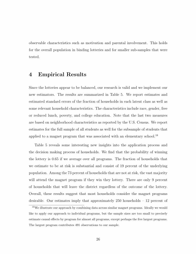
4 Empirical Results

Since the lotteries appear to be balanced, our research is valid and we implement our

new estimators. The results are summarized in Table 5. We report estimates and

estimated standard errors of the fraction of households in each latent class as well as

some relevant household characteristics. The characteristics include race, gender, free

or reduced lunch, poverty, and college education. Note that the last two measures

are based on neighborhood characteristics as reported by the U.S. Census. We report

estimates for the full sample of all students as well for the subsample of students that

applied to a magnet program that was associated with an elementary school.18

Table 5 reveals some interesting new insights into the application process and

the decision making process of households. We find that the probability of winning

the lottery is 0.65 if we average over all programs. The fraction of households that

we estimate to be at risk is substantial and consist of 19 percent of the underlying

population. Among the 73 percent of households that are not at risk, the vast majority

will attend the magnet program if they win they lottery. There are only 9 percent

of households that will leave the district regardless of the outcome of the lottery.

Overall, these results suggest that most households consider the magnet programs

desirable. Our estimates imply that approximately 250 households – 12 percent of

18We illustrate our approach by combining data across similar magnet programs. Ideally we would

like to apply our approach to individual programs, but the sample sizes are too small to precisely

estimate causal effects by program for almost all programs, except perhaps the five largest programs.

The largest program contributes 491 observations to our sample.

26

Table 5: Empirical Results

All Schools Elementary Schools

Coefficient Std. Error Coefficient Std. Error

Win 0.65 0.01 0.56 0.02

Fraction At Risk 0.19 0.02 0.22 0.03

Stay Attend Magnet 0.64 0.02 0.59 0.03

Stay-Non Magnet 0.09 0.01 0.07 0.01

Leave 0.09 0.01 0.12 0.01

At Risk 0.58 0.05 0.46 0.06

Black Stay-Magnet 0.81 0.01 0.69 0.03

Stay-Non Magnet 0.67 0.04 0.31 0.08

Leave 0.43 0.04 0.28 0.06

At Risk 0.55 0.05 0.60 0.07

Female Stay-Magnet 0.52 0.02 0.50 0.03

Stay-Non Magnet 0.53 0.05 0.52 0.09

Leave 0.37 0.04 0.39 0.06

At Risk 0.16 0.04 0.18 0.05

FRL Stay-Magnet 0.43 0.02 0.46 0.03

Stay-Non Magnet 0.26 0.04 0.29 0.08

Leave 0.08 0.02 0.05 0.03

At Risk 0.21 0.01 0.20 0.02

Poverty Stay-Magnet 0.24 0.01 0.24 0.01

Stay-Non Magnet 0.23 0.01 0.18 0.02

Leave 0.15 0.01 0.12 0.01

27

Table 5: Empirical Results (cont.)

All Schools Elementary Schools

Coefficient Std. Error Coefficient Std. Error

At Risk 0.34 0.02 0.42 0.04

College Stay-Magnet 0.27 0.01 0.30 0.01

Stay-Non Magnet 0.32 0.02 0.41 0.04

Leave 0.38 0.02 0.40 0.04

# Observations 2268 905

the underlying sample – decided to stay in the district because they won the magnet

lottery.

Equally interesting are the characteristics of the households that are at risk. For

each characteristic, the differences across household types (at risk, leavers, stayers)

are statistically significant. We find that these households are on average less likely

to be African American and on free or reduced lunch programs than households that

are stayers. Moreover, they come from more affluent and better educated neigh-

borhoods.19 We thus conclude that magnet programs are effective devices for the

school district to retain more affluent households. Not surprisingly, the group that

are leavers are the most affluent group. These households may just apply to the

magnet programs as a back-up option in case their students should unexpectedly not

be admitted to an independent, charter, or parochial school.20

19Note that the differences in household characteristics are statistically significant from zero at all

conventional levels.20It could also be that these households left the district because of job transfers or other issues

unrelated to schools.

28

Table 5 also provides estimates when we restrict attention to households that

apply to programs that provide education for children in elementary school. These

programs are slightly more competitive as can be seen from the lower probability

of winning (0.56 versus 0.65). Moreover, these programs attract a more educated

clientele. The fraction of African American families is also lower in this subsample.

Not surprisingly, we find that the fraction of at risk families and the fraction of leavers

is also higher in this sample. This finding highlights the fact the market for elementary

school education is more competitive than the market for high school education.

Table 6: Ability Sorting

High Schools

Coefficient Std. Error

Win 0.86 0.01

Fraction At Risk 0.06 0.04

Stay Attend Magnet 0.83 0.04

Stay-Non Magnet 0.06 0.01

Leave 0.05 0.01

At Risk 1399 169

Math Stay-Magnet 1261 13

Stay-Non Magnet 1262 45

Leave 1347 45

At Risk 1380 165

Reading Stay-Magnet 1299 16

Stay-Non Magnet 1238 42

Leave 1413 56

# Observations 530

29

Finally, we consider the results for high school applicants. This sub-sample is

interesting since we observe test scores for all students in these subsample. We can

thus analyze sorting based on ability measured by prior test scores. We implement

our GMM estimator using the full set of observed characteristics. In Table 6. we

only report the results that pertain to attraction and retention as well as to sorting

by ability.21

Results are reported in Table 6. We find that the fraction of households that are

at risk and leavers are much smaller than in the full sample. Overall Table 6 provides

some evidence in favor of ability sorting. Households that are considered to be at

risk have on average children with higher math and reading test scores. Households

that stay in the district regardless of the outcome of the lottery have the lower test

scores. We thus conclude that magnet program retain higher ability students who

would leave the district in the absence of these programs.

5 Conclusions

We have considered a research design in which program participation is only partially

determined by randomization. These designs arise when randomization occurs at the

application stage and potential participants that are randomized into the program

can always opt out before the program begins. These designs are commonly used to

determine access to oversubscribed program offered by public school systems. We have

developed a new empirical method which classifies potential participants in to stayers,

leavers, and those that are at risk. The last group of individuals are most interesting

form a policy perspective since the decision to participate crucially depends on the

outcome of the lottery. We have shown that the parameters that characterize the

causal effects are identified and can be estimated using a GMM estimator. Commonly

21The full set of results are available upon request from the authors.

30

applied IV and OLS estimators partially identify key components of our framework.

We have applied our new methods to study the effectiveness of magnet program in

attracting and retaining students and households in a large urban school district. Our

findings suggest that magnet programs are useful tools that help the district to attract

and retain students from middle class backgrounds. These households have many

options outside the public school system. It is considerably more difficult to study

the impact of these programs on achievement because of attrition and selection. Some

households that do not win the lottery decide to leave the district and pursue other

school options for their children. These households have very different observable

characteristics then the households that stay behind. It is therefore plausible to

assume that households also differ in unobserved characteristics. As a consequence,

our experimental design allows us to point identify and estimate the effects associated

with retention and attraction of students. For other treatment effects we can construct

informative bounds.

31

References

Abadie, A. and Imbens, G. (2006). Large Sample Properties of Matching Estimators for Average

Treatment Effects. Econometrica, 74 (1), 235–67.

Angrist, J. (1990). Lifetime Earnings and the Vietnam Era Draft Lottery: Evidence from Social

Security Administrative Records. American Economic Review, 80, 313–36.

Angrist, J., Bettinger, E., Bloom, E., King, E., and Kremer, M. (2002). Vouchers for Private

Schooling in Colombia: Evidence from a Randomized Natural Experiment. American Eco-

nomic Review, 92, 1535–58.

Angrist, J. and Imbens, G. (1994). Identification and Estimation of Local Average Treatment Effects.

Econometrica, 62 (2), 467–79.

Angrist, J., Imbens, G., and Rubin, D. (1996). Identification of Causal Effects Using Instrumental

Variables. Journal of the American Statistical Association, 91, 444–56.

Ballou, D., Goldring, E., and Liu, K. (2006). Magnet Schools and Student Achievement. Working

Paper.

Bjorklund, A. and Moffitt, R. (1987). The Estimation of Wage and Welfare Gains in Self-Selection

Models. Review of Economics and Statistics, 69, 42–49.

Cullen, J., Jacob, B., and Levitt, S. (2006). The Effect of School Choice on Student Outcomes:

Evidence From Randomized Lotteries. Econometrica, 74(5), 1191–230.

Durbin, J. (1954). Errors in Variables. Review of the International Statistical Institute, 22, 23–32.

Fisher, R. (1935). Design of Experiments. Hafner. New York.

Hansen, L. P. (1982). Large Sample Properties of Generalized Method of Moments Estimators.

Econometrica, 50 (4), 1029–1053.

Hastings, J., Kane, T., and Staiger, D. (2006). Paternal Preferences and School Competition:

Evidence from a Public School Choice Program. Working Paper.

Heckman, J. (1978). Dummy Endogenous Variables in a Simultaneous Equation System. Econo-

metrica, 46, 931–960.

Heckman, J. (1979). Sample Selection Bias as a Specification Error. Econometrica, 47 (1), 153–161.

32

Heckman, J. and Honore, B. (1990). The Empirical Content of the Roy Model. Econometrica, 58

(5), 1121–49.

Heckman, J., Ichimura, H., and Todd, P. (1997). Matching As An Econometric Evaluation Estimator:

Evidence from Evaluating a Job Training Program. Review of Economic Studies, 64 (4).

Heckman, J. and Robb, R. (1985). Alternative Methods for Evaluating the Impact of Interventions.

In Longitudinal Analysis of Labor Market Data. Cambridge University Press.

Heckman, J. and Vytlacil, E. (2005). Structural Equations, Treatment Effects and Econometric

Policy Evaluation. Econometrica, 73.

Heckman, J. and Vytlacil, E. (2007). Econometric Evaluation of Social Programs. In Handbook of

Econometrics 6b. Elsevier North Holland.

Hoxby, C. and Rockoff, J. (2004). The Impact of Charter Schools on Student Achievement. Working

Paper.

Kim, S. (1992). A Practical Solution to the Multivariate Behrens-Fisher Problem. Biometrica, 79,

171–6.

Lee, L. (1979). Identification and Estimation in Binary Choice Models with Limited (Censored)

Dependent Variables. Econometrica, 47, 977–996.

Maddala, G. (1983). Limited Dependent and Qualitative Response Variables in Econometrics. Cam-

bridge University Press.

Moffitt, R. (2008). Estimating Marginal Treatment Effects in Heterogeneous Populations. Working

Paper.

Quandt, R. (1972). A New Approach to Estimating Switching Regression Models. Journal of the

American Statistical Association, 67, 306–310.

Rosenbaum, P. and Rubin, D. (1983). The central role of the propensity score in observational

studies for causal effects. Biometrica, 70, 41–55.

Rouse, C. (1998). Private School Vouchers and Student Achievement: An Evaluation of the Mil-

waukee Parental Choice Program. Quarterly Journal of Economics, 113, 553–602.

Rubin, D. (1974). Estimating Causal Effects of Treatment in Randomized and Nonrandomized

Studies. Journal of Educational Psychology, 66, 688–701.

Rubin, D. (1978). Bayesian Inference For Causal Effects. Annals of Statistics, 6, 34–58.

33