Estimation of Atmospheric Motion Vectors from Kalpana-1 Imagers

Estimation of Atmospheric Motion Vectors from Kalpana-1 Imagers

C. M. KISHTAWAL, S. K. DEB, P. K. PAL, AND P. C. JOSHI

Atmospheric Sciences Division, Meteorology and Oceanography Group, Remote Sensing Applications Area,

Space Applications Centre, ISRO, Ahmedabad, India

(Manuscript received 19 November 2008, in final form 2 June 2009)

ABSTRACT

The estimation of atmospheric motion vectors from infrared and water vapor channels on the geostationary

operational Indian National Satellite System Kalpana-1 has been attempted here. An empirical height as-

signment technique based on a genetic algorithm is used to determine the height of cloud and water vapor

tracers. The cloud-motion-vector (CMV) winds at high and midlevels and water vapor winds (WVW) derived

from Kalpana-1 show a very close resemblance to the corresponding Meteosat-7 winds derived at the

European Organisation for the Exploitation of Meteorological Satellites when both are compared separately

with radiosonde data. The 3-month mean vector difference (MVD) of high- and midlevel CMV and WVW

winds derived from Kalpana-1 is very close to that of Meteosat-7 winds, when both are compared with ra-

diosonde. When comparing with radiosonde, the low-level CMVs from Kalpana-1 have a higher MVD value

than that of Meteosat-7. This may be due to the difference in spatial resolutions of Kalpana-1 and Meteosat-7.

1. Introduction

During the 1970s and early 1980s, satellite winds were

produced using a combination of automated and manual

techniques (Leese et al. 1971; Young 1975). The oper-

ational derivation of atmospheric motion vectors such

as cloud-motion vector (CMV) and water vapor winds

(WVW) from infrared and water vapor channels of

three successive geostationary satellite images started in

the early 1970s (Fujita 1968; Hubert and Whitney 1971).

The uses of geostationary water vapor imagery have

allowed the determination of upper-level moisture

content and winds in cloud-free regions as well. Fur-

thermore, for the last decade the extraction of atmo-

spheric motion vectors from satellite images [like IR

and water vapor (WV)] has become an important com-

ponent for operational numerical weather prediction

(NWP). With the advancement of different numerical

weather prediction and data assimilation techniques at

different operational centers, a significant contribution

of both middle and upper-air wind information is de-

rived from satellite observations that use the movement

of cloud and water vapor tracers to determine winds

operationally several times per day. These satellite wind

products, assimilated in both regional- and global-scale

models, result in positive impacts on weather forecasts

(Kelly 2004; Bedka and Mecikalski 2005), especially

over the tropics. The substantial works related to the

derivation of operational satellite winds and their im-

pacts in numerical weather prediction are currently

available from the Geostationary Operational Envi-

ronmental Satellite (GOES) series (Nieman et al. 1997;

Velden et al. 1997), the European Meteosat series

(Schmetz et al. 1993), and the Japanese Geostationary

Meteorological Satellite series (Tokuno 1996). However,

not much work has been done for wind retrieval from the

meteorological geostationary Indian National Satellite

System (INSAT) series (e.g., INSAT-3A, Kaplana-1). In

this study, an attempt has been made to derive the at-

mospheric motion vectors operationally using the data

from these INSAT platforms. With the availability of

IR-window (10.5 mm) and WV (6.3 mm) channels on the

Kalpana-1 Very High Resolution Radiometer (VHRR),

an attempt has been made here to derive cloud-tracked

winds (900–100 hPa) and WV winds (500–100 hPa) from

INSAT images. Sections 2 and 3 briefly summarize the

retrieval technique of winds from IR and WV channels.

The method for validating the retrieved winds and

Corresponding author address: Dr. S. K. Deb, Atmospheric

Sciences Division, Meteorology and Oceanography Group, Remote

Sensing Applications Area, Space Applications Centre, Indian

Space Research Organisation, Ahmedabad 380015, India.

E-mail: [email protected]

2410 J O U R N A L O F A P P L I E D M E T E O R O L O G Y A N D C L I M A T O L O G Y VOLUME 48

DOI: 10.1175/2009JAMC2159.1

� 2009 American Meteorological Society

verification results are given in section 4. Section 5

summarizes the conclusions from this study.

2. Algorithm for cloud-motion winds retrieval

The schematic diagram shown in Fig. 1a summarizes

the procedure for the detection of CMV winds using

Kalpana-1 IR data. Three consecutive images at 30-min

intervals are used to determine the CMVs. The follow-

ing steps are involved in this process: 1) image ‘‘thresh-

olding,’’ 2) feature selection and tracking for CMV

extraction, 3) use of image triplet and basic quality

control, and 4) height assignment. These steps are briefly

described below.

a. Image thresholding

Gray-level threshold values (GV) are predetermined

for the identification of land/ocean, low-level clouds

(900–700 hPa), and high-level clouds (100–300 hPa).

These values were determined by histogram analysis of

a large number of images (Prasad et al. 2004). Threshold

values for inverted IR images (10 bit) are fixed as fol-

lows: if GV # 520 then it is land/ocean and no vector is

extracted, if 521 # GV # 640 then it is low clouds, and if

641 # GV # 880 then it is high clouds.

b. Feature selection and tracking for CMVextraction

At the National Environmental Satellite, Data, and

Information Service (NESDIS), the initial features are

selected by locating the highest pixel brightness values

for each target domain and computing the local gradients

around those locations (Nieman et al. 1997). Any gra-

dients greater than 158K are assigned as target locations,

and prospective targets also undergo a spatial coherence

analysis (Coakley and Bretherton 1982) to filter out un-

wanted targets. At the European Organisation for the

Exploitation of Meteorological Satellites (EUMETSAT),

the tracers in the Meteosat (first-generation satellites)

images are selected using multispectral histogram analysis

(Tomassini 1981), which extracts the dominating scenes

in an image segment corresponding to the area of 32 3

32 IR pixels or about 160 km 3 160 km at the sub-

satellite point. Later the selected templates undergo a

spatial coherence technique (Coakley and Bretherton

1982) to filter the image, to enhance the upper-level

cloud. Because the spatial resolution of the infrared

channel of Kalpana-1 (8 km) is coarser relative to GOES

(5 km) or Meteosat-7 (5 km), we used a 20 3 20 window

(called a template) to identify features in Kalpana-1

images. The maximum and average GV of a template are

used to determine the ‘‘class’’ of the template (e.g., low

cloud/high cloud). Further, if the distribution of gray

levels is ‘‘coherent’’ within a template, it is assumed that

it does not contain a traceable feature, and such tem-

plates are rejected. Coherence is measured in terms of

the variance of GV within the template. If a traceable

feature is found in the first image, the match of this

template is searched in the second image within a

‘‘search window’’ of 64 3 64 pixels, centered at the same

point as the template window. The 20 3 20 template in

the second image that lies within the search window

should have the same class as the template in the first

image; otherwise the template in the second window is

rejected.

The matching is done using the ‘‘cross correlation’’

(CC) method (Schmetz et al. 1993), in which the CC is

defined as

CC 5� [g(i, j)� g][h(i, j)� h]

sgs

h

, (1)

where g and h represent the spatial distribution of

GV in the first and second image templates, respec-

tively, overbars denote spatial averaging, and s is the

standard deviation of GV. Templates with CC , 0.8 are

rejected. The center of the template with the maximum

value of CC is considered to be the location of the

feature in the second image. This is the first set of the

motion vector for the given template location. Then

the template is shifted in the x and y directions and the

motion vectors are determined using the procedure

given above.

c. Use of image triplet and basic quality control

The step described in section 2b is repeated for the

second and third IR images, and a second set of motion

vectors is generated. In both of the above sets of CMVs

there are several vectors that are spurious. This may be

due to several factors. For example, clouds may not al-

ways act as rigid bodies. Some clouds may dissipate, and

other clouds may form. Also, with atmospheric motion,

clouds may change shape, and maximum correlation

may appear at some false location. Some rectification of

this problem can be done using basic quality-control

measures. The quality check is generally based on vector

acceleration checks and simple threshold techniques

that compare the derived vectors with their surrounding

vectors or with collocated forecast fields. All vectors that

show unrealistic retrievals or speed and directional de-

viations with respect to the surroundings by larger than

a predefined value are rejected. In this study, we have

employed the automatic quality-control procedure used

at EUMETSAT (Holmlund 1998). A brief description is

given in appendix A.

NOVEMBER 2009 N O T E S A N D C O R R E S P O N D E N C E 2411

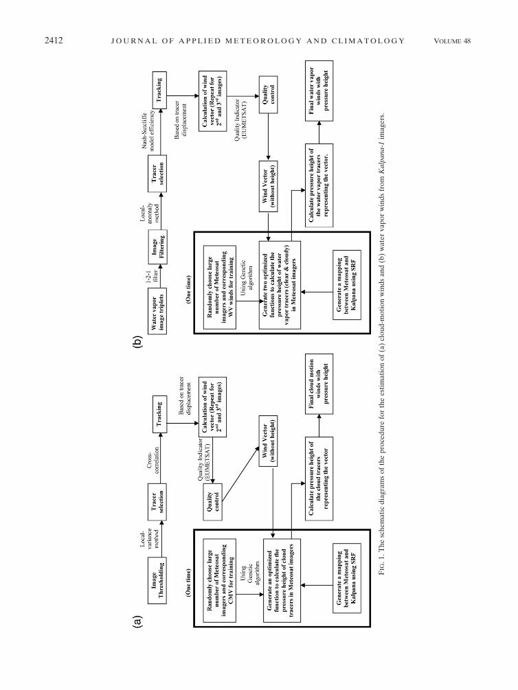
FIG

.1

.T

he

sch

ema

tic

dia

gra

ms

of

the

pro

ced

ure

for

the

est

ima

tio

no

f(a

)cl

ou

d-m

oti

on

win

ds

an

d(b

)w

ate

rv

ap

or

win

ds

fro

mK

alp

an

a-1

ima

gers

.

2412 J O U R N A L O F A P P L I E D M E T E O R O L O G Y A N D C L I M A T O L O G Y VOLUME 48

d. Height assignment

The old method of assigning heights to cloud-motion

winds is the infrared-window sampling (Fritz and

Winston 1962) method. In this method the window-

channel brightness temperatures (BT) within the target

area and a mean value for the coldest 20% of the sample

were used to represent the temperature at cloud top.

Later, this temperature was compared with a numerical

forecast of the vertical temperature profile to arrive at

the height of the cloud. Although this method had se-

rious problems in determining the heights of semi-

transparent cirrus (Menzel et al. 1983), it remains

a credible backup method in the current automated

processing scheme when the more sophisticated height-

assignment methods fail to deliver the correct height.

The carbon dioxide (CO2) slicing algorithm (Menzel

et al. 1983) remains the most accurate and dependable

means of assigning heights to semitransparent tracers

(Nieman et al. 1993). As derived by Smith et al. (1970),

the ratio of the deviations in observed radiances and the

corresponding clear-air radiances for the IR and CO2

absorption bands viewing the same field of view can be

expressed in terms of cloud amount, emissivity for ice

cloud, and the Planck blackbody radiance for opaque

cloud. Planck blackbody radiance can also be a function

of cloud-top pressure. Because the emissivities are ap-

proximately equal for the IR and CO2 channels, clear-

sky radiances are computed from the radiative transfer

equation and a numerical forecast of the vertical tem-

perature and moisture profiles, which are then used to

calculate the cloud-top pressure. This method is very

successful in computing the cloud tracer’s height in

GOES-7 data, most of the time (Nieman et al. 1997). If

the satellite is lacking a CO2-absorption channel, the

H2O-intercept algorithm (Schmetz et al. 1993) becomes

the best method for calculating the height of semi-

transparent cloud tracers. Comparisons of the two

methods have demonstrated that the H2O-intercept al-

gorithm is an adequate replacement (Nieman et al.

1993), especially for upper-level tracers. The algorithm

is based on the fact that the radiances from a single-level

cloud layer for two spectral bands vary linearly with

cloud amount. Radiances from the IR window and H2O

absorption bands are measured and compared with

Planck blackbody radiances as a function of cloud-top

pressure. A numerical forecast of temperature and hu-

midity profiles in the region is used for the necessary

radiative transfer calculations. Measured and calculated

radiances should agree for clear-sky and opaque cloud

conditions. The cloud-top height is inferred from the

linear extrapolation of measured radiances onto the

calculated curve of opaque cloud radiance.

However, for this study and for the first time, an em-

pirically derived height assignment technique based on

a genetic algorithm (GA) is developed and tested. A

very short description of the GA is given in appendix B.

A number of studies have been reported using GA for

the prediction of space–time variability of the sea sur-

face temperature (Alvarez et al. 2000), estimation of

surface heat fluxes (Singh et al. 2006), and monthly

mean air-sea temperature differences (Singh et al. 2005)

from satellite observations. In this study, an attempt has

been made to use this empirical approach to determine

the height of the cloud tracers.

The development of the retrieval algorithm for the es-

timation of cloud-tracer height involves a number of steps.

In the first step, a number of independent variables from

the imagers such as brightness temperature of the coldest

pixel, warmest pixel, cosine of latitude and zenith angle

information of the center of the template window, and so

on are considered in a large set of possible parameters. In

the second step we choose randomly a large number of

Meteosat-5 IR images and corresponding cloud-motion

winds derived by EUMETSAT from a 1-month (October

2006) period as the training/validation dataset. Approxi-

mately 120 000 valid wind vectors were available in the

above dataset, but only 20% of the data were further se-

lected randomly for the purpose of training, and the re-

maining data were used for validation. A small ratio of

training and validation data size is expected to ensure the

robustness of the retrieved functions and also prevents the

possibility of overfitting. A 20 3 20 template window was

considered to be ‘‘cloudy’’ if the average brightness tem-

perature of the 25 coldest pixels was less than 220 K. The

GA is an automatic method that determines the most

fitting relationship between dependent and independent

fields using a random search and optimization criteria. In

this case, the optimized GA solution retains only the

following independent parameters that are needed for

height assignment of a tracer: 1) average BT of the 25

coldest pixels, 2) average BT of the 25 warmest pixels, and

3) cosine of latitude at the center of the template window.

One advantage of the GA method is that the complex and

often nonlinear relations can be obtained in functional

forms that are easier to use than lookup tables. Later, a

mapping was defined between Meteosat-5 and Kalpana-1

using the sensor response function (SRF) of both satellites

so that the function generated using Meteosat-5 can be

used in Kalpana-1 CMVs. Last, these functions for cloud

tracers are used to find the tracer height in Kalpana-1

through the mapping. The tracer heights derived by the

above method are in hectopascals. The current GA-based

approach is an ad hoc method and tries to mimic

statistically the operational height assignment method

used in Meteosat-5, which has its own limitations. A

NOVEMBER 2009 N O T E S A N D C O R R E S P O N D E N C E 2413

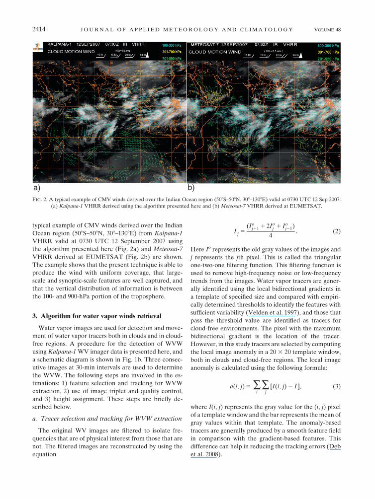
typical example of CMV winds derived over the Indian

Ocean region (508S–508N, 308–1308E) from Kalpana-1

VHRR valid at 0730 UTC 12 September 2007 using

the algorithm presented here (Fig. 2a) and Meteosat-7

VHRR derived at EUMETSAT (Fig. 2b) are shown.

The example shows that the present technique is able to

produce the wind with uniform coverage, that large-

scale and synoptic-scale features are well captured, and

that the vertical distribution of information is between

the 100- and 900-hPa portion of the troposphere.

3. Algorithm for water vapor winds retrieval

Water vapor images are used for detection and move-

ment of water vapor tracers both in clouds and in cloud-

free regions. A procedure for the detection of WVW

using Kalpana-1 WV imager data is presented here, and

a schematic diagram is shown in Fig. 1b. Three consec-

utive images at 30-min intervals are used to determine

the WVW. The following steps are involved in the es-

timations: 1) feature selection and tracking for WVW

extraction, 2) use of image triplet and quality control,

and 3) height assignment. These steps are briefly de-

scribed below.

a. Tracer selection and tracking for WVW extraction

The original WV images are filtered to isolate fre-

quencies that are of physical interest from those that are

not. The filtered images are reconstructed by using the

equation

Ij5

(Ioj11 1 2Io

j 1 Ioj�1)

4. (2)

Here Io represents the old gray values of the images and

j represents the jth pixel. This is called the triangular

one-two-one filtering function. This filtering function is

used to remove high-frequency noise or low-frequency

trends from the images. Water vapor tracers are gener-

ally identified using the local bidirectional gradients in

a template of specified size and compared with empiri-

cally determined thresholds to identify the features with

sufficient variability (Velden et al. 1997), and those that

pass the threshold value are identified as tracers for

cloud-free environments. The pixel with the maximum

bidirectional gradient is the location of the tracer.

However, in this study tracers are selected by computing

the local image anomaly in a 20 3 20 template window,

both in clouds and cloud-free regions. The local image

anomaly is calculated using the following formula:

a(i, j) 5 �i

�j

[I(i, j)� I ], (3)

where I(i, j) represents the gray value for the (i, j) pixel

of a template window and the bar represents the mean of

gray values within that template. The anomaly-based

tracers are generally produced by a smooth feature field

in comparison with the gradient-based features. This

difference can help in reducing the tracking errors (Deb

et al. 2008).

FIG. 2. A typical example of CMV winds derived over the Indian Ocean region (508S–508N, 308–1308E) valid at 0730 UTC 12 Sep 2007:

(a) Kalpana-1 VHRR derived using the algorithm presented here and (b) Meteosat-7 VHRR derived at EUMETSAT.

2414 J O U R N A L O F A P P L I E D M E T E O R O L O G Y A N D C L I M A T O L O G Y VOLUME 48

The cross-correlation technique is used operationally

for tracking the tracer between two WV images in most

operational centers. However, in this study the degrees

of matching between two successive images are calcu-

lated by the Nash–Sutcliffe model efficiency (Nash and

Sutcliffe 1970) coefficient E. It is defined as

E 5 1��

n

i51(I

t� I

s)2

�n

i51(I

t� I

t)2

, (4)

where It and Is are the variance of the gray values for the

template window and search window and It is the aver-

age of variance of the template window. Here n 5 20 3

20 is the size of the template window and corresponding

template of the same size in the searching area. The size

of the searching area in the subsequent image is taken as

64 3 64. The coefficient E is normalized to values be-

tween 2‘ and 11. An efficiency E 5 1 corresponds to a

perfect match, E 5 0 means that the search window is as

accurate as the mean of the template window, and E , 0

implies a lack of matching between the template and

search window. The closer the model efficiency is to 1,

the more accurate is the matching between the windows.

A cutoff value of E 5 0.8 is defined, below which a

matching of target is not considered. Toward the higher

end (e.g., as E / 1.0), the value of E approaches r2,

where r is the correlation coefficient. Thus a value of E 5 1

is exactly equivalent to a correlation of 1.0 between two

objects. The maximum value of E is chosen as the best fit

for tracking. One of the main advantages of this match-

ing technique is that it reduces the possibility of multiple

maxima, because the parameter E has a higher sensitivity

to differences between two features when compared with

the maximum cross-correlation coefficient (MCC). Thus,

when the degree of mismatch between two objects in-

creases, the value of E falls more sharply when compared

with that of MCC, making E a better index for matching

two objects. The application of this tracking method in

the estimation of WVW using Meteosat-5 images has

shown some improvement over the Indian Ocean region

(Deb et al. 2008).

b. Use of image triplet and basic quality control

The previous step in section 3a is repeated for the

second and third WV images, and a second set of motion

vectors is generated. In both the above sets of WVWs

there are several vectors that are spurious, and rectifi-

cation of this problem is done using the automatic quality-

control procedure used at EUMETSAT (Holmlund 1998).

This technique is used for quality control of CMV winds

using infrared images and is discussed in appendix A.

c. Height assignment

The height assignment of WVW is a long-standing

problem. In cloud-free regions, the radiometric signal

from pure WV structure is a result of emittance over

a finite layer and is further complicated by the radiance

contributions from multiple moist layers (Weldon and

Holmes 1991). The challenge is to assign a height that

best represents the motion of the moisture feature. The

most common height assignment technique for water

vapor tracers is to take the effective brightness tem-

perature and assess the height at which displacement of

the tracers is attributed (Velden et al. 1997). In this

method, the brightness temperature of the target box is

averaged and matched with a collocated model guess

temperature profile and the level of optimum fit is then

used to assign the initial pressure height. This pressure

height is then corrected with 3D objective analysis using

a recursive filter (Hayden and Purser 1995). This method

is currently operational at NESDIS. At EUMETSAT,

the clear-sky WVW available with a 160-km resolution

are derived from the Meteosat satellites using the single-

level height assignment based on the cluster equivalent

blackbody temperature method. Another method based

on the WV contribution function calculated from a ra-

diative transfer model was also used to calculate the WV

tracer’s height (Rattenborg and Holmlund 1996).

As discussed in detail in section 2d and in appendix B,

the GA-based empirical technique was also used to

determine the height of the WV tracers. In the first step,

a number of independent variables from the imagers

such as BT of the coldest pixel, BT of the warmest pixel,

cosine of latitude, zenith angle information of the cen-

ter of template window, and so on are considered in

a large set of possible parameters. In the second step we

choose randomly a large number of Meteosat-5 WV

images and corresponding water vapor winds derived

by EUMETSAT from a 1-month (October 2006) period

as the training/validation dataset. After successful train-

ing, separate optimized functions were generated for

cloudy and noncloudy scenes (templates). Like in sec-

tion 2d, the optimized GA solution retains 1) an average

BT of the 25 coldest pixels, 2) an average BT of the 25

warmest pixels, and 3) the cosine of latitude at the center

of the template window as independent parameters for

height assignment. However, the form of the function

changes from cloudy to noncloudy tracers in WV images

(Deb et al. 2008). Later a mapping is defined between

Meteosat-5 and Kalpana-1 using SRF of both satellites

so that the function generated using Meteosat-5 can be

used in Kalpana-1 WVW. Last, the functions for cloudy

and noncloudy regions are used to find the WV tracer

heights in Kalpana-1 through the mapping. The current

NOVEMBER 2009 N O T E S A N D C O R R E S P O N D E N C E 2415

GA-based approach is an ad hoc method and tries to

statistically mimic the operational height assignment

method used in Meteosat-5, which has its own lim-

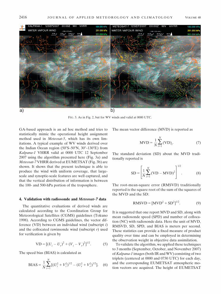
itations. A typical example of WV winds derived over

the Indian Ocean region (508S–508N, 308–1308E) from

Kalpana-1 VHRR valid at 0000 UTC 12 September

2007 using the algorithm presented here (Fig. 3a) and

Meteosat-7 VHRR derived at EUMETSAT (Fig. 3b) are

shown. It shows that the present technique is able to

produce the wind with uniform coverage, that large-

scale and synoptic-scale features are well captured, and

that the vertical distribution of information is between

the 100- and 500-hPa portion of the troposphere.

4. Validation with radiosonde and Meteosat-7 data

The quantitative evaluations of derived winds are

calculated according to the Coordination Group for

Meteorological Satellites (CGMS) guidelines (Tokuno

1998). According to CGMS guidelines, the vector dif-

ference (VD) between an individual wind (subscript i)

and the collocated rawinsonde wind (subscript r) used

for verification is given by

VD 5 [(Ui�U

r)2

1 (Vi� V

r)2]1/2. (5)

The speed bias (BIAS) is calculated as

BIAS 51

N�N

i51[(U2

i 1 V2i )1/2 � (U2

r 1 V2r )1/2]. (6)

The mean vector difference (MVD) is reported as

MVD 51

N�N

i51(VD)

i. (7)

The standard deviation (SD) about the MVD tradi-

tionally reported is

SD 51

N�N

i51(VD�MVD)2

24

35

1/2

. (8)

The root-mean-square error (RMSVD) traditionally

reported is the square root of the sum of the squares of

the MVD and the SD:

RMSVD 5 [MVD2 1 SD2]1/2. (9)

It is suggested that one report MVD and SD, along with

mean radiosonde speed (SPD) and number of colloca-

tion (NC) with radiosonde data. Here the unit of MVD,

RMSVD, SD, SPD, and BIAS is meters per second.

These statistics can provide a fixed measure of product

quality over time and can be employed in determining

the observation weight in objective data assimilation.To validate the algorithm, we applied these techniques

to 3 months (September, October, and November 2007)

of Kalpana-1 images (both IR and WV) consisting of two

triplets (centered at 0000 and 0730 UTC) for each day,

and the corresponding EUMETSAT atmospheric mo-

tion vectors are acquired. The height of EUMETSAT

FIG. 3. As in Fig. 2, but for WV winds and valid at 0000 UTC.

2416 J O U R N A L O F A P P L I E D M E T E O R O L O G Y A N D C L I M A T O L O G Y VOLUME 48

winds is derived by EUMETSAT height-assignment

techniques. The derived CMVs as well as WVWs obtained

by the present algorithm from Kalpana-1 and corre-

sponding EUMETSAT winds (derived at EUMETSAT

using Meteosat-7) are compared with collocated radio-

sonde for each day by calculating different statistical

parameters as discussed above for the region 508N–508S

and 308–1308E. During collocation, the nearest radio-

sonde and retrieved winds within a 18 3 18 grid box are

compared. Levelwise error statistics were then gener-

ated (high, mid-, and low levels) according to the CGMS

guidelines. The points for which either the difference

of speed between retrieved and radiosonde winds was

more than 30 m s21 or the difference of direction was

more than 908 were considered to be erroneous points

(due either to wrong retrieval or to errors in radiosonde

observation) and were filtered out from the validation

dataset. A total of around 5%–7% of cases lie beyond

this category, out of which 1%–2% are due to the speed

differences and the rest are due to directional differ-

ences for both satellites for this period of validation.

a. Cloud-motion winds

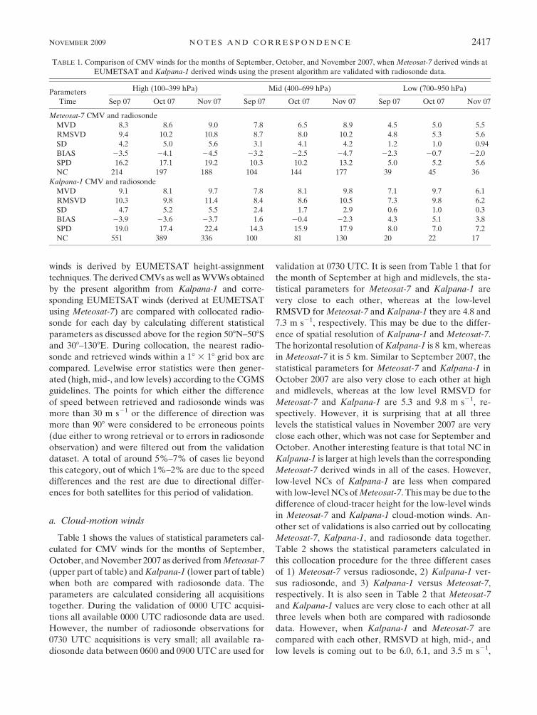
Table 1 shows the values of statistical parameters cal-

culated for CMV winds for the months of September,

October, and November 2007 as derived from Meteosat-7

(upper part of table) and Kalpana-1 (lower part of table)

when both are compared with radiosonde data. The

parameters are calculated considering all acquisitions

together. During the validation of 0000 UTC acquisi-

tions all available 0000 UTC radiosonde data are used.

However, the number of radiosonde observations for

0730 UTC acquisitions is very small; all available ra-

diosonde data between 0600 and 0900 UTC are used for

validation at 0730 UTC. It is seen from Table 1 that for

the month of September at high and midlevels, the sta-

tistical parameters for Meteosat-7 and Kalpana-1 are

very close to each other, whereas at the low-level

RMSVD for Meteosat-7 and Kalpana-1 they are 4.8 and

7.3 m s21, respectively. This may be due to the differ-

ence of spatial resolution of Kalpana-1 and Meteosat-7.

The horizontal resolution of Kalpana-1 is 8 km, whereas

in Meteosat-7 it is 5 km. Similar to September 2007, the

statistical parameters for Meteosat-7 and Kalpana-1 in

October 2007 are also very close to each other at high

and midlevels, whereas at the low level RMSVD for

Meteosat-7 and Kalpana-1 are 5.3 and 9.8 m s21, re-

spectively. However, it is surprising that at all three

levels the statistical values in November 2007 are very

close each other, which was not case for September and

October. Another interesting feature is that total NC in

Kalpana-1 is larger at high levels than the corresponding

Meteosat-7 derived winds in all of the cases. However,

low-level NCs of Kalpana-1 are less when compared

with low-level NCs of Meteosat-7. This may be due to the

difference of cloud-tracer height for the low-level winds

in Meteosat-7 and Kalpana-1 cloud-motion winds. An-

other set of validations is also carried out by collocating

Meteosat-7, Kalpana-1, and radiosonde data together.

Table 2 shows the statistical parameters calculated in

this collocation procedure for the three different cases

of 1) Meteosat-7 versus radiosonde, 2) Kalpana-1 ver-

sus radiosonde, and 3) Kalpana-1 versus Meteosat-7,

respectively. It is also seen in Table 2 that Meteosat-7

and Kalpana-1 values are very close to each other at all

three levels when both are compared with radiosonde

data. However, when Kalpana-1 and Meteosat-7 are

compared with each other, RMSVD at high, mid-, and

low levels is coming out to be 6.0, 6.1, and 3.5 m s21,

TABLE 1. Comparison of CMV winds for the months of September, October, and November 2007, when Meteosat-7 derived winds at

EUMETSAT and Kalpana-1 derived winds using the present algorithm are validated with radiosonde data.

Parameters High (100–399 hPa) Mid (400–699 hPa) Low (700–950 hPa)

Time Sep 07 Oct 07 Nov 07 Sep 07 Oct 07 Nov 07 Sep 07 Oct 07 Nov 07

Meteosat-7 CMV and radiosonde

MVD 8.3 8.6 9.0 7.8 6.5 8.9 4.5 5.0 5.5

RMSVD 9.4 10.2 10.8 8.7 8.0 10.2 4.8 5.3 5.6

SD 4.2 5.0 5.6 3.1 4.1 4.2 1.2 1.0 0.94

BIAS 23.5 24.1 24.5 23.2 22.5 24.7 22.3 20.7 22.0

SPD 16.2 17.1 19.2 10.3 10.2 13.2 5.0 5.2 5.6

NC 214 197 188 104 144 177 39 45 36

Kalpana-1 CMV and radiosonde

MVD 9.1 8.1 9.7 7.8 8.1 9.8 7.1 9.7 6.1

RMSVD 10.3 9.8 11.4 8.4 8.6 10.5 7.3 9.8 6.2

SD 4.7 5.2 5.5 2.4 1.7 2.9 0.6 1.0 0.3

BIAS 23.9 23.6 23.7 1.6 20.4 22.3 4.3 5.1 3.8

SPD 19.0 17.4 22.4 14.3 15.9 17.9 8.0 7.0 7.2

NC 551 389 336 100 81 130 20 22 17

NOVEMBER 2009 N O T E S A N D C O R R E S P O N D E N C E 2417

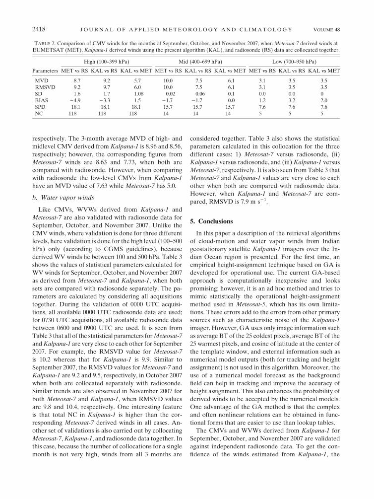
respectively. The 3-month average MVD of high- and

midlevel CMV derived from Kalpana-1 is 8.96 and 8.56,

respectively; however, the corresponding figures from

Meteosat-7 winds are 8.63 and 7.73, when both are

compared with radiosonde. However, when comparing

with radiosonde the low-level CMVs from Kalpana-1

have an MVD value of 7.63 while Meteosat-7 has 5.0.

b. Water vapor winds

Like CMVs, WVWs derived from Kalpana-1 and

Meteosat-7 are also validated with radiosonde data for

September, October, and November 2007. Unlike the

CMV winds, where validation is done for three different

levels, here validation is done for the high level (100–500

hPa) only (according to CGMS guidelines), because

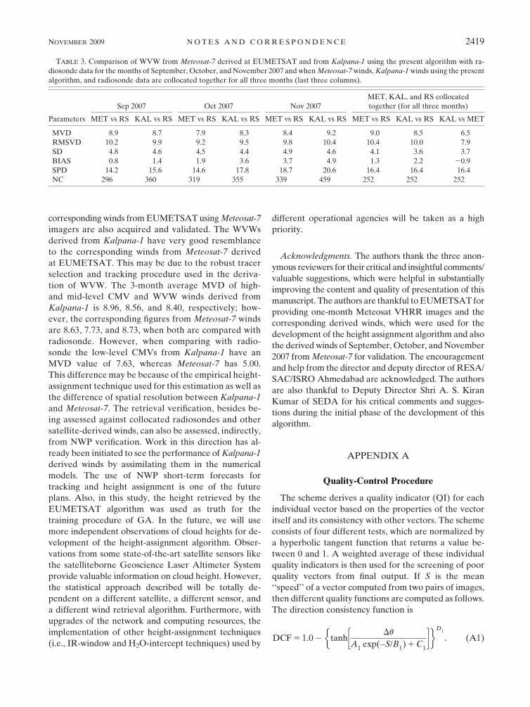
derived WV winds lie between 100 and 500 hPa. Table 3

shows the values of statistical parameters calculated for

WV winds for September, October, and November 2007

as derived from Meteosat-7 and Kalpana-1, when both

sets are compared with radiosonde separately. The pa-

rameters are calculated by considering all acquisitions

together. During the validation of 0000 UTC acquisi-

tions, all available 0000 UTC radiosonde data are used;

for 0730 UTC acquisitions, all available radiosonde data

between 0600 and 0900 UTC are used. It is seen from

Table 3 that all of the statistical parameters for Meteosat-7

and Kalpana-1 are very close to each other for September

2007. For example, the RMSVD value for Meteosat-7

is 10.2 whereas that for Kalpana-1 is 9.9. Similar to

September 2007, the RMSVD values for Meteosat-7 and

Kalpana-1 are 9.2 and 9.5, respectively, in October 2007

when both are collocated separately with radiosonde.

Similar trends are also observed in November 2007 for

both Meteosat-7 and Kalpana-1, when RMSVD values

are 9.8 and 10.4, respectively. One interesting feature

is that total NC in Kalpana-1 is higher than the cor-

responding Meteosat-7 derived winds in all cases. An-

other set of validations is also carried out by collocating

Meteosat-7, Kalpana-1, and radiosonde data together. In

this case, because the number of collocations for a single

month is not very high, winds from all 3 months are

considered together. Table 3 also shows the statistical

parameters calculated in this collocation for the three

different cases: 1) Meteosat-7 versus radiosonde, (ii)

Kalpana-1 versus radiosonde, and (iii) Kalpana-1 versus

Meteosat-7, respectively. It is also seen from Table 3 that

Meteosat-7 and Kalpana-1 values are very close to each

other when both are compared with radiosonde data.

However, when Kalpana-1 and Meteosat-7 are com-

pared, RMSVD is 7.9 m s21.

5. Conclusions

In this paper a description of the retrieval algorithms

of cloud-motion and water vapor winds from Indian

geostationary satellite Kalpana-1 imagers over the In-

dian Ocean region is presented. For the first time, an

empirical height-assignment technique based on GA is

developed for operational use. The current GA-based

approach is computationally inexpensive and looks

promising; however, it is an ad hoc method and tries to

mimic statistically the operational height-assignment

method used in Meteosat-5, which has its own limita-

tions. These errors add to the errors from other primary

sources such as characteristic noise of the Kalpana-1

imager. However, GA uses only image information such

as average BT of the 25 coldest pixels, average BT of the

25 warmest pixels, and cosine of latitude at the center of

the template window, and external information such as

numerical model outputs (both for tracking and height

assignment) is not used in this algorithm. Moreover, the

use of a numerical model forecast as the background

field can help in tracking and improve the accuracy of

height assignment. This also enhances the probability of

derived winds to be accepted by the numerical models.

One advantage of the GA method is that the complex

and often nonlinear relations can be obtained in func-

tional forms that are easier to use than lookup tables.

The CMVs and WVWs derived from Kalpana-1 for

September, October, and November 2007 are validated

against independent radiosonde data. To get the con-

fidence of the winds estimated from Kalpana-1, the

TABLE 2. Comparison of CMV winds for the months of September, October, and November 2007, when Meteosat-7 derived winds at

EUMETSAT (MET), Kalpana-1 derived winds using the present algorithm (KAL), and radiosonde (RS) data are collocated together.

High (100–399 hPa) Mid (400–699 hPa) Low (700–950 hPa)

Parameters MET vs RS KAL vs RS KAL vs MET MET vs RS KAL vs RS KAL vs MET MET vs RS KAL vs RS KAL vs MET

MVD 8.7 9.2 5.7 10.0 7.5 6.1 3.1 3.5 3.5

RMSVD 9.2 9.7 6.0 10.0 7.5 6.1 3.1 3.5 3.5

SD 1.6 1.7 1.08 0.02 0.06 0.1 0.0 0.0 0

BIAS 24.9 23.3 1.5 21.7 21.7 0.0 1.2 3.2 2.0

SPD 18.1 18.1 18.1 15.7 15.7 15.7 7.6 7.6 7.6

NC 118 118 118 14 14 14 5 5 5

2418 J O U R N A L O F A P P L I E D M E T E O R O L O G Y A N D C L I M A T O L O G Y VOLUME 48

corresponding winds from EUMETSAT using Meteosat-7

imagers are also acquired and validated. The WVWs

derived from Kalpana-1 have very good resemblance

to the corresponding winds from Meteosat-7 derived

at EUMETSAT. This may be due to the robust tracer

selection and tracking procedure used in the deriva-

tion of WVW. The 3-month average MVD of high-

and mid-level CMV and WVW winds derived from

Kalpana-1 is 8.96, 8.56, and 8.40, respectively; how-

ever, the corresponding figures from Meteosat-7 winds

are 8.63, 7.73, and 8.73, when both are compared with

radiosonde. However, when comparing with radio-

sonde the low-level CMVs from Kalpana-1 have an

MVD value of 7.63, whereas Meteosat-7 has 5.00.

This difference may be because of the empirical height-

assignment technique used for this estimation as well as

the difference of spatial resolution between Kalpana-1

and Meteosat-7. The retrieval verification, besides be-

ing assessed against collocated radiosondes and other

satellite-derived winds, can also be assessed, indirectly,

from NWP verification. Work in this direction has al-

ready been initiated to see the performance of Kalpana-1

derived winds by assimilating them in the numerical

models. The use of NWP short-term forecasts for

tracking and height assignment is one of the future

plans. Also, in this study, the height retrieved by the

EUMETSAT algorithm was used as truth for the

training procedure of GA. In the future, we will use

more independent observations of cloud heights for de-

velopment of the height-assignment algorithm. Obser-

vations from some state-of-the-art satellite sensors like

the satelliteborne Geoscience Laser Altimeter System

provide valuable information on cloud height. However,

the statistical approach described will be totally de-

pendent on a different satellite, a different sensor, and

a different wind retrieval algorithm. Furthermore, with

upgrades of the network and computing resources, the

implementation of other height-assignment techniques

(i.e., IR-window and H2O-intercept techniques) used by

different operational agencies will be taken as a high

priority.

Acknowledgments. The authors thank the three anon-

ymous reviewers for their critical and insightful comments/

valuable suggestions, which were helpful in substantially

improving the content and quality of presentation of this

manuscript. The authors are thankful to EUMETSAT for

providing one-month Meteosat VHRR images and the

corresponding derived winds, which were used for the

development of the height assignment algorithm and also

the derived winds of September, October, and November

2007 from Meteosat-7 for validation. The encouragement

and help from the director and deputy director of RESA/

SAC/ISRO Ahmedabad are acknowledged. The authors

are also thankful to Deputy Director Shri A. S. Kiran

Kumar of SEDA for his critical comments and sugges-

tions during the initial phase of the development of this

algorithm.

APPENDIX A

Quality-Control Procedure

The scheme derives a quality indicator (QI) for each

individual vector based on the properties of the vector

itself and its consistency with other vectors. The scheme

consists of four different tests, which are normalized by

a hyperbolic tangent function that returns a value be-

tween 0 and 1. A weighted average of these individual

quality indicators is then used for the screening of poor

quality vectors from final output. If S is the mean

‘‘speed’’ of a vector computed from two pairs of images,

then different quality functions are computed as follows.

The direction consistency function is

DCF 5 1.0� tanhDu

A1

exp(�S/B1) 1 C

1

� �� �D1

. (A1)

TABLE 3. Comparison of WVW from Meteosat-7 derived at EUMETSAT and from Kalpana-1 using the present algorithm with ra-

diosonde data for the months of September, October, and November 2007 and when Meteosat-7 winds, Kalpana-1 winds using the present

algorithm, and radiosonde data are collocated together for all three months (last three columns).

Sep 2007 Oct 2007 Nov 2007

MET, KAL, and RS collocated

together (for all three months)

Parameters MET vs RS KAL vs RS MET vs RS KAL vs RS MET vs RS KAL vs RS MET vs RS KAL vs RS KAL vs MET

MVD 8.9 8.7 7.9 8.3 8.4 9.2 9.0 8.5 6.5

RMSVD 10.2 9.9 9.2 9.5 9.8 10.4 10.4 10.0 7.9

SD 4.8 4.6 4.5 4.4 4.9 4.6 4.1 3.6 3.7

BIAS 0.8 1.4 1.9 3.6 3.7 4.9 1.3 2.2 20.9

SPD 14.2 15.6 14.6 17.8 18.7 20.6 16.4 16.4 16.4

NC 296 360 319 355 339 459 252 252 252

NOVEMBER 2009 N O T E S A N D C O R R E S P O N D E N C E 2419

The speed consistency function is

SCF 5 1.0� tanhDS

max(A2S, B

2) 1 C

2

� �� �D2

. (A2)

The vector consistency function is

VCF 5 1.0� tanhDV

max(A3S, B

3) 1 C

3

� �� �D3

. (A3)

In the above formulation, Du, DS, and DV represent

the difference of direction (in degrees), difference of

speed, and the length of the difference vector between

the first and second satellite wind component. Quanti-

ties AN, BN, CN, and DN are constants. The final quality

indicator of a wind vector is given as

QI 5w1 3 DCF 1 w2 3 SCF 1 w3 3 VCF

3.0. (A4)

All vectors with QI , 0.6 are rejected. The values of

the constants AN, BN, CN, and DN and the weights (w1,

w2, and w3) are assigned according to the procedure

used in the EUMETSAT (2005) report.

APPENDIX B

Genetic Algorithm: Basic Concept

The GA is one of the best techniques (Szpiro 1997;

Alvarez et al. 2000; Singh et al. 2006) to determine the

optimum relationship between the independent and

dependent parameters. The genetic algorithm is pro-

grammed to approximate the equation, in symbolic form,

that best describes the relationship between independent

and dependent parameters. The GA considers an initial

population of potential solutions that is subjected to an

evolutionary process, by selecting those equations (in-

dividuals) that best fit the data. The strongest strings

(made up from a combination of variables, real numbers,

and arithmetic operators) choose a mate for reproduction

whereas the weaker strings become extinct. The newly

generated population is subjected to mutations that

change fractions of information. The evolutionary steps

are repeated with the new generation. The process ends

after a number of generations, determined a priori by

the user.

Let p() be a smooth mapping function that explains

the relationship between a desired variable x and a set of

independent variables (a, b, c, d, e, . . .) so that

x 5 p(a, b, c, d, e, . . .). (B1)

First, for an amplitude function x, a set of candidate

equations for p() is randomly generated. An equation is

stored as a set of characters that define the independent

variables, a, b, c, d, e, and so on, in the above equation,

and four arithmetic operators (1, 2, 3, and /). A cri-

terion that measures how well the equation strings per-

form on a training set of the data is its fitness to the data,

defined as the sum of the squared differences between

data and the parameter derived from the equation

string. The equations with best fits are then selected to

exchange parts of the character strings between them

while the equations with less fits are discarded. Last,

a small percentage of the equation strings, single oper-

ators, and variables are mutated at random. The process

is repeated for a large number of times to improve the

fitness of the evolving equations. The fitness strength of

the best-scoring equation is defined as

R2 5 1� D2

S(x0� hx

0i)2

" #, (B2)

where D2 5 S(xc 2 x0)2, xc is the parameter value esti-

mated by the best scoring equation, x0 is the corre-

sponding ‘‘true’’ value, and hx0i is the mean of the true

values of x. Szpiro (1997) has shown the robustness of

the GA in forecasting the behavior of a one-dimensional

chaotic dynamical system.

REFERENCES

Alvarez, A., C. Lopez, M. Riera, E. Hernandez-Garcia, and

J. Tintore, 2000: Forecasting the SST space-time variability of

the Alboran Sea with genetic algorithms. Geophys. Res. Lett.,

27, 2709–2712.

Bedka, K. M., and J. R. Mecikalski, 2005: Application of satellite-

derived atmospheric motion vectors for estimating meso-scale

flows. J. Appl. Meteor., 44, 1761–1772.

Coakley, J., and F. Bretherton, 1982: Cloud cover from high-

resolution scanner data; detecting and allowing for partially

filled fields of view. J. Geophys. Res., 87, 4917–4932.

Deb, S. K., C. M. Kishtawal, P. K. Pal, and P. C. Joshi, 2008: A

modified tracer selection and tracking procedure to derive

winds using water vapor imagers. J. Appl. Meteor. Climatol.,

47, 3252–3263.

EUMETSAT, 2005: Wind vector automatic quality control

scheme. EUM/OPS/TEN/05/1747, 10 pp. [Available online

at http://www.eumetsat.int/Home/Main/Documentation/

Technical_and_Scientific_Documentation/Technical_Notes/

SP_1124282585834?l5en.]

Fritz, S., and J. S. Winston, 1962: Synoptic use of radiation mea-

surements from satellite TIROS-II. Mon. Wea. Rev., 90, 1–9.

Fujita, T., 1968: Present status of cloud velocity computations from

ATS-1 and ATS-3. COSPAR Space Res., 9, 557–570.

Hayden, C. M., and R. J. Purser, 1995: Recursive filter objective

analysis of meteorological fields: Applications to NESDIS

operational processing. J. Appl. Meteor., 34, 3–15.

2420 J O U R N A L O F A P P L I E D M E T E O R O L O G Y A N D C L I M A T O L O G Y VOLUME 48

Holmlund, K., 1998: The utilization of statistical properties of

satellite-derived atmospheric motion vectors to derive quality

indicators. Wea. Forecasting, 13, 1093–1104.

Hubert, L. F., and L. F. Whitney Jr., 1971: Wind estimation from

geostationary-satellite picture. Mon. Wea. Rev., 99, 665–672.

Kelly, G., 2004: Observing system experiments of all main data types

in the ECMWF operational system. Proc. Third WMO Work-

shop on the Impact of Various Observing Systems on Numerical

Weather Prediction, WMO Tech. Rep. 1228, Alpbach, Austria,

WMO, 32–36.

Leese, J. A., C. S. Novak, and B. B. Clark, 1971: An automated

technique for obtaining cloud motion from geosynchronous sat-

ellite data using cross correlation. J. Appl. Meteor., 10, 118–132.

Menzel, W. P., W. L. Smith, and T. R. Stewart, 1983: Improved

cloud motion vector and altitude assignment using VAS.

J. Climate Appl. Meteor., 22, 377–384.

Nash, J. E., and J. V. Sutcliffe, 1970: River flow forecasting through

conceptual models. Part I: A discussion of principles. J. Hy-

drol., 10, 282–290.

Nieman, S. J., J. Schmetz, and W. P. Menzel, 1993: A comparison of

several techniques to assign heights to cloud tracers. J. Appl.

Meteor., 32, 1559–1568.

——, W. P. Menzel, C. M. Hayden, D. D. Gray, S. Wanzong,

C. Velden, and J. Daniels, 1997: Fully automated cloud-drift

winds in NESDIS operations. Bull. Amer. Meteor. Soc., 78,

1121–1133.

Prasad, S., D. Singh, Y. V. Rama Rao, and V. R. Rao, 2004: Re-

trieval and validation of cloud motion vectors using infrared

data from KALPANA-1 Satellite. Proc. Seventh Int. Winds

Workshop, EUM P42, Helsinki, Finland, EUMETSAT, 61–70.

Rattenborg, M., and K. Holmlund, 1996: Operational wind

products from new Meteosat Ground Segment. Proc. Third

Int. Winds Workshop, EUM P18, Ascona, Switzerland,

EUMETSAT, 53–59.

Schmetz, J., K. Holmlund, J. Hoffman, B. Strauss, B. Mason,

V. Gaertner, A. Koch, and L. van de Berg, 1993: Operational

cloud-motion winds from Meteosat infrared images. J. Appl.

Meteor., 32, 1206–1225.

Singh, R., C. M. Kishtawal, and P. C. Joshi, 2005: Estimation of

monthly mean air-sea temperature from satellite observations

using genetic algorithm. Geophys. Res. Lett., 32, L02807,

doi:10.1029/2004GL021531.

——, ——, P. K. Pal, and P. C. Joshi, 2006: Surface heat fluxes over

global ocean exclusively from satellite observations. Mon.

Wea. Rev., 134, 965–980.

Smith, W. L., H. M. Woolf, and W. J. Jacob, 1970: A regression

method for obtaining real-time temperature and geopotential

height profiles from satellite spectrometer measurements and

its application to Nimbus-3 SIRS observations. Mon. Wea.

Rev., 98, 604–611.

Szpiro, G. G., 1997: Forecasting chaotic time series with genetic

algorithm. Phys. Rev., 55, 2557–2568.

Tokuno, M., 1996: Operational system for extracting cloud motion

and water vapor motion winds from GMS-5 image data. Proc.

Third Int. Winds Workshop, EUM P18, Ascona, Switzerland,

EUMETSAT, 21–30.

——, 1998: Collocation area for comparison of satellite winds and

radiosondes. Proc. Fourth Int. Winds Workshop, EUM P24,

Saanenmoser, Switzerland, EUMETSAT, 21–28.

Tomassini, C., 1981: Objective analysis of cloud fields. Proc. Sat-

ellite Meteorology of the Mediterranean, SP-159, Erice, Italy,

ESA, 73–78.

Velden, C. S., C. M. Hayden, S. J. Nieman, W. P. Menzel,

S. Wanzong, and J. S. Goerss, 1997: Upper-tropospheric winds

derived from geostationary satellite water vapor observations.

Bull. Amer. Meteor. Soc., 78, 173–195.

Weldon, R. B., and S. J. Holmes, 1991: Water vapor imagery: In-

terpretation and applications to weather analysis and fore-

casting. NOAA Tech Rep. NESDIS 67, 213 pp.

Young, M. T., 1975: The GOES wind operation. NOAA Tech.

Memo. NESS 64, U.S. Dept. of Commerce, Springfield, VA,

111–121.

NOVEMBER 2009 N O T E S A N D C O R R E S P O N D E N C E 2421