Estimating Time Demand Elasticities Under Rationing. Victoria Prowse Nu¢ eld College, New Road, Oxford, OX1 1NF, UK. victoria.prowse@nu¢ eld.ox.ac.uk Telephone: +44(0) 7761447346 Fax: +44(0) 1865 278621 October 14, 2004 Abstract A multivariate extension of the standard labour supply model in presented. In the multivariate time allocation model leisure is disaggregated into a number of non market activities including sports, volunteer work and home production. Using data from the 2000 UK Time Use Survey, a linear expenditure system is estimated, allowing corner solutions in the time allocated to market work and non market activities. The e/ects of children, age, gender and education are largely as expected. The unusually high wage elasticities are attributed to a combination of the functional form of the linear expenditure and the treatment of the zero observations. Key Words: Time use, Labour supply, Corner solutions, Simulation inference. JEL Classication: C15, C34, J22. I would like to thank Steve Bond, ValØrie Lechene, Neil Shephard and participants at an Institute for Fiscal Studies seminar, March 2004. This work has been supported by scholarships from the Journal of Applied Econometrics and the E.S.R.C, grant number PAT-030-2003-00229. 1

Welcome message from author
This document is posted to help you gain knowledge. Please leave a comment to let me know what you think about it! Share it to your friends and learn new things together.
Transcript

Estimating Time Demand Elasticities Under Rationing.
Victoria Prowse�
Nu¢ eld College, New Road, Oxford, OX1 1NF, UK.
victoria.prowse@nu¢ eld.ox.ac.uk
Telephone: +44(0) 7761447346
Fax: +44(0) 1865 278621
October 14, 2004
Abstract
A multivariate extension of the standard labour supply model in presented. In the
multivariate time allocation model leisure is disaggregated into a number of non market
activities including sports, volunteer work and home production. Using data from the 2000
UK Time Use Survey, a linear expenditure system is estimated, allowing corner solutions
in the time allocated to market work and non market activities. The e¤ects of children,
age, gender and education are largely as expected. The unusually high wage elasticities
are attributed to a combination of the functional form of the linear expenditure and the
treatment of the zero observations.
Key Words: Time use, Labour supply, Corner solutions, Simulation inference.
JEL Classi�cation: C15, C34, J22.
�I would like to thank Steve Bond, Valérie Lechene, Neil Shephard and participants at an Institute for Fiscal
Studies seminar, March 2004. This work has been supported by scholarships from the Journal of Applied
Econometrics and the E.S.R.C, grant number PAT-030-2003-00229.
1
Estimating Time Demand Elasticities Under Rationing
1 Introduction
In the standard labour supply model all non market time is aggregated into a single quantity,
leisure. In this paper, a multivariate extension of the standard labour supply model is presented.
In the multivariate time allocation model leisure is disaggregated into a number of di¤erent non
market activities including sports, volunteer work and home production.
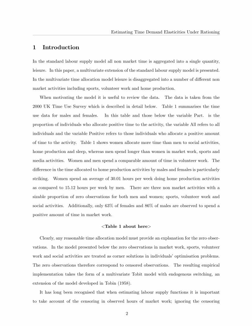
When motivating the model it is useful to review the data. The data is taken from the
2000 UK Time Use Survey which is described in detail below. Table 1 summarises the time
use data for males and females. In this table and those below the variable Part. is the
proportion of individuals who allocate positive time to the activity, the variable All refers to all
individuals and the variable Positive refers to those individuals who allocate a positive amount
of time to the activity. Table 1 shows women allocate more time than men to social activities,
home production and sleep, whereas men spend longer than women in market work, sports and
media activities. Women and men spend a comparable amount of time in volunteer work. The
di¤erence in the time allocated to home production activities by males and females is particularly
striking. Women spend an average of 30.01 hours per week doing home production activities
as compared to 15.12 hours per week by men. There are three non market activities with a
sizable proportion of zero observations for both men and women; sports, volunteer work and
social activities. Additionally, only 63% of females and 86% of males are observed to spend a
positive amount of time in market work.
<Table 1 about here>
Clearly, any reasonable time allocation model must provide an explanation for the zero obser-
vations. In the model presented below the zero observations in market work, sports, volunteer
work and social activities are treated as corner solutions in individuals�optimisation problems.
The zero observations therefore correspond to censored observations. The resulting empirical
implementation takes the form of a multivariate Tobit model with endogenous switching, an
extension of the model developed in Tobin (1958).
It has long been recognised that when estimating labour supply functions it is important
to take account of the censoring in observed hours of market work; ignoring the censoring
2

Estimating Time Demand Elasticities Under Rationing
in observed hours leads to biased and inconsistent estimates of the parameters of the labour
supply function (see Wales and Woodland, 1980). In the simplest case, censoring occurs when
desired hours of market work are observed only for individuals whose desired hours are positive.
For individuals whose desired, or latent, hours of market work are below zero, observed hours
of market work are zero. More generally, an individual�s desired hours of market work are
observed only when their market wage exceeds their reservation wage. In some formulations,
the reservation wage is the wage at which desired hours of market work are zero, resulting in
the same selection rule as above. However, in the presence of �xed costs or search costs an
individual�s reservation wage will exceed the wage at which their desired hours of market work
are zero.
Likewise, when estimating the multivariate time allocation model it is important to account
for censoring in observed hours of market work. Analogously to the treatment of an observation
of zero hours of market work in the standard labour supply model, in the multivariate time
allocation model an observation of zero hours of market work corresponds to the individual�s
reservation wage exceeding their market wage. However, when estimating the multivariate time
allocation model it is also necessary to account for censoring in the observed time allocated
to each non market activity. An observation of zero time allocated to a non market activity
corresponds to the individual�s virtual price of time in that activity being below their value of
time, where their value of time is their wage if they work or their reservation wage if they do
not work. As in the case of market work, ignoring censoring in the observed times spent in
non market activities leads to biased and inconsistent estimates of the parameters of the model.
Consequently, estimates of marginal e¤ects and elasticities will be misleading.
The multivariate time allocation model is implemented by assuming preferences take the
Stone Geary form leading to a linear expenditure system for the demand functions. The results
provide estimates of the wage elasticity of labour supply and of time in each of the non market
activities. The results also give a description of the determinants of the time allocated to the
various non market activities, and allow one to quantify the e¤ects demographic variables such
as age, education and children have on labour supply and the allocation of time to non market
activities.
3

Estimating Time Demand Elasticities Under Rationing
It is often noted that models of labour supply where observations of zero hours of market
work are treated as corner solutions, thus producing Tobit type models, lead to unrealistically
high estimates of the wage and income elasticities (see Cogan, 1981, and Mroz, 1987). The
results presented here suggest that this problem might be more severe when corner solutions in
the time allocated to non market activities are also incorporated.
This paper is related to both the literature on individual labour supply, surveyed by Blundell
and MaCurdy (1999) and Killingsworth and Heckman (1986), amongst others, and the literature
on time use data, surveyed by Juster and Sta¤ord (1991). The work presented here extends that
of Kooreman and Kapteyn (1987) who estimate a multivariate time allocation model, but do not
include corner solutions in the time allocated to non market activities, and Kiker and Mendes de
Oliveira (1992) who use time use data to examine the problem of selectivity in observed wages.
The model is also similar to models used to explain the observed corner solutions in demand
data, for example, Lee and Pitt (1986) and Wales and Woodland (1983).
This paper proceeds as follows. Section 2 introduces the multivariate time allocation model.
Section 3 presents an empirical implementation of the multivariate time allocation model using
the linear expenditure system, gives formulas for reservation wage, virtual prices and wage and
non labour market income elasticities and discusses the implications of corner solutions. Section
4 reviews the data. Section 5 presents the results and Section 6 concludes.
2 The Multivariate Time Allocation Problem
Each individual�s non market time is disaggregated into m possible uses, denoted by the vector
Ti = [Ti1; ::::; Tim] where Tij is the time individual i spends in non market activity j for i = 1; :::; n
and j = 1; :::;m. Each individual is assumed to have a well behaved utility function, U(Ti; qi),
de�ned over the time spent in each of the m non market activities and their consumption of the
aggregate good, qi. One may interpret the time spent in non market activities as contributing,
via a household production function, to the production of commodities that yield utility, as in
Becker (1965). In this case U(Ti; qi) compounds preferences and technology. With su¢ ciently
strong restrictions on preferences over commodities and on the household technology the utility
4

Estimating Time Demand Elasticities Under Rationing
function U(Ti; qi) is indeed well behaved (see Pollak and Wachter, 1975).
Individual i faces the following optimisation problem
MaxTi;qiU(Ti; qi) (1)
subject to
qi + wi
mXj=1
Tij 6 wiT + ai; (2)
Tij > 0; for j = 1; :::;m; (3)
T �mXj=1
Tij > 0: (4)
Here, Tiw = T �Pmj=1 Tij is the time individual i allocates to market work, (2) is the budget
constraint while (3) and (4) are non negativity constraints on the time spent in non market
activities and market work respectively. The price of the aggregate good has been normalised
to one. The complete problem would also include the constraints Tij 6 T for j = 1; :::;m,
and Tiw 6 T , however these constraints are not empirically important and are ignored for what
follows. The Kuhn-Tucker conditions for this problem are as follows
UTij � �iwi + �ij � �i = 0; for j = 1; :::;m; (5)
Uqi � �i = 0; (6)
�i > 0; (7)
�ij > 0; for j = 1; :::;m; (8)
�i > 0; (9)
where �i is the multiplier on the budget constraint, �ij is the multiplier on the jth non negativity
constraint in (3) and �i is the multiplier on the non negativity constraint on market work, (4).
Subscripts denote partial derivatives. Assuming local non satiation, the budget constraint is
strictly binding, implying �i > 0. This allows the �rst order conditions given by equations (5)
5

Estimating Time Demand Elasticities Under Rationing
to be rearranged to produce
UTij � �i(wi +�i�i| {z }
w�i
��ij�i)
| {z }w�ij
= 0; for j = 1; :::;m; (10)
where w�i is individual i�s reservation wage and w�ij is individual i�s virtual price of time in
non market activity j. Solving the Kuhn Tucker conditions, (5)-(9), produces a system of
constrained Marshallian demand functions. Using the de�nitions of the reservation wage and
the virtual prices of time in the constrained non market activities, the constrained demand
functions can be expressed as the unconstrained demand functions evaluated at the reservation
wage and the virtual prices of the constrained activities, Neary and Roberts (1980). Thus, the
demand functions can be written as follows
Tmcj (wi; wiT + ai) = Tmj (w
�i1; :::; w
�im; w
�i ; w
�i T + ai); for j = 1; ::::;m; (11)
qmc(wi; wiT + ai) = qm(w�i1; :::; w
�im; w
�i ; w
�i T + ai); (12)
where Tmj and qm are individual i�s unconstrained Marshallian demand functions for time in
non market activity j and the aggregate good and Tmcj and qmc are individual i�s constrained
Marshallian demand functions for time in non market activity j and the aggregate good.
Intuitively, when an individual drops out of the labour market their value of time is their
reservation wage, not their market wage. The individual�s decision to allocate time to a non
market activity depends on their value of time in the non market activity relative to their
reservation wage. Therefore, if an individual allocates zero time to a non market activity while
not working in the market it must be that their value of time in the non market activity is less
than their reservation wage, which must exceed their market wage.
The primary bene�t from expressing the problem in terms of virtual prices arises when
deriving comparative statics results. Neary and Roberts (1980) show price and income responses
for the demand functions arising as the solutions to the constrained problem can be expressed
in terms of the unconstrained demand functions evaluated at virtual prices.
Furthermore, expressing the demand functions in terms of virtual prices makes it clear that
an individual�s demand for time in unconstrained activities depends on the combination of
6

Estimating Time Demand Elasticities Under Rationing
binding and non binding non negativity constraints facing the individual. An observation of
zero time allocated to a non market activity implies a value of time in that activity below the
individual�s value of time in the activities to which they allocate positive time. This e¤ect,
through the virtual price of time in the constrained activity, changes the individual�s demand
functions for time in the unconstrained activities, relative to the case where the demand for
time in the constrained activity is positive. Ignoring any of the corner solutions will lead
to a misspeci�ed model. Thus, in order of obtain consistent estimates of the parameters of
the model, corner solutions must be explicitly incorporated. This means that if the model is
estimated by maximum likelihood, as will be the case below, an individual�s contribution to the
likelihood depends on the combination of binding and non binding non negativity constraints
facing the individual.
It is interesting to note that in the absence of any corner solutions in the time allocated to
non market activities it is valid to aggregate the time spent in all non market activities into a
single quantity. This is explained as follows. In the absence of any corner solutions in the
time allocated to non market activities, an individual�s value of time in all non market activities
is equal to their wage, if they work, or their reservation wage if they do not work. Thus, the
relative prices of the individual�s time in all non market activities are �xed, and therefore Hick�s
(1936) composite commodity theorem can be applied. It follows that aggregation across non
market activities is valid and it is possible to correctly estimate the parameters of the labour
supply function based on the standard labour supply model.
3 An Empirical Implementation of the Multivariate Time Allo-
cation Model
In this section it is shown that the linear expenditure system can be used to implement the
multivariate time allocation model, incorporating corner solutions in the time allocated to non
market activities and market work. The model takes the form of a multivariate Tobit with
endogenous switching. The utility function and wage equation are speci�ed to include observed
and unobserved individual speci�c heterogeneity. Using the de�nitions of the reservation wage
7

Estimating Time Demand Elasticities Under Rationing
and virtual prices given above the likelihood can be derived. In addition, closed form expressions
can be found for the reservation wage, virtual prices and the wage and non labour market income
elasticities of labour supply and of time in non market activities.
When specifying a functional form for preferences it is necessary to choose a utility function
that permits corner solutions. Also, given the wage is the price of time in non market activities,
the demand functions must not involve cross price e¤ects. For this application preferences are
assumed to be of the Stone-Geary form, Stone (1954). This leads to a linear expenditure system
for the demand functions. The Stone-Geary utility function takes the following form
U(Ti; qi; "i; Zi) =mXj=1
�ij log(Tij � j) + �iq log(qi � q): (13)
The j�s can be interpreted as minimum or subsistence quantities. Thus, a corner solution in
the time allocated to non market activity j is permitted if j is negative. Such an activity is
referred to as inessential.
Maximising (13) subject to the budget constraint, (2), and ignoring the non negativity
constraints produces the following system of Marshallian demand functions
Tij = j +�ijwi(wiT + ai � wi
mXj=1
j � q); for j = 1; :::;m; (14)
qi = q + �iq(wiT + ai � wimXj=1
j � q): (15)
Consequently, the labour supply function is given by
Tiw = q � awi
+�iqwi(wiT + ai � wi
mXj=1
j � q): (16)
Inspecting the above demand functions reveals an absence of cross price e¤ects, as required.
Both observed and unobserved heterogeneity are incorporated into the utility function through
the �i�s. The �i�s are speci�ed as follows
�ij =exp("ij + Z
0i�j)Pm
j=1 exp("ij + Z0i�j) + exp("iq + Z
0i�q)
; for j = 1; :::;m� 1; (17)
�im =1Pm
j=1 exp("ij + Z0i�j) + exp("iq + Z
0i�q)
; (18)
�iq =exp("iq + Z
0i�q)Pm
j=1 exp("ij + Z0i�j) + exp("iq + Z
0i�q)
: (19)
8

Estimating Time Demand Elasticities Under Rationing
Here, Zi is a vector of observed individual characteristics, and "i = ("i1;:::;"im�1; "iq) is an m
dimensional vector representing the unobserved component of individuals� preferences. The
identifying normalisations "im = 0 for all i and �m = 0 have been made. Therefore "ij , for
j = 1; ::;m�1, represents the unobserved component of individual i�s preference for time in non
market activity j relative to time in the mth non market activity. Likewise, Z 0i�j represents the
observed component of individual i�s preference for time in non maket activity j relative to time
in themth non market activitiy. It is assumed that "i is known to the individual when they make
their time allocation decision, however "i is not observed by the econometrician. Furthermore
"i is assumed to independent of Zi for i = 1; :::; n and independent across individuals.
In this speci�cation of the linear expenditure system the j�s and q are assumed to be
constant across individuals. Obviously this is not entirely realistic, for example, one might
expect the minimum quantity of goods, q, to vary with the number of children in the household.
However, given the already complex nature of the model, incorporating demographic variables
in the j�s or q is not attempted.
The properties of the above speci�cation of the linear expenditure system are now discussed.
The speci�cation of the �i�s given in equations (17)-(19) ensures 0 < �ij < 1 for j = 1; :::;m;
0 < �iq < 1 andPmj=1 �ij + �iq = 1. The �rst two conditions are necessary and su¢ cient
for global concavity of the cost function, and therefore ensures negativity. The third condition
is necessary and su¢ cient for the demand functions to satisfy adding up and homogeneity of
degree zero in prices and income.
Since the model consists of a system of censored demand functions it is important to ensure
the model is coherent (see Gourieroux et al., 1980, Ransom, 1987, van Soest et al., 1993). For
the model in hand, coherency requires each realisation of the random variables "i to correspond
to a unique vector of endogenous variables (Ti; qi), and for every observed (Ti; qi) there must
exits some "i that can generate this outcome. Global concavity of the cost function is su¢ cient,
although not necessary, to ensure the system of censored demand functions is coherent. Since
the above stochastic speci�cation ensures negativity is satis�ed, the system of censored demand
functions is indeed coherent. This allows the model to be estimated without needing to further
restrict the parameter space to ensure coherency.
9

Estimating Time Demand Elasticities Under Rationing
The wage equation is assumed to take the form of log wages being linear in a vector of
observable individual characteristics, Xi, with an additive error term, "iw.
log(wi) = X0i� + "iw: (20)
All the error terms are assumed to be identically and independently normally distributed with
an unrestricted covariance matrix.0BBBBBBBBB@
"iw
"i1
.
"im�1
"iq
1CCCCCCCCCA� N
0BBBBBBBBB@
0BBBBBBBBB@
0
:
:
:
0
1CCCCCCCCCA;
0BBBBBBBBB@
�2w �1w . �m�1w �qw
�1w . .
. . .
�m�1w . �qm�1
�qw �1q . �qm�1 �2q
1CCCCCCCCCA
1CCCCCCCCCA; (21)
where �2h is the variance of "ih and �hk is the covariance between "ih and "ik. Correlations
between "ij for j = 1; :::;m � 1 and "iw can be attributed to unobserved elements of pref-
erences that a¤ect both individuals�market wages and their demand for time in non market
activities. Similarly, correlations between "ih and "ik for h; k = 1; :::;m � 1 and h 6= k can be
interpreted as correlations in individuals�unobserved preference for time in the respective non
market activities.
The speci�cation of linear expenditure system given above together with the wage equation
given by (20) and the stochastic speci�cation given by (21) can be combined to yield explicit ex-
pressions for each term in the likelihood. Each individual falls into one of three cases depending
on the combination of binding and non binding constraints they are facing. In case (i) all non
negativity constraints are non binding, in case (ii) there are binding non negativity constraints
on the time allocated to the �rst l non market activities, and in case (iii) there are binding non
negativity constraints on the time allocated to the �rst l non market activities and also on the
time spent in market work.
Each of the three cases are considered in turn. Firstly, consider the �rst order conditions
10

Estimating Time Demand Elasticities Under Rationing
for case (i), where all non negativity constraints are non binding
�ijTij � j
� �iwi = 0; for j = 1; :::;m; (22)
�iqqi � q
� �i = 0: (23)
Assume the mth good is always consumed. Dividing the above equations by the mth �rst order
condition and taking logs gives
"ij = log(Tij � j)� log(Tim � m)� Z 0i�j ; for j = 1; :::;m� 1; (24)
"iq = log(qi � q)� log(Tim � m)� log(wi)� Z 0i�q:
Thus, the contribution to the likelihood of an individual who falls into case (i) is given by
Li1 = f1(wi; Ti1;::::;Tim�1; qijXi; Zi) (25)
= f1a("iw; "i1; :::; "im�1; "iqjXi; Zi)����@�"i@ �T i
���� ; (26)
where f1 is the joint density of �Ti = [wi; Ti1;::::;Tim�1; qi] conditional on the observed regressors
Xi and Zi, f1a is the multivariate normal density function of �"i = ["iw; "i1; :::; "im�1; "iq] and���@�"i@ �T i��� is the absolute Jacobian from �Ti to �"i. Using the budget constraint (2) and the utility
function (13) gives
���� @�"i@ �Ti
����=������������
1Ti1� 1
+ 1wi(Tim� m)
: : 1wi(Tim� m)
: : :
: 1Tim�1� m�1
+ 1wi(Tim� m)
:
1wi(Tim� m)
: : 1qi� q
+ 1wi(Tim� m)
������������: (27)
Moving to case (ii), where the non negativity constraints on the time spent in the �rst l non
market activities are binding, the �rst order conditions are given by
�ij� j
� �iw�ij = 0; for j = 1; :::; l; (28)
�ijTij � j
� �iwi = 0; for j = l + 1; :::;m; (29)
�iqqi � q
� �i = 0: (30)
11
Estimating Time Demand Elasticities Under Rationing
Again, dividing by the mth �rst order condition and taking logs gives
P (w�ij 6 wijZi) = P ("ij 6 log(� j)� log(Tim � m)� Z 0i�j); for j = 1; :::; l; (31)
"ij = log(Tij � j)� log(Tim � m)� Z 0i�j ; for j = l + 1; :::;m� 1; (32)
"iq = log(qi � q)� log(wi)� log(Tim � m)� Z 0i�q: (33)
Thus, the contribution to the likelihood of an individual who falls into case (ii) is given by
Li2 = P (w�i1 6 wi; ::::; w�il 6 wi; Til+1; :::; Tim�1; qi; wijXi; Zi) (34)
= P (w�i1 6 wi; ::::; w�il 6 wijTil+1; :::; Tim�1; qi; wi; Xi; Zi)f2(Til+1; :::; Tim�1; qi; wijXi; Zi)
(35)
= P (w�i16 wi; ::::; w�il6 wijT il+1; :::; T im�1; qi; wi; X i; Zi)f2a("iw; "il+1; :::; "im�1; "iqjXi; Zi)
���� @�"i@ �Ti
����(36)
where P (:) is a l variate normal distribution function, f2 is the joint density of �Ti = [wi; Til+1;::::;Tim�1; qi]
conditional on the observed regressors Xi and Zi, f2a is the multivariate normal density function
of �"i = ["iw; "il+1; :::; "im�1; "iq] and���@�"i@ �T i
��� is the absolute Jacobian from �Ti to �"i:��� @�"i@ �Ti
��� has asimilar structure to (27).
In case (iii) the individual faces binding constraints on the time spent in the �rst l non market
activities and also on the time spent in market work. In this case the �rst order conditions are
given by
�ij� j
� �iw�ij = 0; for j = 1; :::; l; (37)
�ijTij � j
� �iw�i = 0; for j = l + 1; :::;m; (38)
�iqai � q
� �i = 0: (39)
Note that in equation (38) the market wage, wi, has been replaced by the reservation wage, w�i .
Dividing by the mth �rst order condition and taking logs gives
P (w�ij 6 w�i ) = P ("ij 6 log(� j)� log(Tim � m)� Z 0i�j); for j = 1; :::; l; (40)
"ij = log(Tij � j)� log(Tim � m)� Z 0i�j ; for j = l + 1; :::;m� 1; (41)
P (w�i > wi) = P ("iq 6 log(qi � q)� log(Tim � m)� log(wi)� Z 0i�q): (42)
12

Estimating Time Demand Elasticities Under Rationing
Thus, the contribution to the likelihood of an individual who falls into case (iii) is given by
Li3 = P (w�i1 6 wi; ::::; w�il 6 wi; w�i > wi; Til+1; :::; Tim�1jXi; Zi) (43)
= P (w�i1 6 wi; ::::; w�il 6 wi; w�i > wijTil+1; :::; Tim�1; Xi; Zi)f3(Til+1; :::; Tim�1jXi; Zi) (44)
= P (w�i1 6 wi; ::::; w�il 6 wi; w�i > wijTil+1; :::; Tim�1; Xi; Zi)f3a("il+1; :::; "im�1jXi; Zi)����@~"i@ ~T i
����(45)
where P (:) is a l + 1 variate normal distribution function, f3 is the joint density of ~Ti =
[Tl+1i;::::;Tm�1i] conditional on the observed regressors Xi and Zi, f2a is the multivariate normal
density function of ~"i = ["il+1; :::; "im�1] and���@~"i@ ~T i
��� is the absolute Jacobian from ~Ti to ~"i: Again��� @~"i@ ~Ti
��� has a similar structure to (27). Combining the probabilities given by (25), (36) and (45)
the likelihood can be formed.
When there are individuals facing multiple binding non negativity constraints the likelihood
contains high dimensional integrals. The dimension of the integral an individual contributes to
the likelihood is equal to the number of binding non negativity constraints facing the individ-
ual. Except in special cases, it is computationally di¢ cult to numerically evaluate multivariate
normal distribution functions with more than three dimensions. The solution proposed here
is to use the GHK simulator due to Börsh-Saupan and Hajivassiliou (1993), Hajivassiliou and
McFadden (1990) and Keane (1994) to evaluate the probability each individual contributes to
the likelihood.
Brie�y, the GHK simulator works as follows. Suppose one wants to �nd P (U 6 �) where
U v N(0;), � is a d dimensional vector and is a d by d covariance matrix. For high
dimensions it is computationally di¢ cult to evaluate P (U 6 �). However, it is possible to �nd
P (U 6 �) by simulation as follows. Firstly, note that since is positive de�nite it is possible
to �nd a lower triangular matrix L such that LL0 = . Denote the (i; j)th element of L by Lij .
Therefore L� v N(0;) where � v N(0; Id) and Id is a d dimensional identity matrix. The
probability of interest can be approximated as follows
P (U 6 �) w 1
R
RXr=1
�
��1L11
��
��2 � L12�2;r
L22
�:::�
��d � L1d�1r � :::� Ld�1�d�1;r
Ldd
�; (46)
where r = 1; :::; R indexes the replication and �k, k = 1; :::d is the kth element of �. �1;r is
13

Estimating Time Demand Elasticities Under Rationing
the rth draw from a standard normal distribution, �2;r is the rth draw from a standard normal
distribution truncated from above at��1L11
�and so forth.
Börsh-Saupan and Hajivassiliou (1993) shown the GHK simulator generates simulated prob-
abilities that are a continuous and di¤erentiable function of the parameters of the model. This
facilitates use of the simulator in maximum likelihood estimation. The authors also show the
GHK simulator method produces probability estimates with substantially smaller variance than
those generated by acceptance-rejection methods or by Stern�s (1992) method. These properties
make the GHK simulator an attractive choice for implementing the model in hand.
Using the GHK simulator, the simulated likelihood can be evaluated and and then max-
imised in the usual way. If the number of replications R ! 1 as the sample size n ! 1, the
maximum simulated likelihood estimates are consistent. If Rpn!1 as R!1 and n!1 the
maximum simulated likelihood estimates are asymptotically equivalent to the maximum likeli-
hood estimates. Assuming the latter condition is satis�ed, all the usual asymptotic likelihood
theory applies.
3.1 Elasticities and Virtual Prices
Given the functional form of the linear expenditure system, it is possible to �nd closed form
expressions for the reservation wage and the virtual prices of time in the constrained non market
activities. An individual who works in the market and allocates zero time non market activities
j = 1; :::; l has a virtual prices of time in the �rst l non market activities given by
w�ij = ��ij(wiT + ai � wi
Pmj=l+1 j � q)
j(1�Plj=1 �ij)
; for j = 1; :::; l: (47)
An individual who does not work in the market and allocates zero time to non market activities
j = 1; :::; l and positive time to all other non market activities as a reservation wage and virtual
prices for time in the �rst l non market activities given by
w�i =(1� �iq)(ai � iq �
Plj=1w
�ij j)�
T �Pmj=l+1 j
��iq
; (48)
w�ij = ��ij(ai � q) j�iq
; for j = 1:::; l: (49)
14

Estimating Time Demand Elasticities Under Rationing
The wage and non labour market income elasticities of labour supply and of time in non
market activities can be found by combining the expressions for the demand functions given
in equations (14)-(16) and the formulas for the reservation wage and virtual prices given in
equations (47)-(49). Below, the formulas for the wage elasticities of labour supply and of time
in non market activities are presented, for the case where there are binding constraints on the
time spent in the �rst l non market activities.
"w;Tw =(1� �iq �
Plj=1 �ij)(ai � q)
Tiww(1�Plj=1 �ij)
; (50)
"w;Tj = ��ij(ai � q)
Tijwi(1�Plj=1 �ij)
; for j = l + 1; :::;m: (51)
Similarly, the non labour market income elasticities of labour supply and of time in non market
activities for the case where there are binding constraints on the time spent in the �rst l non
market activities are given by
"a;Ta = �(1� �iq �
Plj=1 �ij)ai
Tiww(1�Plj=1 �ij)
; (52)
"a;Tj =�ijai
Tijwi(1�Plj=1 �ij)
; for j = l + 1; :::;m: (53)
The wage elasticities of labour supply and of time in non market activities are zero for individuals
who do not work in the market. Also, the non labour market income elasticity of labour supply
is zero for individuals who do not work in the market.
Inspecting the above formulas reveals that time in each non market activity is a substitute
for time in market work. The above formulas also show the wage elasticities depend on the
parameters q, �ij for j = 1; :::;m and �iq, whereas the non labour market income elasticities
depend only on �ij for j = 1; :::;m and �iq . Thus, given the restrictionPmj=1 �ij+�iq = 1, the
total e¤ect of demographic variables and non labour market income on the demand functions
and elasticities is restricted.
3.2 Corner Solutions and the Linear Expenditure System
The e¤ects of treating the zero observations in market work and non market activities as corner
solutions in individuals�optimisation problems are now considered. This is �rst discussed for
the general case then specialised to the linear expenditure system.
15

Estimating Time Demand Elasticities Under Rationing
As noted above, researchers modelling labour supply with Tobit models often comment on
the unrealistically high wage and income e¤ects implied by these models (see Cogan, 1981 and
Mroz, 1987, for example). When labour supply is modelled within the Tobit framework high
wage and income e¤ects arise as the probability of non participation is closely tied to the wage
and income e¤ects. This occurs as, in the Tobit model, an individual does not participate in
market work if their latent supply of time to market work is negative. Thus, in order to predict
some individuals at corner solutions with respect to market work and positive hours of market
work for other individuals the range of latent predicted demands must be greater than when
only positive hours of market work are predicted. This requires either a greater wage e¤ect or
a larger income e¤ect. Alternatively, the required variation in latent predicted demands can be
achieved by a greater e¤ect of demographic variables in the labour supply function.
Extending this logic to the multivariate time allocation problem suggests that when the zero
observations in non market activities are treated as corner solutions the e¤ects of the wage or
non labour market income or the e¤ects of demographic variables on the time allocated to there
activities will also be greater than in the absence of corner solutions. The consequent e¤ect on
labour supply will depend on how individuals reallocate their time between activities in response
to changes in their wage, non labour market income or demographic characteristics.
In the case of the linear expenditure system, allowing corner solutions in market work and
non market activities will tend to increase the estimated wage elasticities. Intuitively, the
e¤ects non labour market income and demographic variables on the time allocation decision are
limited by the restrictionPmj=1 �ij+�iq = 1. Therefore, variation in non labour market income
or demographic variables is unlikely to generate a su¢ ciently large range of latent predicted
demands. Instead, the required variation in latent predicted demands is generated by a large
wage e¤ect. Furthermore, in the linear expenditure system time in each non market activity
is a substitute for time in market work. Therefore, if the time allocated to some non market
activities is highly wage sensitive, as is expected if a sizable proportion of individuals are at corner
solutions with respect to the time allocated to these non market activities, the time allocated
to market work will necessarily be highly wage sensitive. Thus, it is apparent that treating all
zero observations as corner solutions and using the linear expenditure system to estimate the
16

Estimating Time Demand Elasticities Under Rationing
multivariate time allocation model is likely to lead to still higher wage elasticities than those
found when estimating the standard labour supply model within the Tobit framework.
4 An Overview of the Data
The data is taken from the 2000 UK Time Use survey. The main aim of this survey was to mea-
sure how individuals allocate their time between various activities. The primary sampling unit
consisted of postcode sectors divided into Government O¢ ce Regions. Within these postcode
sectors, account was taken of the population density and the social economic group of the head
of household. All individuals aged 8 years or over were asked to complete two 24 hour time use
diaries, one for a weekday and one for a weekend day. For every 10 minute interval in each 24
period individuals were asked to record primary and secondary activities as well as information
on their location and who they were with. Household and individual questionnaires were used
gather background information and demographics. All those in work or education were also
asked to complete a one week work and education record detailing the time spent in work and
full time education over the week in which the time use diaries were completed.
The model is implemented using a sub sample consisting of married or cohabiting adults, and
is estimated separately for males and females. The samples consist of 1832 females and 1433
males. Retired individuals and students have been excluded. As in common when using time
use data, an equivalent week has been constructed for each individual. The time an individual
spends on each activity during an equivalent week is de�ned as �ve times the weekday diary
observation plus two times the weekend observation. Eight di¤erent time uses are distinguished,
and the de�nition of each is given below.
Market work Working time in main job, co¤ee breaks and other breaks in main job, working
time in secondary job, co¤ee breaks or other breaks in secondary job, other activities relating
to employment, excluding activities relating to job search.
Sports Sports and outdoor activities, physical exercise, productive exercise, hobbies and
games, computing, collecting, correspondence, solo games, games played with others, computer
17

Estimating Time Demand Elasticities Under Rationing
games and gambling.
Volunteer Work Volunteer work and meetings, work for an organisation, volunteer work
through an organisation, other organisational work, informal help to other households, partici-
patory voluntary activities including meetings and religious activities.
Social activities Social life and entertainment, socialising with household members, visit-
ing and receiving visitors, feasts, telephone conversations, cinema, theatre and concerts, art
exhibitions and museums, library, sports events, resting, other entertainment and culture.
Home production Food management and preparation, cleaning dwelling, cleaning yard,
making and care of textiles, gardening and pet care, house construction and renovation, shop-
ping, commercial or administrative services, personal services, care of another household mem-
ber, including childcare.
Media activities Reading, watching television, listening to the radio, music or recordings,
other mass media activities.
Other time use Classes and lectures, homework, other activities relating to school or univer-
sity, free time study, travel related to work, activities relating to job search, other unspeci�ed
Sleep Sleep, sick in bed, eating, washing and dressing, other activities relating to personal
care.
Table 1 summaries the time use data for primary activities for males and females. In total,
there are sixteen di¤erent combinations of binding and non binding non negativity constraints.
The numbers of individuals facing each combination of binding and non binding non negativity
constraints are given in Table 2.
<Tables 2 and 3 about here>
18

Estimating Time Demand Elasticities Under Rationing
Table 3 summarises the demographic and wage data for males and females. The regressors
used in the wage equation are age, age squared, education and an intercept, and Zij consists of
age, age squared, education, the number of children in the household and an intercept. Here,
age is age is years, education is an indicator variable taking the value one if the individual has an
educational level of A Levels or above and zero otherwise and children is the number of children
under 16 years of age present in the household. Wage data for employed and self employed
individuals was collected via the individual questionnaire. Employed individuals were asked to
report their last take home pay after deductions and the period covered by their last take home
pay. Individuals refusing to answer this question were asked to report their monthly take home
pay. Self employed individuals were asked to report their monthly take home pay. All working
individuals were asked to report the hours worked in a typical week. Using this information the
hourly wage, in £ , was constructed for all individuals in employment.
Non labour market income is de�ned as weekly household income less the weekly labour
market income of all household members, divided by the number of household members. Con-
sumption of the aggregate good is de�ned as weekly non labour market income, plus the wage
times hours of market work during the equivalent week. Thus, income is assumed to be equal to
consumption, and the possibility of consumption smoothing has been excluded. Furthermore,
no attempt has been made to allocate household income between household members in a way
that re�ects the di¤ering needs or consumption of household members. Alternatively, an equiv-
alence scale could be used to adjust each members income according to the composition of the
household.
5 Results
When estimating the model the number of replication used when simulating the likelihood has
been set at 20. The results appear to be robust to the number of replications. Numerical
calculations were performed using MATLAB. Parameter estimates are given in Tables 4 - 8.
<Tables 4 - 8 about here>
19

Estimating Time Demand Elasticities Under Rationing
Before accessing the predicted elasticities and time allocations it is interesting to discuss
some of the estimated parameter values. The parameters of the wage equations are reasonable.
The rate of return to gaining a educational level of A Levels or above is 44% for females and
33% for males. For both males and females log wages appear to be quadratic in education.
For males the j�s are negative for all non market activities and for females they are negative
for all non market activities except sleep. The speci�cation implemented here constrains 1, 2
and 3, corresponding to sports, volunteer work and social activities to be negative but places
no restrictions on the other j�s. However, �nding negative j�s for the other activities is not
inconsistent with the framework presented above; it is possible for an activity to have a negative
and yet no individual be observed at a corner solution with respect to this activity. The
values of q are far lower than the values of the j�s. Considering the asymmetric way in which
q enters into the model, relative to the j�s, this is not surprising. Indeed, given the way in
which q enters the formulas for the wage elasticities, this �nding suggests the required variation
in latent predicted demands is largely being generated by uniformly large wage e¤ects, and not
by the e¤ects of demographic variables or non labour market income.
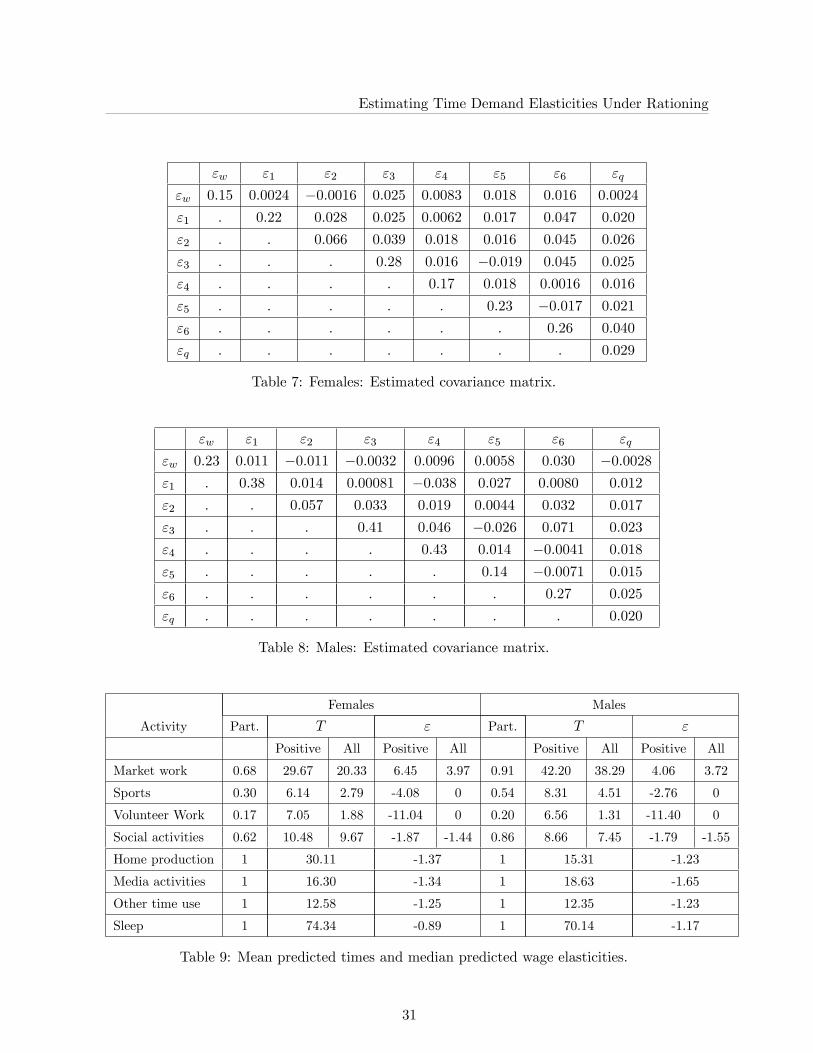
Tables 7 and 8 give the estimated covariance matrices for males and females. Examining
these tables shows females�unobserved preference for time in volunteer work is negative corre-
lated with the error in their wage equation. For males, the unobserved preferences for time in
both volunteer work and social activities are negatively correlated with the error in their wage
equation. For both males and females all other correlations of unobserved preferences with
the error in the wage equation are positive. It is interesting to note that the correlation of
the unobserved preferences for time in social activities and media activities is negative for both
males and females. This means individuals who have a high unobserved taste for time in media
activities are centris paribus likely to have a relatively low preference for time in social activities,
and vice versa. A similar interpretation can be given to the other correlations in these tables.
The parameters relating to demographic variables are most readily interpreted in terms of the
e¤ect they have of the wage elasticities and time allocations, see below.
The demand functions given by equations (14)-(16) and the wage elasticities given by equa-
tions (50) and (51) depend on both the observed individual speci�c heterogeneity, Zij , and the
20

Estimating Time Demand Elasticities Under Rationing
unobserved heterogeneity, "i. Since "i is unobserved the estimated elasticities and demand func-
tions are evaluated by simulation. To access the �t of the model and obtain wage elasticities for
the individuals in the sample the observed Zij and non labour market income for each individual
are used and 100 values of "i are drawn for each individual. Table 9 presents the results for this
simulation. The columns headed T give the mean predicted time in hours per week allocated to
each activity, and the columns headed " give the median wage elasticity of time in each activity.
<Table 9 about here>
Table 9 shows the model predicts women allocate more time than men to social activities,
home production and sleep, whereas men spend longer than women in market work, sports and
media activities. The mean predicted time allocated to volunteer work and other time use
is similar for men and women. This is entirely consistent with the observed time allocations
summarised in Table 1. The mean predicted time spent in market work is 20.33 hours per week
for women and 38.29 hours per week for men. This �gures compare favorably with the observed
hours of market work of 21.04 for women and 38.41 for men. The mean predicted times spent
in non market activities for men and women also mirror the observed time allocations.
<Figures 1 and 2 about here>
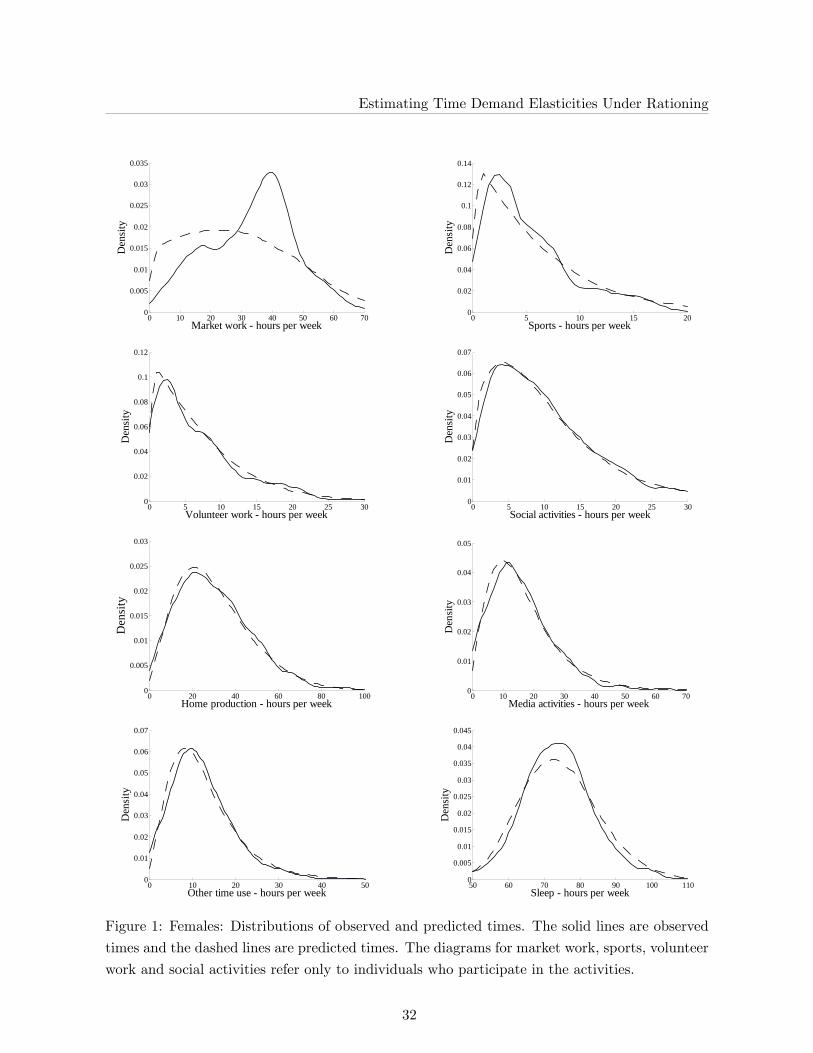
It is also insightful to look at the distributions of predicted times and compare these to the
distributions of observed times. These distributions are illustrated in Figure 1, for females, and
Figure 2, for males. For most non market activities the distributions of predicted and observed
times show a close resemblance. An exception occurs in the case of the time allocated to home
production by males. The distribution of predicted hours has a higher mode and is more skewed
to the right than the distribution of observed hours. Turning to market work, the distributions
of predicted and observed hours are decidedly di¤erent. For women, the distribution of observed
hours of market work has a small peak at around 20 hours per week, corresponding to part time
employment, and a larger peak at 40 hours per week, corresponding to full time employment.
However, the distribution of predicted hours of market work is much �atter and is unimodal.
For men, the distribution of observed hours is concentrated at 40 hours per week, however the
21

Estimating Time Demand Elasticities Under Rationing
distribution of predicted hours is again much �atter. These di¤erences are suggestive of there
being additional constraints on the time allocated to market work. These constraints may take
the form of individuals being unable to freely choose their hours of work, and instead facing a
choice between a �nite set of alternatives characterised by di¤erent hours of market work (for
an example in the context of the standard labour supply model see van Soest, 1995).
The model gives reasonable predictions of the proportions of non participants for market
work, sports, volunteer work and social activities, although these appear to be somewhat more
accurate for males than for females. A by product of predicting high proportions of non
participants in market work and non market activities is higher wage elasticities then those
commonly found in the labour supply literature. The results suggest a wage elasticity of
labour supply of 3.97% for females and 3.72% for males. For working individuals the median
wage elasticity of labour supply is 6.45% for females and 4.06% for males. As noted above,
this di¤erence is consistent with the functional form of the linear expenditure system and the
treatment of the zero observation. Ideally, one would specify a less restrictive functional form,
where the probability of non participation is not closely tied to the wage elasticity. This could
be achieved by using a functional form which does not restrict all non market activities to be
substitutes for market work. However, with more �exible functional forms ensuring coherency of
the demand system becomes more di¢ cult (see Diewert and Wales, 1987 and Pitt and Millimet,
2001). An alternative method of breaking the link between participation and the wage elasticity
would be to incorporate �xed costs of supplying time to activities, as suggested, in the context
of labour supply, by Cogan (1981). This would allow the model to predict non participation
without implying a large wage e¤ect. For labour supply, �xed costs might take the form of
transport or childcare costs. However, the presence of �xed costs of allocating time to non
market activities is less clear.
<Tables 10-12 about here>
Tables 10-12 detail the e¤ects of demographic variables on the probability of participation,
the wage elasticities and the allocation of time to market work and non market activities. The
results are based on a simulation of 1000 individuals and refer to individuals aged 30 with no
22

Estimating Time Demand Elasticities Under Rationing
children, a low level of education and a non labour market income of £ 20 per week. The e¤ect
of age is similar for males and females. A one year increase in an individual�s age increases
the time they spend in market work by an average of 0.53 hours per week for females and 0.63
hours per week for males. The probability an individual works in the market in also increasing
the individual�s age, whereas the wage elasticity of labour supply is decreasing in age. The
time spent in sports, social activities, other time use and sleep is decreasing in age for males
and females, whereas the time spent in social activities and home production is increasing in
age. The time spent in media activities is increasing in age for females and decreasing in age
for males. While some of these e¤ects appear large, it should be noted that age appears in
the wage equation and the demand functions in a quadratic form so the marginal e¤ect of age
depends on where the e¤ect is evaluated. For example, given the estimated parameter values,
the e¤ect of age on labour supply much smaller for individuals aged 50 than for individuals aged
30.
Table 11 shows the e¤ect of increasing education from a low level to a high level. For
females, education appears to mainly a¤ect the time allocated to market work, sports and
media activities. Females with a high level of education spend 1.84 hours per week longer in
market work than otherwise identical individuals with a low level of education. They also spend
1.48 hours per week longer in sports activities and 3.35 hours per week less in media activities.
In contrast, males with a high level of education spend 1.95 hours per week less in market work
than males with a low level of education. When education increases from a low level to a high
level, the time males spend in media activities and sleep decreases by 2.20 and 1.02 hours per
week respectively, and the time spent in sports and other time use increases by 2.64 and 2.44
hours per week respectively. Females with a high level of education are more likely to participate
in market work and social activities whereas males with a high level of education are less likely
to participate in these activities. For both males and females, a high level of education increases
the probability of participation in sports activities and decreases the probability of participation
in volunteer work.
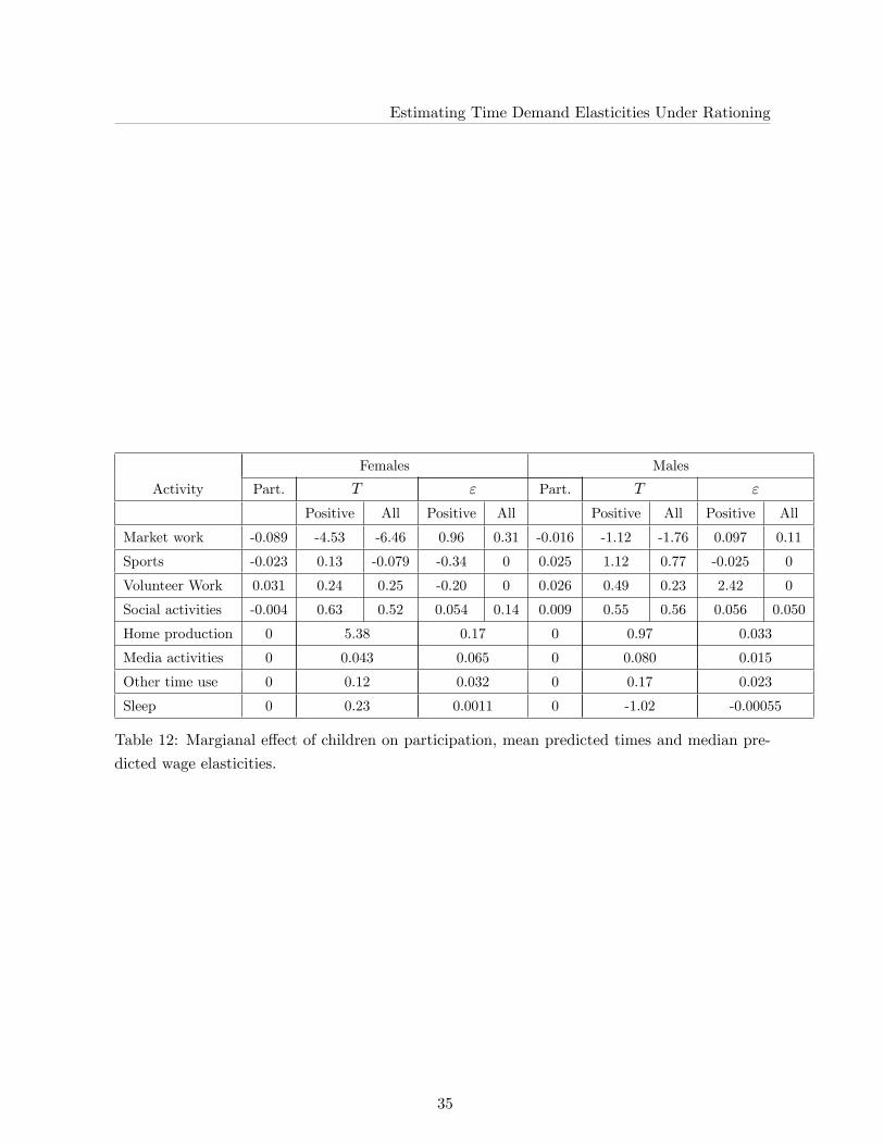
Finally, Table 12 shows the e¤ect of increasing the number of children present in the house-
hold from zero to one. For females, the greatest e¤ect of an increase in the number of children
23

Estimating Time Demand Elasticities Under Rationing
is on the time allocated to market work and home production. The presence of a child in the
household decreases the time spent in market work by 6.46 hour per week and increases the time
spent in home production by 5.38 hours per week. For males, the presence of a child reduces the
time spent in market work by 1.76 hours per week and decreases the time spent sleeping by 1.02
hours per week. The time spent in home production increases by 0.97 hours per week. Thus,
the presence of a child in the household appears to have a greater e¤ect on the time allocations
of women than of men.
6 Conclusion
A multivariate time allocation model with corner solutions in the time allocated to non market
activities and market work has been estimated, assuming Stone Geary preferences, which pro-
duces a linear expenditure system for the demand functions. Unobserved heterogeneity takes
the form of random preference variation and unobserved wage variation. The computation
problems posed by the high dimensional integrals in the likelihood have been circumvented by
using the GHK simulator.
The model gives reasonable predictions of the proportions individuals who do not participate
in market work and non market activities, and of the time allocated to market work and non
market activities. However, the estimated wage elasticity of labour supply is higher than
that typically found in the labour supply literature. This discrepancy has been attributed to
the functional form employed here, together with the high proportion of individuals who are
observed to be at a corner solution with respect to the time allocated to market work or non
market activities.
An interesting extension of this work would be to attempt to implement the multivariate
time allocation model using a more �exible functional form, where it would be possible to
accommodate individuals at corner solutions without constraining the wage elasticity to be high.
Another extension would be to attempt to incorporate additional constraints on the allocation
of time to market work and investigate whether this produces a distribution of predicted hours
of market work that more closely resembles the distribution of observed hours of market work.
24

Estimating Time Demand Elasticities Under Rationing
References
Börsh-Saupan, A. and V. Hajivassiliou (1993), Smooth unbiased multivariate probability sim-
ulators for maximum likelihood estimation of limited dependent variable models, Journal of
Econometrics, 58(3): 347-68.
Becker, G. (1965), A theory of the allocation of time, The Economic Journal, 75(299): 493-517.
Blundell, R. and T. MaCurdy (1999), Labour supply, in O. Ashenfelter and D. Card (eds.),
Handbook of Labor Economics, Vol 3a, Amsterdam: North Holland.
Cogan, J. (1981), Fixed costs and labor supply, Econometrica, 49(4): 945-963.
Diewert, W. and T. Wales (1987), Flexible functional forms and global curvature conditions,
Econometrica, 55(1): 43-68.
Gourieroux, C., J. La¤ont and A. Monfort (1980), Coherency conditions in simultaneous linear
equation models with endogenous switching regimes, Econometrica, 48(3): 675-696.
Hajivassiliou, V. and D. McFadden (1990), The method of simulated scores for the estimation of
LDV-models with an application to external debt crises; Cowles Foundation Discussion Paper,
Number 967; Yale University.
Hicks, J. (1936), Value and capital, Oxford, Oxford University Press.
Ipsos-RSL and O¢ ce for National Statistics, (2003), United Kingdom Time Use Survey, 2000,
3rd Edition, Colchester, Essex: UK Data Archive.
Juster, F. and F. Sta¤ord (1991), The allocation of time - Empirical �ndings, behavioral models,
and problems of measurement, Journal of Economic Literature 29(2): 471-522.
Keane, M. (1994), A computationally practical simulation estimator for panel data, Economet-
rica 62(1): 95-116.
Kiker, B. and M. Mendes de Oliveira (1992), Optimal allocation of time and estimation of
market wage functions, The Journal of Human Resources, 27(3): 445-471.
25

Estimating Time Demand Elasticities Under Rationing
Killingsworth, M. and J. Heckman (1986), Female labor Ssupply: a Survey, in Ashenfelter, O.
and P. Layard (eds.), Handbook of Labor Economics, Vol.1, Amsterdam: North Holland.
Kooreman, P. and A. Kapteyn (1987), A disaggregated analysis of the allocation of time within
the household, The Journal of Political Economy, 95(2): 223-249.
Lee, Lung-Fei. and M. Pitt (1986), Microeconometric demand system with binding nonnega-
tivity constraints: The dual approach, Econometrica, 54(5): 1237-1242.
Mroz, T. (1987), The sensitivity of an empirical model of married women�s hours of work to
economic and statistical assumptions, Econometrica, 55(4): 765-799.
Neary, J. P. and K. Roberts (1980), The theory of household behavior under rationing, European
Economic Review, 13(1):25-42.
Pollak, R. and M. Wachter (1975), The relevance of the household production function and its
implications for the allocation of time, The Journal of Political Economy, 83(2): 255-278.
Ransom, M. (1987), A comment on consumer demand systems with binding non negativity
constraints, Journal of Econometrics, 34(3): 355:359.
Stern, S. (1992), A method for smoothing simulated moments of discrete probabilities in multino-
mial probit models, Econometrica, 60(4): 943-952.
Stone, J. (1954), Linear expenditure systems and demand analysis: an application to the pattern
of British demand, Economic Journal, 64(255): 511-527.
Tobin, J. (1958), Estimation of relationships for limited dependent variables, Econometrica,
26(1): 24-36.
van Soest, A. (1995), Structural models of family labor supply: A discrete choice approach, The
Journal of Human Resources, 30(1): 63-88.
van Soest, A., A. Kapteyn and P. Kooreman (1993), Coherency and regularity of demand systems
with equality and inequality constraints, Journal of Econometrics, 57(1): 161-188.
26
Estimating Time Demand Elasticities Under Rationing
Wales, T. and A. Woodland (1980), Sample selectivity and the estimation of labor supply func-
tions, International Economic Review, 21(2): 437-68.
� � � � (1983), Estimation of consumer demand systems with binding non-negativity con-
straints, Journal of Econometrics, 21(3): 263-285.
27

Estimating Time Demand Elasticities Under Rationing
Activity Females Males
1832 observations 1433 observations
Part Positive All Part Positive All
Market work 0:63 33:40 21:04 0:86 45:08 38:41
Sports 0:45 6:12 2:75 0:54 8:45 4:55
Volunteer Work 0:27 7:03 1:89 0:11 6:02 1:24
Social activities 0:91 10:38 9:49 0:86 8:67 7:49
Home production 0:99 30:24 30:01 0:97 15:64 15:12
Media activities 0:97 16:55 16:09 0:98 19:00 18:68
Other time use 0:99 12:70 12:58 0:99 12:49 12:43
Sleep 1 74:15 74:15 1 70:09 70:09
Table 1: Summary of Time Use data: Hours per equivalent week.
Category Females Males Category Females Males
W;Sp; V; Sc 118 112 W;Sp; V; Sc 81 20
W;Sp; V; Sc 158 98 W;Sp; V ; Sc 216 84
W;Sp; V ; Sc 336 438 W;Sp; V; Sc 4 1
W;Sp; V; Sc 6 5 W;Sp; V ; Sc 65 84
W;Sp; V; Sc 112 45 W;Sp; V ; Sc 206 47
W;Sp; V ; Sc 448 394 W;Sp; V; Sc 4 0
W;Sp; V; Sc 8 13 W;Sp; V ; Sc 15 10
W;Sp; V ; Sc 15 77 W;Sp; V ; Sc 40 5
Table 2: Number of individuals falling into each combination of binding and non binding non
negativity constraints: W, Sp, V and Sc denote Market work, Sports, Volunteer work and Social
activities respectively. An underscore denotes a zero observation for the corresponding activitiy.
Females Males
Mean s.d Mean s.d
Age 39:84 11:01 40:50 11:62
Education 0:28 0:45 0:29 0:46
Children 1:22 1:25 1:05 1:16
Wage 6:64 5:05 8:43 5:54
Table 3: Summary of demograpgic and wage data.
28

Estimating Time Demand Elasticities Under Rationing
Females Males
1 �13:25(0:58)
�10:13(0:65)
2 �53:04(1:38)
�52:19(1:87)
3 �7:22(0:42)
�5:28(0:36)
4 �13:57(0:77)
�3:62(0:39)
5 �7:71(0:48)
�12:96(0:63)
6 �4:78(0:40)
�3:22(0:37)
7 4:50(0:028)
�15:07(0:83)
q �38327:45(886:50)
�43162:57(909:48)
Table 4: Estimates of j for j=1,...,7 and q for females and males. Standard errors in paren-
thesis. 1,..., 7 correspond to sports, volunteer work, social activities, home production, media
activities, other time use and sleep respectively.
Females Males
Intercept 1:16(0:088)
1:34(0:15)
Age 0:021(0:0048)
0:024(0:0069)
Age2 �0:00022(0:000066)
�0:00023(0:000083)
Education 0:44(0:025)
0:33(0:029)
Table 5: Estimated of parameters of the wage equation for females and males.
29

Estimating Time Demand Elasticities Under Rationing
Females Males Females Males
�1 �5
Intercept �1:94(0:18)
�2:04(0:21)
Intercept �1:34(0:12)
�1:14(0:10)
Age 0:0085(0:0097)
�0:0031(0:011)
Age 0:0083(0:0064)
0:0024(0:0054)
Age2 �0:000072(0:00011)
0:000010(0:00013)
Age2 �0:000052(0:000076)
0:000013(0:0063)
Education 0:13(0:027)
0:22(0:039)
Education �0:13(0:026)
�0:079(0:022)
Number of children �0:019(0:011)
0:033(0:017)
Number of children �0:019(0:020)
�0:0044(0:0093)
�2 �6
Intercept �0:78(0:086)
�0:98(0:076)
Intercept �1:53(0:16)
�1:83(0:17)
Age 0:014(0:0040)
0:011(0:0041)
Age 0:0046(0:0085)
�0:0010(0:0093)
Age2 �0:011(0:000047)
�0:000091(0:000048)
Age2 �0:00011(0:000097)
�0:00001(0:011)
Education 0:000001(0:016)
0:000006(0:018)
Education 0:066(0:026)
0:15(0:031)
Number of children 0:013(0:0063)
0:019(0:0076)
Number of children 0:019(0:010)
0:028(0:013)
�3 �q
Intercept �0:94(0:16)
�1:55(0:18)
Intercept 4:73(0:054)
4:55(0:15)
Age �0:033(0:0077)
�0:030(0:0090)
Age �0:0004(0:0043)
�0:0064(0:0081)
Age2 0:00041(0:000092)
0:00038(0:00011)
Age2 �0:000027(0:0061)
0:000030(0:000057)
Education 0:023(0:028)
�0:0018(0:038)
Education �0:42(0:026)
�0:32(0:030)
Number of children 0:019(0:011)
0:0013(0:016)
Number of children �0:012(0:0038)
0:0052(0:0035)
�4
Intercept �1:02(0:11)
�2:4616(0:23)
Age 0:0079(0:0055)
0:0148(0:013)
Age2 0:000004(0:000066)
0:000009(0:014)
Education �0:019(0:022)
0:0135(0:039)
Number of children 0:13(0:0090)
0:1165(0:017)
Table 6: Estimates of �j for j=1,...,6 and �q for males and females. Standard errors in paren-
thesis. �1,...,�6 correspond to sports, volunteer work, social activities, home production, media
activities and other time use respectively.
30
Estimating Time Demand Elasticities Under Rationing
"w "1 "2 "3 "4 "5 "6 "q
"w 0:15 0:0024 �0:0016 0:025 0:0083 0:018 0:016 0:0024
"1 : 0:22 0:028 0:025 0:0062 0:017 0:047 0:020
"2 : : 0:066 0:039 0:018 0:016 0:045 0:026
"3 : : : 0:28 0:016 �0:019 0:045 0:025
"4 : : : : 0:17 0:018 0:0016 0:016
"5 : : : : : 0:23 �0:017 0:021
"6 : : : : : : 0:26 0:040
"q : : : : : : : 0:029
Table 7: Females: Estimated covariance matrix.
"w "1 "2 "3 "4 "5 "6 "q
"w 0:23 0:011 �0:011 �0:0032 0:0096 0:0058 0:030 �0:0028"1 : 0:38 0:014 0:00081 �0:038 0:027 0:0080 0:012
"2 : : 0:057 0:033 0:019 0:0044 0:032 0:017
"3 : : : 0:41 0:046 �0:026 0:071 0:023
"4 : : : : 0:43 0:014 �0:0041 0:018
"5 : : : : : 0:14 �0:0071 0:015
"6 : : : : : : 0:27 0:025
"q : : : : : : : 0:020
Table 8: Males: Estimated covariance matrix.
Females Males
Activity Part. T " Part. T "
Positive All Positive All Positive All Positive All
Market work 0.68 29.67 20.33 6.45 3.97 0.91 42.20 38.29 4.06 3.72
Sports 0.30 6.14 2.79 -4.08 0 0.54 8.31 4.51 -2.76 0
Volunteer Work 0.17 7.05 1.88 -11.04 0 0.20 6.56 1.31 -11.40 0
Social activities 0.62 10.48 9.67 -1.87 -1.44 0.86 8.66 7.45 -1.79 -1.55
Home production 1 30.11 -1.37 1 15.31 -1.23
Media activities 1 16.30 -1.34 1 18.63 -1.65
Other time use 1 12.58 -1.25 1 12.35 -1.23
Sleep 1 74.34 -0.89 1 70.14 -1.17
Table 9: Mean predicted times and median predicted wage elasticities.
31
Estimating Time Demand Elasticities Under Rationing
0 10 20 30 40 50 60 700
0.005
0.01
0.015
0.02
0.025
0.03
0.035
Market work - hours per week
Den
sity
0 5 10 15 200
0.02
0.04
0.06
0.08
0.1
0.12
0.14
Sports - hours per week
Den
sity
0 5 10 15 20 25 300
0.02
0.04
0.06
0.08
0.1
0.12
Volunteer work - hours per week
Den
sity
0 5 10 15 20 25 300
0.01
0.02
0.03
0.04
0.05
0.06
0.07
Social activities - hours per week
Den
sity
0 20 40 60 80 1000
0.005
0.01
0.015
0.02
0.025
0.03
Home production - hours per week
Den
sity
0 10 20 30 40 50 60 700
0.01
0.02
0.03
0.04
0.05
Media activities - hours per week
Den
sity
0 10 20 30 40 500
0.01
0.02
0.03
0.04
0.05
0.06
0.07
Other time use - hours per week
Den
sity
50 60 70 80 90 100 1100
0.005
0.01
0.015
0.02
0.025
0.03
0.035
0.04
0.045
Sleep - hours per week
Den
sity
Figure 1: Females: Distributions of observed and predicted times. The solid lines are observed
times and the dashed lines are predicted times. The diagrams for market work, sports, volunteer
work and social activities refer only to individuals who participate in the activities.
32

Estimating Time Demand Elasticities Under Rationing
0 10 20 30 40 50 60 700
0.005
0.01
0.015
0.02
0.025
0.03
0.035
0.04
Market work - hours per week
Den
sity
0 5 10 15 200
0.02
0.04
0.06
0.08
0.1
0.12
Sports - hours per week
Den
sity
0 5 10 15 200
0.02
0.04
0.06
0.08
0.1
0.12
Volunteer work - hours per week
Den
sity
0 5 10 15 20 25 300
0.01
0.02
0.03
0.04
0.05
0.06
0.07
0.08
0.09
Social activities - hours per week
Den
sity
0 20 40 60 80 1000
0.005
0.01
0.015
0.02
0.025
0.03
0.035
0.04
0.045
Home production - hours per week
Den
sity
0 10 20 30 40 50 60 700
0.01
0.02
0.03
0.04
0.05
Media activities - hours per week
Den
sity
0 10 20 30 40 500
0.01
0.02
0.03
0.04
0.05
0.06
0.07
Other time use - hours per week
Den
sity
50 60 70 80 90 100 1100
0.005
0.01
0.015
0.02
0.025
0.03
0.035
0.04
0.045
Sleep - hours per week
Den
sity
Figure 2: Males: Distributions of observed and predicted times. The solid lines are observed
times and the dashed lines are predicted times. The diagrams for market work, sports, volunteer
work and social activities refer only to individuals who participate in the activities.
33

Estimating Time Demand Elasticities Under Rationing
Females Males
Activity Part. T " Part. T "
Positive All Positive All Positive All Positive All
Market work 0.007 0.35 0.53 -0.061 -0.0048 0.001 0.61 0.63 -0.066 -0.061
Sports 0 -0.013 -0.0052 -0.0194 0 -0.002 -0.098 -0.063 -0.0072 0
Volunteer Work 0.001 0.11 0.026 0.099 0 0.001 0.011 0.0076 0.037 0
Social activities -0.003 -0.20 -0.22 -0.015 -0.017 -0.003 -0.14 -0.14 -0.010 -0.010
Home production 0 0.12 -0.0011 0 0.15 0.0056
Media activities 0 0.0071 -0.0032 0 -0.054 -0.0014
Other time use 0 -0.12 -0.0069 0 -0.10 -0.0022
Sleep 0 -0.34 0.00032 0 -0.43 -0.0009
Table 10: Margianal e¤ect of age on participation, mean predicted times and median predicted
wage elasticities.
Females Males
Activity Part. T " Part. T "
Positive All Positive All Positive All Positive All
Market work 0.017 1.48 1.84 -0.42 -0.063 -0.016 -1.33 -1.95 0.14 0.13
Sports 0.13 1.33 1.48 0.58 0 0.14 2.55 2.64 0.41 -1.48
Volunteer Work -0.013 -0.72 -0.21 -1.46 0 -0.004 -0.35 -0.067 -0.76 0
Social activities 0.003 0.14 0.16 0.014 -0.0068 -0.003 -0.056 -0.075 0.044 0.055
Home production 0 -0.39 0.010 0 0.25 0.016
Media activities 0 -3.35 -0.063 0 -2.20 -0.048
Other time use 0 0.47 0.014 0 2.44 0.068
Sleep 0 -0.0059 0.013 0 -1.02 0.012
Table 11: Margianal e¤ect of education on participation, mean predicted times and median
predicted wage elasticities.
34
Estimating Time Demand Elasticities Under Rationing
Females Males
Activity Part. T " Part. T "
Positive All Positive All Positive All Positive All
Market work -0.089 -4.53 -6.46 0.96 0.31 -0.016 -1.12 -1.76 0.097 0.11
Sports -0.023 0.13 -0.079 -0.34 0 0.025 1.12 0.77 -0.025 0
Volunteer Work 0.031 0.24 0.25 -0.20 0 0.026 0.49 0.23 2.42 0
Social activities -0.004 0.63 0.52 0.054 0.14 0.009 0.55 0.56 0.056 0.050
Home production 0 5.38 0.17 0 0.97 0.033
Media activities 0 0.043 0.065 0 0.080 0.015
Other time use 0 0.12 0.032 0 0.17 0.023
Sleep 0 0.23 0.0011 0 -1.02 -0.00055
Table 12: Margianal e¤ect of children on participation, mean predicted times and median pre-
dicted wage elasticities.
35
Related Documents


