Electronic copy available at: http://ssrn.com/abstract=1054721 Estimating the Wishart Affine Stochastic Correlation Model using the Empirical Characteristic Function * Jos´ e Da Fonseca † Martino Grasselli ‡ Florian Ielpo § First draft: November 27, 2007 This draft: November 10, 2008 Abstract This paper provides the first estimation strategy for the Wishart Affine Stochastic Correlation (WASC) model. We provide elements to show that the utilization of em- pirical characteristic function-based estimates is advisable: this function is exponential affine in the WASC case. We use a GMM estimation strategy with a continuum of moment conditions based on the characteristic function. We present the estimation results obtained using a dataset of equity indexes. The WASC model captures most of the known stylized facts associated with financial markets, including the leverage and asymmetric correlation effects. Keywords: Wishart Process, Empirical Characteristic Function, Stochastic Correlation, Generalized Method of Moments. * Acknowledgements: We are particularly indebted to Marine Carrasco for remarkable insights and helpful comments. We are also grateful to Christian Gourieroux, Fulvio Pegoraro, Fran¸cois-Xavier Vialard and the CREST seminar participants for useful remarks. We are thankful to the seminar participants of the 14th International Conference on Computing in Economics and Finance, Paris, France (2008), the 11th conference of the Swiss Society for Financial Market Research, Z¨ urich (2008), Mathematical and Statistical Methods for Insurance and Finance, Venice, Italy (2008), the 2nd International Workshop on Computa- tional and Financial Econometrics, Neuchˆ atel, Switzerland (2008), the First PhD Quantitative Finance Day, Swiss Banking Institute, Z¨ urich (2008), Inference and tests in Econometrics, in the honor of Russel Davidson, Marseille, France (2008), the Inaugural conference of the Society for Financial Econometrics (SoFie), New York, USA (2008), the 28th International Symposium on Forecasting, Nice, France (2008), the ESEM annual meeting, Milano, Italy (2008), the Oxford-Man Institute of Quantitative Finance Vast Data Conference, Oxford, UK (2008), the Courant Institute Mathematical Finance seminar, New York, USA (2008) and the Bloomberg Seminar, New York, USA (2008) for their comments and remarks. Any errors remain ours. † Ecole Sup´ erieure d’Ing´ enieurs L´ eonard de Vinci, D´ epartement Math´ ematiques et Ing´ enierie Financi` ere, 92916 Paris La D´ efense, France. Email: jose.da [email protected] and Zeliade Systems, 56, Rue Jean- Jacques Rousseau, 75001 Paris. ‡ Universit` a degli Studi di Padova , Dipartimento di Matematica Pura ed Applicata, Via Trieste 63, Padova, Italy. E-mail: [email protected] and ESILV. § Pictet & Cie, Route des Acacias 60, CH-1211 Gen` eve 73. E-mail: fl[email protected]. 1

Welcome message from author
This document is posted to help you gain knowledge. Please leave a comment to let me know what you think about it! Share it to your friends and learn new things together.
Transcript
Electronic copy available at: http://ssrn.com/abstract=1054721
Estimating the Wishart Affine Stochastic Correlation Model
using the Empirical Characteristic Function∗
Jose Da Fonseca† Martino Grasselli‡ Florian Ielpo§
First draft: November 27, 2007
This draft: November 10, 2008
Abstract
This paper provides the first estimation strategy for the Wishart Affine StochasticCorrelation (WASC) model. We provide elements to show that the utilization of em-pirical characteristic function-based estimates is advisable: this function is exponentialaffine in the WASC case. We use a GMM estimation strategy with a continuum ofmoment conditions based on the characteristic function. We present the estimationresults obtained using a dataset of equity indexes. The WASC model captures mostof the known stylized facts associated with financial markets, including the leverageand asymmetric correlation effects.
Keywords: Wishart Process, Empirical Characteristic Function, Stochastic Correlation,
Generalized Method of Moments.
∗ Acknowledgements: We are particularly indebted to Marine Carrasco for remarkable insights andhelpful comments. We are also grateful to Christian Gourieroux, Fulvio Pegoraro, Francois-Xavier Vialardand the CREST seminar participants for useful remarks. We are thankful to the seminar participants ofthe 14th International Conference on Computing in Economics and Finance, Paris, France (2008), the 11thconference of the Swiss Society for Financial Market Research, Zurich (2008), Mathematical and StatisticalMethods for Insurance and Finance, Venice, Italy (2008), the 2nd International Workshop on Computa-tional and Financial Econometrics, Neuchatel, Switzerland (2008), the First PhD Quantitative FinanceDay, Swiss Banking Institute, Zurich (2008), Inference and tests in Econometrics, in the honor of RusselDavidson, Marseille, France (2008), the Inaugural conference of the Society for Financial Econometrics(SoFie), New York, USA (2008), the 28th International Symposium on Forecasting, Nice, France (2008),the ESEM annual meeting, Milano, Italy (2008), the Oxford-Man Institute of Quantitative Finance VastData Conference, Oxford, UK (2008), the Courant Institute Mathematical Finance seminar, New York,USA (2008) and the Bloomberg Seminar, New York, USA (2008) for their comments and remarks. Anyerrors remain ours.†Ecole Superieure d’Ingenieurs Leonard de Vinci, Departement Mathematiques et Ingenierie Financiere,
92916 Paris La Defense, France. Email: jose.da [email protected] and Zeliade Systems, 56, Rue Jean-Jacques Rousseau, 75001 Paris.‡Universita degli Studi di Padova , Dipartimento di Matematica Pura ed Applicata, Via Trieste 63,
Padova, Italy. E-mail: [email protected] and ESILV.§Pictet & Cie, Route des Acacias 60, CH-1211 Geneve 73. E-mail: [email protected].
1
Electronic copy available at: http://ssrn.com/abstract=1054721
1 Introduction
The estimation of continuous time processes under the physical measure attracted a lot
of attention over the few past years, and several estimation strategies have been proposed
in the literature. When the transition density is known in closed form, it is possible to
perform a maximum likelihood estimation of the diffusion parameters, as presented e.g.
in Lo (1988). However, the number of models for which the transition density is known
in a closed form expression is somewhat limited. Moreover, the existence of unobserved
factors such as the volatility process in the Heston (1993) model makes it difficult – if not
impossible – to estimate such models using a conditional maximum likelihood approach.
A possible solution consists in discretizing and simulating the unobservable process: for
example, Duffie and Singleton (1993) used the Simulated Methods of Moments to esti-
mate financial Markov processes (methods of this kind are reviewed in Gourieroux and
Monfort, 1996). However, as pointed out in Chacko and Viceira (2003), even though these
methods are straightforward to apply, it is difficult to measure the numerical errors due
to the discretization. What is more, the computational burden of this class of methods
precludes its use for multivariate processes.
For the special class of affine models, another estimation strategy can be used. The
affine models present tractable exponentially affine characteristic functions that can in
turn be used to estimate the parameters under the historical measure. Singleton (2001)
and Singleton (2006) present a list of possible estimation strategies that can be applied
to recover these parameters from financial time series, using the characteristic function of
the process. Methodologies of this kind have been applied to one-dimensional processes,
like the Cox-Ingersoll-Ross process (e.g. Zhou, 2000), the Heston process and a mixture
of stochastic volatility and jump processes (e.g. Jiang and Knight, 2002, Rockinger and
Semenova, 2005 and Chacko and Viceira, 2003) and affine jump diffusion models (e.g.
Yu, 2004), yielding interesting results. Still, it involves additional difficulties. First, as
remarked in Jiang and Knight (2002) and Rockinger and Semenova (2005), numerically
integrating the characteristic function of a vector of the state variable is computationally
intensive. In our multivariate case the state variable is already a vector: for this type of
methodology, the integral discretization is likely to lead to numerical errors. Second, with
the Spectral GMM method presented in Chacko and Viceira (2003), the use of a more
limited number of points of the characteristic function settles the numerical problem, but
leads to a decrease in estimates efficiency. Carrasco and Florens (2000) and Carrasco
2
et al. (2007) present a method that uses a continuum of moment conditions built from the
characteristic function. With this method, the estimates obtained reach the efficiency of
the maximum likelihood method, thanks to the instrument used in this strategy. These
features make this methodology particularly well-suited for the estimation of affine multi-
variate continuous time processes.
Here, we propose to use a Spectral Generalized Method of Moments estimation strategy to
estimate the Wishart Affine Stochastic Correlation model, an affine multivariate stochas-
tic volatility and correlation model introduced in Da Fonseca et al. (2007). Based on the
previous models of Gourieroux and Sufana (2004), this affine model can be regarded as a
multivariate version of the Heston (1993) model: in fact, the volatility matrix is assumed
to evolve according to the Wishart dynamics (mathematically developed by Bru, 1991),
the matrix analogue of the mean reverting square root process. In addition to the Heston
model, it allows for a stochastic conditional correlation, which makes it very promising
process for financial applications. Buraschi et al. (2006) independently proposed a related
model corresponding to a constrained correlation version of the WASC model.
Multivariate stochastic volatility models have recently attracted a great deal of attention.
Bauwens et al. (2006) and Asai et al. (2006) present a survey of the existing models, along
with estimation methodologies. When compared to the previously mentioned processes,
several important differences must be underlined. (1) The volatility being a latent factor,
the observable state variable (the asset log returns) is not Markov anymore and the ML
efficiency cannot be reach. (2) What is more, as we discuss it in the paper, since the
process involves latent volatilities and correlations, the instrument must be set to be equal
to one for the usual GMM methodology to be used. This precludes the use of the Double
Index instruments procedure presented in Carrasco et al. (2007). (3) Since correlations
are also stochastic, there are more latent variables than in the stochastic volatility models,
making simulation-based methods useless. (4) Finally, the dimensionality of the problem
makes the characteristic function difficult to invert.
In view of these difficulties, we propose to estimate the WASC model using its charac-
teristic function, following an approach that is closed to the ones presented in Chacko
and Viceira (2003) and Carrasco et al. (2007). We present a Monte Carlo investigation of
the estimates’ behavior in a small sample and we discuss the empirical results obtained
using a real dataset composed of the prices of the SP500, FTSE, DAX and CAC 40. Our
3
results unfold as follow. (1) The estimated WASC parameters are comparable to what
is obtained in the univariate empirical literature. (2) Thanks to its ability to describe
dynamic correlation, the WASC model can encompass most of the desired features of fi-
nancial markets: it reveals asymmetric correlation and leverage effects. (3) Our estimates
reject systematically the particular correlation structure chosen by Gourieroux and Sufana
(2004) and Buraschi et al. (2006), favoring the flexibility of the specification presented in
Da Fonseca et al. (2007).
The paper is organized as follows. First we present the WASC process, along with the
computation of its conditional characteristic function. In Section 3, we present the esti-
mation methodology used in this paper and briefly review the main theoretical results.
Finally, in Section 4, we present the estimation results obtained with both simulated and
real datasets and discuss their interpretation.
2 The model
In this section, we present the Wishart Affine Stochastic Correlation model introduced in
Da Fonseca et al. (2007): we detail the diffusion that drives this multidimensional process
and present the conditional characteristic function together with its derivatives.
2.1 The dynamics
The Wishart Affine Stochastic Correlation (WASC) model is a new continuous time process
that can be considered as a multivariate extension of the Heston (1993) model, with a more
accurate correlation structure. The framework of this model was introduced in Gourieroux
and Sufana (2004). It relies on the following assumption.
Assumption 2.1. The evolution of asset returns is conditionally Gaussian while the
stochastic variance-covariance matrix follows a Wishart process.
In formulas, we consider a n-dimensional risky asset St whose risk-neutral dynamics are
given by
dSt = diag[St](µdt+
√ΣtdZt
), (1)
where µ is the vector of returns and Zt ∈ Rn is a vector Brownian motion. Following
Gourieroux and Sufana (2004), we assume that the quadratic variation of the risky assets
4
is a matrix Σt which is assumed to satisfy the following dynamics:
dΣt =(
ΩΩ> +MΣt + ΣtM>)dt+
√ΣtdWtQ+Q> (dWt)
>√Σt, (2)
with Ω,M,Q ∈ Mn, Ω invertible, and Wt ∈ Mn a matrix Brownian motion (> denotes
transposition). In the present framework we assume that the above dynamics are inferred
from observed asset price time series, hence the stochastic differential equation is written
under the historical measure.
Equation (2) characterizes the Wishart process introduced by Bru (1991), and represents
the matrix analogue of the square root mean-reverting process. In order to ensure the
strict positivity and the typical mean-reverting feature of the volatility, the matrix M is
assumed to be negative semi-definite, while Ω satisfies
ΩΩ> = βQ>Q, β > n− 1, (3)
with the real parameter β > n− 1 (see Bru, 1991 p. 747).
In full analogy with the square-root process, the term ΩΩ> is related to the expected long-
term variance-covariance matrix Σ∞ through the solution to the following linear equation:
−ΩΩ> = MΣ∞ + Σ∞M>. (4)
Moreover, Q is the volatility of the volatility matrix, and its parameters will be crucial in
order to explain some stylized observed effects in equity markets.
Last but not least, Da Fonseca et al. (2007) proposed a very special yet tractable corre-
lation structure that is able to accommodate the leverage effects found in financial time
series and option prices. Since it is well known that it is possible to approximately repro-
duce observed negative skewness within the Heston (1993) model by allowing for negative
correlation between the noise driving returns and the noise driving variance, they proposed
the following assumption:
Assumption 2.2. The Brownian motions of the asset returns and those driving the co-
variance matrix are linearly correlated.
Da Fonseca et al. (2007) proved that Assumption 2.2. leads to the following relation:
dZt = dWtρ+√
1− ρ>ρdBt, (5)
5
with Zt = (dZ1, dZ2, . . . , dZn)>, B a vector of independent Brownian motions orthogonal
to W , as defined in equation (2), and ρ = (ρ1, ρ2, . . . , ρn)>.
With this specification, the model is able to generate negative skewness, given the possibly
negative correlation between the noise driving the log returns of the assets and the matrix-
sized noise perturbating the covariance matrix. This is easy to show in the special case of
two assets (n = 2), fow which the variance-covariance matrix is given by
Σt =
Σ11t Σ12
t
Σ12t Σ22
t
. (6)
The correlations between assets’ returns and their volatilities admit a closed form expres-
sion, highlighting the impact of the ρ parameters on its value and positivity:
corr(d logS1, dΣ11
)=ρ1Q11 + ρ2Q21√
Q211 +Q2
21
(7)
corr(d logS2, dΣ22
)=ρ1Q12 + ρ2Q22√
Q212 +Q2
22
, (8)
where we recall that√
Σ11 (resp.√
Σ22) represents the volatility of the first (resp. second)
asset. Therefore, the sign and magnitude of the skew effects are determined by both the
matrix Q and the vector ρ. When Q is diagonal, we obtain the following skews for asset
1 and 2:
corr(d logS1, dΣ11
)= ρ1 corr
(d logS2, dΣ22
)= ρ2, (9)
thus allowing a negative skewness for each asset whenever ρi < 0,∀i (see Gourieroux and
Jasiak (2001) on this point). This correlation structure is similar the one obtained in an
Heston model.
Other less general specifications close to the WASC model, actually nested within the
WASC correlation structure, have been proposed in the literature. First, Gourieroux and
Sufana (2004) imposed ρ = 0n ∈ Rn, a choice that leads to a zero correlation case (see
equations (5), (7) and (8)) by analogy with the well known properties of the Heston model.
With this specification, the log returns’ univariate distribution is symmetric.
Second, Buraschi et al. (2006) proposed to impose ρ = (1, 0)>. Their model is thus able
to display negative skewness for asset 1 (resp. asset 2), depending on the positivity of
Q11 (resp. Q12). This model is actually close to the WASC and is able to display similar
6
features. Their choice of ρ is less restrictive than it seems, in so far as this parameter
is only defined up to a rotation. Thus, their hypothesis is reduced to ||ρ|| = 1. With
these settings, the vector-sized noise in the returns is fully generated by the Brownian
motions of the covariances W . This hypothesis having no a priori justification, the WASC
model of Da Fonseca et al. (2007) eliminates it, assuming the more general correlation
structure compatible with an exponential affine characteristic function (see Proposition 1
in Da Fonseca et al. (2007) on this point).
2.2 The Characteristic functions
In the WASC model, the characteristic function of Σt and Yt = logSt is an exponential
affine function of the state variables. For the log returns, the characteristic function of
Yt+τ conditional on Yt and Σt is denoted:
ΦYt,Σt(τ, ω) = E[ei〈ω,Yt+τ 〉|Σt, Yt
], (10)
where E[.|Σt, Yt] denotes the conditional expected value with respect to the historical
measure, ω ∈ Rn, i2 = −1 and 〈., .〉 is the scalar product in Rn.
Proposition 2.1. (Da Fonseca et al., 2007) The characteristic function of the asset re-
turns in the WASC model is given by
ΦYt,Σt(τ, ω) = E[ei〈ω,Yt+τ 〉|Σt, Yt
](11)
= exp Tr [A(τ)Σt] + 〈iω, Yt〉+ c(τ) , (12)
where ω = (ω1, . . . , ωn)> ∈ Rn and the deterministic function A(t) ∈Mn is as follows:
A (τ) = A22 (τ)−1A21 (τ) , (13)
with
A11 (τ) A12 (τ)
A21 (τ) A22 (τ)
= exp τ
M +Q>ρiω> −2Q>Q
12
((iω)(iω)> −
∑nj=1 iωjejj
)−(M> + iωρ>Q
) .
(14)
7
The function c(τ) can be obtained by direct integration, thus giving:
c(τ) = −β2
Tr[log (A22(τ)) + τM> + τiω(ρ>Q)
]+ τTr
[µiω>
]. (15)
The characteristic function of the Wishart process is defined as:
ΦΣt(τ,∆) = E[eiTr[∆Σt+τ ]|Σt
], (16)
where ∆ ∈Mn.
Proposition 2.2. (Da Fonseca et al., 2007) Given a real symmetric matrix D, the con-
ditional characteristic function of the Wishart process Σt is given by:
ΦΣt(τ,∆) = E[eiTr[∆Σt+τ ]|Σt
]= exp Tr [B(τ)Σt] + C(τ) , (17)
where the deterministic complex-valued functions B(τ) ∈Mn(Cn), C(τ) ∈ C are given by
B (τ) = (i∆B12 (τ) +B22 (τ))−1 (i∆B11 (τ) +B21 (τ)) (18)
C(τ) = −β2
Tr[log(i∆B12(τ) +B22(τ)) + τM>
],
with B11 (τ) B12 (τ)
B21 (τ) B22 (τ)
= exp τ
M −2Q>Q
0 −M>
.
What is more, these characteristic functions can be derived with respect to β and the
elements of M , Q and ρ, using the results of Daleckii (1974), on the derivative of a matrix
function. We provide detailed calculations of these derivatives in the Appendix.
3 Spectral GMM in the WASC setting
In this section, we present the detailed estimation methodology used for the WASC model.
In this paper, we are in the special setting where the correlation and variance processes are
unobserved. In this case, the feasible estimation strategies are: (1) to filtrate covariances
8
out of return time series either (a) using DCC estimates, (b) a GARCH-like discretization
of the continuous time process or (c) a linearized Kalman filter; (2) to estimate the process
using the conditional characteristic function. We favor the second type of methodologies
since (1) DCC-based estimates of the ρ parameter are biased1 and (2) any type of dis-
cretization or linearization will lead to additional estimation errors. In the WASC case,
the characteristic function is known in a closed form expression, thus being a very suitable
tool for the estimation of vector-processes, especially when compared to simulation-based
estimators. For further discussion on the estimation strategies of Wishart-based models,
see Gourieroux (2006).
Recent articles presented estimation methodologies using the empirical characteristic func-
tion as an estimation tool, since this function has a tractable expression for many con-
tinuous time processes. In this section, we present how to estimate the WASC in this
framework, building on the approaches developed in Chacko and Viceira (2003) and Car-
rasco et al. (2007).
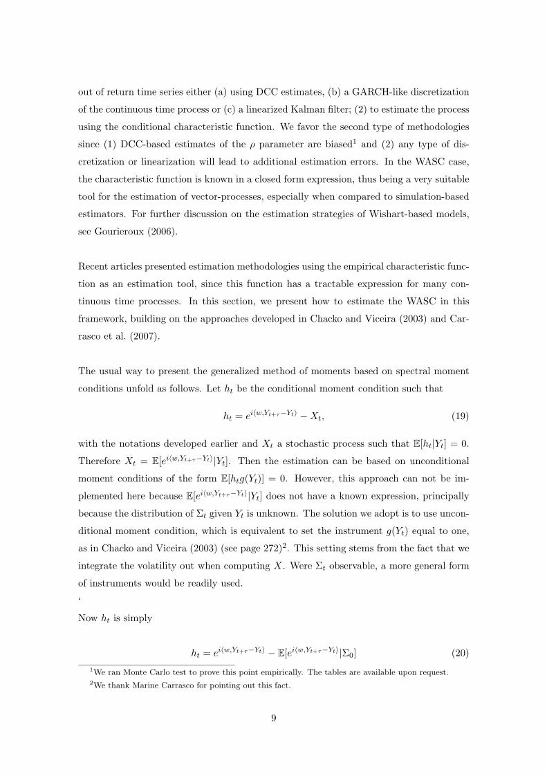
The usual way to present the generalized method of moments based on spectral moment
conditions unfold as follows. Let ht be the conditional moment condition such that
ht = ei〈w,Yt+τ−Yt〉 −Xt, (19)
with the notations developed earlier and Xt a stochastic process such that E[ht|Yt] = 0.
Therefore Xt = E[ei〈w,Yt+τ−Yt〉|Yt]. Then the estimation can be based on unconditional
moment conditions of the form E[htg(Yt)] = 0. However, this approach can not be im-
plemented here because E[ei〈w,Yt+τ−Yt〉|Yt] does not have a known expression, principally
because the distribution of Σt given Yt is unknown. The solution we adopt is to use uncon-
ditional moment condition, which is equivalent to set the instrument g(Yt) equal to one,
as in Chacko and Viceira (2003) (see page 272)2. This setting stems from the fact that we
integrate the volatility out when computing X. Were Σt observable, a more general form
of instruments would be readily used.
‘
Now ht is simply
ht = ei〈w,Yt+τ−Yt〉 − E[ei〈w,Yt+τ−Yt〉|Σ0] (20)1We ran Monte Carlo test to prove this point empirically. The tables are available upon request.2We thank Marine Carrasco for pointing out this fact.
9
where the initial value of Σ0 is treated as an unknown parameter to be estimated. We
have
E[ei〈w,Yt+τ−Yt〉|Σ0] = ec(τ)E[e〈A(τ),Σt〉|Σ0] = ec(τ)ΦΣ0(t,−iA(τ)), (21)
with c(τ) defined in equation (15), A(τ) defined in equation (13) and ΦΣt(.) defined in
equation (17) (the conditional expectation (21) can also be computed using twice the
function (10)).
In order to increase the efficiency of our estimates, we use a continuum of moment condi-
tions, as presented in Carrasco et al. (2007). Note that the fact that we set the instruments
to be equal to 1 naturally prevents us from reaching the ML efficiency of CGMM estimates
of Carrasco et al. (2007). Anyway, Yt conditionally upon its past is no longer a Markov
process, since the covariance matrix is unobservable. ML efficiency cannot be reach for
non-Markov process: the special instruments chosen here does not necessarily jeopardize
the estimation results.
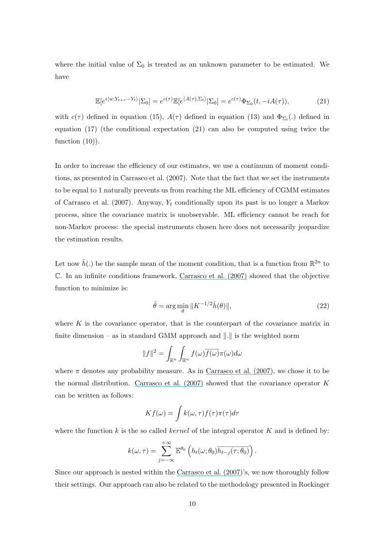
Let now h(.) be the sample mean of the moment condition, that is a function from R2n to
C. In an infinite conditions framework, Carrasco et al. (2007) showed that the objective
function to minimize is:
θ = arg minθ‖K−1/2h(θ)‖, (22)
where K is the covariance operator, that is the counterpart of the covariance matrix in
finite dimension – as in standard GMM approach and ‖.‖ is the weighted norm
‖f‖2 =∫
Rn
∫Rnf(ω)f(ω)π(ω)dω
where π denotes any probability measure. As in Carrasco et al. (2007), we chose it to be
the normal distribution. Carrasco et al. (2007) showed that the covariance operator K
can be written as follows:
Kf(ω) =∫k(ω, τ)f(τ)π(τ)dτ
where the function k is the so called kernel of the integral operator K and is defined by:
k(ω, τ) =+∞∑j=−∞
Eθ0(ht(ω; θ0)ht−j(τ ; θ0)
).
Since our approach is nested within the Carrasco et al. (2007)’s, we now thoroughly follow
their settings. Our approach can also be related to the methodology presented in Rockinger
10
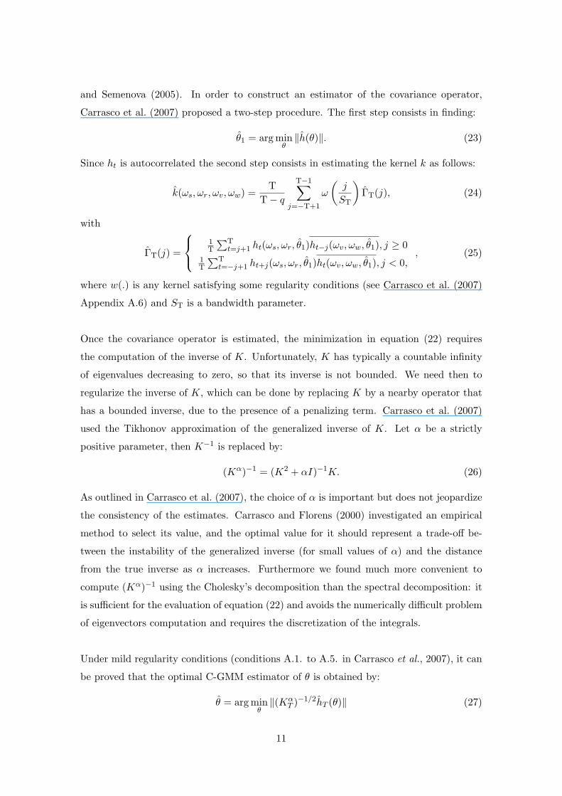
and Semenova (2005). In order to construct an estimator of the covariance operator,
Carrasco et al. (2007) proposed a two-step procedure. The first step consists in finding:
θ1 = arg minθ‖h(θ)‖. (23)
Since ht is autocorrelated the second step consists in estimating the kernel k as follows:
k(ωs, ωr, ωv, ωw) =T
T− q
T−1∑j=−T+1
ω
(j
ST
)ΓT(j), (24)
with
ΓT(j) =
1T
∑Tt=j+1 ht(ωs, ωr, θ1)ht−j(ωv, ωw, θ1), j ≥ 0
1T
∑Tt=−j+1 ht+j(ωs, ωr, θ1)ht(ωv, ωw, θ1), j < 0,
, (25)
where w(.) is any kernel satisfying some regularity conditions (see Carrasco et al. (2007)
Appendix A.6) and ST is a bandwidth parameter.
Once the covariance operator is estimated, the minimization in equation (22) requires
the computation of the inverse of K. Unfortunately, K has typically a countable infinity
of eigenvalues decreasing to zero, so that its inverse is not bounded. We need then to
regularize the inverse of K, which can be done by replacing K by a nearby operator that
has a bounded inverse, due to the presence of a penalizing term. Carrasco et al. (2007)
used the Tikhonov approximation of the generalized inverse of K. Let α be a strictly
positive parameter, then K−1 is replaced by:
(Kα)−1 = (K2 + αI)−1K. (26)
As outlined in Carrasco et al. (2007), the choice of α is important but does not jeopardize
the consistency of the estimates. Carrasco and Florens (2000) investigated an empirical
method to select its value, and the optimal value for it should represent a trade-off be-
tween the instability of the generalized inverse (for small values of α) and the distance
from the true inverse as α increases. Furthermore we found much more convenient to
compute (Kα)−1 using the Cholesky’s decomposition than the spectral decomposition: it
is sufficient for the evaluation of equation (22) and avoids the numerically difficult problem
of eigenvectors computation and requires the discretization of the integrals.
Under mild regularity conditions (conditions A.1. to A.5. in Carrasco et al., 2007), it can
be proved that the optimal C-GMM estimator of θ is obtained by:
θ = arg minθ‖(Kα
T )−1/2hT (θ)‖ (27)
11
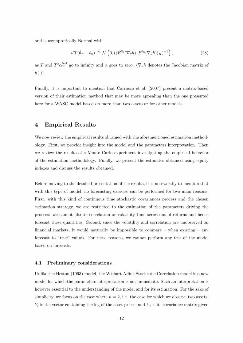
and is asymptotically Normal with
√T (θT − θ0) L→ N
(0, (〈Eθ0(∇θh), Eθ0(∇θh)〉K)−1
), (28)
as T and T aα5/4T go to infinity and α goes to zero. (∇θh denotes the Jacobian matrix of
h(.)).
Finally, it is important to mention that Carrasco et al. (2007) present a matrix-based
version of their estimation method that may be more appealing than the one presented
here for a WASC model based on more than two assets or for other models.
4 Empirical Results
We now review the empirical results obtained with the aforementioned estimation method-
ology. First, we provide insight into the model and the parameters interpretation. Then
we review the results of a Monte Carlo experiment investigating the empirical behavior
of the estimation methodology. Finally, we present the estimates obtained using equity
indexes and discuss the results obtained.
Before moving to the detailed presentation of the results, it is noteworthy to mention that
with this type of model, no forecasting exercise can be performed for two main reasons.
First, with this kind of continuous time stochastic covariances process and the chosen
estimation strategy, we are restricted to the estimation of the parameters driving the
process: we cannot filtrate correlation or volatility time series out of returns and hence
forecast these quantities. Second, since the volatility and correlation are unobserved on
financial markets, it would naturally be impossible to compare – when existing – any
forecast to ”true” values. For these reasons, we cannot perform any test of the model
based on forecasts.
4.1 Preliminary considerations
Unlike the Heston (1993) model, the Wishart Affine Stochastic Correlation model is a new
model for which the parameters interpretation is not immediate. Such an interpretation is
however essential to the understanding of the model and for its estimation. For the sake of
simplicity, we focus on the case where n = 2, i.e. the case for which we observe two assets.
Yt is the vector containing the log of the asset prices, and Σt is its covariance matrix given
12
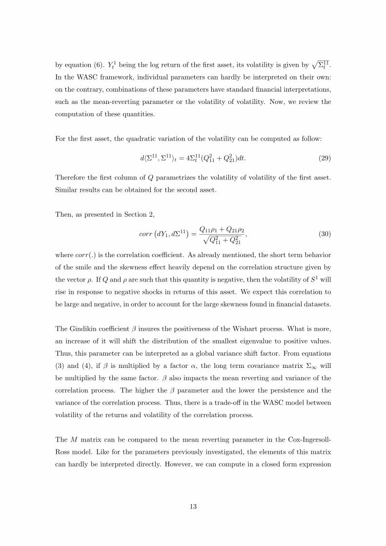
by equation (6). Y 1t being the log return of the first asset, its volatility is given by
√Σ11t .
In the WASC framework, individual parameters can hardly be interpreted on their own:
on the contrary, combinations of these parameters have standard financial interpretations,
such as the mean-reverting parameter or the volatility of volatility. Now, we review the
computation of these quantities.
For the first asset, the quadratic variation of the volatility can be computed as follow:
d〈Σ11,Σ11〉t = 4Σ11t (Q2
11 +Q221)dt. (29)
Therefore the first column of Q parametrizes the volatility of volatility of the first asset.
Similar results can be obtained for the second asset.
Then, as presented in Section 2,
corr(dY1, dΣ11
)=Q11ρ1 +Q21ρ2√
Q211 +Q2
21
, (30)
where corr(.) is the correlation coefficient. As already mentioned, the short term behavior
of the smile and the skewness effect heavily depend on the correlation structure given by
the vector ρ. If Q and ρ are such that this quantity is negative, then the volatility of S1 will
rise in response to negative shocks in returns of this asset. We expect this correlation to
be large and negative, in order to account for the large skewness found in financial datasets.
The Gindikin coefficient β insures the positiveness of the Wishart process. What is more,
an increase of it will shift the distribution of the smallest eigenvalue to positive values.
Thus, this parameter can be interpreted as a global variance shift factor. From equations
(3) and (4), if β is multiplied by a factor α, the long term covariance matrix Σ∞ will
be multiplied by the same factor. β also impacts the mean reverting and variance of the
correlation process. The higher the β parameter and the lower the persistence and the
variance of the correlation process. Thus, there is a trade-off in the WASC model between
volatility of the returns and volatility of the correlation process.
The M matrix can be compared to the mean reverting parameter in the Cox-Ingersoll-
Ross model. Like for the parameters previously investigated, the elements of this matrix
can hardly be interpreted directly. However, we can compute in a closed form expression
13
the drift part of the dynamics of Σij . In the case of the first asset:
dΣ11t = . . .+ Σ11
t
[2M11 + 2M12
√Σ22t√
Σ11t
ρ12t
]+ . . . , (31)
where ρ12t is the instantaneous correlation between the log-returns of the two assets. Thus,
the mean reverting parameter for Σ11 is a combination of the elements of M . What is
more, this drift term is made of two parts: a deterministic part (2M11) and a stochastic
correction (2M12
√Σ22t√
Σ11t
ρ12t ), linked to the joint dynamics of both assets. Thus, the drift
term of Σ11t is influenced by one of the off-diagonal elements of M . This feature cannot
be replicated by most of the multivariate GARCH-like models. We can perform similar
calculations for Σ12t and Σ22
t . These quantities can then be used to compare the half life
of the variances and covariance processes and thus evaluate their relative persistence in
financial markets.
The instantaneous correlation between assets has also a closed form expression:
dρ12t =
(At(ρ12t
)2 +Btρ12t + Ct
)dt+
√1−
(ρ12t
)2(...)d(Noiset) (32)
with At, Bt, Ct recursive functions of Σ11t , Σ22
t and the model parameters. We present the
drift coefficients and the diffusion term in the Appendix. The drift associated to the cor-
relation is quadratic, and the linear term has a negative coefficient Bt < 0, thus presenting
the typical mean reverting behavior of ρ12t (at least around zero where the quadratic part
is negligible). The linear part can thus be used to analyze the persistence of the correlation
and its mean-reverting characteristics, during low correlation periods. When the absolute
value of the correlation is higher, the quadratic part of the drift get the upper hand and
the correlation process looses most of its persistence. By comparing the values of Bt and
At, when can thus compare the correlation behavior during low and high correlation cy-
cles. This information has not been documented until now, whereas it is important to
understand the joint behavior of financial assets.
The WASC model can also be used to investigate potential contagion effects in financial
markets. By computing the correlation between the correlation process and the returns, we
can discuss under which condition the model is able to display an asymmetric correlation
effect3. Asymmetric correlation effect leads correlation to go up whilst returns are getting3On asymmetric correlation effects, see Roll (1988) and Ang and Chen (2002).
14
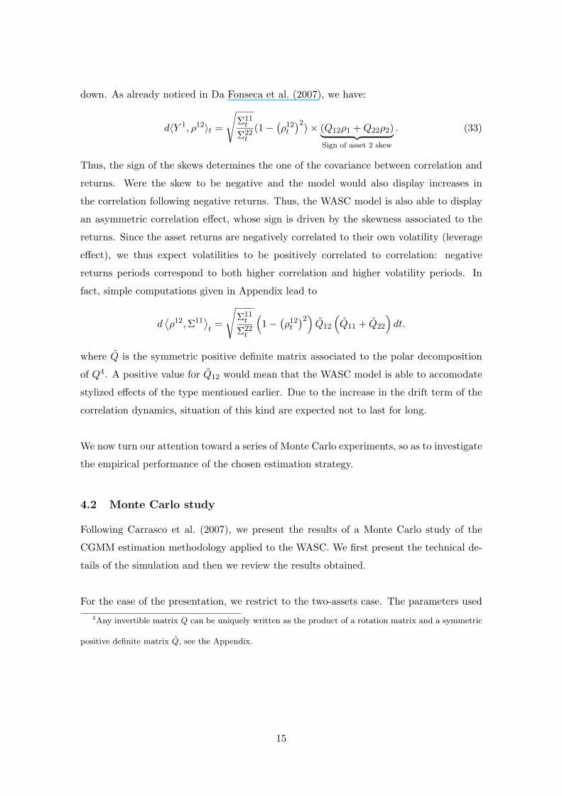
down. As already noticed in Da Fonseca et al. (2007), we have:
d〈Y 1, ρ12〉t =
√Σ11t
Σ22t
(1−(ρ12t
)2)× (Q12ρ1 +Q22ρ2)︸ ︷︷ ︸Sign of asset 2 skew
. (33)
Thus, the sign of the skews determines the one of the covariance between correlation and
returns. Were the skew to be negative and the model would also display increases in
the correlation following negative returns. Thus, the WASC model is also able to display
an asymmetric correlation effect, whose sign is driven by the skewness associated to the
returns. Since the asset returns are negatively correlated to their own volatility (leverage
effect), we thus expect volatilities to be positively correlated to correlation: negative
returns periods correspond to both higher correlation and higher volatility periods. In
fact, simple computations given in Appendix lead to
d⟨ρ12,Σ11
⟩t
=
√Σ11t
Σ22t
(1−
(ρ12t
)2)Q12
(Q11 + Q22
)dt.
where Q is the symmetric positive definite matrix associated to the polar decomposition
of Q4. A positive value for Q12 would mean that the WASC model is able to accomodate
stylized effects of the type mentioned earlier. Due to the increase in the drift term of the
correlation dynamics, situation of this kind are expected not to last for long.
We now turn our attention toward a series of Monte Carlo experiments, so as to investigate
the empirical performance of the chosen estimation strategy.
4.2 Monte Carlo study
Following Carrasco et al. (2007), we present the results of a Monte Carlo study of the
CGMM estimation methodology applied to the WASC. We first present the technical de-
tails of the simulation and then we review the results obtained.
For the ease of the presentation, we restrict to the two-assets case. The parameters used4Any invertible matrix Q can be uniquely written as the product of a rotation matrix and a symmetric
positive definite matrix Q, see the Appendix.
15
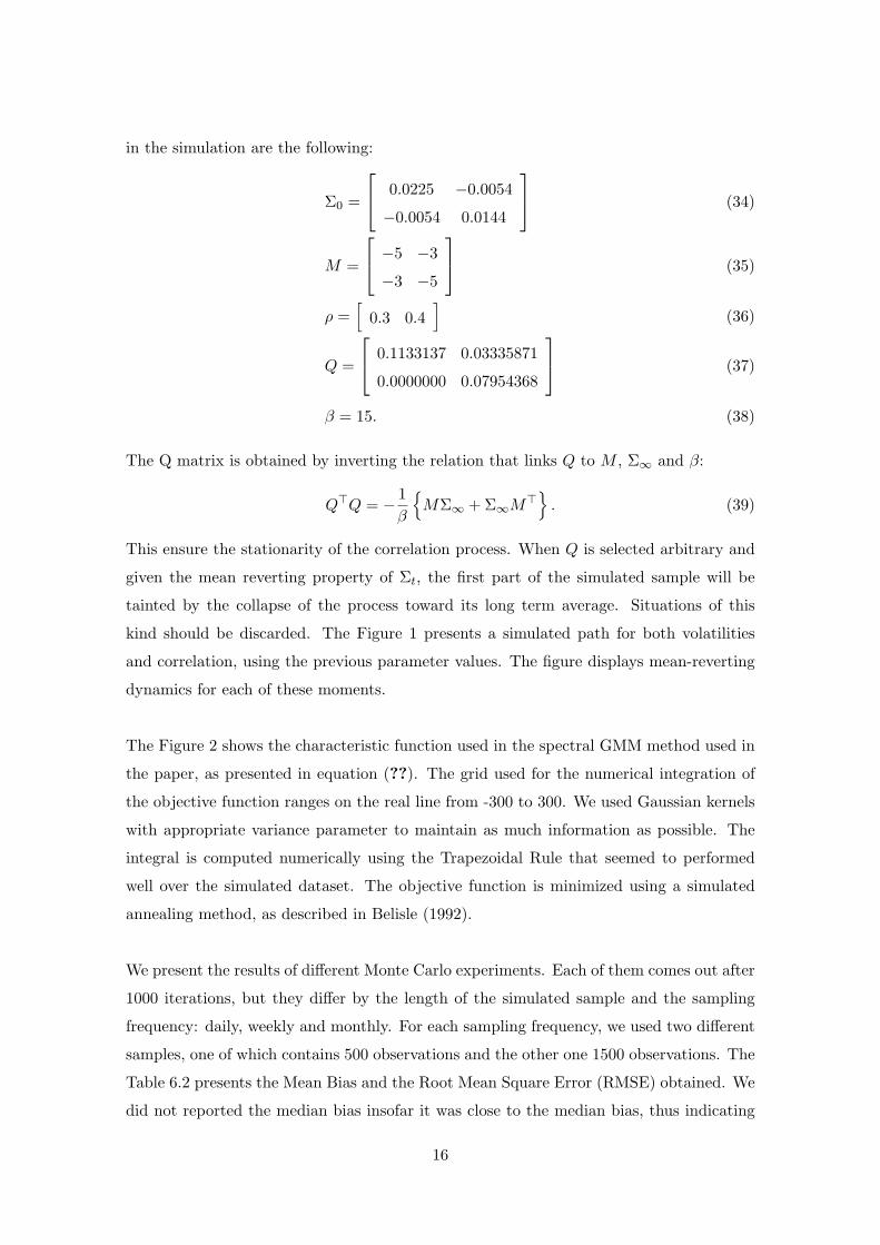
in the simulation are the following:
Σ0 =
0.0225 −0.0054
−0.0054 0.0144
(34)
M =
−5 −3
−3 −5
(35)
ρ =[
0.3 0.4]
(36)
Q =
0.1133137 0.03335871
0.0000000 0.07954368
(37)
β = 15. (38)
The Q matrix is obtained by inverting the relation that links Q to M , Σ∞ and β:
Q>Q = − 1β
MΣ∞ + Σ∞M>
. (39)
This ensure the stationarity of the correlation process. When Q is selected arbitrary and
given the mean reverting property of Σt, the first part of the simulated sample will be
tainted by the collapse of the process toward its long term average. Situations of this
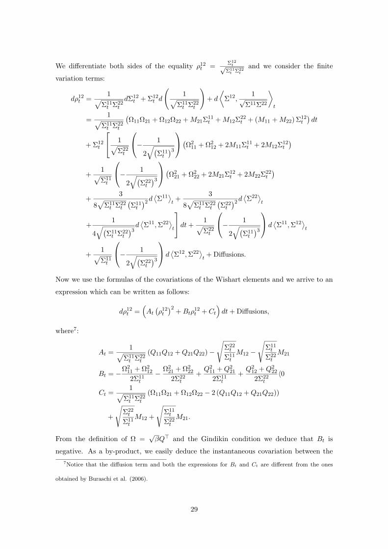
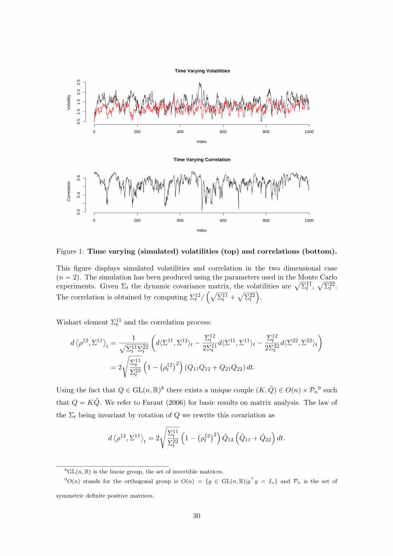
kind should be discarded. The Figure 1 presents a simulated path for both volatilities
and correlation, using the previous parameter values. The figure displays mean-reverting
dynamics for each of these moments.
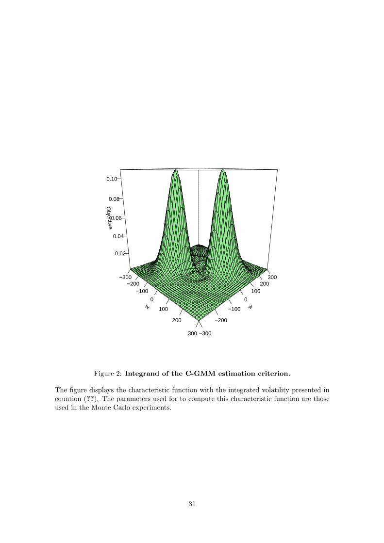
The Figure 2 shows the characteristic function used in the spectral GMM method used in
the paper, as presented in equation (??). The grid used for the numerical integration of
the objective function ranges on the real line from -300 to 300. We used Gaussian kernels
with appropriate variance parameter to maintain as much information as possible. The
integral is computed numerically using the Trapezoidal Rule that seemed to performed
well over the simulated dataset. The objective function is minimized using a simulated
annealing method, as described in Belisle (1992).
We present the results of different Monte Carlo experiments. Each of them comes out after
1000 iterations, but they differ by the length of the simulated sample and the sampling
frequency: daily, weekly and monthly. For each sampling frequency, we used two different
samples, one of which contains 500 observations and the other one 1500 observations. The
Table 6.2 presents the Mean Bias and the Root Mean Square Error (RMSE) obtained. We
did not reported the median bias insofar it was close to the median bias, thus indicating
16
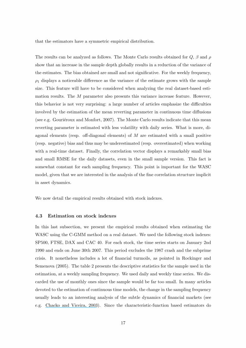
that the estimators have a symmetric empirical distribution.
The results can be analyzed as follows. The Monte Carlo results obtained for Q, β and ρ
show that an increase in the sample depth globally results in a reduction of the variance of
the estimates. The bias obtained are small and not significative. For the weekly frequency,
ρ1 displays a noticeable difference as the variance of the estimate grows with the sample
size. This feature will have to be considered when analyzing the real dataset-based esti-
mation results. The M parameter also presents this variance increase feature. However,
this behavior is not very surprising: a large number of articles emphasize the difficulties
involved by the estimation of the mean reverting parameter in continuous time diffusions
(see e.g. Gourieroux and Monfort, 2007). The Monte Carlo results indicate that this mean
reverting parameter is estimated with less volatility with daily series. What is more, di-
agonal elements (resp. off-diagonal elements) of M are estimated with a small positive
(resp. negative) bias and thus may be underestimated (resp. overestimated) when working
with a real-time dataset. Finally, the correlation vector displays a remarkably small bias
and small RMSE for the daily datasets, even in the small sample version. This fact is
somewhat constant for each sampling frequency. This point is important for the WASC
model, given that we are interested in the analysis of the fine correlation structure implicit
in asset dynamics.
We now detail the empirical results obtained with stock indexes.
4.3 Estimation on stock indexes
In this last subsection, we present the empirical results obtained when estimating the
WASC using the C-GMM method on a real dataset. We used the following stock indexes:
SP500, FTSE, DAX and CAC 40. For each stock, the time series starts on January 2nd
1990 and ends on June 30th 2007. This period excludes the 1987 crash and the subprime
crisis. It nonetheless includes a lot of financial turmoils, as pointed in Rockinger and
Semenova (2005). The table 2 presents the descriptive statistics for the sample used in the
estimation, at a weekly sampling frequency. We used daily and weekly time series. We dis-
carded the use of monthly ones since the sample would be far too small. In many articles
devoted to the estimation of continuous time models, the change in the sampling frequency
usually leads to an interesting analysis of the subtle dynamics of financial markets (see
e.g. Chacko and Viceira, 2003). Since the characteristic-function based estimators do
17
not suffer from discretization errors, we can actually use any sampling frequency. Like in
Carrasco et al. (2007), α = 0.02 were found to perform well. The integration grid is the
same as the one used for the previous simulation exercises. We chose to use the Bartlett
kernel for the GMM covariance matrix estimation, following the procedure presented in
Newey and West (1994).
For numerical sake, we focus again on a two-assets case (n = 2). We estimated the pa-
rameters driving the WASC process for the following couples of indexes: (SP500,FTSE),
(SP500,DAX), (SP500,CAC), (DAX/CAC), (DAX,FTSE) and (FTSE/DAX). This way,
we will be able to compare the characteristics specific to individual stock while estimated
with each of the others. For example, we will be able to compare the volatility of volatility
of the SP500, when it is estimated with the DAX, CAC and FTSE as a second asset. It
will highlight the impact of joint dynamics on idiosyncratic behaviors, which has hardly
be documented until now.
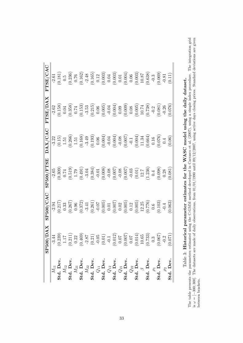
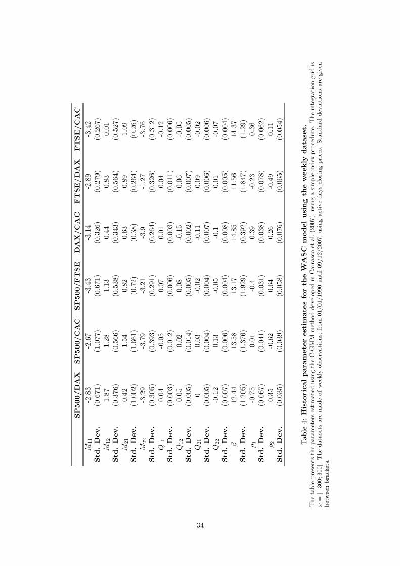
The estimation results are presented in table 3 for the daily results and in table 4 for the
weekly results. Most of the estimates are significative up to a 5 or 10% risk level. What
is more, in the weekly observation case, the size of the sample is strongly reduced and so
is the efficiency of the estimation method. Nevertheless, the estimation results yield in-
teresting information both about the WASC process and the dynamics of the stock indexes.
As presented in the previous subsection, it is difficult to compare the individual parameters
and we will thus focus on combinations of these parameters most of which are comparable
with the ones of the Heston (1993) model.
For the estimated parameters presented in Table 3, the associated volatility of volatility
are presented in Table 5. The estimation of this quantity is essential to test the ability
of the model to capture financial market features: as pointed out in Chacko and Viceira
(2003), this parameter controls the kurtosis of the underlying process. Several remarks can
be made. First, the global results match what is generally expected from stock indexes.
Such markets are known to lead to a volatility of volatility ranging from 5% to 25%.
Second, the results obtained for the SP500 are remarkably stable when the second asset
changes at least for the daily sample: it ranges from 14.6% to 24.4%, thus matching the
results obtained in Eraker et al. (2003). Still, it is below the estimates obtained in Chacko
and Viceira (2003) and Rockinger and Semenova (2005): this may be explained by the
18
fact that the model that is estimated here is multivariate, whereas existing attempts to
capture stochastic volatility has been made in a univariate framework. Da Fonseca et al.
(2007) showed that the correlation between the volatility of each stock is non 0 insofar as
d〈Σ11,Σ22〉 = Σ12dt. (40)
Hence, whenever Σ12 is positive, the WASC model is able to model volatility transmis-
sion phenomena among assets. It is noteworthy to remark that these results are globally
stable across the datasets and close to the existing results. Third, when the sampling
frequency reduces, the volatility of volatility parameter globally increases. The few lacks
of consistency for this fact may be due to the fact that the number of observations in the
weekly dataset is far below the one used in the daily dataset. These results are different
from those obtained in Chacko and Viceira (2003). However, this is in line with what is
observed for the volatility of the log-returns when reducing the sampling frequency. This
divergence may also be explained by the effect of the correlation between variances that
cannot be mimicked in a Heston-like framework.
Now, let us discuss an important parameter for the specification of the WASC model, that
is the correlation between the returns and the volatility. We already mentioned that this
parameter is essential to have a model that is consistent with many stylized facts, such as
negative skewness and thus skewed implied volatility surfaces. It can be computed using
its expression given in equation (30). The Table 6 displays the results obtained.
This time, we have results that are comparable to the one obtained in the existing liter-
ature, and especially for the SP500. The correlation for this index is reported in the first
line of the previous Table. In the literature, it actually ranges from -0.27 (Rockinger and
Semenova, 2005) to -0.62 (Chacko and Viceira, 2003), which is close to what is obtained
here. The parameter values obtained for the CAC, DAX and FTSE indexes are not sur-
prising either, since their sign is negative. The main problem here lies in the instability
of the ρ parameter for the different estimation involved, when comparing both the sample
frequency and the couple of indexes that are estimated. The change in sampling frequency
does not lead to a similar behavior across the datasets: depending upon the couples and
the sampling frequency, the skewness in the dataset can considerably differ, underlining
the fact that correlation processes implicit in financial markets are complex. Beyond the
remarks made in the previous paragraph on the importance of the dataset depth, we also
emphasize that the computation of this parameter dwells on the inverse of the square root
19
of a quantity that is small. In this situation, the inverse of something small can be found
to be very variable: any error in the estimation of Q11 and Q21 will have a strong impact
on 1√Q2
11+Q221
. Thus, this skewness quantity must be cautiously interpreted. Last but not
least, since the skews are negative, the fitted WASC models also display asymmetric cor-
relation effects: negative returns are likely to be followed by a higher correlation between
the two assets.
We now turn our attention toward the mean reverting matrix M . For SP500, CAC, DAX
and FTSE, we find the same structure for the matrix M . They are definite negative thus
ensuring a mean reverting behavior for the Wishart process and have positives off diagonal
terms. As presented in the previous subsection, the drift can be decomposed into two dif-
ferent part: an idiosyncratic part (denoted κ1 in the tables) and a joint part (denoted κ2 in
the tables). For univariate stochastic volatility models, the estimation results usually lead
to an estimate of κ = κ1 + κ2, that is the sum of the two preceding elements. Thanks to
the complexity of the WASC process, we are now able to disentangle and analyse these two
different elements. The estimation results are reported in table 7. The κ values should
be compared with the mean reverting value of the Heston. We are close to Rockinger
and Semenova (2005) results who found 6.3352 (see their Table 1) for the S&P500, even
though their results are obtained on a different sample and using daily data. However,
when analysing κ1 and κ2, we find that the idiosyncratic mean reverting component is
always higher than the usual Heston parameter. This idiosyncratic element is dampened
by the negative joint mean reverting component: its negativity is to be related to the
negative non-diagonal elements of the estimated M matrices. Again, when the sampling
frequency changes, each of these values vary, suggesting that the mean reverting parame-
ter associated to the volatility strongly depends on the sampling frequency, as pointed out
in Chacko and Viceira (2003). Globally, the associated half lives are around one month,
which is a realistic value.
As presented in the previous section, it is possible to perform similar computations for
the drift term of the stochastic correlation. This drift is a non linear function of ρ12t and
the usual comments have to be adapted. We present in figure 3 and 4 the instantaneous
variation of ρ12t as a function of ρ12
t , highlighting the contribution of the quadratic term
when the correlation gets very high – that is during crisis period. Our results suggest
that the correlation process is much more persistent than volatility when the correlation is
below its long term level, since in such a case its mean reverting parameter can be reduced
20
to (−Bt): in this situation, the half life is around 2 months, which is again realistic. When
correlation is high, the quadratic term gets higher and the persistence goes down, since
At is added to Bt as both these elements are negative. This is consistent with what is
empirically observed during financial market crises: the correlation gets very high on a
very short period, to finally go back to its long term behavior rapidly. The aforementioned
figures display reaction functions of this kind, underlining the ability of the WASC model
to encompass this standard feature of financial markets.
Another quantity of importance is ||ρ||, since the WASC can be seen as a generalization
of the processes proposed in Gourieroux and Sufana (2004) and Buraschi et al. (2006),
with a more complex correlation structure. Since the WASC model is only defined up to
a rotation matrix, the model presented in Buraschi et al. (2006) encompasses any correla-
tion structure that satisfies ||ρ|| = 1. Testing such an assumption is thus of a tremendous
importance to judge whether the complexity of the WASC is empirically justified. The
table 10 presents the norm of this vector parameter. Each of the estimated value strongly
differs from 1, suggesting the general correlation structure imposed in Da Fonseca et al.
(2007) is empirically grounded.
As presented earlier, a contagion effect can be handled by the WASC through a positive
value for Q12. In table 11 we report the estimated values for this parameter. We found
positive values for all couples of indexes as expected. Therefore, the estimated WASC
model is able to detect the existence of potential contagion effects in the dataset. As
mentioned earlier, these findings may be due to the fact that the dataset includes several
financial crises, periods during which dramatic contagion effects are expected.
5 Conclusion
In this paper we investigated the estimation of a new continuous time model: the Wishart
Affine Stochastic Correlation model, presented in Da Fonseca et al. (2007). After hav-
ing presented the problem that arise when trying to estimate a discrete version of this
model, this paper proposes to estimate the process using its exponential affine character-
istic function. The estimation method uses a continuum of spectral moment conditions
in a GMM framework. After a preliminary Monte Carlo investigation of the estimation
methodology, we show that real-dataset estimation results bring support to the WASC
21
process. First, the empirical results are comparable to those obtained in the literature
(when comparable). Second, the general correlation structure of the WASC casts light on
not-so-well documented features of international equities, allowing us to discuss for exam-
ple the persistence of the correlation process, contagion effects or asymmetric correlation
effects. Third, the generality of the correlation structure is not rejected by the dataset,
bringing empirical support to the model presented in Da Fonseca et al. (2007).
References
Ang, A. and Chen, J. (2002). Asymmetric Correlations of Equity Portfolios. Journal of
Financial Economic, (63):443–494.
Asai, M., McAleer, M., and Yu, J. (2006). Multivariate Stochastic Volatility: a Review.
Econometric Review, 25(2-3):145–175.
Bathia, R. (2005). Matrix Analysis. Graduate Texts in Mathematics, Springer-Verlag.
Bauwens, L., Laurent, S., and Rombouts, J. (2006). Multivariate garch models: a survey.
Journal of Applied Econometrics, 21(1):79–109.
Belisle, C. J. P. (1992). Convergence Theorems for a Class of Simulated Annealing Algo-
rithms. Rd J Applied Probability, 29:885–895.
Bru, M. F. (1991). Wishart Processes. Journal of Theoretical Probability, 4:725–743.
Buraschi, A., Porchia, P., and Trojani, F. (2006). Correlation risk and optimal portfolio
choice. Working paper, SSRN-908664.
Carrasco, M., Chernov, M., Florens, J.-P., and Ghysels, E. (2007). Efficient Estimation
of Jump Diffusions and General Dynamic Models with a Continuum of Moment Condi-
tions. Journal of Econometrics, (140):529–573.
Carrasco, M. and Florens, J. (2000). Generalization of GMM to a Continuum of Moment
Conditions. Econometric Theory, (16):797–834.
Chacko, G. and Viceira, L. M. (2003). Spectral GMM Estimation of Continuous-Time
Processes. Journal of Econometrics, 116(1-2):259–292.
Da Fonseca, J., Grasselli, M., and Tebaldi, C. (2007). Option Pricing when Correlations
are Stochastic: an Analytical Framework. Review of Derivatives Research, 10(2):151–
180.
22
Da Fonseca, J., Grasselli, M., and Tebaldi, C. (2008). A Multifactor Volatility Heston
Model,. Quantitative Finance, 8(6):591–604. An earlier version of this paper circulated
in 2005 as ”Wishart multi–dimensional stochastic volatility”, RR31, ESILV.
Daleckii, J. (1974). Differentiation of Non-Hermitian Matrix Functions Depending on a
Parameter. AMS Translations, 47(2):73–87.
Daleckii, J. and Krein, S. (1974). Integration and Differentiation of Functions of Hermitian
Operators and Applications to the Theory of Perturbations. AMS Translations, 47(2):1–
30.
Donoghue, W. J. (1974). Monotone matrix functions and analytic continuation. Springer-
Verlag.
Duffie, D. and Singleton, K. (1993). Simulated Moments Estimation of Markov Models of
Asset Prices. Econometrica, 61:929–952.
Eraker, B., Johannes, M., and Polson, N. (2003). The Impact of Jumps in Volatility and
Returns. The Journal of Finance, 58(3):1269–1300.
Faraut, J. (2006). Analyse sur les groupes de Lie. Calvage & Mounet.
Gourieroux, C. (2006). Continuous Time Wishart Process for Stochastic Risk. Econometric
Review, 25(2-3):177–217.
Gourieroux, C. and Jasiak, J. (2001). Financial Econometrics. Princeton University Press.
Gourieroux, C. and Sufana, R. (2004). Derivative Pricing with Multivariate Stochastic
Volatility: Application to Credit Risk. Les Cahiers du CREF 04-09.
Hall, B. C. (2003). Lie Groups, Lie Algebras, and Representations: An Elementary intro-
duction. Graduate Texts in Mathematics 222, Springer-Verlag.
Heston, S. (1993). A Closed-Form Solution for Options with Stochastic Volatility with
Applications to Bond and Currency Options. The Review of Financial Studies, 6(2).
Jiang, G. J. and Knight, J. L. (2002). Estimation of Continuous-Time Processes via
the Empirical Characteristic Function. Journal of Business & Economic Statistics,
20(2):198–212.
Lo, A. W. (1988). Maximum Likelihood Estimation of Generalized Ito Processes with
Discretely Sampled Data. Econometric Theory, 4:231–247.
23
Newey, W. K. and West, K. D. (1994). Automatic lag selection in covariance matrix
estimation. Review of Economic Studies, 61(4):631–53.
Rockinger, M. and Semenova, M. (2005). Estimation of Jump-Diffusion Process via Empir-
ical Characteristic Function. FAME Research Paper Series rp150, International Center
for Financial Asset Management and Engineering.
Roll, R. (1988). The International Crash of October, 1987. Financial Analysts Journal,
(September-October):19–35.
Singleton, K. (2001). Estimation of Affine Pricing Models Using the Empirical Character-
istic Function. Journal of Econometrics, (102):111–141.
Singleton, K. J. (2006). Empirical Dynamic Asset Pricing: Model Specification and Econo-
metric Assessment. Princeton University Press.
24
6 Appendix
6.1 Computing the gradient
The gradient of the characteristic function is needed to study the asymptotic distribution
of the estimates but also in the optimization process underlying the estimation procedure.
Therefore we turn our attention to the differentiation of matrix function depending on a
parameter. We illustrate the theoretical framework with the characteristic function of the
assets’ log returns and we give without technical details the results for the forward char-
acteristic function needed in our empirical study. We mainly rely on the work of Daleckii
(1974) for the general case (i.e. in the non-Hermitian matrix case) and to Daleckii and
Krein (1974), Donoghue (1974) and Bathia (2005) for the Hermitian matrix case.
Let us first state some basic results on linear algebra. Denote by λi; i = 1..n the set of
eigenvalues of a matrix X ∈Mn and mi the multiplicity of λi as a root of the characteristic
polynomial of X. Define Li = Ker(X − λiI) and Pi the projection operator from Cn onto
Li, then we have∑n
i=1 Pi = I. Define also Ji such that (X − λiI)Pi = Ji. The Jordan
normal form of X if given by the well known decomposition X =∑n
i=1(λiPi + Ji).
Let f be a function from Mn into Mn: the derivative of f at X in direction H, denoted
Df,X(H), is by definition ‖f(X+tH)−f(X)−Df,X(H)‖ = to(‖H‖) and can be computed
using the following formula Daleckii (1974):
Df,X(H) =n∑
j1,j2
mj1−1∑r1=0
mj2−1∑r2=0
1r1r2
∂r1+r2
∂λr1j1∂λr2j2
[f(λj1)− f(λj2)
λj1 − λj2
]Pj1J
r1j1HPj2J
r2j2. (41)
Remark 6.1. Whenever λj1 = λj2 the term within the bracket should be replaced by
f ′(λj1).
Remark 6.2. When X can be diagonalized then mj = 1 for each j and we are lead to the
very simple form
Df,X(H) =n∑
j1,j2
[f(λj1)− f(λj2)
λj1 − λj2
]Pj1HPj2 . (42)
If X is Hermitian then P−1 = P ∗ and we recover the result presented for example in
Daleckii and Krein (1974).
25
Simple algebra leads to Df,X(H) = PMf (P−1HP )P−1 where P is the matrix of the
eigenvectors of X5, is the Schur product6 and Mf = (Mf (λk, λl))k=1...n,l=1...n is the
Pick matrix associated to the function f , which is defined by
Mf (λ, µ) =
f(λ)−f(µ)
λ−µ if λ 6= µ
f ′(λ) if λ = µ(43)
This formulation is well known and can be found for example in Donoghue (1974) p. 79
and Bathia (2005) p123-124.
The gradient of the characteristic function involves ∂αA where A is given by (13). In fact
for any parameter value α which may be equal to Mkl, Qkl, Rkl or β the gradient is given
by
∂αΦYt,Σt(τ, z) = (Tr(∂αAΣt) + ∂αc(τ)) ΦYt,Σt(τ, z).
From (13) and ∂α(L−1) = −L−1(∂αL)L−1 implied by the derivation of L−1L = I we
conclude that
∂αA (τ) = −A22 (τ)−1 ∂α(A22 (τ))A(τ) +A22(τ)−1∂αA21 (τ) ,
Therefore we are lead to the computation of ∂αA11 (τ) ∂αA12 (τ)
∂αA21 (τ) ∂αA22 (τ)
,
that is the derivative with respect to a parameter of a function of a matrix (in this case
the exponential function). In order to use formula (41) we specify in the following table
for each parameter of the WASC model the choice of the matrice X and H. As usual
el; l = 1 . . . n resp. ekl; k, l = 1 . . . n stands for the canonical basis of Rn resp. Mn(R)
(the function f being f(x) = ex).
Parameter X H
Mkl τG τ
ekl 0
0 −ekl>
Qij τG τ
(ekl)>ρiω> −2(Q>ekl + (ekl)>Q)
0 −iωρ>ekl
ρl τG τ
Q>eliω> 0
0 −iωe>l Q
5If pi is the ith eigenvector of X and qi is the ith row of P−1 then the projection operator on Li is given
by Pi = piq>i
6Given two matrix of same size Xkl and Y kl then X Y = XklY kl
26
To fulfill the analytical computation of the gradient we need the derivative of c(τ) with
respect to a model parameter and particularly the term logA22(τ).
∂αc(τ) = −β2
[Tr (∂α(logA22(τ))) + τTr
(∂αM
> + iω∂α(ρ>Q))]
(44)
In order to apply (41) we just need to define P22 from M2n into Mn such that P22L = L22
with
L =
L11 L12
L21 L22
. (45)
Then it is easy to see that
∂α logA22(τ) = Dlog,A22(τ)(P22Dexp,τG(H)) (46)
Once again using (41) with the log function gives the result.
Remark 6.3. If f is the exponential function then we can also compute the derivative of
the exponential of a matrix using the Baker-Hausdorff’s formula (see e.g. Hall (2003) p.
71 formula (3.10) for the details)
∂αeτG = D expτG ∂α(τG), (47)
where D expX = eX I−e−adX
adXand adXY = [X,Y ] = XY − Y X is the Lie bracket.
The empirical study is based on the forward characteristic function of assets’ log returns
defined by
ΦΣ0(t,−iA(τ))ec(τ) = exp Tr [B(t)Σ0] + C(t) + c(τ) (48)
with
B (t) = (A(τ)B12(t) +B22(t))−1(A(τ)B11(t) +B21(t))
C(t) = −β2
Tr[log(A(τ)B12(t) +B22(t)) + tM>
]c(τ) = −β
2Tr[log(A22(τ)) + τM> + τiγ(ρ>Q)
]As for the characteristic function of assets’ log returns it is straightforward to show that
for any given model parameter α we have:
∂αΦΣ0(t,−iA(τ))ec(τ) = ΦΣ0(t,−iA(τ))ec(τ) (Tr(∂αB(t)Σ0) + ∂αC(t) + ∂αc(τ)))
27
where the matrix derivatives are given by
∂αB(t) = −(A(τ)B12(t) +B22(t))(∂αA(τ)B12(t) +A(τ)∂αB12(t) + ∂αB22(t))−1B(t)
+ (A(τ)B12(t) +B22(t))−1(∂αA(τ)B11(t) +B21(t)),
∂αC(t) = −β2
Tr(Dlog,A(τ)B12(t)+B22(t)(∂αA(τ)B12(t) +A(τ)∂αB12(t) + ∂αB22(t))).
This completes the analytical computation of the gradient.
6.2 Dynamics of the correlation process
In this Appendix we compute in the 2-dimensional case the drift and the diffusion coeffi-
cients of the correlation process ρ12t defined by
ρ12t =
Σ12t√
Σ11t Σ22
t
. (49)
We differentiate both sides of the equality(ρ12t
)2 = (Σ12t )2
Σ11t Σ22
t. We refer to Da Fonseca et al.
(2008) for the explicit computation of all covariations involved in the below formulas. We
obtain:
2ρ12t dρ
12t =
2Σ12t
Σ11t Σ22
t
dΣ12t +
(Σ12t
)2( 1Σ22t
d
(1
Σ11t
)+
1Σ11t
d
(1
Σ22t
))+ (.)dt,
so that
dρ12t =
1√Σ11t Σ22
t
(dΣ12
t −Σ12t
2Σ11t
dΣ11t −
Σ12t
2Σ22t
dΣ22t
)+ (.)dt.
By using the covariations among the Wishart elements we have
d⟨ρ12⟩t
=1
Σ11t Σ22
t
[Σ11t
(Q2
12 +Q222
)+ 2Σ12
t (Q11Q12 +Q21Q22) + Σ22t
(Q2
11 +Q221
)+(Σ12t
)2(Q211 +Q2
21
Σ11t
+Q2
12 +Q222
Σ22t
+ 2Σ12t
Σ11t Σ22
t
(Q11Q12 +Q21Q22))
− 2Σ12t
Σ11t
(Σ11t (Q11Q12 +Q21Q22) + Σ12
t
(Q2
11 +Q221
))−2
Σ12t
Σ22t
(Σ12t
(Q2
12 +Q222
)+ Σ22
t (Q11Q12 +Q21Q22))]dt,
which leads to:
d⟨ρ12⟩t
=(
1−(ρ12t
)2)(Q212 +Q2
22
Σ22t
+Q2
11 +Q221
Σ11t
− 2ρ12t (Q11Q12 +Q21Q22)√
Σ11t Σ22
t
)dt.
Now let us compute the drift of the process ρ12t .
28
We differentiate both sides of the equality ρ12t = Σ12
t√Σ11t Σ22
t
and we consider the finite
variation terms:
dρ12t =
1√Σ11t Σ22
t
dΣ12t + Σ12
t d
(1√
Σ11t Σ22
t
)+ d
⟨Σ12,
1√Σ11Σ22
⟩t
=1√
Σ11t Σ22
t
(Ω11Ω21 + Ω12Ω22 +M21Σ11
t +M12Σ22t + (M11 +M22) Σ12
t
)dt
+ Σ12t
1√Σ22t
− 1
2√(
Σ11t
)3(Ω2
11 + Ω212 + 2M11Σ11
t + 2M12Σ12t
)
+1√Σ11t
− 1
2√(
Σ22t
)3(Ω2
21 + Ω222 + 2M21Σ12
t + 2M22Σ22t
)+
3
8√
Σ11t Σ22
t
(Σ11t
)2d ⟨Σ11⟩t+
3
8√
Σ11t Σ22
t
(Σ22t
)2d ⟨Σ22⟩t
+1
4√(
Σ11t Σ22
t
)3d ⟨Σ11,Σ22⟩t
dt+1√Σ22t
− 1
2√(
Σ11t
)3 d
⟨Σ11,Σ12
⟩t
+1√Σ11t
− 1
2√(
Σ22t
)3 d
⟨Σ12,Σ22
⟩t+ Diffusions.
Now we use the formulas of the covariations of the Wishart elements and we arrive to an
expression which can be written as follows:
dρ12t =
(At(ρ12t
)2 +Btρ12t + Ct
)dt+ Diffusions,
where7:
At =1√
Σ11t Σ22
t
(Q11Q12 +Q21Q22)−
√Σ22t
Σ11t
M12 −
√Σ11t
Σ22t
M21
Bt = −Ω211 + Ω2
12
2Σ11t
− Ω221 + Ω2
22
2Σ22t
+Q2
11 +Q221
2Σ11t
+Q2
12 +Q222
2Σ22t
〈0
Ct =1√
Σ11t Σ22
t
(Ω11Ω21 + Ω12Ω22 − 2 (Q11Q12 +Q21Q22))
+
√Σ22t
Σ11t
M12 +
√Σ11t
Σ22t
M21.
From the definition of Ω =√βQ> and the Gindikin condition we deduce that Bt is
negative. As a by-product, we easily deduce the instantaneous covariation between the7Notice that the diffusion term and both the expressions for Bt and Ct are different from the ones
obtained by Buraschi et al. (2006).
29
0 200 400 600 800 1000
0.5
1.0
1.5
2.0
2.5
Index
Vol
atili
tyTime Varying Volatilities
0 200 400 600 800 1000
0.0
0.4
0.8
Index
Cor
rela
tion
Time Varying Correlation
Figure 1: Time varying (simulated) volatilities (top) and correlations (bottom).
This figure displays simulated volatilities and correlation in the two dimensional case(n = 2). The simulation has been produced using the parameters used in the Monte Carloexperiments. Given Σt the dynamic covariance matrix, the volatilities are
√Σ11t ,√
Σ22t .
The correlation is obtained by computing Σ12t /(√
Σ11t +
√Σ22t
).
Wishart element Σ11t and the correlation process:
d⟨ρ12,Σ11
⟩t
=1√
Σ11t Σ22
t
(d〈Σ11,Σ12〉t −
Σ12t
2Σ11t
d〈Σ11,Σ11〉t −Σ12t
2Σ22t
d〈Σ22,Σ22〉t)
= 2
√Σ11t
Σ22t
(1−
(ρ12t
)2) (Q11Q12 +Q21Q22) dt.
Using the fact that Q ∈ GL(n,R)8 there exists a unique couple (K, Q) ∈ O(n)×Pn9 such
that Q = KQ. We refer to Faraut (2006) for basic results on matrix analysis. The law of
the Σt being invariant by rotation of Q we rewrite this covariation as
d⟨ρ12,Σ11
⟩t
= 2
√Σ11t
Σ22t
(1−
(ρ12t
)2)Q12
(Q11 + Q22
)dt.
8GL(n,R) is the linear group, the set of invertible matrices.9O(n) stands for the orthogonal group ie O(n) = g ∈ GL(n,R)|g>g = In and Pn is the set of
symmetric definite positive matrices.
30
w
−300−200
−100
0
100
200
300
w
−300
−200
−100
0
100200
300O
bjective
0.02
0.04
0.06
0.08
0.10
Figure 2: Integrand of the C-GMM estimation criterion.
The figure displays the characteristic function with the integrated volatility presented inequation (??). The parameters used for to compute this characteristic function are thoseused in the Monte Carlo experiments.
31
Daily Weekly
Number of obs. 500 1500 500 1500
M11 Bias 0.0133 0.0382 0.227 0.0706RMSE 1.5126 1.5213 1.529 1.6011
M12 Bias -0.04 -0.014 -0.048 -0.036RMSE 1.0136 1.0341 1.098 1.0896
M21 Bias -0.056 -0.04 -0.085 -0.036RMSE 0.981 1.0205 1.104 1.1101
M22 Bias 0.1667 0.1784 0.070 0.0657RMSE 1.5378 1.5502 1.511 1.5778
Q11 Bias 0.1077 0.1069 0.132 0.1166RMSE 0.088 0.0872 0.476 0.3568
Q12 Bias 0.0309 0.0287 0.022 0.0208RMSE 0.0664 0.0675 0.554 0.4467
Q21 Bias -3E-04 -6E-04 -0.059 -0.008RMSE 0.0876 0.0862 0.553 0.371
Q22 Bias 0.0792 0.0772 0.057 0.0574RMSE 0.0678 0.0661 0.455 0.4424
β Bias 0.0632 -0.066 0.044 -0.107RMSE 4.335 4.3472 4.546 4.4364
ρ1 Bias 0.0055 -0.007 0.035 0.0268RMSE 0.4617 0.4913 0.641 0.8031
ρ2 Bias -0.004 0.0265 0.063 0.0445RMSE 0.5231 0.4734 0.653 0.6405
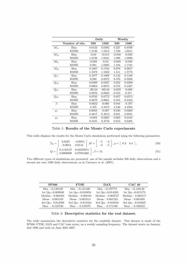
Table 1: Results of the Monte Carlo experiments
This table displays the results for the Monte Carlo simulations performed using the following parameters:
Σ0 =
[0.0225 −0.0054−0.0054 0.0144
].M =
[−5 −3−3 −5
], ρ =
[0.3 0.4
], (50)
Q =
[0.1133137 0.033358710.0000000 0.07954368
], β = 15. (51)
Two different types of simulations are presented: one of the sample includes 500 daily observations and asecond one uses 1500 daily observations, as in Carrasco et al. (2007).
SP500 FTSE DAX CAC 40
Min. :-0.128129 Min. :-0.141420 Min. :-0.197775 Min. :-0.1491491st Qu.:-0.009940 1st Qu.:-0.010858 1st Qu.:-0.014283 1st Qu.:-0.015173Median : 0.002491 Median : 0.002101 Median : 0.003727 Median : 0.002117Mean : 0.001535 Mean : 0.001014 Mean : 0.001523 Mean : 0.001095
3rd Qu.: 0.013506 3rd Qu.: 0.013424 3rd Qu.: 0.019416 3rd Qu.: 0.018025Max. : 0.123746 Max. : 0.135879 Max. : 0.171546 Max. : 0.166252
Table 2: Descriptive statistics for the real dataset.
The table summarizes the descriptive statistics for the available dataset. This dataset is made of theSP500, FTSE, DAX and CAC time series, on a weekly sampling frequency. The dataset starts on January2nd 1990 and ends on June 30th 2007.
32
SP
500/
DA
XS
P50
0/C
AC
SP
500/
FT
SE
DA
X/C
AC
FT
SE
/DA
XF
TS
E/C
AC
M11
-3.4
4-2
.94
-2.6
5-3
.22
-2.6
2-2
.61
Std
.D
ev.
(0.2
39)
(0.2
17)
(0.3
09)
(0.1
5)(0
.158
)(0
.181
)M
12
1.17
0.33
0.74
1.51
0.04
0.5
Std
.D
ev.
(0.2
11)
(0.2
67)
(0.5
19)
(0.2
66)
(0.3
58)
(0.2
36)
M21
0.22
0.96
1.79
1.51
0.74
0.76
Std
.D
ev.
(0.4
69)
(0.3
72)
(0.4
91)
(0.1
68)
(0.1
53)
(0.1
62)
M22
-2.8
7-3
.41
-3.0
4-3
.49
-3.5
3-2
.48
Std
.D
ev.
(0.2
1)(0
.261
)(0
.384
)(0
.193
)(0
.215
)(0
.165
)Q
11
-0.0
5-0
.07
-0.0
10.
060.
060.
12S
td.
Dev
.(0
.01)
(0.0
05)
(0.0
08)
(0.0
04)
(0.0
05)
(0.0
03)
Q12
-0.1
0.01
-0.0
8-0
.04
-0.0
40.
04S
td.
Dev
.(0
.012
)(0
.007
)(0
.007
)(0
.004
)(0
.004
)(0
.003
)Q
21
0.07
0.02
-0.0
8-0
.08
0.09
0.01
Std
.D
ev.
(0.0
07)
(0.0
05)
(0.0
07)
(0.0
07)
(0.0
09)
(0.0
04)
Q22
0.07
0.12
-0.0
3-0
.10.
080.
06S
td.
Dev
.(0
.014
)(0
.005
)(0
.01)
(0.0
04)
(0.0
05)
(0.0
03)
β10
.65
12.2
512
.711
.34
10.7
410
.87
Std
.D
ev.
(0.7
33)
(0.7
76)
(1.2
36)
(0.6
64)
(0.7
38)
(0.6
38)
ρ1
0.3
0.6
0.4
0.16
-0.2
-0.3
Std
.D
ev.
(0.0
67)
(0.1
03)
(0.0
98)
(0.0
76)
(0.0
81)
(0.0
69)
ρ2
-0.2
-0.4
0.28
0.4
-0.2
6-0
.81
Std
.D
ev.
(0.0
71)
(0.0
63)
(0.0
81)
(0.0
6)(0
.076
)(0
.11)
Tab
le3:
His
tori
cal
par
amet
eres
tim
ates
for
the
WA
SC
mod
elu
sin
gth
ed
aily
dat
aset
.T
he
table
pre
sents
the
para
met
ers
esti
mate
dusi
ng
the
C-G
MM
met
hod
dev
elop
edin
Carr
asc
oet
al.
(2007),
usi
ng
asi
mple
index
pro
cedure
.T
he
inte
gra
tion
gri
disω
=[−
300;3
00].
The
data
sets
are
made
of
daily
obse
rvati
ons,
from
01/01/1990
unti
l09/12/2007,
usi
ng
act
ive
day
scl
osi
ng
pri
ces.
Sta
ndard
dev
iati
ons
are
giv
enb
etw
een
bra
cket
s.
33
SP
500/
DA
XS
P50
0/C
AC
SP
500/
FT
SE
DA
X/C
AC
FT
SE
/DA
XF
TS
E/C
AC
M11
-2.8
3-2
.67
-3.4
3-3
.14
-2.8
9-3
.42
Std
.D
ev.
(0.6
71)
(1.0
77)
(0.6
71)
(0.3
26)
(0.2
79)
(0.2
67)
M12
1.87
1.28
1.13
0.44
0.83
0.01
Std
.D
ev.
(0.3
76)
(0.5
66)
(0.5
38)
(0.3
43)
(0.5
64)
(0.5
27)
M21
0.42
1.54
0.82
0.63
0.89
1.09
Std
.D
ev.
(1.0
02)
(1.6
61)
(0.7
2)(0
.38)
(0.2
64)
(0.2
6)M
22
-3.2
9-3
.79
-3.2
1-3
.9-1
.27
-3.7
6S
td.
Dev
.(0
.305
)(0
.393
)(0
.291
)(0
.264
)(0
.326
)(0
.312
)Q
11
0.04
-0.0
50.
070.
010.
04-0
.12
Std
.D
ev.
(0.0
03)
(0.0
12)
(0.0
06)
(0.0
03)
(0.0
11)
(0.0
06)
Q12
0.05
0.02
0.08
-0.1
50.
06-0
.05
Std
.D
ev.
(0.0
05)
(0.0
14)
(0.0
05)
(0.0
02)
(0.0
07)
(0.0
05)
Q21
00.
03-0
.02
-0.1
10.
09-0
.02
Std
.D
ev.
(0.0
05)
(0.0
04)
(0.0
04)
(0.0
07)
(0.0
06)
(0.0
06)
Q22
-0.1
20.
13-0
.05
-0.1
0.01
-0.0
7S
td.
Dev
.(0
.007
)(0
.006
)(0
.004
)(0
.008
)(0
.005
)(0
.004
)β
12.4
413
.58
13.1
714
.85
11.5
614
.37
Std
.D
ev.
(1.2
05)
(1.3
76)
(1.9
29)
(0.3
92)
(1.8
47)
(1.2
9)ρ
1-0
.75
0.01
-0.4
0.39
-0.2
30.
36S
td.
Dev
.(0
.067
)(0
.041
)(0
.031
)(0
.038
)(0
.078
)(0
.062
)ρ
20.
35-0
.62
0.64
0.26
-0.4
90.
11S
td.
Dev
.(0
.035
)(0
.039
)(0
.058
)(0
.076
)(0
.065
)(0
.054
)
Tab
le4:
His
tori
cal
par
amet
eres
tim
ates
for
the
WA
SC
mod
elu
sin
gth
ew
eekly
dat
aset
.T
he
table
pre
sents
the
para
met
ers
esti
mate
dusi
ng
the
C-G
MM
met
hod
dev
elop
edin
Carr
asc
oet
al.
(2007),
usi
ng
asi
mple
index
pro
cedure
.T
he
inte
gra
tion
gri
dis
ω=
[−300;3
00].
The
data
sets
are
made
of
wee
kly
obse
rvati
ons,
from
01/01/1990
unti
l09/12/2007,
usi
ng
act
ive
day
scl
osi
ng
pri
ces.
Sta
ndard
dev
iati
ons
are
giv
enb
etw
een
bra
cket
s.
34
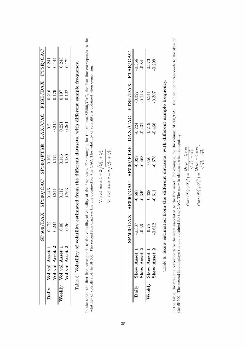
SP
500/
DA
XS
P50
0/C
AC
SP
500/
FT
SE
DA
X/C
AC
FT
SE
/DA
XF
TS
E/C
AC
Dai
lyV
olvo
lA
sset
10.
172
0.14
60.
161
0.2
0.21
60.
241
Vol
vol
Ass
et2
0.24
40.
241
0.17
10.
215
0.17
90.
144
Wee
kly
Vol
vol
Ass
et1
0.08
0.11
70.
146
0.22
10.
197
0.24
3V
olvo
lA
sset
20.
260.
263
0.18
90.
361
0.12
20.
172
Tab
le5:
Vol
atilit
yof
vola
tility
esti
mat
edfr
omth
ed
iffer
ent
dat
aset
s,w
ith
diff
eren
tsa
mp
lefr
equ
ency
.
Inth
eta
ble
,th
efirs
tline
corr
esp
onds
toth
evola
tility
of
vola
tility
of
the
firs
tass
et.
For
exam
ple
,fo
rth
eco
lum
nSP
500/C
AC
,th
efirs
tline
corr
esp
onds
toth
evola
tility
of
vola
tility
of
the
SP
500.
The
seco
nd
line
dis
pla
ys
the
one
obta
ined
for
the
CA
C.
The
vola
tility
of
vola
tility
isobta
ined
when
com
puti
ng:
Vol/
vol
Ass
et1
=2√ Q
2 11
+Q
2 21
Vol/
vol
Ass
et2
=2√ Q
2 12
+Q
2 22.
SP
500/
DA
XS
P50
0/C
AC
SP
500/
FT
SE
DA
X/C
AC
FT
SE
/DA
XF
TS
E/C
AC
Dai
lyS
kew
Ass
et1
-0.3
37-0
.687
-0.3
27-0
.224
-0.3
27-0
.366
Ske
wA
sset
2-0
.36
-0.3
49-0
.468
-0.4
31-0
.143
-0.8
4W
eekly
Ske
wA
sset
1-0
.75
-0.3
28-0
.56
-0.2
19-0
.541
-0.3
73S
kew
Ass
et2
-0.6
12-0
.611
-0.6
78-0
.466
-0.3
07-0
.299
Tab
le6:
Ske
wes
tim
ated
from
the
diff
eren
td
atas
ets,
wit
hd
iffer
ent
sam
ple
freq
uen
cy.
Inth
eta
ble
,th
efirs
tline
corr
esp
onds
toth
esk
ewass
oci
ate
dto
the
firs
tass
et.
For
exam
ple
,fo
rth
eco
lum
nSP
500/C
AC
,th
efirs
tline
corr
esp
onds
toth
esk
ewof
the
SP
500.
The
seco
nd
line
dis
pla
ys
the
one
obta
ined
for
the
CA
C.
The
skew
isobta
ined
when
com
puti
ng:
Corr( dY
1 t,d
Σ11t
) =Q
11ρ1
+Q
21ρ2
√ Q2 11
+Q
2 21
Corr( dY
2 t,d
Σ22t
) =Q
12ρ1
+Q
22ρ2
√ Q2 12
+Q
2 22
.
35
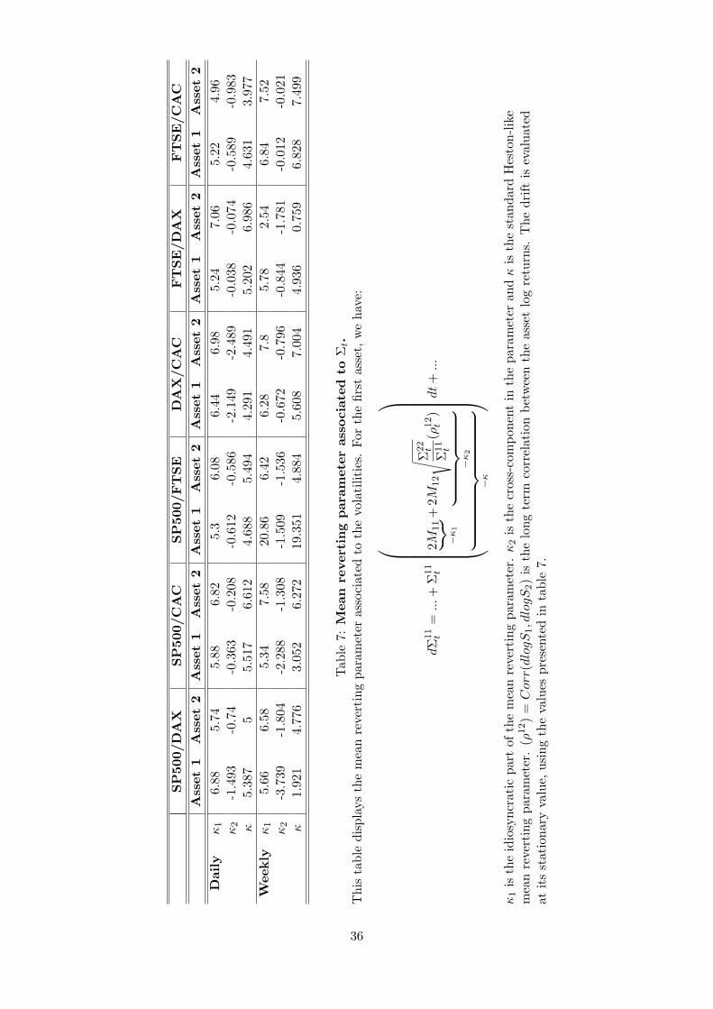
SP
500/
DA
XS
P50
0/C
AC
SP
500/
FT
SE
DA
X/C
AC
FT
SE
/DA
XF
TS
E/C
AC
Ass
et1
Ass
et2
Ass
et1
Ass
et2
Ass
et1
Ass
et2
Ass
et1
Ass
et2
Ass
et1
Ass
et2
Ass
et1
Ass
et2
Dai
lyκ
16.
885.
745.
886.
825.
36.
086.
446.
985.
247.
065.
224.
96κ
2-1
.493
-0.7
4-0
.363
-0.2
08-0
.612
-0.5
86-2
.149
-2.4
89-0
.038
-0.0
74-0
.589
-0.9
83κ
5.38
75
5.51
76.
612
4.68
85.
494
4.29
14.
491
5.20
26.
986
4.63
13.
977
Wee
kly
κ1
5.66
6.58
5.34
7.58
20.8
66.
426.
287.
85.
782.
546.
847.
52κ
2-3
.739
-1.8
04-2
.288
-1.3
08-1
.509
-1.5
36-0
.672
-0.7
96-0
.844
-1.7
81-0
.012
-0.0
21κ
1.92
14.
776
3.05
26.
272
19.3
514.
884
5.60
87.
004
4.93
60.
759
6.82
87.
499
Tab
le7:
Mea
nre
vert
ing
par
amet
eras
soci
ated
toΣt.
Thi
sta
ble
disp
lays
the
mea
nre
vert
ing
para
met
eras
soci
ated
toth
evo
lati
litie
s.Fo
rth
efir
stas
set,
we
have
:
dΣ
11t
=...+
Σ11t
2M11 ︸︷︷︸ −κ 1
+2M
12
√ Σ22t
Σ11t
(ρ12t
)
︸︷︷
︸−κ2
︸︷︷
︸−κ
dt
+...
κ1
isth
eid
iosy
ncra
tic
part
ofth
em
ean
reve
rtin
gpa
ram
eter
.κ
2is
the
cros
s-co
mpo
nent
inth
epa
ram
eter
andκ
isth
est
anda
rdH
esto
n-lik
em
ean
reve
rtin
gpa
ram
eter
.(ρ
12)
=Corr(dlogS
1,dlogS
2)
isth
elo
ngte
rmco
rrel
atio
nbe
twee
nth
eas
set
log
retu
rns.
The
drift
isev
alua
ted
atit
sst
atio
nary
valu
e,us
ing
the
valu
espr
esen
ted
inta
ble
7.
36
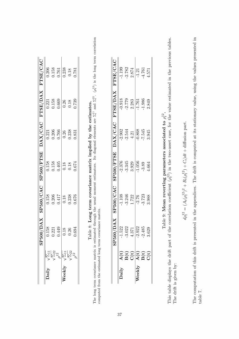
SP
500/
DA
XS
P50
0/C
AC
SP
500/
FT
SE
DA
X/C
AC
FT
SE
/DA
XF
TS
E/C
AC
Dai
ly√
Σ11
0.15
80.
158
0.15
80.
221
0.22
10.
206
√Σ
22
0.22
10.
206
0.15
80.
206
0.15
80.
158
ρ12
0.44
90.
417
0.40
50.
766
0.66
90.
761
Wee
kly
√Σ
11
0.18
0.18
0.18
0.26
0.26
0.23
8√
Σ22
0.26
0.23
80.
180.
238
0.18
0.18
ρ12
0.69
40.
676
0.67
40.
831
0.73
90.
781
Tab
le8:
Lon
gte
rmco
vari
ance
mat
rix
imp
lied
by
the
esti
mat
es.
The
long
term
cova
riance
matr
ixis
esti
mate
dth
rough
the
usu
al
mom
ent
esti
mato
rs.
Its
dia
gonal
elem
ents
are
Σ11t
and
Σ22t
.(ρ
12t
)is
the
long
term
corr
elati
on
com
pute
dfr
om
the
esti
mate
dlo
ng
term
cova
riance
matr
ix.
SP
500/
DA
XS
P50
0/C
AC
SP
500/
FT
SE
DA
X/C
AC
FT
SE
/DA
XF
TS
E/C
AC
Dai
lyA
(t)
-1.5
22-1
.108
-2.3
76-2
.902
-0.9
18-1
.199
B(t
)-3
.022
-3.2
46-3
.345
-2.5
44-2
.779
-2.7
82C
(t)
4.37
11.
722
3.92
94.
212.
283
2.87
4W
eekly
A(t
)-2
.922
-2.7
6-1
.056
-0.8
68-1
.761
-1.2
1B
(t)
-2.4
85-3
.723
-3.8
9-7
.545
-1.9
86-4
.761
C(t
)3.
629
3.98
84.
664
3.94
52.
849
4.57
1
Tab
le9:
Mea
nre
vert
ing
par
amet
ers
asso
ciat
edto
ρ12t
.T
his
tabl
edi
spla
ysth
edr
iftpa
rtof
the
corr
elat
ion
coeffi
cien
t(ρ
12t
)in
the
two-
asse
tca
se,
for
the
valu
ees
tim
ated
inth
epr
evio
usta
bles
.T
hedr
iftis
give
nby
:
dρ
12t
=(A
t(ρ
12t
)2+Bt(ρ
12t
)+Ct)dt
+di
ffusi
onpa
rt.
The
com
puta
tion
ofth
isdr
iftis
pres
ente
din
the
appe
ndic
es.
The
drift
isco
mpu
ted
atit
sst
atio
nary
valu
e,us
ing
the
valu
espr
esen
ted
inta
ble
7.
37
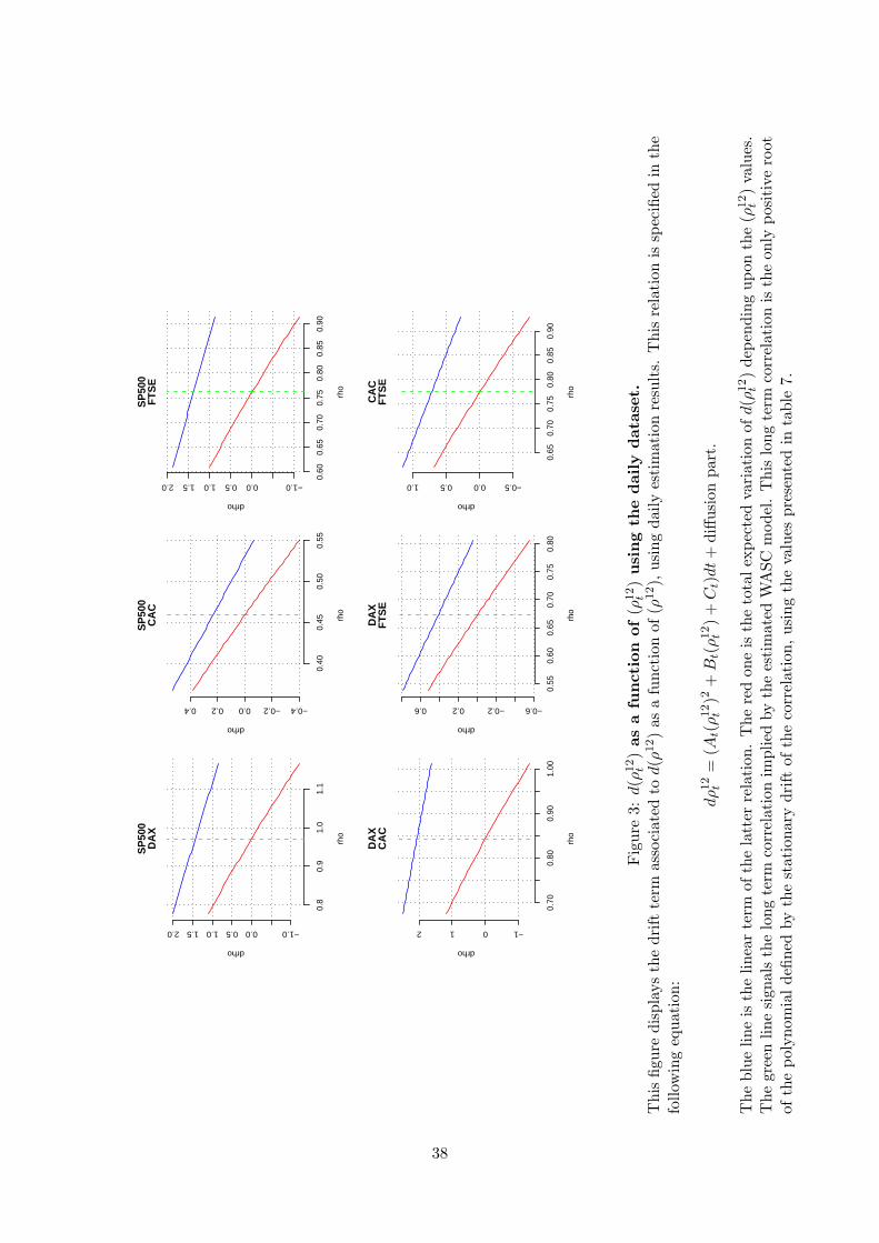
0.8
0.9
1.0
1.1
−1.00.00.51.01.52.0
SP
500
DA
X
rho
drho
0.40
0.45
0.50
0.55
−0.4−0.20.00.20.4
SP
500
CA
C
rho
drho
0.60
0.65
0.70
0.75
0.80
0.85
0.90
−1.00.00.51.01.52.0
SP
500
FTS
E
rho
drho
0.70
0.80
0.90
1.00
−1012
DA
XC
AC
rho
drho
0.55
0.60
0.65
0.70
0.75
0.80
−0.6−0.20.20.6
DA
XFT
SE
rho
drho
0.65
0.70
0.75
0.80
0.85
0.90
−0.50.00.51.0
CA
CFT
SE
rho
drho
Fig
ure
3:d(ρ
12t
)as
afu
nct
ion
of(ρ
12t
)u
sin
gth
ed
aily
dat
aset
.T
his
figur
edi
spla
ysth
edr
iftte
rmas
soci
ated
tod(ρ
12)
asa
func
tion
of(ρ
12),
usin
gda
ilyes
tim
atio
nre
sult
s.T
his
rela
tion
issp
ecifi
edin
the
follo
win
geq
uati
on:
dρ
12t
=(A
t(ρ
12t
)2+Bt(ρ
12t
)+Ct)dt
+di
ffusi
onpa
rt.
The
blue
line
isth
elin
ear
term
ofth
ela
tter
rela
tion
.T
here
don
eis
the
tota
lexp
ecte
dva
riat
ion
ofd(ρ
12t
)de
pend
ing
upon
the
(ρ12t
)va
lues
.T
hegr
een
line
sign
als
the
long
term
corr
elat
ion
impl
ied
byth
ees
tim
ated
WA
SCm
odel
.T
his
long
term
corr
elat
ion
isth
eon
lypo
siti
vero
otof
the
poly
nom
ial
defin
edby
the
stat
iona
rydr
iftof
the
corr
elat
ion,
usin
gth
eva
lues
pres
ente
din
tabl
e7.
38
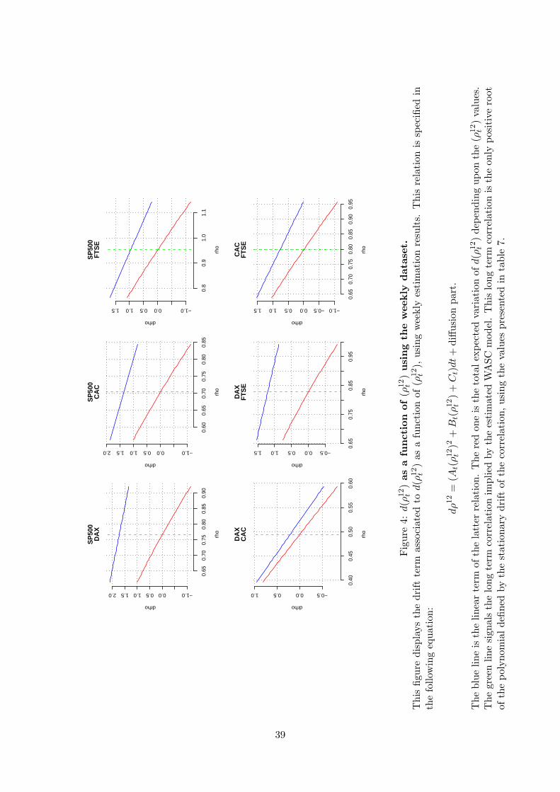
0.65
0.70
0.75
0.80
0.85
0.90
−1.00.00.51.01.52.0
SP
500
DA
X
rho
drho
0.60
0.65
0.70
0.75
0.80
0.85
−1.00.00.51.01.52.0
SP
500
CA
C
rho
drho
0.8
0.9
1.0
1.1
−1.00.00.51.01.5
SP
500
FTS
E
rho
drho
0.40
0.45
0.50
0.55
0.60
−0.50.00.51.0
DA
XC
AC
rho
drho
0.65
0.75
0.85
0.95
−0.50.00.51.01.5
DA
XFT
SE
rho
drho
0.65
0.70
0.75
0.80
0.85
0.90
0.95
−1.0−0.50.00.51.01.5
CA
CFT
SE
rho
drho
Fig
ure
4:d(ρ
12t
)as
afu
nct
ion
of(ρ
12t
)u
sin
gth
ew
eekly
dat
aset
.T
his
figur
edi
spla
ysth
edr
iftte
rmas
soci
ated
tod(ρ
12t
)as
afu
ncti
onof
(ρ12t
),us
ing
wee
kly
esti
mat
ion
resu
lts.
Thi
sre
lati
onis
spec
ified
inth
efo
llow
ing
equa
tion
:
dρ
12
=(A
t(ρ
12t
)2+Bt(ρ
12t
)+Ct)dt
+di
ffusi
onpa
rt.
The
blue
line
isth
elin
ear
term
ofth
ela
tter
rela
tion
.T
here
don
eis
the
tota
lexp
ecte
dva
riat
ion
ofd(ρ
12t
)de
pend
ing
upon
the
(ρ12t
)va
lues
.T
hegr
een
line
sign
als
the
long
term
corr
elat
ion
impl
ied
byth
ees
tim
ated
WA
SCm
odel
.T
his
long
term
corr
elat
ion
isth
eon
lypo
siti
vero
otof
the
poly
nom
ial
defin
edby
the
stat
iona
rydr
iftof
the
corr
elat
ion,
usin
gth
eva
lues
pres
ente
din
tabl
e7.
39
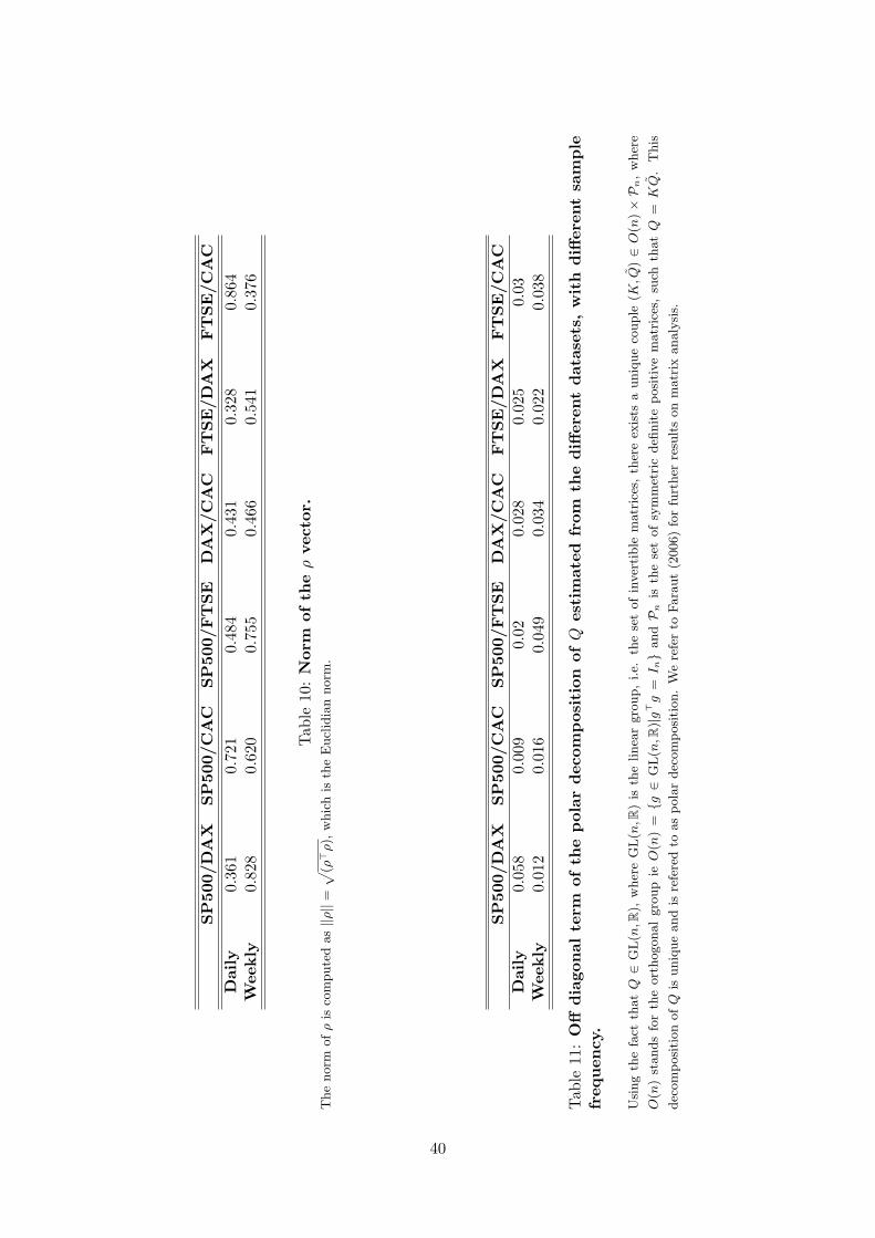
SP
500/
DA
XS
P50
0/C
AC
SP
500/
FT
SE
DA
X/C
AC
FT
SE
/DA
XF
TS
E/C
AC
Dai
ly0.
361
0.72
10.
484
0.43
10.
328
0.86
4W
eekly
0.82
80.
620
0.75
50.
466
0.54
10.
376
Tab
le10
:N
orm
ofth
eρ
vect
or.
The
norm
ofρ
isco
mpute
das||ρ||
=√ (ρ
>ρ),
whic
his
the
Eucl
idia
nnorm
.
SP
500/
DA
XS
P50
0/C
AC
SP
500/
FT
SE
DA
X/C
AC
FT
SE
/DA
XF
TS
E/C
AC
Dai
ly0.
058
0.00
90.
020.
028
0.02
50.
03W
eekly
0.01
20.
016
0.04
90.
034
0.02
20.
038
Tab
le11
:O
ffd
iago
nal
term
ofth
ep
olar
dec
omp
osit
ion
ofQ
esti
mat
edfr
omth
ed
iffer
ent
dat
aset
s,w
ith
diff
eren
tsa
mp
lefr
equ
ency
.
Usi
ng
the
fact
thatQ∈
GL
(n,R
),w
her
eG
L(n,R
)is
the
linea
rgro
up,
i.e.
the
set
of
inver
tible
matr
ices
,th
ere
exis
tsa
uniq
ue
couple
(K,Q
)∈O
(n)×Pn,
wher
e
O(n
)st
ands
for
the
ort
hogonal
gro
up
ieO
(n)
=g∈
GL
(n,R
)|g>g
=I n
andPn
isth
ese
tof
sym
met
ric
defi
nit
ep
osi
tive
matr
ices
,su
chth
atQ
=KQ
.T
his
dec
om
posi
tion
ofQ
isuniq
ue
and
isre
fere
dto
as
pola
rdec
om
posi
tion.
We
refe
rto
Fara
ut
(2006)
for
furt
her
resu
lts
on
matr
ixanaly
sis.
40
Related Documents