Estimating the spatiotemporal distribution of geochemical parameters associated with biostimulation using spectral induced polarization data and hierarchical Bayesian models

Estimating the spatiotemporal distribution of geochemicalparameters associated with biostimulation using spectralinduced polarization data and hierarchical Bayesian models

Jinsong Chen,1 Susan S. Hubbard,1 Kenneth H. Williams,1 Adrian Flores Orozco,2

and Andreas Kemna2

Received 1 June 2011; revised 26 March 2012; accepted 17 April 2012; published 30 May 2012.

[1] We developed a hierarchical Bayesian model to estimate the spatiotemporaldistribution of aqueous geochemical parameters associated with in-situ bioremediationusing surface spectral induced polarization (SIP) data and borehole geochemicalmeasurements collected during a bioremediation experiment at a uranium-contaminatedsite near Rifle, Colorado (USA). The SIP data were first inverted for Cole-Cole parameters,including chargeability, time constant, resistivity at the DC frequency, and dependencefactor, at each pixel of two-dimensional grids using a previously developed stochasticmethod. Correlations between the inverted Cole-Cole parameters and the wellbore-basedgroundwater chemistry measurements indicative of key metabolic processes within theaquifer (e.g., ferrous iron, sulfate, uranium) were established and used as a basis forpetrophysical model development. The developed Bayesian model consists of three levelsof statistical submodels: (1) data model, providing links between geochemical andgeophysical attributes, (2) process model, describing the spatial and temporal variability ofgeochemical properties in the subsurface system, and (3) parameter model, describing priordistributions of various parameters and initial conditions. The unknown parameters wereestimated using Markov chain Monte Carlo methods. By combining the temporallydistributed geochemical data with the spatially distributed geophysical data, we obtained thespatiotemporal distribution of ferrous iron, sulfate, and sulfide, and their associateduncertainty information. The obtained results can be used to assess the efficacy of thebioremediation treatment over space and time and to constrain reactive transport models.

Citation: Chen, J., S. S. Hubbard, K. H. Williams, A. Flores Orozco, and A. Kemna (2012), Estimating the spatiotemporal distribution

of geochemical parameters associated with biostimulation using spectral induced polarization data and hierarchical Bayesian models,

Water Resour. Res., 48, W05555, doi:10.1029/2011WR010992.

1. Introduction[2] In-situ bioremediation is often considered as a key

approach for subsurface environmental remediation, andeffective monitoring and understanding of biogeochemicalprocesses are critical for success of the treatment [Andersonet al., 2003; Vrionis et al., 2005; Yabusaki et al., 2007].Geophysical methods, especially spectral induced polariza-tion (SIP), have been shown to be very useful for providingremote information about bioremediation processes. This isbecause the accumulation of mineral precipitates, reactiveions, and biomass that are induced through the bioremedia-tion process may collectively affect the electrical response

[Ntarlagiannis et al., 2005]. Although it has been recognizedthat SIP methods can be used to characterize and identifycontaminants at the field scale [Olhoeft, 1992; Vanhala,1997; Sogade et al., 2006], the value of SIP methods formonitoring remediation-induced solid phase end-productshas mostly been demonstrated through laboratory experi-ments. For example, Williams et al. [2005] established thatSIP responses track the onset and space-time distribution ofbioremediation-induced FeS precipitates using laboratorycolumn experimental data. Slater et al. [2007] showed theSIP signatures are diagnostic of porescale geometricalchanges associated with FeS bioremediation by sulfate reduc-ing bacteria. Personna et al. [2008] used laboratory columnexperimental data to track the onset of anaerobic conditionsand the reoxidation to aerobic conditions through SIP’s sensi-tivity to iron sulfide precipitation and dissolution. Chen et al.[2009] developed a state-space Bayesian model that allowedquantitative estimation of the evolution of bioremediation-induced FeS precipitates and associated permeability reduc-tion using time-lapse SIP data collected in a laboratorycolumn experiment.

[3] However, monitoring the evolution of solid-phaseend-products is not a standard approach for evaluating the

1Earth Sciences Division, Lawrence Berkeley National Laboratory,Berkeley, California, USA.

2Department of Geodynamics and Geophysics, University of Bonn,Bonn, Germany.

Corresponding author: J. Chen, Earth Sciences Division, LawrenceBerkeley National Laboratory, 1 Cyclotron Rd., MS 90-1116, Berkeley, CA94720, USA. ([email protected])

This paper is not subject to U.S. copyright.Published in 2012 by the American Geophysical Union

W05555 1 of 25

WATER RESOURCES RESEARCH, VOL. 48, W05555, doi:10.1029/2011WR010992, 2012

efficacy of bioremediation at the field scale. Instead, theonset and extent of bioremediation is typically inferred bymeans of monitoring changes in geochemical parametersfrom groundwater samples, such as electron acceptor con-sumption, various final products (e.g., dissolved iron or sul-fides), and concentrations of dissolved hydrogen based onaqueous wellbore measurements [e.g., Lovley et al., 1994].The geochemical measurements are also often used toinvestigate the underlying biogeochemical processes at theborehole sampling locations and to constrain reactive trans-port models [e.g., Li et al., 2010].

[4] Several recent studies have qualitatively illustratedthe potential of SIP imaging for tracking subsurface geo-chemical changes associated with bioremediation at thefield scale. Williams et al. [2009, 2011] showed that thephase response in SIP images was associated with changesin groundwater geochemistry accompanying stimulatediron and sulfate reduction and sulfide mineral precipitation.Commer et al. [2011] performed a three-dimensional (3-D)inversion of time-lapse surface SIP data collected during abioremediation and documented the change in phase andresistivity associated with the treatment. Johnson et al.[2010] developed a parallel distributed-memory forwardand inverse modeling algorithm for analyzing resistivityand time domain induced-polarization (IP) data and appliedit to the Brandywine field site in Maryland for monitoringbioremediation. Flores Orozco et al. [2011] reported agood correlation between the increase in the SIP phaseresponse and the increases in Fe(II) and precipitation ofmetal sulfides following biostimulation, reflecting preserva-tion of geochemically reduced conditions within the aqui-fer, for the SIP measurements collected over two years ofmonitoring and for different experiments.

[5] Our goal in this study is to provide quantitative infor-mation on the spatiotemporal distribution of remediation-induced changes in aqueous chemical species that areindicative of redox status (i.e., ferrous iron or Fe2, sulfateand sulfide) through integrating 2-D SIP data with sparsewellbore aqueous geochemical measurements. The primarychallenge of the estimation is to handle properly the dis-crepancy between the temporal sampling frequency and thespatial resolution of the different types of measurements.We can measure aqueous geochemical concentrations overtime (dense in time) as done at the laboratory during biore-mediation treatments. Because drilling boreholes is inva-sive and costly, we can only sample them at very smallnumbers of locations (sparse in space). Surface SIP datahave a large spatial coverage (tens of meters) ; hence, themeasurement support scale is much larger than that associ-ated with a typical wellbore sample. However, surface SIPdata typically have lower spatial resolution relative to thewellbore geochemical measurements.

[6] In this study we develop a hierarchical Bayesianmodel based on time-lapse surface SIP and wellbore geo-chemical data collected at the Department of Energy(DOE) Integrated Field Research Challenge (IFRC) Sitenear Rifle, Colorado to estimate the spatiotemporal distri-bution of aqueous geochemical parameters associated witha subsurface biostimulation experiment. We combine theborehole geochemical measurements, having high temporalresolution but being spatially sparse, with the surface SIPdata, having large coverage but low temporal resolution,

within the Bayesian framework. We use Markov chainMonte Carlo (MCMC) sampling methods to explore thejoint posterior probability distribution.

[7] The remainder of this paper is organized as follows.Section 2 describes the Rifle site and results of data analy-sis, which provide basis for development of the hierarchicalBayesian model. Section 3 describes the hierarchicalBayesian framework and the MCMC sampling approachfor estimating the spatiotemporal distribution using bore-hole geochemical time series and SIP data. The estimationresults are given in section 4 and discussion and conclu-sions are provided in sections 5.

2. Geophysical and Geochemical Measurementsand Data Analysis2.1. In-Situ Bioremediation

[8] Numerous in-situ bioremediation experiments havebeen carried out at the DOE IFRC Rifle site from 2002 to2009 [Williams et al., 2011]. The experiments have beenconducted within an unconfined fluvial aquifer thatincludes sandy gravely unconsolidated sediments with vari-able clay content and that is underlain (at 5.9–7.0 m belowthe ground surface) by a relatively impermeable, regionalaquitard known as the Wasatch formation [Williams et al.,2011], which consists of the variegated mudstones and con-glomeratic sandstones [Lorenz, 1982]. X-ray diffraction(XRD) analysis of the clay-sized fraction (<2 mm) of Riflealluvium identified the primary clay minerals to be smec-tite, illite, and kaolinite, with smectites most abundant(K. H. Williams, unpublished data, 2011). The water tableis located around 3.5 m below the ground surface, with fluc-tuations (less than 1 m) along the year. At the Rifle site,IFRC investigators have repeatedly demonstrated the abilityto remove uranium rapidly from the tailings-contaminatedgroundwater by stimulating the activity of iron- and sulfate-reducing bacteria through acetate amendment [e.g., Andersonet al., 2003; Vrionis et al., 2005; Williams et al., 2011].

[9] The transition from iron reduction to sulfate reduc-tion at the Rifle site occurs at relatively predictable timesfollowing the amendment injection [Yabusaki et al., 2007;Li et al., 2010]. Injection of acetate (electron donor) isinitially going to stimulate the activity of iron-reducingbacteria (Geobacter) commonly found in Rifle sediments[Williams et al., 2011]. Iron reduction is expected to reduceiron (hydro-) oxide to ferrous iron Fe(II) or Fe2, simultane-ously with aqueous U(VI) to immobile U(IV). After thedepletion of ‘‘bioavailable’’ iron, sulfate is expected to bereduced by sulfate reducers (sulfate reducing proteobacte-ria), which should lead to the accumulation of aqueousS(-II) and eventually the formation of amorphous FeS(am).

[10] Our study focuses on a 36-days acetate injectionexperiment from 22 July 2009 to 27 August 2009 (seeFigure 1). During the field experiment, the site groundwaterwas amended with sodium acetate, with target concentra-tions of 15 mM, and sodium bromide, with target concen-trations of 1.3 mM. The acetate and bromide amendedgroundwater were injected to the aquifer via ten boreholes(G51–G60). Groundwater samples were collected through-out the experiment from three up gradient monitoringwells (U01–U03) and 12 down gradient monitoring wells(D01–D12).

W05555 CHEN ET AL.: ESTIMATING GEOCHEMICAL PARAMETERS USING SIP DATA W05555

2 of 25

2.2. Surface SIP Data and Cole-Cole ParameterEstimation

[11] To monitor and understand the in-situ bioremedia-tion processes, surface spectral induced polarization (SIP)data were collected along array A by using a ZongeGDP32(II) with 15 channels on three days, i.e., 22 July2009 (before injection), 10 August 2009 (during injection),and 29 August 2009 (after injection). The measurementswere made by deploying 30 Cu/CuSO4 nonpolarizing elec-trodes (�4 cm in radius) with a separation of 1 m betweenelectrodes. We used coaxial cables to connect the electro-des with the receivers to reduce electromagnetic couplingeffects, as demonstrated by Flores Orozco et al. (Time-lapse spectral induced polarization imaging of stimulateduranium bioremediation, submitted to Near Surface Geo-phys.). The measurement frequencies were selected basedon the equipment constraints (i.e., 0.0625, 0.125, 0.25, 0.5,1, 2, 4, 8, 16, 32, 64, 128, and 256 Hz). We repeated themeasurements twice for frequencies below 2 Hz andrepeated 4, 8, 16, 32, 64, 128, 256 times for higher frequen-cies (increasing by power of two with the increasing of theacquisition frequencies). We measured contact resistancesbefore every survey and found a good contact between theelectrodes and the ground, with values of �700 V. Weinjected electric currents between the electrodes with a con-stant voltage of 55 V, which results in current densities of�150 mA.

[12] The phase and amplitude estimates were obtainedfrom the recorded data using the least-squares based inver-sion method developed by Kemna [2000] and detailed proc-essing for the Rifle data were given by Flores Orozco et al.[2011]. Figure 2 shows the phases in milliradians (mrad) asa function of frequencies on 10 August 2009 along thecross section from depth z ¼ 0 m to z ¼ 10 m and horizon-tal distance from x ¼ 0 m to x ¼ 30 m, with grid sizes of

dx ¼ dz ¼ 0.5 m. The domain that we focus on in this studynearly traverses the sampling boreholes D1, D2, D3, andD4 (see Figure 1). We can see that the spatial distributionof the phase changes over frequencies between 0.0625 and32 Hz and almost no change is observed for frequenciesbeyond 32 Hz. As observed in previous studies performed atthe site [Williams et al., 2009; Flores Orozco et al., 2011],for the frequency range analyzed in our study (<32 Hz), thepolarization response at the Rifle site during biostimulationis mainly controlled by charge transfer processes takingplace at the interface between pore water and the surface ofthe precipitated semiconductive (metallic) minerals.

[13] We use the obtained amplitude and phase valuesand a stochastic inversion method developed by Chen et al.[2008] to estimate Cole-Cole parameters, such as DC resis-tivity, chargeability, time constant, and dependence factor.Since the inclusion of amplitude data makes the fitting ofthe phase data significantly worse, we use only the phasedata in this study. Figure 3 shows the data misfits of thephase data at the four nearby boreholes (i.e., D1, D2, D3,and D4) on the three survey days (i.e., 22 July, 10 August,and 29 August) using a simple or double Cole-Cole model,depending on data sets. Even in this case where we onlyhave measurements at ten different frequencies, these fig-ures show that the fitted curves generally follow the phasedata well. For some data sets, we can see two peaks, whichmay suggest a better fitting by the superposition of a doubleCole-Cole model as done by Cosenza et al. [2007]. Figure 4shows the histograms of root-mean-squares (RMS) ofthe differences between the measured and calculated phaseresponses for 5000 random samples. We generally havesmaller misfits for those data collected at borehole D1 andon 10 August 2009 (during injection).

[14] We can similarly fit the SIP data at other pixels ofthe 20� 20 grids to get Cole-Cole model parameters along

Figure 1. Schematic plan view of the 2009 bioremediation experiment. The open circles (G51–G60)are the ten injection boreholes and the solid circles (D01–D12) are the 12 down gradient monitoringwells. The open triangles (U01–U03) are the three up gradient monitoring wells and the dashed line isthe survey profile of surface spectral induced polarization (SIP) used for this study.

W05555 CHEN ET AL.: ESTIMATING GEOCHEMICAL PARAMETERS USING SIP DATA W05555

3 of 25

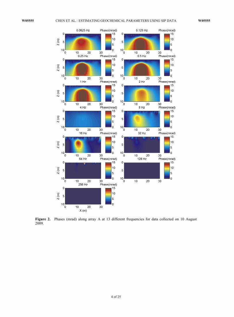
Figure 2. Phases (mrad) along array A at 13 different frequencies for data collected on 10 August2009.

W05555 CHEN ET AL.: ESTIMATING GEOCHEMICAL PARAMETERS USING SIP DATA W05555

4 of 25

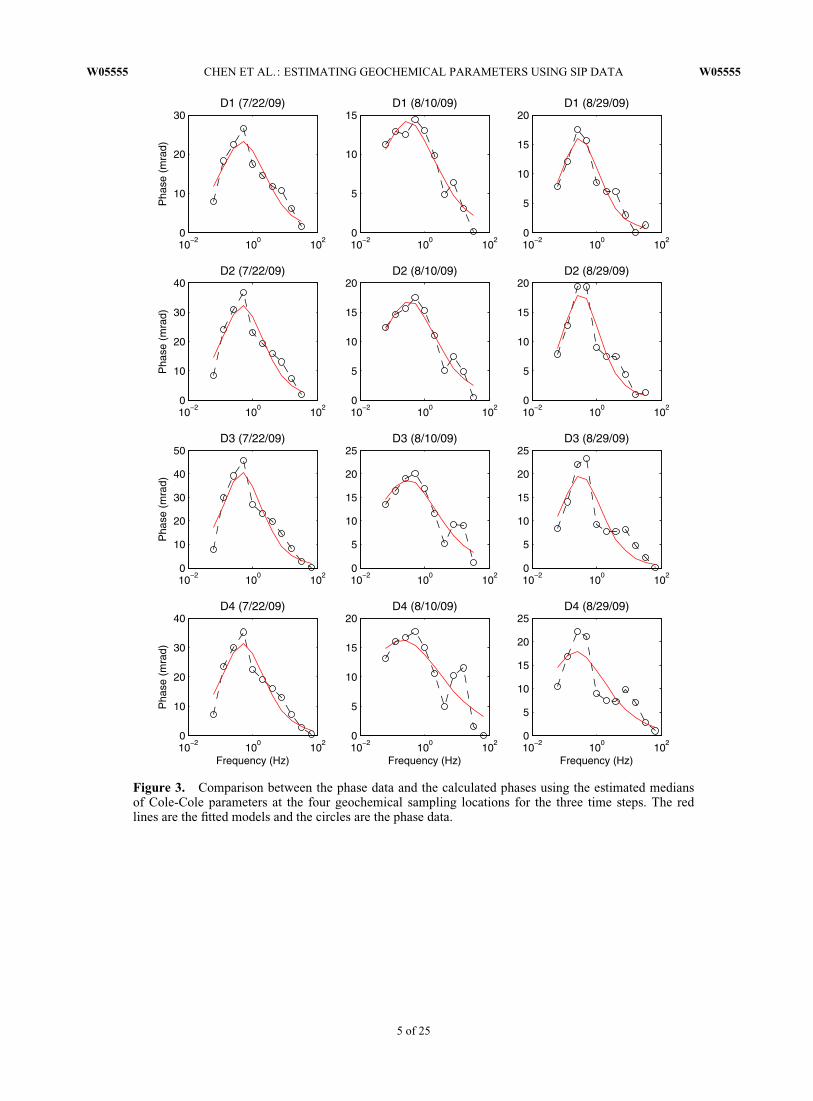
Figure 3. Comparison between the phase data and the calculated phases using the estimated mediansof Cole-Cole parameters at the four geochemical sampling locations for the three time steps. The redlines are the fitted models and the circles are the phase data.

W05555 CHEN ET AL.: ESTIMATING GEOCHEMICAL PARAMETERS USING SIP DATA W05555

5 of 25

Figure 4. Histograms of the root-mean-squares (RMS) of the differences between the measured andcalculated phases for 5000 random samples after Markov chains are converged.

W05555 CHEN ET AL.: ESTIMATING GEOCHEMICAL PARAMETERS USING SIP DATA W05555

6 of 25

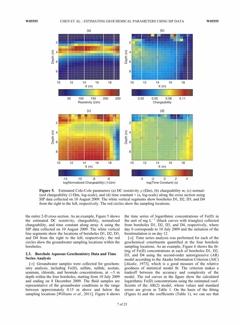
the entire 2-D cross section. As an example, Figure 5 showsthe estimated DC resistivity, chargeability, normalizedchargeability, and time constant along array A using theSIP data collected on 10 August 2009. The white verticalline segments show the locations of boreholes D1, D2, D3,and D4 from the right to the left, respectively; the redcircles show the groundwater sampling locations within theboreholes.

2.3. Borehole Aqueous Geochemistry Data and TimeSeries Analysis

[15] Groundwater samples were collected for geochem-istry analysis, including Fe(II), sulfate, sulfide, acetate,uranium, chloride, and bromide concentrations, at �5 mdepth within the four boreholes, starting from 10 July 2009and ending on 8 December 2009. The fluid samples arerepresentative of the groundwater conditions in the rangebetween approximately 0.15 m above and below thesampling locations [Williams et al., 2011]. Figure 6 shows

the time series of logarithmic concentrations of Fe(II) inthe unit of mg L�1 (black curves with triangles) collectedfrom boreholes D1, D2, D3, and D4, respectively, whereday 0 corresponds to 10 July 2009 and the initiation of thebiostimulation is on day 12.

[16] Time series analysis was performed for each of thegeochemical constituents quantified at the four boreholesampling locations. As an example, Figure 6 shows the fit-ting of Fe(II) concentrations at each of boreholes D1, D2,D3, and D4 using the second-order autoregressive (AR)model according to the Akaike Information Criterion (AIC)[Akaike, 1973], which is a good measure of the relativegoodness of statistical model fit. The criterion makes atradeoff between the accuracy and complexity of themodel. The red curves in the figure show the calculatedlogarithmic Fe(II) concentrations using the estimated coef-ficients of the AR(2) model, whose values and standarderrors are given in Table 1. On the basis of the fitting(Figure 6) and the coefficients (Table 1), we can see that

Figure 5. Estimated Cole-Cole parameters (a) DC resistivity � (Vm), (b) chargeability m, (c) normal-ized chargeability (1/Vm, log-scale), and (d) time constant � (s, log-scale) along the cross section usingSIP data collected on 10 August 2009. The white vertical segments show boreholes D1, D2, D3, and D4from the right to the left, respectively. The red circles show the sampling locations.

W05555 CHEN ET AL.: ESTIMATING GEOCHEMICAL PARAMETERS USING SIP DATA W05555

7 of 25

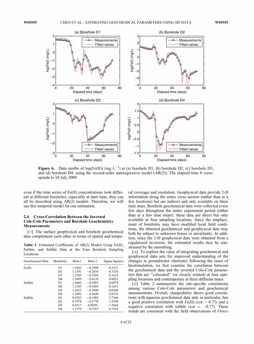
even if the time series of Fe(II) concentrations look differ-ent at different boreholes, especially at later time, they canall be described using AR(2) models. Therefore, we willuse this temporal model for our estimation.

2.4. Cross-Correlation Between the InvertedCole-Cole Parameters and Borehole GeochemistryMeasurements

[17] The surface geophysical and borehole geochemicaldata complement each other in terms of spatial and tempo-

ral coverage and resolution. Geophysical data provide 2-Dinformation along the entire cross section (rather than at afew locations) but are indirect and only available on threetime steps. Borehole geochemical data were collected everyfew days throughout the entire experiment period (ratherthan at a few time steps) ; these data are direct but onlyavailable at four sampling locations. Since the emplace-ment of boreholes may have modified local field condi-tions, the obtained geochemical and geophysical data mayboth be subject to unknown biases or uncertainty. In addi-tion, since the 2-D geophysical data were obtained from aregularized inversion, the estimated results may be con-strained by the smoothing.

[18] To explore the value of integrating geochemical andgeophysical data sets for improved understanding of thechanges in groundwater chemistry following the onset ofbiostimulation, we first examine the correlation betweenthe geochemical data and the inverted Cole-Cole parame-ters that are ‘‘colocated’’ (or closely related) at four sam-pling locations and contemporary at three different times.

[19] Table 2 summarizes the site-specific correlationsamong various Cole-Cole parameters and geochemicalmeasurements. Overall, chargeability shows good correla-tions with aqueous geochemical data and, in particular, hasa good positive correlation with Fe(II) (cor ¼ 0.73) and anegative correlation with sulfide (cor ¼ �0.77). Thesetrends are consistent with the field observations of Flores

Figure 6. Data misfits of log(Fe(II)) (mg L�1) at (a) borehole D1, (b) borehole D2, (c) borehole D3,and (d) borehole D4, using the second-order autoregressive model (AR(2)). The elapsed time 0 corre-sponds to 10 July 2009.

Table 1. Estimated Coefficients of AR(2) Models Using Fe(II),Sulfate, and Sulfide Data at the Four Borehole SamplingLocations

Geochemical Data Boreholes Beta-1 Beta-2 Sigma Squares

Fe(II) D1 1.1842 �0.2900 0.3331D2 1.1391 �0.2434 0.3324D3 1.2385 �0.3584 0.1619D4 1.2499 �0.4126 0.0825

Sulfate D1 1.4402 �0.5987 0.0974D2 1.2345 �0.3485 0.1653D3 1.3653 �0.5900 0.0340D4 1.2496 �0.5649 0.0518

Sulfide D1 0.9282 �0.1903 2.7106D2 0.7978 �0.2778 3.3594D3 0.4517 0.0549 1.3664D4 1.1579 �0.2767 0.7418

W05555 CHEN ET AL.: ESTIMATING GEOCHEMICAL PARAMETERS USING SIP DATA W05555

8 of 25

Orozco et al. [2011] and the laboratory studies of Williamset al. [2009]. Although we have only a total number of 12data points for the analysis, the consistence with otherstudies gives us confidence to apply a linear relationship tolink Cole-Cole parameters to geochemical data in the laterstudy.

3. Hierarchical Spatiotemporal Bayesian Model[20] We develop a Bayesian model based on the results

of data analysis presented in section 2 to estimate the spatio-temporal distributions of Fe(II), sulfate, and sulfide concen-trations using the chargeability data, as those geochemicalparameters are important indicators of the status of the bio-remediation treatment. Although the chargeability data maybe linked to those geochemical parameters as a multivariatevariable, in this study we choose to estimate each of thegeochemical parameters separately from the chargeabilitydata because we cannot derive a reliable multivariate rela-tionship between chargeability and geochemical data giventhe limited colocated and contemporary data points.

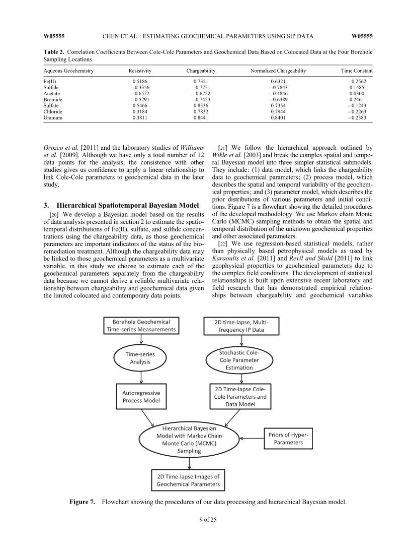
[21] We follow the hierarchical approach outlined byWikle et al. [2003] and break the complex spatial and tempo-ral Bayesian model into three simpler statistical submodels.They include: (1) data model, which links the chargeabilitydata to geochemical parameters; (2) process model, whichdescribes the spatial and temporal variability of the geochem-ical properties; and (3) parameter model, which describes theprior distributions of various parameters and initial condi-tions. Figure 7 is a flowchart showing the detailed proceduresof the developed methodology. We use Markov chain MonteCarlo (MCMC) sampling methods to obtain the spatial andtemporal distribution of the unknown geochemical propertiesand other associated parameters.

[22] We use regression-based statistical models, ratherthan physically based petrophysical models as used byKaraoulis et al. [2011] and Revil and Skold [2011] to linkgeophysical properties to geochemical parameters due tothe complex field conditions. The development of statisticalrelationships is built upon extensive recent laboratory andfield research that has demonstrated empirical relation-ships between chargeability and geochemical variables

Table 2. Correlation Coefficients Between Cole-Cole Parameters and Geochemical Data Based on Colocated Data at the Four BoreholeSampling Locations

Aqueous Geochemistry Resistivity Chargeability Normalized Chargeability Time Constant

Fe(II) 0.5186 0.7321 0.6321 �0.2562Sulfide �0.3356 �0.7751 �0.7843 0.1485Acetate �0.6522 �0.6722 �0.4846 0.0300Bromide �0.5291 �0.7423 �0.6389 0.2461Sulfate 0.5466 0.8336 0.7354 �0.1243Chloride 0.3184 0.7832 0.7944 �0.2263Uranium 0.3811 0.8441 0.8401 �0.2383

Figure 7. Flowchart showing the procedures of our data processing and hierarchical Bayesian model.

W05555 CHEN ET AL.: ESTIMATING GEOCHEMICAL PARAMETERS USING SIP DATA W05555

9 of 25

[Ntargialiannis et al., 2005; Slater et al., 2006, 2007;Personna et al., 2008; Williams et al., 2005, 2009, 2011;Chen et al., 2009; Wu et al., 2011; Flores Orozco et al.,2011]. We acknowledge that the use of regression-basedstatistical models is a limitation of the current studybecause they are site specific and may be biased. Findingphysically based petrophysical models is an active area ofresearch in the community, and it is not the focus of this pa-per. However, the developed methodology can be extendedto the cases where physically based models are available.

3.1. Data Model

[23] The data model links the inverted chargeability togeochemical concentrations at each pixel. Although wemay use the correlation coefficients obtained throughregression of the colocated data, we consider them asunknowns for more general cases. Let utðsÞ be the unknownconcentration at grid s 2 D ¼ f1; 2; . . . ;mg, where m isthe total number of sites, and at time step t 2 T ¼f1; 2; . . . ; ng, where n is the total number of time steps. Letmobs

t ðsÞ be the chargeability data, where s 2 D and t 2 Tg,which is a subset of set T and represents the three SIP sur-vey days. From regression analysis of the colocated andcontemporary geochemical and geophysical data, we canassume that there is a linear relationship between the aque-ous geochemical and chargeability data. The linear assump-tion is derived from field data rather than from theory. Atthe early stage of our understanding of the SIP responses togeochemical heterogeneity, we feel more comfortable touse field-derived empirical relationships instead of theoreti-cal relationships for the estimation. Consequently, we havemobs

t ðsÞ ¼ �1 þ �2utðsÞ þ "m, where �1 and �2 areunknown coefficients, and "m is the random error thataccounts for uncertainty from multiple sources, such aserrors in the petrophysical model and in the inverted charge-ability data.

[24] Since the chargeability data were obtained from fit-ting the inverted surface IP data, which typically have aspatially variable resolution, we may allow the coefficients(i.e., �1 and �2) to be varied over the space. However, inthis study, because we only use the data on a small subdo-main, ranging from x ¼ 10 m to x ¼ 20 m and z ¼ 2 m toz ¼ 6 m, on which the coefficients of variation of sensitiv-ity are 1% laterally and 5% vertically, we ignore such var-iations. Therefore, we assume that both coefficients �1 and�2 are same at each pixel and the errors at different loca-tions are independent. We address the spatial variability bythe additive error "m, which is assumed to have a Gaussiandistribution with the inverse variance of �m.

[25] We can describe the data model using vectors forconciseness. Let mobs

t ¼ fmobst ðsÞ; s 2 Dg and ut ¼ futðsÞ;

s 2 Dg. We thus have the following conditional probabilitydistribution for geophysical data:

½fmobst ; t 2 Tggjfut; t 2 Tgg; �1; �2; �m� ¼

Yt2Tg

½mobst jut; �1; �2; �m�;

(1)

where we use the bracket to denote probability distribu-tion in equation (1) following the annotation provided byGelfand and Smith [1990]. We can similarly obtain adata model for borehole geochemical measurements.

However, because the errors in the borehole data are typ-ically much smaller than those in the regression model inequation (1), we consider them as true values at the bore-hole locations in this study. Let uobs

t ðsÞ be the directmeasurements of geochemical concentrations at timet 2 T and site s 2 Db, which is a subset of set D and rep-resents the four borehole sampling locations. We thushave utðsÞ ¼ uobs

t ðsÞ.3.2. Process Model

[26] We use a statistical rather than mechanistic (or re-active transport) model to simulate the evolution of geo-chemical processes. Since we can fit the geochemical timeseries using the second order autoregressive models assuggested by data analysis (see Table 1), we model theevolution processes using the following relationship:utðsÞ ¼ �1ðsÞut�1ðsÞ þ �2ðsÞut�2ðsÞ þ "uðsÞ, where �1ðsÞand �2ðsÞ are the coefficients at site s 2 D. The spatiallyvariable coefficients allow us to take account for the heter-ogeneity of geochemical properties as recognized by Liet al. [2009]. We consider "uðsÞ as a stationary spatial pro-cess, and it has the inverse variance of �pu and the correla-tion matrix determined by the following exponentialvariogram function:

rðsi; sjÞ ¼ exp �

ffiffiffiffiffiffiffiffiffiffiffiffiffiffiffiffiffiffiffiffiffiffiffiffiffiffiffiffiffiffiffiffiffiffiffiffiffiffiffiffiffiffiffiffiffiffiffiffiffiffiffiffiffiffiffiffiffiffiffiffiffiffiffiffiffiffiffiffiffiffiffixðsiÞ � xðsjÞ

�x

� �2

þ zðsiÞ � zðsjÞ�z

� �2s8<

:9=;;

(2)

where ðxðsiÞ; zðsiÞÞ and ðxðsjÞ; zðsjÞÞ are the 2-D coordi-nates of si and sj grids, respectively. Symbols �x and �z

are the spatial correlation lengths along lateral and verti-cal directions. Since we do not have direct information todetermine the spatial correlation lengths at this time, weassume that they have similar spatial structure to the per-meability field. Therefore, we pick �x ¼ 2 m and�z ¼ 0:5 m, derived from the permeability fields ofEnglert et al. [2009] and Li et al. [2010]. Let R ¼frðsi; sjÞ; si; sj 2 Dgm�m be the known correlation matrixand let vector eu ¼ ð"uð1Þ; "uð2Þ; . . . ; "uðmÞÞT . Weassume that eu has the multivariate Gaussian distributionwith zero mean and the inverse covariance matrix of�puR�1, i.e., eu � Nð0; �puR�1Þ.

[27] We can simplify the process model by letting b1 andb2 be the diagonal metrics with �1ðsÞ and �2ðsÞ, s 2 D,being the corresponding diagonal terms. Thus, we haveut ¼ b1ut�1 þ b2ut�2 þ eu. Using the same notation, weassume that the initial geochemical concentrations u1 andu2 have multivariate Gaussian distributions, i.e.,u1 � Nð�u1e; �u1R�1Þ and u2 � Nð�u2e; �u2R�1Þ, wheree ¼ ð1; 1; . . . ; 1ÞTm�1 and �u1, �u2, �u1, and �u2 are hyper-parameters having priors determined by borehole logs. Bycombining the above information, we have a spatial andtemporal process model for geochemical parameters asgiven below:

½fut; t 2 Tgjb1; b2; �pu; �u1; �u1; �u2; �u2�

¼ ½u1j�u1; �u1�½u2j�u2; �u2�Yn

k¼3

½uk juk�1; uk�2; b1;b2; �pu�:(3)

W05555 CHEN ET AL.: ESTIMATING GEOCHEMICAL PARAMETERS USING SIP DATA W05555

10 of 25

[28] By combining the data (equation (1)) and process(equation (3)) models, we obtain the following full jointposterior distribution:

fut; t 2 Tg; �1; �2; �m; b1;b2; �pu; �u1; �u1; �u2; �u2jfmobst ; t 2 Tgg

� �/ fmobs

t ; t 2 Tggjfut; t 2 Tgg; �1; �2; �m

� �u1j�u1; �u1½ � u2j�u2; �u2½ � �

Yn

k¼3

uk juk�1; uk�2; b1;b2; �pu

� �

�1; �2; �m; b1;b2; �pu; �u1; �u1; �u2; �u2

� �:

(4)

3.3. Priors on the Parameters

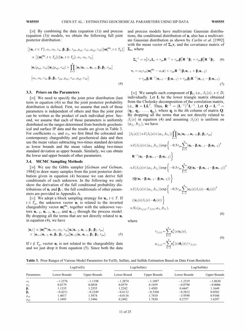
[29] We need to specify the joint prior distribution (lastterm in equation (4)) so that the joint posterior probabilitydistribution is defined. First, we assume that each of thoseparameters is independent of others and thus the joint priorcan be written as the product of each individual prior. Sec-ond, we assume that each of those parameters is uniformlydistributed on the ranges determined from borehole geochem-ical and surface IP data and the results are given in Table 3.For coefficients �1 and �2, we first fitted the colocated andcontemporary chargeability and geochemical data and thenuse the mean values subtracting two-times standard deviationas lower bounds and the mean values adding two-timesstandard deviation as upper bounds. Similarly, we can obtainthe lower and upper bounds of other parameters.

3.4. MCMC Sampling Methods

[30] We use the Gibbs sampler [Gelman and Gelman,1984] to draw many samples from the joint posterior distri-bution given in equation (4) because we can derive fullconditionals of each unknown. In the following we onlyshow the derivation of the full conditional probability dis-tributions of ut and b1 ; the full conditionals of other param-eters are provided in Appendix A.

[31] We adopt a block sampling strategy for ut, t 2 T . Ift 2 Tg, the unknown vector ut is related to the invertedchargeability vector mobs

t , together with the unknown vec-tors ut�2, ut�1, utþ1, and utþ2 through the process model.By dropping all the terms that are not directly related to ut

in equation (4), we have

½utj�� / ½mobst jut; �1; �2; �m�½utjut�2; ut�1; b1; b2; �pu�

� ½utþ1jut�1; ut; b1; b2; �pu�½utþ2jut; utþ1; b1; b2; �pu�: (5)

If t 62 Tg, vector ut is not related to the chargeability dataand we just drop it from equation (5). Since both the data

and process models have multivariate Gaussian distribu-tions, the conditional distribution of ut also has a multivari-ate Gaussian distribution as shown by Carlin et al. [1992]with the mean vector of Ruvt and the covariance matrix ofRu, where

R�1u ¼ �2

2�mIm þ �puR�1 þ �pubT1 R�1b1 þ �pub

T2 R�1b2; (6)

vt ¼ �2�mðmobst � �1eÞ þ �puR�1ðb1ut�1 þ b2ut�2Þ

þ �pub1R�1ðutþ1 � b2ut�1Þ þ �pub2R�1ðutþ2 � b1utþ1Þ:(7)

[32] We sample each component of b1, i.e., �1ðsÞ; s 2 D,individually. Let L be the lower triangle matrix obtainedfrom the Cholesky decomposition of the correlation matrix,i.e., R ¼ LLT . Thus, R�1 ¼ ðL�1ÞT L�1. Let Q ¼ L�1 ¼ðq1; q2; . . . ; qmÞ, where qi is the ith column of matrix Q.By dropping all the terms that are not directly related to�1ðsÞ in equation (4) and assuming �1ðsÞ is uniform onða�1

; b�1Þ, we have

½�1ðsÞj��/Ið�1ðsÞ2ða�1;b�1ÞÞYn

k¼3

½uk juk�1;uk�2;b1;b2;�pu�

/Ið�1ðsÞ2ða�1;b�1ÞÞexp

��0:5�pu

Xn

k¼3

ðuk�b1uk�1�b2uk�2ÞT

R�1ðuk�b1uk�1�b2uk�2Þ�

/Ið�1ðsÞ2ða�1;b�1ÞÞexp

��0:5�pu

Xn

k¼3

ðQðuk�b1uk�1�b2uk�2ÞÞT

ðQðuk�b1uk�1�b2uk�2ÞÞ�

/Ið�1ðsÞ2ða�1;b�1ÞÞexp

��0:5�pu

Xn

k¼3

ðckðsÞ�1ðsÞ�dkðsÞÞT

ððckðsÞ�1ðsÞ�dkðsÞÞ�

/NT ð��1ðsÞ;��1ðsÞ;a�1;b�1Þ;

(8)

where

��1ðsÞ¼Xn

k¼3

cTk ðsÞckðsÞ;

��1ðsÞ¼Xn

k¼3

cTk ðsÞdkðsÞ=��1ðsÞ;

(9)

Table 3. Prior Ranges of Various Model Parameters for Fe(II), Sulfate, and Sulfide Estimation Based on Data From Boreholes

Parameters

Log(Fe(II)) Log(Sulfate) Log(Sulfide)

Lower Bounds Upper Bounds Lower Bound Upper Bounds Lower Bounds Upper Bounds

�1 �1.2376 �1.1198 �1.2874 �1.1897 �1.2319 �1.0630�2 0.0179 0.0838 0.0579 0.1459 �0.0798 �0.0086b1 1.1335 1.2555 1.2242 1.4505 0.4447 1.1649b2 �0.4211 �0.2349 �0.6112 �0.3360 �0.2812 0.0582�u1 1.4017 1.5874 �0.0116 1.7410 �3.9598 0.9106�u2 1.3493 1.5486 0.2482 1.7830 0.2757 1.6297

W05555 CHEN ET AL.: ESTIMATING GEOCHEMICAL PARAMETERS USING SIP DATA W05555

11 of 25

ckðsÞ¼uk�1ðsÞqs;

dkðsÞ¼Xm

i¼1

ðukðiÞ��2ðiÞuk�2ðiÞÞqi�Xm

i6¼s

�1ðiÞuk�1ðiÞqi;(10)

and IðÞ is the indicator function with the value of 1 if thecondition is satisfied and 0 otherwise. The symbol NT rep-resents the truncated normal distribution.

4. Estimation Results[33] We apply the developed Bayesian model and sam-

pling strategy to estimate the spatiotemporal distribution ofFe(II), sulfate, and sulfide concentrations. Since the meth-odology and procedures for estimating different types ofgeochemical parameters are similar, we only show thedetails for Fe(II) estimation but provide results for estima-tion of other parameters.4.1. Priors and Sensitivity of Model Parameters

[34] Since the total number of unknowns is much largerthan the total number of data points, we use informativepriors based on the results of data analysis. We set thelower and upper bounds of �1 and �2 as their correspond-ing regression estimates, minus and plus two-times stand-ard errors. We set the lower and upper bounds of b1, b2, �1,and �2 as the minimum and maximum values obtainedfrom four boreholes with extension by 5% from their origi-nal ranges. Table 3 lists the actual lower and upper boundsused in the study for the Fe(II), sulfate, and sulfideestimation.

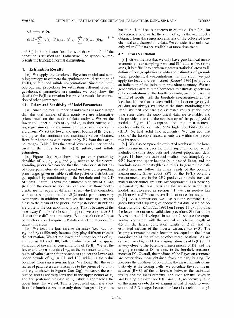
[35] Figures 8(a)–8(d) shows the posterior probabilitydensities of �1, �2, �u1, and �u2, relative to their corre-sponding priors. We can see that the posterior distributionsof those parameters do not depend on their correspondingprior ranges given in Table 3; all the posterior distributionsget updated by conditioning to the borehole and the 2-DSIP data. Figure 9 shows the estimated medians of b1 andb2 along the cross section. We can see that those coeffi-cients are not equal at different sites, which is consistentwith our assumption that the AR(2) model parameters varyover space. In addition, we can see that most medians areclose to the mean of the priors ; their posterior distributionsare close to the corresponding priors. This is because at thesites away from borehole sampling ports we only have SIPdata at three different time steps. Better resolution of thoseparameters would require SIP data collection at more fre-quent time steps.

[36] We treat the four inverse variances (i.e., �u1, �u2,�pu, and �m) differently because they play different roles inthe estimation. We set the lower and upper bounds of �u1

and �u2 as 0.1 and 100, both of which control the spatialvariation of the initial concentrations of Fe(II). We set thelower and upper bounds of �pu as the minimum and maxi-mum of values at the four boreholes and set the lower andupper bounds of �m as 0.l and 100, which is the valueobtained from regression analysis. We found that the esti-mates of parameters are insensitive to the priors of �u1, �u2,and �pu as shown in Figures 8(e)–8(g). However, the esti-mation results are very sensitive to the upper bound of �m

and the posterior estimate of �m always approaches theupper limit that we set. This is because at each site awayfrom the boreholes we have only three chargeability values

but more than three parameters to estimate. Therefore, forthe current study, we fix the value of �m as the one directlyobtained from the regression analysis of the colocated geo-chemical and chargeability data. We consider it as unknownonly when SIP data are available at more time steps.

4.2. Cross Validation

[37] Given the fact that we only have geochemical meas-urements at four sampling ports and SIP data at three timesteps, it is difficult to perform rigorous statistical cross vali-dation of our geophysically obtained estimates of ground-water geochemical concentrations. In this study we justapply the leave-one-out method [Kohavi, 1995] to providean indication of the estimation procedure accuracy. We usegeochemical data at three boreholes to estimate geochemi-cal concentrations at the fourth borehole, and compare theestimated results with the borehole measurements at thatlocation. Notice that at each validation location, geophysi-cal data are always available at the three monitoring timesteps. We first compare the estimated results at the threetime steps when the geophysical data are available, andthis provides a test of the consistency of the petrophysicalmodels. Figure 10 compares the true measurements(circles) with the estimated 95% high probability domain(HPD) (vertical solid line segments). We can see thatmost of the borehole measurements are within the predic-tive intervals.

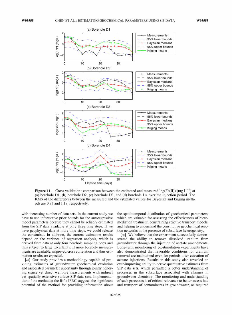
[38] We also compare the estimated results with the bore-hole measurements over the entire injection period, whichincludes the time steps with and without geophysical data.Figure 11 shows the estimated medians (red triangles), the95% lower and upper bounds (blue dashed lines), and theborehole measurements (black circles). In general, the esti-mated medians follow the main trends of the boreholemeasurements. Since about 83% of the Fe(II) boreholemeasurements are in the 95% predictive bounds, our esti-mated uncertainties are little over-optimistic. This possiblyis caused by the small variance that we used in the datamodel. As discussed in section 4.1, we can resolve thisproblem when SIP data are available at more time steps.

[39] As a comparison, we also put the estimates (i.e.,green lines with squares) of geochemical data based on or-dinary kriging [Kitanidis, 1997] on Figure 11 by followingthe leave-one-out cross-validation procedure. Similar to theBayesian model developed in section 2, we use the expo-nential variogram with the vertical correlation length of0.5 m, the lateral correlation length of 2 m, and theestimated median of the inverse variance �u2 (�3). Thekriging estimates at each location are equal to the linearcombination of the values at other three locations. As wecan see from Figure 11, the kriging estimates of Fe(II) at D1is very close to the borehole measurements at D2, and thekriging estimate at D4 is close to the borehole measure-ments at D3. Overall, the medians of the Bayesian estimatesare better than those obtained from ordinary kriging. Tomeasure the goodness of predicting the measurements quan-titatively at the testing wells, we calculate the root-mean-squares (RMS) of the differences between the estimatedresults and the measurements. The RMS for the Bayesianand kriging estimates are 0.83 and 1.18, respectively. Oneof the main drawbacks of kriging is that it leads to over-smoothed 2-D images because the lateral correlation length

W05555 CHEN ET AL.: ESTIMATING GEOCHEMICAL PARAMETERS USING SIP DATA W05555

12 of 25

is 2 m, which is just 1/5 of the horizontal length of the targetdomain. As shown in Figure 12, the kriging estimates yieldan almost spatially uniform distribution of estimated Fe(II)over the 2-D domain.

4.3. Estimated Spatiotemporal Distribution of Fe(II)Concentrations

[40] The developed Bayesian model allows us to esti-mate the spatial distribution of Fe(II) concentrations ateach time step by conditioning to the 2-D geophysical dataand the time series borehole geochemical measurements.Figure 13 shows the medians of Fe(II) concentrations fromday 0 (starting of injection) to day 38 (after injection),obtained using the developed Bayesian procedure and bothgeochemical and geophysical data sets. The 2-D geophysi-cal data are temporally sparse and available only at three timesteps (i.e., day 0, day 20, and day 38), and the geochemical

borehole measurements are spatially sparse and availableonly at four sampling ports showing as circles in Figure 13.The estimated spatiotemporal distribution shows the evolu-tion of Fe(II) concentrations over time during biostimulation.We can see that in the early stage of injection (before day10), the Fe(II) concentrations are approximately uniform onthe cross section. On day 14, the concentrations near theupper-left portion of the imaging region start increasing andbecome most apparent by day 20, a day when 2-D geophysi-cal data are available. Starting on day 30, the Fe(II) concen-trations near the right side of the domain decrease (bluecolors) and at the end of injection, the concentration near thelower right region of the imaging domain is much lower rela-tive to surrounding regions. The estimated results providemore information than the geochemical borehole data alone(i.e., Figure 12) for understanding and monitoring the field-scale bioremediation processes.

Figure 8. Estimated posterior probability densities of hyperparameters.

W05555 CHEN ET AL.: ESTIMATING GEOCHEMICAL PARAMETERS USING SIP DATA W05555

13 of 25

4.4. Estimated Spatiotemporal Distribution of Sulfateand Sulfide Concentrations

[41] To estimate the spatiotemporal distributions of sul-fate and sulfide concentrations, we follow a similar proce-dure as was described for Fe(II). We first fit the geochemicalwellbore time series data using AR(2) models; associatedcoefficients of those fits are also provided in Table 1. Wecan see that the variations in the AR(2) models of boreholesulfate measurements are very similar to those of Fe(II).But the variations of borehole sulfide data are significantlylarger than those of Fe(II) and sulfate. The prior bounds forsulfate and sulfide estimation are given in Table 3. Weadditionally note that the spatial variations of initial sulfateand sulfide concentrations are significantly larger than thoseof Fe(II).

[42] Figures 14(a) and 14(b) show the cross validation ofsulfate and sulfide during the time that geophysical data areavailable. We can see that the predictive ranges of sulfateconcentrations are smaller than those of Fe(II) and most ofthe measured sulfate concentrations are near the upper

bounds of the ranges. This may be caused by the large spa-tial variation in the initial sulfate concentrations. For sulfidewe can see that the predictive ranges of sulfide concentra-tions are considerably larger than those of Fe(II) and sulfateand that the Bayesian model underestimates sulfide valuesfor large concentrations. This is possibly caused by the largevariance in fitting AR(2) models as shown in Table 1.

[43] Figures 15 and 16 show the cross validation for sul-fate and sulfide, respectively, over the entire injection pe-riod. Again, the estimated medians of sulfate and sulfidefollow the main trends of the measurements and slightlybetter than the results of kriging. For sulfide, the Bayesianestimates are considerably smaller than their correspondingborehole measurements.

[44] Figures 17 and 18 show the spatiotemporal distribu-tions of sulfate and sulfide concentrations along the 2-D crosssection, obtained using the developed Bayesian approachthat honors both geochemical and geophysical data sets. Ingeneral, the spatial and temporal patterns of sulfate concen-trations are similar to those of the Fe(II) concentrations, but

Figure 9. Estimated medians of the process model coefficients along the 2-D cross section: (a) �1 and(b) �2.

W05555 CHEN ET AL.: ESTIMATING GEOCHEMICAL PARAMETERS USING SIP DATA W05555

14 of 25

the patterns of sulfide concentrations are opposite. Suchan effect is expected, given that sulfate and sulfide—the met-abolic by-product of sulfate reduction—are negatively corre-lated. Similarly, in locations where Fe(II) is in excess (e.g.,upper left of Figure 13, images from days 16–38), thresholdconcentrations of sulfide will be largely removed from solu-tion, as observed at similar locations in Figure 18. The fig-ures reveal very detailed information about the spatial andtemporal evolution of the geochemical groundwater species.

5. Discussion and Conclusions[45] We have developed a hierarchical Bayesian model

for estimating the spatiotemporal distribution of Fe(II), sul-fate, and sulfide by integrating 2-D geophysical data and‘‘point’’ geochemical borehole measurements. Geophysicaldata have large spatial coverage but are available only at afew time steps, whereas the borehole time series of aqueousgeochemistry data are temporally dense but are availableonly at a few locations. We have shown that integration ofthe geophysical and geochemical data using the developedBayesian approach significantly improves the estimates ofthe evolution of groundwater chemistry associated with abioremediation experiment relative to what is availablebased on wellbore data alone. The developed Bayesianmodel is very flexible and can be applied to estimate othergeochemical parameters, particularly those having a strongcorrelation with Cole-Cole parameters. The method canalso be extended for use with 3-D SIP data.

[46] We chose to estimate aqueous geochemical concentra-tions of ferrous iron, sulfate, and sulfide because these speciesare commonly used to assess the onset and evolution of biore-mediation treatments. This work advances previous estimationstudies, where we focused on using SIP data to estimate theevolution of remediation induced solid phase end-products(such as FeS) and their impact on hydraulic parameters.

[47] The cross validation using the leave-one-out methodshows that the majority of true measurements are within the95% predictive intervals and the estimated medians approx-imately follow the main treads of the corresponding truevalues. But the point-to-point comparison of the estimatedand measured time series is not impressive. Especially forsulfide estimation, the estimated results are substantiallysmaller than the corresponding borehole measurements. Thespatial sparseness of the geochemical data and temporalsparseness of the geophysical data are interpreted to be themain culprits for this unsatisfactory comparison. However,the benefit of incorporating geophysical data in the estimationof geochemical parameters was substantial, as was illustratedthrough comparison of the Bayesian estimates (Figure 13)with kriging wellbore (Figure 12) estimates, the latter ofwhich were almost spatially uniform and provided little infor-mation about the evolution of the groundwater chemistry fol-lowing biostimulation.

[48] We made several key assumptions on the priors anderror structures in the current Bayesian model based on thecurrent available data sets and some may become less critical

Figure 10. Cross validation: comparison between the estimated and measured log(Fe(II)) at the timestep that SIP data are available. The vertical segments are the estimated 95% highest probability domains(HPD), and the circles are the borehole measurements.

W05555 CHEN ET AL.: ESTIMATING GEOCHEMICAL PARAMETERS USING SIP DATA W05555

15 of 25

with increasing number of data sets. In the current study wehave to use informative prior bounds for the autoregressivemodel parameters because they cannot be reliably estimatedfrom the SIP data available at only three time steps. If wehave geophysical data at more time steps, we could releasethe constraints. In addition, the current estimation resultsdepend on the variance of regression analysis, which isderived from data at only four borehole sampling ports andthus subject to large uncertainty. If more borehole measure-ments are available, improved cross correlation and thus esti-mation results are expected.

[49] Our study provides a methodology capable of pro-viding estimates of groundwater geochemical evolutionand associated parameter uncertainty through jointly honor-ing sparse yet direct wellbore measurements with indirectyet spatially extensive surface SIP data sets. Implementa-tion of the method at the Rifle IFRC suggests the significantpotential of the method for providing information about

the spatiotemporal distribution of geochemical parameters,which are valuable for assessing the effectiveness of biore-mediation treatment, constraining reactive transport models,and helping to understand the constitutive geochemical reac-tion networks in the presence of subsurface heterogeneity.

[50] We believe that the experiment successfully demon-strated the ability to remove dissolved uranium fromgroundwater through the injection of acetate amendments.Long-term monitoring of biostimulation experiments havealso demonstrated that favorable conditions for uraniumremoval are maintained even for periods after cessation ofacetate injections. Results in this study also revealed anever-improving ability to derive quantitative estimates fromSIP data sets, which permitted a better understanding ofprocesses in the subsurface associated with changes ingroundwater chemistry. The monitoring and understandingof such processes is of critical relevance to better assess fateand transport of contaminants in groundwater, as required

Figure 11. Cross validation: comparison between the estimated and measured log(Fe(II)) (mg L�1) at(a) borehole D1, (b) borehole D2, (c) borehole D3, and (d) borehole D4 over the injection period. TheRMS of the differences between the measured and the estimated values for Bayesian and kriging meth-ods are 0.83 and 1.18, respectively.

W05555 CHEN ET AL.: ESTIMATING GEOCHEMICAL PARAMETERS USING SIP DATA W05555

16 of 25

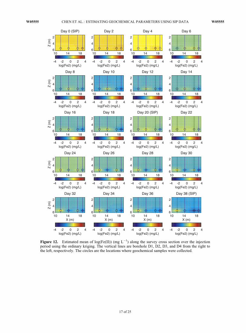
Figure 12. Estimated mean of log(Fe(II)) (mg L�1) along the survey cross section over the injectionperiod using the ordinary kriging. The vertical lines are borehole D1, D2, D3, and D4 from the right tothe left, respectively. The circles are the locations where geochemical samples were collected.

W05555 CHEN ET AL.: ESTIMATING GEOCHEMICAL PARAMETERS USING SIP DATA W05555

17 of 25

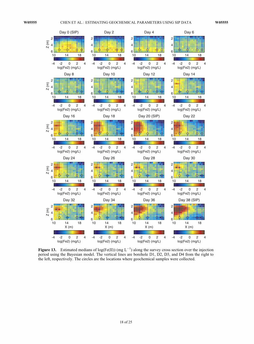
Figure 13. Estimated medians of log(Fe(II)) (mg L�1) along the survey cross section over the injectionperiod using the Bayesian model. The vertical lines are borehole D1, D2, D3, and D4 from the right tothe left, respectively. The circles are the locations where geochemical samples were collected.

W05555 CHEN ET AL.: ESTIMATING GEOCHEMICAL PARAMETERS USING SIP DATA W05555

18 of 25

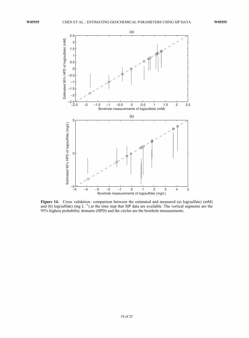
Figure 14. Cross validation: comparison between the estimated and measured (a) log(sulfate) (mM)and (b) log(sulfide) (mg L�1) at the time step that SIP data are available. The vertical segments are the95% highest probability domains (HPD) and the circles are the borehole measurements.

W05555 CHEN ET AL.: ESTIMATING GEOCHEMICAL PARAMETERS USING SIP DATA W05555

19 of 25

Figure 15. Cross validation: comparison between the estimated and measured log(sulfate) (mM) at (a)borehole D1, (b) borehole D2, (c) borehole D3, and (d) borehole D4 over the injection period. The RMSof the differences between the measured and the estimated values for Bayesian and kriging methods are0.57 and 0.69, respectively.

W05555 CHEN ET AL.: ESTIMATING GEOCHEMICAL PARAMETERS USING SIP DATA W05555

20 of 25

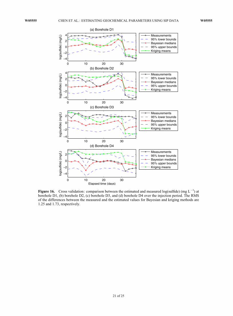
Figure 16. Cross validation: comparison between the estimated and measured log(sulfide) (mg L�1) atborehole D1, (b) borehole D2, (c) borehole D3, and (d) borehole D4 over the injection period. The RMSof the differences between the measured and the estimated values for Bayesian and kriging methods are1.25 and 1.73, respectively.

W05555 CHEN ET AL.: ESTIMATING GEOCHEMICAL PARAMETERS USING SIP DATA W05555

21 of 25

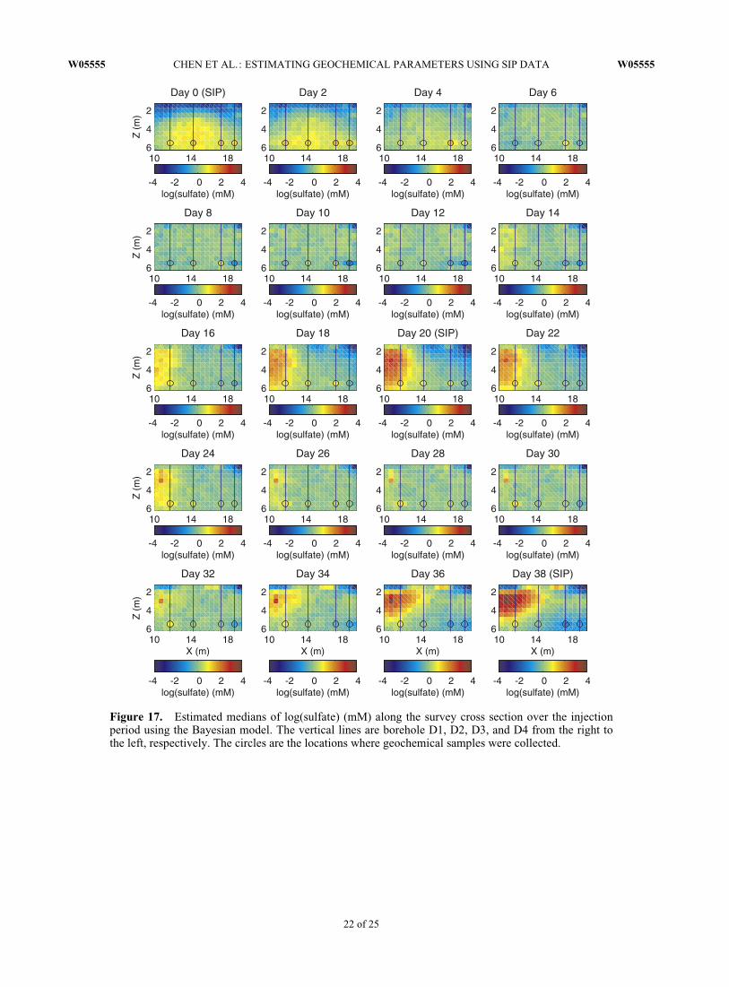
Figure 17. Estimated medians of log(sulfate) (mM) along the survey cross section over the injectionperiod using the Bayesian model. The vertical lines are borehole D1, D2, D3, and D4 from the right tothe left, respectively. The circles are the locations where geochemical samples were collected.

W05555 CHEN ET AL.: ESTIMATING GEOCHEMICAL PARAMETERS USING SIP DATA W05555

22 of 25

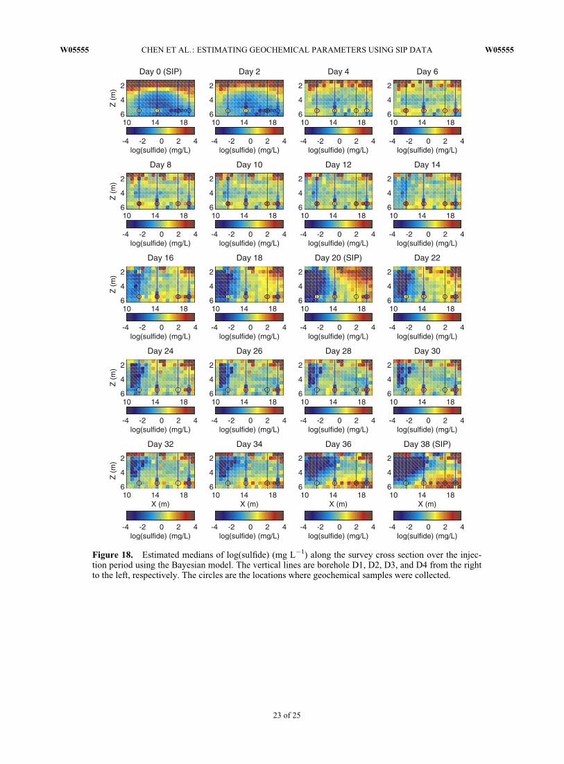
Figure 18. Estimated medians of log(sulfide) (mg L�1) along the survey cross section over the injec-tion period using the Bayesian model. The vertical lines are borehole D1, D2, D3, and D4 from the rightto the left, respectively. The circles are the locations where geochemical samples were collected.

W05555 CHEN ET AL.: ESTIMATING GEOCHEMICAL PARAMETERS USING SIP DATA W05555

23 of 25

in modern hydrogeological studies. In particular, this studyshows the possibility to solve for Cole-Cole parametersrequired for the application of petrophysical models asdeveloped in laboratory studies.

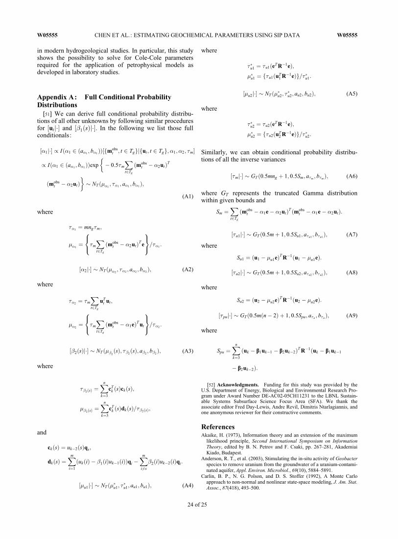
Appendix A: Full Conditional ProbabilityDistributions

[51] We can derive full conditional probability distribu-tions of all other unknowns by following similar proceduresfor ½utj�� and ½�1ðsÞj��. In the following we list those fullconditionals:

½�1j�� / Ið�1 2 ða�1 ; b�1ÞÞ½fmobst ; t 2 Tggjfut; t 2 Tgg; �1; �2; �m�

/ Ið�1 2 ða�1 ; b�1ÞÞexp

�� 0:5�m

Xt2Tg

ðmobst � �2utÞT

ðmobst � �2utÞ

�� NT ð��1

; ��1 ; a�1 ; b�1Þ;

(A1)

where

��1 ¼ mng�m;

��1¼ �m

Xt2Tg

ðmobst � �2utÞT e

8<:

9=;=��1 :

½�2j�� � NT ð��2; ��2 ; a�2 ; b�2Þ; (A2)

where

��2 ¼ �m

Xt2Tg

uTt ut;

��2¼ �m

Xt2Tg

ðmobst � �1eÞT ut

8<:

9=;=��2 :

½�2ðsÞj�� � NT ð��2ðsÞ; ��2

ðsÞ; a�2; b�2Þ; (A3)

where

��2ðsÞ ¼Xn

k¼3

cTk ðsÞckðsÞ;

��2ðsÞ ¼Xn

k¼3

cTk ðsÞdkðsÞ=��2ðsÞ;

and

ckðsÞ ¼ uk�2ðsÞqs;

dkðsÞ ¼Xm

i¼1

ðukðiÞ � �1ðiÞuk�1ðiÞÞqi �Xm

i6¼s

�2ðiÞuk�2ðiÞqi:

½�u1j�� � NT ð��u1; ��u1; au1; bu1Þ; (A4)

where

��u1 ¼ �u1ðeT R�1eÞ;��u1 ¼ f�u1ðuT

1 R�1eÞg=��u1:

½�u2j�� � NT ð��u2; ��u2; au2; bu2Þ; (A5)

where

��u2 ¼ �u2ðeT R�1eÞ;��u2 ¼ f�u2ðuT

2 R�1eÞg=��u2:

Similarly, we can obtain conditional probability distribu-tions of all the inverse variances

½�mj�� � GT ð0:5mng þ 1; 0:5Sm; a�m ; b�mÞ; (A6)

where GT represents the truncated Gamma distributionwithin given bounds and

Sm ¼Xt2Tg

ðmobst � �1e� �2utÞT ðmobs

t � �1e� �2utÞ:

½�u1j�� � GT ð0:5mþ 1; 0:5Su1; a�u1 ; b�u1Þ; (A7)

where

Su1 ¼ ðu1 � �u1eÞT R�1ðu1 � �u1eÞ:

½�u2j�� � GT ð0:5mþ 1; 0:5Su2; a�u2 ; b�u2Þ; (A8)

where

Su2 ¼ ðu2 � �u2eÞT R�1ðu2 � �u2eÞ:

½�puj�� � GT ð0:5mðn� 2Þ þ 1; 0:5Spu; a�u ; b�uÞ; (A9)

where

Spu ¼Xn

k¼3

ðuk � b1uk�1 � b2uk�2ÞT R�1ðuk � b1uk�1

� b2uk�2Þ:

[52] Acknowledgments. Funding for this study was provided by theU.S. Department of Energy, Biological and Environmental Research Pro-gram under Award Number DE-AC02-05CH11231 to the LBNL Sustain-able Systems Subsurface Science Focus Area (SFA). We thank theassociate editor Fred Day-Lewis, Andre Revil, Dimitris Ntarlagiannis, andone anonymous reviewer for their constructive comments.

ReferencesAkaike, H. (1973), Information theory and an extension of the maximum

likelihood principle, Second International Symposium on InformationTheory, edited by B. N. Petrov and F. Csaki, pp. 267–281, AkademiaiKiado, Budapest.

Anderson, R. T., et al. (2003), Stimulating the in-situ activity of Geobacterspecies to remove uranium from the groundwater of a uranium-contami-nated aquifer, Appl. Environ. Microbiol., 69(10), 5884–5891.

Carlin, B. P., N. G. Polson, and D. S. Stoffer (1992), A Monte Carloapproach to non-normal and nonlinear state-space modeling, J. Am. Stat.Assoc., 87(418), 493–500.

24 of 25

W05555 CHEN ET AL.: ESTIMATING GEOCHEMICAL PARAMETERS USING SIP DATA W05555

Chen, J., A. Kemna, and S. S. Hubbard (2008), A comparison betweenGauss-Newton and Markov chain Monte Carlo based methods for invert-ing spectral induced polarization data for Cole-Cole parameters, Geophy-sics, 73(6), F247–F259.

Chen, J., S. Hubbard, K. Williams, S. Pride, L. Li, C. Steefel, and L. Slater(2009), A state-space Bayesian framework for estimating biogeochemi-cal transformations using time-lapse geophysical data, Water Resour.Res., 45, W08420, doi:10.1029/2008WR007698.

Commer, M., G. A. Newman, K. H. Williams, and S. S. Hubbard (2011),3D induced-polarization data inversion for complex resistivity, Geophy-sics, 76(3), F157–F171.

Cosenza, P., A. Ghorbani, N. Florsch, and A. Revil (2007), Effects of dry-ing on the low-frequency electrical properties of Tournemire argillites,Pure Appl. Geophys., 164(10), 2043–2066.

Englert, A., S. S. Hubbard, K. H. Williams, L. Li, and C. I. Steefel (2009),Feedbacks between hydrological heterogeneity and bioremediation inducedbiogeochemical transformations, Environ. Sci. Technol., 43, 5197–5204.

Flores Orozco, A., K. H. Williams, P. E. Long, S. S. Hubbard, andA. Kemna (2011), Using complex resistivity imaging to infer biogeochem-ical processes associated with bioremediation of an uranium contaminatedaquifer, J. Geophys. Res., 116, G03001, doi:10.1029/2010JG001591.

Gelfand. A. E., and F. M. Smith (1990), Sampling-based approaches to cal-culating marginal densities, J. Am. Stat. Assoc., 85(410), 398–409.

Gelman, S., and D. Gelman (1984), Stochastic relaxation, Gibbs distribu-tion, and Bayesian restoration of images, IEEE Trans. Pattern Anal.Mach. Intel., 6, 721–741.

Johnson, T. C., R. J. Versteeg, A. Ward, F. D. Day-Lewis, and A. Revil(2010), Improved hydrogeophysical characterization and monitoringthrough high performance electrical geophysical modeling and inversion,Geophysics, 75(4), WA27–WA41.

Karaoulis, M., A. Revil, D. D. Werkema, B. J. Minsley, W. F. Woodruff,and A. Kemna (2011), Time-lapse three-dimensional inversion of com-plex conductivity data using an active time constrained (ATC) approach,Geophys. J. Int., 187, 237–251.

Kemna, A. (2000), Tomographic inversion of complex resistivity: Theoryand application, Ph.D. thesis, Ruhr-University, Bochum.

Kitanidis, P. K. (1997), Introduction to Geostatistics: Applications inHydrogeology, Cambridge University Press, New York.

Kohavi, R. (1995), A study of cross-validation and bootstrap for accuracyestimation and model selection, International Joint Conference on Artifi-cial Intelligence, Morgan Kaufmann Publ., San Francisco, Calif.

Li, L., C. I. Steefel, M. B. Kowalsky, A. Englert, and S. Hubbard(2010), Effects of physical and geochemical heterogeneities on mineraltransformation and biomass accumulation during biostimulation experi-ments at Rifle, Colorado, J. Contam. Hydrol., 112, 45–63.

Lorenz, J. C. (1982), Sedimentology of the Mesaverde formation at Riflegap, Colorado and implications for gas-bearing intervals in the subsur-face, Report SAND82-0604, Sandia National Laboratory, Albuquerque,N.M., 43 pp.

Lovley, D. R., F. H. Chapelle, and J. C. Woodward (1994), Use of dissolvedH2 concentrations to determine distribution of microbially catalyzed

redox reactions in anoxic groundwater, Environ. Sci. Technol., 28,1205–1210.

Ntarlagiannis, D., K. H. Williams, L. Slater, and S. S. Hubbard (2005),Low-frequency electrical response to microbial induced sulfide precipita-tion, J. Geophys. Res., 110, G02009, doi:10.1029/2005JG000024.

Olhoeft, G. (1992), Geophysical detection of hydrocarbon and organicchemical contaminants, 587–594, SAGEEP, proceedings, Oakbrook, IL.

Personna, Y. R., D. Ntarlagiannis, L. Slater, N. Yee, M. O’Brien, and S. S.Hubbard (2008), Spectral induced polarization and electrodic potentialmonitoring of microbially mediated iron sulfide transformations, J. Geo-phys. Res., 113, G02020, doi:10.1029/2007JG000614.

Revil, A., and M. Skold (2011), Salinity dependence of spectral inducedpolarization in sands and sandstones, Geophys. J. Int., 187, 813–824.

Slater, L., D. Ntarlagiannis, and D. Wishart (2006), On the relationshipbetween induced polarization and surface area in metal-sand and clay-sand mixtures, Geophysics, 71, A1–A5.

Slater, L., D. Ntarlagiannis, Y. R. Personna, and S. Hubbard (2007), Pore-scale spectral induced polarization signatures associated with FeS bio-mineral transformations, Geophys. Res. Lett., 34, L21404, doi:10.1029/2007GL031840.

Sogade, J. A., F. Scri-Scappuzzo, Y. Vichabian, W. Shi, W. Rodi, D. P.Lesmes, and F. D. Morgan (2006), Induced-polarization detection andmapping of contaminant plumes, Geophysics, 71(3), B75.

Vanhala, H. (1997), Mapping oil-contaminated sand and till with the spec-tral induced polarization (SIP) method, Geophys. Prospecting, 45, P303–P326.

Vrionis, H. A., R. T. Anderson, I. Ortiz-Bernad, K. R. O’Neill, C. T. Resch,A. D. Peacock, R. Dayvault, D. C. White, P. E. Long, and D. R. Lovley(2005), Microbiological and geochemical heterogeneity in an in situ ura-nium bioremediation field site, Appl. Environ. Microbiol., 71(10), 6308–6318.

Wikle, C. K. (2003), Hierarchical Bayesian models for predicting thespread of ecological processes, Ecology, 84, 1384–1394.

Williams, K. H., D. Ntarlagiannis, L. D. Slater, A. Dohnalkova, S. S. Hub-bard, and J. F. Banfield (2005), Geophysical imaging of stimulated mi-crobial biomineralization, Eviron. Sci. Technol., 39, 7592–7600.

Williams, K. H., A. Kemna, M. Wilkins, J. Druhan, E. Arntzen, L. N0Guessan,P. E. Long, S. S. Hubbard, and J. F. Banfield (2009), Geophysical monitor-ing of coupled microbial and geochemical processes during stimulated sub-surface bioremediation, Environ. Sci. Technol., 43(17), 6717–6723,doi:10.1021/es900855j.

Williams, K. H., et al. (2011), Acetate availability and its influence on sus-tainable bioremediation of uranium-contaminated groundwater. Geomi-crobiol. J., 28, 519–539. doi:10.1080/01490451.2010.520074.

Wu, Y., J. Ajo-Franklin, N. Spycher, S. Hubbard, G. Zhang, K. H. Williams,J. Taylor, Y. Fujita, and R. Smith (2011), Geophysical monitoring and re-active transport modeling of ureolytically driven calcium carbonate precip-itation, Geochem. Trans., 12(7), 1–20.

Yabusaki, S. B., et al. (2007), Uranium removal from groundwater via in-situ bioremediation: Field-scale modeling of transport and biologicalprocesses, J. Contam. Hydrol., 93, 216–235.

25 of 25

W05555 CHEN ET AL.: ESTIMATING GEOCHEMICAL PARAMETERS USING SIP DATA W05555