Estimating the free gas content in Baltic Sea sediments using compressional wave velocity from marine seismic data

Journal of Geophysical Research: Solid Earth

RESEARCH ARTICLE10.1002/2014JB010989

Key Points:• Velocities from high-resolution

seismic data can be used to quantifyshallow gas

• Gas volume fraction in thegas-charged Holocene mud is anaverage 0.046%

• Free gas occurs vertically throughoutmost of the Holocene mud inthe Baltic

Correspondence to:Zs. Tóth,[email protected]

Citation:Tóth, Zs., V. Spiess, J. M. Mogollón, andJ. B. Jensen (2014), Estimating the freegas content in Baltic Sea sedimentsusing compressional wave velocityfrom marine seismic data, J. Geophys.Res. Solid Earth, 119, 8577–8593,doi:10.1002/2014JB010989.

Received 27 JAN 2014

Accepted 8 OCT 2014

Accepted article online 18 OCT 2014

Published online 5 DEC 2014

Estimating the free gas content in Baltic Sea sediments usingcompressional wave velocity from marine seismic dataZsuzsanna Tóth1, Volkhard Spiess1, José M. Mogollón2, and Jørn Bo Jensen3

1Department of Geosciences, University of Bremen, Bremen, Germany, 2Department of Earth Sciences - Geochemistry,Utrecht University, Utrecht, Netherlands, 3Geological Survey of Denmark and Greenland, Copenhagen, Denmark

Abstract A 2-D high-resolution velocity field was obtained from marine seismic data to quantify freegas content in shallow muddy sediments at in situ pressure and temperature. The velocities were acquiredapplying Migration Velocity Analysis on prestack time-migrated data. Compressional wave velocities arehighly sensitive to free gas as very small amounts of gas can cause a significant decrease in the mediumvelocity. The analyzed profile crosses a depression filled with organic-rich Holocene mud in the BornholmBasin, Baltic Sea. The interval velocity field reveals two low-velocity patches, which extend from the reversedpolarity reflections marking the top of the gassy sediment layer down to the base of the Holocene mud.Average interval velocities within the gassy mud are lower than the seafloor migration velocity by up to∼500 m/s. This decrease, using a geoacoustic model, is caused by an average 0.046% gas volume fraction.The interval velocities in individual cells of the velocity field are reduced to ∼200 m/s predicting up to 3.4%gas content. The velocity field is limited in resolution due to velocity determination at and betweenreflections; however, together with the stratigraphic interpretation, geological units containing free gascould be identified. Shallow gas occurs vertically throughout most of the Holocene mud in the gassy area.Comparison with biogeochemical studies at other Baltic Sea sites suggests that the distribution of freegas is likely to be patchy in the sediment, but the gas concentration may peak below the sulfate-methanetransition zone and gradually decrease below.

1. Introduction

In fine-grained sediments, methane (CH4) is commonly produced by microbes through the degradation oforganic matter. This potent greenhouse gas can be found in large amounts in unconsolidated marine sed-iments worldwide. Most of the methane is effectively broken down in the subsurface, either aerobicallyin the presence of oxygen [Reeburgh, 1969] or consumed by microorganisms in a process called anaero-bic methane oxidation (AOM), which occurs in the sulphate-methane transition zone (SMTZ) [Sansone andMartens, 1978; Reeburgh, 2007; Boetius et al., 2000; Milucka et al., 2012]. Below the SMTZ, however, dissolvedmethane in the pore water can accumulate to levels which exceed supersaturation. Under low pressures andhigh temperatures typical of nonpolar continental shelves, once the partial pressure of CH4 overcomes theambient hydrostatic pressure, free methane gas forms as discrete bubbles.

Observations in Baltic Sea sediments suggest that free gas formation occurs in the organic-rich mud thathas been deposited in the Baltic Sea since its opening to the North Sea roughly 9.8 ka [Andrén et al., 2011].Free gas has been observed in locations where this mud layer exceeds 5 to 10 m in thickness [Thießen et al.,2006; Jensen and Bennike, 2009]. The accumulation of CH4 gas in the sediment therefore seems to be largelycontrolled by sedimentation rate and the flux of organic matter to the seafloor [Mogollón et al., 2012].

Little is known about the amount, vertical distribution, and migration of gas bubbles in gas-bearing marinesediments. Observational evidence provided by acoustic measurements is often restricted to imaging asnapshot in time. High-frequency sediment echosounders provide the most suitable technique for thedetection and mapping of shallow gas, because acoustic signals are distinctly attenuated by the scatteringof gas bubbles [e.g., Judd and Hovland, 1992]. Regions of shallow, gas-bearing sediments appear impenetra-ble in acoustic profiles, thus often blank or turbid in acoustic facies. Extensive areas of acoustic blanking andturbidity were reported and mapped in many areas of the Baltic Sea using high-frequency sources [Mathyset al., 2005; Thießen et al., 2006; Laier and Jensen, 2007; Majewski and Klusek, 2011]. As a consequence ofthe strong attenuation, however, acoustic profilers often only image the upper boundary of the gassy

TÓTH ET AL. ©2014. American Geophysical Union. All Rights Reserved. 8577

Journal of Geophysical Research: Solid Earth 10.1002/2014JB010989

sediment (gas front on top of the acoustic blanking zones) and fail to provide information about the verticaldistribution of gas. Computed tomography (CT) scans of ∼5 m long pressurized cores from Eckernförde Bay(Western Baltic Sea) showed that the bubble distribution in the sediment is not uniform and that gas bub-bles exist within 2 to 20 cm thick intervals which are separated by gas-free intervals [Abegg and Anderson,1997; Anderson et al., 1998].

Transport of methane in the sediment can occur by diffusion (in the fluid phase), advection of the porewater [Albert et al., 1998], or advection driven by the buoyancy of gas bubbles. Gas bubbles formed atdepth may either become trapped or migrate toward the sediment-water interface [Tréhu et al., 2004; Liuand Flemings, 2006]. Indirect evidence of bubble migration include the observation of seeps – gas bubblesrising up through the water column [e.g., Judd, 2004], and migration pathways observed on seismo-acousticdata, e.g., columnar disturbances and gas chimneys [e.g., Judd and Hovland, 1992]. Mechanisms for gas bub-ble formation and migration within “impermeable” mud are currently subject to debate. Gas injections intogelatine and mud showed that bubbles grow as highly eccentric oblate spheroids (disks) by fracturing thecohesive host medium or by reopening preexisting fractures [Boudreau et al., 2005]. Likewise, computersimulations suggest that sediment fracturing may also trigger bubble rise [Algar et al., 2011]; however,the estimated rising speeds of bubbles may be unrealistically high [Boudreau, 2012].

The quantity of free gas in the sediment is difficult to measure, because methane degasses when the sedi-ment is brought to ambient pressure during core recovery. Pressurized core samplers, which could maintainthe in situ gas content, are often not long enough, expensive and only rarely used [e.g., Best et al., 2004]. Asimple technique for measuring in situ gas concentration would thus have great advantages. In deep seasediments, hydrate and free gas contents have been previously estimated using seismic velocities [Lee et al.,1993, 1996; Wood et al., 1994; Ecker et al., 2000]. At low (seismic) frequencies, a small amount of free gas inthe sediment reduces compressional wave velocity significantly [Anderson and Hampton, 1980b]. The acous-tic impedance contrast between the fully water saturated and the gas-bearing sediment layers results in areversed polarity reflector in marine seismic profiles. Based on a reduction of compressional wave veloc-ity in gassy sediments, in situ amounts of free gas may be estimated using the velocity field obtained fromseismic data.

Our goals in this study, using a 2-D shallow seismic profile from the Bornholm Basin, Baltic Sea, are(1) to investigate shallow gas-bearing sediments and the geological background of free gas formation,(2) to obtain compressional wave (seismic) velocity and estimate the free gas content in the sediment, and(3) to characterize the vertical distribution of gas bubbles in the sediment.

2. Bornholm Basin

The Bornholm Basin is located in the southern Baltic Sea, northeast of Bornholm island (Denmark), andsouthwest of mainland Sweden (Figure 1). This sub-basin of the Baltic Sea is situated in a major structuraldepression that subsided during the deposition of Upper Cretaceous sediments [Sviridov et al., 1995]. Thepre-Quaternary bedrock in the basin consists mainly of these late Mesozoic limestones topped with anunconformity surface, and the Quaternary basin fill is composed of a unit of glacial deposits, overlain by asuccession of late- and post-glacial lacustrine and marine sediments [Kögler and Larsen, 1979].

After the last deglaciation of the Baltic Sea basin, isostatic uplift together with eustatic sea-level changesresulted in four to five distinct phases of sedimentation [Björk, 1995; Andrén et al., 2011] (Figure 2). In theBaltic Ice Lake stage (BIL, 16.0–11.7 ka BP), glacial (varved) clays and silt were deposited conformably onthe rugged pre-Quaternary surface shaped by glacial deformation and on top of the glacial till. The partlybrackish Yoldia Sea stage (11.7–10.7 ka BP) and the fresh-water Ancylus Lake stage (10.7–9.8 ka BP) werecharacterized by the deposition of homogeneous clays (AY clays), which together with the BIL clays form analmost continuous cover over the deeper part of the eastern Bornholm Basin [Kögler and Larsen, 1979]. Thebeginning of the subsequent brackish Littorina Sea stage (9.8 ka BP) is a sharp litostratigraphic boundarywith a change to deposition of fine-grained mud, rich in organic matter. The organic carbon content (TOC)measured in core samples shows an increase from the start of the initial Littorina Sea stage and has a max-imum in the end of post-Littorina Sea (6–7%) [Andrén et al., 2000]. The transition to the recent Baltic Seastage (circa 800 B.P. to present) is recorded as a biostratigraphical change in the mud [Andrén et al., 2000].

TÓTH ET AL. ©2014. American Geophysical Union. All Rights Reserved. 8578

Journal of Geophysical Research: Solid Earth 10.1002/2014JB010989

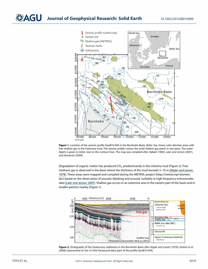
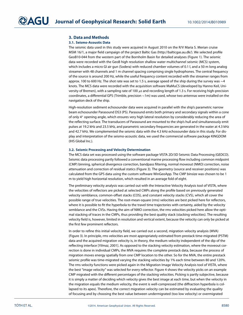
Figure 1. Location of the seismic profile GeoB10-044 in the Bornholm Basin, Baltic Sea. Green color denotes areas withfree shallow gas in the Holocene mud. The seismic profile crosses the small shallow gas patch in two parts. The waterdepth is given in meter next to the contour lines. The map was compiled after Vejbæk [1985], Laier and Jensen [2007],and Graversen [2009].

Degradation of organic matter has produced CH4 predominantly in the Littorina mud (Figure 2). Freemethane gas is observed in the basin where the thickness of the mud exceeds 5–10 m [Kögler and Larsen,1979]. These areas were mapped and compiled during the METROL project (http://metrol.mpi-bremen.de/) based on the observation of acoustic blanking and acoustic turbidity in high-frequency echosounderdata [Laier and Jensen, 2007]. Shallow gas occurs in an extensive area in the eastern part of the basin and insmaller patches nearby (Figure 1).

Figure 2. Stratigraphy of the Quaternary sediments in the Bornholm Basin after Kögler and Larsen [1979]; Andrén et al.[2000] represented on the 4.3 kHz Parasound data (part of the profile GeoB10-044).

TÓTH ET AL. ©2014. American Geophysical Union. All Rights Reserved. 8579

Journal of Geophysical Research: Solid Earth 10.1002/2014JB010989

3. Data and Methods3.1. Seismo-Acoustic DataThe seismic data used in this study were acquired in August 2010 on the R/V Maria S. Merian cruiseMSM 16/1, a major field campaign of the project Baltic Gas (http://balticgas.au.dk/). We selected profileGeoB10-044 from the western part of the Bornholm Basin for detailed analyses (Figure 1). The seismicdata were recorded with the GeoB high resolution shallow water multichannel seismic (MCS) system,which includes a micro GI air gun (Sodera) with reduced chamber volumes of 0.1 l, and a 50 m long analogstreamer with 48 channels and 1 m channel spacing comprising single hydrophones. The central frequencyof the source is around 200 Hz, while the useful frequency content recorded with the streamer ranges fromapprox. 100 to 600 Hz. The shot rate was set to 1.5 s, average speed of the ship during the survey was ∼4knots. The MCS data were recorded with the acquisition software MaMuCS (developed by Hanno Keil, Uni-versity of Bremen), with a sampling rate of 100 𝜇s and recording length of 1.3 s. For receiving high-precisioncoordinates, a differential GPS (Trimble, precision ∼1m) was used, whose two antennas were installed on thenavigation deck of the ship.

High-resolution sediment echosounder data were acquired in parallel with the ship’s parametric narrowbeam echosounder Parasound DS3 (PS). Parasound emits both primary and secondary signals within a coneof only 4◦ opening angle, which ensures very high lateral resolution by considerably reducing the area ofthe reflecting surface. The transducers of Parasound are mounted to the ship’s hull and simultaneously emitpulses at 19.2 kHz and 23.5 kHz, and parametric secondary frequencies are generated in the water at 4.3 kHzand 42.7 kHz. We complemented the seismic data with the 4.3 kHz echosounder data in this study. For dis-play and interpretation of the seismo-acoustic data, we used the commercial software package KINGDOM(IHS Global Inc.).

3.2. Seismic Processing and Velocity DeterminationThe MCS data set was processed using the software package VISTA 2D/3D Seismic Data Processing (GEDCO).Seismic data processing partly followed a conventional marine processing flow including common midpoint(CMP) binning, spherical divergence correction, bandpass filtering, normal moveout (NMO) correction, noiseattenuation and correction of residual statics (Figure 3). The geometry (source and receiver positions) wascalculated from the GPS data using the custom software WinGeoApp. The CMP binsize was chosen to be 1m to yield high horizontal resolution, which resulted in an average fold of eight.

The preliminary velocity analysis was carried out with the Interactive Velocity Analysis tool of VISTA, wherethe velocities of reflectors are picked at selected CMPs along the profile based on previously generatedvelocity semblance, common-offset stacks (COS), and constant velocity stacks (CVS), which all cover thepossible range of true velocities. The root-mean-square (rms) velocities are best picked here for reflectors,where it is possible to fit the hyperbola to the travel time trajectories with certainty, aided by the velocitysemblance and the CVSs. Having the aim of NMO correction, the rms velocities picked here allow the opti-mal stacking of traces in the CMPs, thus providing the best quality stack (stacking velocities). The resultingvelocity field is, however, limited in resolution and vertical extent, because the velocity can only be picked atthe first few prominent reflectors.

In order to refine this initial velocity field, we carried out a second, migration velocity analysis (MVA)(Figure 3). In principle, rms velocities are most appropriately estimated from prestack time-migrated (PSTM)data and the acquired migration velocity is, in theory, the medium velocity independent of the dip of thereflecting interface [Yilmaz, 2001]. As opposed to the stacking velocity estimation, where the moveout cor-rection is done in individual CMPs, the MVA requires the complete prestack data, because the process ofmigration moves energy spatially from one CMP location to the other. So for the MVA, the entire prestackseismic profile was time-migrated varying the stacking velocities by 1% each time between 80 and 120%.The rms velocity functions were picked again in the Migration Image Velocity Analysis tool of VISTA, wherethe best “image velocity” was selected for every reflector. Figure 4 shows the velocity picks on an exampleCMP migrated with the different percentages of the stacking velocities. Picking is partly subjective, becauseit is simply a matter of deciding which velocity gives the best image at each time, but when the velocity inthe migration equals the medium velocity, the event is well-compressed (the diffraction hyperbola is col-lapsed to its apex). Therefore, the correct migration velocity can be estimated by evaluating the qualityof focusing and by choosing the best value between undermigrated (too low velocity) or overmigrated

TÓTH ET AL. ©2014. American Geophysical Union. All Rights Reserved. 8580

Journal of Geophysical Research: Solid Earth 10.1002/2014JB010989

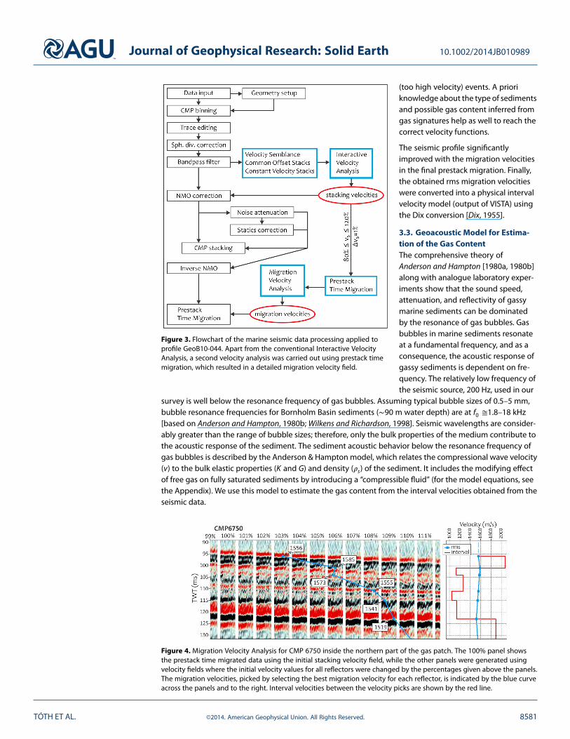
Figure 3. Flowchart of the marine seismic data processing applied toprofile GeoB10-044. Apart from the conventional Interactive VelocityAnalysis, a second velocity analysis was carried out using prestack timemigration, which resulted in a detailed migration velocity field.

(too high velocity) events. A prioriknowledge about the type of sedimentsand possible gas content inferred fromgas signatures help as well to reach thecorrect velocity functions.

The seismic profile significantlyimproved with the migration velocitiesin the final prestack migration. Finally,the obtained rms migration velocitieswere converted into a physical intervalvelocity model (output of VISTA) usingthe Dix conversion [Dix, 1955].

3.3. Geoacoustic Model for Estima-tion of the Gas ContentThe comprehensive theory ofAnderson and Hampton [1980a, 1980b]along with analogue laboratory exper-iments show that the sound speed,attenuation, and reflectivity of gassymarine sediments can be dominatedby the resonance of gas bubbles. Gasbubbles in marine sediments resonateat a fundamental frequency, and as aconsequence, the acoustic response ofgassy sediments is dependent on fre-quency. The relatively low frequency ofthe seismic source, 200 Hz, used in our

survey is well below the resonance frequency of gas bubbles. Assuming typical bubble sizes of 0.5–5 mm,bubble resonance frequencies for Bornholm Basin sediments (∼90 m water depth) are at f0 ≅1.8–18 kHz[based on Anderson and Hampton, 1980b; Wilkens and Richardson, 1998]. Seismic wavelengths are consider-ably greater than the range of bubble sizes; therefore, only the bulk properties of the medium contribute tothe acoustic response of the sediment. The sediment acoustic behavior below the resonance frequency ofgas bubbles is described by the Anderson & Hampton model, which relates the compressional wave velocity(v) to the bulk elastic properties (K and G) and density (𝜌s) of the sediment. It includes the modifying effectof free gas on fully saturated sediments by introducing a “compressible fluid” (for the model equations, seethe Appendix). We use this model to estimate the gas content from the interval velocities obtained from theseismic data.

Figure 4. Migration Velocity Analysis for CMP 6750 inside the northern part of the gas patch. The 100% panel showsthe prestack time migrated data using the initial stacking velocity field, while the other panels were generated usingvelocity fields where the initial velocity values for all reflectors were changed by the percentages given above the panels.The migration velocities, picked by selecting the best migration velocity for each reflector, is indicated by the blue curveacross the panels and to the right. Interval velocities between the velocity picks are shown by the red line.

TÓTH ET AL. ©2014. American Geophysical Union. All Rights Reserved. 8581

Journal of Geophysical Research: Solid Earth 10.1002/2014JB010989

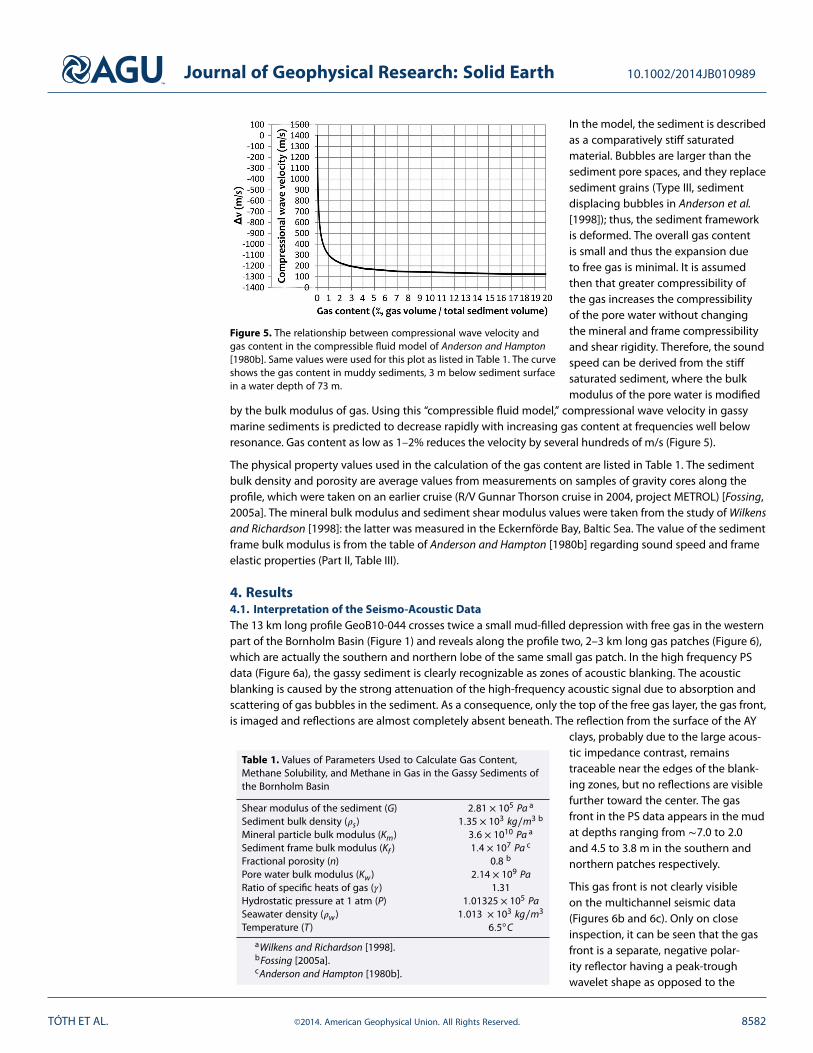
Figure 5. The relationship between compressional wave velocity andgas content in the compressible fluid model of Anderson and Hampton[1980b]. Same values were used for this plot as listed in Table 1. The curveshows the gas content in muddy sediments, 3 m below sediment surfacein a water depth of 73 m.

In the model, the sediment is describedas a comparatively stiff saturatedmaterial. Bubbles are larger than thesediment pore spaces, and they replacesediment grains (Type III, sedimentdisplacing bubbles in Anderson et al.[1998]); thus, the sediment frameworkis deformed. The overall gas contentis small and thus the expansion dueto free gas is minimal. It is assumedthen that greater compressibility ofthe gas increases the compressibilityof the pore water without changingthe mineral and frame compressibilityand shear rigidity. Therefore, the soundspeed can be derived from the stiffsaturated sediment, where the bulkmodulus of the pore water is modified

by the bulk modulus of gas. Using this “compressible fluid model,” compressional wave velocity in gassymarine sediments is predicted to decrease rapidly with increasing gas content at frequencies well belowresonance. Gas content as low as 1–2% reduces the velocity by several hundreds of m/s (Figure 5).

The physical property values used in the calculation of the gas content are listed in Table 1. The sedimentbulk density and porosity are average values from measurements on samples of gravity cores along theprofile, which were taken on an earlier cruise (R/V Gunnar Thorson cruise in 2004, project METROL) [Fossing,2005a]. The mineral bulk modulus and sediment shear modulus values were taken from the study of Wilkensand Richardson [1998]: the latter was measured in the Eckernförde Bay, Baltic Sea. The value of the sedimentframe bulk modulus is from the table of Anderson and Hampton [1980b] regarding sound speed and frameelastic properties (Part II, Table III).

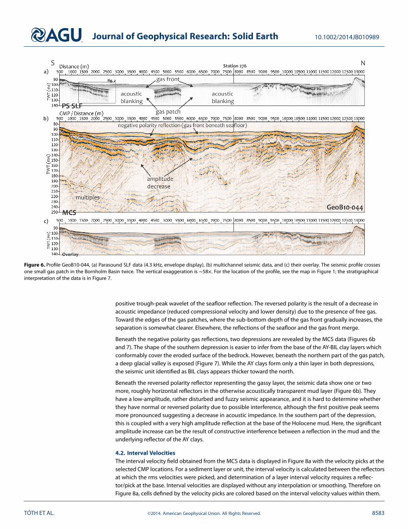
4. Results4.1. Interpretation of the Seismo-Acoustic DataThe 13 km long profile GeoB10-044 crosses twice a small mud-filled depression with free gas in the westernpart of the Bornholm Basin (Figure 1) and reveals along the profile two, 2–3 km long gas patches (Figure 6),which are actually the southern and northern lobe of the same small gas patch. In the high frequency PSdata (Figure 6a), the gassy sediment is clearly recognizable as zones of acoustic blanking. The acousticblanking is caused by the strong attenuation of the high-frequency acoustic signal due to absorption andscattering of gas bubbles in the sediment. As a consequence, only the top of the free gas layer, the gas front,is imaged and reflections are almost completely absent beneath. The reflection from the surface of the AY

Table 1. Values of Parameters Used to Calculate Gas Content,Methane Solubility, and Methane in Gas in the Gassy Sediments ofthe Bornholm Basin

Shear modulus of the sediment (G) 2.81 × 105 Pa a

Sediment bulk density (𝜌s) 1.35 × 103 kg∕m3 b

Mineral particle bulk modulus (Km) 3.6 × 1010 Pa a

Sediment frame bulk modulus (Kf ) 1.4 × 107 Pa c

Fractional porosity (n) 0.8 b

Pore water bulk modulus (Kw) 2.14 × 109 PaRatio of specific heats of gas (𝛾) 1.31Hydrostatic pressure at 1 atm (P) 1.01325 × 105 PaSeawater density (𝜌w) 1.013 × 103 kg∕m3

Temperature (T) 6.5◦C

aWilkens and Richardson [1998].bFossing [2005a].cAnderson and Hampton [1980b].

clays, probably due to the large acous-tic impedance contrast, remainstraceable near the edges of the blank-ing zones, but no reflections are visiblefurther toward the center. The gasfront in the PS data appears in the mudat depths ranging from ∼7.0 to 2.0and 4.5 to 3.8 m in the southern andnorthern patches respectively.

This gas front is not clearly visibleon the multichannel seismic data(Figures 6b and 6c). Only on closeinspection, it can be seen that the gasfront is a separate, negative polar-ity reflector having a peak-troughwavelet shape as opposed to the

TÓTH ET AL. ©2014. American Geophysical Union. All Rights Reserved. 8582

Journal of Geophysical Research: Solid Earth 10.1002/2014JB010989

Figure 6. Profile GeoB10-044, (a) Parasound SLF data (4.3 kHz, envelope display), (b) multichannel seismic data, and (c) their overlay. The seismic profile crossesone small gas patch in the Bornholm Basin twice. The vertical exaggeration is ∼58×. For the location of the profile, see the map in Figure 1; the stratigraphicalinterpretation of the data is in Figure 7.

positive trough-peak wavelet of the seafloor reflection. The reversed polarity is the result of a decrease inacoustic impedance (reduced compressional velocity and lower density) due to the presence of free gas.Toward the edges of the gas patches, where the sub-bottom depth of the gas front gradually increases, theseparation is somewhat clearer. Elsewhere, the reflections of the seafloor and the gas front merge.

Beneath the negative polarity gas reflections, two depressions are revealed by the MCS data (Figures 6band 7). The shape of the southern depression is easier to infer from the base of the AY-BIL clay layers whichconformably cover the eroded surface of the bedrock. However, beneath the northern part of the gas patch,a deep glacial valley is exposed (Figure 7). While the AY clays form only a thin layer in both depressions,the seismic unit identified as BIL clays appears thicker toward the north.

Beneath the reversed polarity reflector representing the gassy layer, the seismic data show one or twomore, roughly horizontal reflectors in the otherwise acoustically transparent mud layer (Figure 6b). Theyhave a low-amplitude, rather disturbed and fuzzy seismic appearance, and it is hard to determine whetherthey have normal or reversed polarity due to possible interference, although the first positive peak seemsmore pronounced suggesting a decrease in acoustic impedance. In the southern part of the depression,this is coupled with a very high amplitude reflection at the base of the Holocene mud. Here, the significantamplitude increase can be the result of constructive interference between a reflection in the mud and theunderlying reflector of the AY clays.

4.2. Interval VelocitiesThe interval velocity field obtained from the MCS data is displayed in Figure 8a with the velocity picks at theselected CMP locations. For a sediment layer or unit, the interval velocity is calculated between the reflectorsat which the rms velocities were picked, and determination of a layer interval velocity requires a reflec-tor/pick at the base. Interval velocities are displayed without any interpolation or smoothing. Therefore onFigure 8a, cells defined by the velocity picks are colored based on the interval velocity values within them.

TÓTH ET AL. ©2014. American Geophysical Union. All Rights Reserved. 8583

Journal of Geophysical Research: Solid Earth 10.1002/2014JB010989

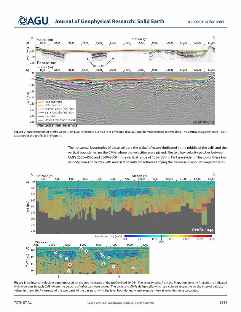
Figure 7. Interpretation of profile GeoB10-044, (a) Parasound SLF (4.3 kHz, envelope display), and (b) multichannel seismic data. The vertical exaggeration is ∼58×.Location of the profile is in Figure 1.

The horizontal boundaries of these cells are the picks/reflectors (indicated in the middle of the cell), and thevertical boundaries are the CMPs where the velocities were picked. The two low velocity patches betweenCMPs 2500–4500 and 5500–8500 in the vertical range of 105–130 ms TWT are evident. The top of these lowvelocity zones coincides with reversed polarity reflections verifying the decrease in acoustic impedance as

Figure 8. (a) Interval velocities superimposed on the seismic traces of the profile GeoB10-044. The velocity picks from the Migration Velocity Analysis are indicatedwith blue dots in each CMP where the velocity of reflectors were picked. The picks and CMPs define cells, which are colored respective to the interval velocityvalues in them. (b) A close-up of the two parts of the gas patch with the layer boundaries, where average interval velocities were calculated.

TÓTH ET AL. ©2014. American Geophysical Union. All Rights Reserved. 8584

Journal of Geophysical Research: Solid Earth 10.1002/2014JB010989

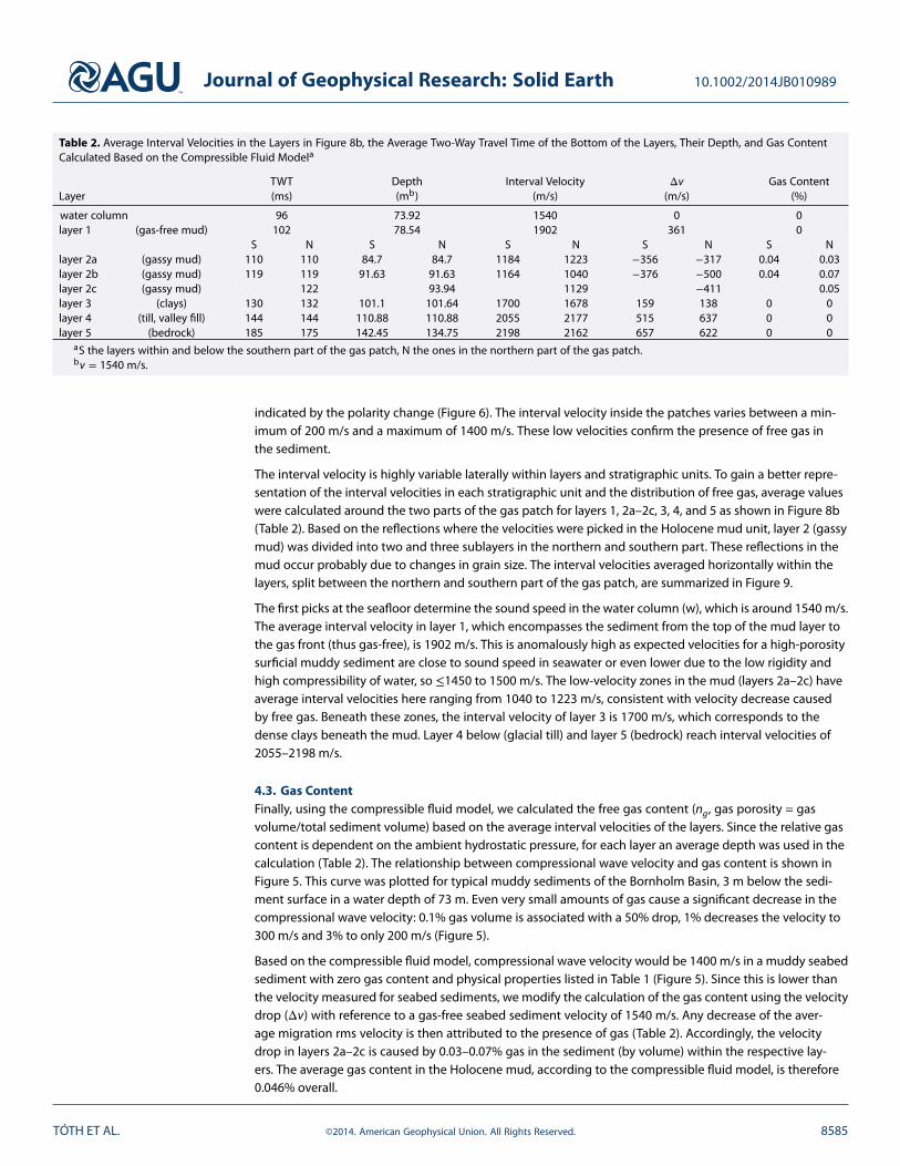
Table 2. Average Interval Velocities in the Layers in Figure 8b, the Average Two-Way Travel Time of the Bottom of the Layers, Their Depth, and Gas ContentCalculated Based on the Compressible Fluid Modela

TWT Depth Interval Velocity Δv Gas ContentLayer (ms) (mb) (m/s) (m/s) (%)

water column 96 73.92 1540 0 0layer 1 (gas-free mud) 102 78.54 1902 361 0

S N S N S N S N S Nlayer 2a (gassy mud) 110 110 84.7 84.7 1184 1223 −356 −317 0.04 0.03layer 2b (gassy mud) 119 119 91.63 91.63 1164 1040 −376 −500 0.04 0.07layer 2c (gassy mud) 122 93.94 1129 −411 0.05layer 3 (clays) 130 132 101.1 101.64 1700 1678 159 138 0 0layer 4 (till, valley fill) 144 144 110.88 110.88 2055 2177 515 637 0 0layer 5 (bedrock) 185 175 142.45 134.75 2198 2162 657 622 0 0

aS the layers within and below the southern part of the gas patch, N the ones in the northern part of the gas patch.bv = 1540 m/s.

indicated by the polarity change (Figure 6). The interval velocity inside the patches varies between a min-imum of 200 m/s and a maximum of 1400 m/s. These low velocities confirm the presence of free gas inthe sediment.

The interval velocity is highly variable laterally within layers and stratigraphic units. To gain a better repre-sentation of the interval velocities in each stratigraphic unit and the distribution of free gas, average valueswere calculated around the two parts of the gas patch for layers 1, 2a–2c, 3, 4, and 5 as shown in Figure 8b(Table 2). Based on the reflections where the velocities were picked in the Holocene mud unit, layer 2 (gassymud) was divided into two and three sublayers in the northern and southern part. These reflections in themud occur probably due to changes in grain size. The interval velocities averaged horizontally within thelayers, split between the northern and southern part of the gas patch, are summarized in Figure 9.

The first picks at the seafloor determine the sound speed in the water column (w), which is around 1540 m/s.The average interval velocity in layer 1, which encompasses the sediment from the top of the mud layer tothe gas front (thus gas-free), is 1902 m/s. This is anomalously high as expected velocities for a high-porositysurficial muddy sediment are close to sound speed in seawater or even lower due to the low rigidity andhigh compressibility of water, so ≤1450 to 1500 m/s. The low-velocity zones in the mud (layers 2a–2c) haveaverage interval velocities here ranging from 1040 to 1223 m/s, consistent with velocity decrease causedby free gas. Beneath these zones, the interval velocity of layer 3 is 1700 m/s, which corresponds to thedense clays beneath the mud. Layer 4 below (glacial till) and layer 5 (bedrock) reach interval velocities of2055–2198 m/s.

4.3. Gas ContentFinally, using the compressible fluid model, we calculated the free gas content (ng, gas porosity = gasvolume/total sediment volume) based on the average interval velocities of the layers. Since the relative gascontent is dependent on the ambient hydrostatic pressure, for each layer an average depth was used in thecalculation (Table 2). The relationship between compressional wave velocity and gas content is shown inFigure 5. This curve was plotted for typical muddy sediments of the Bornholm Basin, 3 m below the sedi-ment surface in a water depth of 73 m. Even very small amounts of gas cause a significant decrease in thecompressional wave velocity: 0.1% gas volume is associated with a 50% drop, 1% decreases the velocity to300 m/s and 3% to only 200 m/s (Figure 5).

Based on the compressible fluid model, compressional wave velocity would be 1400 m/s in a muddy seabedsediment with zero gas content and physical properties listed in Table 1 (Figure 5). Since this is lower thanthe velocity measured for seabed sediments, we modify the calculation of the gas content using the velocitydrop (Δv) with reference to a gas-free seabed sediment velocity of 1540 m/s. Any decrease of the aver-age migration rms velocity is then attributed to the presence of gas (Table 2). Accordingly, the velocitydrop in layers 2a–2c is caused by 0.03–0.07% gas in the sediment (by volume) within the respective lay-ers. The average gas content in the Holocene mud, according to the compressible fluid model, is therefore0.046% overall.

TÓTH ET AL. ©2014. American Geophysical Union. All Rights Reserved. 8585

Journal of Geophysical Research: Solid Earth 10.1002/2014JB010989

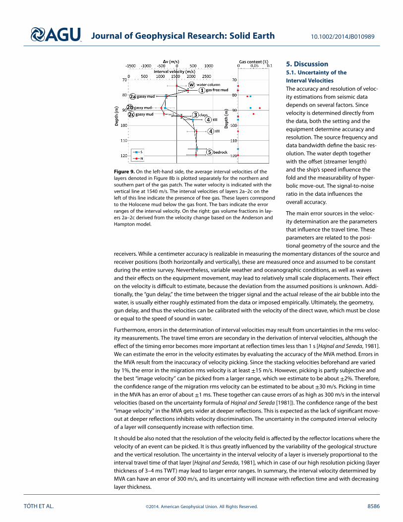
Figure 9. On the left-hand side, the average interval velocities of thelayers denoted in Figure 8b is plotted separately for the northern andsouthern part of the gas patch. The water velocity is indicated with thevertical line at 1540 m/s. The interval velocities of layers 2a–2c on theleft of this line indicate the presence of free gas. These layers correspondto the Holocene mud below the gas front. The bars indicate the errorranges of the interval velocity. On the right: gas volume fractions in lay-ers 2a–2c derived from the velocity change based on the Anderson andHampton model.

5. Discussion5.1. Uncertainty of theInterval VelocitiesThe accuracy and resolution of veloc-ity estimations from seismic datadepends on several factors. Sincevelocity is determined directly fromthe data, both the setting and theequipment determine accuracy andresolution. The source frequency anddata bandwidth define the basic res-olution. The water depth togetherwith the offset (streamer length)and the ship’s speed influence thefold and the measurability of hyper-bolic move-out. The signal-to-noiseratio in the data influences theoverall accuracy.

The main error sources in the veloc-ity determination are the parametersthat influence the travel time. Theseparameters are related to the posi-tional geometry of the source and the

receivers. While a centimeter accuracy is realizable in measuring the momentary distances of the source andreceiver positions (both horizontally and vertically), these are measured once and assumed to be constantduring the entire survey. Nevertheless, variable weather and oceanographic conditions, as well as wavesand their effects on the equipment movement, may lead to relatively small scale displacements. Their effecton the velocity is difficult to estimate, because the deviation from the assumed positions is unknown. Addi-tionally, the “gun delay,” the time between the trigger signal and the actual release of the air bubble into thewater, is usually either roughly estimated from the data or imposed empirically. Ultimately, the geometry,gun delay, and thus the velocities can be calibrated with the velocity of the direct wave, which must be closeor equal to the speed of sound in water.

Furthermore, errors in the determination of interval velocities may result from uncertainties in the rms veloc-ity measurements. The travel time errors are secondary in the derivation of interval velocities, although theeffect of the timing error becomes more important at reflection times less than 1 s [Hajnal and Sereda, 1981].We can estimate the error in the velocity estimates by evaluating the accuracy of the MVA method. Errors inthe MVA result from the inaccuracy of velocity picking. Since the stacking velocities beforehand are variedby 1%, the error in the migration rms velocity is at least ±15 m/s. However, picking is partly subjective andthe best “image velocity” can be picked from a larger range, which we estimate to be about ±2%. Therefore,the confidence range of the migration rms velocity can be estimated to be about ±30 m/s. Picking in timein the MVA has an error of about ±1 ms. These together can cause errors of as high as 300 m/s in the intervalvelocities (based on the uncertainty formula of Hajnal and Sereda [1981]). The confidence range of the best“image velocity” in the MVA gets wider at deeper reflections. This is expected as the lack of significant move-out at deeper reflections inhibits velocity discrimination. The uncertainty in the computed interval velocityof a layer will consequently increase with reflection time.

It should be also noted that the resolution of the velocity field is affected by the reflector locations where thevelocity of an event can be picked. It is thus greatly influenced by the variability of the geological structureand the vertical resolution. The uncertainty in the interval velocity of a layer is inversely proportional to theinterval travel time of that layer [Hajnal and Sereda, 1981], which in case of our high resolution picking (layerthickness of 3–4 ms TWT) may lead to larger error ranges. In summary, the interval velocity determined byMVA can have an error of 300 m/s, and its uncertainty will increase with reflection time and with decreasinglayer thickness.

TÓTH ET AL. ©2014. American Geophysical Union. All Rights Reserved. 8586

Journal of Geophysical Research: Solid Earth 10.1002/2014JB010989

5.2. Variability in the Interval VelocitiesBased on our MVA, the migration rms velocity of the seafloor reflection (and thus the interval velocity/soundspeed in the water column) is 50–100 m/s higher than sound velocity measured near the seabed from CTDcasts (1459 m/s) [Schneider von Deimling et al., 2013]. Although the reasons are unclear, our higher migrationvelocities at the seafloor may indicate that the values of the entire velocity field are higher than the realmedium velocity values.

The anomalously high average interval velocity of layer 1, corresponding to gas-free mud at the seabed,likely shows the effect of thin layers on the interval velocity. Compressional wave velocity in gas-free muddyseabed of the Eckernförde Bay, Baltic Sea (similar environment and sediment) was measured in situ usingan acoustic lance and it was found to be 1430–1480 m/s [Fu et al., 1996; Wilkens and Richardson, 1998]. The∼400 m/s deviation here is probably attributable to rms velocity picks at too close time intervals, whichcan yield anomalous interval velocities from the Dix conversion, even though the increase in rms velocitywith depth is small [Yilmaz, 2001]. For example, in the case of rms velocities of 1500 and 1550 m/s at the topand base of a 3 m thick layer (4 ms TWT), the interval velocity is 2452 m/s. Therefore, the 1902 m/s intervalvelocity of layer 1 is a consequence of the vertically high resolution velocity picking and the derivation ofthe interval velocity, and it does not characterize the sediment layer between the bounding rms velocitypicks. Similarly, the interval velocity can be anomalously low when the bounding rms velocity picks are tooclose to each other and the rms velocity decreases too sharply between the two picks. To avoid the thinlayer problem or the too sharp decrease of the rms velocity, we ran tests to investigate the reliability of theinterval velocity values by removing velocity picks within the gassy sediment. These showed that the lowestvelocities inside the gassy mud are not anomalous. Nevertheless, it is important to note that as the layerthickness decreases, the uncertainty in its interval velocity will increase.

The interval velocities within layers/stratigraphic units (Figure 8a) appear highly variable. This variability canresult from the method of velocity determination and/or could reflect small changes in the sediment lithol-ogy, gas content, etc. While such significant changes in lithology within stratigraphic units are not likely inBornholm Basin sediments, variations in layer thickness and depth can result in slightly different intervalvelocities. In the Dix conversion, the underlying assumption is that the earth model comprises horizontalisovelocity layers. Therefore, decreasing layer thicknesses lead to increasing interval velocities and largeruncertainties in the computed interval velocities of the deeper layers. As a consequence, the interval veloc-ity determined between closely spaced reflectors in a complex geological structure will likely result in highlyvariable values.

Apart from this, variability in the distribution, amount, and concentration of gas bubbles may also causesubtle changes in the compressional wave velocity. Abegg and Anderson [1997] found in the EckernfördeBay sediments that gas bubble distributions are variable vertically on a centimeter scale (thin gassy andnongassy layers a few cm thick in 5 m long cores) and horizontally on a meter scale (from cores collected2–20 m apart). Actual gas volume concentrations measured in cores kept under in situ pressure and tem-perature using the CT scanning technique revealed highly variable free gas concentrations, from 0.1% to9%, changing both vertically and laterally [Abegg and Anderson, 1997; Anderson et al., 1998]. This means thatalternating layers of low and high velocities in the sediment are likely [Wilkens and Richardson, 1998]. Whilehigh concentrations of gas bubbles represent small heterogeneities in the medium when compared to thewavelength of the seismic wave (the wavelength λ∼7.5 m for the 200 Hz signal of the airgun), given thehigh sensitivity of compressional wave velocities to changing gas content (Figure 5), thin gassy sedimentlayers can cause considerable variability in the interval velocities. Measured velocities thus represent anaverage of lower velocities in gassy sediments and higher velocities in gas-free sediments.

5.3. Velocity Reduction–Gas ContentGardner [2000] performed controlled experiments on silty clay samples prepared in the laboratory contain-ing 1–2% gas volume with a uniform distribution of 0.2–1.8 mm sized gas bubbles. The acoustic responseof the gassy sediments was broadly as predicted by the compressible fluid model, with measurements ofcompressional wave velocities as low as 220 m/s below the resonance frequency of the bubbles. However, asubsequent study by Gardner and Sills [2001] revealed that velocities based on bulk properties of sedimentscontaining “large bubbles” match the actual velocity measurements better than velocities based on the pre-dictions of the compressible fluid model. In the “large bubble model,” gas is contained in structural pocketsin the saturated sediment [Wheeler, 1988; Wheeler and Gardner, 1989]. This is probably a more appropriate

TÓTH ET AL. ©2014. American Geophysical Union. All Rights Reserved. 8587

Journal of Geophysical Research: Solid Earth 10.1002/2014JB010989

physical description of gas-bearing sediments, as typical gas bubbles are bigger than clay or silt particlesand cannot be wholly contained within the pore water in typical fine-grained sediments. The large bub-bles have a lower compressibility than the small bubbles formed within the fluid. Consequently, the velocityreduction due to free gas happens to a lesser degree, because the abrupt increase in the bulk compressibil-ity is smaller (equation (A1) in the Appendix). This means that the reduction in the interval velocities mightbe caused by an even larger amount of gas in the sediment than the compressible fluid model suggests(for more detail, see Gardner and Sills [2001]). Our calculated free gas contents may thus represent a lowerestimate of gas contents.

Dvorkin and Nur [1998] considered different saturation patterns in partially saturated sediments and rocks.In their model, patchy gas saturation as opposed to the homogeneous pattern, is a pore fluid arrangementwhere the fluid (free gas) is arranged in fully saturated patches that are surrounded by dry (nongassy) orpartially saturated regions. The gas saturation can be therefore heterogeneous on scales greater than thepore or grain size but on scales smaller than the seismic wavelength. If the gas saturation is patchy in theHolocene mud, then again much higher gas concentrations would be predicted from the low-velocity zones,because the increase in the bulk compressibility of the sediment is smaller than in case of a heterogeneousfluid saturation.

5.4. Gas Distribution and Amount in Bornholm Basin SedimentsThe depth distribution of gas bubbles in the sediment is difficult to evaluate, because information about thefree gas zone derived from seismo-acoustic data is limited. In the PS profiles, the top of the free gas zone ismarked by the strongly scattering gas front, but due to the strong attenuation of the high-frequency signal,nothing deeper can be inferred from inside the acoustic blanking zones (Figure 6a). In the lower frequencyseismic data, a horizon at the same depth as the gas front in PS data appears as a reversed polarity reflection(Figure 6b), and although penetration through the gassy layer is achieved, the base of the gas-charged sed-iment layer is difficult to identify. If the gas bubbles are concentrated in a thin layer, it might not be possibleto resolve the layer boundaries as separate reflections. If the gas bubbles are distributed in a thicker layer,but with a gradual decrease of gas bubble concentration with depth, then again only one reflection may beobserved, which would then mark the top of the gas-charged sediment layer. The gradual increase of veloc-ity and/or density (gradient zone) in the medium will not cause a sharp acoustic impedance contrast; thus,reflection amplitude may be much lower than expected from the total impedance contrast.

The interval velocity field determined from the MCS data (Figure 8a) reveals presence of free gas through thereduction of compressional wave velocity (v < 1540 m/s, blue colors). Low interval velocities characterize theHolocene mud layer beneath the gas front. The velocity drop is confined to the mud (layers 2a–2c), whereasthe clays below (layer 3) show higher interval velocities well above 1540 m/s (Figure 8b and Table 2). Thissuggests that gas bubbles are present throughout the Holocene mud beneath the gas front. The velocitiesfor all layers represent average values for these units and thus do not take into account any intralayer ver-tical variations and inhomogeneities. Also, the long seismic wavelength and the vertical uncertainty of thereflector picks limit the velocity resolution for thin layers. Accordingly, the velocity drop with respect to thevelocity in gas-free sediment (the reference value) probably indicates average free gas content. The aver-age interval velocities in layers 2a–2c suggest that in the northern part of the gas patch the highest free gasconcentrations occur in the middle of the mud unit. This is not well resolved in the southern part of the gaspatch, where the two layers in the mud unit appear to have similar gas contents.

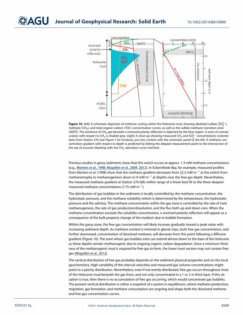
Multicore data retrieved from the northern part of the gas patch [Station 276, latitude: 55.317950◦N, lon-gitude: 15.028730◦E, water depth: 73.2 m, Fossing, 2005b] reveal that the SMTZ is located at a depth ofapprox. 30 cm below seafloor (Figure 10). This SMTZ depth is not uncommon for gassy sediments in theBaltic Sea and is similar to SMTZ depths compiled at Eckernförde Bay [Mogollón et al., 2011, and referencestherein], and Arkona Basin [Mogollón et al., 2012]. The reversed polarity reflector at Station 276 for the freegas depth occurs at 2.68 m below seafloor. The in situ pressure, temperature, and salinity conditions at thissediment depth lead to a methane solubility concentration of 16.4 mM [Mogollón et al., 2013]. Combin-ing this information, a methane gradient between the deepest methane measurement and the free gasdepth is estimated to be 6.9 mM m−1 (Figure 10). This gradient is considerably less than that obtained fromlinearly interpolating the two deepest methane concentration (10.5 mM m−1). This discrepancy is due tothe dynamics of methanogenic and methanotrophic processes, with the steepest portion of the methanecurve taking place at the change from net methanogenesis to net methanotrophy [Mogollón et al., 2009].

TÓTH ET AL. ©2014. American Geophysical Union. All Rights Reserved. 8588

Journal of Geophysical Research: Solid Earth 10.1002/2014JB010989

Figure 10. (left) A schematic depiction of methane cycling within the Holocene mud, showing idealized sulfate (SO2−4 ),

methane (CH4), and total organic carbon (TOC) concentration curves, as well as the sulfate-methane transition zone(SMTZ). The existence of CH4 gas beneath a reversed polarity reflection is depicted by the blue region. A zone of oversat-uration with respect to CH4 is shaded grey. (right) A close-up showing measured CH4 and SO2−

4 concentrations (coloreddots) from Station 276 (see Figure 1 for location), put into context with the schematic panel to the left. A methane con-centration gradient with respect to depth is predicted by linking the deepest measurement point to the intersection ofthe top of acoustic blanking with the CH4 saturation curve (red line).

Previous studies in gassy sediments show that this switch occurs at approx. 1-3 mM methane concentrations[e.g., Martens et al., 1998; Mogollón et al., 2009, 2012]. In Eckernförde Bay, for example, measured profilesfrom Martens et al. [1998] show that the methane gradient decreases from 22.3 mM m−1 at the switch frommethanotrophy to methanogenesis down to 9 mM m−1 at depths near the free gas depth. Nevertheless,the measured methane gradient at Station 276 falls within range of a linear best fit to the three deepestmeasured methane concentrations (7.75 mM m−1).

The distribution of gas bubbles in the sediment is locally controlled by the methane concentration, thehydrostatic pressure, and the methane solubility (which is determined by the temperature, the hydrostaticpressure and the salinity). The methane concentration within the gas zone is controlled by the rate of (net)methanogenesis, the rate of gas production/dissolution, and the flux both up and down core. When themethane concentration exceeds the solubility concentration, a reversed polarity reflection will appear as aconsequence of the bulk property change of the medium due to bubble formation.

Within the gassy zone, the free gas concentration will likely increase gradually toward a peak value withincreasing sediment depth. As methane content is minimal in glacial clays, both free gas concentration, andfurther downward, concentration of dissolved methane, will decrease from this point following a diffusivegradient (Figure 10). The zone where gas bubbles exist can extend almost down to the base of the Holoceneas these depths remain methanogenic due to ongoing organic carbon degradation. Since a minimum thick-ness of the methanogenic mud is required for free gas to form, the lower most section may not contain freegas [Mogollón et al., 2012].

The vertical distribution of free gas probably depends on the sediment physical properties and on the localgeochemistry. High variability of the interval velocities and measured gas volume concentrations mightpoint to a patchy distribution. Nevertheless, even if not evenly distributed, free gas occurs throughout mostof the Holocene mud beneath the gas front, and not only concentrated in a 1 or 2 m thick layer. If this sit-uation is true, then there is no accumulation of free gas occurring, which would concentrate gas bubbles.The present vertical distribution is rather a snapshot of a system in equilibrium, where methane production,migration, gas formation, and methane consumption are ongoing and shape both the dissolved methaneand free gas concentration curves.

TÓTH ET AL. ©2014. American Geophysical Union. All Rights Reserved. 8589

Journal of Geophysical Research: Solid Earth 10.1002/2014JB010989

The average gas content of 0.046% for the Holocene mud from our calculation is comparable with theresults of other studies from the Baltic Sea. Methane gas concentrations at in situ pressure and temperaturehave been measured in the muddy sediments of Eckernförde Bay. Over the depth zone of 50 to 120 cm, ata water depth of 26 m, the average gas concentration was found to be approx. 0.02% [Abegg and Anderson,1997; Anderson et al., 1998; Martens et al., 1998]. Modeling studies by Martens et al. [1998] and Albert et al.[1998], which quantitatively couple the biogeochemical processes to the input flux of reactive organic car-bon in the sediment, predicted gas concentrations of ∼0.3%, for essentially the same depth zone where thegas bubbles were observed in the pressurized cores. Mogollón et al. [2011] used a reactive transport modelto investigate the seasonal dynamics of the methane cycle. Their model predicted (depth-averaged) gas vol-ume fractions of 0.25% for the early fall months in the Eckernförde Bay sediments, and early spring valueswere as low as 0.021%. This model study also indicated that there can be considerable variations in the posi-tion and thickness of the free gas layer due to the seasonal fluctuations of heat propagation. This needs tobe taken into account when comparing measured values of free gas concentration.

In our study, the interval velocities in individual cells of the velocity field are reduced to 201 and 262 m/s inthe southern and northern part of the gas patch, respectively. This predicts up to 3.4% and 1.6% gas contentin the volumes of the sediment bounded by the rms velocity picks. These values seem high compared to theaverage gas content, but not unlikely, as pressurized cores from the pockmark site in the Eckernförde Bayreached concentrations as high as 9%. Based on model predictions, Mogollón et al. [2011] argues that highfree gas concentrations are unlikely near the gas front due to seasonal production and migration of freemethane gas. Deeper gas layers may thus be a product of gas burial and concentration over a long period oftime [Mogollón et al., 2012].

Given our estimated average gas concentration based on seismic velocities, it is possible to predict gas vol-umes on a more regional scale if we assume that our gas content estimate is representative of the entiregas patch area. Imposing the average gas contents, depths and thicknesses for the gassy zone (layers 2a–2c,Table 2), as well as the sediment properties listed in Table 1, a depth-integrated quantity of 2.8 mol m−2

can be estimated for the methane gas present. Nevertheless, this value probably represents a low estimatesince the model does not capture small-sized bubbles (also see discussion in section 5.3). If this value is rep-resentative for the entire gas patch area of 15.25 km2, then around 43 Mmol methane would be harboredin the Holocene mud as free gas, or roughly 1.1 × 106 m3 of methane at standard ambient temperatureand pressure. While this constitutes a small fraction in comparison to the global methane hydrate inventory[1017 − 1018 mol C, Dickens, 2011], it is evaluated over a gassy patch that represents only 0.00005% of theglobal shelf (0-200 m water depth) extent. Given the prolific evidence for free methane gas in these shal-low sediments [Fleischer et al., 2011], we may expect that the yet unreported free gas inventory can be asignificant part of the global methane reservoir.

6. Conclusions

We performed detailed velocity analyses on a 2-D shallow marine seismic profile from the Bornholm Basin,Baltic Sea. Although it is time consuming and computationally intensive, migration velocity analysis offers amethod to obtain high-resolution velocity fields from prestack time migrated data. Beyond ensuring accu-rate geometry and travel times in the seismic data, precise velocity determination is important, as smallerrors in the migration rms velocities can result in large errors in the interval velocities.

The seismic profile GeoB10-044 crosses a small depression filled with organic-rich Holocene mud, whereshallow free gas is observed. Free gas in the sediment is indicated by acoustic blanking zones on thehigh-frequency acoustic data, and the same horizon as the gas front appears as a reversed polarity reflec-tion on the lower frequency seismic data. The interval velocities obtained from the seismic data revealtwo low-velocity zones along the profile, which extend from the reversed polarity reflections down to thebase of the Holocene mud layer. Average interval velocity values within the gassy mud are lower than theseafloor migration velocity by up to 500 m/s. This decrease in interval velocity, using the geoacoustic modelof Anderson and Hampton [1980b] that relates compressional wave velocity to sediment physical proper-ties and gas content, is caused by an average 0.046% gas fraction in the sediment. Compressional wavevelocities in the sediment are highly sensitive to free gas, and very small amounts of gas cause a signifi-cant decrease in the medium velocity at seismic frequencies. Based on the seismo-acoustic data and the

TÓTH ET AL. ©2014. American Geophysical Union. All Rights Reserved. 8590

Journal of Geophysical Research: Solid Earth 10.1002/2014JB010989

derived interval velocities, shallow gas occurs vertically throughout most of the Holocene mud. Althoughthe distribution of free gas is patchy in the sediment, the gas concentration is likely to have a peak belowthe sulphate-methane transition zone and gradually decreases below.

Interval velocities obtained from multichannel seismic data can be used for the assessment of free gasconcentration at in situ pressure and temperature in shallow marine sediments. The measurement of thevelocity reduction caused by free gas is possible even when only a small amount (>0.01%) of free gas ispresent in the sediment. The high-resolution velocity field offers the opportunity to investigate the freegas distribution with depth as well. Although limited in resolution because of the requirement of reflectors,together with the stratigraphic interpretation of the seismic data, geological units containing free gas can beidentified. Due to the frequency dependence of gas-bearing sediments and the seismic method, relativelylow source frequency is needed, which is well below the resonance frequency of gas bubbles and providespenetration through the gassy sediment layer, but sufficiently high as to provide high vertical resolution inthe imaging of the subsurface.

Appendix A: Geoacoustic Model

The relationship between compressional wave velocity and the physical and elastic properties ofgas-bearing sediments at acoustic frequencies much less than the bubble resonance frequency is given bythe following equations after Anderson and Hampton [1980b] and Wilkens and Richardson [1998].

Compressional wave velocity in gas-bearing sediments is given by the wave equation:

v =

√√√√K + 43

G

𝜌s, (A1)

where K is the bulk modulus of the gas-bearing sediment, G is the sediment shear modulus, and 𝜌s isthe sediment bulk density. The sediment composite bulk modulus is calculated based on Gassmann’sexpressions [Gassmann, 1951]:

K = Km

(Kf + Q′

Km + Q′

), (A2)

where

Q′ = K ′w

(Km − Kf

n(

Km − K ′w

)). (A3)

Here Km and Kf are the mineral and frame bulk moduli, n is the fractional porosity, and the bulk modulus ofthe pore water (Kw) is modified by the addition of gas (K ′

w), introducing a compressible pore fluid:

K ′w =

KwKg

n′gKg +

(1 − n′

g

)Kg

. (A4)

In case of adiabatic compression, the bulk modulus of the gas is Kg = 𝛾P0, where 𝛾 is the ratio of specificheats of gas and P0 is the ambient hydrostatic pressure. The fraction of sediment pore space occupied bygas (n′

g) is the gas volume (ng) divided by the fractional porosity (n):

n′g =

ng

n. (A5)

ReferencesAbegg, F., and A. L. Anderson (1997), The acoustic turbid layer in muddy sediments of Eckernförde Bay, Western Baltic: Methane

concentration, saturation and bubble characteristics, Mar. Geol., 137, 137–147.Albert, D. B., C. S. Martens, and M. J. Alperin (1998), Biogeochemical processes controlling methane in gassy coastal sediments—Part 2:

Groundwater flow control of acoustic turbidity in Eckernförde Bay sediments, Cont. Shelf Res., 18, 1771–1793.Algar, C. K., B. P. Boudreau, and M. A. Barry (2011), Initial rise of bubble in cohesive sediments by a process of viscoelastic fracture,

J. Geophys. Res., 116, B04207, doi:10.1029/2010JB008133.Anderson, A. L., and L. D. Hampton (1980a), Acoustics of gas-bearing sediments. I. Background, J. Acoust. Soc. Am., 67, 1865–1889.

AcknowledgmentsWe wish to thank Niklas Allroggenand Marius Becker for their help withMatlab and Sabine Flury for usefulcomments on an early draft of themanuscript. We would like to thankthe editor and two anonymous review-ers for their helpful and constructivecomments that greatly contributedto improving the final version of themanuscript. This research was part ofthe Baltic Gas project and received thefunding from the European Commu-nity’s Seventh Framework Programme(FP/2007-2013) under grant agree-ment 217246 made with the jointBaltic Sea research and developmentprogram BONUS. The educationaluser-license grant of IHS Global Inc.and the support of GEDCO allowedus to use the softwares The KingdomSuite and VISTA 2D/3D SeismicData Processing.

TÓTH ET AL. ©2014. American Geophysical Union. All Rights Reserved. 8591

Journal of Geophysical Research: Solid Earth 10.1002/2014JB010989

Anderson, A. L., and L. D. Hampton (1980b), Acoustics of gas-bearing sediments. II. Measurements and models, J. Acoust. Soc. Am., 67,1890–1903.

Anderson, A. L., F. Abegg, J. A. Hawkins, M. E. Duncan, and E. P. Lyons (1998), Bubble populations and acoustic interaction with the gassyfloor of Eckernförde Bay, Cont. Shelf Res., 18, 1807–1839.

Andrén, E., T. Andrén, and G. Sohlenius (2000), The Holocene history of the southwestern Baltic Sea as reflected in a sediment core fromthe Bornholm Basin, Boreas, 19, 233–250.

Andrén, T., S. Björk, E. Andrén, D. Conley, L. Zillén, and J. Anjar (2011), Development of the Baltic Sea Basin during the last 130 ka,in The Baltic Sea Basin, Central and Eastern European Development Studies (CEEDES), edited by J. Harff et al., pp. 75–97, Springer,Berlin Heidelberg.

Best, A. I., M. D. J. Tuffin, J. K. Dix, and J. M. Bull (2004), Tidal height and frequency dependence of acoustic velocity and attenuation inshallow gassy marine sediments, J. Geophys. Res., 109, B08101, doi:10.1029/2003JB002748.

Björk, S. (1995), A review of the history of the Baltic Sea, 13.0–8.0 ka BP, Quat. Int., 27, 19–40.Boetius, A., K. Ravenschlag, C. J. Schubert, D. Rickert, F. Widdel, A. Gieseke, R. Amann, B. B. Jorgensen, U. Witte, and U. Pfannkuche (2000),

A marine microbial consortium apparently mediating anaerobic oxidation of methane, Nature, 407, 623–626.Boudreau, B. P. (2012), The physics of bubbles in surficial, soft, cohesive sediments, Mar. Pet. Geol., 38, 1–18.Boudreau, B. P., C. Algar, B. D Johnson, I. Croudace, A. Reed, Y. Furukawa, K. M. Dorgan, P. A. Jumars, A. S. Grader, and B. S. Gardiner

(2005), Bubble growth and rise in soft sediments, Geology, 33, 517–520.Dickens, G. R. (2011), Down the rabbit hole: Toward appropriate discussion of methane release from gas hydrate systems during the

Paleocene-Eocene thermal maximum and other past hyperthermal events, Clim. Past, 7, 831–846.Dix, C. H. (1955), Seismic velocities from surface measurements, Geophysics, 20, 68–86.Dvorkin, J., and A. Nur (1998), Acoustic signatures of patchy saturation, Int. J. Solids Struct., 35, 4803–4810.Ecker, C., J. Dvorkin, and A. M. Nur (2000), Estimating the amount of gas-hydrate and free gas from marine data, Geophysics, 65, 565–573.Fleischer, P., T. H. Orsi, M. D. Richardson, and A. L. Anderson (2011), Distribution of free gas in marine sediments: A global overview,

Geo-Mar. Lett., 21, 103–122.Fossing, H. (2005a), Biogeochemistry and physical properties in core GT04-314G, PANGAEA, doi:10.1594/PANGAEA.327657.Fossing, H. (2005b), Biogeochemistry and physical properties in core GT04-276MUC, tube B, doi:10.1594/PANGAEA.327762.Fu, S. S., R. H. Wilkens, and L. N. Frazer (1996), In situ velocity profiles in gassy sediments: Kiel Bay, Geo-Mar. Lett., 16, 249–253.Gardner, T. N. (2000), An acoustic study of soils that model seabed sediments containing gas bubbles, J. Acoust. Soc. Am., 107, 163–176.Gardner, T. N., and G. C. Sills (2001), An examination of the parameters that govern the acoustic behavior of sea bed sediments

containing gas bubbles, J. Acoust. Soc. Am., 110, 1878–1889.Gassmann, F. (1951), Über die Elastizität poröser Medien, Vierteljahrschrift der Naturforschenden Gesellscahft in Zürich, 96, 1–23.Graversen, O. (2009), Structural analysis of superposed fault systems of the Bornholm horst block, Tornquist Zone, Denmark, Bull. Geol.

Soc. Den., 57, 25–49.Hajnal, Z., and I. T. Sereda (1981), Maximum uncertainty of interval velocity estimates, Geopysics, 46, 1543–1547.Jensen, J. B., and O. Bennike (2009), Geological setting as background for methane distribution in Holocene mud deposits, Aarhus Bay,

Denmark, Cont. Shelf Res., 29, 755–784.Judd, A. G. (2004), Natural seabed gas seeps as sources of atmospheric methane, Environ. Geol., 46, 988–996.Judd, A. G., and M. Hovland (1992), The evidence of shallow gas in marine sediments, Cont. Shelf Res., 12, 717–725.Kögler, F.-C., and B. Larsen (1979), The West Bornholm basin in the Baltic Sea: Geological structure and Quaternary sediments, Boreas, 8,

1–22.Laier, T., and J. B. Jensen (2007), Shallow gas depth-contour map of the Skagerrak-western Baltic Sea region, Geo-Mar. Lett., 27, 127–141.Lee, M. W., D. R. Hutchinson, W. P. Dillon, J. J. Miller, W. F. Agena, and B. A. Swift (1993), Method of estimating the amount of in situ gas

hydrates in deep marine sediments, Mar. Pet. Geol., 10, 493–506.Lee, M. W., D. R. Hutchinson, T. S. Collett, and W. P. Dillon (1996), Seismic velocities for hydrate-bearing sediments using weighted

equation, J. Geophys. Res., 101, 20,347–20,358.Liu, X., and P. B. Flemings (2006), Passing gas through the hydrate stability zone at southern Hydrate Ridge, offshore Oregon, Earth Planet.

Sc. Lett., 241, 211–226.Majewski, P., and Z. Klusek (2011), Expressions of shallow gas in the Gdansk Basin, Zeszyty Naukowe AMW, 187, 61–71.Martens, C. S., D. B. Albert, and M. J. Alperin (1998), Biogeochemical processes controlling methane in gassy coastal sediments—Part 1.

A model coupling organic natter flux to gas production, oxidation and transport, Cont. Shelf Res., 18, 1741–1770.Mathys, M., O. Thiessen, F. Theilen, and M. Schmidt (2005), Seismic characterization of gas-rich near surface sediments in the Arkona

Basin, Baltic Sea, Mar. Geophys. Res., 26, 207–224.Milucka, J., T. G. Ferdelman, L. Polerecky, D. Franzke, G. Wegener, M. Schmid, I. Lieberwirth, M. Wagner, F. Widdel, and M. M. M. Kuypers

(2012), Zero-valent sulphur is a key intermediate in marine methane oxidation, Nature, 491, 541–546.Mogollón, J. M., I. L’Heureux, A. W. Dale, and P. Regnier (2009), Methane gas-phase dynamics in marine sediments: A model study, Am.

J. Sci., 309, 189–220.Mogollón, J. M., A. W. Dale, I. L’Heureux, and P. Regnier (2011), Impact of seasonal temperature and pressure changes on methane gas

production, dissolution, and transport in unfractured sediments, J. Geophys. Res., 116, G03031, doi:10.1029/2010JG001592.Mogollón, J. M., A. W. Dale, H. Fossing, and P. Regnier (2012), Timescales for the development of methanogenesis and free gas layers in

recently-deposited sediments of Arkona Basin (Baltic Sea), Biogeosciences, 9, 1915–1933.Mogollón, J. M., A. W. Dale, J. B. Jensen, M. Schlüter, and P. Regnier (2013), A method for the calculation of anaerobic oxidation of

methane rates across regional scales: An example from the Belt Seas and The Sound (North Sea–Baltic Sea transition), Geo-Mar. Lett.,33, 299–310.

Reeburgh, W. S. (1969), Observations of Gases in Chesapeake Bay Sediments, Limnol. Oceanogr., 14, 368–375.Reeburgh, W. S. (2007), Oceanic methane biogeochemistry, Chem. Rev., 107, 486–513.Sansone, F. J., and C. S. Martens (1978), Methane oxidation in Cape Lookout Bight, North-Carolina, Limnol. Oceanogr., 23, 349–355.Schneider von Deimling, J., W. Weinrebe, Zs. Tóth, H. Fossing, R. Endler, G. Rehder, and V. Spiess (2013), A low frequency multibeam

assessment: Spatial mapping of shallow gas by enhanced penetration and angular response anomaly, Mar. Petrol. Geol., 44, 217–222.Sviridov, N. I., J. V. Frandsen, T. H. Larsen, V. Friis-Christensen, K. E. Madsen, and H. Lykke-Andersen (1995), The geology of Bornholm

Basin, Aarhus Geosci., 5, 15–35.Thießen, O., M. Schmidt, F. Theilen, M. Schmitt, and G. Klein (2006), Methane formation and distribution of acoustic turbidity in

organic-rich surface sediments in the Arkona Basin, Baltic Sea, Cont. Shelf Res., 26, 2469–2483.

TÓTH ET AL. ©2014. American Geophysical Union. All Rights Reserved. 8592

Journal of Geophysical Research: Solid Earth 10.1002/2014JB010989

Tréhu, A. M., P. B. Flemings, N. L. Bangs, J. Chevallier, E. Grá cia, J. E. Johnson, C.-S. Liu, X. Liu, M. Riedel, and M. E. Torres (2004), Feedingmethane vents and gas hydrate deposits at south Hydrate Ridge, Geophys. Res. Lett., 31, L23310, doi:10.1029/2004GL021286.

Vejbæk, O. V. (1985), Seismic Stratigraphy and Tectonics of Sedimentary Basins Around Bornholm, Southern Baltic, Danmarks GeologiskeUndersøgelse Serie A, vol. 8, Komm. C. A. Reitzel, Copenhagen.

Wheeler, S. J. (1988), A conceptual model for soils containing large gas bubbles, Géotechnique, 38, 389–397.Wheeler, S. J., and T. N. Gardner (1989), The elastic moduli of soils containing large gas bubbles, Géotechnique, 39, 333–342.Wilkens, R. H., and M. D. Richardson (1998), The influence of gas bubbles on sediment acoustic properties: In situ, laboratory, and

theoretical results from Eckernförde Bay, Baltic Sea, Cont. Shelf Res., 18, 1859–1892.Wood, W. T., P. L. Stoffa, and T. H. Shipley (1994), Quantitative detection of methane hydrate through high-resolution seismic velocity

analysis, J. Geophys. Res., 99, 9681–9695.Yilmaz, Ö. (2001), Seismic Data Analysis: Processing, Inversion, and Interpretation of Seismic Data, DVD ed., Society of Exploration

Geophysicists (SEG), Tulsa, Okla.

TÓTH ET AL. ©2014. American Geophysical Union. All Rights Reserved. 8593