Estimating the Customer Level Demand for Electricity Under ...

*We would like to thank Matt Shum and Marshall Yan for excellent research assistance.

Estimating the Customer-Level Demand for Electricity Under Real-Time Market Prices*

by

Robert H. Patrick Frank A. WolakGraduate School of Management Department of EconomicsRutgers University Stanford UniversityNewark, NJ 07102 Stanford, CA 94305-6072Internet: [email protected] [email protected]

Preliminary DraftAugust 1997

Abstract

This paper presents estimates of the customer-level demand for electricity by industrial andcommercial customers purchasing electricity according to the half-hourly energy prices from theEngland and Wales (E&W) electricity market. These customers also face the possibility of a demandcharge on its electricity consumption during the three half-hour periods that are coincident with E&Wsystem peaks. Although energy charges are largely known by 4 PM the day prior to consumption,a fraction of the energy charge and the identity of the half-hour periods when demand charges occurare only known with certainty ex post of consumption. Four years of data from a Regional ElectricityCompany (REC) in the United Kingdom is used to quantify the half-hourly customer-level demandsunder this real-time pricing program. The econometric model developed and estimated here quantifiesthe extent of intertemporal substitution in electricity consumption across pricing periods within theday due to changes in the all of the components of the day-ahead E&W electricity prices, and thelevel of the demand charge and the probability that a demand charge will be imposed. The resultsof this modeling framework can be used by distribution companies supplying consumers purchasingelectricity according to real-time market prices to construct demand-side bids into a competitiveelectricity market. The paper closes with several examples of how this might be done.

1

1. Introduction

This paper estimates the site-level demand for electricity by large and medium-sized industrial

and commercial customers purchasing electricity according to the half-hourly price from the England

and Wales (E&W) electricity market. Customer-level data covering the four fiscal years from April

1, 1991 through March 31, 1995 was obtained from one of the 12 Regional Electricity Companies

(RECs) serving the England and Wales market. Customers subject to this pricing scheme, referred

to as a Pool Price Contract (PPC), are charged for the electricity they consume according to half-

hourly per megawatt-hour (MWH) prices from the E&W electricity market—the pool selling price

(PSP). Pool-price customers also face a demand charge used to pay for transmission services

(termed a "triad charge") on the average megawatts (MW) of generation capacity used during the

half-hours coincident with the three largest total system loads in the E&W market for that fiscal year,

subject to the constraint that these three half-hours are separated from one another by at least ten

days. Consequently, triad charges are known only after all electricity consumption for the fiscal year

has occurred.

We develop and estimate an econometric model which quantifies the extent of intertemporal

substitution in electricity consumption between pricing periods within the day due to changes in the

within-day pattern of E&W pool prices. This model distinguishes between the demand-altering

effects of changes in the PSP, changes in the level of triad charges and changes in the probability that

these triad charges occur in a manner consistent with cost-minimizing behavior on the part of the

customer.

The magnitude of the within-day price-response of aggregate electricity demand to prices set

on a half-hourly or hourly basis by an electricity market is a major determinant of both the mean and

2

time series behavior of market clearing prices. In Wolak and Patrick (1997), we argued that building

a significant price-response into the aggregate demand that determines the market-clearing price in

the England and Wales electricity market can limit the ability of National Power and PowerGen, the

two largest generators selling into that market, to set high market-clearing prices. In their study of

the potential for market power in the re-structured California electricity market Borenstein and

Bushnell (1997) find that the aggregate demand elasticity for electricity in California is a major

determinant of the potential for the exercise of market power. In their model of the re-structured

California electricity industry, they find a substantial reduction in the market power when the

aggregate own-price demand elasticity for electricity is increased in absolute value from 0.1 to 0.4.

The existence of a substantial price response in the aggregate demand that sets the market

clearing price will also reduce the variability of these prices over the course the of day. The existence

of a significant price-response in aggregate demand will lead to less capacity being called upon to

generate in response to higher bids by generators. This reduction in aggregate demand occurs

independent of whether high prices during the day are the result of the exercise of market power or

the result of more expensive generating capacity being called on-line during periods of high demand.

All of these results underscore the importance of accurately measuring the response of

customer-level electricity demand to within-day price changes and incorporating this information into

the within-day aggregate demand function that sets the market clearing prices for electricity in a

competitive electricity market. For example, if the RECs purchasing from the E&W market are able

to accurately predict the response of demand to within-day price changes for their customers on the

PPC, then this information can be used to formulate a demand-side bid function for that REC giving

3

the amount of electricity it will purchase from the pool as a function of the market price of electricity.

If a REC is able to entice more of its customers to face prices for electricity which reflect the current

PSP from the E&W market for that half-hour, given accurate estimates of the price-responses of

these customers, the REC can then formulate an aggregate demand-side bid function which has a

larger price response in terms of the total demand reduction brought about by a given price increase.

Consequently, the combination of a greater number of customers subject prices which move with the

half-hourly PSP and more accurate measurements of the price-responses of these customers will allow

more confident and aggressive demand-side bidding into the E&W pool. Substantial amounts of

demand-side bidding by RECs will result in a half-hourly demand function for electricity which implies

significant reductions in the amount demanded as the price of electricity increases. The greater the

price elasticity of the aggregate demand which sets the market clearing price, the lower will be the

volatility in the market-clearing prices and the smaller will be the potential for generators selling into

the market to exercise market power. The more price-elastic this aggregate demand is, the greater

the extent to which higher bid prices will translate into reductions in the quantity of electricity

demanded rather than increased market clearing prices (with little change in the quantity demanded).

As emphasized by Wolak and Patrick (1997), the current operation of the E&W market illustrates

the sort of price volatility and potential for the exercise of market power that can occur if the demand

setting the market price is very price inelastic and only a small fraction of the total electricity

consumed in any half-hour is sold to final customers at prices that vary with the half-hourly PSP.

Consequently, accurate measurement of the within-day price response of its customers is an important

necessary ingredient for any electricity retailer to aggressively demand-side bid, and therefore build

4

into the price-setting process the aggregate demand elasticity necessary to discipline the exercise of

market power by electricity generators.

Price responses should differ across business customers because of differences in how

electricity is used in their production processes and how sophisticated they are in making their

electricity purchases throughout the day. Consequently, we would ideally like to estimate customer-

level price-responses that depend on such things as the daily or monthly production of the firm, the

type and magnitude of electricity-using capital equipment owned by the firm, and the flexibility of the

firm’s work schedule. Unfortunately, the only information we have on firm characteristics is the

British Industrial Classification (BIC) of the customer. Because we believe that the across-industry

differences in price responses are substantially greater than the across-firm differences in price

responses for firms within the same BIC code industry, and because we have no observable variables

to explain differences in price responses across customers within the same BIC code, we focus our

attention on estimating the average firm-level price response for a BIC code.

There are two aspects of the PPC which complicate our modeling framework. First, there

are 48 load periods within the day and therefore 48 own- and cross-price elasticities associated with

the demand for electricity in any given load period during the day that must be estimated. Specifying

these own- and cross-price elasticities in a completely unrestricted manner would require

estimating parameters because of symmetry of the matrix of cross-price derivatives of12

(N)(N%1)

the customer’s underlying production function. For the present case of N = 48, this implies 1,176

free parameters. Precisely estimating all of these own- and cross-price elasticities without further

restrictions is not possible with only the four years of data available. In addition, the computational

complexity associated with estimating this many parameters in a nonlinear econometric model would

5

make it an extremely time-consuming task, assuming that it could be accomplished. Our strategy

is impose prior restrictions on the form the matrix of elasticities based on our beliefs about the form

of substitution possibilities in order to increase the precision of our estimates of these own- and cross-

price effects.

The second complication arises because the changing prospect of a triad charge for PPC

customers across load periods within day and across days in a year should affect that customer’s

within-day demand for electricity. To account for the impact of a triad charge on a PPC consumer’s

electricity demand, we assume that each day the customer minimizes the expected cost, including

triad charges, of purchasing the electricity and other inputs that can be varied on a daily basis

necessary to produce the next day’s output given the level of fixed inputs available at the firm and

weather patterns faced by the firm during the following day. This assumption implies an expected

price for electricity in each load period that is the sum of the forecasted PSP in pounds per megawatt-

hour (£/MWH) and the probability that the load period will be a triad period times the appropriately

normalized per MW triad charge. We assume that customers use a simple econometric model based

on publicly available data to predict, on a day-ahead basis, the probability that each load period during

the following day is a triad period. We then estimate this model and construct the expected demand

charge for each load period using these parameter estimates.

We find a substantial amount of heterogeneity across industries in the within-day pattern of

their half-hourly own-price elasticities of demand for electricity. Of the five industries we analyze,

the water supply industry uniformly has the largest estimated price responses, while the steel tubes

industry exhibits a small price response. The pattern of cross-price elasticities throughout the day

also differs significantly across industries. Although these sample mean price elasticities may seem

6

small in absolute value, they are precisely estimated. Given the large amount of price variation that

characterizes the E&W market, even for industries exhibiting a small price response, there is

significant potential for the REC to shift a sizeable amount of its load away from high-priced periods

by having customers purchase according to the Pool Price Contract. Consequently, shifting more

customers to PPC contracts or similar pricing contracts is a very promising mechanism for building

sufficient price-responsiveness into the aggregate demand determining the market-clearing price to

make it more difficult for firms selling into this market to exercise substantial market power.

The remainder of this paper proceeds as follows. In the next section we briefly present some

background on the electricity industry structure in E&W and describe the pool price determination

process. This section also discusses the workings of the Pool Price Contract. Section 3 provides

a description of the data used to estimate the model. Section 4 develops our econometric model for

the within-day demand for electricity. This is followed by the results of our analysis in Section 5.

Section 6 contains examples of how the econometric model can be used to implement demand-side

bidding and presents illustrations of the responsiveness of the customer-level demand for electricity

to changes in the various components of the expected price paid for electricity. The paper closes with

a summary and a discussion of directions for future research .

2. Price Determination Process in the England and Wales Electricity Market

This section first describes the pool price determination process in the England and Wales

electricity market. The mechanics of the PPC is then described. Understanding the various stages

of the pool price determination process is necessary to determine the proper specification of our

model for the day-ahead electricity demand under a PPC.

7

2.1 Industry Structure

March 31, 1990 marked the beginning of an evolving economic restructuring of the electricity

supply industry in the United Kingdom. This process privatized the government-owned Central

Electricity Generating Board and Area Electricity Boards and introduced competition into the

generation and supply sectors of the market. In England and Wales, the Central Electricity

Generating Board, which prior to restructuring provided generation and bulk transmission, was

divided into three generation companies and the National Grid Company (NGC). National Power

and PowerGen took over all fossil fuel generating stations, while nuclear generating plants became

the responsibility of Nuclear Electric. The twelve RECs were formed from the Area Electricity

Boards, which provide distribution services and electricity supply to final consumers. NGC provides

transmission services from generators to the RECs and manages the pool, coordinating the

transmission and dispatch of electricity generators.

Prices for transmission and distribution services from NGC and the RECs are restricted to

grow no faster than the percentage change in the economy-wide price level, measured by the Retail

Prices Index (RPI), less an X-factor adjustment for productivity increases. Until the 1994/95 fiscal

year, the RECs' electricity supply prices for all customers were regulated by RPI - X + Y, where Y

is an adjustment factor which passes-through unexpected costs the REC incurs, as well as purchased

electricity costs, and transmission and distribution services. Since the beginning of the 1994/95 fiscal

year, supply to non-franchise customers (currently those with greater than 100 kilowatts (KWs) peak

demands) has not been regulated since these customers have the option of choosing their supplier

from any of the 12 RECs as well as National Power or PowerGen directly. Before March 31, 1994,

the peak demand limit for a customer to be classified as non-franchise was 1 MW. This size

2 LOLP is calculated for each half-hour using PROMOD and other computations outlined in the Pooling andSettlement Agreement for the Electricity Industry in England and Wales, Schedule 9-The Pool Rules, using NGC's day-ahead half-hourly demand forecast and generators' availability and other operational parameters.

8

restriction on customer peak demand will be phased out over the six months following March 31,

1998, when even residential customers will have the option to choose a supplier (i.e., all electricity

consumers become non-franchise). RECs are required, with compensation for distribution services

provided, to allow competitors to transfer electricity over their systems.

2.2 Pool Price Determination Process

Generators offer prices at which they will provide various quantities of electricity to the E&W

pool during each half-hour of the following day. These prices and quantities submitted by generators

are input into the general ordering and loading (GOAL) program at NGC to determine the merit

order of dispatching generation and reserve capacity. The lowest priced generating capacity is

dispatched first, although system constraints may cause deviations in this order, in the sense that

higher-priced units may be "constrained to operate" to maintain system integrity. NGC computes a

forecast of half-hourly system demands for the next day. The system marginal price (SMP) for each

half-hour of the next day is the price bid on the marginal generation unit required to satisfy each

forecast half-hourly system demand for the next day. The SMP is one component of the price paid

to generators for each MWH of electricity provided to the pool during each half-hour. The Pool

Purchase Price (PPP), the price paid to generators per MWH in the relevant half-hour is defined as

PPP = SMP + CC, where the capacity charge is CC = LOLP×(VOLL - SMP). LOLP is the loss of

load probability,2 and VOLL is the value of lost load. SMP is intended to reflect the operating costs

of producing electricity (this is the largest component of PPP for most of the half hour periods).

VOLL is set for the entire fiscal year to approximate the per MWH willingness of customers to pay

3 The VOLL was 2187.00 £/MWH from April 1, 1991, 2285.00£/MWH from April 1, 1992, 2345.00 £/MWH fromApril 1, 1993, 2389.00 £/MWH from April 1, 1994, 2458.00£/MWH from April 1, 1995 through March 31, 1996.

9

to avoid supply interruptions during that year. VOLL was set by the regulator at 2,000 £/MWH for

1990/91 and has increased annually by the growth in the Retail Prices Index (RPI) since that time.3

The LOLP is determined for each half-hour as the probability of a supply interruption due to the total

available generation capacity being insufficient to meet expected demand. The PPP is known with

certainty from the day-ahead perspective.

For each day-ahead price-setting process, the 48 load periods within the day are divided into

two distinct pricing-rule regimes, referred to as Table A and Table B periods. The pool selling price

(PSP) is the price paid by RECs purchasing electricity from the pool to sell to their final commercial,

industrial and residential customers. During Table A half-hours the PSP is

PSP = PPP + UPLIFT = SMP + CC + UPLIFT.

UPLIFT is a per MWH charge which covers services related to maintaining the stability and control

of the National Electricity System and costs of supplying the difference between NGC’s forecast of

the next day’s demands and the actual demands for each load period during that day, and therefore

can only be known at the end of the day in which the electricity is produced. These costs are charged

to electricity consumption during Table A periods only in the form of this per MWH charge.

The ex ante and ex post prices paid by suppliers for each megawatt-hour (MWH) are identical

for Table B half-hours, i.e., PSP = PPP for Table B periods. The determination of Table A versus

Table B half-hours is as follows. Table A is in effect for those half-hour periods during which the

expected system excess capacity is within 1000 MW of the excess capacity during the peak half-hour

of the previous day. Excess capacity is the amount of capacity offered by generators in any half-hour

4To insure that "fixed" costs are not congregated in a few periods, thereby driving up the relative prices in these periods,there is an upper bound on the number of Table B periods each day. From 21:00 hours (the start of the schedule run) to 05:00hours, a maximum of seven of the sixteen pricing periods can be classified as Table B. From 05:01 to 05:00 hours at least 28of the 48 pricing periods must be Table A pricing periods. From 05:01 to 12:00 hours (the end of the schedule run), amaximum of 5 Table B pricing periods are allowed. If the initial calculations produce more than the allowed number of TableB periods, the Table B periods associated with the minimum expected excess capacity are changed to Table A periods, untilthe constraint on the number of Table B periods is binding.

10

less the amount of this capacity actually used to fill demand in that period. Expected excess capacity

during each half-hour period of the next day is defined as the maximum capacity generators offer to

make available to the pool less expected demand as forecast by NGC. If the expected excess capacity

in any half-hour period of the next day is within 1000 MW of the benchmark excess capacity from

the relevant previous day's system peak, then the half-hour is classified as Table A and UPLIFT

charges are added to the per MWH PPP during this half-hour to arrive at the PSP. Thus, the only

energy price uncertainty from the day-ahead perspective is the UPLIFT component of the PSP, which

is only known ex post and only applies to the Table A half-hours.4

By 4 PM each day, the Settlement System Administrator (SSA) provides Pool Members,

which includes all of the RECs, with the SMP, the CC, the LOLP, and the identity of the Table A and

B pricing periods.

2.3 The Pool Price Contract

The PPC was first offered at beginning after March 31, 1991 to allow consumers with peak

demands greater than 1 MW to assume the risks of pool price volatility and therefore avoid the costs

associated with hedging against this price volatility. Under the PPC, electricity purchase costs for

both energy and transmission services are directly passed through to customer. Under the standard

fixed-price retail sales contract (where prices do not vary over time, or they vary in a deterministic

manner which depends on the time-of-day or day-of-week but not on the value of the PSP), the REC

11

must absorb all of the risk associated with purchasing the electricity at the PSP and selling it to final

consumers according to these fixed-price contracts. Because the PPC allows the REC to off-load

this pool price risk management function to the customer and bill for the use of its distribution

network, the PPC represents a low-risk source of revenues for the REC.

The REC had 370 commercial and industrial customers (of approximately 500 customers with

demands over 1 MW) purchasing their electricity according to a PPC for the year April 1, 1991

through March 31, 1992, the first year of the program. This number of customers on the pool price

contract remained stable over the following two years, although approximately a one-quarter of the

customers each year are new. For the year of April 1, 1994 to March 31, 1995, when the pool price

contract was first offered to relatively smaller consumers—those with greater than 100 KW peak

demand—a number of commercial customers, as well as smaller industrials, were then given the

option to purchase electricity according to pool prices. Approximately 150 customers in this size

class signed up for the Pool Price contract for the year 1994-1995. Table 1(a) gives the number of

customer/year pairs in each BIC class, as well as a general description of the types of industries

contained in each class, for the four fiscal years in our sample. Table 1(b) lists BIC class and activity

designations for the five specific industries we analyze below.

The expected PSPs for all 48 half-hourly intervals beginning with the load period ending at

5:30 am the next day until the load period ending at 5:00 am the following day are faxed to all pool

price customers immediately following the REC’s receipt of the SMP, CC and the identity of the

Table A and Table B periods from NGC. Figure 1 contains a sample of the fax sent to PPC

5Note that the load period numbering scheme that appears on this FAX differs from the one we use throughout the paper.We assign load period 1 to be load period 11 as it appears on the Pool Price FAX, so that load periods 1 to 48 by ourconvention corresponds to load periods 11 to 48 and 1-10 on the Pool Price FAX. Therefore, our numbering schemecorresponds to the actual order in which the load periods appear on the Pool Price FAX.

12

customers.5 The REC develops forecasts of the UPLIFT component of the PSP for Table A half-

hours and provides these with the 48 half-hourly SMPs and CCs. The PSP reported in this fax is

equal to the PPP in Table B periods and the sum of the REC’s estimate of the UPLIFT and the PPP

in Table A periods. The actual (ex post) PSP paid by electricity consumers on the PPC is known 28

days following the day the electricity is consumed for Table A periods. The actual or ex post PSP

is equal to the ex ante PSP for Table B periods because the UPLIFT is known to be zero in these load

periods. The last column of the fax gives the actual ex post PSP from 28 days ago.

Customers on PPCs also pay a demand charge. This £/MW triad charge is levied on the

average capacity used by each PPC customer during the three half-hour load periods ("triads") in

which the load on the England and Wales system is highest, subject to the constraint that each of

these three periods is separated from the others by at least ten days. The precise triad charge is set

each year by NGC (subject to their RPI-X price cap regulation). The triad charge faced by these

PPC customers was 6,150 £/MW for fiscal year 1991/92, 5,420 £/MW for 1992/93, 10,350 £/MW

for 1993/4, and 10,730 £/MW for 1994/95.

There are various mechanisms that RECs can use to warn their PPC customers of potential

triad periods. Triad advance warnings are generally faxed to consumers on Thursday nights and give

the load periods during the following week that the REC feels are more likely to be triad periods.

Triad priority alerts are issued the night before the day which the REC considers the probability of

a triad period to be particularly high. These alerts also list the half-hours most likely to be triad

periods. To mitigate the incentive for RECs to issue triad priority alerts, the regulatory contract

13

allows a maximum of 25 hours of priority alerts each fiscal year. Actual triad charges have only

occurred in the four-month period from November to February. Table 2(a)-(d) lists all triad advance

warnings, priority alerts, and actual triads periods for our sample.

The actual price for service paid by PPC customers also contains various other factors which

do not vary with the pool price. Customers on fixed rates face similar charges. These are the

distribution use of system charges, corrections for the transmission and distributions losses (which

are fixed fractions of each MWH sold regardless of the time of day), and a 17.5% value-added tax

(VAT). The distribution use of system charge is composed of a standing charge per month (the

monthly connect fee), the availability charge which is multiplied by the line capacity, and the per

MWH delivered charge which has two different values for night and day.

The REC initially marketed the PPC by advising eligible (potential) customers that they could

most likely reduce their electricity costs with the PPC regardless of whether they could manage their

load or not (because of the risk premium built into the REC’s fixed price contracts). Insurance

against price increases was also offered by the REC the first year they offered the PPC, as PPC

consumers were given the option to "fallback" to paying for electricity according to their previous

rate structure. PPC customers choosing this fallback option were only allowed to pay according to

their prior rates the first year, provided the customer would commit to the PPC a second year and

would then pay according to pool prices during the second year of the program. All but 70 customers

during 1991/92 accepted this option of paying according to their "fallback" (prior) rate structure. All

other customers in 1991/92 and all customers that select the PPC since have been obligated to pay

according pool prices. We omitted the customers with fallback options from our demand analysis

14

because this option to pay according past rates implies that they did not in fact purchase electricity

according to the pool price.

4. Data

The REC provided data on the half-hourly consumption of all of its PPC customers from April

1, 1991 through March 31, 1995. We also collected the information contained on the faxes sent to

each PPC customer the day before their actual consumption occurs. This fax contains the ex ante

half-hourly forecasted PSP for the sample period—SMP + CC + Forecasted Uplift Charge. As noted

earlier, the forecasted UPLIFT is estimated by the REC, whereas the actual value of UPLIFT is only

known 28 days from the day in which the electricity is actually sold. We have also collected

information on the actual value of UPLIFT for our sample period. Table 3 gives the sample means

and standard deviations for the various components of the PSP for each fiscal year during our sample.

As discussed in Wolak and Patrick (1997), a notable feature of the behavior of PSP is its

tremendous variability, even over very short time horizons. For example, the maximum ratio of the

highest to lowest PSP within a day is 76.6, whereas the average of this ratio over all days in our

sample period is about 4.1. The maximum ratio of the highest to lowest PSP within a month is 107.5

and the average of this ratio over all months in our sample is 11.0. Finally, the maximum ratio of the

highest to lowest PSP within a fiscal year is approximately 117.8.

The England and Wales total system load (TSL) exhibits dramatically less volatility according

to this metric. For example, the maximum ratio of the highest to lowest TSL within a day is 1.89 and

the average over all days in the sample is 1.49. Within a month, the maximum of the highest to

lowest TSL is 2.38 and the average over all months in the sample is 2.04. For the time horizon of

a fiscal year, the maximum ratio of the highest to lowest TSL is 3.08. Consistent with this difference

15

in volatility, the TSL can be forecasted much more accurately at all time horizons than the PSP. In

making this comparison, we define forecasting accuracy as the standard deviation of the forecast error

as a percent of the sample mean of the time series under consideration.

Figure 2 plots the half-hourly PSP in (£/MWH) for the more than 17,000 prices for each fiscal

year during our sample period. Figure 3 plots the half-hourly TSL in gigawatts (GW) of capacity

used for each fiscal year in our sample period. The highest values of PSP within a fiscal year tend to

occur during the four-month period from November to February. These are also the months when

there is an enormous amount of price volatility within the day and across days. The pattern and the

magnitude of the volatility differs markedly across the four fiscal years. All of the price graphs are

plotted using the same scale on the vertical axis to illustrate this point.

Compared to the four graphs in Figure 2, the four graphs in Figure 3 indicate the very

predictable pattern of TSL across days, weeks, and years. In particular, the total demand in a single

day in one year is very similar to the demand in that same day in the previous year. The cycle of

demand within a given week is similar to the cycle of demand within that same week in another year.

Similar statements can be made for the cycles in TSL within months across different years.

The difference between the four price graphs and the four TSL graphs illustrates a very

important implication of the operation of the E&W market which does not allow a meaningful price-

response to be recovered from co-movements in TSL and the PSP. Despite the large differences in

the patterns of PSP movements across the four years, there is no discernable change in the pattern

of TSL across the four years. This occurs because the vast majority of business customers, and all

residential customers, purchase power on fixed-price contracts set for the entire fiscal year. These

16

customers do not face any within-year price changes or even within-day price changes which depend

on within-year changes in the PSP that might trigger a within-day demand response.

Each of the 12 RECs offers several fixed-price options to its customers. For residential

customers, RECs offers a small number of different standard price contracts, e.g., the single-price for

all load periods contract, or a two-price contract (separate prices for day and night load periods).

For business customers, each REC offers several standard price contracts, but particularly for large

customers who can choose their supplier from any of the 12 RECs or any of the generators, price

contracts are often negotiated on a customer-by-customer basis. Consequently, for the same half-

hour period, there are hundreds and potentially even thousands of different retail prices that different

customers throughout the E&W system are paying for electricity. In addition, movements in the PSP,

or in any of its components, generally have no effect on contract prices for the duration of the

contract period, usually a fiscal year. The lack of responsiveness of TSL to changes in PSP does not

imply that individual customers do not respond to price changes. This lack of responsiveness is

indicative of the fact that only a very small fraction of final customers purchase electricity at the half-

hourly PSP, with the remaining vast majority purchasing electricity on the fixed-price contracts

described above.

An important consequence of virtually no customers purchasing electricity at the half-hourly

PSP is that it makes little, if any, economic sense to estimate an aggregate demand curve for

electricity involving PSP or PPP as the price variable and TSL as the quantity demanded variable to

recover a price-response. Movements in the half-hourly or the daily average PSP or PPP, which

identify the aggregate price response, are irrelevant to the vast majority of electricity consumers who

instead face prices that are unrelated to any within-year movements in the PSP or PPP for the entire

17

fiscal year. Consequently, a price response recovered from regressing the current value of the TSL

on the PSP for that load period is likely to be extremely misleading about the true potential aggregate

price response because only between 5 and 10 percent of TSL is purchased at PSP and the remaining

is purchased according to prices that are invariant to changes in the PSP for an entire fiscal year.

To estimate the within-day electricity demand response to within-day changes in the PSP

requires a sample of customers actually purchasing electricity at prices which move with changes in

the half-hourly PSP. PPC customers are ideally suited to this task because the within-day relative

prices that they pay for electricity in any load period within the day are those obtained from the PSP.

As discussed in Wolak and Patrick (1997), the major source of the large values of the PSP

shown in Figure 2 is the CC, which is known with certainty on a day-ahead basis. In addition, large

values of the UPLIFT tend to occur in the same load periods within the day that large values of CC

occur, which makes forecasting UPLIFT easier. Nevertheless, the two largest components of the

PSP (SMP and CC) are known to the customer before consumption choices are made for the

following day, and the remaining component (UPLIFT) is forecastable with considerable accuracy.

For example, the sample mean over our four years of data of the difference between the REC’s ex

ante forecast of UPLIFT and the actual ex post value of UPLIFT is 0.07 £/MWH with a standard

deviation of 1.16 and the mean absolute deviation of the difference between the REC’s ex ante

forecast of UPLIFT and the actual ex post value of UPLIFT is 0.56 £/MWH with a standard deviation

of 1.02. Comparing these magnitudes to the annual means of the PSP given in Table 3 on the order

of 25 £/MWH, shows that the uncertainty between the ex ante and ex post values of PSP is small.

18

5. Modeling Framework

Our modeling framework attempts to capture the day-ahead electricity consumption choices

facing a customer on the PPC within the constraints of the data that we have available on electricity

demand and customer characteristics. Electricity demand is derived from the customer’s demand for

the services produced by electricity using-capital goods. For PPC customers, all of which are

businesses, electricity demand is derived from the level of output that the customer produces during

the day. For industrial customers with electricity-consuming production processes, there is a direct

relation between the output produced and the amount of electricity demanded. For other industrial

customers and commercial customers, this relationship between output produced and electricity

demanded still exists, because electricity consuming activities as lighting, heating and office

equipment use will tend to be higher in days when the firm produces more output.

As noted earlier, a PPC obligates a customer to purchase electricity directly from the E&W

pool for an entire fiscal year. For this reason, the decision to purchase electricity on a PPC should

effect the type of capital stock a firm owns and the mix of labor that it hires. A PPC customer would

invest in capital equipment and employ workers to create a production process which allows

electricity consumption to be easily shifted within the day in response to higher than expected prices

in certain load periods. Our model of the day-ahead demand for electricity recognizes these

incentives for customer behavior and therefore assumes that customers make annual investment and

labor force decisions at the beginning of each fiscal, jointly with their decision purchase electricity

according to a PPC. The solution to this same annual planning problem yields an time path of daily

plant output over the course of the year. Consequently, from the perspective of the day-ahead

demand for electricity, there is a pre-determined level output that the customer must produce during

19

that day given the level of capital stock on hand and the quantity of labor input at the firm. On a day-

ahead basis, PPC customers have the option to substitute into other variable inputs or shift electricity

consumption into other load periods within the day in response to high electricity prices during certain

load periods. Hence, our model for the day-ahead demand for electricity assumes that the customer

chooses its 48 half-hourly electricity consumption levels to minimize the sum of the costs of daily

electricity consumption and daily consumption of all other inputs that can be varied within the day

subject to the constraint of producing its the planned level of daily output, given the level of capital

and labor available.

Let Yd denote the output produced by the customer in day d, Eid the amount of electricity

consumed in load period i during day d, (i = 1,...,48) and Xd the vector of quasi-fixed inputs—labor

and capital—used in day d and Zid is the vector of variable inputs—materials and other energy—used

by firm during load period i and day d. Let Wid denote the vector of measures of the weather in load

period i during day d, and Wd = (W1d, W2d,...,W48d) the vector of weather variables for day d. Let Ud

denote the observable (from the perspective of the econometrician) portion of the firm’s production

function for day d. Our numbering of load periods within the day matches the day-ahead price-

setting process for the E&W system. Recall that our load period 1 corresponds to the load period

ending at 5:30 am and our load period 48 corresponds to the half-hour ending at 5:00 am the next

day.

As discussed above, we assume inputs such as capital and labor, cannot be changed on daily

basis, since capital investment decisions and labor hiring decisions are made for a longer time horizon.

Let Yd = f(E1d,...,E48d, Z1d,...,Z48d, Xd, Wd , Ud ) be the firm’s daily production function. This

production function embodies the assumption that capital (X1d) and labor (X2d) do not vary

20

throughout the day, whereas electricity, materials and other energy inputs can be varied on a half-

hourly basis. It also accounts for the impact of weather on the production process, in the sense that

more or less electricity and other inputs are required to produce the same level of output depending

the weather, and the fact that there is a portion of the production function that is unobservable to the

econometrician.

Between the time that it receives the pool price fax at approximately 4 PM and 5 AM the

following day, the firm decides on its consumption of electricity, materials and other energy inputs

during that day conditional on the level of capital and labor employed and knowing how weather

during that day will affects its production process and the values of the vector Ud. The customer is

assumed to minimize expected variable production costs for the next day subject to producing the

level of output Y, given the level of fixed inputs of capital and labor and the actual weather for that

day. Expected costs are minimized for two reasons. First, as noted above, a small portion of the

PSP is unknown at the time the firm makes this day-ahead planning decision because the size of the

UPLIFT charge assessed in each Table A period is unknown until 28 days after the completion of

that day’s electricity production schedule. The second reason is that a firm on the PPC faces a non-

zero probability each load period will be one of the three triads. For most load periods during the

year, this probability is very close to zero. However, particularly during peak periods during the

months of peak system demand in November to February, this probability should be large enough to

effect the customer’s behavior.

To incorporate the triad charge into our model of demand, define the following indicator

variable DCi, which equals one when a demand charge occurs in period i and zero otherwise. Let PD

equal the £/MW triad charge for the current fiscal year. If a triad occurs in period i, then the firm

21

pays 2/3PD per MWH consumed during that half-hour period. This 2/3 factor comes from two

sources. The one-third accounts for the fact that the demand charge is assessed on the average

amount of generation capacity used by that customer over the three triad periods for that fiscal year,

and the two in the numerator accounts for the requirement that 2 MW of capacity is necessary to

produce 1 MWH of energy during a half-hour load period. In terms of this notation, we can write

the customer's optimization problem as

(1) min1,...,E48,Z1,...,Z48

j48

i'1õ(PSPid % 2/3DCidPD)Ei % PZ )

dZi subject to Yd ' f(E1,...,E48,Z1,...,Z48,Xd,Wd,Ud

where PSPi is the pool selling price for load period i and PZd is the K-dimensional vector of prices

paid for materials and other fuel consumed throughout day d. The prices paid for these inputs are

known on a day-ahead basis and are assumed not to vary throughout the day. The notation õ(.)

denotes the expectation conditional on information known by 5:00 AM the next day. Taking the

expectation of the individual elements in (1) yields

( 2 ) minE1,...,E48,Z1,...,Z48

j48

i'1[õ(PSPid) % 2/3pr(DCid'1)PD]Ei % PZ )

dZi

subject to Yd ' f(E1,...,E48,Z1,...,Z48,Xd,Wd,Ud),

where pr(DCi = 1) is the probability of the event DCi = 1. Let PEi = õ(PSPi) + 2/3pr(DCi = 1)PD be

the expected price of a MWH in load period i. Given this information, the firm's expected cost

minimization problem can be written as

(3) minE1,...,E48,Z1,...,Z48

j48

i'1PEid(Ei) % PZ )

dZi subject to Yd ' f(E1,...,E48,Z1,...,Z48,Xd,Wd,Ud),

which has the same form as the standard cost minimization problem used to solve for a firm's variable

cost function. The solution to this problem yields conditional day-ahead load period-level demand

functions for electricity that take the form Ei(PE1d,...,PE48d,PZd,Yd,Xd,Wd ,Ud) (i=1,...,48) and load

period level demands for materials and other inputs that take the form

22

Zki(PE1,...,PE48,PZd,Yd,Xd,Wd,Ud) where k indexes the other variable inputs (k=1,...,K) and i indexes

the load period. Multiplying each of these day-ahead demand functions by the respective expected

price yields an expected variable cost function:

(4) EVC(PE1d,...,PE48d,PZd,Yd,Xd,Wd,Ud) ' j48

i'1

[PEiEi(PE1d,...,PE48d,PZd,Yd,Xd,Wd,Ud)

% jK

k'1

PZ kd Z k

i (P1d,...,P48d,PZd,Yd,Xd,Wd,Ud)].

There are several steps necessary to operationalize this model. First, we must specify models

for forecasting the value of PSPi and the event DCi = 1 for each load period during the following day.

Next, we need to select a functional form for the half-hourly electricity demand functions that are the

solution to the expected-cost minimization problem. In the process of selecting this functional form

we will also specify the stochastic structure for the demand system. Finally, we describe some

modeling compromises necessary because of lack data on customer characteristics and the

computational complexity which arises from estimating a 48-equation within-day demand system.

There are several potential approaches that a customer could use to forecast the PSP for the

coming day. Because the REC forecasts the value of the UPLIFT for Table A periods and distributes

these estimates on the Pool Price Fax (reproduced in Figure 1) sent to each PPC customer, it seems

reasonable to assume that the customer uses the REC's forecast as their own expectation of the value

of PSPi for Table A load periods. Recall that for Table B periods, the value of PSPi is known with

certainty, because UPLIFT is equal to zero for these load periods. We could also assume that the

customer estimates the value of PSPi for Table A periods using a time series model of their own

design. We experimented with various UPLIFT forecasting models and found that although we could

improve on the mean-squared forecast error relative to the REC's forecasting methodology, the

economic and statistical significance of these differences are minor. Recall that the two largest

23

components of the PSP are known with certainty for all load periods on day-ahead basis, and that the

mean-squared forecast error for the REC's forecasting model for UPLIFT is a small fraction of the

mean value of the PSP, so that our estimation results are unlikely to be sensitive to changes in the

method used to forecast UPLIFT for the next day, so long as it is at least as good as the method used

by the REC. Because it would require extra effort and expense with, at best, only a small

improvement in forecasting accuracy for customers to forecast UPLIFT themselves, we assume they

instead use the REC's forecast printed on the Pool Price Fax as the value of for Table Aõ(PSPi)

periods.

The REC does not provide an estimate of the expected value of the event (DCi = 1).

However, it does issue triad advance warnings and triad priority alerts, which indicate that it

perceives the named load periods as likely to include a triad period. This information should be

incorporated in any model that the customer uses to forecast probability of the event (DCi = 1).

Because the triad periods are the periods of highest total system load, and given the persistence in

TSL for the same load period across days, we expect yesterday’s TSL to be an important predictor

of the event (DCi = 1). Based on this information, we construct a simple statistical model which

translates qualitative and quantitative information about the likelihood of a triad period into an

estimate of the probability of the event (DCi = 1). NGC offers a daily fax service, to which a PPC

customer can subscribe, to obtain TSL, among other information. Additionally, the REC

administering the PPC runs a Pool Price Telephone Service which makes all public information

concerning the operation of the E&W pool available to PPC customers. It also serves as backup to

the Pool Price Fax service for delivering the information contained in Figure 1 to PPC customers.

24

Let xi denote a 4-dimensional vector containing 1, the value of TSL for load period i from the

previous day, an indicator variable that is 1 if period i in the current day is a triad advance warning

period and zero otherwise, and an indicator variable that is 1 if period i in the current day is a triad

priority alert period. We then specify the probability of the event (DCi = 1) as pr(DCi = 1) = M(xiN"),

where " is a 4-dimensional vector of parameters to be estimated and M(t) is the standard normal

distribution function. We use 4 fiscal years of data, from April 1, 1991 to March 31, 1995, to

estimate the probit model. This model can be rationalized by defining yi* = xiN" + <i, where <i -

N(0,1), as the unobserved index of whether load period i is a triad period. If yi* > 0, then DCi = 1,

which implies that pr(DCi = 1) = M(xiN"). Because all triad periods in our sample have occurred in

the months of November through February and during only two load periods within the day, we could

estimate this model only over those load periods and set pr(DCi = 1) = 0 for all other load periods.

In experimenting with a variety of samples: (1) the full sample, (2) the peak (November through

February) months only sample, (3) peak load periods (numbers 24-26) in the day only sample, and

(4) the intersection of the samples defined in (3) and (4), we did not find significant differences in the

predicted probabilities of the event (DCi = 1). For example, the full sample estimates set the

probability of a demand charge at close to zero for most load periods, yet when the lagged value of

TSL was large and a triad priority alert had been issued for that load period, this probability was on

the order 0.13 for all of the models estimated. Because we would like to allow for the possibility of

non-zero probabilities of a demand charge in all load periods during the year, we use the probit model

estimated over all load periods in our sample of data.

Table 4 reports the parameter estimates and probability derivatives for the full-sample probit

estimates of the model for the pr(DCi = 1). The only parameter estimate that seems inconsistent with

6The importance of modeling demand as a function of ex ante prices rather than ex post prices can be best understood bythe thought experiment of estimating the demand for lottery tickets based on their ex post values even though tickets can onlybe purchased based on ex ante values. Assuming that aggregate demand is equal across all possible number combinations(because all of them have the same chance of winning), a regression of these demands on the ex post prices of the tickets wouldrecover a zero price-response because all tickets but one have zero value ex post with the winning ticket having an enormousvalue, yet the demand for all tickets is the same.

25

our priors on its impact is the negative and very imprecisely estimated coefficient on triad advance

warnings. One explanation for this result is that because this variable warns of a triad period on a

week-ahead basis its effect should not show up in a model predicting a triad period on a day-ahead

basis given the presence of the triad priority alert variable (which is issued on day-ahead basis) in the

model. The predicted probabilities of the event (DCi = 1) range from 10-11 to 0.13, with all but a very

small number of load periods around 10-11. Figure 4 presents plots comparable to Figure 2 for the

expected demand charge, (2/3)pr(DCi = 1)PD, for each fiscal year in the data set. The units on the

vertical axis in both Figures 2 and 4 are £/MWH. Recall that PD changes each fiscal year, which

explains the uniformly smaller or larger values of the expected demand charges across fiscal years.

These plots illustrate the point made earlier, that for the vast majority of load periods, the day-ahead

probability of a triad charge is effectively zero. However, the co-incidence of a triad priority alert for

that load period and a large value of TSL in that same load period the previous day can combine to

yield such a high value of pr(DCi = 1) that the expected demand charge in that load period exceeds

the highest value of the PSP during our sample period. For all of the fiscal years, the highest value

of the expected demand charge exceeds the highest value of PSP by a significant margin. Because

the expected demand charge can often be substantially in excess of both the expected and realized

value of PSP, ignoring or improperly modeling its impact on the customer's demand can produce very

misleading estimates of the magnitude of a customer's price response. 6 Because our modeling

framework computes the expected demand charge for each load period, estimates from our model

26

can be used to predict the demand response due to a change in PD as well as a change in the

probability of a demand charge in any given load period.

Given the forecasts of PSP discussed above and the expected demand charge, we can compute

PEi for every load period in our sample period. Applying the variable-cost minimization model

developed in equations (1)-(4) requires specifying a functional form for the 48 within-day electricity

demand functions or a functional form for the expected variable cost function and then deriving the

within-day electricity demand functions from an application of Shepard's Lemma. Because we would

like to exploit all of the restrictions implied by variable cost-minimizing behavior on our within-day

electricity demand functions, we specify a functional form for the expected variable cost function and

then derive the resulting electricity demand functions.

A major factor influencing our functional form choice is the extent of substitutability between

the goods considered. For a number of reasons, there should not be a large amount of substitutability

in electricity demand across half-hour load periods within the day relative to what is possible across

days of the week, or across months in a year. Many electricity-consuming pieces of capital equipment

have significant costs associated with starting them up and shutting them down, so that once started

the firm would prefer to keep a piece of equipment running rather than shut it down. Consequently,

we should see little substitution in consumption across adjacent load periods within the day for these

sorts of electricity demands. Additionally, for space heating and cooling demands, there are only very

limited substitution possibilities across adjacent pricing periods. Many businesses have minimum run

levels or prefer to run at a higher level of output for certain load periods during day because of labor

shifts at firm. This is particularly true for continuously running production processes. In this case,

we would expect to see complementarity in electricity demands across adjacent load periods within

7The regular region of a parametric functional form is the set of parameter values for that functional form which satisfy allof the restrictions (particularly the curvature restrictions) implied by optimizing behavior.

27

the same labor shift. For these reasons, we select a functional form that is second-order flexible, yet

suited to capture small positive and negative elasticities of substitution between electricity demands

across load periods within the day.

There are a variety of second-order flexible functional forms which are candidates for

empirical implementation as our expected variable cost function. However, most of these are

eliminated from consideration because the imposition of the curvature restrictions implied by

economic theory destroys the second-order flexibility property of the functional form. The

Generalized Leontief (GL) introduced by Diewert (1974) is shown by Caves and Christensen (1980)

to be superior (in terms of the size of its regular region7) to other commonly used second-order

flexible functional forms, such as the translog, when true substitution possibilities are thought to be

limited. The intuition for this result follows from the fact that the GL is a second-order flexible

functional form which builds off of the fixed-coefficients Leontief production technology, which has

zero Allen elasticities of substitution between inputs. In contrast, the translog cost function builds

off of the Cobb-Douglas production function which has an Allen elasticity of substitution of 1,

implying considerable substitution possibilities between inputs. However, imposing the curvature

restrictions on the GL functional form implies that all goods must be substitutes, which rules out

complementarity in electricity demands across load periods in the day, which seems likely for

customers with continuously running production processes. On the other hand, imposing the

curvature restrictions globally on the translog generally implies implausibly large amounts of

substitutability across load periods, and therefore implausibly large own-price elasticities of demand.

28

Diewert and Wales (1987) provide an empirical illustration of this phenomenon using aggregate US

manufacturing industries data. In preliminary analyses with the translog functional form, we found

this problem to be even more acute because of the presumed small elasticities of substitution because

electricity demand across half-hour periods in the day.

Diewert and Wales (1987) introduce the Generalized McFadden (GM) cost function to

address these concerns associated with the GL and translog functional forms. The GM functional

form retains its second-order flexibility properties even when the curvature restrictions implied by

economic theory are imposed globally. Diewert and Wales show that restrictions can be imposed on

the GM cost function in such a way that it is able to satisfy the curvature constraints implied by

economic theory globally, while capturing arbitrary substitutability and complementarity between

inputs. Because we plan to use the estimated demand functions to predict the customer’s response

to changes in the various components of expected price of electricity, we would a system of firm-level

demand functions for electricity that is consistent with all of the hypotheses of economic theory.

Consequently, we utilize a version of the GM cost function that satisfies the curvature restrictions

globally, yet still allows for half-hourly electricity demands within the day to be both substitutes and

complements with one another.

In terms of our earlier notation, the GM expected variable cost function is:

(5) EVC(PE1d,...,PE48d,PZd,Xd,Yd,Wd,Ud) ' g(PEd,PZd)Yd % j48

i'1j2

j'1

6ijPEidXid

% jK

i'1j2

j'1

NkjPZ idXjd % j

48

i'1

{bitPEidYd % a (

it PEid % d )

i WidPEid % PEidUid}

% jK

i'1j2

j'1

.kjPZ idXjd % j

K

i'1

{nitPZ id % U48% iPZ i

d},

where g(PEd,PZd) is a homogenous of degree zero function in p = (PEd,PZd), the N = 48 + K vector

of prices, given by

29

(6) g(p) '12

(>)p)&1 jN

j'1jN

j'1

c (

ij pipj, c (

ij ' c (

ji , 1 # i,j # N,

where > is an N-dimensional vector of constants. In equations (5) and (6), the subscript i indexes load

periods, d indexes days and t indexes the four fiscal years of our sample.

We now describe the modeling assumptions necessary to estimate the parameters of a version

of (5) and (6) given the data available and the computational constraints imposed by the size of our

demand system. Recall that daily output, Yd, and the level of the capital stock and labor employed

during day d, Xd, are unobserved. However, as discussed earlier, the amounts of capital and labor

available for use during day d are pre-determined from the perspective of the daily decision of how

much electricity, fuel and materials to consume. In addition, daily output is result of a longer

horizon—year, month or week—planning problem by the firm, and its fluctuations throughout the

year are therefore pre-determined from the perspective of the data-ahead electricity demand and

variable inputs choices. Daily output, Yd, should fluctuate throughout the year according to some

periodic process. One way to model these fluctuations in daily output is to use to the

model where DAYd is a set of day-of-the-week indicatorYdmt ' DAYd % MONTHm % YEARt,

variables, MONTHm is a set of month-of-the-fiscal-year indicator variables, and YEARt is a set of

fiscal year indicator variables. If the amount of labor and capital employed by the firm is fixed for

the month or fiscal year, then under these assumptions for determining the level of capital and labor

at the firm, and without loss of generality relative to case in which Xd is observed, we could control

for the impact of the firm’s capital and labor holdings on its within-day electricity demand by separate

dummy variables in each of the 48 demand equations for each month or fiscal year of the sample,

depending on the frequency with which that element of Xd in (5) changes. The dummy variables in

the specification for Ydmt, imply 6+11+3 = 20 dummy variables in each of the 48 demand equations,

30

or a total of 960 parameters to control for the impact of daily output in each half-hourly electricity

demand function. Consequently, the number of additional parameters required to control for changes

in daily output and the fixed inputs throughout our sample very quickly renders the model estimation

computationally infeasible without additional assumptions.

A second complication arises because the prices of other variable inputs, PZk, are unobserved

at the firm level. Moreover, the actual identities of the other variable inputs used by the customer

are unknown. For example, we do not know if a plant has fuel-switching capabilities, and if it does,

if it is into oil, coal or natural gas. We also do not know precisely what raw materials are used at the

firm level, although all industries do consume other fuels and raw materials. The UK Central

Statistical Office (CSO) produces a composite price index for materials and fuels purchased at the

5-digit BIC code level, the same BIC code detail available in our customer-level electricity demand

data. Our solution to this lack of data on materials and other fuels prices at the firm level is to assume

that the expected variable cost function is weakly separable in materials and other fuels prices relative

to all other inputs so that their exists a single materials and fuels aggregate price index in the expected

variable cost function. We then use the UK CSO input price index (Government Statistical Service,

1991-95) for the 5-digit BIC code relevant to that customer as the appropriate materials and fuel

price index in the expected variable cost function. Under these assumptions K, the number of variable

inputs, is set equal to one. The highest frequency at which this input price index is compiled is on a

monthly basis. Because daily electricity consumption choices are based on non-seasonally adjusted

electricity prices, we use the non-seasonally adjusted materials and fuels composite input price index.

If we set > = (0,0,...,0,1) in equation (6) and apply Shepard’s Lemma to the expected variable cost

function for PEi, (i=1,...,48), the following the 48 half-hourly electricity demand functions result:

31

(7) Eid '1

PZdj48

j'1

cijPEjd % bit Yd % a (

it % j2

k'1

6ijXjd % d )

i Wid % Uid,

where PZd is the materials and fuels composite price index for day d. Assuming that the firm’s

capital stock holdings and level of employment is changed each fiscal year implies that we can re-

write (7) as:

(8) Eid '1

PZdj48

j'1

cijPEjd % bit Yd % ait % d )

i Wid % Uid,

where so that ait is the fiscal year t constant term in demand equation i. Asait ' a (

it % j2

k'1

6ijXjd,

discussed in Diewert and Wales (1987), because of the surplus of parameters in the model given in

(5) and (6), in order to empirically implement the GM cost function, a normalization of the cij* is

required. We set c49,j* = 0 for j = 1,...,49, and set cij given in (7) and (8) equal to cij* in (6) for i,j =

1,...,48. We assume that Ud = (U1d,...,U48d) N is a random vector with mean zero and covariance

matrix S and is independently distributed across days. Because we interpret Ud as that day's

unobservable (to the econometrician) portion of the customer's conditional variable cost function, this

stochastic structure implies an additive error structure for the input demand functions in the sense of

McElroy (1987).

To impose concavity globally on the GM expected cost function, define the (48x48) matrix:

(9) C '

c11 c12 .... c1 48

c21 c22 .... c2 48

. . .... .

c48 1 c48 2 .... c48 48

Parameterize C as: C = - L D2LN = - (LD)(LD)N, where

D '

*(1) 0 .... 0

0 *(2) .... 0

. . ... .

0 0 .... *(48)

and L '

1 0 .... 0 0

8(2,1) 1 0 ... 0

8(3,1) 8(3,2) 1 ... 0

. . ... . 0

8(48,1) 8(48,2) .... 8(48,47) 1

,

32

(10)

are 48x48 diagonal and triangular (with 1's along the diagonal) matrices, respectively. These

assumptions guarantee that C is a positive definite matrix, so that the expected variable cost function

is globally concave.

As noted above, estimating the parameters of the GM variable cost function without imposing

any restrictions beyond those implied cost-minimizing behavior requires estimating 1,176 distinct

parameters of the C matrix, a formidable computational task. Because we believe that how a

customer alters its electricity demands and the demands for materials and fuels across load periods

within day for a change in the expected electricity price in one load period is similar to how its

demands will respond to a price change in an adjacent load period, our estimation strategy is to

require cij to lie along a very flexibility parameterized smooth function of a significantly smaller

number of parameters. We assume that the elements of C are a function of three Fourier series

defined as follows:

and*(i) ' "0 % jN"

j'1"jcos(j)i) % "j % N"

sin(j)i)

8(i,j) ' [$0 % jN$

k'1$kcos(k)i) % $k % N"

sin(k)i)]×[(0 % jN(

k'1(kcos(k)j) % (k % N(

sin(k)j)],

where ) = 2B/48. The coefficients for these Fourier series are ("0,"1,"2,...,"2N(")), ($0,$1,$2,...,$2N($)),

and ((0,(1,(2,...,(2N(()).

For the coefficients on the weather variables, we follow the same approach. Let di=

(d1(i),...,dK(i)), where K equals the number of weather variables in load period i. How weather

variable j affects electricity demand in load period i, the coefficient dj(i), is determined by the function:

8First used in 1892, the Campbell-Stokes sunshine recorder works by focusing the sun’s rays and burning a mark on a cardwhich is specially treated to prevent it from catching fire and then measuring the size of this mark.

33

dj(i) ' 0j0 % jN0(j)

k'10jkcos(k)i) % 0j(k % N0(j))

sin(k)i),

where the vector (0j0,0j1,0j2,...,0j2N(0)) is the set of coefficients associated with the function dj(i). For

each weather variable, j, we specify an additional vector of coefficients to be estimated. Our two

weather variables are the average hourly temperature in degrees centigrade and sun intensity is

measured by the Campbell-Stokes sunshine recorder8 on an hourly basis. Both variables come from

the UK national weather station nearest to the geographic center of the REC’s service area. The sun

intensity variable ranges from 0, which indicates darkness, to 1, the maximum sun intensity.

Consequently, this variable captures the fact that the number of hours of sunlight during the day

changes throughout the year, as well as the fact that the sun’s intensity varies throughout the daylight

hours to due cloud cover. We match these hourly variables to the relevant half-hour during the day

to construct the two weather variables used in each of the 48 half-hourly electricity demand

equations. Rather than estimate separate Fourier series for bit and "it (i=1,...,48) for each fiscal year

t, these parameters are determined as follows

"it ' "t[g0 % jNg

j'1gjcos(j)i) % gj % Nf

sin(j)i)] and

bit ' bt[f0 % jNf

j'1fjcos(j)i) % fj % Nf

sin(j)i)].

The coefficients to be estimated are (f0,f1,f2,...,f2N(f)) and (g0,g1,g2,...,g2N(g)). The values of "t and bt

normalized to equal one for the first fiscal year.

Although the firm's output, Yd, is unobservable, as discussed earlier, we assume it is set to

vary across days within the year according to the annual planning problem solved at the time

customer determines whether or not to sign a PPC. Our strategy is to control for these pre-

34

determined movements in Yd over the course of the year, by specifying a very flexible model for its

behavior over the course of our sample period that accounts for the fact that daily output produced

by the firm is a periodic function, in the sense that the level of output produced on Monday of last

week is very similar to the level of output produced Monday of the present week. Similar statements

can be made about daily output across the same days across fiscal years. The cost of this flexible

parameterization of Yd requires introducing a substantial number of additional parameters. We

specify the following periodic function for the behavior of daily output

Yd ' (1 % jNT

j'1Tjcos(jJd) % Tj % NT

sin(jJd)) % hd(j))8t

where J = 2B/366, d=1,...,365 (366 in leap years), hd(j) = 1 if day d is national holiday j, and zero

otherwise, and 8t is a dummy variable for fiscal year t (t=1,..,4). The four sets of holiday dummy

variables are defined in Table 6. Because we have four fiscal years of data, there are three values of

8t that must be estimated, with 81 set equal to 1. This model for Yd embodies the view that the

pattern of daily output within the year is periodic and that the periodic pattern of output within the

year is similar across years, controlling for increases and decreases in the level of output across fiscal

years and the known holidays throughout each fiscal year. Because the scale of Yd is not identified

separately from the coefficient on Yd in half-hourly demand equations, we normalize the constant term

in the Yd Fourier series to equal 1.

For all of the coefficients but the Tj‘s, (j’s, and $j’s we choose N(k) = 5, (where k denotes

the coefficient vector under consideration) which implies 11 coefficients each for the "j’s, 01j’s, 02j’s,

fj’s and gj’s. For the Tj, we choose N(T) = 10, which implies 20 coefficients. For the (j’s, and $j’s,

we chose N(k) = 3. Estimating with N(k) equal to 5 significantly increased the estimation time with

9Wolak and Patrick (1997) discuss these issues in detail.

35

no noticeable change in the estimation results. Because there are four fiscal years of data, there

should be 3 values for bt and 3 values of "t.

Because the vector of expected prices PEid (i=1,...,48) is assumed to be orthogonal to Ud, we

can apply nonlinear seemingly unrelated regressions estimation techniques (because of cross-equation

restrictions) to estimate the parameters of the 48-equation model. To understand the validity of this

orthogonality assumption, it is important to recall the price-setting process in the E&W market.

Different from the standard simultaneous equations supply and demand model, the demand that sets

the market clearing price is not the actual quantity demanded during that half-hour, but NGC’s day-

ahead forecast of this value, and this demand forecast is completely price inelastic. In addition, under

the rules of E&W market, NGC cannot reduce the value of this demand forecast based on

expectations of high prices or demand side bids.9 Therefore, even if a REC demand-side bid based

on the expected price-responses of its PPC customers, this information could not be used in the price-

setting process to alter the demand that sets the SMP and CC. Consequently, from the perspective

of a customer on the PPC, prices set by the E&W pool can be thought of as a stochastic process that

evolves virtually independent of its own actions, so that Ud can be thought of as orthogonal to PEid.

An additional argument in favor the validity of this orthogonality assumption is the fact that each of

these PPC customer’s demands are an insignificant fraction of total system load for the E&W system,

which ranges from 30 to 46 GW, whereas the maximum demand of any of these firms is slightly more

than 1 MW.

In this estimation, we experimented with models that had N(k) = 8 for all the coefficient

vectors except Tj and found significant increases in the computational time with little change in the

10Each model estimated took more than 20 hours of CPU time on a SUN UltraSPARC 170E.

36

results. Based on fairly extensive experiments, we felt that the numbers of parameter selected for

each of the Fourier series was sufficient to adequately capture the true structure of the day-ahead

demand for electricity.10

The assumptions imposed on (5) and (6) allow one simplification that greatly reduces

computational effort necessary to estimate the model. Specifically, the right-hand side of equation

(8) is the same for all customers in the same BIC code, because all customers face the same PEid and

we assume the same parameters of the various Fourier series and therefore the same parameters for

the half-hourly demand functions for all customers in the same BIC code. This allows us to use the

average quantity for all customers in a given BIC code each year to estimate the parameters of (8).

Summing Eik over all k for a given BIC for each fiscal year of the sample and dividing by the number

of customers in the respective BIC code each year, M, (because PPCs typically last the entire fiscal

year) yields the grouped data version of (8):

(11) Eid '1M j

M

k'1

Eidk '1

PZdj48

j'1

cijPEjd % bit Yd % "it % d )

i Wid % %1M j

M

k'1

Uid.

The interpretation of Yd changes relative to the single firm version of (8). In this case Yd is the

average daily output of the M firms on the PPC in that BIC during that fiscal year. Estimating the

model in this grouped data form significantly reduces the computer time because the number of data

points considered in the model each year falls from the product of the number of load periods in the

year and the number customers in that BIC to the number of load periods in the year. Dividing by

a different number of customers each year induces heteroscedasticity in the grouped data error term.

We estimate the model via quasi-maximum likelihood, using the 48-dimensional multivariate normal

density as the objective function for a single observation of the vector of half-hourly electricity

37

demands. Consequently, all standard errors are computed from heteroscedasticity-consistent

standard error estimates derived in a manner similar to that given by White (1982), so that

asymptotically valid standard errors and confidence intervals can be constructed for our estimates of

the demand response to changes in all of the components of the expected price of electricity—the

SMP, CC, the expected UPLIFT, and the expected demand charge.

5. Model Estimates

This section presents the coefficient estimates and the implied own- and cross-price demand

elasticity estimates for the 5 BIC codes with a relatively large number of customer-year pairs during

our four-fiscal year sample period. To convey the magnitude and structure of the (48x48) matrix of

cross-price elasticities, we present 3-dimensional graphs of these elasticities for each BIC code. We

also present plots of the half-hourly own-price elasticities for all 48 load periods for each of the 5 BIC

codes.

As is usually the case with structural models, it is very difficult interpret or attach any

economic significance to individual coefficients of a structural model because the estimated impact

of a single variable on one of the dependent variables is usually a function of several parameters of

the structural model. This is particularly true in the present case because all of the coefficients of the

expected variable cost function are in fact functions of the parameters of various Fourier series

coefficients, so that it is not possible to attach any economic or statistical significance to any

individual Fourier series coefficients. The appendix gives tables of these coefficient estimates and

their heteroscedasticity-consistent standard errors for the five models. The vast majority of elements

of the coefficient vector are very precisely estimated for all five of the models. Only the individual

coefficients on the parameters of the Fourier series determining the 8(i,j) in the decomposition of the

38

C matrix are not precisely estimated. This lack of precision of individual coefficients is due to the

highly nonlinear relation between the Fourier coefficients and the resulting coefficients of the matrix

C.

The own-price and cross-price elasticities of demand for any day and load period can be

computed by differentiating equation (11), with respect PEjd and multiplying by toPEid

E jd

yield the cross-price elasticity of the demand for electricity in load period i during,ij 'ME id

MPEjd

PEid

E jd

day d with respect the expected price of electricity in load period j in that same day. These within

day elasticities depend on the estimates of the matrix C and the 48x1 vector of expected prices and

half-hourly demands during that day. Because prices and demands are extremely variable over the

course of the year and within the day, there is considerable amount variability both within the day and

across days in these own- and cross-price elasticities. To ease the interpretation of the resulting

parameter estimates of the five demand models, we compute the sample mean own-price elasticities

and cross-price elasticities implied by these parameter estimates and the upper and lower 95 percent

confidence bounds on these sample mean elasticities.

Before proceeding with our discussion of the empirical results, we first motivate our choice

of the five BIC code industries for the empirical analysis. The two criteria used to select industries

are: (1) diversity in the magnitude of the within-day substitutability across half-hours in electricity

demand in that industry, and (2) the existence of a substantial number of customers in that BIC code

so that it makes sense to claim that our estimation procedure recovers an industry average price-

response. Based on conversations with staff at the REC, our prior beliefs were that the water supply

industry would be extremely price-responsive. This industry must pump substantial amounts water

into its storage and sewage-treatment facilities once or twice a day, so that it has the ability to shift

39

this activity to the lowest priced load periods within the day at very short notice. At the other end

of the spectrum is the steel tubes industry, which we expect to exhibit very small amounts of

substitutability across load periods in the day because of the continuously running production

processes in these plants. In fact, for load periods within the same labor shift, we expect

complementarity in half-hourly electricity demands, because once the decision is made to start a labor

shift the cost of continuing the shift is relatively small once the large start-up costs of turning on the

machines and bringing the employees into the factory are borne. The remaining three industries have

within-day electricity substitution possibilities between these two extremes, and are included in the

analysis because of the large number of customers in that BIC code each year.

As expected, there is a considerable amount of heterogeneity across industries in the pattern

of their within-day price responses. Figure 5(a)-(e) plots these sample mean own-price elasticities

and their upper and lower 95% confidence bounds as a function of the load period for each of the five

BIC codes. For all of the industries, the sample mean own-price elasticities are very precisely

estimated. The water supply industry, BIC 17000, is by far the most price-responsive industry of

the five BIC industries we consider. Although during the usual peak total system load periods 20 to

26, the period beginning at 2:30 PM and ending at 6:00 PM, we find a uniformly small mean own-

price elasticity for all five BIC codes, for the load periods immediately preceding this time period and

immediately following the mean own-price elasticity is over 0.20 in absolute value and gets as large

in absolute value as 0.27 in load period 10, the period from 9:30 to 10:00 am. also very large for the

load period beginning at 11:00 AM, taking on a value of -0.142. Given the amount of price volatility

in the PSP and the expected demand charge, this within-load-period own-price elasticity of demand

is very large. Recall the enormous volatility in the PSP shown in Figure 2 and the volatility in the

40

expected demand charge given in Figure 4. In particular, it would not be unusual to have values of

PEid across days for the same load period that differ by a factor 20 or 30, which would imply a

sizeable reduction in the within period demand for customers in BIC 17000. Table 5 gives the sample

mean and standard deviation of PEid (I=1,...,48) for our four years of data. For some load periods,

the standard deviation of PEid is more than three times the value of mean, which indicates the

potential for an enormous amount of variability in prices for the same load period across days.

Figure 6 presents a 3-dimensional plot of the sample mean of the cross-price elasticities for

BIC 17000. Although the matrix of cross-price coefficients, with representative element cij, is

symmetric, the matrix of cross-price elasticities is not. To improve the interpretability of the cross-

price elasticity plots, the own-price elasticities are excluded by these plots. The peaks in the plots on

both sides of diagonal indicate that most of the substitutability in electricity consumption within the

day comes from substitution across adjacent load periods. The water supply industry exhibits just

the sort of within-day substitution patterns that would enable a REC serving these customers to

predictably demand-side bid significant amounts of capacity when the PSP increases dramatically

between one day to the next or the probability of a triad charge substantially increases across two

adjacent days.

The other four industries analyzed here exhibit substantially lower substitution possibilities

within the day. The steel tube industry, BIC 22200, has extremely small own-price elasticities within

the day, with the largest occurring during the late night hours. This pattern of own-price effects

seems to be attributable to the continuous running production process in this industry. In particular,

this industry appears to illustrate the point made earlier that once the production process and

associated labor shift is started, it is very costly to stop or even slow it down. The plot of cross-price

41

elasticities given in Figure 7 bears out this point. Note the consistently negative cross-price effects

of price changes early in the day with respect to the demand for electricity in adjacent load periods

during the early morning. Cross-price elasticities just off the diagonal are consistently slightly

negative until load period 24, the period ending at 5 pm, when they become slightly positive for 3

load periods. The near diagonal elements then are consistently negative for the next 10 load periods.

These two sequences of negative cross-price elasticities illustrate the complementarity in the demand

for electricity across load periods for the work day and this same complementary across adjacent load

periods later in a second shorter production shift. Because of the continuously running production

process of associated which each labor shift, reductions in demand in one load period in the

production shift brings about decreases in the demand for all load periods during that production

shift. The particularly large peaks in the plot far from the diagonal on the left hand side of the plot

indicate that substitution away from electricity consumption in the daytime shift due to price increases

early in the day primarily result in increased electricity consumption in the night-time production shift.

The copper, brass, and other copper alloys industry, BIC 22460, has the next largest in

absolute value own-price elasticities of the five industries considered. The pattern of mean-own price

elasticities show very few substitution possibilities across adjacent periods during the middle of the

working day, load periods 7 (the half-hour ending at 8 am) and 14 (the half-hour ending at 12:00

pm). There are relatively large own-price elasticities surrounding noon until the early afternoon. The

other relatively large own-price elasticities occur during the early daylight hours from 6 am to 8 am.

As shown Figure 8, most of the substitution possibilities appear to be across adjacent periods in the

early evening, with a lower amount early in the day light hours.

42

The ceramic goods industry, BIC 24890, exhibits a relatively constant, but uniformly small

(in absolute value) pattern of own-price elasticities throughout the day. Except slightly larger values

for the peak periods of the day, from load periods 22 to 30, the own-price elasticities very small. The

matrix of cross-price elasticities given in Figure 9 also possesses the some of the features of the steel

tubes graphs in the sense of having slightly negative elements close to diagonal for all of the periods

early in the working day, indicating complementaries in electricity use across adjacent load periods.

The major substitution possibilities seem to occur in adjacent periods in the later afternoon and early

evening.

The hand tools and finished metal goods industry, BIC 31600, yields the most complex plot

of cross-price elasticities. It has large early in the working day complementaries in electricity

consumption as illustrated by the sequence of negative cross-price elasticities near the diagonal during

this time period. This is counteracted by the large early evening, night and early morning substitution

possibilities across adjacent periods shown in Figure 10. The net result of these substitution

possibilities are own-price elasticities throughout the day that are small in absolute value and

relatively constant. The largest own-price elasticities occur during the peak load periods of day, from

4:00 pm to 6 pm.

6. Use of Model Results for Demand-Side Bidding by REC

This section gives an example of how our demand system estimates can be used to formulate

demand-side bids by RECs serving customers on the PPC. Because our demand system yields

predictions of the within-day consumption of electricity for any pattern of PEid (i=1,...,48) throughout

the day, we can use differences in values of the demand functions evaluated at two different values

43

of PEd = ( PE1d,...,PE48d) to construct an estimate of the change in the vector of daily demands that

comes about as a result of a change in the pattern of prices throughout the day.

To illustrate this process, define

(8) Fid(2,PEd,PZd) '1

PZdj48

j'1

cijPEjd % bit Y d % ait % d)

iWid,

where 2 denotes the vector of all the Fourier coefficients and a “hat” over a variable implies that it

is a function of the estimated parameter vector. In terms of this notation we can re-write the demand

for electricity in load period i as

(12) Eid ' Fid(2,PEd,PZd) % Uid,

Let PEd0 denote the base period level of prices faced by the firm and PEd

1 the prospective prices

faced by the firm. The predicted change in demand in load period i that results from changing the

vector of prices from the base period to the prospective level of prices is

(13) )Eid(2) ' Fid(2,PE 1d ,PZd) & Fid(2,PE 0

d ,PZd).

The term Uid is assumed to remain the same for both prices and therefore drops out of the expression

for the predicted demand change. Given two vectors of prices, we can compute the value of the

right-hand side of (13). The standard error of can also be computed applying the )Eid(2)

)-method using the estimated covariance matrix of the vector . 2

We now use our model to predict the demand response to changes in various components of

the expected prices—the sum of expected PSP and the expected demand charge. Figure 11

considers two changes in the expected PSP for BIC 17000, the water supply industry. The baseline

scenario is the pattern of consumption for a representative weekday evaluated at the sample mean of

the observed expected prices. The first scenario is a 50 percent increase in all 48 half-hourly expected

PSPs holding the expected demand charges constant. Consistent with the own-price elasticities, we

44

find significant reductions in demand relative to baseline scenario in load periods early in the day and

later in day with only a small reduction in demand during the high priced periods of the day. The

second scenario decreases the expected PSPs in load periods 30-34 by 50%. Significant increases

in the electricity consumption are predicted in these load periods, with very small reductions in

consumption predicted in the immediately adjacent periods.

The second two scenarios, which are given in Figure 12, consider the impact of changes in

components of the expected demand charge the pattern of within-day electricity consumption. The

first considers a 20% decrease in the demand charge. The representative day we selected for this

scenario did not have a triad priority alert in any of the load periods, so the probability of a demand

charge was uniformly small for all load periods in the day. As a consequence, this reduction in the

demand charge had no discernable predicted impact on the pattern of electricity consumption. The

second scenario assumed that a triad priority alert was in fact issued for load period 24, so using the

estimated probability function given in Table 4 the probability of a demand charge in period 24, went

from close to zero to approximately 0.12. As a result of issuing this triad priority alert, the a

noticeable demand reduction is predicted to occur in load period 24. There is also predicted to be

a slight reduction in electricity demand in load periods 31 to 36.

These examples illustrate types of predicted price responses that can be computed using these

parameter estimates. Proceeding in this manner for a variety of prospective prices, given the mix of

customers on the PPC, the REC can determine the magnitudes of price responses it can expect from

various changes in the PEd aggregated over all of its customers. Coupled with information on the

standard errors of the these predicted price responses, the REC can then formulate demand-side bid

45

functions which account for the aggregate estimated price response of all of the REC’s PPC

customers and the uncertainty associated with these responses.

7. Conclusions and Directions for Future Research

In this paper we have formulated a general framework for estimating the within-day customer-

level demand for electricity under a PPC contract. We found substantial heterogeneity across

industries in the own-price elasticities recovered and pattern of within-day substitution in electricity

consumption due to changes in the pattern of PSP and the expected triad charge throughout the day.

We showed how this information could be used by the REC to predict the price-responses of PPC

customers.

As discussed throughout the paper, there are a variety of directions for future research. The

most promising avenue seems to be the collection of a data set with firm-specific characteristics so

that we can measure the impact of differences in capital stock holdings, labor, and daily output on a

firm’s ability to respond to within-day changes in the price of electricity.

Another direction for future work is to consider a longer time horizon for substitution in

electricity consumption. Extending this model to the weekly time horizon is complicated first by the

fact that we will have to forecast the PSP and expected demand charge for the next week’s worth of

load periods when formulating the optimal consumption of electricity over the coming week. This

is a computationally intensive but not insurmountable problem. As opposed to a 48x48 matrix of

second-order price coefficients, this model will have a 336x336 matrix of second-order price

coefficients, although we can only identify those associated with the 48 day-ahead load periods,

because the customer has the option and will find it profitable to deviate from its weekly optimal

consumption plan once information on the actual prices for following week are revealed. For the

46

day-ahead model, the customer’s planning horizon agreed with the frequency of price changes. For

the weekly model, the planning horizon is a week, but prices can change on a daily basis. This is a

major difficulty associated with formulating an internally consistent economic model with a longer

horizon for substitution in electricity consumption given the data we have available.

47

References

Aigner, D.J., J. Newman, and A. Tishler (1994). "The Response of Small and Medium-SizeBusiness Customers to Time-of-Use Electricity Rates in Israel." Journal of Applied Econometrics 9:283-304.

Baker, A.B. (1992). "The Methodology and Process of Forecasting Nominal Demand," The NationalGrid Company, Grid System Management, National Control, GSMNC/ABB/DF 5.1.2.9,Coventry, England.

Bohm, R.E., M.C. Caramanis, and F.C. Schweppe. (1984). "Optimal Pricing in Electrical Networksover Space and Time." The RAND Journal of Economics 15(3):360-376.

Borenstein, Severin and Bushnell, James, (1997) “An Empirical Analysis of the Potential for MarketPower in California’s Electricity Industry,” Program on Workable Energy Regulation,Working Paper Number PWP-044, March.

Brough, Martin and Lobban, Seumas, (1995) Guide to the Economic Regulation of the ElectricityIndustry, OXERA Press, Oxford, U.K.

Brown, S.J., and D.S. Sibley (1986). The theory of public utility pricing. Cambridge UniversityPress.

Burness, H. Stuart and Robert H. Patrick (1991). "Peak Load Pricing with Continuous andInterdependent Demand." Journal of Regulatory Economics 3(1):69-88.

Caves, D.W., and L.R. Christensen (1980). “Global Properties of Flexible Functional Forms.”American Economic Review 70:422-432.

Caves, D., L. Christensen, and J. Herriges (1984). "Modelling Alternative Residential Peak-LoadElectricity Rate Structures." Journal of Econometrics 26(½):229-268.

Diewert, W. E., (1974) "An Application of the Shepard Duality Theorem: Generalized LeontiefProduction Function," Journal of Political Economy 481-507.

Diewert, W.E. and Wales, T.J. (1987) “Flexible Functional Forms and Global Curvature Conditions,”Econometrica, 55(1), 43-68.

Electricity Association (1995). UK Electricity, Electricity Association Services Limited, London,U.K.

Government Statistical Service (1991-95). Business Monitor: MM22 Producer Price Indices.Central Statistical Office, HMSO Publications Centre.

48

Green, Richard J., and David M. Newbery (1992) "Competition in the British Electricity SpotMarket," Journal of Political Economy, 100(5), 929-953.

Hansen, L., and K. Singleton (1982). "Generalized Instrumental Variables Estimation of NonlinearRational Expectations Models." Econometrica 50, 1269-1286.

Helm, Dieter and Powell, Andrew (1992) "Pool Prices, Contracts and Regulation in the BritishElectricity Supply Industry," Fiscal Studies, 13(1), 89-105.

Herriges, J.A., S.M. Baladi, D.W. Caves, and B.F. Neenan (1993). “The Response of IndustialCustomers to Electric Rates Based Upon Dynamic Marginal Costs.” The Review ofEconomics and Statistics :446-454.

King, Kathleen, and Peter Shatrawka (1994). "Customer Response to a Permanent Time- VaryingPricing Program in the United Kingdom." Laurits R. Christensen Associates, Madison,Wisconsin, May 31.

McElroy, M.B. (1987) "Additive, General Error Models for Production Cost, and Derived Demandor Share Systems," Journal of Political Economy 95(4) 737-757.

Mak, J.C., and B.R. Chapman (1993). “A Survey of Current Real-Time Pricing Programs.” TheElectricity Journal 6(7):54-65.

Panzar, John C., and Robert D. Willig (1979). “Theoretical Determinants of the Industrial Demandfor Electricity by Time of Day.” Journal of Econometrics 9:193-207.

Park, Edward Rolla, and Jan Paul Acton (1984). “Large Business Customer Response to Time-ofDay Electricity Rates.” Journal of Econometrics 26(1/2):229-252.

Patrick, Robert H. (1990). "Rate Structure Effects and Regression Parameter InstabilityAcrossTime-of-Use Electricity Pricing Experiments." Resources and Energy 12(2):179-195.

Phelps, A.K. (1994). "A Study of Real Time Pricing in the UK: The Midlands ElectricityExperience." Midlands Electricity plc, Halesowen, United Kingdom. Mimeo.

Pyndyck, R., and J. Rotemberg (1983). "Dynamic Factor Demands and the Effects of Energy PriceShocks." American Economic Review 73(5):1066-1079.

Taylor, T.N., and P.M. Schwarz (1990). "The long-run effects of a time-of-use demand charge."Rand Journal of Economics 21(3):431-445.

Taylor, T.N., and P.M. Schwarz (1986). "A Residential Demand Charge: Evidence from the DukePower Time-of-Use Experiment." The Energy Journal 7:135-151.

49

Tishler, Asher (1983). “The Industrial and Commercial Demand for Electricity under Time-of-UsePricing.” Journal of Econometrics 23:369-384.

Train, Kenneth and Gil Hehrez. 1994. "Optional time-of-use prices for electricity: econometricanalysis of surplus and Pareto impacts." RAND Journal of Economics 25(2): 261-283

Veall, Michael R. (1983). “Industrial Electricity Demand and the Hopkinson Rate: An Appliction ofthe Extreme Value Distribution.” Bell Journal of Economics 14(2):427- 440.

White, H. (1982). “Maximum Likelihood Estimation of Misspecified Models,” Econometrica 50: 1-16.

Wilson, Robert (1993). Nonlinear Pricing. Oxford University Press.

Wolak, Frank A., and Robert H. Patrick (1997). "The Impact of Market Rules and MarketStructure on the Price Determination Process in the England and Wales ElectricityMarket," Mimeo.

Wolak, Frank A. and Patrick, Robert H. (1996a) “Industry Structure and Regulation in the Englandand Wales Electricity Market,” in M.A. Crew, edited, Pricing and Regulatory InnovationsUnder Increasing Competition, Kluwer Academic Publishers: Boston, MA.

Wolak, Frank A., and Robert H. Patrick (1996b). "The Time Series Behavior of Market Prices andOutput in the England and Wales Electricity Market," mimeo.

Zamikau, J. (1990). "Customer Responsiveness to Real-Time Pricing of Electricity." The EnergyJournal 11(4):99-116.

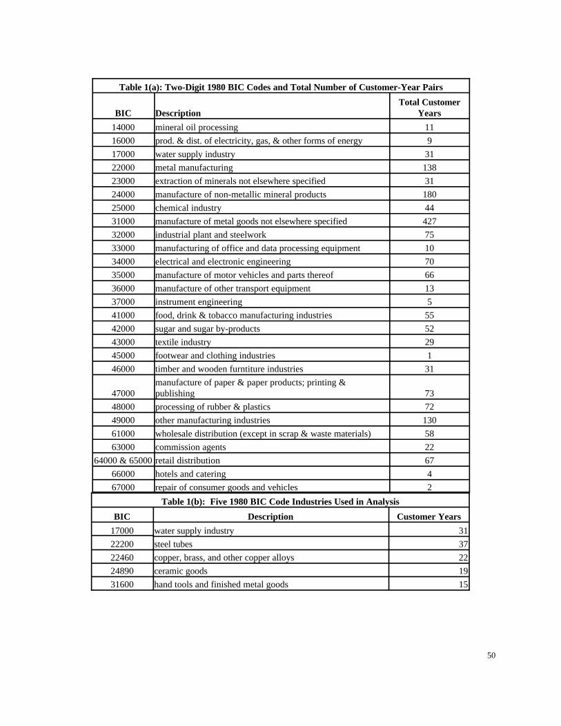
50

Table 1(a): Two-Digit 1980 BIC Codes and Total Number of Customer-Year Pairs

BIC DescriptionTotal Customer

Years

14000 mineral oil processing 11

16000 prod. & dist. of electricity, gas, & other forms of energy 9

17000 water supply industry 31

22000 metal manufacturing 138

23000 extraction of minerals not elsewhere specified 31

24000 manufacture of non-metallic mineral products 180

25000 chemical industry 44

31000 manufacture of metal goods not elsewhere specified 427

32000 industrial plant and steelwork 75

33000 manufacturing of office and data processing equipment 10

34000 electrical and electronic engineering 70

35000 manufacture of motor vehicles and parts thereof 66

36000 manufacture of other transport equipment 13

37000 instrument engineering 5

41000 food, drink & tobacco manufacturing industries 55

42000 sugar and sugar by-products 52

43000 textile industry 29

45000 footwear and clothing industries 1

46000 timber and wooden furntiture industries 31

47000manufacture of paper & paper products; printing &publishing 73

48000 processing of rubber & plastics 72

49000 other manufacturing industries 130

61000 wholesale distribution (except in scrap & waste materials) 58

63000 commission agents 22

64000 & 65000 retail distribution 67

66000 hotels and catering 4

67000 repair of consumer goods and vehicles 2

Table 1(b): Five 1980 BIC Code Industries Used in Analysis

BIC Description Customer Years

17000 water supply industry 31

22200 steel tubes 37

22460 copper, brass, and other copper alloys 22

24890 ceramic goods 19

31600 hand tools and finished metal goods 15

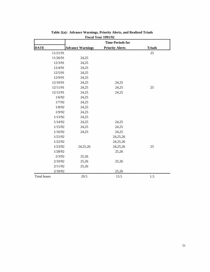
51

Table 2(a): Advance Warnings, Priority Alerts, and Realized TriadsFiscal Year 1991/92

Time Periods for

DATE Advance Warnings Priority Alerts Triads

11/21/91 25

11/26/91 24,25

12/3/91 24,25

12/4/91 24,25

12/5/91 24,25

12/9/91 24,25

12/10/91 24,25 24,25

12/11/91 24,25 24,25 25

12/12/91 24,25 24,25

1/6/92 24,25

1/7/92 24,25

1/8/92 24,25

1/9/92 24,25

1/13/92 24,25

1/14/92 24,25 24,25

1/15/92 24,25 24,25

1/16/92 24,25 24,25

1/21/92 24,25,26

1/22/92 24,25,26

1/23/92 24,25,26 24,25,26 25

1/28/92 25,26

2/3/92 25,26

2/10/92 25,26 25,26

2/11/92 25,26

2/18/92 25,26

Total hours 20.5 13.5 1.5

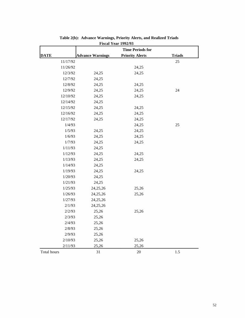
52

Table 2(b): Advance Warnings, Priority Alerts, and Realized TriadsFiscal Year 1992/93

Time Periods for

DATE Advance Warnings Priority Alerts Triads

11/17/92 25

11/26/92 24,25

12/3/92 24,25 24,25

12/7/92 24,25

12/8/92 24,25 24,25

12/9/92 24,25 24,25 24

12/10/92 24,25 24,25

12/14/92 24,25

12/15/92 24,25 24,25

12/16/92 24,25 24,25

12/17/92 24,25 24,25

1/4/93 24,25 25

1/5/93 24,25 24,25

1/6/93 24,25 24,25

1/7/93 24,25 24,25

1/11/93 24,25

1/12/93 24,25 24,25

1/13/93 24,25 24,25

1/14/93 24,25

1/19/93 24,25 24,25

1/20/93 24,25

1/21/93 24,25

1/25/93 24,25,26 25,26

1/26/93 24,25,26 25,26

1/27/93 24,25,26

2/1/93 24,25,26

2/2/93 25,26 25,26

2/3/93 25,26

2/4/93 25,26

2/8/93 25,26

2/9/93 25,26

2/10/93 25,26 25,26

2/11/93 25,26 25,26

Total hours 31 20 1.5

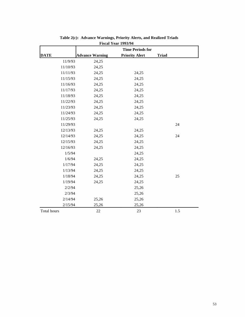
53

Table 2(c): Advance Warnings, Priority Alerts, and Realized TriadsFiscal Year 1993/94

Time Periods for

DATE Advance Warning Priority Alert Triad

11/9/93 24,25

11/10/93 24,25

11/11/93 24,25 24,25

11/15/93 24,25 24,25

11/16/93 24,25 24,25

11/17/93 24,25 24,25

11/18/93 24,25 24,25

11/22/93 24,25 24,25

11/23/93 24,25 24,25

11/24/93 24,25 24,25

11/25/93 24,25 24,25

11/29/93 24

12/13/93 24,25 24,25

12/14/93 24,25 24,25 24

12/15/93 24,25 24,25

12/16/93 24,25 24,25

1/5/94 24,25

1/6/94 24,25 24,25

1/17/94 24,25 24,25

1/13/94 24,25 24,25

1/18/94 24,25 24,25 25

1/19/94 24,25 24,25

2/2/94 25,26

2/3/94 25,26

2/14/94 25,26 25,26

2/15/94 25,26 25,26

Total hours 22 23 1.5

54

Table 2(d): Triad Advance Warnings, Priority Alerts, and Realized TriadsFiscal Year 1994/95

Time Periods for

DATE Advance Warning Priority Alert Triad

11/28/94 24,25

11/29/94 24,25 24,25

12/5/94 24,25 24,25

12/6/94 24,25 24,25

12/7/94 24,25 24,25

12/8/94 24,25 24,25

12/12/94 24,25 24,25

12/13/94 24,25 24,25

12/14/94 24,25 24,25 25

12/15/94 24,25 24,25

12/19/94 24,25 24,25

12/20/94 24,25 24,25

12/21/94 24,25 24,25

12/22/94 24,25 24,25

1/3/95 24,25 24,25

1/4/95 24,25 25

1/10/95 24,25

1/11/95 25 25

1/12/95 25 25

1/18/95 24,25 24,25

1/19/95 24,25 24,25 25

1/25/95 24,25

1/26/95 24,25

1/30/95 25,26

1/31/95 25,26

Total hours 20 21 1.5

55

Table 3

Sample Means and Standard Deviations of Components of PSP

Year Mean Std Dev

SMP 1 19.52 4.10

CC 1 1.29 8.76

UPLIFT 1 1.61 2.31

PSP 1 22.42 12.72

SMP 2 22.64 4.24

CC 2 0.17 1.70

UPLIFT 2 1.39 1.12

PSP 2 24.19 5.75

SMP 3 24.16 6.71

CC 3 0.28 2.97

UPLIFT 3 2.18 1.62

PSP 3 26.62 8.76

SMP 4 20.78 12.28

CC 4 3.22 24.49

UPLIFT 4 2.38 4.53

PSP 4 26.38 35.08

56

Table 4: Coefficients Estimates and Probability Derivatives for Day-Ahead Probability of Triad or Demand Charge Function

Parameter Estimate Standard Error Probability Derivative

Constant -8.682 1.790

Lagged Value of TSL 0.254E-03 0.871E-04 1.0215E-07

Triad Adv. Warning -0.217 0.388 -0.000087

Priority Alert 1.643 0.395 0.00065

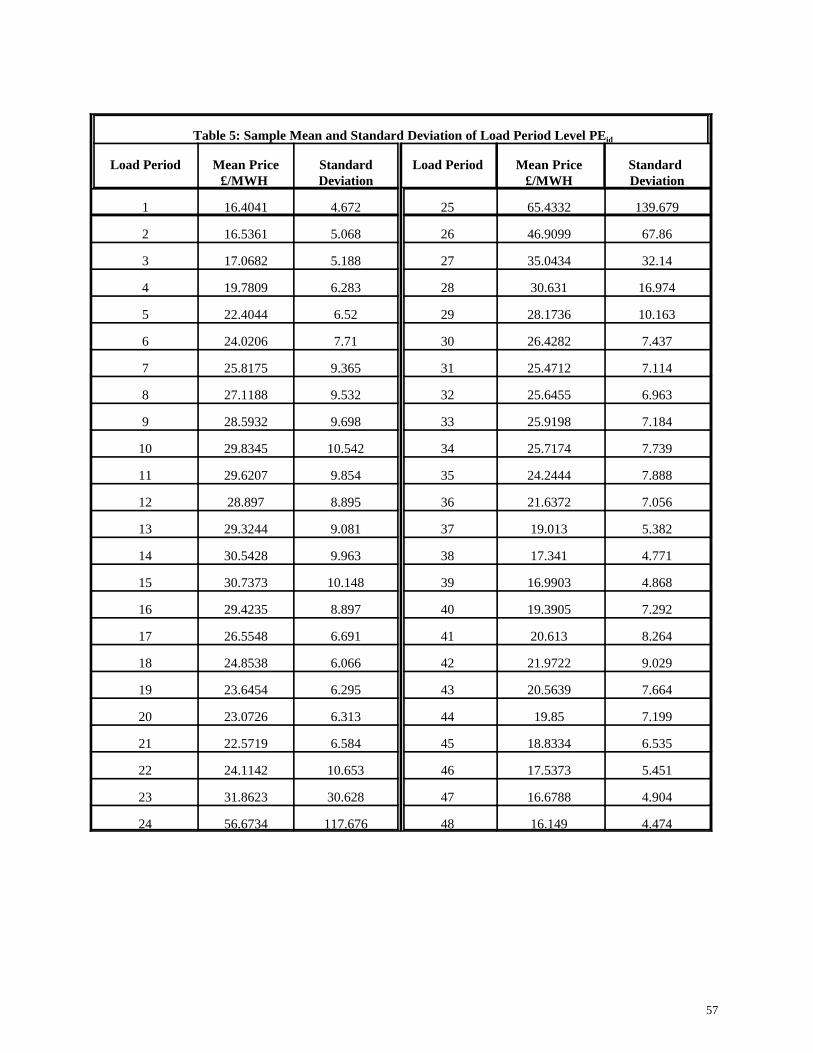
57

Table 5: Sample Mean and Standard Deviation of Load Period Level PEid

Load Period Mean Price£/MWH

StandardDeviation

Load Period Mean Price£/MWH

Standard Deviation

1 16.4041 4.672 25 65.4332 139.679

2 16.5361 5.068 26 46.9099 67.86

3 17.0682 5.188 27 35.0434 32.14

4 19.7809 6.283 28 30.631 16.974

5 22.4044 6.52 29 28.1736 10.163

6 24.0206 7.71 30 26.4282 7.437

7 25.8175 9.365 31 25.4712 7.114

8 27.1188 9.532 32 25.6455 6.963

9 28.5932 9.698 33 25.9198 7.184

10 29.8345 10.542 34 25.7174 7.739

11 29.6207 9.854 35 24.2444 7.888

12 28.897 8.895 36 21.6372 7.056

13 29.3244 9.081 37 19.013 5.382

14 30.5428 9.963 38 17.341 4.771

15 30.7373 10.148 39 16.9903 4.868

16 29.4235 8.897 40 19.3905 7.292

17 26.5548 6.691 41 20.613 8.264

18 24.8538 6.066 42 21.9722 9.029

19 23.6454 6.295 43 20.5639 7.664

20 23.0726 6.313 44 19.85 7.199

21 22.5719 6.584 45 18.8334 6.535

22 24.1142 10.653 46 17.5373 5.451

23 31.8623 30.628 47 16.6788 4.904

24 56.6734 117.676 48 16.149 4.474

58

Table 6: Holiday Dummies yd(j)

Dummy Variable Holidays

j=1 Christmas(days 1 and 2),New Years Day

j=2 Good Friday, Easter Monday

j=3 May Day, Spring Bank

j=4 Late Summer

59

Figure 1: Sample Pool Price Contract Day-Ahead fax

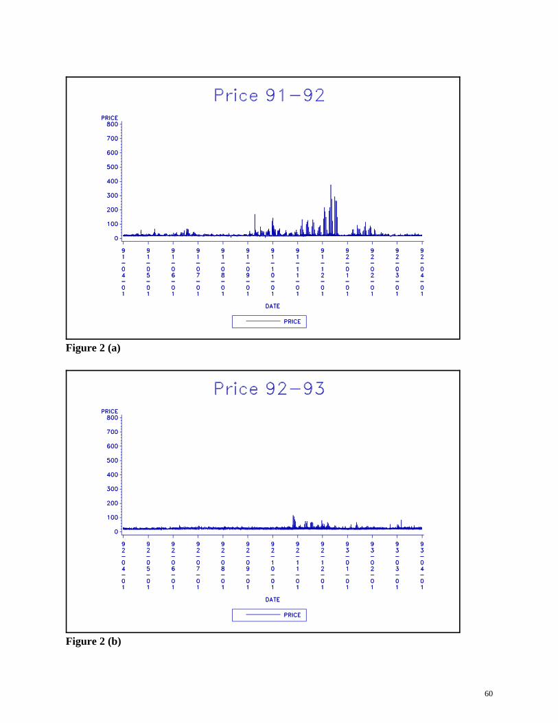
60

Figure 2 (a)

Figure 2 (b)

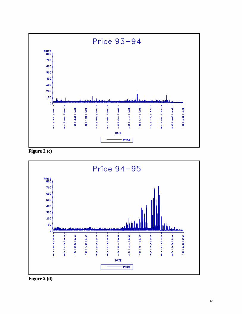
61

Figure 2 (c)

Figure 2 (d)

Figure 2 (c)

Figure 2 (d)

62

Figure 3 (a)

Figure 3 (b)

63

Figure 3 (c)

Figure 3 (d)

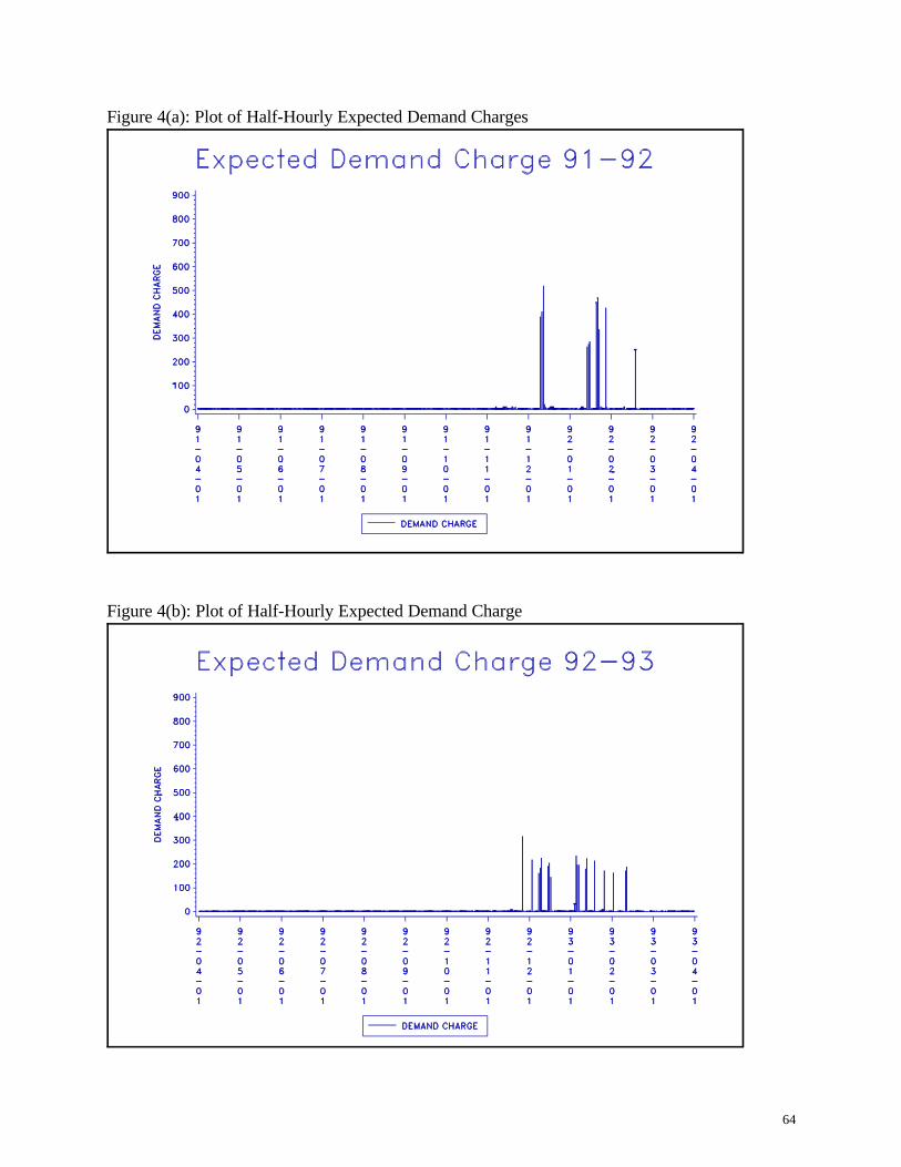
64

Figure 4(a): Plot of Half-Hourly Expected Demand Charges

Figure 4(b): Plot of Half-Hourly Expected Demand Charge

65

Figure 4(c): Plot of Half-Hourly Expected Demand Charge

Figure 4(d): Plot of Half-Hourly Expected Demand Charge

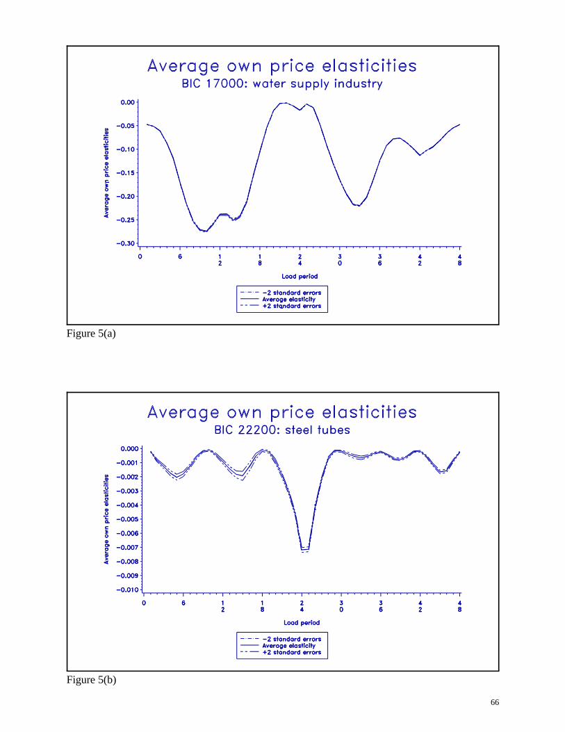
66

Figure 5(a)

Figure 5(b)

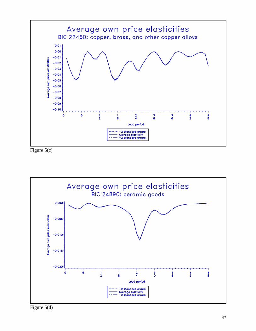
67

Figure 5(c)

Figure 5(d)

68

Figure 5(d)

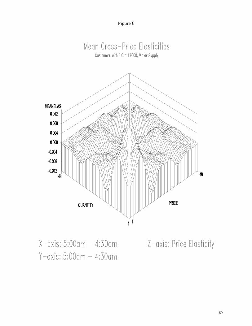
69

Figure 6

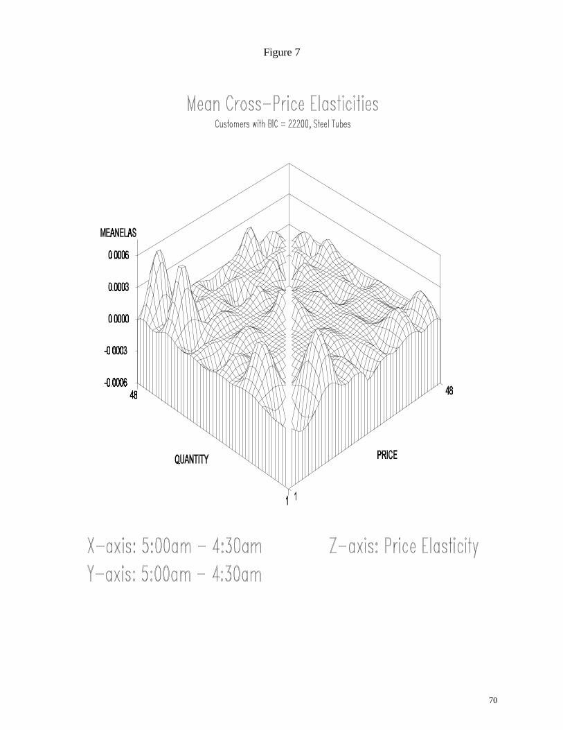
70

Figure 7

71

Figure 8

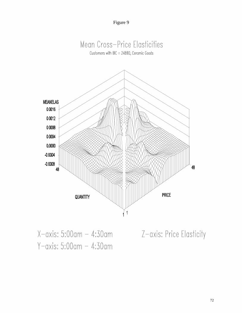
72

Figure 9

73

Figure 10

74

Figure 11

Figure 12