Estimating species tolerance to human perturbation: Expert judgment versus empirical approaches

This article appeared in a journal published by Elsevier. The attachedcopy is furnished to the author for internal non-commercial researchand education use, including for instruction at the authors institution

and sharing with colleagues.

Other uses, including reproduction and distribution, or selling orlicensing copies, or posting to personal, institutional or third party

websites are prohibited.

In most cases authors are permitted to post their version of thearticle (e.g. in Word or Tex form) to their personal website orinstitutional repository. Authors requiring further information

regarding Elsevier’s archiving and manuscript policies areencouraged to visit:

http://www.elsevier.com/copyright

Author's personal copy

Ecological Indicators 11 (2011) 1623–1635

Contents lists available at ScienceDirect

Ecological Indicators

journa l homepage: www.e lsev ier .com/ locate /eco l ind

Estimating species tolerance to human perturbation: Expert judgment versusempirical approaches

Pedro Seguradoa,∗, José Maria Santosa, Didier Pontb, Andreas H. Melcherc, Diego Garcia Jalond,Robert M. Hughese, Maria Teresa Ferreiraa

a Centro de Estudos Florestais, Technical University of Lisbon, Tapada da Ajuda, 1349-017 Lisboa, Portugalb Cemagref, Hydrosystems and Bioprocesses Research Unit (HBAN), Parc de Tourvoie BP44, 92163 Antony Cedex, Francec Institute of Hydrobiology and Aquatic Ecosystem Management, BOKU – University of Natural Resources and Life Sciences, Max Emanuelstr. 17, 1180 Vienna, Austriad Department of Zoology, ETSI Montes, Universidad Politecnica de Madrid, Avenida Ramiro de Maeztu s/n, 28040 Madrid, Spaine Department of Fisheries and Wildlife, Oregon State University, 200 SW 35th Street & Amnis Opes Institute, 2895 SE Glenn, Corvallis, OR 97333, United States

a r t i c l e i n f o

Article history:Received 13 November 2010Received in revised form 23 February 2011Accepted 8 April 2011

Keywords:Ecological indicatorsEnvironmental variabilityMediterranean freshwater fishAnthropogenic pressuresWeighted averagingNiche modelling

a b s t r a c t

Species tolerances are frequently used in multi-metric ecological quality indices, and typically have thestrongest responses to disturbances. Usually the tolerances of many species are based on expert judg-ment, with little support from empirical ecological or physiological data. This is particularly true for fish ofMediterranean-type rivers, in which there are many basin-endemic taxa with little information on basiclife history traits. In addition, the apparent tolerance of native Mediterranean freshwater fish speciesto naturally harsh environments and their short-term resilience may mask responses to man-madepressures. Consequently, we evaluated different statistical techniques and procedures for quantifyingMediterranean lotic fish tolerances and compared expert judgment of species tolerances with empiri-cally determined tolerance values. We used eight alternative approaches to compute fish tolerance valuesfor the Mediterranean basins of SW Europe. Three types of approaches were used: (1) those based onthe concept of niche breadth along an environment/pressure gradient (five models); (2) those based ondeviations from expected values at disturbed sites as predicted by statistical models describing relation-ships between species and environmental variables (generalized linear modelling (GLM) and generalizedadditive modelling (GAM), two models); and (3) one model based on the relatively independent contri-butions of pressure variables to the data variation explained by statistical models. Tolerance estimatesbased on the used/available pressure gradient and the average general pressure value had the highestmean correlations with the expert judgment classification (mean r = 0.4) and with the other approaches(mean r of 0.48 and 0.46, respectively). The high degree of uncertainty in tolerance estimates should beaccounted for when applying them in ecological assessments. Results also highlights the need for betterdesigned research to separate effects of natural and disturbance gradients on species occurrences anddensities.

© 2011 Elsevier Ltd. All rights reserved.

1. Introduction

Species that are considered generally sensitive or tolerant tohuman disturbances are commonly used as indicators of healthyecosystems or ecosystem deterioration, respectively. Deteriorationor disturbance of terrestrial ecosystems associated with devegeta-tion or economic development has been linked to losses of sensitivespecies or increases in the proportions of tolerant, weedy, or gen-eralist species (e.g. Stolte and Mangis, 1992; Bryce et al., 2002).

∗ Corresponding author at: Centro de Estudos Florestais, Instituto Superior deAgronomia, Tapada da Ajuda P-1349-017 Lisboa, Portugal. Tel.: +351 21 365 3380;fax: +351 21 365 31 95.

E-mail address: [email protected] (P. Segurado).

Likewise, in aquatic ecosystems, eutrophication, warming and sed-imentation are associated with losses of sensitive or intolerantspecies and increases in tolerant species (Hughes and Noss, 1992;Davies and Jackson, 2006). Often the tolerant species are invasivealien species. Some sensitive species that were once widespreadare now endangered, threatened, or vulnerable.

The idea of using species tolerances in biological assessmentsof aquatic ecosystem condition began with Kolkwitz and Marsson(1909). Later, Chutter (1972) and Hilsenhoff (1977) proposed tol-erance indices based on the responses of various taxa to organicpollution or low dissolved oxygen. But the taxa tolerance rank-ings in those publications were based on qualitative judgments.Most subsequent tolerance rankings for aquatic taxa also have beenbased on professional judgments and/or empirical literature fromother regions (e.g. Plafkin et al., 1989; Barbour et al., 1999).

1470-160X/$ – see front matter © 2011 Elsevier Ltd. All rights reserved.doi:10.1016/j.ecolind.2011.04.006

Author's personal copy

1624 P. Segurado et al. / Ecological Indicators 11 (2011) 1623–1635

Rankings of fish species tolerances have been determined graph-ically or through use of simple mathematical analyses (Whittierand Hughes, 1998; Pirhalla, 2004). Although not accounting fornatural variability, these methods are easily implemented and visu-ally understandable. With increased computing power and largeregional and national data sets collected via standard methods,aquatic ecologists have recently been able to quantitatively evalu-ate how aquatic taxa respond along a variety of stressor gradients.For example, weighted averaging (WA) has been employed todetermine diatom species tolerances in northeastern USA lakes(Dixit et al., 1999), fish species tolerances in USA streams (Meadorand Carlisle, 2007) and western USA streams and rivers (Whittieret al., 2007a), and macroinvertebrate taxon tolerances in westernUSA streams and rivers (Whittier and Van Sickle, 2010). None ofthese studies used methods that explicitly controlled for naturalvariability.

Yuan (2004) indicated that incorporating natural covariatesimproved many of the generalized additive modelling (GAM)tolerance models developed for Mid-Atlantic Highlands macroin-vertebrate genera. Yuan (2006) reviewed four statistical methodsfor estimating macroinvertebrate tolerance values from fielddata: (1) cumulative percentiles, (2) WA, (3) parametric regres-sion (GLM, generalized linear modelling), and (4) non-parametricregression (GAM). He found that all four approaches producedhighly correlated (0.84–0.98) tolerance values. Yuan (2006) recom-mended including environmental correlates in regression-basedapproaches to control for natural gradients, and being cognizant ofthe range of environmental conditions from which taxon tolerancesare derived.

More recently, Hermoso et al. (2009) used principal componentanalysis (PCA) to derive a synthetic pressure gradient (2nd PCAaxis) that was presumed to be independent from natural variability,and included site-, reach- and basin-scale stressors and pressures.Their index of species sensitivity was based on the over- and under-use of both extremes of the perturbation gradient through use ofa chi-square test. The main limitation of their approach is that itis difficult to extract a perturbation gradient that is sufficientlyindependent from natural variability.

The biological focus of the European Water Framework Direc-tive and the U.S. Clean Water Act have led to the developmentof indices of biological integrity for assessing water body qualityat multistate regional, national, and continental scales in Europe(Oberdorff et al., 2002; Pont et al., 2006, 2007; Melcher et al.,2007; Schmutz et al., 2007) and the U.S. (Whittier et al., 2007b;Paulsen et al., 2008; Pont et al., 2009a). Each of these indicesincludes one or more metrics for measuring tolerant or sensi-tive taxa or individuals. Although exceptions exist (e.g. Meadorand Carlisle, 2007; Whittier et al., 2007a; Hermoso et al., 2009;Whittier and Van Sickle, 2010), there are no empirical toleranceclassifications for most aquatic species. This is particularly truefor lotic fish species endemic to Mediterranean basins. Toler-ance classifications for such species are hindered by the natural(but seasonally predictable) harshness of Mediterranean streams,which experience naturally wide temperature and flow extremes(Gasith and Resh, 1999). Therefore, quantifying species tolerancein such ecosystems is extremely important to improve knowledgeof species ecology and more accurate assessment of assemblagecondition.

The objectives in this study were to: (1) quantify the tol-erances of Mediterranean freshwater fish species to generalhuman-induced pressures; (2) assess and compare differentquantitative approaches for species tolerance quantification; (3)test alternative methods for controlling for natural environ-mental gradients; and (4) assess the extent to which expertjudgment qualitative classifications are supported by empiricaldata.

2. Materials and methods

2.1. Study area

The study area included 39 major basins from Iberia, Italy, andFrance (Fig. 1). For Italy and France, we considered only sites withinthe Mediterranean geographic boundary (for Italy only Alpine siteswere not considered). All sites from Iberia were considered in theanalyses since it functions as a biogeographical unit (Reyjol et al.,2007). Because one objective was to explore methods to controlfor natural environmental variability on tolerance estimates, wesought to encompass as wide an ecological gradient as possiblefor each species. To determine the Mediterranean boundary, weused a total annual precipitation (TAP) threshold of 1200 mm andthe summer ombrothermic index (Ios4; Rivas-Martínez and Loidi-Arregui, 1999), which measured hydrological stress from May toAugust.

2.2. Biological data

Our fish data were obtained via fish surveys conductedby several academic institutions and environmental agencies.The dataset included presence/absence data at 5011 sitessampled from 1981 to 2007 (see EFI+ project website: http://efi-plus.boku.ac.at/download.htm, 18 October 2010; Fig. 2). Sites weresampled by electrofishing during low flow periods employing stan-dard European methods (CEN, 2003), mostly by wading (97%). Foreach species, analyses were restricted to sites located within theirpotential geographical range (i.e. areas where the species maypotentially occur through dispersion). We included only sites withfished areas greater than 100 m2 and more than 30 individualscaught to minimize the risk of false absences. No such data screen-ing was used for species’ presence data. Only those species thatwere present in at least five sites were considered in subsequentanalyses.

2.3. Environmental and pressure variables

Twelve variables describing the natural environmental gradi-ent were considered. These variables comprised three climatic(mean total annual precipitation on the catchment, local mean Julytemperature, local difference between mean January and July tem-peratures), three topographical (mean catchment altitude, localaltitude, river slope), one geological (natural substrate) and fivevariables directly or indirectly related to river geomorphology (geo-morphologic river type, valley form, floodplain extent, distance tosource, catchment area). The climatic, topographical and geologi-cal variables were derived from the CCM2 European River Network(Vogt et al., 2007). Qualitative information on geomorphologicriver type, floodplain extent, valley form and natural substrate wasrecorded during field work or through expert evaluation. Whennecessary, these data were supplemented with visual analyses fromGoogle Earth.

We used Smith–Hill ordination (Hill and Smith, 1976) to sum-marize geomorphological information that included mixed-typevariables (quantitative, factor and ordered) (factor loadings areshown in Appendix A). We ran the ordination using the Ade4 pack-age (Thioulouse et al., 1997) for R version 7.0.1 (R DevelopmentCore Team, 2007).

For each site, we also assessed human-induced pressuresdescribed by 17 variables based on site measurements, expertjudgment, and Google Earth. Pressures acting on river connec-tivity, hydrology, morphology and water quality were considered(Appendix B).

Author's personal copy

P. Segurado et al. / Ecological Indicators 11 (2011) 1623–1635 1625

Fig. 1. Study area location and major river basins.

Fig. 2. Locations of sample sites (black dots are least-disturbed sites used for model calibrations).

Author's personal copy

1626 P. Segurado et al. / Ecological Indicators 11 (2011) 1623–1635

2.4. Classification of species tolerance based on expert judgment

Qualitative classification of species tolerances were providedby 13 researchers from 12 European countries (Appendix C), andconducted under the EFI+ project (http://efi-plus.boku.ac.at). Theexpert judgment classification was based on the Delphi method,which is a systematic, iterative, and interactive decision-aiding tool(e.g. Rowe and Wright, 1999). When a consensus among expertswas not reached, the final decisions about the classifications weredetermined from the mean or mode of classification and the liter-ature.

Each species was classified according to its tolerance to physi-cal habitat degradation and to general water quality degradation.For each kind of tolerance, three levels were considered: tolerant,intermediate and intolerant. Species were classified as intolerantor tolerant if they were considered as, respectively, intolerant ortolerant at least for one tolerance guild. Intermediate species werethose that fitted neither the intolerant nor the tolerant classes.

2.5. Statistical analyses

The quantification of fish tolerance values was based on threealternative kinds of approaches: (1) concepts of niche breathand niche position along an environment/pressure gradient; (2)deviations from expected occurrences at disturbed sites basedon statistical models relating species to environmental variables;and (3) partitioning techniques estimating the independent con-tribution of pressure variables on statistical models of speciesdistributions.

A total of eight tolerance values, based on the differentapproaches and using different procedures, were computed. Forcomparison purposes, all tolerance values estimated with the dif-ferent approaches were rescaled to vary between 0 (intolerant) and1 (tolerant). All statistical analyses were performed through use ofR software version 2.7.1 (R Development Core Team, 2007).

2.5.1. Approach 1: tolerance values based on the concepts ofniche breath and niche position

As a first approach, the niche breadth of species along the mainenvironmental gradient was estimated. This measure was assumedto be a surrogate of species tolerance to human-induced pressures,based on the hypothesis that generalist species are more tolerantto pressures than specialist species (the specialization-disturbancehypothesis; Vázquez and Simberloff, 2002). The main environmen-tal gradient was based on the scores of the first and second axes ofa PCA calculated from the available set of environmental variables.Niche breath (NB) was computed as the mean standard deviationof the scores of the two first PCA axes at species presence sitesweighted by their respective eigenvalues (2.69 and 1.68, respec-tively).

In a second approach, WA was used to calculate tolerance val-ues along a general pressure gradient. The species optimum alongthe environmental gradient was obtained by taking the averageof the values of the environmental variables (xi) weighted byspecies absolute abundances (yik), at sites where the species waspresent (Jongman et al., 1995). Because calculations were basedon presence–absence data, the weighted averages were the aver-age general pressure values at sites where species were present.Optima and tolerances were expressed as follows:

Optimum u =∑n

i=1yikxi∑ni=1yik

(1)

Tolerance t =

√∑ni=1yik(xi − u)2∑n

i=1yik

(2)

We considered the upper tolerance (u + t) value as an estimatorof species tolerance to pressures.

A third niche-based approach compared used versus avail-able pressure gradients within species potential ranges (UA). Thisapproach assumed that species tolerance values would be (1)proportional to the upper limit of species occurrences along thepressure gradient, (2) inversely proportional to the differencebetween the upper limit of available and used pressure gradient,and (3) proportional to the difference between the lower limit ofthe used and available pressure gradients. The resulting tolerancevalue was based on the mean value of those three parameters,after rescaling each from 0 to 1, using the difference between eachvalue and the minimum value divided by the difference betweenthe maximum and the minimum values. Upper and lower limitsfor both the available and used pressure gradients were defined,respectively, as the 2.5 and 97.5 percentiles of the pressure gradi-ent.

Two alternative procedures were used to extract the generalperturbation gradient used with the WA and UA approaches:multiple correspondence analysis (MCA) and partial principal com-ponent analysis (PCAp). To compute PCAp, each pressure variablewas first regressed against the environmental variables and theresulting residuals were then used in the PCA (ter Braak, 1995).The resulting axis represents the pressure gradient that is inde-pendent of environmental variability. Therefore, two alternativetolerance values were computed for the WA and UA approachesby considering these two general pressure gradients. Hence, a totalof five tolerance values based on the concepts of niche breath andniche position were computed (NB, WA MCA, WA PCAp, UA MCA,UA PCAp).

2.5.2. Approach 2: tolerance values based on deviations fromexpected species occurrences

The response of species to human-induced pressures was alsoquantified through use of predictive model residuals (Oberdorffet al., 2002; Pont et al., 2006). Statistical models relating eachspecies presence–absence to the set of environmental predictorswere first adjusted using a calibration dataset of least-disturbedsites. The calibration model was then used to predict species pres-ence/absence for the remaining sites. The difference between theobserved and the predicted metric values (residuals) was assumedto be proportional to some kind of human-induced pressure. In thisway, it would be possible to isolate the effect of human-induceddisturbances from that of natural environmental variability.

Both generalized linear modelling (McCullagh and Nelder, 1989)and generalized additive modelling (Hastie and Tibshirani, 1990),assuming a binomial distribution of errors and a logit function,were used to determine the relationships between each speciesand the environmental variables. We used a stepwise Akaike Infor-mation Criterion (Venables and Ripley, 1997) to select variablesfor inclusion in models. Redundant variables (Pearson r > 0.7) wererestricted from the same model. Many species had a limited numberof sites available for model development because only sites withinthe geographical range of each species were used for each speciesmodel and the respective projections. Only those species with aminimum of 25 sites, including at least 10 absence and 10 presencesites, were considered to yield potentially acceptable models.

The selection of least-disturbed sites used in model calibrationfollowed the criteria used in the EU-project EFI+ (http://efi-plus.boku.ac.at), with two adaptations for Mediterranean rivers.The intermediate disturbance classes for both eutrophication andriparian vegetation degradation were included in the calibrationset. A total of 748 sites (Fig. 2) were available to calibrate modelsof metric response to environmental variability.

We then employed a residual standardization procedure basedon Pont et al. (2006, 2007). The last step of the approach was to

Author's personal copy

P. Segurado et al. / Ecological Indicators 11 (2011) 1623–1635 1627

Table 1Fish species with occurrence ≥5, number of sites included within the geographical range of each species, and total number of occurrences.

Species Common names Number of sites Number of occurrences

Salmo trutta fario Brown trout 1979 1231Anguilla anguilla European Eel 2053 630Luciobarbus bocageia Iberian barbel 855 439Squalius carolitertiia Northern Iberian chub 909 355Pseudochondrostoma duriensea Northern straight-mouth nase 767 336Phoxinus bigerrib Pyrenean minnow 1023 312Squalius alburnoidesa Calandino 854 301Pseudochondrostoma polylepisa Iberian straight-mouth nase 833 271Squalius pyrenaicusa Southern Iberian chub 790 261Lepomis gibbosusd Pumpkinseed 1601 259Gobio lozanoib Pyrenean gudgeon 1607 257Cobitis paludicaa Southern Iberian spined-loach 1337 225Achondrostoma arcasiia Bermejuela 1167 171Achondrostoma oligolepisa Ruivaco 748 151Barbatula sp. Stone loach 824 146Parachondrostoma miegiia Ebro nase 817 129Luciobarbus graellsiia Ebro barbel 815 121Gambusia holbrookid Eastern mosquitofish 1526 100Micropterus salmoidesd Largemouth bass 1749 100Cyprinus carpiod Common carp 1592 94Carassius auratusd Goldfish 1403 92Salmo salar Atlantic salmon 782 81Luciobarbus comizoa Iberian long-snout barbel 397 80Luciobarbus sclateria Southern Iberian barbel 227 79Iberochondrostoma lemmingiia Iberian arched-mouth nase 698 48Luciobarbus microcephalus Iberian small-head barbel 106 44Cobitis calderonia Northern Iberian spined-loach 862 44Pseudochondrostoma willkommiia Southern straight-mouth nase 136 43Alburnus alburnus Bleak 651 37Gasterosteus gymnurus Three-spined stickleback 1293 37Leuciscus cephalus Chub 60 37Australoheros facetusd Chameleon cichlid 393 36Squalius aradensisa Arade chub 56 34Barbus tyberinusc Barbo tiberino 51 33Rutilus rubilioc Rovella 51 33Leuciscus souffia Vairone 53 32Oncorhynchus mykissd Rainbow trout 1656 31Platichthys flesus European flounder 868 29Iberochondrostoma lusitanicuma Portuguese arched-mouth nase 334 28Petromyzon marinus Sea lamprey 1285 28Chelon labrosus Thicklip grey mullet 628 27Leuciscus lucumonisc Cavedano etrusco 45 26Padogobius nigricansc Arno goby 45 24Atherina boyeri Big-scale sand smelt 1092 19Protochondrostoma genei Lasca 45 19Liza ramada Thinlip grey mullet 977 19Iberochondrostoma almacaia Southwestern arched-mouth nase 45 18Lampetra planeri European brook lamprey 888 17Barbus barbus Barbel 54 14Barbus haasia Iberian redfin barbel 186 13Salaria fluviatilis Freshwater blenny 299 13Gobio gobio Gudgeon 59 12Lampetra fluviatilis River lamprey 300 10Pseudorasbora parvad Stone moroko 220 9Ameiurus melasd Black bullhead 622 8Mugil cephalus Flathead grey mullet 721 8Cobitis taenia Spined loach 53 7Padogobius martensii Padanian goby 45 6Rutilus rutilus Roach 167 6Anaecypris hispanicaa Jarabugo 106 5

a Species endemic to the Iberian Peninsula.b Species endemic to the Iberian Peninsula and southwestern France.c Species endemic to the Italian Peninsula.d Alien species.

compute a value that could be used as a surrogate of species tol-erance to the general perturbation gradient. To get a simple butrobust measure of the decrease of residual values at disturbed sites(i.e. species occur less often than predicted by the model) the firstquartile of the residuals of the calibration set was subtracted fromthe third quartile of the non-calibration set. Because residuals werepreviously standardized and transformed, it is possible to compare

the resulting values between species. These analyses produced twoestimates of species tolerances (GLM and GAM).

2.5.3. Approach 3: tolerance values based on variationpartitioning techniques

In this approach we assumed that tolerance to pressure wasinversely proportional to the percentage of variation in species data

Author's personal copy

1628 P. Segurado et al. / Ecological Indicators 11 (2011) 1623–1635

Table 2Tolerance classification based on expert judgment and the estimated species’ tolerance values with each approach.

Species Tolerance classification NB WA MCA WA PCAp UA MCA UA PCAp HPART GLM GAM

A. arcasii Intolerant 0.79 0.23 0.46 0.05 0.37 0.99 0.13 0.07B. barbus Intolerant 0.29 0.52 0.29 0.58 0.45 0.97B. haasi Intolerant 0.90 0.26 0.33 0.18 0.28 0.97B. tyberinus Intolerant 0.26 0.10 0.10 0.33 0.37 0.95C. calderoni Intolerant 0.67 0.38 0.44 0.26 0.46 0.94I. almacai Intolerant 0.00 0.00 0.14 0.14 0.30 0.87L. fluviatilis Intolerant 0.02 0.68 0.60 0.46 0.47 0.77L. planeri Intolerant 0.60 0.40 0.37 0.24 0.17 0.67L. souffia Intolerant 0.23 0.24 0.28 0.36 0.59 1.00P. genei Intolerant 0.22 0.04 0.00 0.15 0.12 0.89 0.00 0.27P. miegii Intolerant 0.82 0.69 1.00 0.65 1.00 0.56 0.10 0.02P. bigerri Intolerant 0.68 0.42 0.76 0.52 0.82 0.81 0.93 0.82S. salar Intolerant 0.13 0.19 0.36 0.21 0.21 0.93 0.05 0.01S. trutta fario Intolerant 0.80 0.09 0.40 0.19 0.42 0.74 0.01 0.00A. hispanica Intermediate 0.37 0.11 0.03 0.00 0.00 0.82A. boyeri Intermediate 0.92 0.83 0.43 0.65 0.36 0.94B. quignardi Intermediate 0.82 0.60 0.94 0.53 0.92 0.79 0.34 0.33C. paludica Intermediate 0.84 0.53 0.50 0.60 0.56 0.97 0.52 0.42C. taenia Intermediate 0.14 0.31 0.15 0.16 0.16 0.94G. gymnurus Intermediate 0.70 0.36 0.60 0.35 0.75 0.99 0.03 0.00G. gobio Intermediate 0.35 0.55 0.45 0.56 0.51 0.00G. lozanoi Intermediate 0.83 0.51 0.55 0.55 0.53 0.90 0.04 0.01I. lemmingii Intermediate 0.54 0.28 0.30 0.10 0.19 0.81I. lusitanicum Intermediate 0.38 0.60 0.86 0.43 0.87 0.96L. bocagei Intermediate 0.88 0.56 0.56 0.65 0.55 0.82 0.76 0.69L. cephalus Intermediate 0.30 0.24 0.12 0.46 0.36 0.94 0.00 0.98L. comizo Intermediate 0.63 0.54 0.44 0.25 0.38 0.99L. graellsii Intermediate 0.84 0.70 0.94 0.64 0.93 0.59L. microcephalus Intermediate 0.50 0.52 0.45 0.47 0.40 0.79O. mykiss Intermediate 0.64 0.27 0.48 0.49 0.94 0.98 0.04 0.00P. martensii Intermediate 0.35 0.29 0.22 0.26 0.26 0.92P. nigricans Intermediate 0.30 0.08 0.07 0.29 0.25 0.96 0.72 1.00P. marinus Intermediate 0.39 0.44 0.26 0.56 0.09 0.89P. flesus Intermediate 0.19 0.81 1.00 0.75 0.92 0.87P. duriense Intermediate 0.56 0.22 0.47 0.39 0.48 0.82 0.39 0.63P. polylepis Intermediate 0.83 0.56 0.52 0.55 0.45 0.85 1.00 0.97P. willkommii Intermediate 0.63 0.51 0.31 0.32 0.40 0.94R. rubilio Intermediate 0.28 0.09 0.07 0.30 0.37 0.97 0.00 0.14S. fluviatilis Intermediate 0.76 0.57 0.32 0.53 0.09 0.91S. aradensis Intermediate 0.07 0.01 0.13 0.13 0.32 0.91S. carolitertii Intermediate 0.79 0.30 0.53 0.37 0.53 0.84 0.53 0.41S. pyrenaicus Intermediate 0.64 0.41 0.42 0.48 0.41 0.82 0.43 0.66A. oligolepis Tolerant 0.35 0.47 0.54 0.36 0.43 0.96A. alburnus Tolerant 0.38 0.49 0.38 0.45 0.56 0.96A. melas Tolerant 0.69 0.54 0.25 0.55 0.44 0.97A. anguilla Tolerant 0.91 0.45 0.60 0.54 0.75 0.99 0.49 0.38A. facetus Tolerant 0.62 0.55 0.39 0.50 0.17 0.95B. sclateri Tolerant 0.61 0.13 0.07 0.26 0.09 0.59 0.07 0.05C. auratus Tolerant 0.88 0.84 0.94 0.79 0.85 0.65C. labrosus Tolerant 0.66 0.71 0.91 0.62 0.72 0.88C. carpio Tolerant 0.71 0.82 0.64 0.74 0.67 0.79G. holbrooki Tolerant 0.76 0.78 0.59 0.77 0.74 0.90L. gibbosus Tolerant 0.84 0.69 0.53 0.84 0.52 0.87L. lucumonis Tolerant 0.24 0.03 0.09 0.16 0.24 0.92 0.00 0.12L. ramada Tolerant 0.81 1.00 0.85 1.00 0.88 0.87M. salmoides Tolerant 0.82 0.77 0.53 0.91 0.50 0.86M. cephalus Tolerant 1.00 0.90 0.99 0.98 0.88 0.90P. parva Tolerant 0.30 0.24 0.11 0.15 0.18 1.00R. rutilus Tolerant 0.33 0.52 0.43 0.54 0.39 0.96S. alburnoides Tolerant 0.81 0.47 0.47 0.50 0.51 0.97 0.38 0.47

NB: niche breath approach; WA MCA: weighted averaging with MCA; WA PCAp: weighted averaging with partial PCA; UA MCA: used versus available with MCA; UA PCAp:used versus available with partial PCA; HPART: hierarchical partitioning; GLM: residual approach using GLM; GAM: residual approach using GAM.

explained exclusively by the general pressure gradient. Variationpartitioning methods aid estimating the independent and sharedcomponents of variation in species data. Here, a hierarchical par-titioning (HPART) approach was used to quantify the independent(i.e. controlling for natural environmental co-variability) contribu-tion of the general pressure gradient on the occurrence of eachspecies.

Hierarchical partitioning involved the computation of theincrease in the fit of models with a particular predictor compared

to the equivalent model without that variable, and averaging theimprovement in the fit across all possible models (i.e. consid-ering all possible variable combinations) with that predictor. Asa result, for each independent variable, hierarchical partitioningprovided an estimate of the independent and shared contribu-tion with all remaining variables (Chevan and Sutherland, 1991).This approach was based on logistic regression models using eachspecies presence/absence as the response variable and the avail-able environmental variables and general pressure index derived

Author's personal copy

P. Segurado et al. / Ecological Indicators 11 (2011) 1623–1635 1629

Table 3Pearson correlation matrix of estimated tolerance values between pairs of the methods used. The mean correlation coefficient, expressing the consistency of each methodwith the remaining methods, and the correlation with tolerance values obtained by Hermoso et al. (2009) are also shown.

NB WA MCA WA PCAp UA MCA UA PCAp HPART GLM GAM

NBWA MCA 0.52***

WA PCAp 0.53*** 0.78***

UA MCA 0.50*** 0.87*** 0.69***

UA PCAp 0.42** 0.60*** 0.86*** 0.65***

HPART −0.08 −0.18 −0.23 −0.17 −0.14GLM 0.39 0.45* 0.32 0.49* 0.19 −0.02GAM −0.03 0.17 −0.07 0.35 −0.08 0.10 0.75***

Mean correlation 0.32 0.46 0.41 0.48 0.36 −0.10 0.37 0.17Avail/useda 0.57 0.62 0.84** 0.55 0.62 0.40 – –

a Hermoso et al. (2009).* P < 0.05.

** P < 0.01.*** P < 0.001

from the first axis of a MCA, as predictor variables. Only the inde-pendent contribution of the general pressure index was retained,as an inverse measure of species tolerance.

2.5.4. Evaluation of methodsThe consensus among methods in the tolerance estimates

was assessed using a Pearson correlation matrix. Methods basedon residuals were compared with the remaining methods usingonly the 23 species that were common to all the approaches.The tolerance estimates were also compared with the tolerancevalues from an independent study that employed available-used chi-squared analysis (Hermoso et al., 2009). The Hermosoet al. (2009) study was undertaken in the Guadiana RiverBasin, South-Western Iberian Peninsula, and used 10 species incommon with our study (Anaecypris hispanica, Cobitis paludica,Iberocypris alburnoides, Iberochondrostoma lemmingii, Luciobarbuscomizo, Luciobarbus microcephalus, Luciobarbus sclateri, Pseudo-chondrostoma willkommii, Salaria fluviatilis and Squalius pyrenaicus).

We assessed the ability of the empirical tolerance values to dis-criminate the three tolerance classes through use of the SomersDxy rank correlation, which is an asymmetrical measure of asso-ciation (Harrell, 2001). We used the Hmisc library for R (Harrell,2001) to compute Somers Dxy values and their respective standarddeviations.

3. Results

Of the 103 species in the database, 60 occurred in at least fivesites (Table 1). Only 23 occurred frequently enough at calibrationsites to be used in predictive modelling. Of the 60 species, 21 areendemic to Iberia, two are endemic to both Iberia and SouthernFrance, four are endemic to Italy, and nine are alien species.

The species most frequently quantified as least tolerant bythe different empirical approaches were A. hispanica and Ibero-chondrostoma almacai, whereas Liza ramada was most consistentlyquantified as most tolerant (Table 2). Among the 10 species with thelowest mean tolerance values across different methods, only threewere classified as intolerant by experts (Protochondrostoma genei, I.almacai and Salmo salar), four as intermediate (A. hispanica, Squal-ius aradensis, Cobitis taenia and Padogobius nigricans), and three astolerant (Leuciscus lucumonis, L. sclateri and Pseudorasbora parva).Among the 10 species with the highest mean tolerance values,six were classified as tolerant (Mugil cephalus, L. ramada, Caras-sius auratus, Gambusia holbrooki, Chelon labrosus and Micropterussalmoides), three as intermediate (Luciobarbus graellsii, B. quignar-dia and Platichthys flesus) and one as intolerant (Parachondrostomamiegii). Five alien species were among the 12 species with the high-

est mean tolerance values: C. auratus, G. holbrooki, M. salmoides,Cyprinus carpio and Lepomis gibbosus.

Among the different quantitative approaches to estimatespecies tolerance values, those based on the used/available pres-sure gradient (UA MCA) and the average general pressure value(WA MCA) had the highest mean correlations with the results of theother approaches (mean r of 0.48 and 0.46, respectively; Table 3).The method based on the used/available partial pressure gradient(UA PCAp) had the highest mean correlation with other methodsthat accounted for natural co-variability (mean r = 0.41). Tolerancevalues based on hierarchical partitioning and GAM approacheswere the least correlated with the remaining approaches (meanr of −0.10 and 0.17, respectively). The highest correlation (r = 0.87)was between UA MCA and WA MCA methods. Comparison of tol-erance estimates with those from Hermoso et al. (2009) showedconsiderable agreement between estimates (Table 3), with Pear-son correlation coefficients ranging from 0.40 (HPART) to 0.84(WA PCAp).

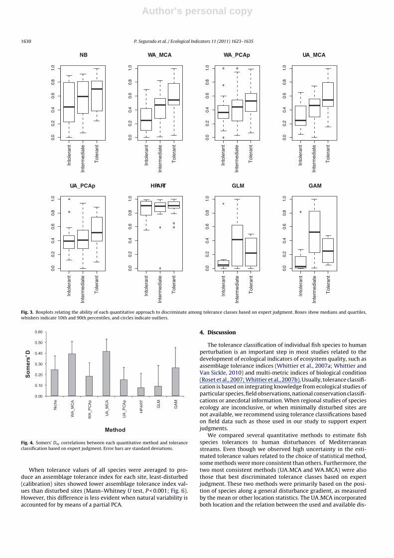
According to Somers Dxy values, UA MCA and WA MCA best dis-criminated the three expert-judgment tolerance classes, followedby NB and GAM-based residual approaches (Figs. 3 and 4). Whennatural environmental variability was accounted for in the gen-eral disturbance gradient by means of a partial PCA (WA PCApand UA PCAp), higher tolerance values were obtained for speciesclassified as intolerant, and slightly lower tolerance values wereobtained for species classified as tolerant. These methods were notable to discriminate between species classified as intolerant andintermediate. In general, methods accounting for natural variabil-ity provided less consistent results (Fig. 4). Among the methods thataccounted for natural environmental variability, the GAM showedthe strongest relationship with the qualitative tolerance classifi-cation, although this method yielded higher tolerance values tospecies classified as intermediate than to species classified as tol-erant. The HPART- and the GLM-based residual approaches hadthe lowest power to discriminate the expert-judgment toleranceclasses.

The plot of the ‘used’ and ‘available’ pressure gradient for eachspecies (Fig. 5) shows that among the 10 more tolerant speciesaccording to the UA MCA method, nine are either diadromous(L. ramada, M. cephalus, P. flesus, Atherina boyeri) or alien species(M. salmoides, L. gibbosus, C. auratus, G. holbrooki, C. carpio). Thesespecies tend to occupy the most disturbed sites along the ‘available’general pressure gradient and to be absent from the less disturbedsites (Fig. 5). Among the 10 most intolerant species, six are Iberianendemics (A. hispanica, Achondrostoma arcasii, I. lemingii, S. araden-sis, I. almacai, B. haasi). These species tend to be absent from themore disturbed sites along the ‘available’ general pressure gradient(Fig. 5).

Author's personal copy

1630 P. Segurado et al. / Ecological Indicators 11 (2011) 1623–1635

Into

lera

nt

Tole

rant

0.0

0.2

0.4

0.6

0.8

1.0

NB

0.0

0.2

0.4

0.6

0.8

1.0

WA_MCA

0.0

0.2

0.4

0.6

0.8

1.0

WA_PCAp

0.0

0.2

0.4

0.6

0.8

1.0

UA_MCA0.0

0.2

0.4

0.6

0.8

1.0

UA_PCAp

0.0

0.2

0.4

0.6

0.8

1.0

HPART

0.0

0.2

0.4

0.6

0.8

1.0

GLM

0.0

0.2

0.4

0.6

0.8

1.0

GAM

Inte

rmed

iate

Into

lera

nt

Tole

rant

Inte

rmed

iate

Into

lera

nt

Tole

rant

Inte

rmed

iate

Into

lera

nt

Tole

rant

Inte

rmed

iate

Into

lera

nt

Tole

rant

Inte

rmed

iate

Into

lera

nt

Tole

rant

Inte

rmed

iate

Into

lera

nt

Tole

rant

Inte

rmed

iate

Into

lera

nt

Tole

rant

Inte

rmed

iate

Fig. 3. Boxplots relating the ability of each quantitative approach to discriminate among tolerance classes based on expert judgment. Boxes show medians and quartiles,whiskers indicate 10th and 90th percentiles, and circles indicate outliers.

0.00

0.10

0.20

0.30

0.40

0.50

0.60

Nic

he

WA

_MC

A

WA

_PC

Ap

UA

_MC

A

UA

_PC

Ap

HP

AR

T

GLM

GA

M

Som

ers'

D

Method

Fig. 4. Somers’ Dxy correlations between each quantitative method and toleranceclassification based on expert judgment. Error bars are standard deviations.

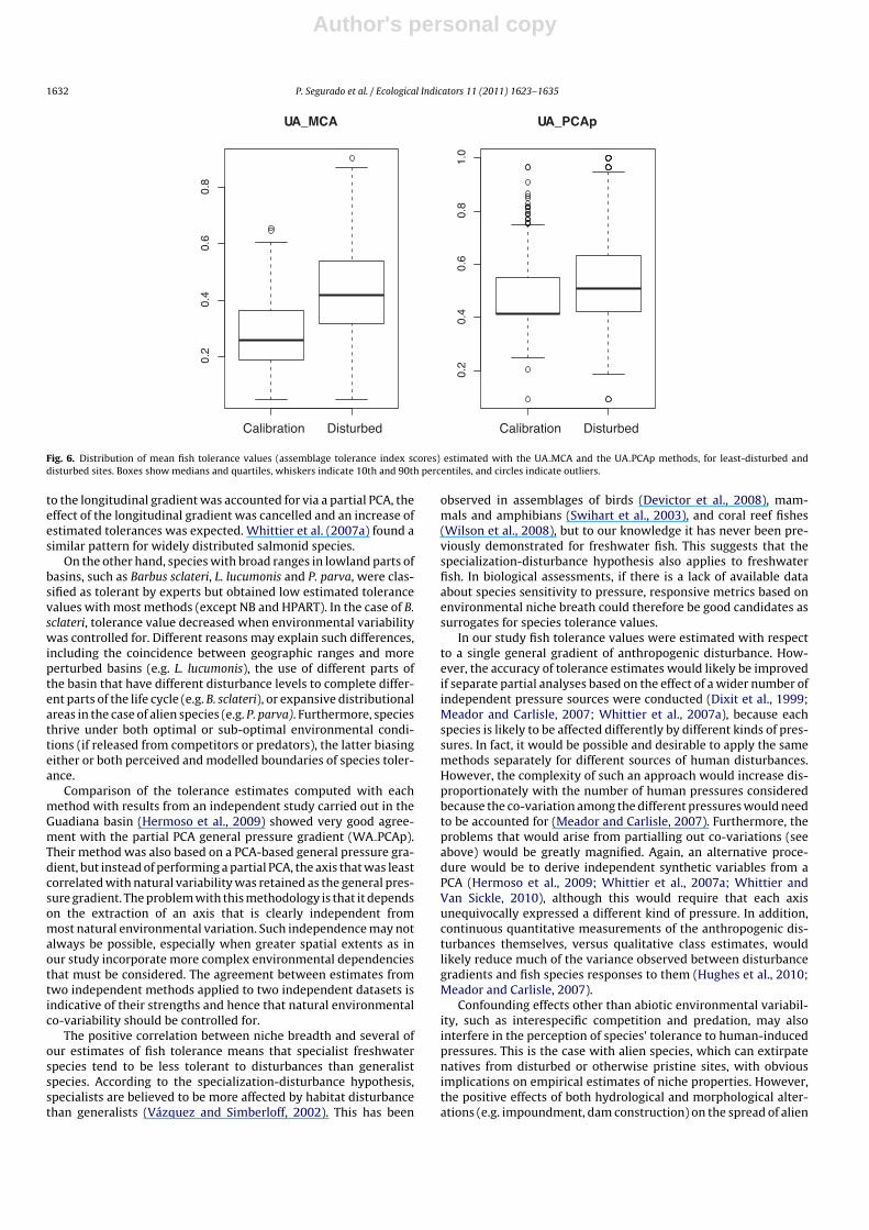
When tolerance values of all species were averaged to pro-duce an assemblage tolerance index for each site, least-disturbed(calibration) sites showed lower assemblage tolerance index val-ues than disturbed sites (Mann–Whitney U test, P < 0.001; Fig. 6).However, this difference is less evident when natural variability isaccounted for by means of a partial PCA.

4. Discussion

The tolerance classification of individual fish species to humanperturbation is an important step in most studies related to thedevelopment of ecological indicators of ecosystem quality, such asassemblage tolerance indices (Whittier et al., 2007a; Whittier andVan Sickle, 2010) and multi-metric indices of biological condition(Roset et al., 2007; Whittier et al., 2007b). Usually, tolerance classifi-cation is based on integrating knowledge from ecological studies ofparticular species, field observations, national conservation classifi-cations or anecdotal information. When regional studies of speciesecology are inconclusive, or when minimally disturbed sites arenot available, we recommend using tolerance classifications basedon field data such as those used in our study to support expertjudgments.

We compared several quantitative methods to estimate fishspecies tolerances to human disturbances of Mediterraneanstreams. Even though we observed high uncertainty in the esti-mated tolerance values related to the choice of statistical method,some methods were more consistent than others. Furthermore, thetwo most consistent methods (UA MCA and WA MCA) were alsothose that best discriminated tolerance classes based on expertjudgment. These two methods were primarily based on the posi-tion of species along a general disturbance gradient, as measuredby the mean or other location statistics. The UA MCA incorporatedboth location and the relation between the used and available dis-

Author's personal copy

P. Segurado et al. / Ecological Indicators 11 (2011) 1623–1635 1631

0 0.1 0.2 0.3 0.4 0.5 0.6 0.7 0.8 0.9

Liza ramadaMugil cephalus

Micropterus salmoidesLepomis gibbosusCarassius auratus

Gambusia holbrookiPlatichthys flesus

Cyprinus carpioParachondrostoma miegii

Barbus bocageiAtherina boyeriBarbus graellsii

Chelon labrosusCobitis paludicaBarbus barbus

Gobio gobioPetromyzon marinus

Gobio lozanoiPseudochondrostoma polylepis

Ameiurus melasRutilus rutilus

Anguilla anguillaBarbatula quignardi

Salaria fluviatilisPhoxinus bigerri

Squalius alburnoidesAustraloheros facetusOncorhynchus mykiss

Squalius pyrenaicusBarbus microcephalus

Leuciscus cephalusLampetra fluviatilisAlburnus alburnus

Iberochondrostoma lusitanicumPseudochondrostoma duriense

Squalius carolitertiiAchondrostoma oligolepis

Leuciscus souffiaGasterosteus gymnurus

Barbus tyberinusPseudochondrostoma willkommii

Rutilus rubilioPadogobius nigricansPadogobius martensii

Cobitis calderoniBarbus sclateriBarbus comizo

Lampetra planeriSalmo salar

Salmo trutta farioBarbus haasi

Leuciscus lucumonisCobitis taenia

Pseudorasbora parvaChondrostoma genei

Iberochondrostoma almacaiSqualius aradensis

Iberochondrostoma lemmingiiAchondrostoma arcasii

Anaecypris hispanica

General pressure gradient

Fig. 5. Used (grey bars) versus available (black lines) gradient of pressures based onMCA within each species’ potential range. Species are ranked in decreasing order oftolerance values estimated with the UA MCA method.

turbance gradient for each species, and slightly outperformed themethod based only on weighted averaging. The same core meth-ods were used by Dixit et al. (1999), Whittier et al. (2007a), andWhittier and Van Sickle (2010) in their tolerance evaluations.

Methods based on deviations from expected species occur-rences were limited to a few species with a sufficient number ofleast-disturbed sites for calibrating valid statistical models. For thisreason their comparison with the other methods is limited becausethey were based on fewer species. In addition, those methods arenot applicable to most alien species, which are usually absent fromleast-disturbed sites. Nevertheless, they were able to discriminatebetween species classified as intolerant and species classified asintermediate and tolerant.

The use of hierarchical partitioning to quantify the independenteffect of pressure on species distribution yielded the least consis-tent results. The problem with this approach is that the percentageof the independent contribution of the pressure gradient is relativeto the total explained variation. Most likely the models will greatlydiffer among species in their abilities to explain variation in data.Consequently, the independent percentage contribution could belarge for a given species, although representing just a small fractionof the total variation in the data.

Attempts to account for the effect of natural environmental co-variability generally produced tolerance estimates having weakerrelationships with tolerance classifications based on expert judg-ment. There are two possible explanations for this result. Thenatural environmental and pressure gradients may share a largeproportion of the explained variation in species occurrence (Steelet al., 2010). Therefore, when the shared variation is cancelled, onlya small proportion of variation of species occurrence explained bythe pressure gradient remains, which necessarily does not reflectits actual relative contribution. In other words, even if there is astrong effect of the pressure gradient, it may be masked by the nat-ural environmental variability, such that it is very difficult to testwhich gradient is truly affecting fish.

An alternative explanation for the lack of agreement is thatexpert judgments are also biased by not accounting for naturalvariability. This problem is likely exacerbated in Mediterraneanregions, where many fish species have very restricted distributionsand natural conditions create harsh aquatic environments withstrong/frequent winter floods, and summer droughts, resulting insubstantial physical and chemical stress. For example, I. almacai,which was classified as an intolerant species by experts, is restrictedto a few small basins in southernmost Portugal that are generallyless disturbed. Although this may cause experts to view the speciesas intolerant, the absence of this species from more disturbed basinsmay result more from historical factors than from species sensitiv-ity to pressure. Indeed, for this species, higher tolerance estimateswere found when methods that accounted for natural environ-mental variability were used. Also, experts may tend to classify as‘intermediate’ the less studied species which typically occur lessfrequently. Indeed, species classified as ‘intermediate’ occurred at106 sites, while those classified as ‘tolerant’ occurred at 301 sites(Tables 1 and 2).

An increase of estimated tolerance value was the general trendfor species classified as intolerant when a general disturbance gra-dient accounting for natural environmental variability was used.This is particularly true for species such as Salmo trutta fario andA. arcasii. Both species have a large potential geographical range,although they are restricted to headwaters or middle-sized streams(Doadrio, 2001), which are typically less influenced by human-induced disturbances. As a consequence, when the whole naturallongitudinal gradient is considered in tolerance quantification, anunderestimation of species tolerance value is inevitable becausethe natural longitudinal gradient is also a disturbance gradient.When only the component of disturbance variation not attributed

Author's personal copy

1632 P. Segurado et al. / Ecological Indicators 11 (2011) 1623–1635

Calibration Disturbed

0.2

0.4

0.6

0.8

UA_MCA

Calibration Disturbed

0.2

0.4

0.6

0.8

1.0

UA_PCAp

Fig. 6. Distribution of mean fish tolerance values (assemblage tolerance index scores) estimated with the UA MCA and the UA PCAp methods, for least-disturbed anddisturbed sites. Boxes show medians and quartiles, whiskers indicate 10th and 90th percentiles, and circles indicate outliers.

to the longitudinal gradient was accounted for via a partial PCA, theeffect of the longitudinal gradient was cancelled and an increase ofestimated tolerances was expected. Whittier et al. (2007a) found asimilar pattern for widely distributed salmonid species.

On the other hand, species with broad ranges in lowland parts ofbasins, such as Barbus sclateri, L. lucumonis and P. parva, were clas-sified as tolerant by experts but obtained low estimated tolerancevalues with most methods (except NB and HPART). In the case of B.sclateri, tolerance value decreased when environmental variabilitywas controlled for. Different reasons may explain such differences,including the coincidence between geographic ranges and moreperturbed basins (e.g. L. lucumonis), the use of different parts ofthe basin that have different disturbance levels to complete differ-ent parts of the life cycle (e.g. B. sclateri), or expansive distributionalareas in the case of alien species (e.g. P. parva). Furthermore, speciesthrive under both optimal or sub-optimal environmental condi-tions (if released from competitors or predators), the latter biasingeither or both perceived and modelled boundaries of species toler-ance.

Comparison of the tolerance estimates computed with eachmethod with results from an independent study carried out in theGuadiana basin (Hermoso et al., 2009) showed very good agree-ment with the partial PCA general pressure gradient (WA PCAp).Their method was also based on a PCA-based general pressure gra-dient, but instead of performing a partial PCA, the axis that was leastcorrelated with natural variability was retained as the general pres-sure gradient. The problem with this methodology is that it dependson the extraction of an axis that is clearly independent frommost natural environmental variation. Such independence may notalways be possible, especially when greater spatial extents as inour study incorporate more complex environmental dependenciesthat must be considered. The agreement between estimates fromtwo independent methods applied to two independent datasets isindicative of their strengths and hence that natural environmentalco-variability should be controlled for.

The positive correlation between niche breadth and several ofour estimates of fish tolerance means that specialist freshwaterspecies tend to be less tolerant to disturbances than generalistspecies. According to the specialization-disturbance hypothesis,specialists are believed to be more affected by habitat disturbancethan generalists (Vázquez and Simberloff, 2002). This has been

observed in assemblages of birds (Devictor et al., 2008), mam-mals and amphibians (Swihart et al., 2003), and coral reef fishes(Wilson et al., 2008), but to our knowledge it has never been pre-viously demonstrated for freshwater fish. This suggests that thespecialization-disturbance hypothesis also applies to freshwaterfish. In biological assessments, if there is a lack of available dataabout species sensitivity to pressure, responsive metrics based onenvironmental niche breath could therefore be good candidates assurrogates for species tolerance values.

In our study fish tolerance values were estimated with respectto a single general gradient of anthropogenic disturbance. How-ever, the accuracy of tolerance estimates would likely be improvedif separate partial analyses based on the effect of a wider number ofindependent pressure sources were conducted (Dixit et al., 1999;Meador and Carlisle, 2007; Whittier et al., 2007a), because eachspecies is likely to be affected differently by different kinds of pres-sures. In fact, it would be possible and desirable to apply the samemethods separately for different sources of human disturbances.However, the complexity of such an approach would increase dis-proportionately with the number of human pressures consideredbecause the co-variation among the different pressures would needto be accounted for (Meador and Carlisle, 2007). Furthermore, theproblems that would arise from partialling out co-variations (seeabove) would be greatly magnified. Again, an alternative proce-dure would be to derive independent synthetic variables from aPCA (Hermoso et al., 2009; Whittier et al., 2007a; Whittier andVan Sickle, 2010), although this would require that each axisunequivocally expressed a different kind of pressure. In addition,continuous quantitative measurements of the anthropogenic dis-turbances themselves, versus qualitative class estimates, wouldlikely reduce much of the variance observed between disturbancegradients and fish species responses to them (Hughes et al., 2010;Meador and Carlisle, 2007).

Confounding effects other than abiotic environmental variabil-ity, such as interespecific competition and predation, may alsointerfere in the perception of species’ tolerance to human-inducedpressures. This is the case with alien species, which can extirpatenatives from disturbed or otherwise pristine sites, with obviousimplications on empirical estimates of niche properties. However,the positive effects of both hydrological and morphological alter-ations (e.g. impoundment, dam construction) on the spread of alien

Author's personal copy

P. Segurado et al. / Ecological Indicators 11 (2011) 1623–1635 1633

species are well documented (Moyle and Light, 1996; Hughes et al.,2005). As a consequence, the effect of alien species on native specieswas indirectly incorporated into the empirical tolerance estimates.

5. Conclusions

In conclusion, expert judgment classifications of tolerance com-monly used in bioassessment can be biased by personal fieldexperience and anecdotal information. Therefore, we recommendthat scientists confront, correct and supplement these classifica-tions via empirical data modelling (Dixit et al., 1999; Whittier et al.,2007a; Whittier and Van Sickle, 2010). The same need applies tocontinents where quantitative environmental databases are justbeginning to be developed and species tolerances are less known(e.g. Cassati et al., 2006; Moya et al., 2011).

The present work represents the most comprehensive attemptto date to evaluate alternative methods of quantifying fishtolerances to human-induced pressures. This was particularlydemanding given the geographical extent of the study area(Northwest Mediterranean region), the difficulties imposed by theenvironmental extremes of naturally flashy Mediterranean rivers,the high level of endemic species with restricted geographicalranges (Moyle and Marchetti, 1999), and incomplete ecologicalknowledge concerning many species (Ferreira et al., 2007). Further-more, Mediterranean landscapes have been extensively shaped byhuman activities for centuries, affecting the fluvial ecosystems inmany different and interacting ways (Pont et al., 2009b), whichhinders properly identifying undisturbed sites.

Overall, methods based on the concepts of niche breath andniche position yielded the most consistent results with previousexpert-based tolerance ranges, namely those based on weightedaveraging and on the “used versus available” pressure gradients.Our results suggest that there is a strong joint contribution ofnatural environmental variability with the general degradation gra-dient, making it very difficult to assess unequivocally the effectthat most determines species distributions. However, methods thatdid not account for natural environmental variability yielded tol-erance values that were more in agreement with expert judgment,although, as mentioned above, this agreement may be misleading.More robust tolerance estimates should therefore rely on samplingdesigns specifically oriented to explicitly disentangling the effectsof human-induced pressures and natural variability.

Nonetheless, we recommend the use of two alternative meth-ods, depending on the species and the extent of the gradient understudy. If the study area encompasses a wide range of the abioticvariability within the target species’ geographical range, we rec-ommend the use of average weighting based on the gradient froma partial PCA (WA PCAp). This method is simple to implement andshowed the strongest agreement with results of an independentstudy. If the targeted area is more restricted and contains only asmall portion of the abiotic variability within the species’ geograph-ical range, we recommend the use of the “used versus available”approach based on a MCA (UA MCA). This method has the advan-tage of computing tolerance values that are relative to the availablepressure gradient which, in this case, would be necessarily nar-rower.

Acknowledgements

This study was funded by the European Commission underthe Sixth Framework Programme (EFI+ project, contract number044096). P. Segurado was supported by a grant from Fundacão paraa Ciência e Tecnologia (SFRH/BPD/39067/2007) and R.M. Hughesby a Fulbright Brasil grant. Many people contributed with theirexpertise to the tolerance classification used in this work: P. Bady,

K. Battes, M. Beers, J. Belliard, P. Bohman, T. Buijse, I.G. Cowx,J. Gortázar, G. Haidvogl, B. Halasi-Kovács, S. Holzer, M. Logez, G.Maio, R.A.A. Noble, P. Pinheiro, P. Prus, E. Schager, R. Schinegger, S.Schmutz, N. Schotzko, T. Sutela, C. Trautwein, T. Vehanen, W. Wis-niewolski, and C. Wolter. We also thank the many field biologists,too numerous to mention, that provided the fish and environmentaldata.

Appendix A. Factor loadings of the Smith–Hill ordinationusing environmental variables based on geomorphologiccharacteristics

Variable Categories Axis 1 Axis 2

Geomorphologicalriver type

Braided −0.39 −0.30Constraint 0.36 −0.12Meand −0.71 0.97Sinuous 0.09 −0.22

Distance from source −0.50 −0.46Size of catchment −0.44 −0.56

Former floodplain No 0.25 −0.22Yes −0.89 0.79

Valley shape Gorges 0.41 −0.44Plains −0.98 0.66U shape 0.10 0.24V shape 0.22 −0.17

Appendix B. Types of pressures and single variablesconsidered (from EU-project EFI+ http://efi-plus.boku.ac.at)

Pressure type Single pressurevariables

Score

Connectivity Presence of barriersupstream of the riversegment

No (1), partial (3), yes(4)

Presence of barriersdownstream of theriver segment

No (1), partial (3), yes(4)

Hydrology Impoundment No (1), weak (3), strong(5)

Hydropeaking No (1), partial (3), yes(4)

Water abstraction No (1), weak (3), strong(5)

Hydrologicalmodifications

No (1), yes (3)

Morphology Channelization No (1), intermediate(3), straightened (5)

U-shaped cross section No (1), intermediate(3), yes (5)

Instream habitatalterations

No (1), slight (2), high(5)

Riparian vegetationalteration

No (1), local (2),intermediate (3), high(5)

Leveed No (1), continuouspermeable (3),continuousimpermeable (5)

Water quality Toxic substances No (1), Intermediate(3), high (5)

Acidification No (1), yes (3)Eutrophication No (1), low (3),

intermediate (4),extreme (5)

Organic pollution No (1), weak (3), strong(5)

Organic siltation No (1), yes (3)Water Quality IndexScore

1 (good quality)–5(poor quality)

Author's personal copy

1634 P. Segurado et al. / Ecological Indicators 11 (2011) 1623–1635

Appendix C. List of the expert leaders involved in the fishtolerance classification

Name Institution Country

Battes, Klaus The Bacau University, Facultyof Sciences

Romania

Buijse, Tom DELTARES, Department ofFreshwater Ecology & WaterQuality, Utrecht

Netherlands

Ferreira, Teresa Instituto Superior deAgronomia, Lisbon

Portugal

Garcia de Jalon, Diego Universidad Politécnica deMadrid

Spain

Maio, Guiseppe AQUAPROGRAM s.r.l., Vicenza ItalyMelcher, Andreas BOKU, University of natural

resources and life sciences,Vienna

Austria

Noble, Richard Hull International FisheriesInstitute (HIFI), University ofHull

United Kingdom

Pont, Didier Cemagref, Aix en Provence FranceSchager, Eva EAWAG, Swiss Federal

Institute of Aquatic Science andTechnology, Kastanienbaum

Switzerland

Schotzko, Nikolaus BAW, Federal Agency for WaterManagement, Institute forWater Ecology, Fisheries andLake Research,Scharfling/Mondsee

Austria

Vehanen, Teppo Finnish Game and FisheriesResearch Institute, Uleåborg

Finland

Wisniewolski, Wieslaw Inland Fisheries Institute,Olsztyn

Poland

Wolter, Christian Institute of Freshwater Ecologyand Inland Fisheries, Berlin

Germany

References

Barbour, M.T., Gerritsen, J., Snyder, B.D., Stribling, J.B., 1999. Rapid BioassessmentProtocols for use in Streams and Wadeable Rivers: Periphyton, Benthic Macroin-vertebrates, and Fish. EPA 841/B-99/002, U.S. Environmental Protection Agency,Washington, D.C. www.epa.gov/owow/monitoring/rbp/wp61pdf/rbp main.pdf(accessed October 2010).

Bryce, S.A., Hughes, R.M., Kaufmann, P.R., 2002. Development of a bird integrityindex: using bird assemblages as indicators of riparian condition. Environ. Man-age. 30, 294–310.

Cassati, L., Langeani, F., Ferreira, C.P., 2006. Effects of physical habitat degradationon the stream fish assemblage structure in a pasture region. Environ. Manage.38, 974–982.

CEN (Comité Européen de Normalisation), 2003. Water Quality – Sampling of Fishwith Electricity. CEN, European Standard – EN 14011:2003 E, Brussels, Belgium.

Chevan, A., Sutherland, M., 1991. Hierarchical partitioning. Am. Stat. 45, 90–96.Chutter, F.M., 1972. An empirical biotic index of the quality of water in South African

streams and rivers. Water Res. 6, 19–30.Davies, S.P., Jackson, S.K., 2006. The biological condition gradient: a descrip-

tive model for interpreting change in aquatic ecosystems. Ecol. Appl. 16,1251–1266.

Devictor, V., Julliard, R., Jiguet, F., 2008. Distribution of specialist and generalistspecies along spatial gradients of habitat disturbance and fragmentation. Oikos117, 507–514.

Dixit, S.S., Smol, J.P., Charles, D.F., Hughes, R.M., Paulsen, S.G., Collins, G.B., 1999.Assessing water quality changes in the lakes of the northeastern United Statesusing sediment diatoms. Can. J. Fish. Aquat. Sci. 56, 131–152.

Doadrio, I., 2001. Atlas y Libro Rojo de los Peces Continentales de Espana. MuseoNacional de Ciencias Naturales, Madrid.

Ferreira, M.T., Oliveira, J., Caiola, N., de Sostoa, A., Casals, F., Cortes, R., Economou, A.,Zogaris, S., Garcia-Jalon, D., Ilhéu, M., Pont, D., Rogers, C., Prenda, J., 2007. Ecolog-ical traits of fish assemblages from Mediterranean Europe and their responsesto human disturbance. Fisheries Management and Ecology 14, 473–481.

Gasith, A., Resh, V.H., 1999. Streams in Mediterranean climate regions: abiotic influ-ences and biotic responses to predictable seasonal events. Annu. Rev. Ecol. Syst.30, 51–81.

Harrell Jr., F.E., 2001. Regression modeling strategies: with applications to linearmodels, logistic regression, and survival analysis. Springer-Verlag, New York.

Hastie, T.J., Tibshirani, R.J., 1990. Generalized Additive Models. Chapman and Hall,New York.

Hermoso, V., Clavero, M., Blanco-Garrido, F., Prenda, J., 2009. Assessing freshwaterfish sensitivity to different sources of perturbation in a Mediterranean basin.Ecol. Freshw. Fish 18, 269–281.

Hill, M.O., Smith, A.J.E., 1976. Principal component analysis of taxonomic data withmulti-state discrete characters. Taxon 25, 249–255.

Hilsenhoff, W.L., 1977. Use of arthropods to evaluate water quality of streams. Tech-nical Bulletin No. 100. Department of Natural Resources. Madison, Wisconsin,USA.

Hughes, R.M., Noss, R.F., 1992. Biological diversity and biological integrity: currentconcerns for lakes and streams. Fisheries 17 (3), 11–19.

Hughes, R.M., Herlihy, A.T., Kaufmann, P.R., 2010. An evaluation of qualitativeindexes of physical habitat applied to agricultural streams in ten U.S. states.J. Am. Water Resour. Assoc. 46, 792–806.

Hughes, R.M., Rinne, J.N., Calamusso, B., 2005. Historical changes in large-river fishassemblages of the Americas: a synthesis. Am. Fish. Soc. Symp. 45, 603–612.

Jongman, R.H.G., ter Braak, C.J.F., Van Tongeren, O.F.R., 1995. Data Analysis in Com-munity and Landscape Ecology. Cambridge University Press, Cambridge.

Kolkwitz, R., Marsson, K., 1909. Ökologie der tierischen saprobien: beiträge zur lehrevon des biologischen gewasserbeurteilung. Internationale Revue der GesamtenHydrobiologie und Hydrographie 2, 126–152.

McCullagh, P., Nelder, J.A., 1989. Generalized Linear Models, second ed. Chapmanand Hall, New York, NY.

Meador, M.R., Carlisle, D.M., 2007. Quantifying tolerance indicator values for com-mon stream fish species of the United States. Ecol. Indic. 7, 329–338.

Melcher, A., Schmutz, S., Haidvogl, G., Moder, K., 2007. Spatially based methods toassess the ecological status of European fish assemblage types. Fish. Manag. Ecol.14, 453–463.

Moya, N., Hughes, R.M., Dominguez, E., Gibon, F.-M., Goita, E., Oberdorff, T., 2011.Macroinvertebrate-based multimetric predictive models for evaluating thehuman impact on biotic condition of Bolivian streams. Ecol. Indic. 11, 840–847.

Moyle, P.B., Light, T., 1996. Biological invasions of freshwater: empirical rules andassembly theory. Biol. Conserv. 78, 149–161.

Moyle, P.B., Marchetti, M.P., 1999. Applications of indices of biotic integrity to Cali-fornia streams and watersheds. In: Simon, T.P. (Ed.), Assessing the Sustainabilityand Biological Integrity of Water Resources Using Fish Communities. CRC Press,Boca Raton, FL, pp. 367–380.

Oberdorff, T., Pont, D., Hugueny, B., Porcher, J.P., 2002. Development and validationof a fish-based index (FBI) for the assessment of French rivers: a framework forenvironmental assessment. Freshw. Biol. 46, 399–415.

Paulsen, S.G., Mayio, A., Peck, D.V., Stoddard, J.L., Tarquinio, E., Holdsworth, S.M.,Van Sickle, J., Yuan, L.L., Hawkins, C.P., Herlihy, A., Kaufmann, P.R., Barbour, M.T.,Larsen, D.P., Olsen, A.R., 2008. Condition of stream ecosystems in the US: anoverview of the first national assessment. J. N. Am. Benthol. Soc. 27, 812–821.

Pirhalla, D.E., 2004. Evaluating fish-habitat relationships for refining regionalindexes of biotic integrity: development of a tolerance index of habitat degra-dation for Maryland stream fishes. Trans. Am. Fish. Soc. 133, 144–159.

Plafkin, J.L., Barbour, M.T., Porter, K.D., Gross, S.K., Hughes, R.M., 1989. RapidBioassessment Protocols for use in Streams and Rivers: Benthic Macroinver-tebrates and Fish. EPA/444/4-89/001. U.S. Environmental Protection Agency,Washington, DC.

Pont, D., Hughes, R.M., Whittier, T.R., Schmutz, S., 2009a. A predictive index of bioticintegrity model for aquatic-vertebrate assemblages of western U.S. streams.Trans. Am. Fish. Soc. 138, 292–305.

Pont, D., Hugueny, B., Beier, U., Goffaux, D., Melcher, A., Noble, R., Rogers, C., Roset,N., Schmutz, S., 2006. Assessing river biotic condition at the continental scale: aEuropean approach using functional metrics and fish assemblages. J. Appl. Ecol.43, 70–80.

Pont, D., Hugueny, B., Rogers, C., 2007. Development of a fish-based index for theassessment of river health in Europe: the European Fish Index. Fish. Manag. Ecol.14, 427–439.

Pont, D., Piegay, H., Farinetti, A., Allain, S., Landon, N., Liebault, F., Dumont,B., Richard-Mazet, A., 2009b. Conceptual framework and interdisciplinaryapproach for the sustainable management of gravel-bed rivers: the case of theDrome River basin (S.E. France). Aquat. Ecol. 71, 356–370.

R Development Core Team, 2007. R: a language and environment for statistical com-puting. R Foundation for Statistical Computing. Vienna, Austria. Geobotanica 13,49–67.

Reyjol, Y., Hugueny, B., Pont, D., Bianco, P.G., Beier, U., Caiola, N., Casals, F., Cowx,I., Economou, A., Ferreira, T., Haidvogl, G., Noble, R., Sostoa, A., Vigneron, T.,Virbickas, T., 2007. Patterns in species richness and endemism of Europeanfreshwater fish. Global Ecol. Biogeogr. 16, 65–75.

Rivas-Martínez, S., Loidi-Arregui, J., 1999. Bioclimatoloy of the Iberian Peninsula.Itinera Geobotanica 13, 41–47.

Roset, N., Grenouillet, G., Goffaux, D., Pont, D., Kestemont, P., 2007. A review ofexisting fish assemblage indicators and methodologies. Fish. Manag. Ecol. 14,393–405.

Rowe, G., Wright, G., 1999. The Delphi technique as a forecasting tool: issues andanalysis. Int. J. Forecast. 15 (4), 353–375.

Schmutz, S., Melcher, A., Frangez, C., Haidvogl, G., Beier, U., Böhmer, J., Breine, J.,Simoens, I., Caiola, N., de Sostoa, A., Ferreira, M.T., Oliveira, J., Grenouillet, G.,Goffaux, D., deLeuuw, J.J., Noble, R.A.A., Roset, N., Verbickas, T., 2007. Spatiallybased methods to assess the ecological status of riverine fish assemblages inEuropean ecoregions. Fish. Manag. Ecol. 14, 441–452.

Steel, A., Hughes, R.M., Schmutz, S., Muhar, S., Poppe, M., Trautwein, C., Fukushima,M., Shimazaki, H., Young, J., Feist, B., Fullerton, A., Sanderson, B., 2010. Meet-ing the challenges of landscape scale riverine research: a review. Living Rev.Landscape Res. 4, 1–60.

Stolte, K.W., Mangis, D.R., 1992. Identification and use of plant species as ecologi-cal indicators of air pollution stress in national park units. In: McKenzie, D.H.,

Author's personal copy

P. Segurado et al. / Ecological Indicators 11 (2011) 1623–1635 1635

Hyatt, D.E., McDonald, V.J. (Eds.), Ecological Indicators. Elsevier, New York, pp.373–392.

Swihart, R.K., Gehrig, T.M., Kolozsvary, M.B., Nupp, T.E., 2003. Responses of ‘resistant’vertebrates to habitat loss and fragmentation: the importance of niche breadthand range boundaries. Divers. Distrib. 9, 1–18.

ter Braak, C.J.F., 1995. Ordination. In: Jongman, C.J., ter Braak, F., Tongeren, V. (Eds.),Data Analysis in Community and Landscape Analysis. Cambridge UniversityPress, Cambridge, pp. 91–173.

Thioulouse, J., Chessel, D., Doledec, S., Olivier, J.M., 1997. ADE-4: a multivariateanalysis and graphical display software. Stat. Comput. 7, 75–83.

Vázquez, D.P., Simberloff, D., 2002. Ecological specialization and susceptibility todisturbance: conjectures and refutations. Am. Nat. 159, 606–623.

Venables, W.N., Ripley, B.D., 1997. Modern Applied Statistics with S-PLUS. Springer,New York.

Vogt, J., Soille, P., de Jager, A., Rimaviciute, E., Mehl, W., Foisneau, S., Bodis, K., Dusart,J., Paracchini, M.L., Haastrup, P., Bamps, C., 2007. A pan-European River andCatchment Database. European Commission – JRC, Luxembourg (EUR 22920 EN).

Whittier, T.R., Hughes, R.M., 1998. Evaluation of fish species tolerances to envi-ronmental stressors in lakes of the northeastern United States. N. Am. J. Fish.Manage. 18, 236–252.

Whittier, T.R., Van Sickle, J., 2010. Macroinvertebrate tolerance values and an assem-blage tolerance index (ATI) for western USA streams and rivers. J. N. Am. Benthol.Soc. 29, 852–866.

Whittier, T.R., Hughes, R.M., Lomnicky, G.A., Peck, D.V., 2007a. Fish and amphibiantolerance values and an assemblage tolerance index for streams and rivers inthe western USA. Trans. Am. Fish. Soc. 136, 254–271.

Whittier, T.R., Hughes, R.M., Stoddard, J.L., Lomnicky, G.A., Peck, D.V., Herlihy, A.T.,2007b. A structured approach to developing indices of biotic integrity: threeexamples from western USA streams and rivers. Trans. Am. Fish. Soc. 136,718–735.

Wilson, S.K., Burgess, S.C., Cheal, A.J., Emslie, M., Fisher, R., Miller, I., Polunin,N.V., Sweatman, H.P., 2008. Habitat utilization by coral reef fish: implicationsfor specialists vs. generalists in a changing environment. J. Anim. Ecol. 77,220–228.

Yuan, L.L., 2004. Assigned macroinvertebrate tolerance classifications using gener-alized additive models. Freshw. Biol. 49, 662–677.

Yuan, L.L., 2006. Estimation and Application of Macroinvertebrate Tolerance Values.EPA/600/P-04/116F. U.S. Environmental Protection Agency, Washington, DC.