Estimating soil moisture using remote sensing data: A machine learning approach

Advances in Water Resources 33 (2010) 69–80

Contents lists available at ScienceDirect

Advances in Water Resources

journal homepage: www.elsevier .com/ locate/advwatres

Estimating soil moisture using remote sensing data: A machine learning approach

Sajjad Ahmad *, Ajay Kalra, Haroon StephenDepartment of Civil and Environmental Engineering, University of Nevada, 4505 Maryland Parkway, Las Vegas, NV 89154-4015, United States

a r t i c l e i n f o

Article history:Received 8 June 2009Received in revised form 27 September2009Accepted 20 October 2009Available online 25 October 2009

Keywords:SVMANNSoil moistureBackscatterNDVIRemote sensingTRMM

0309-1708/$ - see front matter � 2009 Elsevier Ltd. Adoi:10.1016/j.advwatres.2009.10.008

* Corresponding author. Tel.: +1 702 895 5456; faxE-mail address: [email protected] (S. Ahmad

a b s t r a c t

Soil moisture is an integral quantity in hydrology that represents the average conditions in a finite vol-ume of soil. In this paper, a novel regression technique called Support Vector Machine (SVM) is presentedand applied to soil moisture estimation using remote sensing data. SVM is based on statistical learningtheory that uses a hypothesis space of linear functions based on Kernel approach. SVM has been usedto predict a quantity forward in time based on training from past data. The strength of SVM lies in min-imizing the empirical classification error and maximizing the geometric margin by solving inverse prob-lem. SVM model is applied to 10 sites for soil moisture estimation in the Lower Colorado River Basin(LCRB) in the western United States. The sites comprise low to dense vegetation. Remote sensing datathat includes backscatter and incidence angle from Tropical Rainfall Measuring Mission (TRMM), andNormalized Difference Vegetation Index (NDVI) from Advanced Very High Resolution Radiometer(AVHRR) are used to estimate soil water content (SM). Simulated SM (%) time series for the study sitesare available from the Variable Infiltration Capacity Three Layer (VIC) model for top 10 cm layer of soilfor the years 1998–2005. SVM model is trained on 5 years of data, i.e. 1998–2002 and tested on 3 yearsof data, i.e. 2003–2005. Two models are developed to evaluate the strength of SVM modeling in estimat-ing soil moisture. In model I, training and testing are done on six sites, this results in six separate SVMmodels – one for each site. Model II comprises of two subparts: (a) data from all six sites used in modelI is combined and a single SVM model is developed and tested on same sites and (b) a single model isdeveloped using data from six sites (same as model II-A) but this model is tested on four separate sitesnot used to train the model. Model I shows satisfactory results, and the SM estimates are in good agree-ment with the estimates from VIC model. The SM estimate correlation coefficients range from 0.34 to 0.77with RMSE less than 2% at all the selected sites. A probabilistic absolute error between the VIC SM andmodeled SM is computed for all models. For model I, the results indicate that 80% of the SM estimateshave an absolute error of less than 5%, whereas for model II-A and II-B, 80% and 60% of the SM estimateshave an error less than 10% and 15%, respectively. SVM model is also trained and tested for measured soilmoisture in the LCRB. Results with RMSE, MAE and R of 2.01, 1.97, and 0.57, respectively show that theSVM model is able to capture the variability in measured soil moisture. Results from the SVM modelingare compared with the estimates obtained from feed forward-back propagation Artificial Neural Networkmodel (ANN) and Multivariate Linear Regression model (MLR); and show that SVM model performs bet-ter for soil moisture estimation than ANN and MLR models.

� 2009 Elsevier Ltd. All rights reserved.

1. Introduction

Soil moisture is an important variable for understandinghydrology and climate. Its distribution is of great importance inthe hydrological cycle due to its high spatial and temporal variabil-ity. Soil moisture has a strong influence on the relative distributionof water between various components of the hydrological cycle[54,17,20]. Accurate measurements of the antecedent soil moistureconditions are important for accurate event based hydrologicalsimulations in different soil wetness states [18].

ll rights reserved.

: +1 702 895 3936.).

The ongoing drought of the Colorado River Basin in the SouthWestern United States started in 2000 and has become the longestdrought in the recorded history of the basin. Due to the regionalimportance of this basin, it is important to understand the factorsrelated to this drought [54,39,10]. Drought signatures are closelyrelated to the spatial and temporal variability of soil moisture.Accurate soil moisture information can provide insight intodrought condition.

Radar backscatter ðr�Þ with its sensitivity to dielectric proper-ties is useful in mapping land surface soil moisture [37,7,36,6]. Re-cent research directions indicate rising interest in the operationalmeasuring and monitoring of the global soil moisture using remotesensing [35,33,52]. National Aeronautics and Space Administration

70 S. Ahmad et al. / Advances in Water Resources 33 (2010) 69–80

plans to launch a dedicated soil moisture mapping mission calledSoil Moisture Active Passive (SMAP) in 2012 [5]. Similar missioncalled Soil Moisture and Ocean Salinity (SMOS) is to be launchedby European Space Agency in 2009 [14]. Retrieving soil moisturefrom microwave remote sensing measurements is an active andchallenging area of research.

Various theoretical and empirical models have been devised toretrieve soil moisture from active and passive remote sensing data[48,15,40,53,12]. Theoretical models involve complicated scatter-ing phenomena from probabilistic models of soil, vegetation, andterrain whereas empirical models capture relationships amongmeasured variables to estimate geophysical characteristics. Theo-retical models are data driven but require in situ data for calibra-tion and validation. In situ data is not widely available and issparse for regional scale modeling. In addition to limited availabil-ity of measured soil moisture data, decoupling the effects of soiland vegetation on r� also poses a major difficulty for useful appli-cation [55]. The presence of vegetation reduces r� sensitivity tosoil moisture. In order to achieve accurate soil moisture estimatesand avoid above-mentioned difficulties, a need for data-drivenmodel is felt, which can efficiently relate the inputs to the desiredoutput and is not computationally intensive.

Artificial Neural Networks (ANN) are models that learn from atraining data set mimicking the human-learning ability. They arerobust to noisy data and can approximate multivariate non-linearrelations among the variables [47]. ANN’s have been used for awide range of different learning-from-data applications and in-put–output correlations of non-linear processes in water resources,and hydrology [30,1,21,57]. The structure and operation of ANN isdiscussed by a number of authors [1,21,57,9,44,22]. A review ofANN applications in hydrology is available in the ASCE task com-mittee report [3].

Recently, another data-driven model, i.e. Support Vector Ma-chine (SVM) has gained popularity in many ANN dominated fieldsand has attracted the attention of many researchers[28,23,29,4,56,24,45]. SVMs are considered as kernel based learn-ing systems rooted in the statistical learning theory and structuralrisk minimization [19]. SVMs have been successfully applied forpattern recognition and regression in different fields such as bio-informatics and artificial intelligence. There are also a few applica-tions of SVM in hydrology. Lin et al. [28] used SVM to forecasthourly typhoon rainfall in Fei-Tsui Reservoir Watershed in north-ern Taiwan and compared the results with ANN model. Kalra andAhmad [23] applied SVM for long lead streamflow forecastingusing oceanic oscillations in the Upper Colorado River Basin. Liongand Sivapragasam [29] indicated a superior SVM performance overANN in forecasting flood stages for the Bangladesh River system.Asefa et al. [4] applied SVM to forecast flows at seasonal and hourlytime scale for the Sevier River Basin. Dibike et al. [13] applied SVMfor rainfall/runoff modeling and classification of digital remotesensing image data and compared results with ANN. Gill et al.[16] applied SVM for predicting soil moisture for four and sevendays in advance using meteorological variables and comparedthe results with ANN model. SVMs soil moisture predictions werea good match with the actual soil moisture data and SVM modelperformed better than ANN model. It is noteworthy that in allthe above-mentioned applications, the SVM modeling results arebetter than results obtained from ANN models due to the high gen-eralization characteristic of SVM models.

In this research, we relate TRMMPR backscatter to volumetricsoil moisture content (%) and vegetation using SVM data-drivenmodel. SVM is presented for temporal estimation of Variable Infil-tration Capacity (VIC) soil moisture using remote sensing data atselected sites in the Lower Colorado River Basin. The selected siteshave varying vegetation cover comprising of low, medium, anddense vegetation. SVM model is also trained and tested using

ground soil moisture data for a site in Walnut Gulch ExperimentalWatershed (WGEG) in LCRB. Besides SVM, a feed forward-backpropagation ANN model and a multivariate linear regression(MLR) model are also developed to estimate temporal soil mois-ture. The soil moisture estimates using different models arecompared.

The paper is organized as follows: Section 2 presents theoreticalbackground of SVM. The study region and the data used are de-scribed in Sections 3 and 4, respectively. In Section 5, the proposedmethod to estimate soil moisture is presented. Section 6 describesthe results and discussion of soil moisture estimates obtainedusing SVM model (VIC SM estimates and ground measured soilmoisture) and comparison of SVM model results with that ofANN and MLR models. Section 7 summarizes and concludes thepaper.

2. Support vector machines

The idea of learning machines was first proposed by Turing. Thetrainer of learning machine is ignorant of the processes undergoinginside it, which is considered to be the most important feature ofthe machine [46]. The SVM was developed by Vapnik and co-work-ers in the early 1990s for the purpose of classification. Later, Vap-nik extended his work by developing SVMs for regression [49].There are two important factors to control the generalization abil-ity of the learning machine. The first factor is the error-rate on thetraining data, and the second factor is the capacity of the learningmachine measured in terms of Vapnik–Chervonenkis (VC) dimen-sions [51]. The non-linearities in the system being modeled werehandled by including kernels which act as building blocks for SVMsand are based on the requirements to satisfy Mercer’s theorem[49,50,11]. SVM are trained with a learning algorithm derived fromoptimization theory that uses a hypothesis space of linear func-tions in a higher dimensional feature space. The learning algorithmis then implemented in a learning bias derived from a statisticallearning theory [11].

When working with statistical learning tools, the ultimate goalis to find a functional dependency, f ðxÞ, between independent vari-ables fx1;x2; . . . :xLg obtained from x 2 RK . The (dependent) outputfy1; y2; . . . ; yLg is obtained from y 2 R selected from a set of L inde-pendent and identically distributed (i.i.d.) observations. The func-tional dependency is given by f ðxÞ ¼ hw;xi þ b where hw;xidenotes the dot product of a weighting vector w and input vectorx; and b is the bias. The observations are called the regularizedfunctionals, as shown in [50,42], and have the followingformulation:

Minimize12kwk2 þ C

XL

i¼1

ni þ n�i� �

Subject to

yi �PKj¼1

PLi¼1

wjxji � b 6 eþ ni;

PKj¼1

PLi¼1

wjxji þ b� yi 6 eþ n�i ;

ni; n�i P 0;

8>>>>>><>>>>>>:

ð1Þ

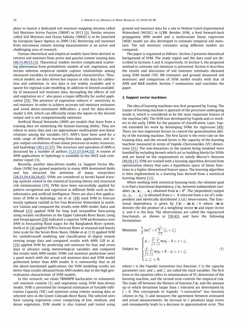
where e is the Vapniks insensitive loss function; C is the capacityparameter cost; and ni and n�i are called the slack variables. The firstterm in the equation refers to minimization of VC-dimension of thelearning machine, and the second term controls the empirical risk.The trade off between the flatness of function f ðxÞ and the amountup to which deviations larger than e tolerated are determined byC > 0. This corresponds to Vapniks ‘‘e-insensitive” loss function(shown in Fig. 1) and measures the agreement between estimatedand actual measurements. An increase in C penalizes large errorsand consequently leads to a decrease in approximation error. This

ξ

xx

x

x

xx

x

x

- ε

+ ε

x

y - f(x)

Loss

ξ

ε-εy

f(x)

Fig. 1. Pre-specified accuracy and slack variable n in SVM model.

S. Ahmad et al. / Advances in Water Resources 33 (2010) 69–80 71

is achieved by increasing the weight vector norm, kwk, which doesnot necessarily guarantee a good generalization performance of themodel. Slack variables, ni and n�i , determine the degree to whichsample points are penalized if the error is larger than e. Hence,for any (absolute) error smaller than e; ni ¼ n�i ¼ 0, and no datapoints are required for the objective function. This implies thatnot all the variables are used to estimate f ðxÞ. The functional depen-dency f ðxÞ is written as:

f ðxÞ ¼XK

j¼1

wjxj þ b; ð2Þ

where K is the number of support vectors.Another technique of solving the optimization problem, subject

to constraints in the loss function, is using the dual formulation. Indual formulation, Lagrange multipliers, a� and a, are introducedand the minimization equation is solved by differentiating with re-spect to the primary variables. It results in a maximization prob-lem, i.e.

Maximize

Wða�;aÞ ¼ �eXL

i¼1

ai þ a�i� �

þXL

i¼1

ðyi ai � a�i� �

Þ

� 12

XL

i;j¼1

ai � a�i� �

aj � a�j� �

kðxi; xjÞ

subject to the constraints

XL

i¼1

a�i � ai� �

¼ 0 and 0 6 ai; a�i 6 C; ð3Þ

where i = 1, . . . ,L is the sample size and the approximating functionis given by

f ðxÞ ¼XN

i¼1

a�i � ai� �

kðx; xiÞ þ b: ð4Þ

In Eqs. (3) and (4), a� and a are Lagrange multipliers; and kðx; xiÞ isthe kernel function that measures non-linear dependence betweenthe two input variables x, and xi. The xi’s are ‘‘support vectors”, andN (usually N � LÞ is the number of selected data points or supportvectors corresponding to values of the independent variable thatare at least e away from actual observations. The training patternin the dual formulation can be used to estimate the dot productof two vectors of any dimensions and is regarded as the advantageof the dual formulation [42]. This advantage in SVM is used to dealwith non-linear function approximations. Therefore, the steps in-volved in SVM modeling are: (1) selecting a suitable kernel functionand kernel parameter (kernel width – c); (2) specifying the ‘e’ insen-sitive parameter; and (3) specifying the capacity parameter cost,‘C’.Interested readers are referred to Kalra and Ahmad [23] for theillustration of working mechanism and example of SVM technique.

3. Study region

Colorado River basin provides water supply, flood control, andhydropower to a large area of the southwest United States. The ba-sin drains an area of 637,000 km2 (246,000 square miles), includingparts of seven western US states, Wyoming, Colorado, Utah, NewMexico, Nevada, Arizona, and California. It is one of the mostimportant river basins in the USA in terms of water supply for 25million people within the basin states and adjoining areas. Becauseof its geographic and climatologic characteristics, the Colorado Riv-er Basin is particularly vulnerable to severe and sustained drought.

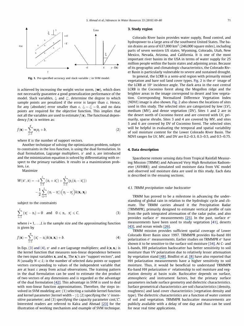
In general, the LCRB is a semi-arid region with primarily mixedvegetation and bare soil land cover types. Fig. 2 is the r� image ofthe LCRB at 10� incidence angle. The dark area in the east centralLCRB is the Coconino forest along the Mogollon ridge and thebrighter areas in the image correspond to desert and low vegeta-tion. Corresponding Normalized Difference Vegetation Index(NDVI) image is also shown. Fig. 2 also shows the locations of sitesused in this study. The selected sites are categorized by low (LV),medium (MV), and dense vegetation (DV). Sites 1 and 2 are inthe desert north of Coconino forest and are covered with LV, pri-marily, sparse shrubs. Sites 3 and 4 are covered by MV, and sites5 and 6 are covered by DV of Coconino forest. The selected siteswill be helpful in evaluating the temporal and spatial variabilityof soil moisture content for the Lower Colorado River Basin. TheNDVI ranges for LV, MV, and DV are 0.2–0.3, 0.3–0.5, and 0.5–0.75.

4. Data description

Spaceborne remote sensing data from Tropical Rainfall Measur-ing Mission (TRMM) and Advanced Very High Resolution Radiom-eter (AVHRR); and simulated soil moisture data from VIC modeland observed soil moisture data are used in this study. Each datais described in the ensuing sections.

4.1. TRMM precipitation radar backscatter

TRMM has proved to be a milestone in advancing the under-standing of global rain in relation to the hydrologic cycle and cli-mate. The TRMM carries aboard it the Precipitation Radar(TRMMPR), primarily designed to estimate vertical profile of rainfrom the path integrated attenuation of the radar pulse, and alsoprovides surface r� measurements [25]. In the past, surface r�measurements have been used to study vegetation [41], deserts[43], and ocean winds [26].

TRMM mission provides sufficient spatial coverage of LowerColorado River Basin since 1997. TRMMPR provides Ku-band HHpolarization r� measurements. Earlier studies on TRMMPR r� haveshown it to be sensitive to the surface soil moisture [34]. At C- andL-bands, HH polarization backscatter has better sensitivity to soilmoisture than VV polarization due to relatively lesser attenuationby vegetation stand [48]. Bindlist et al. [8] have also reported thatHH polarization measurements have a higher sensitivity to soilmoisture. Thus, it would be beneficial to understand TRMMPRKu-band HH polarization r� relationship to soil moisture and veg-etation density at basin scale. Backscatter depends on surface,atmospheric and instrument factors, but the primary surfaceparameters include surface geometry and dielectric characteristics.Surface geometrical characteristics are soil characteristics (density,roughness) and land cover characteristics (vegetation density andtype). The dielectric characteristics are a function of water contentof soil and vegetation. TRMMPR backscatter measurements arepublicly available with a delay of one day and thus can be usedfor near real time applications.

Fig. 2. (Left) Backscatter map of the Lower Colorado River Basin showing location of study sites used in this research. Basins geographical position in the US is also shown andbounded within 31–40� N latitudes and 107–116� W longitudes. Northwest basin area is not covered by TRMM satellite. Corresponding vegetation (NDVI) map of the basin(middle), and soil moisture map (right) are also shown. Sites 1, 2, 7, and 8 are in low vegetation density; sites 3 and 4 are in medium vegetation density and sites 5, 6, 8, and 10are in dense vegetation density.

72 S. Ahmad et al. / Advances in Water Resources 33 (2010) 69–80

4.2. Normalized Difference Vegetation Index

Normalized Difference Vegetation Index has been extensivelyused to assess ground vegetated land cover. This index benefitsfrom the difference of reflectance of red and near red infrared fre-quencies, which increases with the vegetation density. NDVI is de-fined as

NDVI ¼ NIR � REDNIR þ RED

;

where NIR and RED are the near infrared band and red band reflec-tance’s. The normalization results in NDVI values ranging between�1 and 1 where�1 represents bare soil and 1 represents dense veg-etation. We use NDVI data prepared from AVHRR that is available inthe form of 14-day composite images at the USGS earth explorerwebsite (http://edcsns17.cr.usgs.gov/EarthExplorer/). The NDVI val-ues for the selected period of interest (1998–2006) are determinedfrom the 14-day composite NDVI images.

4.3. Soil moisture

The models used in this research are trained and tested usingknown volumetric soil moisture data (%) which consists of soilmoisture simulated data from VIC and measured data from aground station. VIC is a macro-scale water and energy balancemodel that uses meteorological, soil, and vegetation data to esti-mate gridded surface and subsurface runoff [27]. In this research,the top 10 cm soil layer moisture content produced by VIC was ob-tained from surface water modeling group, University of Washing-ton (http://www.hydro.washington.edu/SurfaceWaterGroup/). VICproduces gridded soil moisture data and the available measure-ments represent 1/8� � 1/8� (�12 � 12 km) on the ground. VICmeasurements that correspond to the TRMM temporal coverageare available from 1998 to 2006 at a daily time step.

Measured soil moisture is available for the top 5 cm soil layer atground measuring stations in Walnut Gulch Experimental Wa-tershed (WGEW). This measuring station is part of the Soil ClimateAnalysis Network (SCAN) and uses electrical resistance sensor tomeasure the soil moisture. Ground soil moisture measurementsat WGEW are also available during the TRMM temporal coveragefrom 1998 to 2007 in the form of daily average values.

5. Methods

TRMMPR backscatter is measured at a spatial resolution of4.4 km and an incidence angle ðhÞ range of 0–17�. Generally, ther�—h dependence is modeled by a linear function and multiplemeasurements at a given point are reduced to a normalized back-scatter (intercept of the line fit) and the slope of the line fit. Thisapproximation to a linear model results in discarding certainnon-linear characteristics of r�—h dependence. Thus, in this paper,annualized average responses of the backscatter-incidence pair areused to model backscatter dependence on soil moisture and NDVI.The annual r� and h are binned into half step bins and the averagesoil moisture and NDVI for each bin are computed. This results in afour dimensional data set for each point during a given year. Back-scatter measurements within a 12 � 12 km ground area are used tokeep the resolution consistent with the VIC soil moisture. Since theground resolution of NDVI data is 1 km, an average value of12� 12 cells about the point of interest is used in order to matchwith the spatial resolution of VIC soil moisture.

Similar approach of data preparation is used for the gage soilmoisture data obtained over the Walnut Gulch experimental wa-tershed. It is assumed that the point measurement at the groundstation is representative of the average soil moisture in the areacorresponding to remote sensing data. The binning is performedon monthly data and month is added as an input to models. Thisis intended to show that the complex relationship between inputsand the soil moisture is dependent on the time of year.

The primary objective of the current study is to estimate soilmoisture content using remote sensing data for the selected sitesin the Lower Colorado River Basin. In order to achieve this objec-tive, kernel based SVM model is developed that uses the binned12 � 12 km grid data of r�; h, and NDVI to estimate soil moisturecontent. Both, VIC simulated and observed soil moisture are usedto train and test the SVM model.

A general practice in SVM modeling is to divide the data set intwo parts, i.e. training and testing. The length of training data set isusually larger than that of the testing data set [28,23,29,4,56,24,45,47]. This is due to the fact that the training stage aims atfinding the optimal estimates of cost, C, insensitivity values, e,and the kernel width, c, to achieve the best generalization. In gen-eral, longer the training data, better the generalization. This studyalso follows the conventional SVM data splitting approach into

S. Ahmad et al. / Advances in Water Resources 33 (2010) 69–80 73

training and testing data. The VIC soil moisture data training is per-formed with 5 years of data (1998–2002) and testing is done on3 years of data (2003–2005). For gage data training is performedwith 7 years of data (1998–2004) and testing is done on 3 yearsof data (2005–2007).

Two types of SVM models (referred as I and II) are developed toestimate soil moisture content. In model I, each site is consideredindependent and the data for the years 1998–2002 is used formodel training and data for the years 2003–2005 is used for modeltesting. Soil moisture estimates are obtained at six sites by devel-oping six individual models, one for each site. In model II, datafrom all the six sites is combined. Training and testing periodsare same as in model I. This results in a generalized single modelthat represents all six sites and three different vegetation densities(Model II-A). The trained model II is also tested on four additionalsites, not used in the training (Model II-B). The purpose is to eval-uate whether the modeling approach is site specific or can be ap-plied to the other sites in the watershed. SVM model is alsotrained and tested on the ground measured soil moisture at a sitein the LCRB. Since a longer time series of data was available on thissite, 7 years of data (1998–2004) is used in training and testing isdone on the remaining 3 years (2005–2007).

The SVM software package included in the ‘R’ software is usedin this study (http://www.r-project.org/). The statistical testing cri-teria used for evaluating the effectiveness of the SVM model duringthe testing phase are Root Means Square Error (RMSE), Mean Abso-lute Error (MAE), and Correlations Coefficient (R). Also cumulativeabsolute estimate (soil moisture) errors are computed using thenon-exceedance probability plots.

Radial basis kernel is used in all the SVM models in this study.Scholkopf et al. [38] and Dibike et al. [13] have shown that the Ra-dial Basis Function (RBF) kernel performs better when comparedwith other kernels such as linear, polynomial, sigmoid, or spline.Various studies have also indicated the favorable performancesby using RBF kernels in hydrological forecasting problems[32,4,56,24,16,31]. When RBF kernel is used, the Support Vectorsalgorithm automatically determines threshold, centers, andweights that minimize an upper bound on the expected test error[38]. Khalil et al. [24] inferred that the centralized feature of theRBF enables it to model regression process effectively.

In order to assess the relative performance of SVM model, ANNand MLR models are developed. The structure of ANN model com-prised of one input layer; one hidden layer containing three nodes;and one output layer containing a single node. Details on the the-oretical aspects of ANN are available in [2]. The ANN model devel-oped corresponds to feed forward-back propagation type ofmodels. The feed forward-back propagation is adapted due to itsapplicability in a variety of different problems [21].

The third method used to predict soil moisture is a least-squaremultivariate linear regression (MLR) model. Soil moisture contentis the response variable and binned 12� 12 km grid data set com-prising of r�; h, and NDVI are the predictors. Both ANN and MLRmodels are developed using the same training and testing dataset used for SVM models. The comparison of SVM, ANN, and MLRmodel predictions are made using the statistical performance mea-sures of RMSE, MAE, and R.

6. Results and discussion

First the SVM model is trained (1998–2002) and tested (2003–2005) on the simulated soil moisture data from VIC. Then the SVMmodel is trained (1998–2004) and tested (2005–2007) on the mea-sured soil moisture. Lastly, the VIC soil moisture estimates arecompared with the ANN and MLR model estimates. The resultsare discussed in the two ensuing sections.

6.1. Soil moisture estimates: VIC simulated and measured

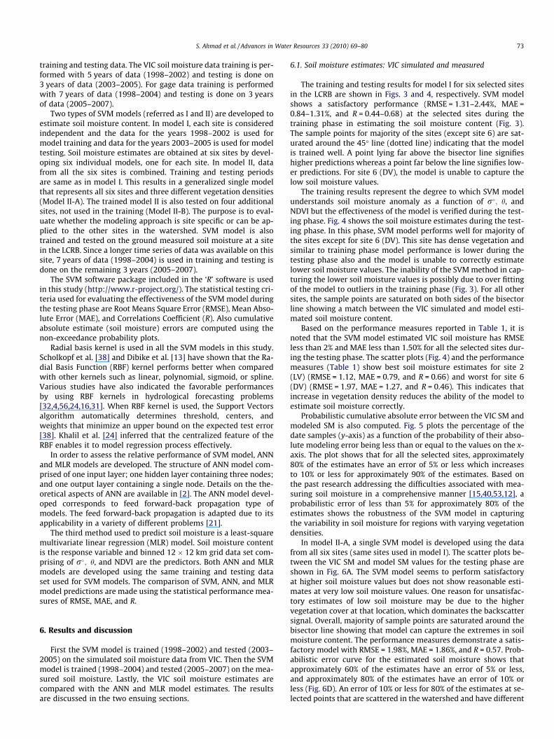
The training and testing results for model I for six selected sitesin the LCRB are shown in Figs. 3 and 4, respectively. SVM modelshows a satisfactory performance (RMSE = 1.31–2.44%, MAE =0.84–1.31%, and R = 0.44–0.68) at the selected sites during thetraining phase in estimating the soil moisture content (Fig. 3).The sample points for majority of the sites (except site 6) are sat-urated around the 45� line (dotted line) indicating that the modelis trained well. A point lying far above the bisector line signifieshigher predictions whereas a point far below the line signifies low-er predictions. For site 6 (DV), the model is unable to capture thelow soil moisture values.

The training results represent the degree to which SVM modelunderstands soil moisture anomaly as a function of r�; h, andNDVI but the effectiveness of the model is verified during the test-ing phase. Fig. 4 shows the soil moisture estimates during the test-ing phase. In this phase, SVM model performs well for majority ofthe sites except for site 6 (DV). This site has dense vegetation andsimilar to training phase model performance is lower during thetesting phase also and the model is unable to correctly estimatelower soil moisture values. The inability of the SVM method in cap-turing the lower soil moisture values is possibly due to over fittingof the model to outliers in the training phase (Fig. 3). For all othersites, the sample points are saturated on both sides of the bisectorline showing a match between the VIC simulated and model esti-mated soil moisture content.

Based on the performance measures reported in Table 1, it isnoted that the SVM model estimated VIC soil moisture has RMSEless than 2% and MAE less than 1.50% for all the selected sites dur-ing the testing phase. The scatter plots (Fig. 4) and the performancemeasures (Table 1) show best soil moisture estimates for site 2(LV) (RMSE = 1.12, MAE = 0.79, and R = 0.66) and worst for site 6(DV) (RMSE = 1.97, MAE = 1.27, and R = 0.46). This indicates thatincrease in vegetation density reduces the ability of the model toestimate soil moisture correctly.

Probabilistic cumulative absolute error between the VIC SM andmodeled SM is also computed. Fig. 5 plots the percentage of thedate samples (y-axis) as a function of the probability of their abso-lute modeling error being less than or equal to the values on the x-axis. The plot shows that for all the selected sites, approximately80% of the estimates have an error of 5% or less which increasesto 10% or less for approximately 90% of the estimates. Based onthe past research addressing the difficulties associated with mea-suring soil moisture in a comprehensive manner [15,40,53,12], aprobabilistic error of less than 5% for approximately 80% of theestimates shows the robustness of the SVM model in capturingthe variability in soil moisture for regions with varying vegetationdensities.

In model II-A, a single SVM model is developed using the datafrom all six sites (same sites used in model I). The scatter plots be-tween the VIC SM and model SM values for the testing phase areshown in Fig. 6A. The SVM model seems to perform satisfactoryat higher soil moisture values but does not show reasonable esti-mates at very low soil moisture values. One reason for unsatisfac-tory estimates of low soil moisture may be due to the highervegetation cover at that location, which dominates the backscattersignal. Overall, majority of sample points are saturated around thebisector line showing that model can capture the extremes in soilmoisture content. The performance measures demonstrate a satis-factory model with RMSE = 1.98%, MAE = 1.86%, and R = 0.57. Prob-abilistic error curve for the estimated soil moisture shows thatapproximately 60% of the estimates have an error of 5% or less,and approximately 80% of the estimates have an error of 10% orless (Fig. 6D). An error of 10% or less for 80% of the estimates at se-lected points that are scattered in the watershed and have different

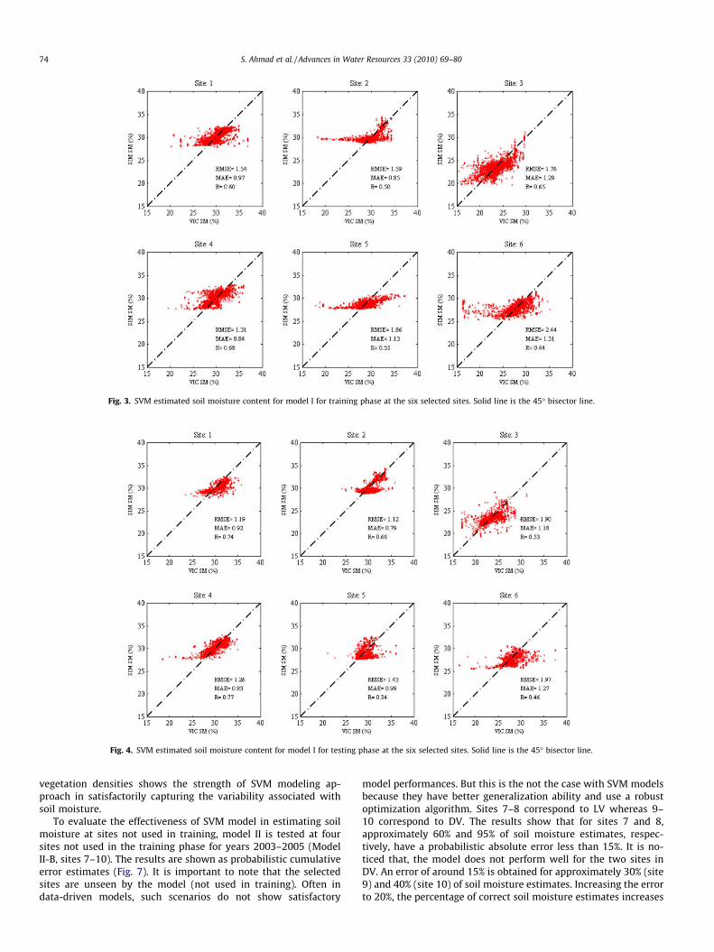
Fig. 3. SVM estimated soil moisture content for model I for training phase at the six selected sites. Solid line is the 45� bisector line.

Fig. 4. SVM estimated soil moisture content for model I for testing phase at the six selected sites. Solid line is the 45� bisector line.

74 S. Ahmad et al. / Advances in Water Resources 33 (2010) 69–80

vegetation densities shows the strength of SVM modeling ap-proach in satisfactorily capturing the variability associated withsoil moisture.

To evaluate the effectiveness of SVM model in estimating soilmoisture at sites not used in training, model II is tested at foursites not used in the training phase for years 2003–2005 (ModelII-B, sites 7–10). The results are shown as probabilistic cumulativeerror estimates (Fig. 7). It is important to note that the selectedsites are unseen by the model (not used in training). Often indata-driven models, such scenarios do not show satisfactory

model performances. But this is the not the case with SVM modelsbecause they have better generalization ability and use a robustoptimization algorithm. Sites 7–8 correspond to LV whereas 9–10 correspond to DV. The results show that for sites 7 and 8,approximately 60% and 95% of soil moisture estimates, respec-tively, have a probabilistic absolute error less than 15%. It is no-ticed that, the model does not perform well for the two sites inDV. An error of around 15% is obtained for approximately 30% (site9) and 40% (site 10) of soil moisture estimates. Increasing the errorto 20%, the percentage of correct soil moisture estimates increases

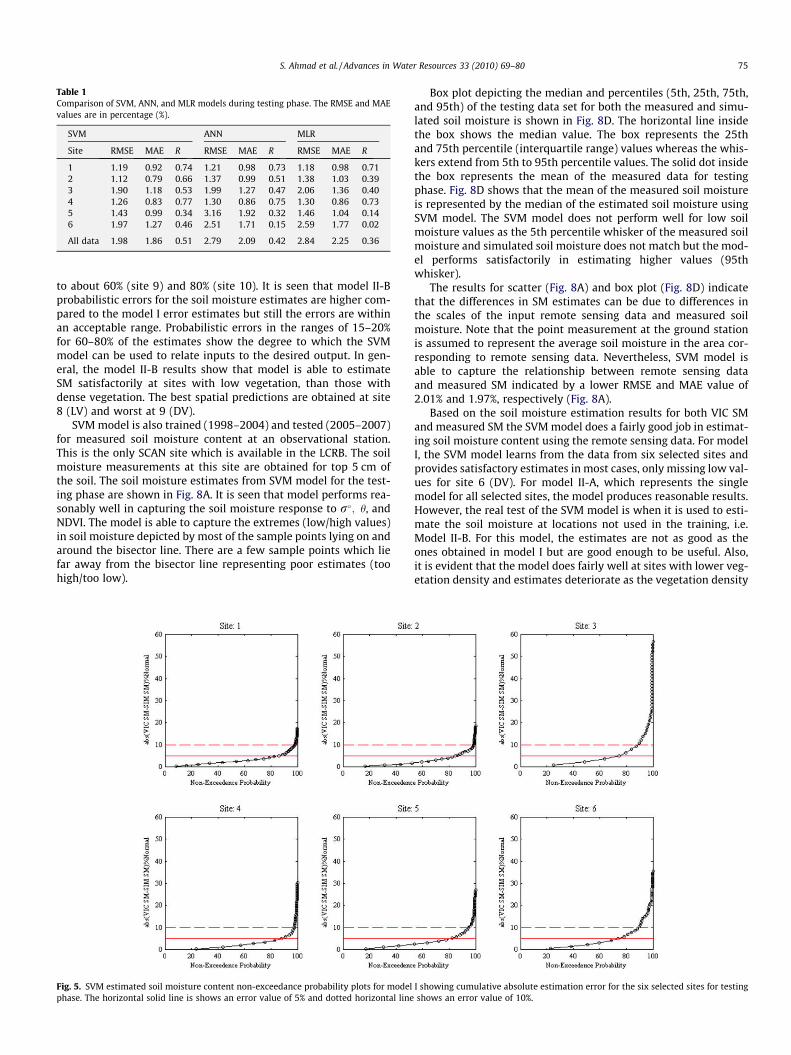
Table 1Comparison of SVM, ANN, and MLR models during testing phase. The RMSE and MAEvalues are in percentage (%).

SVM ANN MLR

Site RMSE MAE R RMSE MAE R RMSE MAE R

1 1.19 0.92 0.74 1.21 0.98 0.73 1.18 0.98 0.712 1.12 0.79 0.66 1.37 0.99 0.51 1.38 1.03 0.393 1.90 1.18 0.53 1.99 1.27 0.47 2.06 1.36 0.404 1.26 0.83 0.77 1.30 0.86 0.75 1.30 0.86 0.735 1.43 0.99 0.34 3.16 1.92 0.32 1.46 1.04 0.146 1.97 1.27 0.46 2.51 1.71 0.15 2.59 1.77 0.02

All data 1.98 1.86 0.51 2.79 2.09 0.42 2.84 2.25 0.36

S. Ahmad et al. / Advances in Water Resources 33 (2010) 69–80 75

to about 60% (site 9) and 80% (site 10). It is seen that model II-Bprobabilistic errors for the soil moisture estimates are higher com-pared to the model I error estimates but still the errors are withinan acceptable range. Probabilistic errors in the ranges of 15–20%for 60–80% of the estimates show the degree to which the SVMmodel can be used to relate inputs to the desired output. In gen-eral, the model II-B results show that model is able to estimateSM satisfactorily at sites with low vegetation, than those withdense vegetation. The best spatial predictions are obtained at site8 (LV) and worst at 9 (DV).

SVM model is also trained (1998–2004) and tested (2005–2007)for measured soil moisture content at an observational station.This is the only SCAN site which is available in the LCRB. The soilmoisture measurements at this site are obtained for top 5 cm ofthe soil. The soil moisture estimates from SVM model for the test-ing phase are shown in Fig. 8A. It is seen that model performs rea-sonably well in capturing the soil moisture response to r�; h, andNDVI. The model is able to capture the extremes (low/high values)in soil moisture depicted by most of the sample points lying on andaround the bisector line. There are a few sample points which liefar away from the bisector line representing poor estimates (toohigh/too low).

Fig. 5. SVM estimated soil moisture content non-exceedance probability plots for modelphase. The horizontal solid line is shows an error value of 5% and dotted horizontal line

Box plot depicting the median and percentiles (5th, 25th, 75th,and 95th) of the testing data set for both the measured and simu-lated soil moisture is shown in Fig. 8D. The horizontal line insidethe box shows the median value. The box represents the 25thand 75th percentile (interquartile range) values whereas the whis-kers extend from 5th to 95th percentile values. The solid dot insidethe box represents the mean of the measured data for testingphase. Fig. 8D shows that the mean of the measured soil moistureis represented by the median of the estimated soil moisture usingSVM model. The SVM model does not perform well for low soilmoisture values as the 5th percentile whisker of the measured soilmoisture and simulated soil moisture does not match but the mod-el performs satisfactorily in estimating higher values (95thwhisker).

The results for scatter (Fig. 8A) and box plot (Fig. 8D) indicatethat the differences in SM estimates can be due to differences inthe scales of the input remote sensing data and measured soilmoisture. Note that the point measurement at the ground stationis assumed to represent the average soil moisture in the area cor-responding to remote sensing data. Nevertheless, SVM model isable to capture the relationship between remote sensing dataand measured SM indicated by a lower RMSE and MAE value of2.01% and 1.97%, respectively (Fig. 8A).

Based on the soil moisture estimation results for both VIC SMand measured SM the SVM model does a fairly good job in estimat-ing soil moisture content using the remote sensing data. For modelI, the SVM model learns from the data from six selected sites andprovides satisfactory estimates in most cases, only missing low val-ues for site 6 (DV). For model II-A, which represents the singlemodel for all selected sites, the model produces reasonable results.However, the real test of the SVM model is when it is used to esti-mate the soil moisture at locations not used in the training, i.e.Model II-B. For this model, the estimates are not as good as theones obtained in model I but are good enough to be useful. Also,it is evident that the model does fairly well at sites with lower veg-etation density and estimates deteriorate as the vegetation density

I showing cumulative absolute estimation error for the six selected sites for testingshows an error value of 10%.

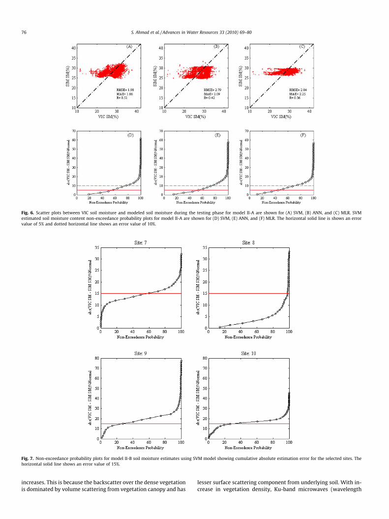
Fig. 6. Scatter plots between VIC soil moisture and modeled soil moisture during the testing phase for model II-A are shown for (A) SVM, (B) ANN, and (C) MLR. SVMestimated soil moisture content non-exceedance probability plots for model II-A are shown for (D) SVM, (E) ANN, and (F) MLR. The horizontal solid line is shows an errorvalue of 5% and dotted horizontal line shows an error value of 10%.

Fig. 7. Non-exceedance probability plots for model II-B soil moisture estimates using SVM model showing cumulative absolute estimation error for the selected sites. Thehorizontal solid line shows an error value of 15%.

76 S. Ahmad et al. / Advances in Water Resources 33 (2010) 69–80

increases. This is because the backscatter over the dense vegetationis dominated by volume scattering from vegetation canopy and has

lesser surface scattering component from underlying soil. With in-crease in vegetation density, Ku-band microwaves (wavelength

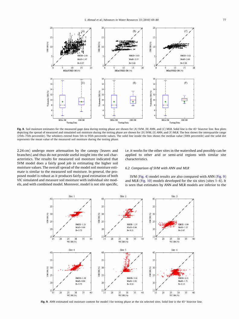
Fig. 8. Soil moisture estimates for the measured gage data during testing phase are shown for (A) SVM, (B) ANN, and (C) MLR. Solid line is the 45� bisector line. Box plotsdepicting the spread of measured and simulated soil moisture during the testing phase are shown for (D) SVM, (E) ANN, and (F) MLR. The box shows the interquartile range(25th–75th percentile). The whiskers extend from 5th to 95th percentile values. The solid line inside the box shows the median value (50th percentile) and the solid dotrepresents the mean value of the measured soil moisture during the testing phase.

S. Ahmad et al. / Advances in Water Resources 33 (2010) 69–80 77

2.24 cm) undergo more attenuation by the canopy (leaves andbranches) and thus do not provide useful insight into the soil char-acteristics. The results for measured soil moisture indicated thatSVM model does a fairly good job in estimating the higher soilmoisture values. The overall spread of the model soil moisture esti-mate is similar to the measured soil moisture. In general, the pro-posed model is robust as it produces fairly good estimation of bothVIC simulated and measure soil moisture with individual site mod-els, and with combined model. Moreover, model is not site specific,

Fig. 9. ANN estimated soil moisture content for model I for testing p

i.e. it works for the other sites in the watershed and possibly can beapplied to other arid or semi-arid regions with similar sitecharacteristics.

6.2. Comparison of SVM with ANN and MLR

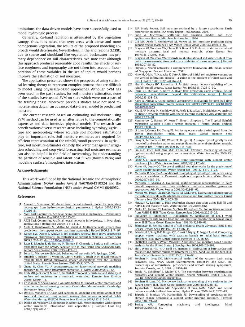
SVM (Fig. 4) model results are also compared with ANN (Fig. 9)and MLR (Fig. 10) models developed for the six sites (sites 1–6). Itis seen that estimates by ANN and MLR models are inferior to the

hase at the six selected sites. Solid line is the 45� bisector line.

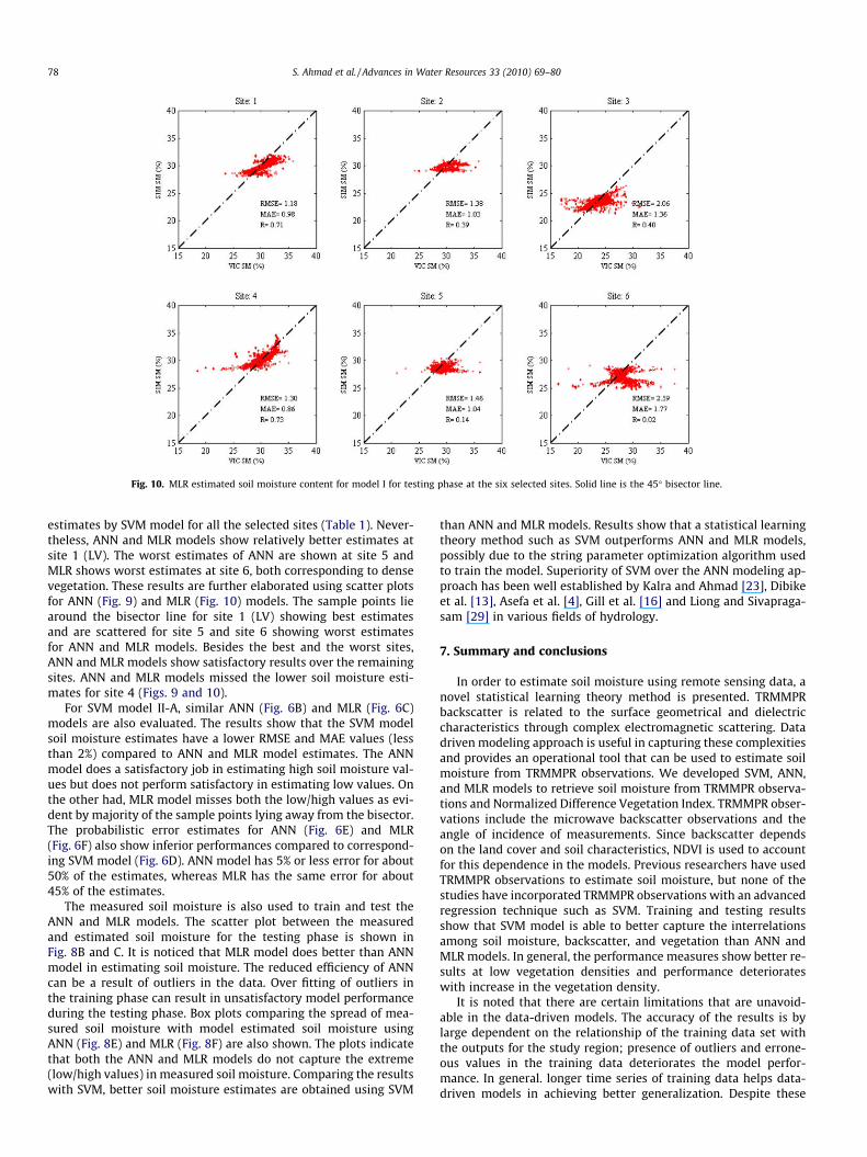
Fig. 10. MLR estimated soil moisture content for model I for testing phase at the six selected sites. Solid line is the 45� bisector line.

78 S. Ahmad et al. / Advances in Water Resources 33 (2010) 69–80

estimates by SVM model for all the selected sites (Table 1). Never-theless, ANN and MLR models show relatively better estimates atsite 1 (LV). The worst estimates of ANN are shown at site 5 andMLR shows worst estimates at site 6, both corresponding to densevegetation. These results are further elaborated using scatter plotsfor ANN (Fig. 9) and MLR (Fig. 10) models. The sample points liearound the bisector line for site 1 (LV) showing best estimatesand are scattered for site 5 and site 6 showing worst estimatesfor ANN and MLR models. Besides the best and the worst sites,ANN and MLR models show satisfactory results over the remainingsites. ANN and MLR models missed the lower soil moisture esti-mates for site 4 (Figs. 9 and 10).

For SVM model II-A, similar ANN (Fig. 6B) and MLR (Fig. 6C)models are also evaluated. The results show that the SVM modelsoil moisture estimates have a lower RMSE and MAE values (lessthan 2%) compared to ANN and MLR model estimates. The ANNmodel does a satisfactory job in estimating high soil moisture val-ues but does not perform satisfactory in estimating low values. Onthe other had, MLR model misses both the low/high values as evi-dent by majority of the sample points lying away from the bisector.The probabilistic error estimates for ANN (Fig. 6E) and MLR(Fig. 6F) also show inferior performances compared to correspond-ing SVM model (Fig. 6D). ANN model has 5% or less error for about50% of the estimates, whereas MLR has the same error for about45% of the estimates.

The measured soil moisture is also used to train and test theANN and MLR models. The scatter plot between the measuredand estimated soil moisture for the testing phase is shown inFig. 8B and C. It is noticed that MLR model does better than ANNmodel in estimating soil moisture. The reduced efficiency of ANNcan be a result of outliers in the data. Over fitting of outliers inthe training phase can result in unsatisfactory model performanceduring the testing phase. Box plots comparing the spread of mea-sured soil moisture with model estimated soil moisture usingANN (Fig. 8E) and MLR (Fig. 8F) are also shown. The plots indicatethat both the ANN and MLR models do not capture the extreme(low/high values) in measured soil moisture. Comparing the resultswith SVM, better soil moisture estimates are obtained using SVM

than ANN and MLR models. Results show that a statistical learningtheory method such as SVM outperforms ANN and MLR models,possibly due to the string parameter optimization algorithm usedto train the model. Superiority of SVM over the ANN modeling ap-proach has been well established by Kalra and Ahmad [23], Dibikeet al. [13], Asefa et al. [4], Gill et al. [16] and Liong and Sivapraga-sam [29] in various fields of hydrology.

7. Summary and conclusions

In order to estimate soil moisture using remote sensing data, anovel statistical learning theory method is presented. TRMMPRbackscatter is related to the surface geometrical and dielectriccharacteristics through complex electromagnetic scattering. Datadriven modeling approach is useful in capturing these complexitiesand provides an operational tool that can be used to estimate soilmoisture from TRMMPR observations. We developed SVM, ANN,and MLR models to retrieve soil moisture from TRMMPR observa-tions and Normalized Difference Vegetation Index. TRMMPR obser-vations include the microwave backscatter observations and theangle of incidence of measurements. Since backscatter dependson the land cover and soil characteristics, NDVI is used to accountfor this dependence in the models. Previous researchers have usedTRMMPR observations to estimate soil moisture, but none of thestudies have incorporated TRMMPR observations with an advancedregression technique such as SVM. Training and testing resultsshow that SVM model is able to better capture the interrelationsamong soil moisture, backscatter, and vegetation than ANN andMLR models. In general, the performance measures show better re-sults at low vegetation densities and performance deteriorateswith increase in the vegetation density.

It is noted that there are certain limitations that are unavoid-able in the data-driven models. The accuracy of the results is bylarge dependent on the relationship of the training data set withthe outputs for the study region; presence of outliers and errone-ous values in the training data deteriorates the model perfor-mance. In general. longer time series of training data helps data-driven models in achieving better generalization. Despite these

S. Ahmad et al. / Advances in Water Resources 33 (2010) 69–80 79

limitations, the data-driven models have been successfully used tomodel hydrologic process.

Generally, Ku-band radiation is attenuated by the vegetationcanopy, thus, it is noted that over areas with dense and morehomogenous vegetation, the results of the proposed modeling ap-proach would deteriorate. Nevertheless, in the arid regions (LCRB),due to sparse and shrubland like vegetation, backscatter has pri-mary dependence on soil characteristics. We note that althoughthis approach produces reasonably good results, the effects of sur-face roughness and topography are not taken into account. Incor-poration of these variables in the set of inputs would perhapsimprove the estimation of soil moisture.

The application presented shows the prospects of using statisti-cal learning theory to represent complex process that are difficultto model using physically-based approaches. Although SVM hasbeen used, in the past studies, for soil moisture estimation, noneof the studies have tested SVM on sites which were not a part ofthe training phase. Moreover, previous studies have not used re-mote sensing data in an advanced data-driven model to predict soilmoisture.

The current research based on estimating soil moisture usingSVM method can be used as an alternative to the computationallyexpensive and data intensive physical models. The research canbenefit various diverse research areas including hydrology, agricul-ture and meteorology where accurate soil moisture estimationsplay an important role. Soil moisture estimates are required forefficient representation of the rainfall/runoff processes. In agricul-ture, soil moisture estimates can help the water managers in irriga-tion scheduling and crop yield forecasting. Soil moisture estimatescan also be helpful in the field of meteorology for understandingthe partition of sensible and latent heat fluxes (Bowen Ratio) andmodeling surface/atmospheric interactions.

Acknowledgments

This work was funded by the National Oceanic and AtmosphericAdministration (NOAA) under Award NA070AR4310324 and theNational Science Foundation (NSF) under Award CMMI-0846952.

References

[1] Ahmad S, Simonovic SP. An artificial neural network model for generatinghydrograph from hydro-meteorological parameters. J Hydrol 2005;315(1–4):236–51.

[2] ASCE Task Committee. Artificial neural networks in hydrology. I: Preliminaryconcepts. J Hydrol Eng 2000;5(2):115–23.

[3] ASCE Task Committee. Artificial neural networks in hydrology. II: Hydrologicapplications. J Hydrol Eng 2000;5(2):124–37.

[4] Asefa T, Kemblowski M, McKee M, Khalil A. Multi-time scale stream flowpredictions: the support vector machines approach. J Hydrol 2006;318:7–16.

[5] Barrett BW, Dwyer E, Whelan P. Soil moisture retrieval from active spacebornemicrowave observations: an evaluation of current techniques. Remote Sens2009;1:210–42. doi:10.3390/rs1030210.

[6] Baup F, Mougin E, de Rosney P, Timouk F, Chenerie I. Surface soil moistureestimation over the AMMA Sahelian site in Mali using ENVISAT/ASAR data.Remote Sens Environ 2007;109(4):473–81.

[7] Behari J. Microwave dielectric behaviour of wet soils. NY: Springer; 2005.[8] Bindlish R, Jackson TJ, Wood EF, Gao H, Starks P, Bosch D, et al. Soil moisture

estimate from TRMM microwave imager observations over the SouthernUnited States. Remote Sens Environ 2003;85(4):507–15.

[9] Chang FJ, Chen YC. A counterpropagation fuzzy-neural network modelingapproach to real time streamflow prediction. J Hydrol 2001;245:153–64.

[10] Cosh MH, Jackson TJ, Moran S, Bindlish R. Temporal persistence and stability ofsurface soil moisture in a semi-arid watershed. Remote Sens Environ2008;112:304–13.

[11] Cristianini N, Shaw-Taylor J. An introduction to support vector machines andother kernel based learning methods. Cambridge, Massachusetts: CambridgeUniversity Press; 2000.

[12] Das NN, Mohanty BP, Cosh MH, Jackson TJ. Modeling and assimilation of rootzone soil moisture using remote sensing observations in Walnut GulchWatershed during SMEX04. Remote Sens Environ 2008;112:415–29.

[13] Dibike YB, Velickov S, Solomatine D, Abbott MB. Model induction with supportvector machines: introduction and application. J Comput Civil Eng2001;15(3):208–16.

[14] ESA Study Report. Soil moisture retrieval by a future space-borne Earthobservation mission. ESA Study Report 14662/00/NL, 2004.

[15] Fung A. Microwave scattering and emission models and theirapplications. Boston, MA: Artech House Inc.; 1994.

[16] Gill MK, Asefa T, Kemblowski M, McKee M. Soil moisture prediction usingsupport vector machines. J Am Water Resour Assoc 2006;42(4):1033–46.

[17] Grayson RB, Western AW, Chiew FHS, Bloschl G. Preferred states in spatial soilmoisture patterns: local and nonlocal controls. Water Resour Res1997;33(12):2897–908.

[18] Grayson RB, Western AW. Towards areal estimation of soil water content frompoint measurements: time and space stability of mean response. J Hydrol1998;207:68–82.

[19] Haykin S. Neural networks: a comprehensive foundation. 4th Indian Reprinted. Singapore: Pearson Education; 2003.

[20] Hino M, Odaka Y, Nadaoka K, Sato A. Effect of initial soil moisture content onthe vertical infiltration process – a guide to the problem of runoff-ratio andloss. J Hydrol 1988;102(1–4):267–84.

[21] Hsu K-I, Gupta HV, Sorooshian S. Artificial neural network modeling of therainfall–runoff process. Water Resour Res 1995;31(10):2517–30.

[22] Imrie CE, Durucan S, Korre A. River flow prediction using artificial neuralnetworks: generalization beyond the calibration range. J Hydrol2000;233:138–53.

[23] Kalra A, Ahmad S. Using oceanic–atmospheric oscillations for long lead timestreamflow forecasting. Water Resour Res 2009;45:W03413. doi:10,1029/2008WR006855.

[24] Khalil AF, McKee M, Kemblowski M, Asefa T, Bastidas L. Multiobjective analysisof chaotic dynamic systems with sparse learning machines. Adv Water Resour2006;29:72–88.

[25] Kummerow C, Barnes W, Kozu T, Shiue J, Simpson J. The Tropical RainfallMeasuring Mission (TRMM) sensor package. J Atmos Ocean Technol1998;15:808–16.

[26] Li L, Im E, Connor LN, Chang PS. Retrieving ocean surface wind speed from theTRMM precipitation radar. IEEE Trans Geosci Remote Sens2004;42(6):1271–82.

[27] Liang X, Lettenmaier DP, Wood EF, Burges SJ. A simple hydrologically basedmodel of land-surface water and energy fluxes for general-circulation models.J Geophys Res – Atmos 1994;99(D7):15–428.

[28] Lin G-F, Chen G-R, Wu M-C, Chou Y-C. Effective forecasting of hourlytyphoon rainfall using support vector machines. Water Resour Res 2009;45:W08440.

[29] Liong S-Y, Sivapragasam C. Flood stage forecasting with support vectormachines. J Am Water Resour Assoc 2002;38(1):173–86.

[30] Maier HR, Dandy GC. The use of artificial neural networks for the prediction ofwater quality parameters. Water Resour Res 1996;32(4):1013–22.

[31] Mehrotra R, Sharma A. Conditional resampling of hydrologic time series usingpredictor variables: a K-nearest neighbour approach. Adv Water Resour2006;29(7):987–99.

[32] Mehrotra R, Sharma A. Evaluating spatio-temporal representation in dailyrainfall sequences from three stochastic multi-site weather generationapproaches. Adv Water Resour 2009;32(6):948–62.

[33] Moran MS, Peters-Lidard CD, Watts JM, McElroy S. Estimating soil moisture atthe watershed scale with satellite-based radar and land surface models. CanadJ Remote Sens 2004;30(5):805–26.

[34] Narayan U, Lakshmi V. High resolution change detection using TMI-PR andAMSR-E soil moisture data. Water Resour Res 2008;44(6).

[35] Njoku EG, Jackson TJ, Lakshmi V, Chan TK, Nghiem SV. Soil moisture retrievalfrom AMSR-E. IEEE Trans Geosci Remote Sens 2003;41(2):215–29.

[36] Pulliainen JT, Manninen T, Hallikainen M. Application of ERS-1 windscatterometer data to soil frost and soil moisture monitoring in Boreal forestzone. IEEE Trans Geosci Remote Sens 1998;36(3):849–63.

[37] Schmugge TJ. Remote sensing of soil moisture: recent advances. IEEE TransGeosci Remote Sens 1983;GE-21(3):336–44.

[38] Scholkopf B, Sung K-K, Burges CJC, Girosi F, Niyogi P, Poggio T, et al. Comparingsupport vector machines with gaussian kernels to radial basis functionclassifiers. IEEE Trans Signal Process 1997;45(11):2758–65.

[39] Sheffield J, Goteti G, Wen F, Wood EF. A simulated soil moisture based droughtanalysis for the United States. J Geophys Res 2004;109:D24108.

[40] Shi J, Wang A, Hsu Y, O’ Neill PE, Engman ET. Estimation of bare surface soilmoisture and surface roughness parameter using L-band SAR image data. IEEETrans Geosci Remote Sens 1997;35(5):1254–66.

[41] Stephen H, Long DG. Multi-spectral analysis of the Amazon basin usingSeawinds, ERS, NASA, Seasat Scatterometer, TRMM-PR and SSM/I. In:Proceedings of international geosciences and remote sensing symposium,Toronto, Canada, vol. 5, 2002. p. 2808–10.

[42] Smola AJ, Schölkopf B, Muller K-R. The connection between regularizationoperators and support vector kernels. Neural Networks 1998;11:637–49.doi:10.1016/S0893-6080(98)00032-X.

[43] Stephen H, Long DG. Microwave backscatter modeling of erg surfaces in theSahara desert. IEEE Trans Geosci Remote Sens 2005;43(2):238–47.

[44] Tigsanchali T, Gautam MR. Application of tank, NAM, ARMA, and neuralnetwork models to flood forecasting. Hydrol Process 2000;14(4):2473–87.

[45] Tripathi S, Srinivas VV, Nanjundiah RS. Downscaling of precipitation forclimate change scenarios: a support vector machine approach. J Hydrol2006;330:621–40.

[46] Turing AM. Computing machinery and intelligence. Mind1950;59(236):433–60.

80 S. Ahmad et al. / Advances in Water Resources 33 (2010) 69–80

[47] Twarakavi NKC, Mishra D, Bandopadhyay S. Prediction of arsenic in bedrockderived stream sediments at a gold mine site under conditions of sparse data.Nat Resour Res 2006;15(1):15–26.

[48] Ulaby F, Moore R, Fung A. Microwave remote sensing: active and passive, vol.3. Norwood, MA: Artech House, Inc.; 1982.

[49] Vapnik V. The nature of statistical learning theory. New York: Springer; 1995.[50] Vapnik V. Statistical learning theory. New York: Wiley; 1998.[51] Vapnik V, Cherkassky V. On the uniform convergence of relative frequencies of

events to their probabilities. Theory Probab Appl 1971;16: 264–80.[52] Wagner W, Bloschl D, Pampaloni J-C, Bizzarri B, Wigneron J-P, Kerr Y.

Operational readiness of microwave remote sensing of soil moisture forhydrologic applications. Nordic Hydrol 2007;38(1):1–20.

[53] Wen J, Su Z, Ma Y. Determination of land surface temperature and soilmoisture from tropical rainfall measuring mission/microwave imager remotesensing data. J Geophys Res 2003;108(D2):805–26.

[54] Western AW, Grayson RB, Bloschl G. Scaling of soil moisture: a hydrologicperspective. Ann Rev Earth Planet Sci 2002;30:149–80.

[55] Woodhouse IH, Hoekman DH. A model-based determination of soil moisturetrends in Spain with ERS-scattermeter. IEEE Trans Geosci Remote Sens2000;38(4):1783–93.

[56] Yu X, Liong S-Y. Forecasting of hydrologic time series with ridge regression infeature space. J Hydrol 2007;332:290–302.

[57] Zealand CM, Burn DH, Simonovic SP. Short term streamflow forecasting usingartificial neural networks. J Hydrol 1999;214:32–48.