Centre for Budget and Policy Studies i Estimating Multiplier Effect of Social Sector Expenditure in Karnataka An exploration through the Input – Output table and Social Accounting Matrix December 2020 Supporting Agency: The Department of Finance, Government of Karnataka

Welcome message from author
This document is posted to help you gain knowledge. Please leave a comment to let me know what you think about it! Share it to your friends and learn new things together.
Transcript
Centre for Budget and Policy Studies i
Estimating Multiplier Effect of Social
Sector Expenditure in Karnataka
An exploration through the Input – Output table and Social
Accounting Matrix
December 2020
Supporting Agency: The Department of Finance, Government of
Karnataka

Estimating Multiplier Effect of Social Sector Expenditure in Karnataka
Centre for Budget and Policy Studies ii
'Draft circulated for comments'
Estimating Multiplier Effect of Social Sector Expenditure in Karnataka
Centre for Budget and Policy Studies iii
This paper can be quoted in part, with the full citation. Suggested citation: Achala S. Yareseeme*, Apurva K.H*1, Jyotsna Jha, Archana Purohit, (2021),
Estimating Multiplier Effect of Social Sector Expenditure in Karnataka
An exploration through the Input – Output table and Social Accounting Matrix.
Centre for Budget and Policy Studies Supporting Agency: The Department of Finance, Government of Karnataka.
1* These authors’ have contributed equally
Estimating Multiplier Effect of Social Sector Expenditure in Karnataka
Centre for Budget and Policy Studies iv
Table of Contents
Acknowledgements .................................................................................................................... 1
List of Tables ............................................................................................................................. 2
List of Figures ............................................................................................................................ 3
List of Abbreviations ................................................................................................................. 4
Chapter 1. Introduction .............................................................................................................. 5
Chapter 2. Multiplier: Concept, Context, & Types .................................................................... 7
2.1 Concept & Context ........................................................................................................... 7
2.2 Types of Multipliers ......................................................................................................... 8
2.3 Review of Literature......................................................................................................... 9
2.4 Methods used to estimate Multiplier .............................................................................. 13
2.4.1 Input-Output Models ............................................................................................... 13
2.4.2 Social Accounting Matrix ........................................................................................ 15
Chapter 3. Construction of IOTT and SAM for Karnataka 2013-14 ...................................... 19
3.1 Background .................................................................................................................... 19
3.2 Mapping of the Karnataka SDP sectors against India’s I-O Table ................................ 21
3.3 Process towards the construction of IOTT and SAM for Karnataka 2013-14 ............... 23
3.3.1 Gross Value of Output (GVO) ................................................................................. 23
3.3.2 Estimation of Intermediate consumption/use matrix ............................................... 23
3.3.3 Final Demand Components ..................................................................................... 24
3.3.4 Net Indirect Taxes ................................................................................................... 24
3.3.5 Construction of SAM for Karnataka ....................................................................... 24
Chapter 4. Analysis and Discussions ....................................................................................... 26
4.1 Components of Aggregate Demand ............................................................................... 26
4.2 Decomposition of Gross Value Added........................................................................... 27
4.3 Distribution of Output Disposition and Distribution of Inputs ...................................... 28
4.4 PFCE Distribution across Occupational Households ..................................................... 30
4.5 Factor Incomes to Households ....................................................................................... 32
4.6 Factor Incomes to Private Corporate and Public Sector Enterprises ............................. 33
4.7 Sectoral Investment in Karnataka .................................................................................. 33
4.8 Savings ........................................................................................................................... 35
4.9 Direct and Indirect Tax Share ........................................................................................ 35
4.10 Analyses of Multipliers ................................................................................................ 35
Estimating Multiplier Effect of Social Sector Expenditure in Karnataka
Centre for Budget and Policy Studies v
4.10.1 Linkages................................................................................................................. 35
4.10.2 Own Multipliers ..................................................................................................... 37
4.10.3 Output Multiplier SAM and IOTT ........................................................................ 38
4.10.4 Household Income Multiplier SAM ...................................................................... 39
4.10.5 Primary Input multipliers....................................................................................... 39
4.10.6 HH Income Multiplier across Households ............................................................ 40
4.10.7 Full Income Multipliers ......................................................................................... 41
4.10.8 Comparison of SAM and IOTT Multipliers .......................................................... 42
4.11 Policy Conclusions ....................................................................................................... 44
References ................................................................................................................................ 46
Annexures ................................................................................................................................ 52
Annexure 1: The Accounts of Social Accounting Matrix (SAM) ....................................... 52
Annexure 2: Estimation of Input Structures:........................................................................ 54
Annexure 3: Computation of Final Demand Components ................................................... 58
Annexure 4: Net Indirect Taxes ........................................................................................... 75
Annexure 5: Construction of Components of Social Accounting Matrix ............................ 79
Annexure 6: Tools to estimate Multiplier ............................................................................ 87
Annexure 7: Leontief Inverse Matrix to calculate Multiplier .............................................. 89
Annexure 8: List of Universities and Hospitals ................................................................... 90
Annexure 9: Input-Output Table for Karnataka 2013-14 (In Excel Sheets) ........................ 90
Annexure 10: Social Accounting Matrix for Karnataka 2013-14 (In Excel Sheets) ........... 90
Notes ........................................................................................................................................ 91
Notes ........................................................................................................................................ 92
Notes ........................................................................................................................................ 93
Notes ........................................................................................................................................ 94
Centre for Budget and Policy Studies 1
Acknowledgements
The long enduring process of completing this project would never be complete without the
valuable support of many people. First, we would like to express our immense gratitude to ISN
Prasad, Additional Chief Secretary, Department of Finance, Government of Karnataka for
showing an interest and approving the funding for this project. It is important for such a
research to be supported through public funds. He and his team have also been extremely
supportive in providing us with guidance and directions in the process of data collection.
We further would like to mention the support received by Dr. Shalini Rajneesh, Principal
Secretary, Department of Planning, Programme Monitoring and Statistics Department,
Government of Karnataka for granting permission and extending help in accessing crucial data
for this work. Mr. Narasimha Phani, Joint Director, Directorate of Economics and Statistics,
Govt. of Karnataka, provided continuous feedback and inputs, which helped us fine tune our
work to its current stature. Further, we would like to extend our appreciation to Dr. Ekroop
Kaur, Secretary, Budget & Resources in the Department of Finance, Government of Karnataka,
Mr. Purushottam Singh from the Department of Finance, Government of Karnataka and their
team, for all the administrative work and timely help in accessing other public offices.
Our Advisory Board comprising of Ganesh Kumar, Anushree Sinha, Arjun Jayadev and Vinod
Vyasulu provided us with initial guidance to kick start the work. Mr. M R Saluja also made
himself available for feedback at a crucial juncture which helped us review and modify our
methodology. We especially thank Dr. A. Indira, our Board member, for her review of the
report. We would like to specially mention our thanks to Prof. Vinod Vyasulu, President, CBPS
Board for providing us with all the networks and resources.
We thank all the staff of Administrative Departments, Public Sector Undertakings and other
Public Offices of the Government of Karnataka for providing us with the required data as and
when we approached them. We express our gratitude to our colleagues for all the questions and
conversations that were put at us which helped us deepen the insight towards this work. Mr.
Madhusudhan Rao B V and Mr. Shreekanth Mahendiran deserve special mention for their
inputs to the proposal. We sincerely thank our CBPS Administration Team, Mr Ramesh K.A,
Ms. Vanaja S and Ms. Usha P.V for facilitating all the requirements for us.
-The Research Team, CBPS
Research Team at Centre for Budget and Policy Studies (CBPS), Bangalore:
Achala S. Yareseeme.,
Apurva K.H.,
Jyotsna Jha.,
Archana Purohit.
Estimating Multiplier Effect of Social Sector Expenditure in Karnataka
Centre for Budget and Policy Studies 2
List of Tables
Table 3.1: Concordance Matrix of India I-O Sectors with Karnataka SDP Sectors ................ 22
Table 4.1: Share of Aggregate Demand Components in Final GSDP (2013-14)……………27
Table 4.2: Distribution of PFCE across sectors across household categories ......................... 32
Table 4.3: Sectoral share of Investment ................................................................................... 34
Table 4.4: Linkage coefficient across sectors .......................................................................... 36
Table 4.5: Own IOTT and SAM Multipliers ........................................................................... 37
Table 4.6: Output Multipliers for IOTT and SAM .................................................................. 38
Table 4.7: Household Income Multipliers .............................................................................. 39
Table 4.8: Primary Input Multipliers ....................................................................................... 40
Table 4.9: Income Multipliers by Household Groups ............................................................. 41
Table 4.10: Full Income Multipliers by HH Groups................................................................ 41
Table 4.11: Key sector identification based on multiplier values ............................................ 43
Table A3.1: Classification of budget expenditure items into different heads ………………..63
Table A3.2: Summary of Gram Panchayat Accounts .............................................................. 66
Table A4. 1: Tax rates across sectors ………………………………………………………..76
Table A4.2: Subsidies in Karnataka......................................................................................... 78

Estimating Multiplier Effect of Social Sector Expenditure in Karnataka
Centre for Budget and Policy Studies 3
List of Figures
Figure 2.1: The Multiplier Effect: Injection of Rs.1 leads to a larger increase in the final
income ........................................................................................................................................ 7
Figure 2.2: Illustration of Circular Flow of Income and Expenditure ....................................... 8
Figure 2.3: Input - Output Table Representation ..................................................................... 14
Figure 2.4: Schematic Structure of Social Accounting Matrix (SAM) ................................... 17
Figure 4.1: Share of final demand components in GSDP..…………………………………..26
Figure 4.2: Share of Wage and Non-Wage Income in GSVA ................................................. 28
Figure 4.3: Distribution of Output Disposition ........................................................................ 29
Figure 4.4: Percentage Distribution of Inputs .......................................................................... 29
Figure 4.5: Percentage Distribution of Inputs across major sectors ........................................ 30
Figure 4.6: Distribution of labour and capital endowment across households ........................ 33
Figure 4.7: Sectoral share of investment between public and private sectors ......................... 35
Figure A3.1: Percentage of Household Consumption Expenditure in Karnataka wrt. India...60
Figure A3.2: Percentage of spending across different categories across sectors in Urban Local
Bodies in Karnataka apart from Bruhat Bengaluru Mahanagara Palike .................................. 65
Figure A3.3: Consumption and Capital Formation distribution across sectors in Bruhat
Bengaluru Mahanagara Palike ................................................................................................. 65

Estimating Multiplier Effect of Social Sector Expenditure in Karnataka
Centre for Budget and Policy Studies 4
List of Abbreviations
ADB Asian Development Bank
ASI Annual Survey of Industries
CBGA Centre for Budget and Governance Accountability
CE Consumption Expenditure
CF Capital Formation
CFC Consumption of Fixed Capital (or Depreciation)
CRC Child Rights Commission
CSO Central Statistical Office
DCU Department of Commercial Undertakings
DGCIS Directorate General of Commercial Statistics & Intelligence
ECP Economic cum Purpose Classification
EU European Union
GDP Gross Domestic Product
GFCE Government Final Consumption Expenditure
GFCF Gross Fixed Capital Formation
GP Gram Panchayat
GVA Gross Value Added
GVO Gross Value of Output
IMF International Monetary Fund
IOTT Input Output Transactions Table
IUSE Intermediate Use
KA Karnataka
MCA Ministry of Corporate Affairs
MGNREGA Mahatma Gandhi National Rural Employment Guarantee Act
MPC Marginal Propensity to Consume
NPC National Product Classification
NSS National Sample Survey
OBC Other Backward Caste
OECD Organization for Economic Co-operation and Development
PFCE Private Final Consumption Expenditure
PIIGS Portugal, Italy, Ireland, Greece, and Spain
RBI Reserve Bank of India
ROW Rest of the World
SAAD State Audit & Accounts Department
SAM Social Accounting Matrix
SC Scheduled Caste
SDG Sustainable Development Goals
SDP State Domestic Product
ST Scheduled Tribe
SEZ Special Economic Zone
TP Taluk Panchayat
XN Net Exports (Exports – Imports)
ZP Zilla Panchayat

Estimating Multiplier Effect of Social Sector Expenditure in Karnataka
Centre for Budget and Policy Studies 5
Chapter 1. Introduction
Social and economic change can, at least partially, be envisioned through public expenditure.
While the national and international commitments to the Rights based approach and
instruments such as Sustainable Development Goals (SDGs) and Child Rights Commission
(CRC) on the one hand calls for an increased and well-directed domestic public expenditure in
social sector including health, early childhood care, education and empowerment, on the other
hand, a major focus on fiscal management tends to view such expenditures as ‘consumption’
and therefore not as desirable as ‘investments’ on infrastructure or as crucial as defence
(CBGA, 2019). This viewpoint has its historical roots beginning with the fall of Bretton Woods,
followed by stagflation of 1970s and 1980s, eventually leading to the formation of Maastricht
Treaty, that puts larger significance on maintaining value of money, labelled as ‘imperialism
in the age of globalisation’ (Patnaik and Patnaik, 2015). This is the basis of this policy
document promoted fiscal consolidation through debt reduction.
In order to adhere to the fiscal balance rule, the broad options that exist for any government are
to increase investment to promote economic and revenue growth and/or to reduce its public
spending on areas that are viewed as unprofitable alongside cutting down debt repayment. The
governments, both developed and developing, have largely chosen to reduce spending rather
than mobilising additional tax revenue and this phenomenon in the advanced countries has
come to be known as ‘expansionary fiscal contraction’ or ‘expansionary austerity’ (Pescatori,
A. et al, 2011). It is believed by the advanced economies that consolidation driven by cuts in
expenditure is more successful and easier in reducing fiscal deficits rather than consolidation
based on tax increases. The ultimate burden in terms of reduced expenditure is thus borne by
social sectors as they are considered to be consumption expenditures. In addition, there is a
belief that tax increases are comparatively more harmful to growth than cut in transfers and
entitlement programs (Alesina, A. et al, 2018). In the face of these developments, International
Monetary Fund (IMF) has played an important role, and research has established links between
IMF programmes leading to shrinking shares of budgets to public services even in democracies
(Nooruddin, I., & Simmons, J. W. (2006).
India has not been an exception to this rule. For instance, MGNREGA (Mahatma Gandhi
National Rural Employment Guarantee Act, one of the largest employment schemes in the
world, has for the first time witnessed, in the year 2019-20, a budget allocation less than the
previous year’s actual expenditure. More importantly, the recommendations of 13th Finance
Commission of 2009, gave greater importance to fiscal discipline and own tax revenue
collection in the formula that determined the distribution of tax proceeds and grants between
the union and state governments (Chakraborty, P. 2010). In a federal polity where the union
government has much greater control over revenue resources and state governments can access
these funds based on the conditions determined by Finance Commission, such shifts in
conditionalities are bound to influence state governments’ responses. It is, therefore, not
surprising that the state governments by and large adopted measures that led to either stagnation
or reduction in the social sector expenditures in order to reduce the revenue deficits. For

Estimating Multiplier Effect of Social Sector Expenditure in Karnataka
Centre for Budget and Policy Studies 6
instance, RBI study has shown that on an average social sector expenditure as a percentage of
total expenditure has gone down (Kaur, et,.al 2013).
These measures, while bearing some relevance for advanced economies such as in Europe that
have already established well-funded public systems of education and health, and have
developed effective social protection networks, can be counter-productive to both growth and
equality objectives in under-developed and developing economies. We argue that, even in this
era of austerity where prudent fiscal management takes prominence, public spending in social
sectors is critical for human development and well-being, which in turn can also boost and
sustain economic growth both in the short and long run. This calls for an integration of social
and economic policies to have a lasting and equitable impact on economic growth, and in turn
looking at the expenditures on education, health, early childhood and related areas as
investment rather than as mere consumption. In order to lend credence to this argument, we
use the lens of ‘multiplier’ to analyse the extent of income generation by investing public
money in social sectors. The distrust in the market forces and the lack of confidence in the
power of liberalism to achieve economic security (full employment) and social stability
endorses the need for government intervention in social policy (Marcuzzo, 2005).
Given the context of declining government intervention in social sectors, and the significance
of viewing growth through the lens of multiplier, this report presents the results of a study
undertaken in Karnataka to estimate multiplier effect of public spending on social sector in the
state using two methodologies: Input-Output Table (IOTT) and Social Accounting Matrix
(SAM). The report assumes significance for two main reasons:
1. There are very few studies on estimating the multiplier effect using IOTT or SAM at sub-
national level and this is perhaps first of its kind to use certain datasets that have never been
used earlier, making the process more rigorous and estimations more accurate. Also, it helps to
argue for greater transparency in data sharing both at state and national levels. Considering that
states are very diverse in their economic capacities and composition, it is far more helpful for
state governments to have state-level estimations to contribute to appropriate policy choices
rather than depending on national level estimations.
2. The ongoing COVID-19 crisis and resultant slowdown of economy that was already trying
hard to come out of the stress caused to the unorganised sector by demonetisation has widely
opened the debate around what the best economic policy options are: further fiscal tightening
by spending lesser on social sectors or enhancing public expenditure on various sectors
including social services to add to people’s purchasing power, which can in turn create demand
for goods and services, and therefore revive the economy faster.
The rest of this report is divided into three more chapters: Chapter 2 presents the concept,
context and types of multipliers. Chapter 3 presents briefly the process involved in construction
of the Input-Output table and Social Accounting Matrix for Karnataka for 2013-14, while
Annexures 2,3,4,5 gives the detailed process for the same. Chapter 4 analyses and discusses
the results obtained and concludes with important policy implications.
Estimating Multiplier Effect of Social Sector Expenditure in Karnataka
Centre for Budget and Policy Studies 7
Chapter 2. Multiplier: Concept, Context, & Types
2.1 Concept & Context
Although much older in its genesis, the multiplier emerged as a powerful concept and policy
tool in post-Depression era of the 1930s when Keynes introduced the concept of effective
demand in stimulating the recessionary economy through multiplier process of expenditure.
Kahn had also used it to estimate employment multiplier. The concept of multiplier is based
on the belief that expenditure creates incomes. The underlying logic is that economy is an
integrated system and subsequently multiplier works as a convergent process over time through
rounds of expenditure and income. Multiplier is a measure of how rupees interjected into a
community is re-spent, thereby leading to additional economic activity. Or, for one rupee of
economic activity, the output multiplier measures the combined effect of a one rupee change
in its sales on the output of all local industries (Hughes, David W. 2003). So, in simple words,
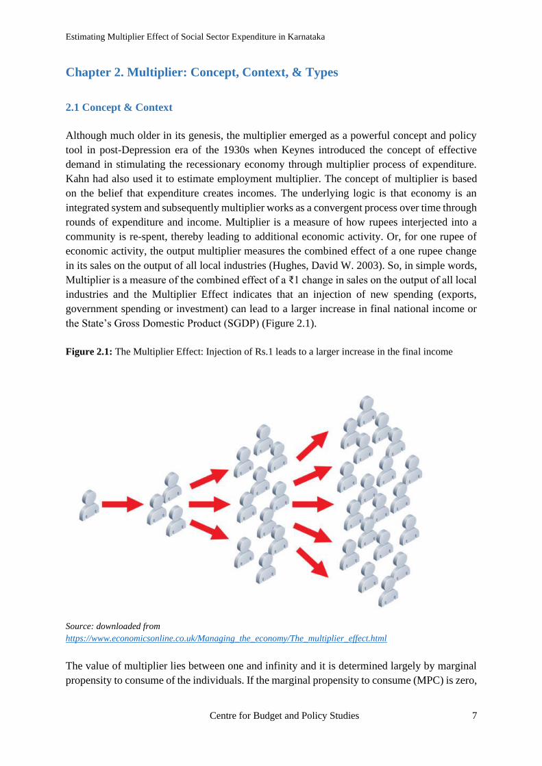
Multiplier is a measure of the combined effect of a ₹1 change in sales on the output of all local
industries and the Multiplier Effect indicates that an injection of new spending (exports,
government spending or investment) can lead to a larger increase in final national income or
the State’s Gross Domestic Product (SGDP) (Figure 2.1).
Figure 2.1: The Multiplier Effect: Injection of Rs.1 leads to a larger increase in the final income
Source: downloaded from
https://www.economicsonline.co.uk/Managing_the_economy/The_multiplier_effect.html
The value of multiplier lies between one and infinity and it is determined largely by marginal
propensity to consume of the individuals. If the marginal propensity to consume (MPC) is zero,
Estimating Multiplier Effect of Social Sector Expenditure in Karnataka
Centre for Budget and Policy Studies 8
the multiplier is one whereas the multiplier is infinity if the MPC is one. The psychological law
of consumption proposed by Keynes says that as income increases, consumption levels increase
up to certain level, but the consumption levels remain constant after a certain rise in income
threshold. From policy planning perspective, it becomes important to understand the MPC and
when it is likely to become constant, as that is the time a higher injection of public spending
needs to be stopped. Any additional injection is not going to create any multiplier effect on the
economy. The multiplier effect on the domestic economy is higher if there are no leakages like
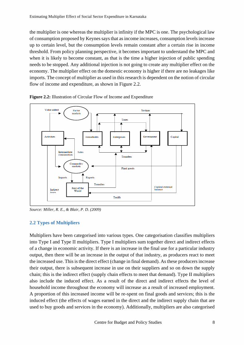
imports. The concept of multiplier as used in this research is dependent on the notion of circular
flow of income and expenditure, as shown in Figure 2.2.
Figure 2.2: Illustration of Circular Flow of Income and Expenditure
Source: Miller, R. E., & Blair, P. D. (2009)
2.2 Types of Multipliers
Multipliers have been categorised into various types. One categorisation classifies multipliers
into Type I and Type II multipliers. Type I multipliers sum together direct and indirect effects
of a change in economic activity. If there is an increase in the final use for a particular industry
output, then there will be an increase in the output of that industry, as producers react to meet
the increased use. This is the direct effect (change in final demand). As these producers increase
their output, there is subsequent increase in use on their suppliers and so on down the supply
chain; this is the indirect effect (supply chain effects to meet that demand). Type II multipliers
also include the induced effect. As a result of the direct and indirect effects the level of
household income throughout the economy will increase as a result of increased employment.
A proportion of this increased income will be re-spent on final goods and services; this is the
induced effect (the effects of wages earned in the direct and the indirect supply chain that are
used to buy goods and services in the economy). Additionally, multipliers are also categorised
Estimating Multiplier Effect of Social Sector Expenditure in Karnataka
Centre for Budget and Policy Studies 9
into output, employment, income and value-added multipliers, depending on how those are
estimated and for what purpose.
2.3 Review of Literature
Empirical Literature generally studies the impact of social sector expenditure on human capital
formation through witnessing improvement in educational enrolment rates and health status of
children in India (Bhakta, 2014) and the positive impact of public investment in education and
health on economic growth (Jung & Thorbecke, 2003). The estimates have varied in different
contexts, e.g., enhanced health expenditures leading to a four per cent increase in output due to
one-year improvement in population life expectancy observed across a panel of countries.
(Bloom et al., 2004) or a one percent increase in total health expenditure leading to a 0.06 –
0.10% increase in per capita GDP growth rate observed in a panel of 19 OCED countries
(Beraldo et al., 2009).
The growth and welfare enhancing effects are found to be most pronounced when they are
financed through a re-composition of public expenditure rather than when they are financed
through increased taxation (Annabi et al., 2011). Further, relationships between maternal and
child health outcomes and economic growth in different countries at different income levels
suggest that the effect of marginal health investments on health outcomes is higher at low levels
of GDP, i.e. in countries where the level of health investments is generally lower (Amiri &
Gerdtham, 2013). Social sectors also involve addressing question of gender inequality and
effect of its improvement on economic growth. Using cross-country regressions, studies have
shown that income and gender inequality jointly impede growth mostly in the initial stages of
development (Hakura et al., 2016, Ahang, 2014, Klasen and Lamanna, 2009). On the other
hand, promoting gender equality, has shown to contribute significantly to economic growth
through accumulation of human capital in the long run (Agénor & Canuto, 2013, Kim, J et al,
2016).
India specific studies assessing the impact of public expenditure on social sectors have found
a large, positive and significant impact of government spending on public goods such as health,
education and basic infrastructure on per capita GDP and poverty. In a panel data analysis of
14 states in India, it was found that a reallocation of expenditures was found to have an average
increase per capita GDP growth rate by 2.7 percentage points and reduce poverty headcount
index by up to 6.6 percentage points (Hong & Ahmed (2009). However, a study using dynamic
CGE modelling (Ganesh Kumar et al., 2017) showed the macro-economic impact of different
types of public expenditure and it showed that social sector expenditure (water, education and
health) does not affect GDP growth.
In this study, we are more interested in understanding the short-term growth enhancing effects
of social sector expenditure using multiplier approach. A good number of studies in this respect
have emanated from Europe. For OECD countries, the domestic aggregate multiplier using
Input Output database was estimated to be 1.61 for the year 1997, which reduced to 1.03 with
imports, and was 1.65 for intermediate sector multipliers (Jones, C. 2007). Similarly, another
Estimating Multiplier Effect of Social Sector Expenditure in Karnataka
Centre for Budget and Policy Studies 10
study for advanced economies using a dynamic stochastic general equilibrium model found
that an unanticipated increase in government investment spending by 1% point increases the
level of output by 0.4% (short term investment multiplier) in the same year whereas four years
later, the medium-term fiscal multiplier turns out to be 1.5%. (ADB, A. A., Furceri, D., & IMF,
P. T. 2016). Fiscal multipliers calculated for 25 EU countries for the years 1995 and 2010 using
Vector Auto Regressive Method to estimate cross-national fixed effects estimated the
multiplier for total government spending to be 1.61 (Reeves, A. et. al 2013).
Furceri & Zdzienicka (2012) conducted an analysis for nine different social policy areas for a
panel of OECD countries from 1980 to 2005 and found that social spending devoted to health
and unemployment benefits are those that have greatest effects. The same results were found
in a Maltese economy using I-O analysis where social work, education, health sector had seen
positive and had large Type II multiplier (Cassar (2015)). It is interesting to see that social
sectors like health had a larger multiplier effect of 4.3 over -9.8 in defence (Reeves et al., 2013)
in a study covering 25 EU countries from 1995 to 2010, both before and during the recession
that began in 2008. The difference in multiplier effects across different types of spending was
explained by varying degrees of absorption of government spending into the domestic
economy. Supply side effects in the local economy is found to be greater than income side
effects implying the need for demand driven economy to have larger multiplier effects
(Domański, B., & Gwosdz, K. 2010). The results are corroborated also by (Micek, G. 2011)
who say that indirect multiplier (Supply side effects) is greater than direct (Income Effect).
However, certain studies also found public expenditure on social sector having very low or no
multiplier effect on growth. Kraay (2012) conducted a study on 29 aid-dependent low-income
countries using two-stage least squares (2SLS) method to calculate contemporaneous spending
multiplier and the estimates show that impact multiplier is mere 0.48. The effect of government
spending in Kenya using Structural VAR for the period 1991-2012 is found to be weak and
this is linked to high debt ratio levels and high marginal propensity to import (Mahrous, 2016).
Nevertheless, in general, the studies undertaken in both developed and developing or low-
income countries have found the multipliers to be positive and high for the social sector
expenditure (Ianchovichina, E., et. al 2012; Furceri & Zdzienicka, 2012; Cassar, 2015; Reeves
et al., 2013; Micek, G., 2011; Domański, B., & Gwosdz, K., 2010).
While IOTT was limited to capturing production structures, Social Accounting Matrix (SAM)
emerged as a tool that helps estimate the distribution effect in addition to understanding
production structure and served as a tool used for policy analysis since the 1960 and 1970s.
Existing literature especially from the developing world with dualistic feature of their
economies, has largely made an attempt to build SAM to understand the effect of increase in
exogenous expenditure either on household incomes or for specific sectoral impacts. SAM built
for Srilanka (Pyatt, G., & Round, J. I., 1979) was one of the early researches on constructing
SAM in developing countries where they found that poverty incidence was high especially
among estate workers and the SAM multiplier analysis showed that this was due to poor
multiplier effect of income injection unless it was injected in tea or rubber sectors. Thorbecke
& Jung (1996) extended an earlier study to understand the sectoral growth and its consequences

Estimating Multiplier Effect of Social Sector Expenditure in Karnataka
Centre for Budget and Policy Studies 11
on poverty reduction and found that agricultural growth had larger effect on poverty reduction
in relation to growth in industrial sector even after accounting for various multiplier effects.
On similar lines, SAM built for Tanzania (Mendez-Parra, M. (2015)) was to gauge sectoral
impact of an increase in final demand on output and different types of labour classified on the
basis of education. The exercise shows that on an average, agriculture sector has the larger
output multiplier effect reflecting stronger final demand components. It was further found that
a shock that increases demand for services tends to have the strongest effect on the output of
the economy but the employment effect is rather modest due to poor backward linkages of
services. Higher employment effects were found in agriculture and fisheries sector due to
strong backward linkages despite lower, though not negligible, output effect. The industrial
sectors have smaller output and employment multiplier effects.
Duality in developing economies persist in both occupational and employment structure that
primarily gave an impetus to build SAM to understand the effect of intervention on labour
market. Defourny, J., & Thorbecke, E. (1984) built SAM for South Korea for the year 1968 to
find the total multipliers for various paths of injections and account destinations. They, in
particular showed the relative importance of paths of the multiplier effects on households
headed by unskilled workers that arise from an injection in the processed foods sector. The
direct effect of this is increase in demand for unskilled labour that would create multiplier effect
of no more than 25% of the total multiplier effect and the remaining is due to linkage effects
or indirect paths.
Further, as part of the OECD country case studies on ‘Adjustment and Equity’ to trace the
impact of government budget reduction in 1980’s on household groups, a study in Indonesia
was conducted through SAM to show that that higher income groups in both rural and urban
areas were largely affected by current expenditure of government while poor income groups
were equally affected by reduction in both exports and current government expenditure
(Keuning, S., & Thorbecke, E., 1992). Similarly, a recent study builds SAM to analyse the
impact on socio-economic activity especially on GDP of the country of an increase in
households’ income in Portugal (Santos, 2018). With household share in the GDP being 60.8%
and their main source of income being compensation to factor services taking the largest share
of 73.8% and current transfers by the government at 23.3%, it was found that origin or source
of increment in household income has different effects with impact on aggregate income being
larger through rise in compensation of employees relative to increase in transfers.
As we are aware that production and distribution are interconnected economic processes,
studies have emphasised on understanding this interdependence. In this context, Powell, M., &
Round, J. I. (2000) constructed SAM for the year 1993 to understand sector specific investment
and its effect on income generation in Ghana. As far as the linkage structure of SAM is
concerned, it was found that an exogenous injection of an extra 100 units of income into the
cocoa sector leads to additional household incomes of 107 in urban areas and 71 in rural areas,
after taking into account the various transfer, spillover and feedback effects. While in terms of
overall income effects, the SAM structure suggests that an exogenous injection of 100 units of
income into the health and education sector would have larger effects on household incomes
Estimating Multiplier Effect of Social Sector Expenditure in Karnataka
Centre for Budget and Policy Studies 12
than an injection into either cocoa or mining (urban 132 and rural 84). Another recent study
was to use SAM to analyse the effects on the Greek economy during the crisis period of 2008,
which established that the recession was derived primarily by the decline in household income
and government spending.
The construction of SAM has not been very common in India. Using India’s IOTT and NSS to
assess income inequality across various households and their respective contribution to
national income, Pal, B. D., & Bandarlage, J. S. (2017) constructed a 78 Sector SAM for India
for the year 2007-08. It claims that ‘Other’ social category which constitutes around 17% of
the total population contribute 13% to the country’s net national income whereas SC
(Scheduled Caste), ST (Scheduled Tribe) and OBC (Other Backward Caste) put together
contribute lesser than their share in the total population in rural areas. Further, the paper claims
that urban counterparts are relatively more productive. Adding to this, the paper claims through
multiplier analysis that growth in paddy would reduce income inequality among SC and ST
households while it is the growth in livestock sector that does the same for OBC households.
Further, Sinha, A et al, (2000) built SAM for India to understand the impact on informal
households’ income of a possible increase in exogenous demand for informal output and
concluded that expansion in informal sector production could generate more informal sector
income. Some studies have attempted to understand the energy sector using SAM approach by
decomposing the sector (Ojha, V et al, 2009; Pradhan, et al, 2014).
Constructing Social Accounting Matrix at a sub-national level is a difficult task with very few
attempts being made in this regard. Ganesh-Kumar & Panda (2014) analysed the impact of
state government spending for consumption and investment, and the consequent spillover
effect of this spending on GDP if done either in the form of central transfer or generating its
own source of revenue by using SAM 2011-12 for India. The analysis showed that states with
high share of manufacturing like Punjab, Kerala, West Bengal or Tamil Nadu contribute high
in terms of national GDP when fiscal transfers are given to these developed states while fiscal
transfers have relatively small spill over effects if given to states like Goa, Odisha, Madhya
Pradesh and Chhattisgarh. By dividing India into four regions namely poor, middle income,
rich and special category states, SAM was constructed for the year 2003-04 separately for these
regions as spatial dimension plays a role (Pradhan, B. K, et al, (2006)). However, for the first
time, a state-level regional SAM was constructed for the state of Andhra Pradesh for the year
2007-08 though largely using India’s coefficients (Saluja, M. R. (2014)).
Based on the review of literature, that establishes the usefulness of IOTT and SAM as tools for
the measurement of multipliers as a policy choice tool, we chose these two tools to estimate
the multiplier effect of social sector expenditure in Karnataka. Although these tools have been
largely used to understand the industry specific multipliers, we have used these to understand
the structure of the Karnataka’s economy and calculate multiplier effect of social sector
expenditure in particular. In the process, this became one of the first study to use variety of
data sources to overcome the challenge of lack of adequate data at sub-national level, which
we describe in detail as we go further.

Estimating Multiplier Effect of Social Sector Expenditure in Karnataka
Centre for Budget and Policy Studies 13
2.4 Methods used to estimate Multiplier
Supply based growth theories that rests on the belief that the free enterprise economy is self-
regulating, demand based growth theories on the other hand believe that growth process is path
dependent and cumulative. Past affects the present and the future and therefore history is
imperative in the economy’s growth process. They view the growth process as non-linear, and
therefore historical. This implies that demand-based growth theories call for active government
intervention in stimulating growth that could be far away from natural rate of growth. In these
theories, demand deficiency is a structural problem that can be corrected only with government
intervention through policies that increase aggregate demand either through increase in
consumption expenditure or autonomous investment expenditure. It therefore addresses the
question of both availability and more importantly affordability. These theories depend on a
frame that understands economy as an integrated system and production as a social activity.
There are various methods and tools to estimate multiplier and broadly these can be classified
into conventional approaches (neoclassical) and alternative approaches. The tools under
conventional (neoclassical) approaches include Vector Auto-Regressive methods, Computable
General Equilibrium method and Dynamic Stochastic General Equilibrium Method. These
tools under conventional Approaches believe in supply side theories where investment is
dependent variable. Alternative approaches on the other hand include Input-Output Model
(IOM) and Social Accounting Matrix (SAM) which believes in integrated economic system
and investment as an autonomous variable. We have used alternative methods following the
demand side approach.
2.4.1 Input-Output Models
Input-Output Table is an accounting framework generally constructed for a specific geographic
region for a specified period, say, a year, and is concerned with the activity of a group of
industries that both produce goods (outputs/producer) and consume goods from itself or other
industries (inputs/consumers) in the process of producing each industry’s own output. It shows
the flows of goods and services from each branch of the economy to different branches of the
economy. The basic information from I-O is presented in the inter-industry transactions table.
The rows of the table describe the distribution of a producer’s output throughout the economy
while the columns describe the composition of inputs required by a particular industry to
produce its output. The additional columns constitute the components of Final Demand that
records the sales of each sector to final markets either for personal use or use by government.

Estimating Multiplier Effect of Social Sector Expenditure in Karnataka
Centre for Budget and Policy Studies 14
Figure 2.3: Input - Output Table Representation
Source: Miller, R. E., & Blair, P. D. (2009)
In a nutshell, it presents the intermediate inputs in the production of goods and services by
various sectors as well as towards the final consumption. I-O clearly captures the circular flow
and the interdependence between sectors by providing detailed disaggregated quantitative
description of the structural characteristics of all component parts of a given economic system.
Using I-O Table, one can understand the structural characteristics of an economy and it helps
identify those key sectors that stimulate growth which would induce specific investments
especially when there is slowdown and unequal growth. One of the main limitations, however,
is that represents a stationary system characterised by constant technical coefficients.
Estimating Multiplier Effect of Social Sector Expenditure in Karnataka
Centre for Budget and Policy Studies 15
Construction of I-O Tables that are comprehensive and consistent helps us understand how
growth has changed the ratio of intermediate use in the total gross output as against the ratio of
factor inputs used in the total gross output. It helps us see the linkage structures if we do an
intertemporal comparison of I-O Table. The tool helps in forecasting of supply and demand in
the economy for a target year.
2.4.2 Social Accounting Matrix
A useful extension of I-O matrix is Social Accounting Matrix, a tool that explicitly puts
emphasis on distribution and its interaction with production as against I-O which largely
focuses on production structure. Income Distribution is a key in a capitalist economic
organisation because demand matters for the long run growth of the economy. Capitalist
economies are monetary production economies where monetary circuit establishes both
Backward and Forward Linkages
It is important to understand the notion of backward and forward linkages as economy is an
integrated system representing in the context of a circular flow of income and expenditure.
Hirschman defines the backward linkage effect as a "non-primary" activity, i.e., an activity that
employs significant amounts of intermediate inputs from other activities, should be expected
to induce attempts to supply these inputs through expanding domestic production. A forward
linkage effect is defined as an activity that is "non-final," i.e., an activity that does not cater
exclusively to final demand, should be expected to induce attempts to utilise its outputs as
inputs in some new activities (Bhattacharya, T., & Rajeev, M. (2014).
The linkage effects help us identify the core or key sectors of an economy that have the capacity
to stimulate the growth of other sectors either through providing their own output to other
sectors (forward linkage), or through taking inputs from other sectors (backward linkage). In
simple terms, backward linkage expresses how a sector depends on others for input supplies
while forward linkage identifies how a sector distributes its output to the remaining economy.
The intensity of linkages reflects the potential capacity of each sector to stimulate other sectors
and economy in general.
The idea of backward and forward linkages arises from the fact that economy is an integrated
system where all sectors are interconnected implying existence of vertical integration set up.
The extent of sectoral integration reflects the significance of the sector in the economy. Sectoral
linkages describe the sector’s direct and indirect association through its direct and indirect
purchases and sales of direct and intermediate inputs with the rest of the sectors in the economy.
A forward linkage is created when investment in a sector creates investment in subsequent
stages of production. Forward production linkages refer to the part of the non-farm sector that
uses agricultural output as input in its production, for instance, silk worm in the silk production.
A backward linkage is created when an investment creates or facilitates those facilities that
require that investment. Backward production linkages refer to the linkages from the farm to
the part of the non-farm sector that provides inputs for agricultural production for instance
demand increases for say, fertilisers or tractors or agrochemicals.
We can say backward linkages are directed towards suppliers and forward linkages are directed
towards consumers.

Estimating Multiplier Effect of Social Sector Expenditure in Karnataka
Centre for Budget and Policy Studies 16
circular flow of income between economic sectors and also links economic units like
households, firms, governments to each other over time. SAM tends to capture these links and
interactions. SAM was built as an improvement to I-O to capture better information on
distribution and final demand. The income distributional conflicts and effects of policies in a
developing economy is important as it captures the inequalities through the linkage between
value added and final demand.
SAM is a matrix representation of national income accounts (Figure 2.4) and this framework
serves to satisfy two basic rules (Pyatt & Round, 1977):
1. For every row there is a corresponding column, and the system is complete only if the
corresponding row and column totals are identical; and
2. Every entry is a receipt when read in its row context, and expenditure in its column context.
Purpose of Social Accounting Matrix
SAM, a summary table highlighting the interlinkages and the circular flow of payments and
receipts among the different components of the system such as goods, activities, factors, and
institutions, fulfils following purposes:
• It helps organise the information on the social and economic structure of a country
for a given period.
• It provides a synoptic view of the flows of receipts and payments in an economic
system;
• It represents together production, income generation, consumption, investment and
external transaction.
• It forms a statistical basis for building models of the economic system, with a view
to use this to simulate the socio-economic impact of policies.
• SAM is social as it captures the social background of Households unlike IO which
accounts only economic transactions/functional activities.
• SAM as a technique is flexible. It has a basic accounting structure but gives scope
for disaggregation.
• SAM, vouches to understand, ‘Growth with Distribution’ and
SAM is not limited to understand the real economy transactions. It can be extended to
include the interaction between real and financial economy.
Estimating Multiplier Effect of Social Sector Expenditure in Karnataka
Centre for Budget and Policy Studies 17
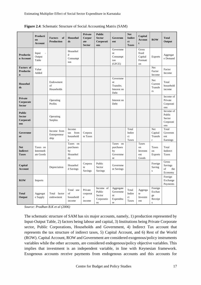
Figure 2.4: Schematic Structure of Social Accounting Matrix (SAM)
Producti
on
Account
Factors of
Production
Househol
ds
Private
Corpor
ate
Sector
Public
Sector
Corporati
ons
Governm
ent
Net
Indire
ct
Taxes
Capital
Accoun
t
ROW Total
Output
Productio
n Account
Input -
Output
Table
Househol
d
Consumpt
ion
Governme
nt
Consumpt
ion
(GFCE)
Gross
fixed
Capital
Formati
on
Exports Aggregat
e Demand
Factors of
Productio
n
Value
Added
Net
Factor
Income
Factor
Income
Househol
ds
Endowment
of
Households
Governme
nt
Transfer,
Interest on
Debt
Net
Current
Transfe
rs
Total
household
income
Private
Corporate
Sector
Operating
Profits
Interest on
Debt
Income of
Private
Corporati
ons
Public
Sector
Corporati
ons
Operating
Surplus
Income of
Public
Sector
Corporati
ons
Governme
nt
Income from
Entrepreneur
ship
Income
tax from
household
s
Corpora
te Taxes
Total
Indire
ct
Taxes
Net
Capital
Transfe
r
Total
Governm
ent
Earnings
Net
Indirect
Taxes
Taxes on
Intermedi
ate Goods
Taxes on
purchases
by
Househol
ds
Taxes on
purchases
by
Governme
nt
Taxes
on
Investm
ent
Goods
Taxes
on
Exports
Total
Indirect
Taxes
Capital
Account Depreciation
Househol
d Savings
Corpora
te
Savings
Public
Sector
Savings
Governme
nt Savings
Foreign
Saving
s
Gross
Savings
of the
Economy
ROW Imports
Foreign
Exchange
Payments
Total
Output
Aggregat
e Supply
Total factor
endowment
Total use
of
household
income
Private
corporat
e
income
Income of
Public
Sector
Corporatio
ns
Aggregate
Governme
nt
Expenditu
re
Total
Indire
ct
Taxes
Aggrega
te
Investm
ent
Foreign
Exchan
ge
Receipt
s
Source: Pradhan B.K et al (2006)
The schematic structure of SAM has six major accounts, namely, 1) production represented by
Input-Output Table, 2) factors being labour and capital, 3) Institutions being Private Corporate
sector, Public Corporations, Households and Government, 4) Indirect Tax account that
represents the tax structure of indirect taxes, 5) Capital Account, and 6) Rest of the World
(ROW). Capital Account, ROW and Government are considered exogenous/policy instruments
variables while the other accounts, are considered endogenous/policy objective variables. This
implies that investment is an independent variable, in line with Keynesian framework.
Exogenous accounts receive payments from endogenous accounts and this accounts for
Estimating Multiplier Effect of Social Sector Expenditure in Karnataka
Centre for Budget and Policy Studies 18
leakages in the economic system as these do not contribute to the multiplicative process and
skip the expenditure stream. So, the matrix enables the effects of exogenous expenditure to be
transmitted to the economic system through multiplier impact that follow an iterative circuit of
production, use and distribution of income. Annexure 1 discusses these in detail.
Estimating Multiplier Effect of Social Sector Expenditure in Karnataka
Centre for Budget and Policy Studies 19
Chapter 3. Construction of IOTT and SAM for Karnataka 2013-14
3.1 Background
I-O Table as a tool made its inroads in the post-independence era of India and played a key role
in the planning process of India. The first I-O Table was prepared in India by the Central
Statistical Office (CSO) in the year 1968-69 and subsequently it was constructed for 1973-74,
1978-79, 1983-84, 1989-90, 1993-94, 1998-99, 2003-04 and lastly for the year 2007-08 which
was the last official I-O table available in the public domain. However, CSO has been
publishing Supply and Use Tables (SUT) with the latest one being for the year 2015-16. SUT
as a key feature of national accounts provides data that links output of industries as products,
and intermediate and final uses of various products. It helps compile Gross Domestic Product
(GDP) at current prices and provides the ideal concept for balancing supply and demand (CSO,
2016).
The construction of the I-O Table at the sub-national / regional level is significant as it provides
a comprehensive, detailed and consistent framework of the structure of the production system
within the boundaries of that state. Considering that the Indian states are very different from
each other in terms of its history, economic size and composition and structures of production
Supply and Use Table (SUT) and I-O Table
SUT provides a base for the construction of I-O table. I-O model provides a link between
supply and demand levels for different sectors. It is a theoretical scheme where the final
demand components are exogenously determined.
The supply use equation for any given product in an economy can be mathematically
expressed as:
Output + Imports = Intermediate consumption + Final consumption + Gross
capital formation (including changes in stocks and valuables) + Exports
or also can be re-written as:
Output – Intermediate consumption + Taxes on products – Subsidies on products
= Final consumption (government and private) + Gross capital formation (fixed,
changes in stocks and valuables) + Exports – Imports
I-O Table is based on the following assumptions:
a. Each sector produces homogeneous good and there is no scope for substitutability
between the outputs of different sectors.
b. The production function is assumed to be of Leontief form where fixed
proportions of inputs are used by the sector to produce a particular level of output
and that implies inputs varies in direct proportion to change in output.
The other condition is called as Hawkins Simons condition that ensure viability in the
economic system. This means, there is surplus in the economy, i.e. amount of output used
as input should be less than the total output.

Estimating Multiplier Effect of Social Sector Expenditure in Karnataka
Centre for Budget and Policy Studies 20
that also tend to change over time. Hence, it can be useful for policy makers to adopt or re-
structure policies based on the impact it might have on the production structure. This is
significant especially when we follow a federal system of functioning. However, constructing
the I-O Table at the regional level is relatively more difficult as many of the parameters which
form components of the I-O table are not measured at the sub-national level at present and there
is very little work being done in this area of research.
We constructed I-O Table and SAM for Karnataka for the year 2013-14. The choice of the year
was because the updated Indian IOTT constructed for India is for the year 2013-14 (Saluja &
Singh 2017). While we made every effort to use state specific data-sources for arriving at sector
specific coefficients by using data-sources that have not been used earlier, we were forced to
use national level coefficients in certain cases for lack of any credible alternative, and thereby
The Input-Output table: A simple representation
To understand what the values in the matrix mean, the values X11 to X33 represents the
intermediate consumption in each destination sector, of the input coming from the originating
sector. For example, X23 represents the value of intermediate consumption in sector 3
(destination sector) of the inputs coming from sector 2 (originating sector). T1 to T3 gives the
summation of all the inputs coming from that particular originating sector.
Intermediate Use Matrix Final Demand Components (GVA)
Total
Outpu
t
(GVO
)
Consuming
(Destinatio
n)Sector /
Producing
(Originatin
g) Sector
Sector 1 Sector 2 Sector 3 IUSE PFCE GFCE GFCF Export
s
Impo
rts
Tot.
Final
Use
(GVA)
Sector 1 X11 X12 X13 T1 P1
Sector 2 X21 X22 X23 T2 P2
Sector 3 X31 X32 X33 T3 P3
Total Input X1 X2 X3
Gross
Value
Added
(GVA)
Net Taxes
Total
Output
In order to calculate the final demand components, which add up to the total final use or the
Gross Value Added (GVA), we need to calculate each of the individual components that
include PFCE, GFCE, GFCF, Exports and Imports.
Total Input + GVA + Net Indirect Taxes = GVO = Intermediate Consumption + GVA
or
Total Use (Demand) = Total Supply

Estimating Multiplier Effect of Social Sector Expenditure in Karnataka
Centre for Budget and Policy Studies 21
assuming that these are the same for state and national levels in those specific instances.
Although this may be considered one limitation of this study, so far, all other state-level I-O
Tables have shown far more dependence on national coefficients, and in that respect, ours is
far more state-centric in its rigour and specificity2. In this section we present the
methodological steps along with data sources and process of computation for the various
components of I-O Table and SAM in brief while the details have been presented in Annexures
2,3,4,5.
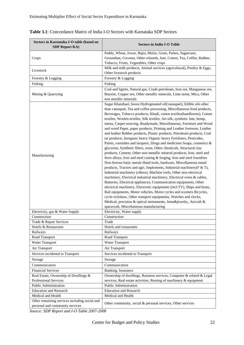
3.2 Mapping of the Karnataka SDP sectors against India’s I-O Table
The I-O Table constructed for India in 2013-14 by NCAER is a detailed table and contains
130*130 sectors (commodity*commodity table). We mapped these against 23 sectors primarily
based on the sector classification available in the State Domestic Product (SDP) Report of
Karnataka for 2016-17 in order to construct 23*23 sector*sector table (Table 3.1). Further, for,
aligning with the objectives of our study, we have disaggregated the category ‘Other Services’
to identify Education & Research and Medical & Health as separate categories. This would
help us obtain the multiplier for the Education and Health sectors separately.
2 The exercise can be considered first of its kind in a way because of the rigour with which it has been undertaken
to a certain extent. The process of compilation included meetings with state officials of the Economics and
Statistics department to understand the data collection processes, personally gathering annual reports of Public
Sector Undertakings under the purview of the Karnataka government. It also involved seeking information which
is supposed to be available in public domain but is not so making us rely on the Right to Information Act (RTI).
The exercise is also significant in a sense as for the first time we have been able to calculate the final demand
components and been able to estimate the shares of each in the total Gross State Domestic Product (GSDP) of
Karnataka
Estimating Multiplier Effect of Social Sector Expenditure in Karnataka
Centre for Budget and Policy Studies 22
Table 3.1: Concordance Matrix of India I-O Sectors with Karnataka SDP Sectors
Sectors in Karnataka I-O table (based on
SDP Report KA) Sectors in India I-O Table
Crops
Paddy, Wheat, Jowar, Bajra, Maize, Gram, Pulses, Sugarcane,
Groundnut, Coconut, Other oilseeds, Jute, Cotton, Tea, Coffee, Rubber,
Tobacco, Fruits, Vegetables, Other crops
Livestock Milk and milk products, Animal services (agricultural), Poultry & Eggs,
Other livestock products
Forestry & Logging Forestry & Logging
Fishing Fishing
Mining & Quarrying
Coal and lignite, Natural gas, Crude petroleum, Iron ore, Manganese ore,
Bauxite, Copper ore, Other metallic minerals, Lime stone, Mica, Other
non metallic minerals
Manufacturing
Sugar Khandsari, boora Hydrogenated oil(vanaspati), Edible oils other
than vanaspati, Tea and coffee processing, Miscellaneous food products,
Beverages, Tobacco products, Khadi, cotton textiles(handlooms), Cotton
textiles, Woolen textiles, Silk textiles, Art silk, synthetic Jute, hemp,
mesta, Carpet weaving, Readymade, Miscellaneous, Furniture and Wood
and wood Paper, paper products, Printing and Leather footwear, Leather
and leather Rubber products, Plastic products, Petroleum products, Coal
tar products, Inorganic heavy Organic heavy Fertilisers, Pesticides,
Paints, varnishes and lacquers, Drugs and medicines Soaps, cosmetics &
glycerine, Synthetic fibers, resin, Other chemicals, Structural clay
products, Cement, Other non-metallic mineral products, Iron, steel and
ferro alloys, Iron and steel casting & forging, Iron and steel foundries
Non-ferrous basic metals Hand tools, hardware, Miscellaneous metal
products, Tractors and agri. Implements, Industrial machinery(F & T),
Industrial machinery (others), Machine tools, Other non-electrical
machinery, Electrical industrial machinery, Electrical wires & cables,
Batteries, Electrical appliances, Communication equipments, Other
electrical machinery, Electronic equipments (incl.TV), Ships and boats,
Rail equipments, Motor vehicles, Motor cycles and scooters Bicycles,
cycle-rickshaw, Other transport equipments, Watches and clocks,
Medical, precision & optical instruments, Jems&jewelry, Aircraft &
spacecraft, Miscellaneous manufacturing
Electricity, gas & Water Supply Electricity, Water supply
Construction Construction
Trade & Repair Services Trade
Hotels & Restaurants Hotels and restaurants
Railways Railways
Road Transport Road Transport
Water Transport Water Transport
Air Transport Air Transport
Services incidental to Transport Services incidental to Transport
Storage Storage
Communication Communication
Financial Services Banking, Insurance
Real Estate, Ownership of Dwellings &
Professional Services
Ownership of dwellings, Business services, Computer & related & Legal
services, Real estate activities, Renting of machinery & equipment
Public Administration Public Administration
Education and Research Education and Research
Medical and Health Medical and Health
Other remaining services including social and
personal and community services Other community, social & personal services, Other services
Source: SDP Report and I-O Table 2007-2008
Estimating Multiplier Effect of Social Sector Expenditure in Karnataka
Centre for Budget and Policy Studies 23
3.3 Process towards the construction of IOTT and SAM for Karnataka 2013-14
The Input-Output table can be divided into two major parts, the intermediate use (consumption)
matrix (IC matrix) and the final demand components. Computation of both the parts involves
extensive analyses and clubbing of data from various sources.
3.3.1 Gross Value of Output (GVO)
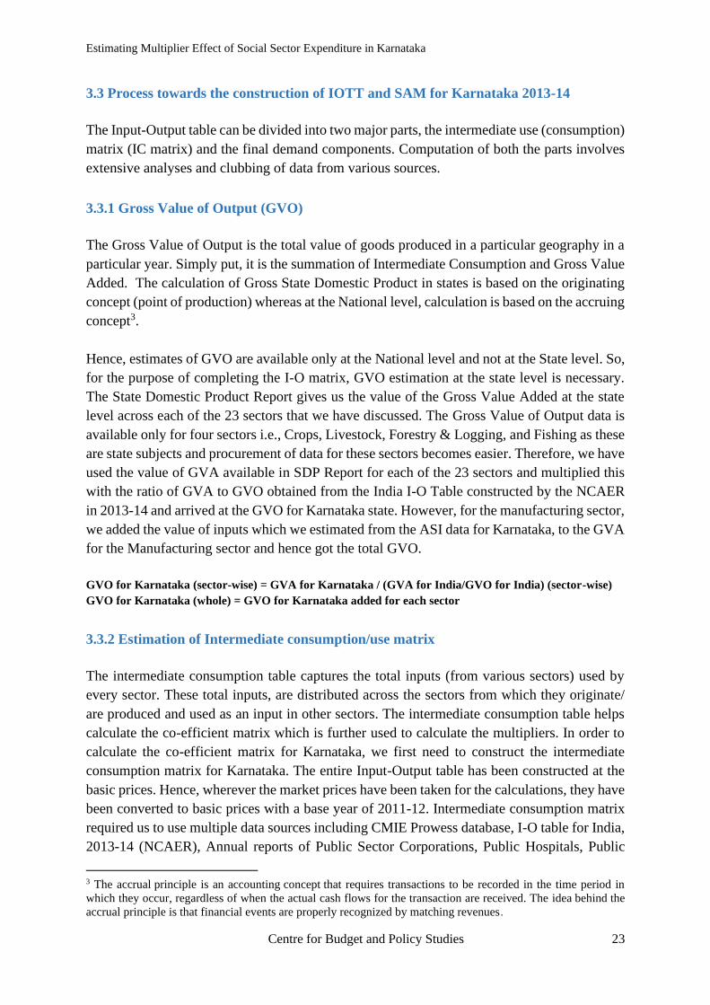
The Gross Value of Output is the total value of goods produced in a particular geography in a
particular year. Simply put, it is the summation of Intermediate Consumption and Gross Value
Added. The calculation of Gross State Domestic Product in states is based on the originating
concept (point of production) whereas at the National level, calculation is based on the accruing
concept3.
Hence, estimates of GVO are available only at the National level and not at the State level. So,
for the purpose of completing the I-O matrix, GVO estimation at the state level is necessary.
The State Domestic Product Report gives us the value of the Gross Value Added at the state
level across each of the 23 sectors that we have discussed. The Gross Value of Output data is
available only for four sectors i.e., Crops, Livestock, Forestry & Logging, and Fishing as these
are state subjects and procurement of data for these sectors becomes easier. Therefore, we have
used the value of GVA available in SDP Report for each of the 23 sectors and multiplied this
with the ratio of GVA to GVO obtained from the India I-O Table constructed by the NCAER
in 2013-14 and arrived at the GVO for Karnataka state. However, for the manufacturing sector,
we added the value of inputs which we estimated from the ASI data for Karnataka, to the GVA
for the Manufacturing sector and hence got the total GVO.
GVO for Karnataka (sector-wise) = GVA for Karnataka / (GVA for India/GVO for India) (sector-wise)
GVO for Karnataka (whole) = GVO for Karnataka added for each sector
3.3.2 Estimation of Intermediate consumption/use matrix
The intermediate consumption table captures the total inputs (from various sectors) used by
every sector. These total inputs, are distributed across the sectors from which they originate/
are produced and used as an input in other sectors. The intermediate consumption table helps
calculate the co-efficient matrix which is further used to calculate the multipliers. In order to
calculate the co-efficient matrix for Karnataka, we first need to construct the intermediate
consumption matrix for Karnataka. The entire Input-Output table has been constructed at the
basic prices. Hence, wherever the market prices have been taken for the calculations, they have
been converted to basic prices with a base year of 2011-12. Intermediate consumption matrix
required us to use multiple data sources including CMIE Prowess database, I-O table for India,
2013-14 (NCAER), Annual reports of Public Sector Corporations, Public Hospitals, Public
3 The accrual principle is an accounting concept that requires transactions to be recorded in the time period in
which they occur, regardless of when the actual cash flows for the transaction are received. The idea behind the
accrual principle is that financial events are properly recognized by matching revenues.
Estimating Multiplier Effect of Social Sector Expenditure in Karnataka
Centre for Budget and Policy Studies 24
Universities, SSA, RMSA, Commissionerate of Public Instruction, Medical Education, KGBV
Accounts, Directorate of Economics and Statistics (Crops Inputs), Annual Survey of Industries.
Annexure 2 discusses the step-by-step details of constructing the input structure along with the
assumptions used and details of how these data sources were used for different sectors.
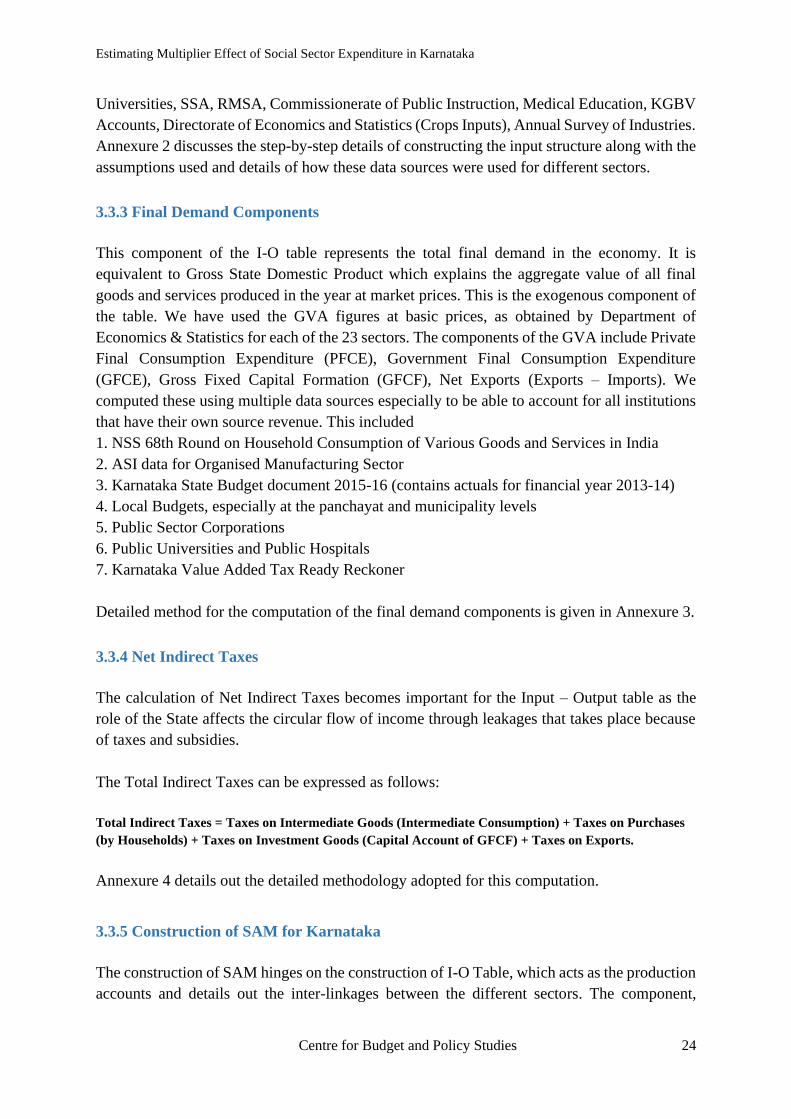
3.3.3 Final Demand Components
This component of the I-O table represents the total final demand in the economy. It is
equivalent to Gross State Domestic Product which explains the aggregate value of all final
goods and services produced in the year at market prices. This is the exogenous component of
the table. We have used the GVA figures at basic prices, as obtained by Department of
Economics & Statistics for each of the 23 sectors. The components of the GVA include Private
Final Consumption Expenditure (PFCE), Government Final Consumption Expenditure
(GFCE), Gross Fixed Capital Formation (GFCF), Net Exports (Exports – Imports). We
computed these using multiple data sources especially to be able to account for all institutions
that have their own source revenue. This included
1. NSS 68th Round on Household Consumption of Various Goods and Services in India
2. ASI data for Organised Manufacturing Sector
3. Karnataka State Budget document 2015-16 (contains actuals for financial year 2013-14)
4. Local Budgets, especially at the panchayat and municipality levels
5. Public Sector Corporations
6. Public Universities and Public Hospitals
7. Karnataka Value Added Tax Ready Reckoner
Detailed method for the computation of the final demand components is given in Annexure 3.
3.3.4 Net Indirect Taxes
The calculation of Net Indirect Taxes becomes important for the Input – Output table as the
role of the State affects the circular flow of income through leakages that takes place because
of taxes and subsidies.
The Total Indirect Taxes can be expressed as follows:
Total Indirect Taxes = Taxes on Intermediate Goods (Intermediate Consumption) + Taxes on Purchases
(by Households) + Taxes on Investment Goods (Capital Account of GFCF) + Taxes on Exports.
Annexure 4 details out the detailed methodology adopted for this computation.
3.3.5 Construction of SAM for Karnataka
The construction of SAM hinges on the construction of I-O Table, which acts as the production
accounts and details out the inter-linkages between the different sectors. The component,

Estimating Multiplier Effect of Social Sector Expenditure in Karnataka
Centre for Budget and Policy Studies 25
factors include the wage and non-wage component of the GVA and the net factor income from
ROW in the row totals and the total factor endowments in the columns include the endowment
of households, operating profits of private corporations, operating surplus for the public sector
corporations, the income from entrepreneurship earned by the Governments and the
depreciation on the capital account.
Different methods and sources have been used to capture the wage and non-wage component
of the GVA of each sector including agriculture, manufacturing, others that main include
services, education, research, medical and health. Annexure 5 describes the details regarding
how these were classified and computed. The annexure also describes how we estimated the
endowment of households, the operating profits for private sector in the state, operating surplus
of public undertakings, income from entrepreneurship, depreciation on capital account, net
factor income and finally the total factor endowments and the total factor income.
Using the sources mentioned above and the methodology described in the annexures, we
constructed the I-O table and SAM for Karnataka for 2013-14. Based on existing empirical
work, we can state that the share of the final demand components has neither been
overestimated nor underestimated. The I-O Table and SAM computed for Karnataka for the
year 2013-14 are attached as Annexure 9 and Annexure 104.
4 In Excel sheets

Estimating Multiplier Effect of Social Sector Expenditure in Karnataka
Centre for Budget and Policy Studies 26
Chapter 4. Analysis and Discussions
In this chapter, we present the key results of some of the computations and analyse the
multiplier values and their implications for Karnataka’s public policy choices. It is not only the
multiplier values but also other computations undertaken to arrive at multiplier values that
provide us with key pointers for policy choices.
4.1 Components of Aggregate Demand
Aggregate Demand components help us know the structure and discern the drivers of the
growth process. Constructing SAM and IOTT helped us bifurcate the total GVA into its
demand components where the share of the PFCE is 50% while GFCE is 10%, GFCF is 39%
and Net Exports is 1% of GSDP (Figure 4.1).
Figure 4.1: Share of final demand components in GSDP
Source: Authors’ calculations
Intermediate consumption as a proportion of GVO forms 52% of the total GVO. This shows
that consumption expenditure drives the growth process in the state of Karnataka. It further
implies that domestic demand as against external demand plays a pivotal role in growth
meaning that the state’s economy is not dependent on exports in any major manner. Table 4.1
further shows that share of the total inputs in the total Gross Output is around 52% while GVA
as share of the GVO amounts to 47.6%.
50%
10%
39%
1%
PFCE GFCE GFCF X-M

Estimating Multiplier Effect of Social Sector Expenditure in Karnataka
Centre for Budget and Policy Studies 27
Table 4.1: Share of Aggregate Demand Components in Final GSDP (2013-14)
Share of Aggregate Demand Components in Total GSDP and GVO (Rs. Lakhs)
Values in Rs. Lakhs as % GVA As %GVO
PFCE 37277473 50% 24%
GFCE 7154303 10% 5%
GFCF 28922238 39% 18%
X-M 749099 1% 0%
IC 84346330
53%
GVA 74103113
47%
GVO 158449443
Source: Authors’ calculations
4.2 Decomposition of Gross Value Added
The net social product after replenishing for the inputs from the total outputs gives us the
estimate for value addition. Net income or Gross Value Added can also be expressed as a sum
of wage and non-wage income, which is one of the three ways to look at GVA apart from the
lens of production and expenditure. GVA from Income method includes the sum of all factor
incomes earned by all factors across all sectors of the economy. Wage Income involves
remuneration to labour services while Non-wage Income includes income that accrues to
capitalists and landlords in the form of profits, rent and interest. The classification of income
expressed as wage and non-wage income instead of wage and capital income is to account for
the self-employment that exists in the state and therefore to capture the mixed income that they
accrue.
At a state level, one can observe that the wage income component comprises of 41% of the
total GVA while non-wage share is 59%. Further, the wage and non-wage share of GVA across
primary, secondary and tertiary sectors shows varied patterns. Agriculture and allied activities
show almost equal shares of wage and non-wage income, while within secondary sector,
Electricity, Gas & Water Supply and Mining & Quarrying show larger shares of non-wage
income due to huge indivisibility of fixed factors that’s a characteristic of the sectors with wage
income less than 30% share in GVA. In addition, as expected construction (65%) is relatively
more labour intensive than manufacturing sector (50%) within secondary sectors. One can
claim that in an aggregate sense, primary and secondary sectors are relatively more labour
intensive than tertiary sector, also indicating towards the employment potential of these sectors.
However, the components of the tertiary sector show diverse patterns. The wage shares are the
highest for the Education & Research and Medical & Health, and Public Administration,
among the 23 considered sectors. The wage income share in the total GVA of Education and
Health is 89% and 75% respectively while non-wage share is merely 11% and 25%
respectively, implying the high employment potential of these social sectors (Figure 4.2).
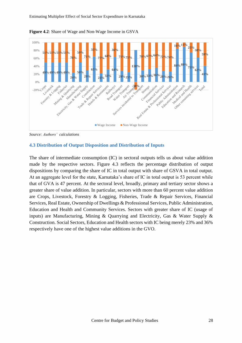
Estimating Multiplier Effect of Social Sector Expenditure in Karnataka
Centre for Budget and Policy Studies 28
Figure 4.2: Share of Wage and Non-Wage Income in GSVA
Source: Authors’ calculations
4.3 Distribution of Output Disposition and Distribution of Inputs
The share of intermediate consumption (IC) in sectoral outputs tells us about value addition
made by the respective sectors. Figure 4.3 reflects the percentage distribution of output
dispositions by comparing the share of IC in total output with share of GSVA in total output.
At an aggregate level for the state, Karnataka’s share of IC in total output is 53 percent while
that of GVA is 47 percent. At the sectoral level, broadly, primary and tertiary sector shows a
greater share of value addition. In particular, sectors with more than 60 percent value addition
are Crops, Livestock, Forestry & Logging, Fisheries, Trade & Repair Services, Financial
Services, Real Estate, Ownership of Dwellings & Professional Services, Public Administration,
Education and Health and Community Services. Sectors with greater share of IC (usage of
inputs) are Manufacturing, Mining & Quarrying and Electricity, Gas & Water Supply &
Construction. Social Sectors, Education and Health sectors with IC being merely 23% and 36%
respectively have one of the highest value additions in the GVO.
49%49%49%49%
24%
50%
29%
65%
23%32%
64%
29%25%
130%
30%33%36%28%26%
84%89%75%
62%
41%
51%51%51%51%
76%
50%
71%
35%
77%68%
36%
71%75%
-30%
70%67%64%72%74%
16%11%25%
38%
59%
-20%
0%
20%
40%
60%
80%
100%
Wage Income Non-Wage Income

Estimating Multiplier Effect of Social Sector Expenditure in Karnataka
Centre for Budget and Policy Studies 29
Figure 4.3: Distribution of Output Disposition
Source: Authors’ calculations
Figure 4.4: Percentage Distribution of Inputs
Source: Authors’ calculations
Figure 4.4 reflects the distribution of inputs into material inputs/commodities and services in
the total inputs used in the production process. This shows that several of the 23 sectors are
material inputs driven while this is least true for the financial services sector followed by
Storage sector. The share of commodities in total inputs is 81% in Education and while it is
only 30% for Health. This analysis is of significance as it tells us that despite the fact that
service sector growth has driven the growth at an aggregate level in Karnataka, the intensity of
services as inputs is relatively less. A temporal analysis, however, may give us a better picture
about the services sector and its growth in other sectors therefore explaining inter sectoral
linkages much better.
16%31%
18% 15%
43%
77% 75%65%
29%47%
36%56% 64%
88%
57% 52% 59%
24% 29% 25%23%36%
47%
83%69%91%
85%
57%
23% 25%35%
71%53%
64%44% 36%
12%
43% 48% 41%
76% 71% 75%77%64%
53%
-10%
10%
30%
50%
70%
90%
110%
Share of Intermediate Consumption in Total GVO Share of Factor Incomes/GVA in Total GVO
65%91%
77% 85% 84% 90% 93% 84% 91%
56%83%79%
68%91%
48%24%
52%
3%
47%67%
81%
30%
74%
35%
31%
23% 14% 16% 10% 7% 16% 9%
44%17%21%
31%9%
53%75%
48%
97%
53%33%
19%
70%
24%
-10%
10%
30%
50%
70%
90%
110%
Share of Commodities/material inputs in total IC Share of Services in Total IC
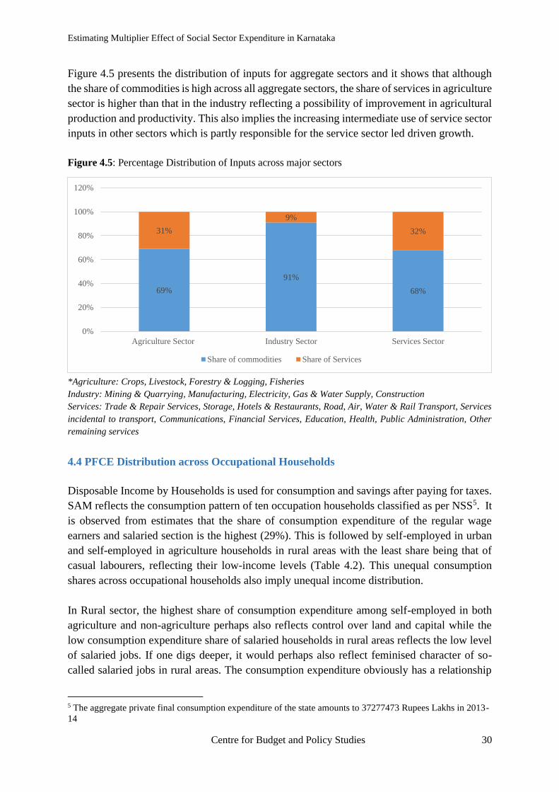
Estimating Multiplier Effect of Social Sector Expenditure in Karnataka
Centre for Budget and Policy Studies 30
Figure 4.5 presents the distribution of inputs for aggregate sectors and it shows that although
the share of commodities is high across all aggregate sectors, the share of services in agriculture
sector is higher than that in the industry reflecting a possibility of improvement in agricultural
production and productivity. This also implies the increasing intermediate use of service sector
inputs in other sectors which is partly responsible for the service sector led driven growth.
Figure 4.5: Percentage Distribution of Inputs across major sectors
*Agriculture: Crops, Livestock, Forestry & Logging, Fisheries
Industry: Mining & Quarrying, Manufacturing, Electricity, Gas & Water Supply, Construction
Services: Trade & Repair Services, Storage, Hotels & Restaurants, Road, Air, Water & Rail Transport, Services
incidental to transport, Communications, Financial Services, Education, Health, Public Administration, Other
remaining services
4.4 PFCE Distribution across Occupational Households
Disposable Income by Households is used for consumption and savings after paying for taxes.
SAM reflects the consumption pattern of ten occupation households classified as per NSS5. It
is observed from estimates that the share of consumption expenditure of the regular wage
earners and salaried section is the highest (29%). This is followed by self-employed in urban
and self-employed in agriculture households in rural areas with the least share being that of
casual labourers, reflecting their low-income levels (Table 4.2). This unequal consumption
shares across occupational households also imply unequal income distribution.
In Rural sector, the highest share of consumption expenditure among self-employed in both
agriculture and non-agriculture perhaps also reflects control over land and capital while the
low consumption expenditure share of salaried households in rural areas reflects the low level
of salaried jobs. If one digs deeper, it would perhaps also reflect feminised character of so-
called salaried jobs in rural areas. The consumption expenditure obviously has a relationship
5 The aggregate private final consumption expenditure of the state amounts to 37277473 Rupees Lakhs in 2013-
14
69%
91%
68%
31%
9%
32%
0%
20%
40%
60%
80%
100%
120%
Agriculture Sector Industry Sector Services Sector
Share of commodities Share of Services

Estimating Multiplier Effect of Social Sector Expenditure in Karnataka
Centre for Budget and Policy Studies 31
with the presence of high disposable income but certain categories of households such as urban
self-employed, rural self-employed in non-agriculture and urban casual labourers consume
more than their share in the total disposable income.
The aggregate consumption expenditure pattern across all types of households shows that
Manufacturing sector (28%) captures the largest share followed by Real Estate, Ownership of
Dwellings and Professional Services (19%), Road Transport (12%), Crops (9%), with
Education and Health capturing 3% and 2% of the total consumption expenditure respectively.
However, the aggregate figure hides more than it reflects and so one has to emphasize on the
consumption pattern across each of the households.
The rural and urban consumption basket differs and therefore requires separate analysis. In the
rural sector, the highest consumption expenditure is on manufacturing (37%) which is almost
three times more than the next items in the basket being spent on crops and road transport (both
being 13%). Education and Health takes 2% & 4% share of total consumption expenditure in
the rural sector. Comparing this with the urban basket tells us that their largest consumption
expenditure is on Real Estate (with 30% and rent being a major factor) followed by
manufacturing (22%) and road transport (11%). Interestingly, the urban sector’s share in social
sector expenditure is 4% in Education and 2% in Health.
However, one cannot actually say anything about the sustainability of consumption expenditure
as these can be based on debt and not merely income. It, therefore, doesn’t reflect the precarious
nature of employment.

Estimating Multiplier Effect of Social Sector Expenditure in Karnataka
Centre for Budget and Policy Studies 32
Table 4.2: Distribution of PFCE across sectors across household categories
Household Categories*
Sectors RH1 RH2 RH3 RH4 RH5 RH6 UH1 UH2 UH3 UH4
Crops 13% 11% 11% 15% 13% 9% 6% 5% 10% 3%
Livestock 6% 7% 7% 9% 6% 4% 4% 3% 5% 2%
Forestry & Logging 2% 2% 1% 3% 2% 1% 0% 0% 1% 0%
Fisheries 0% 0% 0% 0% 0% 0% 0% 0% 0% 0%
Mining & Quarrying 0% 0% 0% 0% 0% 0% 0% 0% 0% 0%
Manufacturing 38% 34% 34% 40% 37% 34% 21% 22% 30% 17%
Electricity, Gas & Water Supply 3% 3% 2% 3% 2% 2% 5% 5% 6% 4%
Construction 0% 0% 0% 0% 0% 0% 0% 0% 0% 0%
Trade & Repair Services 7% 10% 7% 3% 4% 14% 7% 7% 4% 2%
Hotels & Restaurants 4% 4% 6% 6% 7% 13% 2% 5% 4% 9%
Railways 0% 0% 0% 0% 0% 0% 0% 0% 0% 1%
Road Transport 13% 13% 15% 11% 13% 9% 11% 12% 8% 8%
Water Transport 0% 0% 0% 0% 0% 0% 0% 0% 1% 0%
Air Transport 0% 0% 0% 0% 0% 0% 1% 1% 0% 0%
Services incidental to Transport 0% 0% 0% 0% 0% 0% 0% 0% 0% 0%
Storage 0% 0% 0% 0% 0% 0% 0% 0% 0% 0%
Communication 2% 2% 2% 2% 2% 1% 2% 2% 1% 2%
Financial Services 0% 0% 0% 0% 0% 0% 0% 0% 0% 0%
Real Estate & Professional Services 2% 5% 4% 1% 5% 3% 31% 30% 21% 31%
Public Administration 0% 0% 0% 0% 0% 0% 0% 0% 0% 0%
Education and Research 2% 2% 4% 1% 1% 2% 3% 2% 2% 17%
Medical and Health 5% 4% 2% 3% 3% 5% 1% 2% 2% 2%
Other remaining services 4% 4% 4% 4% 4% 3% 4% 4% 3% 3%
*The ten categories of Households include Self Employed in Agriculture (RH1), Self Employed in Non-Agriculture
(RH2), Rural Regular Wage/Salary Earning (RH3), Casual Labour in Agriculture (RH4), Casual Labour in Non-
Agriculture (RH5), Rural Others (RH6) in Rural Sector while in Urban it includes Urban Self-Employed (UH1),
Urban Regular Wage/Salary Earning (UH2), Casual Labour-Urban (UH3) and Urban Others (UH4).
Source: NSS 68th Round on Household Consumption of Various Goods and Services in India, Jul 2011-Jun 2012
4.5 Factor Incomes to Households
This part of the SAM represents incomes that the households received for factor ownership.
An interesting pattern is seen across the incomes that these households earn based on ownership
of factors though incomes earned through owning labour is greater across all household
categories. Those who are self-employed in either agriculture or in urban areas earn the least
from owning labour (60% and 62% respectively). It is not surprise that casual labourers earn
the highest share from labour service in both rural and urban areas. Another interesting result
is that regular wage or salary earners in rural areas earn more from labour than their
counterparts in urban areas while it is reverse for the capital incomes. Ownership of factors
show unequal distribution across households, and across rural and urban sectors as well. The
urban sector continues to remain employment focused sector with labour ownership being
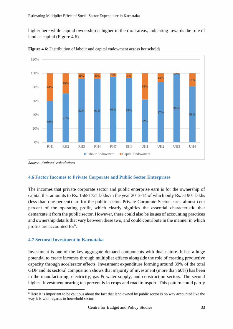
Estimating Multiplier Effect of Social Sector Expenditure in Karnataka
Centre for Budget and Policy Studies 33
higher here while capital ownership is higher in the rural areas, indicating towards the role of
land as capital (Figure 4.6).
Figure 4.6: Distribution of labour and capital endowment across households
Source: Authors’ calculations
4.6 Factor Incomes to Private Corporate and Public Sector Enterprises
The incomes that private corporate sector and public enterprise earn is for the ownership of
capital that amounts to Rs. 15681721 lakhs in the year 2013-14 of which only Rs. 51901 lakhs
(less than one percent) are for the public sector. Private Corporate Sector earns almost cent
percent of the operating profit, which clearly signifies the essential characteristic that
demarcate it from the public sector. However, there could also be issues of accounting practices
and ownership details that vary between these two, and could contribute in the manner in which
profits are accounted for6.
4.7 Sectoral Investment in Karnataka
Investment is one of the key aggregate demand components with dual nature. It has a huge
potential to create incomes through multiplier effects alongside the role of creating productive
capacity through accelerator effects. Investment expenditure forming around 39% of the total
GDP and its sectoral composition shows that majority of investment (more than 60%) has been
in the manufacturing, electricity, gas & water supply, and construction sectors. The second
highest investment nearing ten percent is in crops and road transport. This pattern could partly
6 Here it is important to be cautious about the fact that land owned by public sector is no way accounted like the
way it is with regards to household sector.
60%
71%
92% 92% 95% 93%
62%
87%
99%
81%
40%
29%
8% 8% 5% 7%
38%
13%
1%
19%
0%
20%
40%
60%
80%
100%
120%
RH1 RH2 RH3 RH4 RH5 RH6 UH1 UH2 UH3 UH4
Labour Endowment Capital Endowment
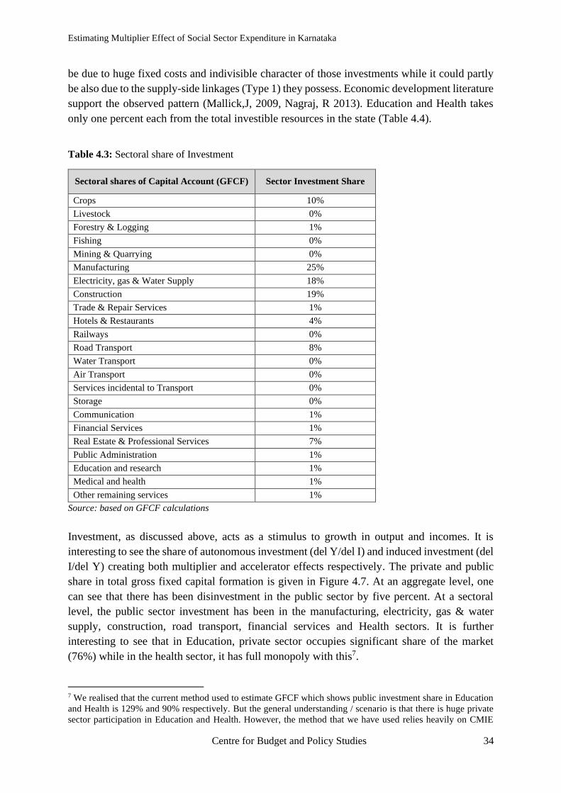
Estimating Multiplier Effect of Social Sector Expenditure in Karnataka
Centre for Budget and Policy Studies 34
be due to huge fixed costs and indivisible character of those investments while it could partly
be also due to the supply-side linkages (Type 1) they possess. Economic development literature
support the observed pattern (Mallick,J, 2009, Nagraj, R 2013). Education and Health takes
only one percent each from the total investible resources in the state (Table 4.4).
Table 4.3: Sectoral share of Investment
Sectoral shares of Capital Account (GFCF) Sector Investment Share
Crops 10%
Livestock 0%
Forestry & Logging 1%
Fishing 0%
Mining & Quarrying 0%
Manufacturing 25%
Electricity, gas & Water Supply 18%
Construction 19%
Trade & Repair Services 1%
Hotels & Restaurants 4%
Railways 0%
Road Transport 8%
Water Transport 0%
Air Transport 0%
Services incidental to Transport 0%
Storage 0%
Communication 1%
Financial Services 1%
Real Estate & Professional Services 7%
Public Administration 1%
Education and research 1%
Medical and health 1%
Other remaining services 1%
Source: based on GFCF calculations
Investment, as discussed above, acts as a stimulus to growth in output and incomes. It is
interesting to see the share of autonomous investment (del Y/del I) and induced investment (del
I/del Y) creating both multiplier and accelerator effects respectively. The private and public
share in total gross fixed capital formation is given in Figure 4.7. At an aggregate level, one
can see that there has been disinvestment in the public sector by five percent. At a sectoral
level, the public sector investment has been in the manufacturing, electricity, gas & water
supply, construction, road transport, financial services and Health sectors. It is further
interesting to see that in Education, private sector occupies significant share of the market
(76%) while in the health sector, it has full monopoly with this7.
7 We realised that the current method used to estimate GFCF which shows public investment share in Education
and Health is 129% and 90% respectively. But the general understanding / scenario is that there is huge private
sector participation in Education and Health. However, the method that we have used relies heavily on CMIE

Estimating Multiplier Effect of Social Sector Expenditure in Karnataka
Centre for Budget and Policy Studies 35
Figure 4.7: Sectoral share of investment between public and private sectors
Source: Authors’ calculations
4.8 Savings
It is observed that the total savings of the state mobilised by various institutions amount to
23263883.7 rupees lakhs. Out of the gross savings, Private Corporate Sector does the highest
with 64% followed by foreign savings and then, household savings. Government sector
dissaved by 7% in the year 2013-14.
4.9 Direct and Indirect Tax Share
Karnataka is one of the states to have the highest tax raising capacity in the country. The direct
taxes in Karnataka amount to 5976980 rupees lakhs while Total indirect taxes amount to
8685138 rupees lakhs with 40% and 60% share respectively. But the government also provides
subsidies to incentivise certain production activities. So, the total net indirect taxes (Indirect
Taxes - Subsidies) would amount to 5802565 Rupees Lakhs.
4.10 Analyses of Multipliers
4.10.1 Linkages
Theoretically, the linkages assist in sectoral allocation of resources and growth promotion. For
a sector, the proportion of the cost of intermediate inputs to total value of output gives the
which has a small sample for Education and Heath. Hence, the source could be the reason for a different picture
for Karnataka as against what is believed
100%100%
53%46%
-6%0%
19%
35%
21%
0%9% 12%
0% 2%
92%
0% 0% 0%
100%
129%90%
49%
0% 0%
47%54%
106%100%
81%
65%
79%
100%91% 88%
100%98%
8%
100%100%100%
0%
-29%
10%
51%
-20%
0%
20%
40%
60%
80%
100%
Public Sector Share of Investment Private Sector Share of Investment
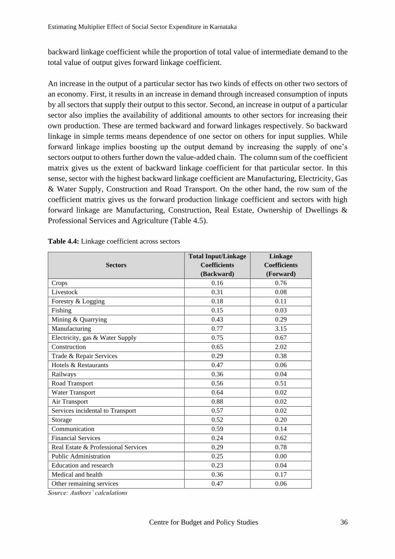
Estimating Multiplier Effect of Social Sector Expenditure in Karnataka
Centre for Budget and Policy Studies 36
backward linkage coefficient while the proportion of total value of intermediate demand to the
total value of output gives forward linkage coefficient.
An increase in the output of a particular sector has two kinds of effects on other two sectors of
an economy. First, it results in an increase in demand through increased consumption of inputs
by all sectors that supply their output to this sector. Second, an increase in output of a particular
sector also implies the availability of additional amounts to other sectors for increasing their
own production. These are termed backward and forward linkages respectively. So backward
linkage in simple terms means dependence of one sector on others for input supplies. While
forward linkage implies boosting up the output demand by increasing the supply of one’s
sectors output to others further down the value-added chain. The column sum of the coefficient
matrix gives us the extent of backward linkage coefficient for that particular sector. In this
sense, sector with the highest backward linkage coefficient are Manufacturing, Electricity, Gas
& Water Supply, Construction and Road Transport. On the other hand, the row sum of the
coefficient matrix gives us the forward production linkage coefficient and sectors with high
forward linkage are Manufacturing, Construction, Real Estate, Ownership of Dwellings &
Professional Services and Agriculture (Table 4.5).
Table 4.4: Linkage coefficient across sectors
Sectors
Total Input/Linkage
Coefficients
(Backward)
Linkage
Coefficients
(Forward)
Crops 0.16 0.76
Livestock 0.31 0.08
Forestry & Logging 0.18 0.11
Fishing 0.15 0.03
Mining & Quarrying 0.43 0.29
Manufacturing 0.77 3.15
Electricity, gas & Water Supply 0.75 0.67
Construction 0.65 2.02
Trade & Repair Services 0.29 0.38
Hotels & Restaurants 0.47 0.06
Railways 0.36 0.04
Road Transport 0.56 0.51
Water Transport 0.64 0.02
Air Transport 0.88 0.02
Services incidental to Transport 0.57 0.02
Storage 0.52 0.20
Communication 0.59 0.14
Financial Services 0.24 0.62
Real Estate & Professional Services 0.29 0.78
Public Administration 0.25 0.00
Education and research 0.23 0.04
Medical and health 0.36 0.17
Other remaining services 0.47 0.06
Source: Authors’ calculations
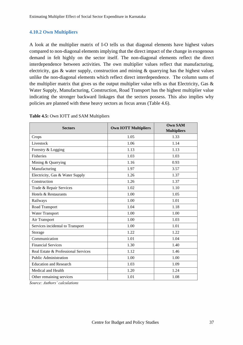
Estimating Multiplier Effect of Social Sector Expenditure in Karnataka
Centre for Budget and Policy Studies 37
4.10.2 Own Multipliers
A look at the multiplier matrix of I-O tells us that diagonal elements have highest values
compared to non-diagonal elements implying that the direct impact of the change in exogenous
demand in felt highly on the sector itself. The non-diagonal elements reflect the direct
interdependence between activities. The own multiplier values reflect that manufacturing,
electricity, gas & water supply, construction and mining & quarrying has the highest values
unlike the non-diagonal elements which reflect direct interdependence. The column sums of
the multiplier matrix that gives us the output multiplier value tells us that Electricity, Gas &
Water Supply, Manufacturing, Construction, Road Transport has the highest multiplier value
indicating the stronger backward linkages that the sectors possess. This also implies why
policies are planned with these heavy sectors as focus areas (Table 4.6).
Table 4.5: Own IOTT and SAM Multipliers
Sectors Own IOTT Multipliers Own SAM
Multipliers
Crops 1.05 1.33
Livestock 1.06 1.14
Forestry & Logging 1.13 1.13
Fisheries 1.03 1.03
Mining & Quarrying 1.16 0.93
Manufacturing 1.97 3.57
Electricity, Gas & Water Supply 1.26 1.37
Construction 1.26 1.37
Trade & Repair Services 1.02 1.10
Hotels & Restaurants 1.00 1.05
Railways 1.00 1.01
Road Transport 1.04 1.18
Water Transport 1.00 1.00
Air Transport 1.00 1.03
Services incidental to Transport 1.00 1.01
Storage 1.22 1.22
Communication 1.01 1.04
Financial Services 1.30 1.40
Real Estate & Professional Services 1.12 1.46
Public Administration 1.00 1.00
Education and Research 1.03 1.09
Medical and Health 1.20 1.24
Other remaining services 1.01 1.08
Source: Authors’ calculations

Estimating Multiplier Effect of Social Sector Expenditure in Karnataka
Centre for Budget and Policy Studies 38
4.10.3 Output Multiplier SAM and IOTT
A comparison of output multiplier of both SAM and IOTT that capture the backward
linkages/supply side effects also reflects some interesting patterns. IOTT, as it represents
production structure, shows that output multiplier effects are larger in sectors like Electricity,
Manufacturing, Construction and Mining while these are lower for Social Sectors (1.59 for
Education and 1.73 for Health). On the other hand, the SAM output multiplier effects show
that along with Manufacturing, Construction and Electricity, Education also has one of the
highest output multiplier effects. Health sector also shows a better supply side effects with the
value of 5.43. It is important to recognise that social sectors also have better supply/backward
linkages when the income distribution structure is also considered, which is what happens in
the SAM computations (Table 4.7).
Table 4.6: Output Multipliers for IOTT and SAM
Sectors Output Multiplier
SAM
Output Multiplier
IOTT
Crops 4.95 1.34
Livestock 4.93 1.70
Forestry & Logging 4.33 1.29
Fisheries 4.50 1.36
Mining & Quarrying 0.45 2.14
Manufacturing 6.73 2.88
Electricity, Gas & Water Supply 6.06 3.05
Construction 6.10 2.72
Trade & Repair Services 4.33 1.80
Hotels & Restaurants 4.75 2.01
Railways 5.38 1.92
Road Transport 5.33 2.43
Water Transport -0.42 2.67
Air Transport 37.44 3.36
Services incidental to Transport 22.24 2.10
Storage 4.76 2.08
Communication 5.26 2.20
Financial Services 4.01 1.34
Real Estate & Professional Services 4.35 1.67
Public Administration 5.76 1.61
Education and Research 6.31 1.59
Medical and Health 5.43 1.73
Other remaining services 7.43 2.20
Source: Authors’ calculations
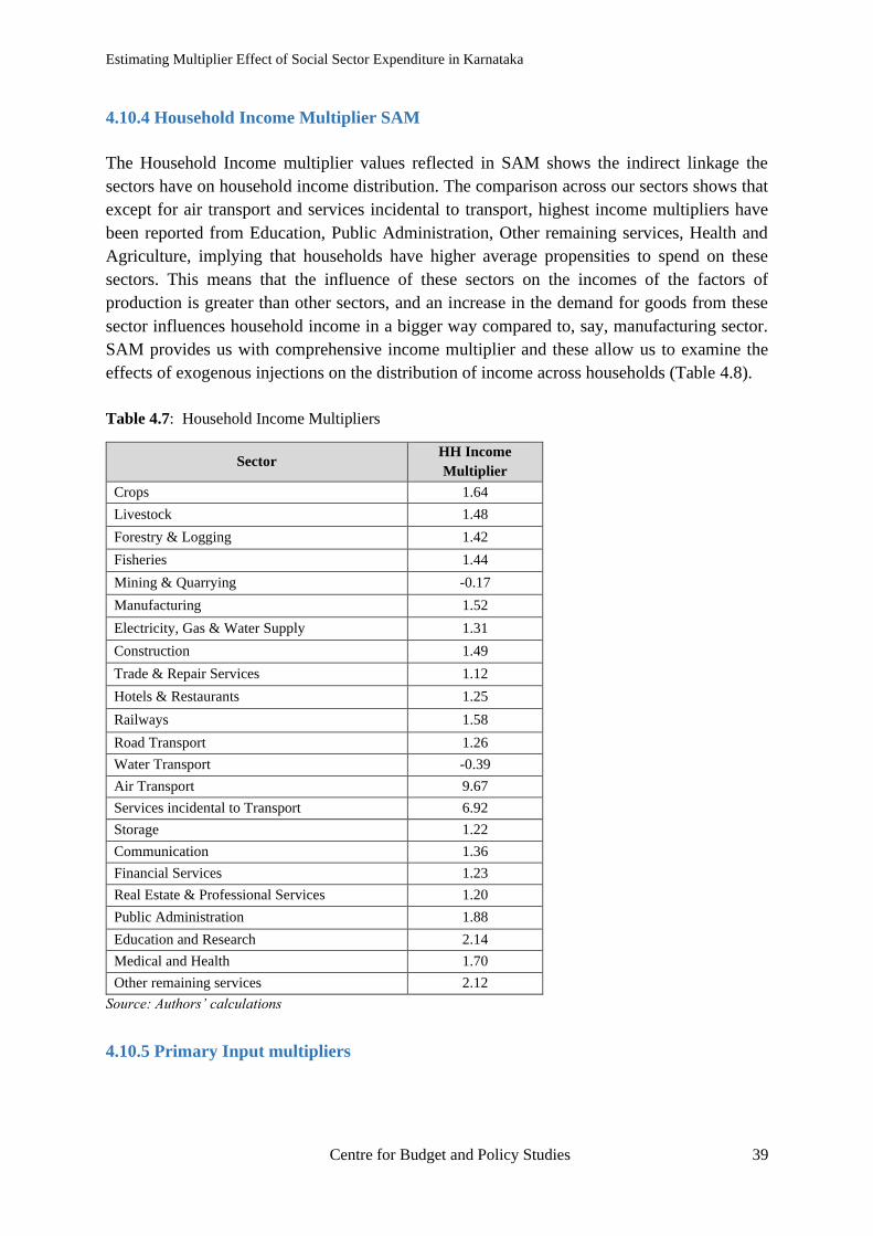
Estimating Multiplier Effect of Social Sector Expenditure in Karnataka
Centre for Budget and Policy Studies 39
4.10.4 Household Income Multiplier SAM
The Household Income multiplier values reflected in SAM shows the indirect linkage the
sectors have on household income distribution. The comparison across our sectors shows that
except for air transport and services incidental to transport, highest income multipliers have
been reported from Education, Public Administration, Other remaining services, Health and
Agriculture, implying that households have higher average propensities to spend on these
sectors. This means that the influence of these sectors on the incomes of the factors of
production is greater than other sectors, and an increase in the demand for goods from these
sector influences household income in a bigger way compared to, say, manufacturing sector.
SAM provides us with comprehensive income multiplier and these allow us to examine the
effects of exogenous injections on the distribution of income across households (Table 4.8).
Table 4.7: Household Income Multipliers
Sector HH Income
Multiplier
Crops 1.64
Livestock 1.48
Forestry & Logging 1.42
Fisheries 1.44
Mining & Quarrying -0.17
Manufacturing 1.52
Electricity, Gas & Water Supply 1.31
Construction 1.49
Trade & Repair Services 1.12
Hotels & Restaurants 1.25
Railways 1.58
Road Transport 1.26
Water Transport -0.39
Air Transport 9.67
Services incidental to Transport 6.92
Storage 1.22
Communication 1.36
Financial Services 1.23
Real Estate & Professional Services 1.20
Public Administration 1.88
Education and Research 2.14
Medical and Health 1.70
Other remaining services 2.12
Source: Authors’ calculations
4.10.5 Primary Input multipliers

Estimating Multiplier Effect of Social Sector Expenditure in Karnataka
Centre for Budget and Policy Studies 40
Primary Input Multipliers reveal that an exogenous increase in demand have highest influence
for sectors that include public administration, Education, personal and community services,
crops and health. For the remaining sectors, there is not much variation (Table 4.9).
Table 4.8: Primary Input Multipliers
Sectors Primary Input
Multipliers
Crops 2.69
Livestock 2.44
Forestry & Logging 2.33
Fisheries 2.35
Mining & Quarrying -0.30
Manufacturing 2.51
Electricity, Gas & Water Supply 2.22
Construction 2.40
Trade & Repair Services 2.05
Hotels & Restaurants 2.18
Railways 2.48
Road Transport 2.19
Water Transport -0.68
Air Transport 15.20
Services incidental to Transport 11.98
Storage 2.15
Communication 2.32
Financial Services 2.25
Real Estate & Professional Services 2.17
Public Administration 2.79
Education and Research 3.11
Medical and Health 2.58
Other remaining services 3.40
Source: Authors’ calculations
4.10.6 HH Income Multiplier across Households
The income multipliers among households turn out to be the highest for the self-employed in
both agriculture and non-agriculture in rural areas, and also in urban areas, with the lowest
multiplier value being for casual income households. This implies that growth effects are not
reaching these households and therefore they require special government intervention as
market forces are not able to trickle down its effect on these groups (Table 4.10).

Estimating Multiplier Effect of Social Sector Expenditure in Karnataka
Centre for Budget and Policy Studies 41
Table 4.9: Income Multipliers by Household Groups
HH Categories HH Income Multiplier
RH1 9.07
RH2 2.29
RH3 1.94
RH4 3.19
RH5 1.21
RH6 0.11
UH1 9.92
UH2 14.15
UH3 1.4
UH4 1.09
Source: Authors’ calculations
4.10.7 Full Income Multipliers
A submatrix in SAM reflects the Full Income Multipliers for Households where the diagonal
elements of the matrix shows the combination of direct and indirect effects of an exogenous
increase in the income of an institution working through the other accounts of SAM back to its
source. The comparison of diagonal elements reflects that regular salaried and self-employed
in urban areas, and self-employed in agriculture in rural areas benefit the most from an
exogenous increase in the income of any household group. It shows the contrast between rural
and urban sectors where rural sector except for those self-employed in agriculture, and
therefore landed, is devoid of any redistribution effects. The beneficial impact due to the
increase in the income of other household groups is clearly small (Table 4.11).
Table 4.10: Full Income Multipliers by HH Groups
Full Income Multipliers
HH Categories RH1 RH2 RH3 RH4 RH5 RH6 UH1 UH2 UH3 UH4
RH1 1.23 0.34 0.25 0.31 0.29 0.54 0.28 0.22 0.32 0.30
RH2 0.06 1.09 0.06 0.08 0.07 0.14 0.07 0.06 0.08 0.08
RH3 0.05 0.07 1.05 0.06 0.06 0.11 0.06 0.05 0.07 0.06
RH4 0.08 0.12 0.09 1.11 0.10 0.18 0.09 0.08 0.11 0.10
RH5 0.03 0.04 0.03 0.04 1.04 0.07 0.04 0.03 0.04 0.04
RH6 0.00 0.00 0.00 0.00 0.00 1.01 0.00 0.00 0.00 0.00
UH1 0.26 0.37 0.27 0.33 0.31 0.59 1.30 0.24 0.35 0.33
UH2 0.36 0.52 0.38 0.47 0.44 0.82 0.42 1.34 0.49 0.46
UH3 0.04 0.05 0.04 0.05 0.04 0.08 0.04 0.03 1.05 0.05
UH4 0.03 0.04 0.03 0.04 0.03 0.06 0.03 0.03 0.04 1.04
Source: Authors’ calculations
Estimating Multiplier Effect of Social Sector Expenditure in Karnataka
Centre for Budget and Policy Studies 42
4.10.8 Comparison of SAM and IOTT Multipliers
Estimating output and forward multipliers should be normalised as it helps us identify the key
sectors with varied potential for the economy. The normalisation was done by taking the value
of sector’s own multiplier value divided by the sum of multipliers for all the sectors, and then
normalised by 23, the number of sectors under our purview. Further, a comparison of
normalised forward and backward multiplier helps us arrive at the key sectors and their
potentials. There are four categories these sectors and their ‘key-ness’ can be classified as
follows;
Category 1: Sectors that have high forward and backward linkage effects influence both the
sector they get and take input. The sectors where both effects are high are called the key sector
or locomotive sector
Category 2: Sectors that have high backward but low forward linkage effects are the sectors
effective in the evaluation of natural resources of the country.
Category 3: Sectors that have high forward but low backward linkage effects are the sectors
producing intermediate goods and they increase the production of sectors demanding these
goods.
Category 4: Sectors that have low backward and forward linkage effects do not influence the
other sectors directly, but help to increase the country’s income by creating added value
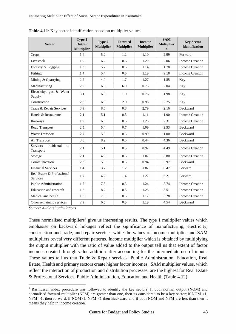
Estimating Multiplier Effect of Social Sector Expenditure in Karnataka
Centre for Budget and Policy Studies 43
Table 4.11: Key sector identification based on multiplier values
Sector
Type 1
Output
Multiplier
Type 2
Multiplier
Forward
Multiplier
Income
Multiplier
SAM
Multiplier
s
Key Sector
identification
Crops 1.4 5.2 1.2 1.10 2.99 Forward
Livestock 1.9 6.2 0.6 1.20 2.06 Income Creation
Forestry & Logging 1.3 5.7 0.5 1.14 1.78 Income Creation
Fishing 1.4 5.4 0.5 1.19 2.18 Income Creation
Mining & Quarrying 2.2 4.9 1.7 1.27 1.85 Key
Manufacturing 2.9 6.3 6.0 0.73 2.04 Key
Electricity, gas & Water
Supply 3.1 6.3 1.0 0.76 1.98 Key
Construction 2.8 6.9 2.0 0.98 2.75 Key
Trade & Repair Services 3.9 8.6 0.8 2.79 2.16 Backward
Hotels & Restaurants 2.1 5.1 0.5 1.11 1.90 Income Creation
Railways 1.9 6.6 0.5 1.25 2.31 Income Creation
Road Transport 2.5 5.4 0.7 1.09 2.53 Backward
Water Transport 2.7 5.6 0.5 0.99 1.00 Backward
Air Transport 3.5 8.2 0.5 0.44 4.36 Backward
Services incidental to
Transport 2.1 5.1 0.5 0.92 4.49 Income Creation
Storage 2.1 4.9 0.6 1.02 3.80 Income Creation
Communication 2.3 5.5 0.5 0.94 3.97 Backward
Financial Services 1.4 3.7 1.2 1.02 0.47 Forward
Real Estate & Professional
Services 1.7 4.2 1.4 1.22 6.21 Forward
Public Administration 1.7 7.8 0.5 1.24 5.74 Income Creation
Education and research 1.6 8.2 0.5 1.23 5.51 Income Creation
Medical and health 1.8 7.3 0.5 1.17 5.28 Income Creation
Other remaining services 2.2 6.5 0.5 1.19 4.54 Backward
Source: Authors’ calculations
These normalised multipliers8 give us interesting results. The type 1 multiplier values which
emphasise on backward linkages reflect the significance of manufacturing, electricity,
construction and trade, and repair services while the values of income multiplier and SAM
multipliers reveal very different patterns. Income multiplier which is obtained by multiplying
the output multiplier with the ratio of value added to the output tell us that extent of factor
incomes created through value addition after accounting for the intermediate use of inputs.
These values tell us that Trade & Repair services, Public Administration, Education, Real
Estate, Health and primary sectors create higher factor incomes. SAM multiplier values, which
reflect the interaction of production and distribution processes, are the highest for Real Estate
& Professional Services, Public Administration, Education and Health (Table 4.12).
8 Rasmussen index procedure was followed to identify the key sectors. If both normal output (NOM) and
normalised forward multiplier (NFM) are greater than one, then its considered to be a key sector; if NOM <1,
NFM >1, then forward, if NOM>1, NFM <1 then Backward and if both NOM and NFM are less than then it
means they help in income creation.

Estimating Multiplier Effect of Social Sector Expenditure in Karnataka
Centre for Budget and Policy Studies 44
The values of all kinds of multipliers estimated seem to show that Social Sector expenditure is
indeed an investment to be undertaken not only for its impact on human well-being and
productivity in the long run but also for the high potential it has for income creation in the short
run. The multiplier values show that manufacturing sector has larger backward linkage effects.
State driven social sector expenditure would enhance consumption due to extra income left in
the hands of the people and subsequently resulting in larger multiplier. In the context of
Karnataka, when more than 80 percent of the households hold Below Poverty Line cards, their
propensity to consume is higher. The interlinkage effects between sectors is a key to understand
the rationale behind the need to undertake public investment in social sector.
4.11 Policy Conclusions
Karnataka, in 2001, was one of first states in India to accept World Bank guided economic
reform at a time when state was in the midst of financial constraints to undergo economic
restructuring at the state level. New form of development, known popularly as ‘fiscalised
development’, designed largely to ‘modernise’ the state’s finances through non-state financing
and develop channels to do so. The World Bank’s Reformed Model of Development was
pursued as an alternative to state-led development. The agenda put-forth in this model gives us
a snapshot of the fiscal reform envisaged by the Bank and perhaps continues to guide the
decision making and policy choices (GoK Finance MTFP 2001). The government wanted to
withdraw itself from ‘implicit subsidies’ in secondary and tertiary healthcare services,
irrigation, and drinking water supply, higher and technical education. The immediate step
undertaken by the state to improve the fiscal base was aimed at social sectors under the rationale
of poor cost recovery. It is important to mention here that studies have long shown that
government’s support to corporate sector has played a role in establishing Bengaluru as the
Silicon Valley. These subsidies given either in form of tax cuts or other provisions do not get
classified as wasteful expenditure unlike when the same is spent on social sectors; these are
incentives and similar expenditure need to be viewed as incentives and investment elsewhere
as well. This is especially important if the state is committed to SDGs and CRC.
One of our recent studies on public expenditure on children in 16 states in India clearly revealed
a very high positive correlation between high level of public spending on education, health,
nutrition and protection and the development indicators for the same establishing the need for
public system led expansion of these sectors. States like Gujarat despite high GSDP and
capacity to spend have not been able to achieve a high progress in child development and
empowerment indicators as they have failed to invest sufficiently in public education and health
whereas states like Odisha have achieved a turnaround though its high public spending and
wise choice of policies (Jha et al, 2019). Therefore, to reiterate, since our results show that
investments in the social sectors also have positive income creation effects in Karnataka, both
from supply side and demand side even in the short run, it is therefore, imperative to enhance
social sector investment to revitalise the economy and to achieve the long-term gains of
sustainable development.
Estimating Multiplier Effect of Social Sector Expenditure in Karnataka
Centre for Budget and Policy Studies 45
Fiscal Discipline in the era of neo-liberal capitalism has become the order of the political
economy of every government of the day leading to output contraction and unemployment. IO
and SAM being robust tools in representing the interaction between economic processes and
between agents/institutions tells us how such policies guiding the current order adversely
affects the economies. The only way to pull out of this is government expenditure that can drive
the growth process.
Economic growth is usually associated with reducing structural inequalities but the evidence
across the world and especially within developing economies varied widely. The trickle-down
effect is not bound to happen is been realized lately as various features like sectoral
composition of growth, demand patterns etc., matters in reducing at least income based
deprivation. Subsequently, our study also shows how given the supply side effects the industry
sector has on other sectors of the economy, multipliers concerning the social sectors highlight
that they do have the potential to create incomes in the short run. The choice of policy
intervention differs on the type of multiplier we would like to focus on. If one emphasizes on
the distribution aspect alongside production, then social sectors have shown to have potential
in creating incomes directly in the hands of people. This is reflected in the SAM and Income
multiplier effect being greater for social sectors than manufacturing sector reflecting the
significant linkage effects of income and expenditure. Further, our study suggest that a
combination of interventions is essential to overcome structural barriers that exist between rural
and urban and between households to achieve a broad-based growth

Estimating Multiplier Effect of Social Sector Expenditure in Karnataka
Centre for Budget and Policy Studies 46
References
Data Sources
ADB, A. A., Furceri, D., & IMF, P. T. (2016). The macroeconomic effects of public
investment: Evidence from advanced economies. Journal of Macroeconomics, 50, 224-240.
Agénor, P. R., &Canuto, O. (2013). Gender equality and economic growth in Brazil: a long-
run analysis. The World Bank.
Agénor, P., &Canuto, O. (2013). Gender equality and economic growth: A framework for
policy analysis. Publicado en VOX. Disponible en http://www. voxeu. org/article/gender-
equality-and-economic-growth-framework-policyanalysis
Ahang, M. (2014). The impact of Gender inequality on Economic Growth in Developed
Countries. Advances in Environmental Biology, 8(17), 508-513.
Alesina, A., Favero, C. A., & Giavazzi, F. (2018, May). What do we know about the effects of
austerity? In AEA Papers and Proceedings (Vol. 108, pp. 524-30).
Amiri, A., &Gerdtham, U. G. (2013). Impact of maternal and child health on economic growth:
New evidence based granger causality and DEA analysis. Newborn and Child Health, Study
Commissioned by the Partnership for Maternal, Lund University, Sweden.
Annabi, N., Harvey, S., &Lan, Y. (2011). Public expenditures on education, human capital and
growth in Canada: An OLG model analysis. Journal of Policy Modeling, 33(6), 852-865.
Beraldo, S., Montolio, D., &Turati, G. (2009). Healthy, educated and wealthy: A primer on the
impact of public and private welfare expenditures on economic growth. The Journal of Socio-
Economics, 38(6), 946-956.
Bhaduri, A. (1986). Macroeconomics: the dynamics of commodity production. Springer.
Bhakta, R. (2014). Impact of public spending on health and education of children in India: A
Panel data simultaneous equation model.
Bhattacharya, T., & Rajeev, M. (2014). Identifying the High-linked Sectors for India: An
Application of Import-adjusted Domestic Input-output Matrix. Institute for Social and
Economic Change
Biswal, B., Jha, R., &Biswal, U. D. (2001). An Empirical Analysis Of The Impact Of Public
Expenditures On Education And Health On Poverty In Indian States (No. 998). Economics
Department, Queen's University.
Bloom, D. E., Canning, D., & Sevilla, J. (2004). The effect of health on economic growth: a
production function approach. World development, 32(1), 1-13.
Cassar, I. P. (2015). Estimates of output, income value added and employment multipliers for
the Maltese economy (No. WP/03/2015). Central Bank of Malta.
Centre for Budget and Governance and Accountability (2019). Numbers That Count - an
Assessment of the Union Budgets of NDA II.
Chakraborty, P. (2010). Deficit Fundamentalism vs Fiscal Federalism: Implications of 13th
Finance Commission's Recommendations. Economic and Political Weekly, 56-63.

Estimating Multiplier Effect of Social Sector Expenditure in Karnataka
Centre for Budget and Policy Studies 47
Climbing Out of Debt. Finance & Development, 55(1).
Defourny, J., & Thorbecke, E. (1984). Structural path analysis and multiplier decomposition
within a social accounting matrix framework. The Economic Journal, 94(373), 111-136.
Domański, B., & Gwosdz, K. (2010). Multiplier effects in local and regional development.
Quaestiones Geographicae, 29(2), 27-37.
Estimation Of Public And Private Investment And Consumption Of Goods And Services In
Karnataka State, DES No.12:2010, Planning Department, Government of Karnataka,
Bangalore: 2010
Expansionary Austerity New International Evidence. IMF Working Papers, 1-40.
file:///C:/Users/CBPS/Downloads/KJARecommendationonKSEP.pdf
Furceri, D., & Zdzienicka, A. (2012). The effects of social spending on economic activity:
Empirical evidence from a panel of OECD countries. Fiscal Studies, 33(1), 129-152.
Ganesh-Kumar, A., & Panda, M. (2014). State level fiscal policy choices and their impacts.
Ganesh-Kumar, A., Ghosh, B. K., Mate, K., &Rawat, P. S. Some Macroeconomic Impacts of
Different Types of Public Expenditure in India-Analysis Using a Computable General
Equilibrium Model (2017). Reserve Bank of India
Ganesh-Kumar, A., Ghosh, B., Mate, K., & Rawat, P. S. (2017). Some Macroeconomic
Impacts of Different Types of Public Expenditure in India-Analysis Using a Computable
General Equilibrium Model'. Development Research Group.
Hakura, M. D. S., Hussain, M. M., Newiak, M. M., Thakoor, V., & Yang, M. F. (2016).
Inequality, gender gaps and economic growth: Comparative evidence for sub-saharan Africa.
International Monetary Fund.
Heinz Kurz&NeriSalvadori, 2000. "'Classical' Roots of Input-Output Analysis: A Short
Account of its Long Prehistory," Economic Systems Research, Taylor & Francis Journals, vol.
12(2), pages 153-179
Hong, H., & Ahmed, S. (2009). Government spending on public goods: Evidence on growth
and poverty. Economic and Political Weekly, 102-108.
http://economia.unipv.it/pagp/pagine_personali/erossi/dottorato_svar.pdf
http://mospi.nic.in/sites/default/files/reports_and_publication/statistical_publication/National
_Accounts/SUT_Methodology_final_noteforwebsite.pdf
http://www.isec.ac.in/WP%20408%20-%20Amitabha%20Sarkar%20-%20Final.pdf.
http://www.mospi.gov.in/publication/national-accounts-statistics-2015
https://www.brookings.edu/wp-content/uploads/2016/12/201612_health-and-
morbidity.pdf,https://www.karnataka.gov.in/hfw/kannada/Documents/Karnataka_Integrated_
Public_Health_Policy_2017.PDF
https://www.business-standard.com/article/elections/karnataka-govt-s-per-capita-investment-
in-health-lowest-among-south-states-118051100163_1.html
https://www.ucl.ac.uk/~uctp041/Teaching_files/Tutorial_IRF.pdf
Estimating Multiplier Effect of Social Sector Expenditure in Karnataka
Centre for Budget and Policy Studies 48
Hughes, David W. 2003. “Policy Uses of Economic Multiplier and Impact Analysis.” Choices.
2nd Quarter: 25-30, choicesmagazine.org.
Ianchovichina, E., Estache, A., Foucart, R., Garsous, G., &Yepes, T. (2012). Job creation
through infrastructure investment in the Middle East and North Africa.
Jha, J, Madhusudan R., B.V. Sidharth S., Sowmya, J., Sushmita, M. V., Deepa, K.S., and
Abraham, S. M. (2019). Public Expenditure on Children in India, Trends and Patterns, Centre
for Budget and Policy Studies and UNICEF, India
Jones, C. (2007). Input-output multipliers, general purpose technologies, and economic
development. University of California, Berkeley, September.
Jung, H. S., & Thorbecke, E. (2003). The impact of public education expenditure on human
capital, growth, and poverty in Tanzania and Zambia: a general equilibrium approach. Journal
of Policy Modeling, 25(8), 701-725.
Kaur, G., Bordoloi, S., & Rajesh, R. (2009). An empirical investigation on the inter-sectoral
linkages in India.
Keuning, S., & Thorbecke, E. (1992). The Social Accounting Matrix and Adjustment Policies:
the impact of budget retrenchment on income distribution. Adjustment and Equity in Indonesia,
OECD Development Centre, Paris.
Kim, J., Lee, J. W., & Shin, K. (2016). A model of gender inequality and economic growth.
Asian Development Bank Economics Working Paper Series, (475).
Klasen, S. (2002). Low schooling for girls, slower growth for all? Cross‐country evidence on
the effect of gender inequality in education on economic development. The World Bank
Economic Review, 16(3), 345-373.
Klasen, S., &Lamanna, F. (2009). The impact of gender inequality in education and
employment on economic growth: new evidence for a panel of countries. Feminist economics,
15(3), 91-132.
Kraay, A. (2012). How large is the government spending multiplier? Evidence from World
Bank lending. The Quarterly Journal of Economics, 127(2), 829-887.
Mahrous, W. (2016). Dynamic Impacts of Changes in Government Spending on Economic
Growth in Kenya: A Structural VAR Analysis.
Mallick, J. (2009). Trends and patterns of private investment in India. Institute for Social and
Economic Change.
Marcuzzo, M. C. (2005). Keynes and the welfare state. Elérhető: www. ie. ufrj.
br/eventos/seminarios/pesquisa/texto_02_12. pdf [Letöltve: 2017-01-09].
Mendez-Parra, M. (2015). Using a social accounting matrix to calculate output and
employment effects in Tanzania. Supporting Economic Transformation.
Micek, G. (2011). Spatial problems of estimating multiplier effects in the local scale.
Miller, R. E., & Blair, P. D. (2009). Input-output analysis: foundations and extensions.
Cambridge university press.
Miller, R. E., & Blair, P. D. (2009). Input-output analysis: foundations and extensions.
Cambridge university press.

Estimating Multiplier Effect of Social Sector Expenditure in Karnataka
Centre for Budget and Policy Studies 49
Myrdal, G.,1957, pp. 12–13 Economic Theory and Underdeveloped Regions, London:
University Paperbacks, Methuen)
Nagaraj, R. (2013). India's dream run, 2003-08: Understanding the boom and Its aftermath.
Economic and Political Weekly, 39-51.
Nooruddin, i. & Simmons, J. (2006). The Politics of hard Choices: IMP Programms and
Government Spending. International Organization, 60 (4), 1001-1033.
Doi:10.1017/S0020818306060334
Nooruddin, I., & Simmons, J. W. (2006). The politics of hard choices: IMF programs and
government spending. International Organization, 1001-1033.
Ojha, V., Pal, B., Pohit, S., & Roy, J. (2009). Social accounting matrix for India. Available at
SSRN 1457628.
Pal, B. D., & Bandarlage, J. S. (2017). Value-added disaggregated social accounting matrix for
the Indian economy of the year 2007–2008. Journal of Economic Structures, 6(1), 14.
Patnaik, U., &Patnaik, P. (2015). Imperialism in the Era of Globalization. Monthly Review,
67(3), 68. https://monthlyreview.org/2015/07/01/imperialism-in-the-era-of-globalization/
Pereira, A. M., &Andraz, J. M. (2015). On the Long-Term Macroeconomic Effects of Social
Security Spending: Evidence for 12 EU Countries. Journal of International Business and
Economics, 3(2), 63-78.
Pescatori, A., Leigh, M. D., Guajardo, J., & Devries, M. P. (2011). A new action-based dataset
of fiscal consolidation (No. 11-128). International Monetary Fund.
Powell, M., & Round, J. I. (2000). Structure and linkage in the economy of Ghana: A SAM
approach. Economic reforms in Ghana: miracle or mirage, 68-87.
Pradhan, B K, M R Saluja and S K Singh (2006). Social Accounting Matrix for India: Concepts,
Construction and Applications. New Delhi: Sage Publications
Pradhan, B. K., Saluja, M. R., & Parida, Y. (2014). A social accounting matrix for India, 2005-
06. Research in Applied Economics, 6(1), 176.
Pradhan, B. K., Saluja, M. R., Sharma, A. K., & Yadav, B. A Regional Social Accounting
Matrix for India 2007-08.
Pyatt, G., & Round, J. I. (1977). SOCIAL ACCOUNTING MATRICES FOR
DEVELOPMENT PLANNING 1. Review of Income and Wealth, 23(4), 339-364.
Pyatt, G., & Round, J. I. (1979). Accounting and fixed price multipliers in a social accounting
matrix framework. The Economic Journal, 89(356), 850-873.
Reeves, A., Basu, S., McKee, M., Meissner, C., & Stuckler, D. (2013). Does investment in the
health sector promote or inhibit economic growth?. Globalization and health, 9(1), 43.
Saikia, D (2011). Analyzing Inter-Sectoral Linkages in India. African Journal of Agricultural
Research, 6 (33): 6766-75. Sastry, D V S, B Singh, K Bhattacharya and N K Unnikrishnan
(2003). Sectoral Linkages and Growth Prospects: Reflections on the Indian Economy.
Saluja, M. R. (2014). Construction of Social Accounting Matrix for Andhra Pradesh (AP) for
2007–08. Review of Market Integration, 6(2), 175-235.
Estimating Multiplier Effect of Social Sector Expenditure in Karnataka
Centre for Budget and Policy Studies 50
Santos, S. (2018). Using a Social Accounting Matrix for analysing institutions’ income: a case
from Portugal. ASSESSMENT AND REPORTING, https://www.u-
picardie.fr/eastwest/fichiers/art225.pdf (Economidis & Economidis, 2018)
Singh, K., &Saluja, M. R. (2018). Input–Output Table for India 2013–2014: Based on the New
Series of National Accounts Statistics and Supply and the Use Table. Margin: The Journal of
Applied Economic Research, 12(2), 197-223.
Sinha, A., Siddiqui, K. A., & Sangeeta, N. (2000, August). SAM Multiplier Analysis of
Informal Households: Application to an Indian Archetype Economy. In Thirteenth
International Conference on Input-Output Techniques, Macerata, Italy, August (pp. 21-25).
Sinha, Anushree, et.al (2007): “Macro-economic database/I-O tables for three sates of India,
Uttarakhand, Jharkhand and Karnataka for revenue projection” NCAER Report submitted to
BearingPoint/USAID, (April).
Termini, V. (1981). Logical, mechanical and historical time in economics.
Thorbecke, E., & Jung, H. S. (1996). A multiplier decomposition method to analyze poverty
alleviation. Journal of Development Economics, 48(2), 279-300.
Department of Economics & Statistics, Government of Karnataka
(2017) DES, Government of Karnataka. State and District Domestic Product of Karnataka –
2016-17
Directorate of Economics & Statistics (Crops)
Economic cum Purpose Classification of Karnataka State Budget, 2011-12 to 2018-19
Economic Survey of Karnataka – 2015-16
Central Statistics Office
(2015): National Accounts Statistics 2015, New Delhi, Ministry of Statistics and Programme
Implementation.
(2016): National Health Accounts Estimates for India (2013-14), National Health Systems
Resource Centre, New Delhi: Ministry of Health and Family Welfare, Government of India.
(2017) India - Household Consumer Expenditure, Type 1: July 2011 - June 2012, NSS 68th
Round National Sample Survey Office, NSSO - Ministry of Statistics & Programme
Implementation, Government of India
(2018) India - Annual Survey of Industries 2013-14, Central Statistics Office (Industrial
Statistics Wing) - Ministry of Statistics and PI, Government of India
(2018) India - Debt & Investment Visit 2, Jan - Dec 2013, NSS 70th Round, National Sample
Survey Office - M/o Statistics and Programme Implementation (MOSPI), Government of India
(GOI)
(2018) India - Debt & Investment, NSS 70th Round Visit-1: Jan - Dec 2013, National Sample
Survey Office - M/o Statistics and Programme Implementation (MOSPI), Government of India
(GOI)
Estimating Multiplier Effect of Social Sector Expenditure in Karnataka
Centre for Budget and Policy Studies 51
(2018) India - Household Consumer Expenditure, NSS 68th Round Sch1.0 Type 2 : July 2011
- June 2012, Type – 2 National Sample Survey Office, NSSO - Ministry of Statistics &
Programme Implementation, Government of India
(2018) India - Survey on Unincorporated Non-Agricultural Enterprises (Excluding
Construction) July-June 2010-11, NSS 67th Round, National Sample Survey Office, NSSO -
Ministry of Statistics & Programme Implementation, Government of India
Finance Department, Government of Karnataka
Karnataka State Budget 2015 (in electronic format)
Overview of Budget, Financial Statement, 2015
Other Sources:
(2015) Centre for Monitoring of Indian Economy Prowess Database
(2017) Dhariwal M & Acharya G.B, The Karnataka Value Added Tax Ready-Reckoner,
Karnataka Law Journal Publications
(2019) Bruhat Bengaluri Mahanagara Palike, Government of Karnataka. Audited Accounts of
BBMP
(2019) Karnataka Municipal Data Society. Accounts of Urban Local Bodies (in electronic
format)
(2019) Karnataka State Audit & Accounts Department, Government of Karnataka. Audited
Accounts of Gram Panchayats (in electronic form)
Annual Reports of Public Sector Corporations, Public Universities, Public Hospitals

Estimating Multiplier Effect of Social Sector Expenditure in Karnataka
Centre for Budget and Policy Studies 52
Annexures
Annexure 1: The Accounts of Social Accounting Matrix (SAM)
1. Production activities: The production account in SAM is represented by Input Output Table
that captures the origin (producing sectors) and the destination of those commodities used as
inputs in consuming sectors. The rows of the matrix in this account records payments at market
prices for economic activity of producing goods and services, i.e., the row accounts show how
commodities are distributed between intermediate input demand and final demand. The column
of the production accounts records expenditure on purchase of raw materials for producing
output, expenses made on taxes imposed on intermediate purchases (indirect taxes) and
expenses on imports. The row total amounts to Aggregate Demand while the column total
records Aggregate Supply which is made up of both domestically produced goods and imports.
2. Factors of production: The factors primarily refer to labour and capital in this case who
earn incomes from employment in domestic production activities. The row in the factor
accounts records receipts for the factor services that make up the total value added and the
income factors receive from rest of the world. The column in the factor accounts refers to
expenditure made as payments by household account, private corporate sector, public
corporations and government for labour and capital services (both domestic and foreign). Here
one can disaggregate labour and capital accounts into segmentation as it has structural
consequences.
3. Institutions: The economic agents (institutions) include households, private corporate
sector, public corporations, and government. The accounts of these institutions in the row
represent the income while on the column side there is expenditure incurred by those economic
agents.
3.1 Households: The row in Households account records income received by households from
their endowments, government transfers, and external world. The column in the Households
account on the other hand captures households’ expenditure for the purpose of consumption,
income tax paid to government and indirect taxes paid on purchases and finally savings made
of the income. This account can be used further for disaggregation to show income distribution,
and therefore to show the within-group characteristics of poverty and inequality.
3.2 Private Corporate Sector: The other institution is Private Corporate Sector whose row
account records receipts to their services in the form of operating profits for factor services,
and interest paid by government. The column of Private Corporate sector account records
expenditure made by the sector towards payment of corporate taxes and resources allocated for
savings. The row total of this institution captures Income of Private Corporations while the
column total captures the usage of this income.

Estimating Multiplier Effect of Social Sector Expenditure in Karnataka
Centre for Budget and Policy Studies 53
3.3 Public Sector Corporations: The row account records the income in the form of operating
surplus while the column account captures the public sector savings.
3.4 Government: The row records receipts from various sources like Households, factors,
Private Corporate Sector, Public Sector in the form of taxes while the column account records
the expenditure incurred by the government towards consumption, interest payments, transfers,
and savings. The row total captures the total government earnings while the column total
presents the aggregate government expenditure.
4. Net Indirect taxes: This column captures the indirect tax structure and subsidies given to
sectors.
5. Capital Account: This account represents the aggregate capital account of all institutions in
the economy. It defines the savings and investment or accumulation account of the economy.
The row of capital account captures the receipts in the form of savings mobilised by
Households, Public Sector, Private Corporate Sector, Government and savings done by the
external sector. The column records the allocation of resources for capital formation or
investment across sectors and taxes on investment goods.
6. Rest of the World (ROW): The row account of ROW records income receipts by ROW
done towards imports in the form of foreign exchange payments while the column of ROW
captures expenditure incurred by the external sector towards exports, current and capital
transfers, taxes on exports and foreign savings that totals foreign exchange receipts.
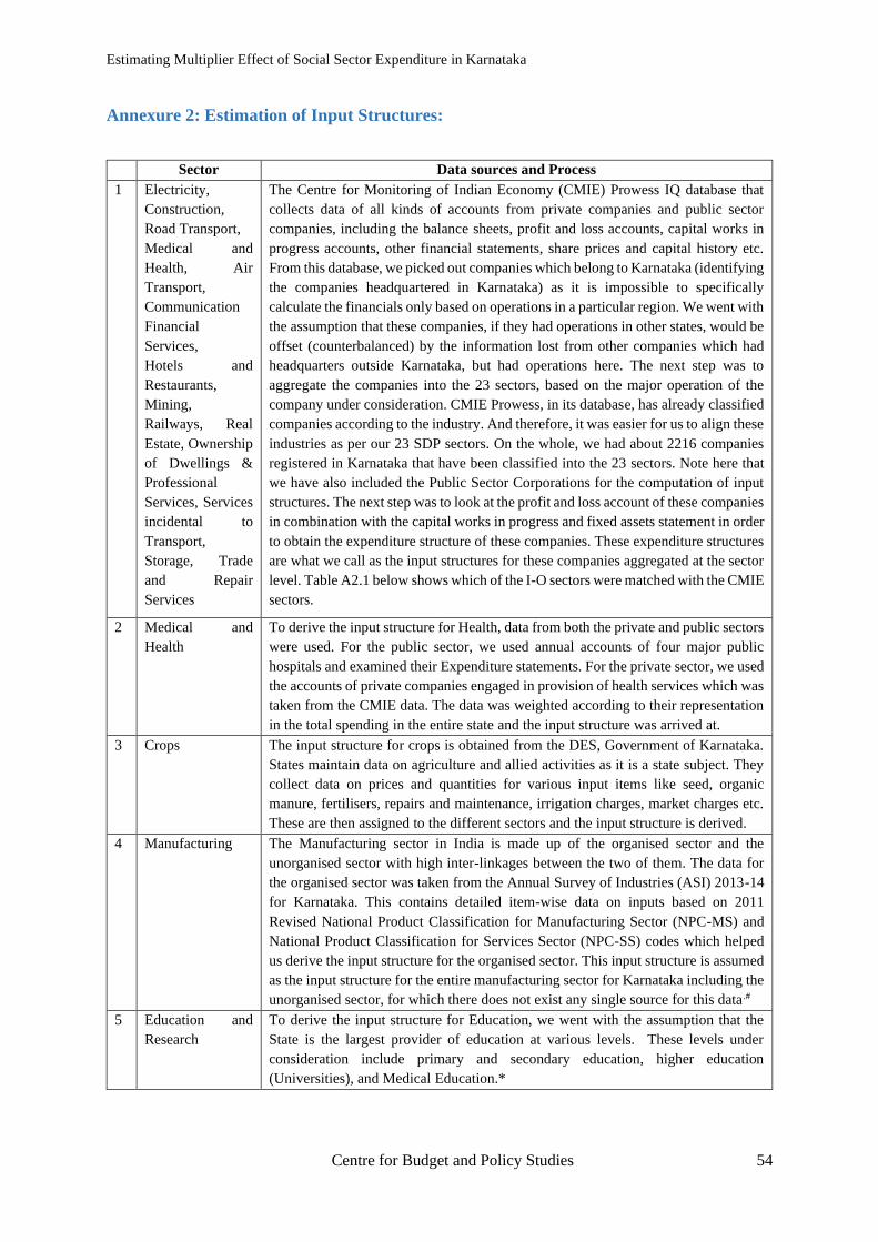
Estimating Multiplier Effect of Social Sector Expenditure in Karnataka
Centre for Budget and Policy Studies 54
Annexure 2: Estimation of Input Structures:
Sector Data sources and Process
1 Electricity,
Construction,
Road Transport,
Medical and
Health, Air
Transport,
Communication
Financial
Services,
Hotels and
Restaurants,
Mining,
Railways, Real
Estate, Ownership
of Dwellings &
Professional
Services, Services
incidental to
Transport,
Storage, Trade
and Repair
Services
The Centre for Monitoring of Indian Economy (CMIE) Prowess IQ database that
collects data of all kinds of accounts from private companies and public sector
companies, including the balance sheets, profit and loss accounts, capital works in
progress accounts, other financial statements, share prices and capital history etc.
From this database, we picked out companies which belong to Karnataka (identifying
the companies headquartered in Karnataka) as it is impossible to specifically
calculate the financials only based on operations in a particular region. We went with
the assumption that these companies, if they had operations in other states, would be
offset (counterbalanced) by the information lost from other companies which had
headquarters outside Karnataka, but had operations here. The next step was to
aggregate the companies into the 23 sectors, based on the major operation of the
company under consideration. CMIE Prowess, in its database, has already classified
companies according to the industry. And therefore, it was easier for us to align these
industries as per our 23 SDP sectors. On the whole, we had about 2216 companies
registered in Karnataka that have been classified into the 23 sectors. Note here that
we have also included the Public Sector Corporations for the computation of input
structures. The next step was to look at the profit and loss account of these companies
in combination with the capital works in progress and fixed assets statement in order
to obtain the expenditure structure of these companies. These expenditure structures
are what we call as the input structures for these companies aggregated at the sector
level. Table A2.1 below shows which of the I-O sectors were matched with the CMIE
sectors.
2 Medical and
Health
To derive the input structure for Health, data from both the private and public sectors
were used. For the public sector, we used annual accounts of four major public
hospitals and examined their Expenditure statements. For the private sector, we used
the accounts of private companies engaged in provision of health services which was
taken from the CMIE data. The data was weighted according to their representation
in the total spending in the entire state and the input structure was arrived at.
3 Crops
The input structure for crops is obtained from the DES, Government of Karnataka.
States maintain data on agriculture and allied activities as it is a state subject. They
collect data on prices and quantities for various input items like seed, organic
manure, fertilisers, repairs and maintenance, irrigation charges, market charges etc.
These are then assigned to the different sectors and the input structure is derived.
4 Manufacturing
The Manufacturing sector in India is made up of the organised sector and the
unorganised sector with high inter-linkages between the two of them. The data for
the organised sector was taken from the Annual Survey of Industries (ASI) 2013-14
for Karnataka. This contains detailed item-wise data on inputs based on 2011
Revised National Product Classification for Manufacturing Sector (NPC-MS) and
National Product Classification for Services Sector (NPC-SS) codes which helped
us derive the input structure for the organised sector. This input structure is assumed
as the input structure for the entire manufacturing sector for Karnataka including the
unorganised sector, for which there does not exist any single source for this data .#
5 Education and
Research
To derive the input structure for Education, we went with the assumption that the
State is the largest provider of education at various levels. These levels under
consideration include primary and secondary education, higher education
(Universities), and Medical Education.*
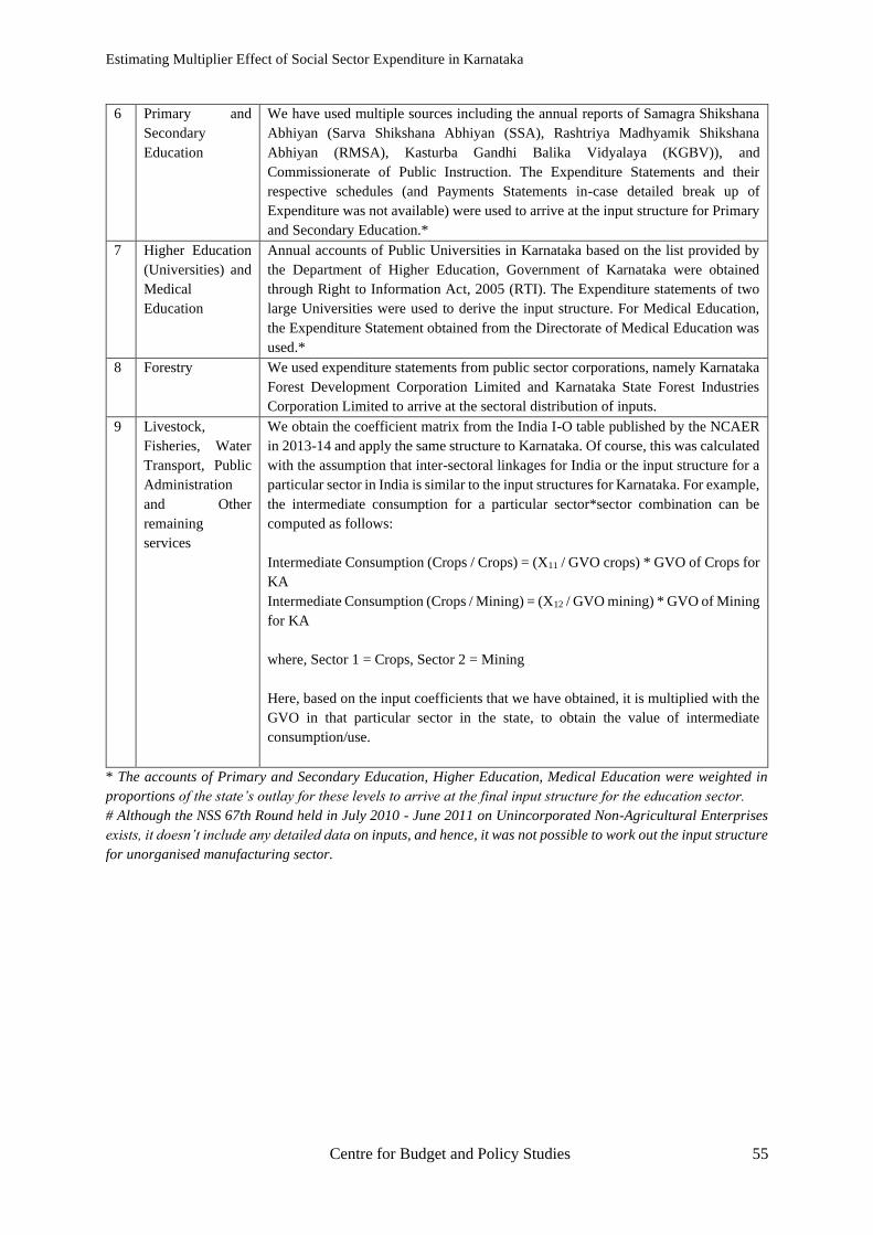
Estimating Multiplier Effect of Social Sector Expenditure in Karnataka
Centre for Budget and Policy Studies 55
6 Primary and
Secondary
Education
We have used multiple sources including the annual reports of Samagra Shikshana
Abhiyan (Sarva Shikshana Abhiyan (SSA), Rashtriya Madhyamik Shikshana
Abhiyan (RMSA), Kasturba Gandhi Balika Vidyalaya (KGBV)), and
Commissionerate of Public Instruction. The Expenditure Statements and their
respective schedules (and Payments Statements in-case detailed break up of
Expenditure was not available) were used to arrive at the input structure for Primary
and Secondary Education.*
7 Higher Education
(Universities) and
Medical
Education
Annual accounts of Public Universities in Karnataka based on the list provided by
the Department of Higher Education, Government of Karnataka were obtained
through Right to Information Act, 2005 (RTI). The Expenditure statements of two
large Universities were used to derive the input structure. For Medical Education,
the Expenditure Statement obtained from the Directorate of Medical Education was
used.*
8 Forestry We used expenditure statements from public sector corporations, namely Karnataka
Forest Development Corporation Limited and Karnataka State Forest Industries
Corporation Limited to arrive at the sectoral distribution of inputs.
9 Livestock,
Fisheries, Water
Transport, Public
Administration
and Other
remaining
services
We obtain the coefficient matrix from the India I-O table published by the NCAER
in 2013-14 and apply the same structure to Karnataka. Of course, this was calculated
with the assumption that inter-sectoral linkages for India or the input structure for a
particular sector in India is similar to the input structures for Karnataka. For example,
the intermediate consumption for a particular sector*sector combination can be
computed as follows:
Intermediate Consumption (Crops / Crops) = (X11 / GVO crops) * GVO of Crops for
KA
Intermediate Consumption (Crops / Mining) = (X12 / GVO mining) * GVO of Mining
for KA
where, Sector 1 = Crops, Sector 2 = Mining
Here, based on the input coefficients that we have obtained, it is multiplied with the
GVO in that particular sector in the state, to obtain the value of intermediate
consumption/use.
* The accounts of Primary and Secondary Education, Higher Education, Medical Education were weighted in
proportions of the state’s outlay for these levels to arrive at the final input structure for the education sector.
# Although the NSS 67th Round held in July 2010 - June 2011 on Unincorporated Non-Agricultural Enterprises
exists, it doesn’t include any detailed data on inputs, and hence, it was not possible to work out the input structure
for unorganised manufacturing sector.
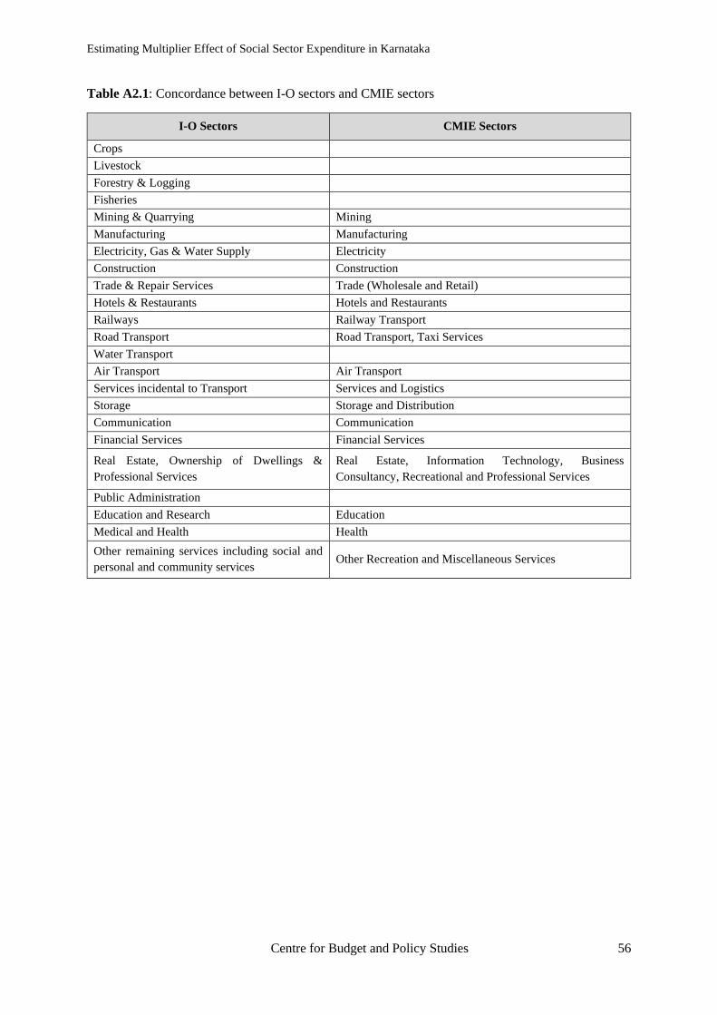
Estimating Multiplier Effect of Social Sector Expenditure in Karnataka
Centre for Budget and Policy Studies 56
Table A2.1: Concordance between I-O sectors and CMIE sectors
I-O Sectors CMIE Sectors
Crops
Livestock
Forestry & Logging
Fisheries
Mining & Quarrying Mining
Manufacturing Manufacturing
Electricity, Gas & Water Supply Electricity
Construction Construction
Trade & Repair Services Trade (Wholesale and Retail)
Hotels & Restaurants Hotels and Restaurants
Railways Railway Transport
Road Transport Road Transport, Taxi Services
Water Transport
Air Transport Air Transport
Services incidental to Transport Services and Logistics
Storage Storage and Distribution
Communication Communication
Financial Services Financial Services
Real Estate, Ownership of Dwellings &
Professional Services
Real Estate, Information Technology, Business
Consultancy, Recreational and Professional Services
Public Administration
Education and Research Education
Medical and Health Health
Other remaining services including social and
personal and community services Other Recreation and Miscellaneous Services
Estimating Multiplier Effect of Social Sector Expenditure in Karnataka
Centre for Budget and Policy Studies 57

Estimating Multiplier Effect of Social Sector Expenditure in Karnataka
Centre for Budget and Policy Studies 58
Annexure 3: Computation of Final Demand Components
Gross Value Added (GVA):
This component of the I-O table represents the total final demand in the economy. It is
equivalent to Gross State Domestic Product which explains the aggregate value of all final
goods and services produced in the year at market prices. This is the exogenous component of
the table. The GVA figures are obtained easily by Department of Economics & Statistics for
each of the 23 sectors. The data was provided to us at both basic and market prices but we have
used the data available at basic prices as the entire I-O table is computed at basic prices. The
components of the GVA include Private Final Consumption Expenditure (PFCE), Government
Final Consumption Expenditure (GFCE), Gross Fixed Capital Formation (GFCF), Net Exports
(Exports – Imports).
The individual components of the GVA were computed by exploring multiple data sources.
The main data sources used for the computation of final demand components are given below;
Sources Description
NSS 68th Round
on Household
Consumption of
Various Goods and
Services in India
This survey was conducted during the period July 2011 – June 2012 to capture the
expenditure incurred by a household for private domestic consumption for different
reference periods (7 day, 30 day or 365 day period).
Annual Survey of
Industries (ASI):
The ASI gives us the industrial statistics for India for the registered manufacturing sector.
This survey is conducted by the Central Statistics Office (CSO) and provides disaggregated
data on costs, investment, production, employment etc., by each of the manufacturing
sectors. This data was used to derive the value of inputs and the input structure for the
manufacturing sector. This is for the organised sector only.
Karnataka State
Budgets
We referred to the Budget of 2015 which contains actuals for financial year 2013-14. This
captures the detailed capital and revenue expenditure undertaken across all Administrative
Departments and Departmental Commercial Undertakings (DCUs).
Local Budgets Although the State Budgets contains data on the transfers to the Rural Local Bodies and
Urban Local Bodies, it does not capture the own sources of revenue and the detailed
expenditure across different functions by these bodies. Hence, a detailed analysis of the local
accounts is required to understand the different categories of expenditure incurred. We
procured the Consolidated Annual Audited Accounts from the State Audit and Accounts
Department (SAAD) for the year 2013-14 for all the Gram Panchayats (GP). For the Taluk
Panchayat (TP) and Zilla Panchayats (ZP), due to difficulty in accessing of data, State
Budgets were used. It is important to note that unlike GPs, these two tiers do not have any
major sources of own revenue.
For the Urban Local Bodies, detailed accounts were obtained from the Karnataka Municipal
Data Society. In addition, accounts of the Bruhat Bengaluru Mahanagara Palike (BBMP)
were added to the above to get the overall picture of ULBs in the State
Public Sector
Corporations
These are autonomous bodies under the State that function independently by generating their
own sources of revenue with additional grants from the State Government. Based on the list
of Public Sector Undertakings provided by the Department of Public Enterprises,
Government of Karnataka, we obtained the Annual Accounts of these Corporations. Some
of these accounts were obtained through RTI. To account for the data from these
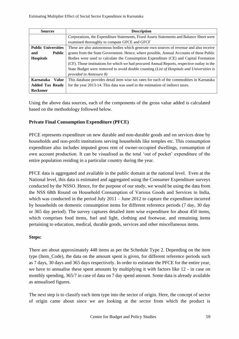
Estimating Multiplier Effect of Social Sector Expenditure in Karnataka
Centre for Budget and Policy Studies 59
Sources Description
Corporations, the Expenditure Statements, Fixed Assets Statements and Balance Sheet were
examined thoroughly to compute GFCE and GFCF
Public Universities
and Public
Hospitals
These are also autonomous bodies which generate own sources of revenue and also receive
grants from the State Government. Hence, where possible, Annual Accounts of these Public
Bodies were used to calculate the Consumption Expenditure (CE) and Capital Formation
(CF). Those institutions for which we had procured Annual Reports, respective outlay in the
State Budget were removed to avoid double counting (List of Hospitals and Universities is
provided in Annexure 8)
Karnataka Value
Added Tax Ready
Reckoner
This database provides detail item wise tax rates for each of the commodities in Karnataka
for the year 2013-14. This data was used in the estimation of indirect taxes.
Using the above data sources, each of the components of the gross value added is calculated
based on the methodology followed below.
Private Final Consumption Expenditure (PFCE)
PFCE represents expenditure on new durable and non-durable goods and on services done by
households and non-profit institutions serving households like temples etc. This consumption
expenditure also includes imputed gross rent of owner-occupied dwellings, consumption of
own account production. It can be visualised as the total ‘out of pocket’ expenditure of the
entire population residing in a particular country during the year.
PFCE data is aggregated and available in the public domain at the national level. Even at the
National level, this data is estimated and aggregated using the Consumer Expenditure surveys
conducted by the NSSO. Hence, for the purpose of our study, we would be using the data from
the NSS 68th Round on Household Consumption of Various Goods and Services in India,
which was conducted in the period July 2011 – June 2012 to capture the expenditure incurred
by households on domestic consumption items for different reference periods (7 day, 30 day
or 365 day period). The survey captures detailed item wise expenditure for about 450 items,
which comprises food items, fuel and light, clothing and footwear, and remaining items
pertaining to education, medical, durable goods, services and other miscellaneous items.
Steps:
There are about approximately 448 items as per the Schedule Type 2. Depending on the item
type (Item_Code), the data on the amount spent is given, for different reference periods such
as 7 days, 30 days and 365 days respectively. In order to estimate the PFCE for the entire year,
we have to annualise these spent amounts by multiplying it with factors like 12 - in case on
monthly spending, 365/7 in case of data on 7 day spend amount. Some data is already available
as annualised figures.
The next step is to classify each item type into the sector of origin. Here, the concept of sector
of origin came about since we are looking at the sector from which the product is
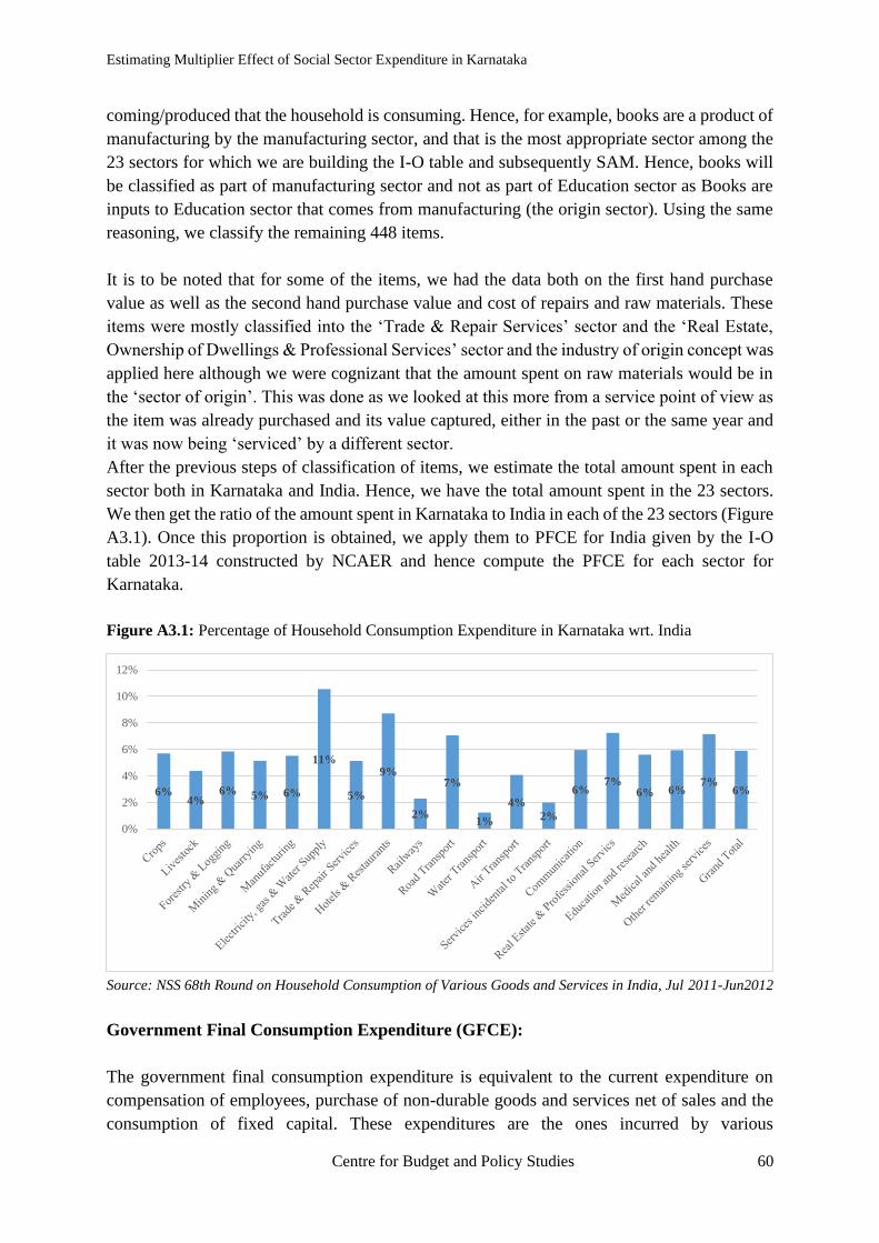
Estimating Multiplier Effect of Social Sector Expenditure in Karnataka
Centre for Budget and Policy Studies 60
coming/produced that the household is consuming. Hence, for example, books are a product of
manufacturing by the manufacturing sector, and that is the most appropriate sector among the
23 sectors for which we are building the I-O table and subsequently SAM. Hence, books will
be classified as part of manufacturing sector and not as part of Education sector as Books are
inputs to Education sector that comes from manufacturing (the origin sector). Using the same
reasoning, we classify the remaining 448 items.
It is to be noted that for some of the items, we had the data both on the first hand purchase
value as well as the second hand purchase value and cost of repairs and raw materials. These
items were mostly classified into the ‘Trade & Repair Services’ sector and the ‘Real Estate,
Ownership of Dwellings & Professional Services’ sector and the industry of origin concept was
applied here although we were cognizant that the amount spent on raw materials would be in
the ‘sector of origin’. This was done as we looked at this more from a service point of view as
the item was already purchased and its value captured, either in the past or the same year and
it was now being ‘serviced’ by a different sector.
After the previous steps of classification of items, we estimate the total amount spent in each
sector both in Karnataka and India. Hence, we have the total amount spent in the 23 sectors.
We then get the ratio of the amount spent in Karnataka to India in each of the 23 sectors (Figure
A3.1). Once this proportion is obtained, we apply them to PFCE for India given by the I-O
table 2013-14 constructed by NCAER and hence compute the PFCE for each sector for
Karnataka.
Figure A3.1: Percentage of Household Consumption Expenditure in Karnataka wrt. India
Source: NSS 68th Round on Household Consumption of Various Goods and Services in India, Jul 2011-Jun2012
Government Final Consumption Expenditure (GFCE):
The government final consumption expenditure is equivalent to the current expenditure on
compensation of employees, purchase of non-durable goods and services net of sales and the
consumption of fixed capital. These expenditures are the ones incurred by various
6%4%
6% 5% 6%
11%
5%
9%
2%
7%
1%
4%
2%
6%7%
6% 6%7%
6%
0%
2%
4%
6%
8%
10%
12%
Estimating Multiplier Effect of Social Sector Expenditure in Karnataka
Centre for Budget and Policy Studies 61
administrative departments of the government including ministries and departments of the state
government, autonomous bodies under the state government, rural and urban local authorities
engaged in administration, public sector corporations, and all other such offices of the state
government involved in administration.
Karnataka publishes the Economic cum Purpose Classification of Karnataka State Budget
Report, 2011-12 to 2018-19 (ECP). This report publishes the GFCE data for the state of
Karnataka of the General Government (Administrative Departments). However, this has some
limitations. This data does not include the data for the Public Sector Corporations. It also
captures the transfers to the Local Bodies as pure transfers without classifying them as
Consumption Expenditure or Capital Expenditure. Hence, a detailed analysis of the three data
sources including General Government Budget, Local Budgets / Local Accounts and Public
Sector Corporations was explored in detail to obtain the GFCE for Karnataka.
Public Accounts:
Public Accounts are simply all accounts of all the institutions belonging to the public sector
including the State Government departments, Local Governments (Panchayat Raj Institutions
PRIs), Public Sector Corporations, Public Universities, Public Hospitals and other such public
institutions. In order to compute the Government Final Consumption Expenditure (GFCE) and
Gross Fixed Capital Formation (this includes capital formation for the entire state, including
public and private sector) we needed to go into the in-depth analyses of each category of the
above-mentioned accounts.
State Government Budgets:
Among all the government accounts, State Government Budgets form a very important source
of information on many aspects of government policy making. Budget reflects the health of the
overall economy of a state. As discussed earlier, there are many other accounts apart from
government budgets which reflect the state of public finances, for example, the local
government budgets, accounts of public sector corporations, accounts of public universities
and hospitals which, apart from receiving grants from the state budget, also generate their own
sources of revenue.
Here, we will discuss the process involved in the detailed analyses of the State Government
Budgets. The Budget data we have is a combination of the following variables: Demand
Number, Department Code, Major Head, Sub Major Head, Minor Head, Group Head, Sub
Head, Scheme Code, Description, and Object Head. Each of these heads capture some
information on the demand for grants, like, major head captures the department from which the
grant is originating, also capturing if the demand is for revenue expenditure or a capital
expenditure. The minor head represents the specific sub department/or function that the
demand for grant is. The scheme code is a 12-digit code which, as a combination indicates
specifically what kind of grant is being demanded. The object head is a 3 digit number which

Estimating Multiplier Effect of Social Sector Expenditure in Karnataka
Centre for Budget and Policy Studies 62
classifies the expenditure into the purpose/objective of spending for the particular scheme, like,
office stationery, salary etc.
Each year, the budget also gives us the Budgeted Estimates (BE) of that year, the Actuals from
two years prior to the budgeted year, and the revised estimates of the previous year. We took
the data for the actuals spent in the financial year 2013-14 from the budget of the year 2015
(which gives the BE for the year 2015-16). The next task was to classify each of the 7000
entries of scheme codes into multiple levels of classification. They are as follows:
Type of Expenditure (Revenue / Capital): This classification was mainly done to identify all
expenditures, as either some kind of consumption expenditure or capital expenditure. The
various categories into which a revenue and capital expenditure can be classified included
transfers, subsidies, purchase of goods and services, maintenance, advances, pension, interest
payments, construction of road, buildings etc. Once the expenditure was classified into various
such heads, they are further clubbed in broad categories (purpose of expenditure). Some inputs
were obtained from DES in instances where the description of the expenditure item was vague.
Type of Institution: The type of Institution is important to classify the State Government
Departments from the other public sector institutions like Public Sector Corporations, Public
Universities, Public Hospitals, Local Governments and any other Autonomous Institutions for
which we analysed the accounts separately to take care of double counting. We basically
retained only those expenditures done by the state government department after which each of
the expenditures items to the respective sectors on the concept of ‘sector of origin’.
Given below in table A3.1 is the different heads each that of the expenditures were classified
into and the amount of actual expenditure in the particular year for that head based on the
scheme codes. As can be seen, there are about approximately 7000 such combinations. As
discussed earlier, in many cases, in spite of applying the above rules for classification, it was
difficult to identify the category that the scheme code combination should belong to.
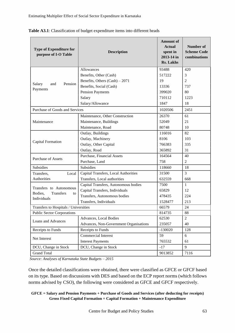
Estimating Multiplier Effect of Social Sector Expenditure in Karnataka
Centre for Budget and Policy Studies 63
Table A3.1: Classification of budget expenditure items into different heads
Type of Expenditure for
purpose of I-O Table Description
Amount of
Actual
spent in
2013-14 in
Rs. Lakhs
Number of
Scheme Code
combinations
Salary and Pension
Payments
Allowances 93488 420
Benefits, Other (Cash) 517222 3
Benefits, Others (Cash) – 2071 19 2
Benefits, Social (Cash) 13336 737
Pension Payments 399020 80
Salary 710112 1223
Salary/Allowance 1847 18
Purchase of Goods and Services 1020506 2451
Maintenance
Maintenance, Other Construction 26370 61
Maintenance, Buildings 52049 21
Maintenance, Road 80748 10
Capital Formation
Outlay, Buildings 116016 82
Outlay, Machinery 8106 103
Outlay, Other Capital 766383 335
Outlay, Road 365892 31
Purchase of Assets Purchase, Financial Assets 164564 40
Purchase, Land 758 2
Subsidies Subsidies 118660 18
Transfers, Local
Authorities
Capital Transfers, Local Authorities 31500 3
Transfers, Local authorities 632559 668
Transfers to Autonomous
Bodies, Transfers to
Individuals
Capital Transfers, Autonomous bodies 7500 1
Capital Transfers, Individuals 65829 12
Transfers, Autonomous bodies 478435 224
Transfers, Individuals 1528477 213
Transfers to Hospitals / Universities 66579 24
Public Sector Corporations 814735 88
Loans and Advances Advances, Local Bodies 62530 2
Advances, Non-Government Organisations 235057 40
Receipts to Funds Receipts to Funds -130020 128
Net Interest Commercial Interest 59 6
Interest Payments 765532 61
DCU, Change in Stock DCU, Change in Stock -17 9
Grand Total 9013852 7116
Source: Analyses of Karnataka State Budgets – 2015
Once the detailed classifications were obtained, there were classified as GFCE or GFCF based
on its type. Based on discussions with DES and based on the ECP report norms (which follows
norms advised by CSO), the following were considered as GFCE and GFCF respectively.
GFCE = Salary and Pension Payments + Purchase of Goods and Services (after deducting for receipts)
Gross Fixed Capital Formation = Capital Formation + Maintenance Expenditure
Estimating Multiplier Effect of Social Sector Expenditure in Karnataka
Centre for Budget and Policy Studies 64
Here, maintenance of buildings, other construction work and roads is considered in capital
formation as this involves some sort of ‘creation of assets’.
Local Government Accounts (Rural Local Bodies and Urban Local Bodies):
Karnataka has been one of the pioneer states in this respect with steps taken for decentralisation
setting up a three-tier system in 1987. We have now successfully established the three-tier
system of governance both in the rural local bodies (RLBs) and the urban local bodies (ULBs).
Both the RLBs and ULBs have some autonomy in term of finances. Their sources of revenue
include grants received from the state and central governments based on the ratio fixed by the
Central Finance Commission and State Finance Commission, grants under different Centrally
Sponsored and Central Sector Schemes. They generate their own sources of revenue, both non-
tax and tax in terms of building rents, user fees, etc., and property tax on properties located in
their jurisdiction.
Urban Local Bodies:
Karnataka has about 214 ULBs in the state. These include City Corporations (CC), about 8 in
number, Town Municipal Committees (TMC) (94), City Municipal Councils (CMC) (44) and
Taluk Panchayats (TP) (68). With help from the Asian Development Bank, Karnataka had
established the Karnataka Municipal Data Society (KMDS) which has the exclusive right to
maintain all kinds of records related to Urban Local Bodies including their financial statements,
demographic details of ULBs, dashboards, training modules etc. They act as a one source stop
for all the data requirements of ULBs. We visited the KMDS office to get information on the
financials of all the ULBs. Only one of the ULBs i.e. Bruhat Bengaluru Mahanagara Palike
(BBMP) maintains and gets its accounts audited separately. The data on both receipts and
expenditure was provided to us for each ULBs.
The expenditure items were classified as either capital formation or consumption expenditure
for each of the major heads. We classified this data further into the sectors in which they were
spent and these were added to the calculations of GFCE and GFCF respectively. Similarly, we
did this separately for the accounts of BBMP which we obtained from their office. Given below
in Figure A3.2 and Figure A3.3 is the distribution of consumption expenditure and capital
formation across different sectors in the urban local bodies.

Estimating Multiplier Effect of Social Sector Expenditure in Karnataka
Centre for Budget and Policy Studies 65
Figure A3.2: Percentage of spending across different categories across sectors in Urban Local Bodies
in Karnataka apart from Bruhat Bengaluru Mahanagara Palike
Source: Urban Local Bodies Audited Accounts
Figure A3.3: Consumption and Capital Formation distribution across sectors in Bruhat Bengaluru
Mahanagara Palike
Source: BBMP Audited Accounts
Rural Local Bodies:
All Gram Panchayats have to get their accounts audited by the State Audit and Accounts
Department (SAAD). Karnataka had about 5631 Gram Panchayats as of 2013-14. Apart from
these, we also have Taluk Panchayats (240) and Zilla Panchayats (30) whose accounts are
already present in the state Budget as all the funds is routed through the State treasury and they
do not generate any own sources of revenue unlike GPs.
41%
66%
83%
55%
59%
34% 4%
45%
0% 0%13%
0%
0%
20%
40%
60%
80%
100%
Construction Health Public Administration Water Supply
Consumption Expenditure Capital Formation Others
0% 0% 0% 0%15%
100%
68%
23%
100% 100% 100% 100%85%
0%
32%
77%
0%
20%
40%
60%
80%
100%
Consumption Expenditure Capital Formation
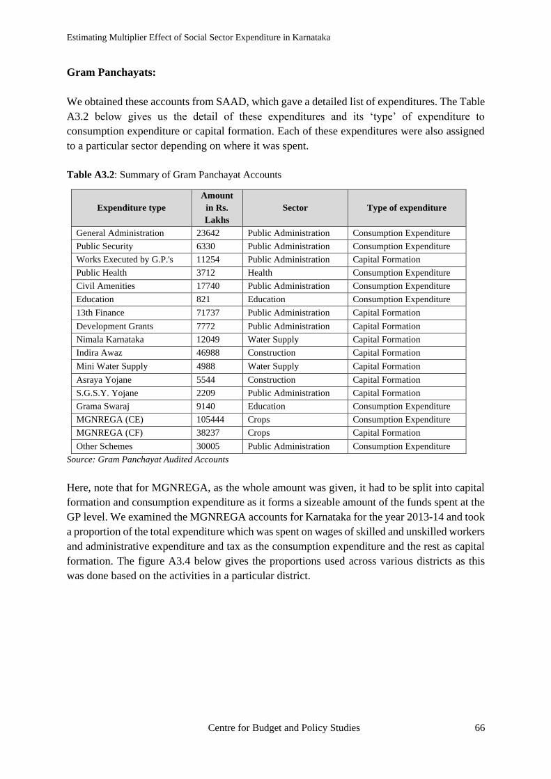
Estimating Multiplier Effect of Social Sector Expenditure in Karnataka
Centre for Budget and Policy Studies 66
Gram Panchayats:
We obtained these accounts from SAAD, which gave a detailed list of expenditures. The Table
A3.2 below gives us the detail of these expenditures and its ‘type’ of expenditure to
consumption expenditure or capital formation. Each of these expenditures were also assigned
to a particular sector depending on where it was spent.
Table A3.2: Summary of Gram Panchayat Accounts
Expenditure type
Amount
in Rs.
Lakhs
Sector Type of expenditure
General Administration 23642 Public Administration Consumption Expenditure
Public Security 6330 Public Administration Consumption Expenditure
Works Executed by G.P.'s 11254 Public Administration Capital Formation
Public Health 3712 Health Consumption Expenditure
Civil Amenities 17740 Public Administration Consumption Expenditure
Education 821 Education Consumption Expenditure
13th Finance 71737 Public Administration Capital Formation
Development Grants 7772 Public Administration Capital Formation
Nimala Karnataka 12049 Water Supply Capital Formation
Indira Awaz 46988 Construction Capital Formation
Mini Water Supply 4988 Water Supply Capital Formation
Asraya Yojane 5544 Construction Capital Formation
S.G.S.Y. Yojane 2209 Public Administration Capital Formation
Grama Swaraj 9140 Education Consumption Expenditure
MGNREGA (CE) 105444 Crops Consumption Expenditure
MGNREGA (CF) 38237 Crops Capital Formation
Other Schemes 30005 Public Administration Consumption Expenditure
Source: Gram Panchayat Audited Accounts
Here, note that for MGNREGA, as the whole amount was given, it had to be split into capital
formation and consumption expenditure as it forms a sizeable amount of the funds spent at the
GP level. We examined the MGNREGA accounts for Karnataka for the year 2013-14 and took
a proportion of the total expenditure which was spent on wages of skilled and unskilled workers
and administrative expenditure and tax as the consumption expenditure and the rest as capital
formation. The figure A3.4 below gives the proportions used across various districts as this
was done based on the activities in a particular district.

Estimating Multiplier Effect of Social Sector Expenditure in Karnataka
Centre for Budget and Policy Studies 67
Figure A3.4: Distribution of MGNREGA Proportions between Consumption Expenditure and Capital
Formation
Source: MGNREGA Accounts for Karnataka, 2013-14
Taluk Panchayats and Zilla Panchayats: The data for the Taluk and Zilla Panchayats are
given in the State Government Budgets in the link documents for each scheme code
combination that we had discussed previously in the budget section. Here again, we follow the
same method followed previously in the State Budgets analyses based on the description of the
expenditure and the major head or department which was budgeted the money to obtain
expenditures as given in Figure A3.5 below.
Figure A3.5: Proportion of Consumption Expenditure and Capital Formation in Taluk and Zilla
Panchayats
Source: Karnataka State Budgets, 2015
79%80%78%
95%
66%71%
62%
89%79%
71%
84%
70%72%74%68%67%
74%71%77%
71%74%73%78%
70%
81%71%
96%
82%73%73%73%
21%20%22%
5%
34%29%
38%
11%21%
29%
16%
30%28%26%32%33%
26%29%23%
29%26%27%22%
30%
19%29%
4%
18%27%27%27%
0%
10%
20%
30%
40%
50%
60%
70%
80%
90%
100%
Proportion of Capital FormationProportion of Consumption Expenditure (add of wage of skilled and unskilled and admn expe)
46%
1% 1% 0%14% 18%
51%
0% 0% 0%13% 7%
54%
99% 99% 100%86% 82%
49%
100% 100% 100%87% 93%
0%
20%
40%
60%
80%
100%
Consumption Expenditure Capital Formation
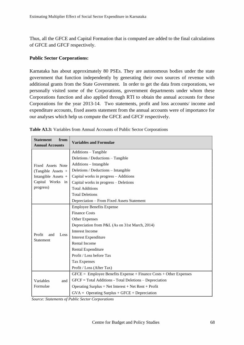
Estimating Multiplier Effect of Social Sector Expenditure in Karnataka
Centre for Budget and Policy Studies 68
Thus, all the GFCE and Capital Formation that is computed are added to the final calculations
of GFCE and GFCF respectively.
Public Sector Corporations:
Karnataka has about approximately 80 PSEs. They are autonomous bodies under the state
government that function independently by generating their own sources of revenue with
additional grants from the State Government. In order to get the data from corporations, we
personally visited some of the Corporations, government departments under whom these
Corporations function and also applied through RTI to obtain the annual accounts for these
Corporations for the year 2013-14. Two statements, profit and loss accounts/ income and
expenditure accounts, fixed assets statement from the annual accounts were of importance for
our analyses which help us compute the GFCE and GFCF respectively.
Table A3.3: Variables from Annual Accounts of Public Sector Corporations
Statement from
Annual Accounts Variables and Formulae
Fixed Assets Note
(Tangible Assets +
Intangible Assets +
Capital Works in
progress)
Additions – Tangible
Deletions / Deductions – Tangible
Additions – Intangible
Deletions / Deductions – Intangible
Capital works in progress – Additions
Capital works in progress – Deletions
Total Additions
Total Deletions
Depreciation – From Fixed Assets Statement
Profit and Loss
Statement
Employee Benefits Expense
Finance Costs
Other Expenses
Depreciation from P&L (As on 31st March, 2014)
Interest Income
Interest Expenditure
Rental Income
Rental Expenditure
Profit / Loss before Tax
Tax Expenses
Profit / Loss (After Tax)
Variables and
Formulae
GFCE = Employee Benefits Expense + Finance Costs + Other Expenses
GFCF = Total Additions - Total Deletions – Depreciation
Operating Surplus = Net Interest + Net Rent + Profit
GVA = Operating Surplus + GFCE + Depreciation
Source: Statements of Public Sector Corporations
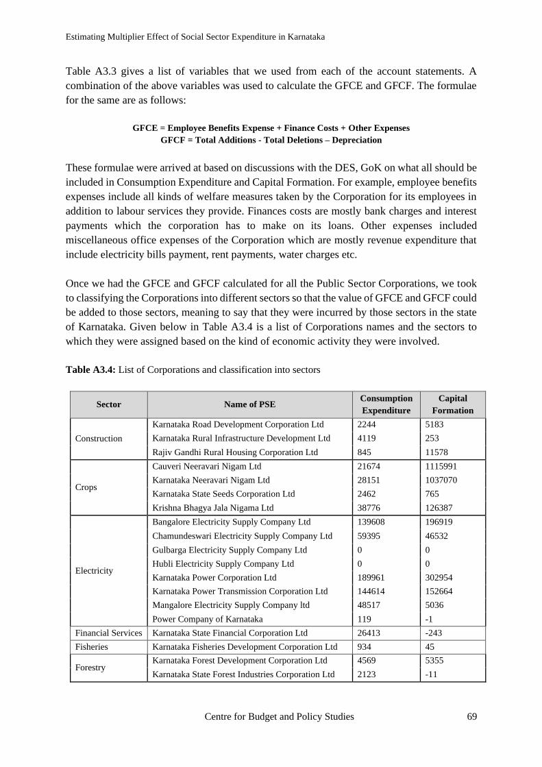
Estimating Multiplier Effect of Social Sector Expenditure in Karnataka
Centre for Budget and Policy Studies 69
Table A3.3 gives a list of variables that we used from each of the account statements. A
combination of the above variables was used to calculate the GFCE and GFCF. The formulae
for the same are as follows:
GFCE = Employee Benefits Expense + Finance Costs + Other Expenses
GFCF = Total Additions - Total Deletions – Depreciation
These formulae were arrived at based on discussions with the DES, GoK on what all should be
included in Consumption Expenditure and Capital Formation. For example, employee benefits
expenses include all kinds of welfare measures taken by the Corporation for its employees in
addition to labour services they provide. Finances costs are mostly bank charges and interest
payments which the corporation has to make on its loans. Other expenses included
miscellaneous office expenses of the Corporation which are mostly revenue expenditure that
include electricity bills payment, rent payments, water charges etc.
Once we had the GFCE and GFCF calculated for all the Public Sector Corporations, we took
to classifying the Corporations into different sectors so that the value of GFCE and GFCF could
be added to those sectors, meaning to say that they were incurred by those sectors in the state
of Karnataka. Given below in Table A3.4 is a list of Corporations names and the sectors to
which they were assigned based on the kind of economic activity they were involved.
Table A3.4: List of Corporations and classification into sectors
Sector Name of PSE Consumption
Expenditure
Capital
Formation
Construction
Karnataka Road Development Corporation Ltd 2244 5183
Karnataka Rural Infrastructure Development Ltd 4119 253
Rajiv Gandhi Rural Housing Corporation Ltd 845 11578
Crops
Cauveri Neeravari Nigam Ltd 21674 1115991
Karnataka Neeravari Nigam Ltd 28151 1037070
Karnataka State Seeds Corporation Ltd 2462 765
Krishna Bhagya Jala Nigama Ltd 38776 126387
Electricity
Bangalore Electricity Supply Company Ltd 139608 196919
Chamundeswari Electricity Supply Company Ltd 59395 46532
Gulbarga Electricity Supply Company Ltd 0 0
Hubli Electricity Supply Company Ltd 0 0
Karnataka Power Corporation Ltd 189961 302954
Karnataka Power Transmission Corporation Ltd 144614 152664
Mangalore Electricity Supply Company ltd 48517 5036
Power Company of Karnataka 119 -1
Financial Services Karnataka State Financial Corporation Ltd 26413 -243
Fisheries Karnataka Fisheries Development Corporation Ltd 934 45
Forestry Karnataka Forest Development Corporation Ltd 4569 5355
Karnataka State Forest Industries Corporation Ltd 2123 -11
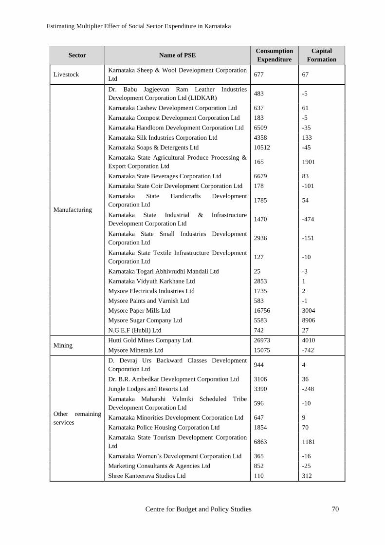
Estimating Multiplier Effect of Social Sector Expenditure in Karnataka
Centre for Budget and Policy Studies 70
Sector Name of PSE Consumption
Expenditure
Capital
Formation
Livestock Karnataka Sheep & Wool Development Corporation
Ltd 677 67
Manufacturing
Dr. Babu Jagjeevan Ram Leather Industries
Development Corporation Ltd (LIDKAR) 483 -5
Karnataka Cashew Development Corporation Ltd 637 61
Karnataka Compost Development Corporation Ltd 183 -5
Karnataka Handloom Development Corporation Ltd 6509 -35
Karnataka Silk Industries Corporation Ltd 4358 133
Karnataka Soaps & Detergents Ltd 10512 -45
Karnataka State Agricultural Produce Processing &
Export Corporation Ltd 165 1901
Karnataka State Beverages Corporation Ltd 6679 83
Karnataka State Coir Development Corporation Ltd 178 -101
Karnataka State Handicrafts Development
Corporation Ltd 1785 54
Karnataka State Industrial & Infrastructure
Development Corporation Ltd 1470 -474
Karnataka State Small Industries Development
Corporation Ltd 2936 -151
Karnataka State Textile Infrastructure Development
Corporation Ltd 127 -10
Karnataka Togari Abhivrudhi Mandali Ltd 25 -3
Karnataka Vidyuth Karkhane Ltd 2853 1
Mysore Electricals Industries Ltd 1735 2
Mysore Paints and Varnish Ltd 583 -1
Mysore Paper Mills Ltd 16756 3004
Mysore Sugar Company Ltd 5583 8906
N.G.E.F (Hubli) Ltd 742 27
Mining Hutti Gold Mines Company Ltd. 26973 4010
Mysore Minerals Ltd 15075 -742
Other remaining
services
D. Devraj Urs Backward Classes Development
Corporation Ltd 944 4
Dr. B.R. Ambedkar Development Corporation Ltd 3106 36
Jungle Lodges and Resorts Ltd 3390 -248
Karnataka Maharshi Valmiki Scheduled Tribe
Development Corporation Ltd 596 -10
Karnataka Minorities Development Corporation Ltd 647 9
Karnataka Police Housing Corporation Ltd 1854 70
Karnataka State Tourism Development Corporation
Ltd 6863 1181
Karnataka Women’s Development Corporation Ltd 365 -16
Marketing Consultants & Agencies Ltd 852 -25
Shree Kanteerava Studios Ltd 110 312
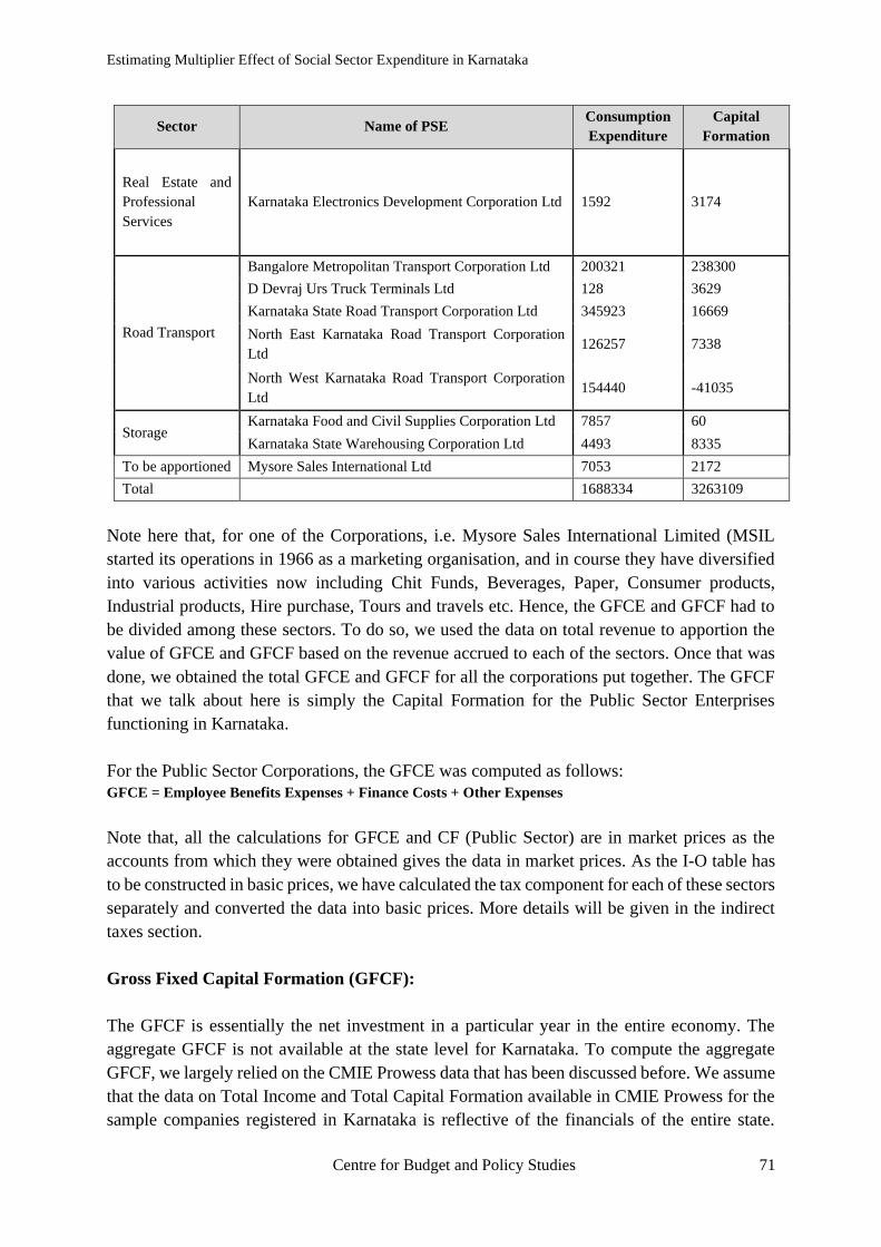
Estimating Multiplier Effect of Social Sector Expenditure in Karnataka
Centre for Budget and Policy Studies 71
Sector Name of PSE Consumption
Expenditure
Capital
Formation
Real Estate and
Professional
Services
Karnataka Electronics Development Corporation Ltd 1592 3174
Road Transport
Bangalore Metropolitan Transport Corporation Ltd 200321 238300
D Devraj Urs Truck Terminals Ltd 128 3629
Karnataka State Road Transport Corporation Ltd 345923 16669
North East Karnataka Road Transport Corporation
Ltd 126257 7338
North West Karnataka Road Transport Corporation
Ltd 154440 -41035
Storage Karnataka Food and Civil Supplies Corporation Ltd 7857 60
Karnataka State Warehousing Corporation Ltd 4493 8335
To be apportioned Mysore Sales International Ltd 7053 2172
Total 1688334 3263109
Note here that, for one of the Corporations, i.e. Mysore Sales International Limited (MSIL
started its operations in 1966 as a marketing organisation, and in course they have diversified
into various activities now including Chit Funds, Beverages, Paper, Consumer products,
Industrial products, Hire purchase, Tours and travels etc. Hence, the GFCE and GFCF had to
be divided among these sectors. To do so, we used the data on total revenue to apportion the
value of GFCE and GFCF based on the revenue accrued to each of the sectors. Once that was
done, we obtained the total GFCE and GFCF for all the corporations put together. The GFCF
that we talk about here is simply the Capital Formation for the Public Sector Enterprises
functioning in Karnataka.
For the Public Sector Corporations, the GFCE was computed as follows:
GFCE = Employee Benefits Expenses + Finance Costs + Other Expenses
Note that, all the calculations for GFCE and CF (Public Sector) are in market prices as the
accounts from which they were obtained gives the data in market prices. As the I-O table has
to be constructed in basic prices, we have calculated the tax component for each of these sectors
separately and converted the data into basic prices. More details will be given in the indirect
taxes section.
Gross Fixed Capital Formation (GFCF):
The GFCF is essentially the net investment in a particular year in the entire economy. The
aggregate GFCF is not available at the state level for Karnataka. To compute the aggregate
GFCF, we largely relied on the CMIE Prowess data that has been discussed before. We assume
that the data on Total Income and Total Capital Formation available in CMIE Prowess for the
sample companies registered in Karnataka is reflective of the financials of the entire state.
Estimating Multiplier Effect of Social Sector Expenditure in Karnataka
Centre for Budget and Policy Studies 72
Although this may seem like a limiting assumption, this was the best we could access for
anything at the state level. We computed the C/Y ratio for each of the sectors for which data
was available in CMIE (Figure A3.6). This ratio was multiplied with the Gross Value of Output
for Karnataka to arrive at GFCF for in Karnataka. For those sectors whose C/Y ratio was not
available from Prowess or the numbers were not reliable as it is difficult to disaggregate the
data for Karnataka, like say Air Transport as it is a large sector and the capital formation for
this sector cannot be assumed to solely represent the capital formation in Karnataka, we used
India C/Y ratio available from National Accounts Statistics (NAS) 2013-14 to compute GFCF
for these respective sectors. These four sectors included Forestry, Fisheries, Water and Air
Transport. This data from NAS included the GVO of Private Sector Corporations in India and
the GFCF for Private Sector Corporations.
GFCF for the Crops sector: The crops sector is largely unorganised and we have used NSS
70th Round Data on All India Debt and Investment Survey conducted between January -
December 2013. This provides us with the data on expenditure incurred in Farm Business that
include Capital Expenditure on Land, Livestock and Implements. The data presented includes
new purchases, major repairs and improvements made on these resources. To further capture
the private corporate sector in Agriculture, we followed the method prescribed by Narayana,
Vani and Kusuma (2011), who provide us the time series data for the period 1999-2000 to
2008-2009. This time series was extrapolated till 2014 by computing Compounded Annual
Growth Rate (CAGR). The share of the Corporate Sector GFCF in Agriculture forms three per
cent of the total Private sector GFCF in Agriculture and the remaining share is contributed by
Household (Unorganised) sector in Agriculture. This was added to the calculations of GFCF
which we did for the public sector using sources that included General Government Budget,
Local Budgets / Local Accounts and Public Sector Corporations, and followed a methodology
similar to the computation of GFCE to identify capital formation. Both these were added to
obtain the GFCF for the Crops sector.
GFCF for the Livestock and Public Administration sector: There was no data in CMIE for
the Livestock sector and Public Administration is a public service. Hence, for these two sectors,
we computed the Capital Formation by taking data from public accounts as described in the
GFCE computation and hence arrived at the GFCF data for these two sectors.

Estimating Multiplier Effect of Social Sector Expenditure in Karnataka
Centre for Budget and Policy Studies 73
Figure A3.6: Capital to Output (C/Y) Ratio used for computation of GFCF across sectors
Source: CMIE Prowess and National Account Statistics
A note on the estimation of Capital Formation in the Public Sector:
For the purpose of our study and analyses, we have also computed the capital formation in the
public sector by largely following the same method which we followed in the computation of
GFCE. Hence, the sources explored include General Government Budget, Local Budgets /
Local Accounts and Public Sector Corporations where each item was classified based on the
description into CE and CF. The difference between Additions in the Gross Block and
Deductions/Disposals in the Gross Block is taken as New Capital Formation in that year.
By deducting the public sector GFCF obtained using the above methodology from the total
GFCF gives us the data on the GFCF for the private sector.
Exports and Imports:
Data on exports and imports at state level is captured by Directorate General of Commercial
Intelligence and Statistics in quantity terms only. This is limited to data by sea route, air route,
river and railway route. However, no data on movement of goods by land is maintained by
them or in any other source. The data by sea route alone captures the value of transactions. For
Karnataka, the Visvesvaraya Trade Promotion Centre (VTPC) under the aegis of Department
of Industries and Commerce, Government of Karnataka complies and publishes the export data
for 19 commodities using data obtained from Director General of Commercial Intelligence and
Statistics, Kolkata, Export Promotion Councils (EPCs), Commodities Boards and other State
agencies. Trade & industry bodies also support the creation of this database. Assuming that
these 19 commodities make up most of the exports in Karnataka, we use this data to classify
the commodities across the sectors and hence the value of exports is obtained. However, no
15%
4%
-5%
11%
83%
26%
1%
51%
20% 18%
2% 0%
12% 14%9%
6% 7%
16%
4%
-10%
0%
10%
20%
30%
40%
50%
60%
70%
80%
90%
Estimating Multiplier Effect of Social Sector Expenditure in Karnataka
Centre for Budget and Policy Studies 74
such computation is available for imports and hence, as we already know the total value added
for the state from the SDP report, we assume the residual as the total value of imports for
Karnataka. The imports were then divided across the sectors based on the proportions in the I-
O table constructed by NCAER in 2013-14. The computations as discussed above help us
obtain the final demand components of the I-O table.

Estimating Multiplier Effect of Social Sector Expenditure in Karnataka
Centre for Budget and Policy Studies 75
Annexure 4: Net Indirect Taxes
The calculation of Net Indirect Taxes becomes important for the Input – Output table as the
role of the State affects the circular flow of income through leakages that takes place because
of taxes and subsidies. To arrive at Net Indirect Taxes, the detailed methodology is discussed
below.
The Total Indirect Taxes can be expressed as follows:
Total Indirect Taxes = Taxes on Intermediate Goods (Intermediate Consumption) + Taxes on Purchases
(by Households) + Taxes on Investment Goods (Capital Account of GFCF) + Taxes on Exports.
Taxes on purchases by Households:
Our starting point is the Household sector as we have the most disaggregated data on the
purchases (consumption expenditure) by this sector. For the purpose of our SAM we had
classified the household sector into 10 different occupational groups. Once this was classified,
we obtained the list of 448 items for which the private final consumption expenditure was
computed. For computing PFCE, we had computed by annualising the PFCE across each of
the 23 sectors and separately across each of the household groups. Please note that, the
consumption expenditure included the taxes paid by the consumer. As we have the list of 448
items and the respective item expenditures spent by each of those household groups, we
obtained the tax rates for each of the 448 items that the consumer would have paid by referring
at the VAT Rates for Karnataka in 2013-14 for goods, and the service taxes charged by the
Government of India for Services. There were also other taxes like the luxury tax,
entertainment tax etc, charged by the respective states. Some of them were also exempted from
tax (like many agricultural goods) and some items were levied excise duty by the state (liquor
items). One may argue that there is more number of items than just 448 but as our data on
consumption expenditure was limited to these 448 items, we assume it covers most of the
essential household expenditure. These 448 items have been divided into different baskets
depending on the item type, say, for example, food items, durable items, education spend etc.
While most of the spending happens for a particular item, each of the item groups has one
category which captures all the ‘other goods/services’ not mentioned in the item list (448) but
is still being incurred by the household. Hence, technically, the household expenditures have
been captured for more than just 448 items. Obviously, when this is the case, we will not have
a tax rate for these ‘other goods/services’ since we do not have information on the item for
which that expenditure was incurred. For these cases, what we did was to find the average tax
paid (by weighting). So, for example, for the group of items which included torch, lock,
umbrella, raincoat, lighter (bidi/ cigarette/ gas stove) and other minor durable-type goods, each
of these items have a different tax rate. Hence, for the item category ‘other minor durable-type
goods’ we used the weighted tax rate of the taxes paid on torch, lock, umbrella, raincoat, lighter.
For some of the services mentioned in the list of items, for example, laundry, cleaner, barber,
hair dresser etc., we are aware that some of these services provided by the formal sector are
chargeable. But applying the tax to all the household groups, especially rural and other urban

Estimating Multiplier Effect of Social Sector Expenditure in Karnataka
Centre for Budget and Policy Studies 76
household groups apart from the urban salaried class would give us an overestimated number
as we want to believe that these sectors avail services of the informal sector not coming under
the purview of tax. Hence, in such cases, we went with the assumption that only the ‘Urban
Regular wage / salary earning’ went for formal services and paid taxes, and hence, we
computed the approximate tax paid for these kinds of services for only such household groups.
The formula used for computing the taxes are as follows: Consumption Expenditure Value / (1+Tax Rate)
= Value of item before tax
Hence, Total Taxes Paid = Consumption Expenditure Value - Value of item before tax
Adding up the total taxes paid for each item across households, gives us the value of the total
taxes for each of the sectors when the items are grouped into the sectors.
Taxes on Intermediate Goods:
We described earlier the methodology of computing the indirect taxes for households. Based
on the expenditures incurred by households across various items, item groups which can be
grouped into the 23 sectors, we obtained the average tax rate for each of the household groups
and likewise, the overall tax rate for each sector. The table A4.1 below shows in detail these
tax rates.
Table A4. 1: Tax rates across sectors
Sector Grand Total
Agriculture 1.0%
Air Transport 5.0%
Communication 12.0%
Education 0.4%
Electricity, gas & Water Supply 0.6%
Forestry 0.0%
Health 2.8%
Hotels & Restaurants 2.7%
Livestock 0.6%
Manufacturing 8.6%
Mining 1.0%
Other Services 7.0%
Railway Transport 0.0%
Real Estate & Professional Services 0.0%
Road Transport 9.8%
Services incidental to transport 5.0%
Trade & Repair Services 11.5%
Water Transport 0.0%
Grand Total 3.9%
Source: Authors’ calculations
Estimating Multiplier Effect of Social Sector Expenditure in Karnataka
Centre for Budget and Policy Studies 77
So, 1% is the total taxes paid to the agriculture sector by the households. From the I-O table,
we have the data of the total intermediate consumption from each of the sectors. To that data,
we compute the value of taxes on these intermediate goods by assuming the average tax rates
as listed above to get the total taxes on the consumption of intermediate goods.
Taxes on purchases by Government:
There is no direct way of getting data on taxes paid by the government for its purchases. Hence,
we followed a similar methodology as mention above for computation of taxes on intermediate
goods. We used the weighted average tax rate for each of the sectors from the PFCE calculation,
applied those rates on the sector wise government purchases to obtain the taxes on purchases
by Government.
The overall data for indirect taxes at a state level is computed by multiple sources including
the data accrued from the Department of Commercial Taxes and Karnataka Annual Financial
Statement released by the Budget Finance Department. However, data is not available for each
of the 23 sectors of the I-O Table and SAM or the break up is not available as individual
components mentioned above. Hence, we used this data to verify the total taxes that we
obtained by addition of individual components. Our estimation of indirect taxes was
approximately 28% higher than what was for Karnataka from the above-mentioned sources.
We assume that, as both the methods uses a different method to estimate the total indirect taxes
collection, there is a chance for the data to not be equivalent.
The IOTT and SAM take into account the net indirect taxes, and hence, it becomes important
to look at the data on subsidies. We obtained the data on subsidies from the Overview of
Budget, Finance Department, 2015 document which gives us data on the subsidies provided by
the government across different items. These items were then classified to their sectors of origin
and the subsidies were computed sector-wise accordingly (Table A4.2) Once this data on
subsidies was obtained, we apportioned it according to the proportion of indirect taxes in each
of the categories including taxes on intermediate consumption, taxes on purchases by
households, taxes on purchases by government, taxes on capital goods and accordingly, sector
wise net indirect taxes were computed.

Estimating Multiplier Effect of Social Sector Expenditure in Karnataka
Centre for Budget and Policy Studies 78
Table A4.2: Subsidies in Karnataka
Type of Subsidy Sector In Rs. lakhs
Food Agriculture 304604
Transport Road Transport 69110
Power Electricity, Gas & Water Supply 546000
Industries Manufacturing 9884
Housing Construction 44804
Cooperation Financial Services 270480
Agriculture Agriculture 26278
Milk Livestock 68122
Others and Labour Apportion according to other sectors 71040
Agriculture & Horticulture Agriculture 47126
Animal Husbandry and Fisheries Livestock 1200
Milk Livestock 9576
Co-operation Financial Services 14750
Women & Child Development Other remaining services 37158
Housing Construction 71346
Education Education 25418
Commerce & Industries Manufacturing 16008
Source: Overview of Budget, Finance Department, 2015
Once all the components for the I-O table are computed, we then move on to compute the
components of the Social Accounting Matrix.

Estimating Multiplier Effect of Social Sector Expenditure in Karnataka
Centre for Budget and Policy Studies 79
Annexure 5: Construction of Components of Social Accounting Matrix
In the sections below, we will discuss the computation of each of these components which will
finally help us arrive at the Social Accounting Matrices.
Production Accounts
The production accounts are nothing but the Input-Output table which talks about the inter-
linkages between the different sectors. The method for its computation has been discussed
above.
Factors
The factors include the wage and non-wage component of the GVA and the net factor income
from ROW in the row totals and the total factor endowments in the columns include the
endowment of households, operating profits of private corporations, operating surplus for the
public sector corporations, the income from entrepreneurship earned by the Governments and
the depreciation on the capital account. Each of these have been computed as given below:
Wage and non-wage component
Within SAM, GVA is divided into wage and non-wage income. Different methods and sources
have been used to capture the wage and non-wage component of the GVA of each sector. The
method followed is given in brief below.
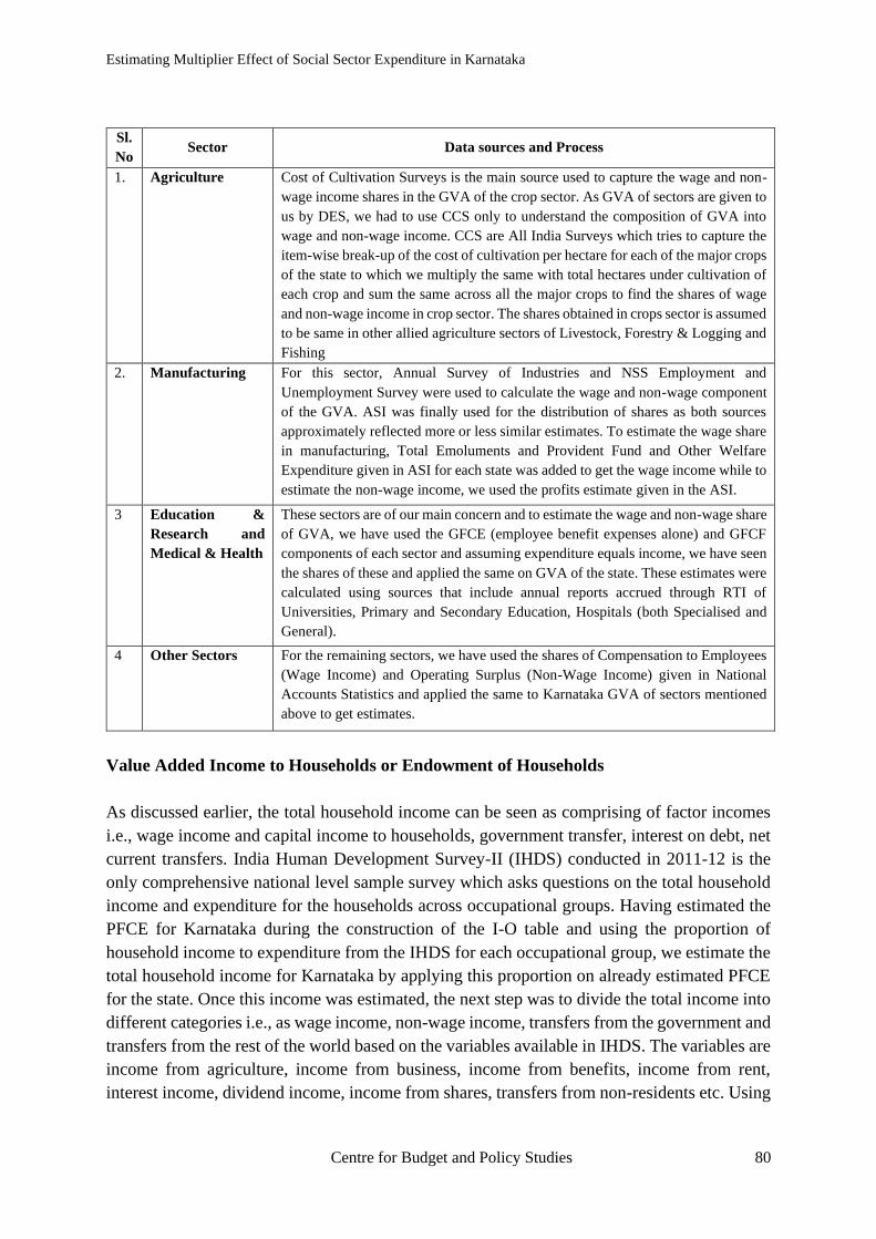
Estimating Multiplier Effect of Social Sector Expenditure in Karnataka
Centre for Budget and Policy Studies 80
Sl.
No Sector Data sources and Process
1. Agriculture Cost of Cultivation Surveys is the main source used to capture the wage and non-
wage income shares in the GVA of the crop sector. As GVA of sectors are given to
us by DES, we had to use CCS only to understand the composition of GVA into
wage and non-wage income. CCS are All India Surveys which tries to capture the
item-wise break-up of the cost of cultivation per hectare for each of the major crops
of the state to which we multiply the same with total hectares under cultivation of
each crop and sum the same across all the major crops to find the shares of wage
and non-wage income in crop sector. The shares obtained in crops sector is assumed
to be same in other allied agriculture sectors of Livestock, Forestry & Logging and
Fishing
2. Manufacturing For this sector, Annual Survey of Industries and NSS Employment and
Unemployment Survey were used to calculate the wage and non-wage component
of the GVA. ASI was finally used for the distribution of shares as both sources
approximately reflected more or less similar estimates. To estimate the wage share
in manufacturing, Total Emoluments and Provident Fund and Other Welfare
Expenditure given in ASI for each state was added to get the wage income while to
estimate the non-wage income, we used the profits estimate given in the ASI.
3 Education &
Research and
Medical & Health
These sectors are of our main concern and to estimate the wage and non-wage share
of GVA, we have used the GFCE (employee benefit expenses alone) and GFCF
components of each sector and assuming expenditure equals income, we have seen
the shares of these and applied the same on GVA of the state. These estimates were
calculated using sources that include annual reports accrued through RTI of
Universities, Primary and Secondary Education, Hospitals (both Specialised and
General).
4 Other Sectors For the remaining sectors, we have used the shares of Compensation to Employees
(Wage Income) and Operating Surplus (Non-Wage Income) given in National
Accounts Statistics and applied the same to Karnataka GVA of sectors mentioned
above to get estimates.
Value Added Income to Households or Endowment of Households
As discussed earlier, the total household income can be seen as comprising of factor incomes
i.e., wage income and capital income to households, government transfer, interest on debt, net
current transfers. India Human Development Survey-II (IHDS) conducted in 2011-12 is the
only comprehensive national level sample survey which asks questions on the total household
income and expenditure for the households across occupational groups. Having estimated the
PFCE for Karnataka during the construction of the I-O table and using the proportion of
household income to expenditure from the IHDS for each occupational group, we estimate the
total household income for Karnataka by applying this proportion on already estimated PFCE
for the state. Once this income was estimated, the next step was to divide the total income into
different categories i.e., as wage income, non-wage income, transfers from the government and
transfers from the rest of the world based on the variables available in IHDS. The variables are
income from agriculture, income from business, income from benefits, income from rent,
interest income, dividend income, income from shares, transfers from non-residents etc. Using

Estimating Multiplier Effect of Social Sector Expenditure in Karnataka
Centre for Budget and Policy Studies 81
these variables, we calculated the proportions of these components in the total income and used
that to estimate the endowment of households.
Operating Profits of Private Corporate Sector
There is no data source which gives us the operating profits of the private corporate sector at
the State level. CMIE is the only source that can give us some data on companies. We took a
ratio of the operating profits of companies registered in Karnataka to India separately for
financial companies and non-financial companies which accounted for about 3.5% and 8.4%
respectively. By applying the above proportions which we obtained for financial companies
and non-financial companies on the operating surplus of the financial and non-financial
companies in India on NAS data for India, we estimated the operating profits for Karnataka.
Operating Surplus
This was estimated as the summation of net rent, net interest, net profit income obtained from
the annual reports procured from Public Sector Undertakings.
Income from Entrepreneurship
It is the income received by the government from the factors i.e. labour and capital for the
services that is rendered by them. These comprises of profits, income from property, net interest
received from various authorities, from other sectors, and other kinds of property receipts. This
number is computed and given by the Economic – cum – Purpose Classification Report 2011-
12 to 2018-19 taken from the Statement on Income and Outlay Account of Administrative
Departments (Receipts).
Depreciation on Capital Account
This component was directly obtained from the SDP Report 2015-16 that provided us CFC
data for each of the 23 sectors for the year 2013-14. This was used as is for the construction of
SAM for Karnataka.
Net Factor Income
Net Factor Income constitutes remittances received and sent by the factors. To estimate this
component, we have used RBI Bulletin that gives us the share of Karnataka in the total
remittances received to be 15 percent. This has been assumed as Karnataka’s share in the credit
and debit reflected in Balance of Payments Statement and further is used to estimate the labour
and capital income. For the labour income, we have taken the net of the data on Compensation
of employees and for the capital income, we have taken the net of the data on Investment
income.
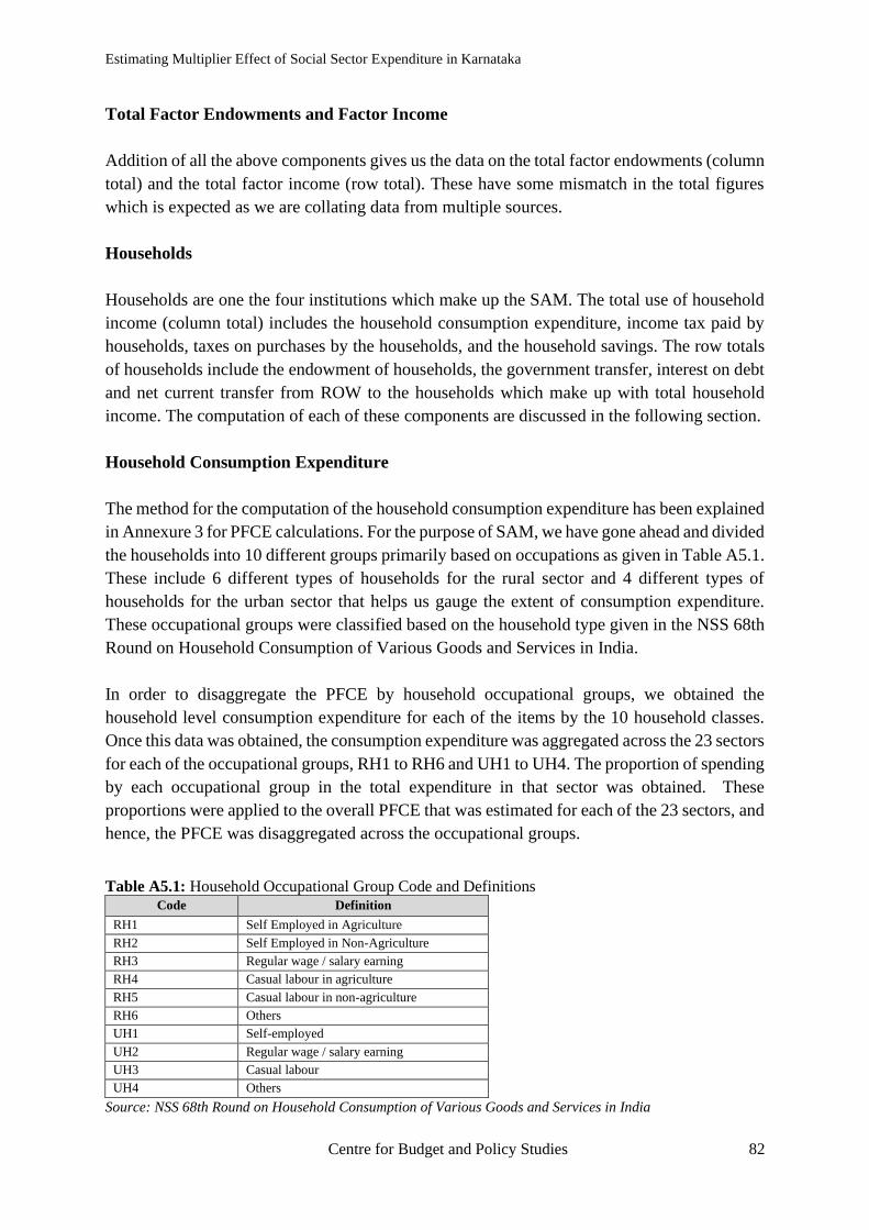
Estimating Multiplier Effect of Social Sector Expenditure in Karnataka
Centre for Budget and Policy Studies 82
Total Factor Endowments and Factor Income
Addition of all the above components gives us the data on the total factor endowments (column
total) and the total factor income (row total). These have some mismatch in the total figures
which is expected as we are collating data from multiple sources.
Households
Households are one the four institutions which make up the SAM. The total use of household
income (column total) includes the household consumption expenditure, income tax paid by
households, taxes on purchases by the households, and the household savings. The row totals
of households include the endowment of households, the government transfer, interest on debt
and net current transfer from ROW to the households which make up with total household
income. The computation of each of these components are discussed in the following section.
Household Consumption Expenditure
The method for the computation of the household consumption expenditure has been explained
in Annexure 3 for PFCE calculations. For the purpose of SAM, we have gone ahead and divided
the households into 10 different groups primarily based on occupations as given in Table A5.1.
These include 6 different types of households for the rural sector and 4 different types of
households for the urban sector that helps us gauge the extent of consumption expenditure.
These occupational groups were classified based on the household type given in the NSS 68th
Round on Household Consumption of Various Goods and Services in India.
In order to disaggregate the PFCE by household occupational groups, we obtained the
household level consumption expenditure for each of the items by the 10 household classes.
Once this data was obtained, the consumption expenditure was aggregated across the 23 sectors
for each of the occupational groups, RH1 to RH6 and UH1 to UH4. The proportion of spending
by each occupational group in the total expenditure in that sector was obtained. These
proportions were applied to the overall PFCE that was estimated for each of the 23 sectors, and
hence, the PFCE was disaggregated across the occupational groups.
Table A5.1: Household Occupational Group Code and Definitions Code Definition
RH1 Self Employed in Agriculture
RH2 Self Employed in Non-Agriculture
RH3 Regular wage / salary earning
RH4 Casual labour in agriculture
RH5 Casual labour in non-agriculture
RH6 Others
UH1 Self-employed
UH2 Regular wage / salary earning
UH3 Casual labour
UH4 Others
Source: NSS 68th Round on Household Consumption of Various Goods and Services in India

Estimating Multiplier Effect of Social Sector Expenditure in Karnataka
Centre for Budget and Policy Studies 83
Household Income
The household income has been estimated using mainly the sample data from the India Human
Development Survey (IHDS 2011-12). We classified the household groups in the IHDS to
match the household occupational classifications in the National Sample Survey data. Once
this was done, we obtained the total income and expenditure data from the IHDS for the sample
from Karnataka and thus obtained the ratio of income to expenditure. These ratios were they
applied on the consumption expenditure data estimated during the PFCE calculation to obtain
the household income data for each of the 10 occupational groups.
Income Tax from Households
Income tax from households also forms a component of the total government earnings.
Personal income tax in India is collected by the Central Government and passed on to the State
Governments. The Central Board of Direct Taxes gives us data on the direct tax collection
across the states. This is provided in the Time Series Data Financial Year 2000-01 to 2018-19
by Income Tax Department. The data provided at the state level is limited to total direct tax
collected from all states with no breakup of its components. To arrive at the share of each
component at the state level, we assumed the India’s proportion of personal income tax (38%),
corporate income tax (62%) and applied this on Karnataka’s total direct taxes. In order to divide
the total personal income tax across the household occupational groups, we assumed the
proportions of household incomes to be the proportion of taxes collected
Household Savings
The total use of household income can be expressed as:
Total use of household income = Household Consumption + Income Tax from Households + Taxes on
purchases by Households + Household savings.
The data on household savings at the state level is unavailable and there is no way of estimating
this component. Therefore, as we had already computed the household expenditure, the income
tax from households and the taxes on purchases by households, we are using the residual
method to estimate the household savings
Govt. Transfer, Interest on Debt
This component is part of total Household Income which is received by households as transfers
(no quid pro quo) and interest income paid by government for the bonds held by households.
These form part of disposable income of the households. This is calculated using IHDS data
where the total household income procured is divided into wage income, capital income,
transfer from domestic sources and transfer income from ROW and other sources. These
proportions obtained across the ten household groups were then applied on the total household

Estimating Multiplier Effect of Social Sector Expenditure in Karnataka
Centre for Budget and Policy Studies 84
income to obtain the government transfers. The data to get the interest on debt at a household
level is very limited and hence this value could not be computed.
Net Current Transfer
Current transfers are those benefits, either in the form of cash or kind, made or received by
households, to or from non-resident households independent of the source of income of the
sender and the relationship between households. Current transfers directly affect the level of
disposable income and influence consumption of goods of services. This component is
estimated using the proportions that we obtained by bifurcating the total household income
from IHDS into various components across all types of occupational categories. This was
multiplied with the proportion of current transfers estimated for Karnataka from RBI bulletin
assuming the share of KA in total current transfers to be 15 percent.
Private Corporations
The total private corporate income (column total) includes the corporate taxes and the corporate
savings and in the row totals it includes the operating profits and the interest on debt. The
calculations for each of these components has been discussed below.
Corporate Taxes
To estimate this component of the matrix, we relied on Central Board for Direct Taxes (CBDT)
which gives state-wise data on the total Direct taxes and its types including Corporate Income
Tax, Personal Income Tax and Other Direct Taxes. Corporate Taxes amount to 62 percent of
the total Direct tax collection in India. By applying this proportion on the total direct taxes
collected in the state as obtained from the CBDT, we estimated the corporate taxes in the state.
Income of the private corporate sector
The same procedure that was followed for the calculations of the operating profits for the
private corporate sector was followed for the computation of its income using CMIE for
Karnataka. We took a ratio of the total income of companies registered in Karnataka and India
separately for financial companies and non-financial companies which accounted for about 6%
and 5% respectively for the state. By applying the above proportions which we obtained for
financial companies and non-financial companies on the GVA of the financial and non-
financial companies in India using NAS, we estimated the Private Corporate Income for
Karnataka.
Interest on Debt
This component is part of the income of private corporate sector i.e., interest income received
by the corporate sector on the bonds and securities issued by the government. To estimate this

Estimating Multiplier Effect of Social Sector Expenditure in Karnataka
Centre for Budget and Policy Studies 85
component, we used the residual method by calculating the difference between the Income and
operating profits of private corporations.
Corporate Savings
This component was also computed through backward calculation by first estimating the
Private Corporate Income and Corporate Taxes and the difference between the two gave us the
Corporate Savings.
Government
The column totals for the government sector includes the government consumption,
government transfer, interest on debt, the interest on debt by the private corporations, the taxes
on purchases by the government and the government savings. The row totals include income
from entrepreneurship, income tax from households, corporate taxes, total indirect taxes and
net capital transfers and which form the total government earnings. The method to arrive at
each is discussed in the above sections.
Government Savings
To estimate Govt. savings, we calculated the difference between Total Expenditure of the State
Government reported in ECP (2011-12 to 2019-20) and Total Receipts (Both Administrative
Departments & Departmental Enterprises). It shows there is dissaving in the state due to excess
expenditure.
Net Capital Transfer
This is estimated using the data from RBI Balance of Payment Statement with the assumption
that Karnataka’s share to be 15 percent. Capital Transfers do not affect the level of disposable
and therefore accounted under ROW and Government.
Total Government Earnings
This was derived through summation of all the components in the respective row to arrive at
the earnings of government from different sources.
Capital Account
The column totals of the capital account include the gross fixed capital formation, and the taxes
on investment goods to arrive at the aggregate investment and the row totals includes the
components of the gross savings of the economy. The computation of most of the components
have been discussed in the previous sections. Given below is the computation of the foreign
savings.
Estimating Multiplier Effect of Social Sector Expenditure in Karnataka
Centre for Budget and Policy Studies 86
Foreign Savings
This was calculated using residual method. The savings of all other institutions was estimated
first and alongside, we were able to arrive at Gross Savings of the economy which is equal to
Aggregate Investment in the economy. The difference between Gross Savings (Aggregate
Investment) and savings of all other institutions helped us derive Foreign Savings of the state.
Rest of the World Accounts (ROW)
Foreign Exchange Payments
This was derived through summation method, and this is equivalent to the imports in the
economy.
Taxes on exports: This was taken as zero as the Karnataka state government did not tax exports
in the 2013-14 period.
Based on the methodology described above, we finish the construction of the Input-Output
table and Social Accounting Matrix for Karnataka for 2013-14.

Estimating Multiplier Effect of Social Sector Expenditure in Karnataka
Centre for Budget and Policy Studies 87
Annexure 6: Tools to estimate Multiplier
Supply side versus Demand side theories of Growth
A brief description of growth and respective theories in the discipline of economics would help
provide us with understanding and validation for the use of respective methods in our research.
The commotion around Growth or GDP (Gross Domestic Product) statistics in itself reflects
the significance of the variable. More importantly, growth signifies availability of goods and
services for the population to consume and also implies growth in incomes though contingent
on factors like nature of employment, political structure, and other legal, socio, economic
structures. National Income or GDP is the surplus of annual output of goods and services over
and above the needs of annual input replacement that can be used either for present
consumption or for investment. Growth implies transformation process in economic processes.
To induce the transformation, the discipline presents largely two broad theories, supply based
growth theories and demand-based growth theories.
Supply based growth theories as the name suggests is based on a belief that the free enterprise
economy is self-regulating with growth in the market economy consequently expected to have
a trickle-down effect and subsequently leading to increase in aggregate incomes. The theories
provide no scope for government intervention or made provision for a passive government role
in stimulating the economy because it assumes that in societies and economies, growth can be
path independent and therefore ahistorical. Supply based growth theories are based primarily
on Solow Growth Model and Endogenous Growth theories.
Demand based growth theories believe that growth process is path dependent and cumulative.
Past affects the present and the future and therefore history is imperative in the economy’s
growth process. They view the growth process as non-linear, and therefore historical. This
implies that demand-based growth theories call for active government intervention in
stimulating growth that could be far away from natural rate of growth. In these theories,
demand deficiency is a structural problem that can be corrected only with government
intervention through policies that increase aggregate demand. These theories depend on a frame
that understands economy as an integrated system and production as a social activity. Demand
based growth theories are based on the multiplier effects of autonomous demand components.
Conventional versus alternative approaches
The tools that can be employed to study the multiplier effect can be broadly categorised to be
based on two approaches: Neo-classical approach and Alternative (Heterodox) approach. A
brief account of the basic differences between these approached is discussed further.
Classical/Heterodox/Alternative approach is based on an economic theory where analysis of
all economic processes of production, distribution, exchange and accumulation is based on an
idea of surplus (quantity dynamics) and subsequently price system is decided based on
production conditions. Therefore, this frame provided the base to analyse growth or

Estimating Multiplier Effect of Social Sector Expenditure in Karnataka
Centre for Budget and Policy Studies 88
accumulation. On the other hand, Neo-classical approach originating in the late 19th century
with the works of Jevons, Walrus and Marshall changed the scope of economic analysis from
production to exchange (markets/circulation) and from accumulation to allocation as the base
idea was scarcity rather than surplus. The focus of neo-classical framework was on the problem
of choice and the idea of utility, given the resources; and it applied the marginalist principles
of supply and demand apparatus to economic questions.
There are various methods and tools to estimate multiplier and broadly these can be classified
as mentioned above into conventional approaches (neoclassical) and alternative approaches.
The tools under conventional (neoclassical) approaches include Vector Auto-Regressive
methods, Computable General Equilibrium method and Dynamic Stochastic General
Equilibrium Method. These tools under conventional Approaches believe in supply side
theories where investment is dependent variable. Alternative approaches on the other hand
include Input-Output Model (IOM) and Social Accounting Matrix (SAM) which believes in
integrated economic system and investment as an autonomous variable.
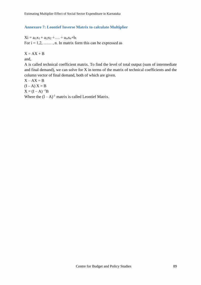
Estimating Multiplier Effect of Social Sector Expenditure in Karnataka
Centre for Budget and Policy Studies 89
Annexure 7: Leontief Inverse Matrix to calculate Multiplier
Xi = ai1x1 + ai2x2 +…. + ainxn+bi
For i = 1,2, …… , n. In matrix form this can be expressed as
X = AX + B
and,
A is called technical coefficient matrix. To find the level of total output (sum of intermediate
and final demand), we can solve for X in terms of the matrix of technical coefficients and the
column vector of final demand, both of which are given.
X – AX = B
(I – A) X = B
X = (I – A) -1B
Where the (I – A)-1 matrix is called Leontief Matrix.
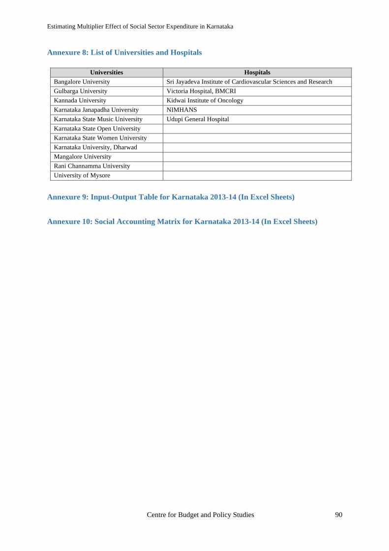
Estimating Multiplier Effect of Social Sector Expenditure in Karnataka
Centre for Budget and Policy Studies 90
Annexure 8: List of Universities and Hospitals
Universities Hospitals
Bangalore University Sri Jayadeva Institute of Cardiovascular Sciences and Research
Gulbarga University Victoria Hospital, BMCRI
Kannada University Kidwai Institute of Oncology
Karnataka Janapadha University NIMHANS
Karnataka State Music University Udupi General Hospital
Karnataka State Open University
Karnataka State Women University
Karnataka University, Dharwad
Mangalore University
Rani Channamma University
University of Mysore
Annexure 9: Input-Output Table for Karnataka 2013-14 (In Excel Sheets)
Annexure 10: Social Accounting Matrix for Karnataka 2013-14 (In Excel Sheets)
Estimating Multiplier Effect of Social Sector Expenditure in Karnataka
Centre for Budget and Policy Studies 91
Notes

Estimating Multiplier Effect of Social Sector Expenditure in Karnataka
Centre for Budget and Policy Studies 92
Notes

Estimating Multiplier Effect of Social Sector Expenditure in Karnataka
Centre for Budget and Policy Studies 93
Notes

Estimating Multiplier Effect of Social Sector Expenditure in Karnataka
Centre for Budget and Policy Studies 94
Notes
Related Documents


